1

CHAPTER 1�

INTRODUCTION

The Asian Arowana (Scleropages formosus) is an ornamental and primary

freshwater fishes that is strictly intolerant of saltwater. It’s commonly known as the

Dragonfish and belongs to the order Osteoglossiformes (Nelson, 1994).The Asian

arowana has obtained a special status in the world particularly in some Asian countries

such as Japan and China as a very popular but very expensive aquarium fish (Goh &

Chua, 1999). The name of Dragon fish comes from their resemblance to Chinese dragon

and known as lucky fish by many people (Hu et al., 2009).

This fish is listed as an endangered species in the 2006 IUCN Red List (Kottelat

et al., 1996) and also is classified as threatened a species with danger of extinction in the

CITES list since 1980 (Joseph et al., 1986), therefore farmers are required to attain

permission when culturing it (Dawes et al., 1999). According to the World Conservation

Union Red list 2007, it is estimated 2,491 freshwater fishes (43%) or 1,074 species fall

into the “threatened’’ class. Furthermore, this fish consists of geographically isolated

strains distributed at different locations around South East Asia that were probably

connected to freshwater habitats during the Pleistocene glacial ages (Stearn et al., 1979).

Generally, there are three main colour varieties for Asian arowana including Green,

Golden and Red along with distinct sub-varieties (Goh & Chua, 1999).

2

The keeping of ornamental fish is the most widespread animal related hobby in

the world that their attraction and value in the market depend on the diversity of species,

great variety of colour, shape, behaviour and origin (Tang, 2004). In Malaysia, the

ornamental fish trade is almost exclusively made up of freshwater fish species.

Morphological features have been commonly used to distinguish fish. The

features include the body shape, relative size of the body parts, size and count of the

scales, the relative position, number and type of fin rays, and the body color pattern

(Strauss & Bond, 1990). However, species identification solely based on the

morphological features can be misleading due to presence of intraspecific variation and

subtle differences observed in many closely related species (Teletchea, 2009).

Moreover, the identification at early developmental stage can be more difficult and

challenging for this fish since it constantly undergoes phenotypic changes in its

different life stages and develops its own distinct features at a later life stage. Thus,

DNA based identification method is seen to offer greater utility to screen and identify

the fish, as it can be performed on any developmental stage using any body part or

organic material from the fish (Teletchea, 2009).

Due to environmental destruction, Asian arowana is currently uncommon in the

Malaysia while they were widely distributed previously. In fisheries, the conservation of

genetic resources is a great task in long-term management because, there might be a

need of recovering the lost or decreased genetic variation and they might be possessing

special genes or important genetic information (Tang, 2004).�

3

The lack of molecular and genetic information about Asian arowana has

hindered the biological study of this fish. Mitochondrial DNA markers are expected to

be a useful tool for the understanding the fish’s molecular biology (Yue et al., 2006). To

date, Mitochondrial DNA sequences have shown some success in phylogenetics studies

of many organisms; due to its lack combination (Hayashi et al., 1985; Clayton, 1992);

mainly maternal inheritance nature (Kondo et al., 1990; Gyllestein et al., 1991);

compact gene packing, with little noncoding intergenic nucleotides and some nucleotide

overlapping between genes encoded in opposite strands (Cantatore et al., 1987);

Multicopy status in cell, and faster evolution rate which allows variation sufficient to

delineate closely related species compared to the nuclear genes (Brown et al., 1982;

Drake et al., 1998).

In this study, mitochondrial conserved markers such as Cytochrome c oxidase

subunit I (COI) and Cytochrome b (Cyt b) are used for molecular identification of Asian

arowana. DNA barcoding is one of the molecular identification tools which is based on

short, standardized genes that are able to provide accurate species identification (Hebert

et al., 2003). Cytochrome c oxidase I (COI) gene, under the Fish Barcode Initiative,

FISH-BOL has been used extensively for species identification and discovery of cryptic

species (Ward et al., 2005). DNA barcodes comprise approximately of 600-bp

sequences of mitochondrial DNA that have become eminent in the world of genetic

applications for global biodiversity assessment (Rubinoff et al., 2006). The efficiency

of DNA barcoding depends on the degree of sequence divergence among species and

species-level identification and is relatively straightforward when the average genetic

distance among individuals within a species does not exceed the average genetic

distance between sister species (Hubert et al., 2008). In addition, the mitochondrial

cytochrome c oxidase subunit I gene (COI) provide valuable information in species

4

identification to complete taxonomic information and validation of systemic position

and phylogeny (Machordom et al., 2003; Smith et al., 2004; Donald et al., 2005).

The most commonly used mtDNA marker is Cytochrome b (Cyt b) in

phylogenic studies (Briolay et al., 1998). This mtDNA marker is considered to be

variable enough to explain doubts on the population level, and conserve enough to

clarify deeper phylogenetics relationships. The wide application of cytochrome b has

made a status as universal metric, in the sense that studies can be easily compared

(Mayer, 1994).

Main objectives of this study are;

1. To be able to DNA barcode the different Arowana strains using Cytochrome c

oxidase subunit 1(COI)

2. To infer the phylogenetic analysis of arowana strains using Cytochrome b and

Cytochrome c oxidase I (COI)

The hypothesis:

� Different Arowana starins will have their unique DNA barcodes

� The Malaysian golden arowana and Indonesian golden arowana can be

differentiated by its cytochrome b genes

5

CHAPTER 2

LITERATURE REVIEW

2.1 Asian Arowana

2.1.1 Classification of Asian Arowana

Asian Arowana is a primitive fish from the Jurassic era (Bonde, 1979), belonging

to the order Osteoglossiformes and is one of the ancestral teleost clades with bony

tongue being one of their primitive features. The Osteoglossiformes order is composed

of two suborders, Osteoglossoidei and Notopteroidei. The Osteoglossoidei suborder

consists two families including Osteoglossidae and Pantodontidae. Osteloglossidae

family is further divided into two subfamilies, Osteoglossinae and Heterotidinae. The

family Pantodontidae has only one species, Pantodon buchholzi or butterfly fish

(Nelson, 1994).

The subfamily Osteoglossinae is divided into two genera, Osteoglossum and

Scleopages. There are two species of Osteoglossum in South America including

Osteoglossum bicirrhosum and Osteoglossum ferreirai which are referred to as the

silver arowana and black arowana respectively. There are three species in Scleopages

genus. Scleropages jardinii in the Gulf Saratoga or Nothern Spotted Barramundi and

Scleropages leichardti are found in Australia while Scleropages formosus, the Asian

arowana is distributed in the Southeast Asian regions (Dawes et.al., 1999). The

Subfamily Heterotidinae consists of Arapaima gigas found in South America and

Heterotis niloticus niloticus distributed in Niger and the upper Nile (Dawes et al.,

1999). In 1844, first time it was described by Muller and Schlegel for the genus

Osteoglossum and coined by Nelson in 1994 the present name Scleropages formosus

6

based on morphological data and supported by Kumazawa and Nishida in 2000 based

on the molecular phylogenetic data.

Kingdom Animalia

Phylum Chorodata

Class Actinopterygii

Subclass Neopterygii

Order Osteoglossiformes

Family Osteoglossidae

Genus Scleropages

Species formosus

Due to high demand and over exploitation of natural populations, the

Convention of International Trade in Endangered Species of Wild Fauna and Flora

(CITES) has classified arowana as a highly endangered species under its Appendix I list

(Joseph et al., 1986). In addition, several reproductive characteristics such as low

fecundity, oral brooding habit and open-water spawning makes this species vulnerable

to overexploitation (Tang, 2004).This kind of fish is now bred regularly in Singapore

and sold with CITES’ permission.

7

2.1.2 Distribution of Asian Arowana

The Asian arowana (Scleropages formosus) is commonly known as the

Dragonfish, Asia Bonytongue, kelisa or baju rantai (Tang et al., 2004) widely

distributed in Peninsular Malaysia, Sumatra, Thailand, Cambodia and Kalimantan

(Tang et al., 2004). In Malaysia, this fish can be found in certain rivers which are

located in northern and southern regions such as Penang, Johor, Pahang and Terengganu

(Tang, 2004). This fish can also be found in some lake in northern regions such as

Kenyir Lake, Bukit Merah Lake (Suleiman, 1999).

2.1.3 Habitat of Arowana

In nature, the arowana can be found in herbaceous swamps or marshland, lakes,

rivers and mining pools. This fish prefers to live in still or slow-flowing waters which

are turbid or weedy (Dawes et al., 1999).

2.1.4 Morphology

This arowana exhibites a knife shaped compressed body while the abdomen is

keeled. The gap of the mouth is very large and the lower jaw sticks out. The dorsal fin

base is shorter than the anal fin base and the anal fin base is longer than the head length

(Suleiman, 1999). This fish is able to grow up to around 90 cm .The distinction of

arowana sexes is not easy when they are young. In general, males are longer than

females in size and look slimmer while females have more rounded bodies (Dawes et

al., 1999).

8

2.1.5 Strain of Asian Arowana

There are four commercial verities of Asian arowana (Pouyaud et al., 2003)

including Malaysian Gold Arowana, Green Arowana, Indonesian Gold Arowana,

Indonesian Red Arowana (Pouyaud et al., 2003)

2.1.5.1 Golden Arowana

Golden Arowana or Blue Base Gold arowana is the most popular and can fetch

high price in the market (Tang, 2004). Malaysian Golden arowana is native to Bukit

Merah Lake, Perak (Suleiman, 1999). The scales may have different colors such as

gold; silver or blue (Figure 2.1).

2.1.5.2 Green arowana

This variety of Arowana is the most common and is widespread throughout

Southeast Asia which is found in Malaysia, Thailand, Vietnam and Myanmar (Kottelat

et al., 1993). In Malaysia this variety is distributed in Terengganu, Pahang and Johor

(Ng & Tan, 1999; Suleiman, 1999). This fish has olive scales and a prominent lateral

line. Young fish has yellow fins while the fins of the adult are dark green in color

(Figure A1).

2.1.5.3 Indonesian Gold Arowana

Indonesian Gold arowana is found in Sumatra island of Indonesia (Dawes et al.,

1999). The scales are copper-gold in color. Scales above the lateral line, dorsal fin and

9

upper half of its tail are dark green (Figure A2).The lower half of its tail fin, dorsal fin

and anal fin have purplish-red to brownish-red color (Dawes et al., 1999).

2.1.5.4 Indonesian Red Arowana

Indonesian Red arowana is the most well known variety which is found in

Indonesia’s Kalimantan province (Dawes et al., 1999). This variety (Figure A3) can be

divided into the first red class and the second red class and it is difficult to differentiate

the first class from the second class when the fish is young (Tang, 2004).

In addition, Goh and Chua (1999) reported that there are four naturally occurring

varieties found in different geographical locations: Cross back golden or Blue Malayan

Bonytongue (native to Bukit Merah and Pahang, Peninsular Malaysia), Super red

(native to West Kalimantan, Indonesia), Green (native to Peninsular Malaysia,

Indonesia, Myammar, Thailand) and Red-tail Gold (Figure A4) (native to Pekan Baru

and Jambi, Indonesia).In this study, Silver Arowana (Osteoglossum bicirrhosum) was

also used as a single species which is the one of the most popular ornamental fish in

South America (Figure A5).

Figure 2.1 Golden Arowana, taken from: Breeding Malaysian, Scleropages formosus in Concrete Tanks (Mohamad Zaini Suleiman, 2003)

10

2.2 Mitochondrion DNA (mtDNA)

Animal mtDNA is small and circular which has been widely used as one of the

many molecular tools and is extremely useful for species identification of major

vertebrate phyla (Murray et al., 1995; Branicki et al., 2003; Ward et al., 2005).

Mitochondrion is responsible for transferring energy from food to a form that cells are

able to use. However, most DNA is packaged in the nucleus, while mitochondria also

have a small amount of its own DNA. Mitochondrial DNA can be also defined as a

single type of circular double-stranded DNA including the light (L) strand and heavy

(H) strand. Light strand is rich in cytosine while heavy (H) strand is rich in guanines

making approximately 16 kbp length of mitochondrial genome a GC rich region (Brown

et al., 2005).

During zygote formation, a sperm cell contributes its nuclear genome to the egg

cell but not for its mitochondrial genome. Therefore, mitochondrial genome is known as

maternally inherited and both males and females receive their mitochondrial DNA from

their mother (Strachan & Read, 1999). Because of this, mitochondria are rather

reasonable markers to be used in detecting the correlation of the fish using maternal

inheritance.

Most of animal mitochondrial DNA contains 37 genes (Boore, 1999) that are all

essential for normal mitochondrial function. Among these genes, 13 genes provide

instructions for making enzymes contributed in oxidative phosphorylation process. The

rest of genes provide instructions for making molecules called transfer RNA (tRNA)

and ribosomal RNA (rRNA), which are chemical cousins of DNA. These types of RNA

help assemble protein building blocks (amino acids) in functioning proteins (Boore,

11

1999).The initial sites for mtDNA replication and mtRNA transcription are located at

one non-coding control region called D-loop (Boore, 1999). Mitochondrial DNA

possesses several advantages over nuclear DNA. According to Drake’s observation,

threat of DNA mutation is inversely related to the size of the genome. Hence, nuclear

DNA undergoes relatively slow mutation compared with mtDNA and, for this reason,

would require a much longer nucleotide sequence which is necessary with mtDNA in

order to provide a barcode capable of differentiating species. Each mitochondrion

contains several complete sets of mitochondrial genes and, therefore, when sample

tissue is limited, the mitochondrion offers a relatively abundant source of DNA (Drake,

et al., 1998).

Figure 2.2 Schematic representation of the circular molecule of the “conserved” vertebrate mitochondrial genome. Genes outside and inside the circle are transcribed in the H and L strands, respectively. Protein-coding genes are represented as follows: Cyt b - cytochrome b; CO I, CO II and CO III - subunits I, II and III of the cytochrome oxidase; ND1-6 - subunits 1 to 6 of the NADH reductase. tRNA are represented by their three-letter amino acid abbreviations. Picture taken from review article (Sérgio Luiz Pereira, Genetics and Molecular Biology, 23, 4, 745-752, 2000).

12

2.3 Mitochondrion DNA markers

Molecular genetic markers have become a well-established and valuable tool for

many applications in population genetics, conservation biology and evolutionary studies

as well as for mapping projects (Jarne & Lagoda, 1996). Vertebrate mitochondrial DNA

comprises of 6 different markers including, protein coding regions such as cytochrome

b, cytochrome c oxidase subunits (COI, II, III), ND1-6 (subunits 1- 6 of the NADH

reductase), non protein coding regions involving D-loop control region, 12s rDNA and

16s rDNA (Sérgio, 2000). Among these markers, cytochrome b, cytochrome c oxidase

subunits I, II, III and ND1-6 are considered as conserved markers (Figure 2.2). These

markers have their own application in different studies (Sérgio, 2000), For example D-

loop control region is frequently used in population studies due to the high variability in

its nucleotide sequence (Brown et al., 1996; Gissi et al., 1998; Ursing & Arnason,

1998), while protein-coding genes such as cytochrome b are generally used for

phylogenetic relationship studies at various levels within population (Sérgio, 2000).

2.3.1 Cytochrome c oxidase subunit I (COI)

Cytochrome c oxidase subunit 1 gene known as single short sequence of

mtDNA which is able to code a large transmembrane protein found in the

mitochondrion which is highly conserved among species. Cytochrome c oxidase protein

works as the terminal electron acceptor in the respiratory chain for reduction of oxygen

to water (Waugh, 2007). A segment near the 5-terminus of COI has been selected as a

barcode region for some of the animal groups (Hebert et al., 2003).

13

Hebert and co-workers have achieved the successes of DNA barcoding in a

series of publications. What is new and debatable is the idea of using just a small

portion of a single gene to identify species from a wide taxonomic range, including

animals such as birds, fish and insects (Hebert et al., 2004; Ward et al., 2005;

Hajibabaei et al., 2006). In order to obtain DNA barcodes from all species on the

planet, DNA barcoding has formed one site as Consortium for the Barcode of Life.

Therefore, developments in sequencing technology mean that sequences can be

obtained rapidly and inexpensively, so that this barcoding technique may seem

conceivable and worthwhile.

Some individuals of North American birds have been identified at species level

based on COI that has had a success with rate ranging from 98 to 100% (Hebert et al.,

2004). Two studies convincingly indicate the efficacy of DNA barcoding to recover

biologically important species. First of all, within a single morphologically identified

skipper butterfly species, DNA barcoding separated 10 cryptic species (Hebert et al.,

2004). Second, morphologically indistinguishable parasitoid flies (Tachinidae) were

shown to be comprised of groups of separate host-specific cryptic species (Smith et al.,

2006). Recently, DNA barcoding has discriminated the freshwater fish species from the

well-known Canadian fauna, nearly 200 fish were considered as species with high

economic value like salmons and sturgeons (Hubert et al., 2008).

In general, fishes constitute a highly diverse group of vertebrates that exhibit

deep phenotypic changes during development. Freshwater fishes show more population

differentiation than marine species even though marine species can show significant

differentiation (Ward et al., 1994).

14

In case of phylogenetic relationships based on COI, 28 Indian carangid fish

species were identified (Persis et al., 2008). Sequence analysis of COI gene very clearly

indicated that all the 28 fish species fell into five distinct groups, which are genetically

distant from each other and exhibited identical phylogenetic reservation. All the COI

gene sequences from 28 fishes provided sufficient phylogenetic information and

evolutionary relationship to distinguish the carangid species unambiguously (Persis et

al., 2008)

2.3.2 Cytrochrome b (Cyt b)

Cytochrome b (cyt b) has been used as a powerful molecular marker in many

fields of molecular studies. It has been used frequently in numerous studies of

phylogenetic relationships within mammals, and it is the gene for which most sequence

information from different mammalian species is available (Irwin et al., 1991; Jhons &

Avise, 1998; Mayer, 1994). These gene codes cytochome b proteins contributed into the

electron transport in the respiratory chain of mitochondria and it consists eight

transmembrane helices linked by intramembrane or extramembrane domains (Esposti et

al., 1993). The sequence variability of cytochrome b makes it most useful for the

comparison of species in the same genus or same family. It is probably the best-known

mitochondrial gene with regards to structure and function of its protein product (Esposti

et al., 1993). Cytochrome b contains both slowly and rapidly evolving codon positions,

as well as more conservative, more variable regions and domains overall. Therefore,

this gene has been used for a diversity of systematic questions for deep phylogeny

(Meyer et al., 1990; Irwin et al., 1999; Cantatore et al., 1994; Lydeard et al., 1997;

Kumazawa & Nishida, 2000).

15

The identification of sturgeon products have been carried out based on

cytochrome b gene for 22 sturgeon species (Ludwing et al., 2002). MtDNA sequence

information has also proved important in the identification of various tuna species

(Thunnus) given the differences in the conservation status and market value of various

tuna species (Wen-Feng et al., 2005).

Recently, Studies of mitochondrial cytochrome b gene from representative

individuals from 26 harvested fish taxa from Ontario, Canada showed that Interspecific

and intraspecific sequence comparisons using phylogenetic analysis provide a precise

statistical metrics for species identification of this kind of freshwater fish (Kyle &

Wilson, 2006).

16

2.4 Studies of Scleropages formosus

Although Asian arowana is known as one the ornamental fish with a great

worth, a few scientific papers have been published about this fish. And yet, there is no

study regarding to Malaysian Golden Arowana. The previous studies on Asian arowana

relate to classical studies such as taxonomy and physiology of its species (Scott &

Fuller, 1976).

In 2000, Kumazawa and Nishida have done their research on Molecular

Phylogeny of Osteoglossoids from Nagoya University of Japan. They determined the

complete sequences of two mitochondrial protein genes, Cyt b and ND2, from 12

osteoglossiform species. The results obtained for phylogeny analysis showed that the

osteoglossiforms diverged from a basal position of the teleostean lineage, that

heterotidines (the Nile arowana and the pirarucu) form a sister group of osteoglossines

(arowanas in South America, Australasia, and Southeast Asia), and that the Asian

arowana is more closely related to Australasian arowanas rather than to South American

ones. However, molecular distances between the Asian and Australasian arowana are

much larger than expected from the fact that they are classified within the same genus.

The random amplified polymorphic DNA marker which has been converted to

sequence tagged site (STS) marker has been identified and shown to be strain specific in

Asian arowana (Yue et al., 2003). Another study claimes that the different colored

Asian arowana strains (green, silver, super red and red-tailed golden) can be

distinguished genetically based on the molecular data of mitochondrial cytochrome b

partial sequence (~300bp) apart from the morphometric and meristic data, in which the

authors concluded that each of the colored strain is of different species (Pouyard et al.,

17

2003). It has captured the attention of both the fish taxonomist and conservation

biologists carefully, and well-planned conservation strategy has to be implemented in

which it takes into account the different but very closely related species.

Research done on Genetic Structure and Biogeography of Asian Arowana

(Scleropages formosus) by Tang, Sivananthan, Pillay and Muniandy from University of

Malaya shows that arowana consists of a monophyletic groups of mtDNA with three

different lineages which represents three different colors, red, green and gold. The red

arowana is the out-group but phylogeny was not fully resolved for the gold strains. In

contrast, according to phylogenetic tree based on microsatellite data shows that the

Asian arowana is a monophyletic group with two lineages while the green arowana is

the outgroup and has a closer relationship with Indonesian. However, the mtDNA tree

constructed is not associated with the geographical structure but it is better to separate

distinct species based on different color varieties.

18

CHAPTER 3 METHODOLOGY

3.1 Samples

In this study, Scales samples of six varieties of Scleropages formosus were used

and collected from different sites around Malaysia (Table 3.1). All the scale samples

were kept in 95% ethanol and stored in -20°C.

Table 3.1 species, color designation, status, domestication source and geographical origin of the scales samples of Scleropages formosus and Osteoglossum bicirrhosum collected for this study

Species Strain Status NO of

indivitual

for cytb

NO of

indivitual

for COI

sites

Scleropages

formosus

Golden base Malaysian

golden

Domesticated

(native to

Malaysia)

7 8 Private breeding

farm, Perak

Malaysian Green Domesticated

(native to

Malaysia)

7 8 KT Nyiur

Aquaculture Farm

Enterprice ,Perak

Indonesian Red Domesticated

(native to

Kalimantan,

Indonesia)

8 10 Semanggol and

Kuala Kangsar

Perak, Malacca

High back gold hybrid

(male: Malaysian golden

+ female: Indonesian

golden)

Domesticated

7 8 Semanggol, Perak

Blue base Malaysian

golden

Wild (native to

Malaysia)

3 3 Bukit Merah, Perak

Indonesian red tailed

golden

Domesticated

(native to

Indonesia)

- 3 Malacca

Osteoglossum

bicirrhosum

Silver Domesticated

(native to South

America)

- 8 Negeri Sembilan

Total=32 Total= 48

19

Figure 3.1 Major river drainages and major habitats of Arowana (scleropages formosus) in peninsular Malaysia. Figure taken from Rahman S.et al, 2008.

3.2 DNA extraction

The genomic DNA extraction was performed using a GF-1 Tissue Extraction Kit

(Vivantis, Malaysia) from scales samples according to the instructions with slight

modifications. First of all, 20mg of scale sample was cut into small pieces using a clean

scalpel and were placed into a 1.5 ml micro centrifuge tube. Followed by, 250µl of TL

Buffer and 20µl of Proteinase K solution (20mg/ml) were added to the sample and

vortexed to obtain a homogenous mixture. Then, 12µl of Lysis Enhancer was added and

mixed well quickly. Incubation for 1-3 hour was carried out at 65°C for the tube in a

rotating waterbath and mixed occasionally to ensure an overall digestion of the sample.

Then, another 20µl of RNase A was added to the sample and mixed. The tube was

incubated at 37°C for 10 minutes.

20

Next, 600µl of TE Buffer was added to the sample and vortexed and incubated

for another 10 minutes at 65°C. After incubation, 200µl of absolute ethanol was added

to the sample and mixed well (prevents uneven precipitation of nucleic acid). Then,

approximately 600µl of the mixture solution was transferred gently into a column

assembled in a clean collection tube and centrifuged at 5000 ×g for 1 minute. The

remainder of the original solution was kept and the flow-through was discarded. The

column was then washed with 750µl of Wash buffer and centrifuged again at 5000 ×g

for 1 minute. The flow-through was discarded. This washing step was repeated once

again. Next, the column was centrifuged at 10000 ×g for 1 minute to remove all traces

of ethanol.

Finally, DNA elution was carried out by placing the column into a clean micro

centrifuge tube, followed by the addition of 200µl of preheated Elution Buffer directly

onto the column membrane and incubated under the room temperature for 2 minutes.

Next, the solution was centrifuged at 5000 ×g for 1 minute to elute the DNA. The

extracted DNA product was then stored at -20°C.

21

3.3 DNA quantification

The presence of DNA extracted was detected by using both gel electrophoresis

and spectrophotometery. Agarose gel electrophoresis confirmed the presence of DNA

extracted from the scale samples. For electrophoresis, 3µl of DNA was properly mixed

with 3µl of loading dye (Vivantis, Malaysia) and the loaded into 1% agarose gel. After

gel electrophoresis and staining, the gel was viewed by UV illumination for bands. The

concentration of the DNA extracted was determined by spectrophotometric

measurement of UV absorbance using spectrophotometer (Eppendorf, Germany). A

ratio of the OD260nm/280nm is an indicator of DNA purity. Experimentally, the ratio

of 260 nm/280 nm of a pure DNA solution is between 1.8 to 2.0 which was recorded at

1.8 in this experiment.

3.4 PCR amplification of COI

The partial sequence of mitochondrial cytochrome c oxidase subunit I (COI) was

amplified via the Polymerase Chain Reaction (PCR) using a pair of primers, upstream

primer FishF1: 5’TCAACCAACCACAAAGACATTGGCAC3’ and downstream

primer FishR1: 5’TAGACTTCTGGGTGGCCAAAGAATCA3’ (Ward, et.al, 2005).

PCR cocktail contained a total volume of 20µl, containing 2.0µl of MgCl2 (25mM),

6µl of GoTaq®Flexi Buffer 5X (green buffer) , 0.5µl of each primer (10µM), 0.5 µl of

each dNTP (10mM), 0.6µl of Taq DNA polymerase , and 2µl of template DNA and

finally 6.4µl of distilled water. The mixture was triplicate for each DNA sample to

obtain totally 60µl of PCR product. Therefore, there is more product of DNA for DNA

purification step. The PCR tubes were then placed into the PCR thermal cycle machine

(Multigene) in 35 cycles (Table 3.2).

22

Table 3.2 Temperature and time condition for COI amplification

Step Temperature Time

Pre- denaturation 960C 5 minutes

Denaturation 940C 45 seconds

Annealing 45 0C 45 seconds

Extension 720C 30 minutes

Final extension 720C 10 minutes

23

3.5 PCR amplification of Cytochrome b

The partial sequence of mitochondrial cytochrome b gene was amplified via the

Polymerase Chain Reaction (PCR) using a pair of primers, upstream primer LF5267: 5’

AATGACTTGAAGAACCACCGT 3’ and downstream primer H15891: 5’

GTTTGATCCCGTTTCGTGTA 3’ (Briolay, Galtier, Brito, & Bouvet, 1998). PCR

cocktail for Cyt b amplification was same as COI amplification cocktail while PCR

thermal cycles was different. The PCR tubes were then placed into the PCR thermal

cycle machine (Multigene) in 40 cycles (Table 3.3).

Table 3.3 Temperature and time condition for Cyt-b amplification

Step Temperature Time

Pre-denaturation 960C 5 minutes

Denaturation 940C 45 seconds

Annealing 35.60C 45 seconds

Extension 720C 30 minutes

Final extension 720C 10 minutes

24

3.6 Gel electrophoresis

DNA Gel electrophoresis is generally only used after amplification of DNA via

PCR. In this case, Agarose gel 1 % was used to analyze the PCR product. The gel was

made by dissolving 0.4 mg of agarose powder into 40 ml of 1 X TBE solution (Tris-

borate-EDTA: 90mM Tris, 90mM borate and 1mM EDTA) and was shaken thoroughly

until all the powder properly dissolved in the solution. Then, the gel was baked for 1

minute in a microwave and poured into a gel rack having a gel cassette and “comb” on

it. After 30 minute, the gel becomes solid and the comb was removed and gel was

placed in a tank containing buffer medium (1 X TBE). Then, the PCR product was

loaded into each well. As well as, 2.5µl of 100bp ladder was loaded into one well and

allowed to run using 70 V and 140 A for about 60 minute.

3.7 Staining

Upon finishing the electrophoresis, the gel was removed from the cassette and

immersed in ethidium bromide solution (working concentration 0.5µg/ml; 10 mg/ml

stock) for 15 minute. Finally, the gel was viewed by UV light using AlphaImager

(Alpha Innotech; CA, USA) and then the phonograph of the gel was taken. Thereafter,

the expected band was cut and purified.

3.8 DNA Purification

DNA gel extraction was done by using Gel extraction Kit (Axygen). The gel

containing the expected DNA band was cut with a sharp and clean scalpel under

ultraviolet illumination. After cutting the expected DNA band, the gel was excised and

25

transfer into a 1.5 ml microcentrifuge tube. After that the gel was sliced into smaller

pieces and placed in a tube. Then, it was followed by centrifugation for 30 second at

12,000 × g. A 300 µl of Buffer DE-A was added in order to Resuspend the gel in

Buffer. The mixture was vortexed until it becomes homogenous solution. Then, the

solution was heated at 75°C until the gel is completely dissolved. In next step, 150µl of

Buffer DE-B was added to the tube and mixed together.

The mixture then was transferred into a 2.0 ml microcentrifuge tube having

miniprep column on it. Then, the tube was centrifuged at 12,000 × g for 1 minute. The

filtrate from the 2.0 ml microfuge tube was discarded and after that, 500�l of Buffer W1

was added on miniprep column and Centrifuged at 12,000×g for 30 sec. After

centrifugation, the filtrate was discarded again and the tube was added with 500µl of

Buffer W2 (95% ethanol added before using) through the miniprep column. Then, the

tube was centrifuged at 12,000×g for 30 second. After discarding the filtrate from the

tube, 700�l of Buffer W2 was added one more time to the miniprep column and

centrifuged at 12,000 × g for 1 minute. Buffer W2 was used to make sure the complete

removal of salt, eliminating potential problems in subsequent enzymatic reactions, such

as ligation and sequencing reaction. After that, the flow through was discarded and

centrifuged at 12,000 × g for 1 minute for drying the miniprep column.

Finally, the miniprep column was added to a new 1.5 ml micocentifuge tube and

30�l of eluent (650C preheated) was added into the miniprep column to elute DNA. The

tube was incubated overnight at room temperature. After incubation, the tube was

centrifuged for the last time at 12,000×g for 1 minute.

26

3.9 Testing DNA Purification

In order to confirm the occurrence of DNA in purified sample, the purified

sample must be test. Therefore, The gel was made by dissolving 0.4 mg of agarose

powder into 40 ml of 1 X TBE solution (Tris-borate-EDTA: 90mM Tris, 90mM borate

and 1mM EDTA). After making the gel, the gel was placed into the tank containing

buffer medium (1 X TBE). Then, 3µl of purified sample was mixed with 3 µl of loading

dye (bromophenol blue) and loaded into the gel. As well as, 2.5µl of 100bp was loaded

into one well. Then, the gel was run by voltage 80v and current 200 AMP for 40

minute. Then, the gel was stained by ethidium bromide (working concentration

0.5µg/ml;10 mg/ml stock) for 15 minute and lastly, the picture of the gel showed the

occurrence of DNA in purified sample.

3.10 DNA Sequencing

After testing DNA purification, the purified DNA were sequenced in both

forward and reverse directions on an ABI 3730XL Automated Sequencer at First BASE

Laboratory.

27

3.11 Data analysis

The total of 624bp of COI and 564bp of cyt b sequences obtained from DNA

sequencing were used to analysis of molecular variance, characteristics of sequences

and population and phylogenetics studies. The DNA sequences were aligned using the

Clustal W (Thompson et al., 1997) with default parametes. After checking of the

aligned sequence for presence of premature stop codon, MEGA 4.0.2. (Tamura et al.,

2007) was used to determine the base composition, variable and parsimony informative

sites. The nucleotide diversity, number of transition and transversion between strains

and species, the haplotype diversity were determined using DNAsp (Rozas et al., 2006).

The Neighbor Joining (NJ) tree based on both COI and cyt b haplotypes were

constructed (Kimura 2 P substitution model; 1,000 bootstraps pseudoreplications) using

MEGA 4.0.2 (Tamura et al., 2007) with Arapaima gigas extracted from Genbank as

outgroup for COI gene tree apart from the sequences obtained for Osteoglossum

bicirrhosum in this study. In contrast, sequences of Scleropages jardinii, Scleropages

leichardti, Osteoglossum bicirrhosum, Osteoglossum ferreirai, Arapaima gigas and

Heterotis niloticus were used as outgroup for Cyt b extracted from NCBI Genbank as

used in Kumazawa and Nishida, 2000 study. Appendix B shows a list of all outgroups

used in this study along with their accession numbers. The AMOVA (Analysis of

Molecular Variance) were conducted using the Arlequin version 3.11 (Excoffier et al.,

2007) to estimate the variation within and among strains and the fixation index values

between the populations to observe population differentiation. The genealogical

relationship among the haplotypes was represented in a network tree using the program

TCS version 1.21 (Clement et al., 2000).

28

CHAPTER 4

RESULTS AND DISCUSSION

4.1 DNA extraction

DNA had been extracted from the scale samples of individuals using genomic

extraction method. The DNA concentration was determined using spectrophotometery

and also confirmed by gel running (1% agarose gel).

4.2 PCR optimization

The PCR protocol for COI and Cyt b underwent optimization before

amplification. Annealing temperature is the most important factor for good PCR

amplification was changed by gradient format to find the optimum temperature and

create a clearer band. Finally, optimum temperature was found at 35.6o C for Cyt b gene

and 45o C for COI gene (Figure 4.1 and 4.2).

Figure 4.1 PCR optimization of COI gene on 1% agarose gel ; 1:45.0 o C; 2:45.9 o C; 3:46.6 o C; 4:48.6 o C; 5:50.8 o C; 6:53.0 o C; 7:54.0 o C; 8:55.9 o C; 9:57.6 o C; 10:59.1 o C; 11:59.5 o C; 12:60 o C.

1 2 3 4 5 6 7 8 9 10 11 12

29

Figure 4.2 PCR optimization of cyt b gene on 1% agarose gel ; 1:35.0 o C; 2:35.6 o C; 3:36.6 o C; 4:38.6 o C; 5:40.8 o C; 6:43.0 o C; 7:44.0 o C; 8:45.9 o C; 9:47.6 o C; 10:49.1 o C; 11:49.5 o C; 12:50 o C.

4.3 PCR amplification

After amplification, the required bands were observed on 1% agarose gel (Figure

4.3, 4.4) and then excised manually for DNA purification.

Figure 4.3 PCR amplification of COI from 4 samples of Red Arowana

1 2 3 4 5 6 7 8 9 10 11 12

1 2 3 4

30

Figure 4.4 PCR amplification of Cyt b from 4 samples of Red Arowana

Note:

1) Each sample was run in triplicates (20µl of the PCR product was loaded into each well of the gel)

2) Marker: 100bp DNA Ladder (Vivantis) 3) Run on 1% agarose gel at 75 volt for 60 minutes

1 2 3 4

31

4.4 DNA purification

The expected bands that have been excised are purified to clean the DNA

template from any chemicals such as PCR mixture and EtBr that might be stuck on the

template. In order to have good DNA sequencing, the DNA template must be clean. If

it’s not clean, the base can’t be detected accurately and noisy sequences will result.

4.5 Testing DNA purification

The purified DNA must be checked and used agarose gel electrophoresis. Figure

4.5 and 4.6 show the bands and confirmation of the DNA purified samples.

Figure 4.5 DNA purification result of COI from 8 samples from High back gold hybrid (male: Malaysian golden + female Indonesian golden

Figure 4.6 DNA purification result of Cyt b from 8 samples from Red Arowana

1 2 3 4 5 6 7 8

2 3 4 5 7 8 9 10

32

Note: 1) Marker: 100bp DNA Ladder (Vivantis) 2) Run on 1% agarose gel at 80 volt for 40 minutes

4.6 DNA sequencing

DNA sequencing involves determining the exact order of bases that form a DNA

segment. Each base in the nucleotide sequence was detected and used laser by automatic

sequencing machine. The result of the chromatogram diagram showed one narrow peak

for each base and also confirmed that the sequence quality is good to analyze.

33

4.7 Data analysis

4.7.1 BLAST Analysis

The sequences obtained from this study were analyzed and used the NCBI

BLAST program to confirm that the primers amplified the targeted conserved regions.

The result of BLAST Analysis obtained from NCBI could confirm all partial sequences

of COI and Cyt b genes used in this study.

4.7.2 Sequences Alignment and characterisation

After alignment using the ClustalW (Thompson et al, 1997) with default

parameters, the sequences were then trimmed at the beginning and end till 624bp for

COI and 564bp for cyt b to exclude any unsure sequences. Among the 624bp of COI,

459 sites were conserved, 165 sites were variable without any insertion or deletions. In

case of 564bp of cyt b, 362 sites were conserved whereas 202 sites were variable.

A total of forty eight and thirty two individuals were used for 5’ end partial

sequence analysis of COI and cytochrome b genes respectively to produce a total of

eighty sequences with no presence of stop codon or gaps resulting from indels. It was

inferred that the absence of a stop codon, and unambiguity ruled out the possibility of

numts included in the data analysis.

34

4.7.3 Base composition

MEGA 4.0.2. (Tamura et al., 2007) was also used to analyze base composition

(Table 4.1, 4.2). The compositional skew was calculated using the following formula

proposed by Perna and Kocher: GC skew = (G-C) / (G+C) and AT skew = (A-T) /

(A+T) where C, G, A, and T are the frequencies of the four bases at four-fold

degenerate third codon position.

Cytochrome c oxidase I (COI) base composition pattern of forty samples of

Asian arowana and eight samples of silver arowana along with outgroups and some

sequences taken from GENEBANK were observed (Table 4.1). Overall, the highest

value base among all bases is C base averaging at 29.30%. The second highest value is

T base, averaging at 28.4%, followed by A base averages at 24.8%.The lowest content

is in G base averages 17.5%. At third codon position, A base is showing the highest

range, averaging at 33.3%, followed by C base, averaging at 33.2%, T base averages at

26%. The lowest average is G base, at 7.5%. The GC skew was obtained 0.56%

whereas AT skew was 0.16%.

These data indicated that the GC content of asian arowana COI gene is higher

than another species Osteoglossoidei, silver arowana and the frequency of G is a lowest

among the four bases. In contrast, AT content of silver arowana is higher than asian

arowana. The pattern of codon usage in COI gene was also identified. The most

frequently amino acid derived from all COI sequences were leucine (15.87%), followed

by alanine (10.00%) and glycine (9.13%).

35

Cytochrom b base composition patterns of 32 samples of Asian arowana along

with outgroups and some sequences taken from GENEBANK were also observed

(Table 4.2). In generall, the highest value base among all bases is C base averaging at

33.5%. The second highest value is A base, averaging at 25.9%, followed by T base

averages at 24.4%. The lowest content is in G base averages 16.2%. For the third codon,

A base is showing the highest range, averaging at 53.1%, followed by C base, averaging

at 34.3%, T base averages at 8.0%. The lowest average is G base, at 4.2%. The GC

skew was obtained 0.88% and also AT skew was 0.67%. The most frequently amino

acid from all Cyt-b sequences were leucine (12.96%), followed by alanine (8.93%) and

phenylalanine (8.35%).

On the whole, the base composition, amino acid and codon usage of the COI and

Cytb genes are very similar to the corresponding gene sequences reported by Yue et al.,

2006. The data of this part of research support that the GC content of Asian arowana

mitochondrial genome is higher than another Osteoglossoidei species such silver and

the same order was described before by Yue et al., 2006. As well as, the frequency of G

is the lowest among the four bases in Asian arowna mitochondrial genomes and has

been approved in fish mitochondrial genome by Mayer, 1993. In harmony with others'

data, COI was the most conserved gene (Noguchi et al., 2000 ; Mayer, 1993).

36

Table 4.1 Base composition of the codon from 51 sequences of COI with the length of 624 base pairs

Codon position

overall 1st codon 2nd codon 3rd codon

Samples

T(U) C A G

T-

1 C-1 A-1 G-1

T-

2 C-2 A-2 G-2

T-

3 C -3 A-3 G-3

AR1 27.9 30.0 24.4 17.8 17 26.9 25.5 30.8 42 28.4 15.4 14.4 25 34.6 32.2 8.2

AR2 27.7 30.1 24.5 17.6 17 26.9 25.5 30.8 42 28.4 15.4 14.4 25 35.1 32.7 7.7

AR3 27.7 30.1 24.5 17.6 17 26.9 25.5 30.8 42 28.4 15.4 14.4 25 35.1 32.7 7.7

AR4 27.7 30.1 24.5 17.6 17 26.9 25.5 30.8 42 28.4 15.4 14.4 25 35.1 32.7 7.7

AR5 27.7 30.1 24.5 17.6 17 26.9 25.5 30.8 42 28.4 15.4 14.4 25 35.1 32.7 7.7

AR7 27.7 30.1 24.5 17.6 17 26.9 25.5 30.8 42 28.4 15.4 14.4 25 35.1 32.7 7.7

AR8 27.7 30.1 24.5 17.6 17 26.9 25.5 30.8 42 28.4 15.4 14.4 25 35.1 32.7 7.7

AR9 27.7 30.1 24.5 17.6 17 26.9 25.5 30.8 42 28.4 15.4 14.4 25 35.1 32.7 7.7

AR10 27.7 30.1 24.5 17.6 17 26.9 25.5 30.8 42 28.4 15.4 14.4 25 35.1 32.7 7.7

AR11 27.7 30.1 24.5 17.6 17 26.9 25.5 30.8 42 28.4 15.4 14.4 25 35.1 32.7 7.7

AGO1 27.7 30.1 24.5 17.6 17 26.9 25.5 30.8 42 28.4 15.4 14.4 25 35.1 32.7 7.7

AGO2 27.7 30.1 24.5 17.6 17 26.9 25.5 30.8 42 28.4 15.4 14.4 25 35.1 32.7 7.7

AGO3 27.7 30.1 24.5 17.6 17 26.9 25.5 30.8 42 28.4 15.4 14.4 25 35.1 32.7 7.7

AGO4 27.7 30.1 24.5 17.6 17 26.9 25.5 30.8 42 28.4 15.4 14.4 25 35.1 32.7 7.7

AGO5 27.7 30.1 24.5 17.6 17 26.9 25.5 30.8 42 28.4 15.4 14.4 25 35.1 32.7 7.7

AGO6 27.7 30.1 24.5 17.6 17 26.9 25.5 30.8 42 28.4 15.4 14.4 25 35.1 32.7 7.7

AGO7 27.7 30.1 24.4 17.8 17 26.9 25.0 31.3 42 28.4 15.4 14.4 25 35.1 32.7 7.7

AGO8 27.7 30.1 24.4 17.8 17 26.9 25.0 31.3 42 28.4 15.4 14.4 25 35.1 32.7 7.7

AGR1 27.4 30.4 24.8 17.3 16 27.4 25.5 30.8 42 28.4 15.4 14.4 24 35.6 33.7 6.7

AGR2 27.4 30.4 24.8 17.3 16 27.4 25.5 30.8 42 28.4 15.4 14.4 24 35.6 33.7 6.7

AGR3 27.4 30.4 24.8 17.3 17 26.9 25.5 30.8 42 28.4 15.4 14.4 24 36.1 33.7 6.7

AGR4 27.4 30.4 24.8 17.3 17 26.9 25.5 30.8 42 28.4 15.4 14.4 24 36.1 33.7 6.7

AGR5 27.7 30.1 24.4 17.8 17 26.9 25.5 30.8 42 28.4 15.4 14.4 25 35.1 32.2 8.2

AGR6 27.4 30.4 24.8 17.3 17 26.9 25.5 30.8 42 28.4 15.4 14.4 24 36.1 33.7 6.7

AGR7 27.4 30.4 24.8 17.3 17 26.9 25.5 30.8 42 28.4 15.4 14.4 24 36.1 33.7 6.7

AGR8 27.4 30.4 24.8 17.3 17 26.9 25.5 30.8 42 28.4 15.4 14.4 24 36.1 33.7 6.7

AH1 27.7 30.1 24.2 17.9 17 26.9 25.5 30.8 42 28.4 15.4 14.4 25 35.1 31.7 8.7

AH2 27.7 30.1 24.5 17.6 17 26.9 25.5 30.8 42 28.4 15.4 14.4 25 35.1 32.7 7.7

AH3 27.7 30.1 24.5 17.6 17 26.9 25.5 30.8 42 28.4 15.4 14.4 25 35.1 32.7 7.7

AH4 27.7 30.1 24.5 17.6 17 26.9 25.5 30.8 42 28.4 15.4 14.4 25 35.1 32.7 7.7

AH5 27.7 30.1 24.5 17.6 17 26.9 25.5 30.8 42 28.4 15.4 14.4 25 35.1 32.7 7.7

AH6 27.7 30.1 24.5 17.6 17 26.9 25.5 30.8 42 28.4 15.4 14.4 25 35.1 32.7 7.7

AH7 27.7 30.1 24.5 17.6 17 26.9 25.5 30.8 42 28.4 15.4 14.4 25 35.1 32.7 7.7

AH8 27.7 30.1 24.5 17.6 17 26.9 25.5 30.8 42 28.4 15.4 14.4 25 35.1 32.7 7.7

ABBG1 27.7 30.1 24.5 17.6 17 26.9 25.5 30.8 42 28.4 15.4 14.4 25 35.1 32.7 7.7

ABBG2 27.7 30.1 24.5 17.6 17 26.9 25.5 30.8 42 28.4 15.4 14.4 25 35.1 32.7 7.7

ABBG3 27.7 30.1 24.5 17.6 17 26.9 25.5 30.8 42 28.4 15.4 14.4 25 35.1 32.7 7.7

37

AR= Red Arowana; AGO =Golden Arowana; AGR=Green Arowana; AH= Hybrid Arowana (Gold Malaysia/Indonesia); ABBG= Blue Base Gold Arowana; AS= Silver Arowana; ARTG= RED Tail Gold Arowana

Samples overall 1st codon 2nd codon 3rd codon

T(U) C A G

T-

1 C-1 A-1 G-1

T-

2 C-2 A-2 G-2

T-

3 C -3 A-3 G-3

AS1 31.4 26.0 25.6 17.0 20 24.5 26.4 29.3 42 28.4 15.4 14.4 33 25.0 35.1 7.2

AS2 31.4 26.0 25.6 17.0 20 24.5 26.4 29.3 42 28.4 15.4 14.4 33 25.0 35.1 7.2

AS3 31.4 26.0 25.6 17.0 20 24.5 26.4 29.3 42 28.4 15.4 14.4 33 25.0 35.1 7.2

AS4 31.4 26.0 25.8 16.8 20 24.5 26.9 28.8 42 28.4 15.4 14.4 33 25.0 35.1 7.2

AS5 31.4 25.8 25.8 17.0 20 24.5 26.4 29.3 42 28.4 15.4 14.4 33 24.5 35.6 7.2

AS6 31.4 26.0 25.6 17.0 20 24.5 26.4 29.3 42 28.4 15.4 14.4 33 25.0 35.1 7.2

AS8 31.4 26.0 25.6 17.0 20 24.5 26.4 29.3 42 28.4 15.4 14.4 33 25.0 35.1 7.2

AS 10 31.4 26.0 25.6 17.0 20 24.5 26.4 29.3 42 28.4 15.4 14.4 33 25.0 35.1 7.2

ARTG1

27.7 30.1 24.5 17.6 17 26.9 25.5 30.8 42 28.4 15.4 14.4 25 35.1 32.7 7.7

ARTG2

27.7

30.1 24

17.8

17

26.9

25.5

30.8

42

28.4

15.4

14.4

25

35.1

32.2

8.2

ARTG3 27.7 30.1 24.4 17.8 17 26.9 25.5 30.8 42 28.4 15.4 14.4 25 35.1 32.2 8.2

ASIAN

AROWANA

(GENBANK

/BOL) 27.7 30.1 24.5 17.6 17 26.9 25.5 30.8 42 28.4 15.4 14.4 25 35.1 32.7 7.7

OSTEOGLO

SSUM

BICIRRHO

SUM

OUTGROU

P 31.4 26.0 25.6 17.0 20 24.5 26.4 29.3 42 28.4 15.4 14.4 33 25.0 35.1 7.2

ARAPAIM

A GIGAS

OUTGROU

P 32.4 23.6 27.9 16.2 21 23.1 26.4 29.8 41 28.8 15.4 14.4 35 18.8 41.8 4.3

Avg. 28.4 29.3 24.8 17.5 17 26.5 25.6 30.5 42 28.4 15.4 14.4 26 33.2 33.3 7.5

38

Table 4.2 Base composition of the codon from 44 sequences of Cyt b with the length of 564 base pairs

Codon position

overall 1st codon 2nd codon 3rd codon

Samples

T(U) C A G

T-

1 C-1 A-1 G-1

T-

2 C-2 A-2 G-2

T-

3 C -3 A-3 G-3

AGR1 24.1 33.9 26.2 15.8 26 23.4 23.9 27.1 39 23.9 19.7 17.0 7 54.3 35.1 3.2

AGR2 24.1 33.9 26.1 16.0 26 23.4 23.4 27.7 39 23.9 19.7 17.0 7 54.3 35.1 3.2

AGR3 23.9 34.0 25.9 16.1 26 23.4 23.4 27.7 39 23.9 19.7 17.0 7 54.8 34.6 3.7

AGR 4 23.9 34.0 25.9 16.1 26 23.4 23.4 27.7 39 23.9 19.7 17.0 7 54.8 34.6 3.7

AGR 5 23.9 33.9 25.5 16.7 26 23.4 23.4 27.7 39 23.9 19.7 17.0 7 54.3 33.5 5.3

AGR 6 23.9 34.0 25.9 16.1 26 23.4 23.4 27.7 39 23.9 19.7 17.0 7 54.8 34.6 3.7

AGR 7 23.9 34.0 25.9 16.1 26 23.4 23.4 27.7 39 23.9 19.7 17.0 7 54.8 34.6 3.7

AGO 1 23.9 33.9 25.9 16.3 26 23.4 23.9 27.1 39 23.9 19.7 17.0 7 54.3 34.0 4.8

AGO 2 23.9 33.9 25.9 16.3 26 23.4 23.9 27.1 39 23.9 19.7 17.0 7 54.3 34.0 4.8

AGO3 23.9 33.9 25.7 16.5 26 23.4 23.4 27.7 39 23.9 19.7 17.0 7 54.3 34.0 4.8

AGO 4 23.9 33.9 25.9 16.3 26 23.4 23.9 27.1 39 23.9 19.7 17.0 7 54.3 34.0 4.8

ABBG1 23.9 33.9 25.7 16.5 26 23.4 23.4 27.7 39 23.9 19.7 17.0 7 54.3 34.0 4.8

ABBG2 23.9 33.9 25.7 16.5 26 23.4 23.4 27.7 39 23.9 19.7 17.0 7 54.3 34.0 4.8

ABBG3 23.9 33.9 25.9 16.3 26 23.4 23.4 27.7 39 23.9 19.7 17.0 7 54.3 34.6 4.3

AGO 5 23.9 33.9 25.9 16.3 26 23.4 23.9 27.1 39 23.9 19.7 17.0 7 54.3 34.0 4.8

AGO6 23.9 33.9 25.9 16.3 26 23.4 23.9 27.1 39 23.9 19.7 17.0 7 54.3 34.0 4.8

AGO 8 23.9 33.9 25.7 16.5 26 23.4 23.4 27.7 39 23.9 19.7 17.0 7 54.3 34.0 4.8

AR 2 23.9 33.9 25.5 16.7 26 23.4 23.4 27.7 39 23.9 19.7 17.0 7 54.3 33.5 5.3

AR 3 23.9 33.9 25.9 16.3 26 23.4 23.4 27.7 39 23.9 19.7 17.0 7 54.3 34.6 4.3

AR 4 23.9 33.9 25.7 16.5 26 23.4 23.4 27.7 39 23.9 19.7 17.0 7 54.3 34.0 4.8

AR 5 23.9 33.9 25.9 16.3 26 23.4 23.4 27.7 39 23.9 19.7 17.0 7 54.3 34.6 4.3

AR 7 23.9 33.9 25.9 16.3 26 23.4 23.9 27.1 39 23.9 19.7 17.0 7 54.3 34.0 4.8

AR8 23.9 33.9 25.7 16.5 26 23.4 23.4 27.7 39 23.9 19.7 17.0 7 54.3 34.0 4.8

AR9 23.9 33.9 25.9 16.3 26 23.4 23.4 27.7 39 23.9 19.7 17.0 7 54.3 34.6 4.3

AR 10 23.9 33.9 25.9 16.3 26 23.4 23.4 27.7 39 23.9 19.7 17.0 7 54.3 34.6 4.3

AH2 23.9 33.9 25.9 16.3 26 23.4 23.4 27.7 39 23.9 19.7 17.0 7 54.3 34.6 4.3

AH3 23.9 33.9 26.2 16.0 26 23.4 23.9 27.1 39 23.9 19.7 17.0 7 54.3 35.1 3.7

AH4 23.9 33.9 25.9 16.3 26 23.4 23.4 27.7 39 23.9 19.7 17.0 7 54.3 34.6 4.3

AH6 23.9 33.9 25.7 16.5 26 23.4 23.4 27.7 39 23.9 19.7 17.0 7 54.3 34.0 4.8

AH7 23.9 33.9 25.9 16.3 26 23.4 23.4 27.7 39 23.9 19.7 17.0 7 54.3 34.6 4.3

AH8 23.9 33.9 25.9 16.3 26 23.4 23.4 27.7 39 23.9 19.7 17.0 7 54.3 34.6 4.3

AH10 23.9 33.9 25.9 16.3 26 23.4 23.4 27.7 39 23.9 19.7 17.0 7 54.3 34.6 4.3

39

AR= Red Arowana; AGO= Golden Arowana; AGR=Green Arowana; AH= Hybrid Arowana (Gold Malaysia/Indonesia); ABBG= Blue Base Gold Arowana

Samples overall 1st codon 2nd codon 3rd codon

T(U) C A G

T-

1 C-1 A-1 G-1

T-

2 C- 2 A-2 G-2

T-

3 C -3 A-3 G-3

MSIAN

GREEN

AROWANA

1 (mu et al) 23.9 34.0 25.9 16.1 26 23.4 23.4 27.7 39 24.5 19.1 17.0 7 54.3 35.1 3.7

MSIAN

GOLD

AROWANA

1 (mu et al) 23.9 34.0 25.7 16.3 26 23.4 23.4 27.7 39 24.5 19.1 17.0 7 54.3 34.6 4.3

MSIAN RED

AROWANA

1 (mu et al) 23.9 34.0 25.7 16.3 26 23.4 23.4 27.7 39 24.5 19.1 17.0 7 54.3 34.6 4.3

ASIAN RED

AROWANA

(yue et al) 23.9 33.9 25.7 16.5 26 23.4 23.4 27.7 39 23.9 19.7 17.0 7 54.3 34.0 4.8

INDON RED

AROWANA

1 (kumazawa

et al) 23.9 33.9 25.9 16.3 26 23.4 23.4 27.7 39 23.9 19.7 17.0 7 54.3 34.6 4.3

INDON RED

AROWANA

2 (kumazawa

et al)

24.1

33.7

25.9

16.3

26

23.4

23.4

27.7

39

23.9

19.7

17.0

7

53.7

34.6

4.3

AUSTRALI

AN

SPOTTED

BARRAMU

NDI 26.2 32.4 25.7 15.6 26 22.3 26.6 25.0 39 23.9 19.1 17.6 13 51.1 31.4 4.3

AUSTRALI

AN

NOTHERN

BARRAMU

NDI 24.3 34.2 24.3 17.2 24 23.9 23.4 28.2 39 23.9 20.2 16.5 9 54.8 29.3 6.9

BLACK

AROWANA 28.0 30.9 25.5 15.6 26 24.5 22.9 26.6 40 23.9 19.1 16.5 18 44.1 34.6 3.7

SILVER

AROWANA 27.3 31.2 26.6 14.9 27 23.9 23.4 26.1 40 23.9 19.7 16.5 15 45.7 36.7 2.1

PIRACUCU 30.9 27.8 26.6 14.7 27 21.3 24.5 27.1 40 23.9 20.2 16.0 26 38.3 35.1 1.1

NILE

AROWANA 28.7 29.8 27.0 14.5 26 23.4 25.5 25.0 39 25.0 18.6 17.6 21 41.0 36.7 1.1

Avg. 24.4 33.5 25.9 16.2 26 23.4 23.6 27.4 39 24.0 19.6 17.0 8 53.1 34.3 4.2

40

4.7.4��AMOVA

The AMOVA analysis for both COI and cytochrome b shows (Table 4.3) that

the variation among the populations is very much lower than within the population.

Table 4.3 Result of Analysis of Molecular Variance (AMOVA)

Source of variation Percentage of Variation

COI Cyt b

Among population 38.08% 23.88%

Within population 61.92% 76.12%

4.7.5��Nucleotide diversity

In order to measure the degree of polymorphism within populations, nucleotide

diversity or Pi value was calculated and used DNAsp software. Table 4.5 shows the

nucleotide diversity of 48 sequences from COI of different strains of Asian Arowana

including Green, RED, Gold ,Hybrid , blue Base Gold, Red Tail along with one species

from south America, Silver Arowana and also table 8 shows Nucleotide diversity of

Cyt b from 32 samples of Asian Arowana strains. Among all sequences of COI, Green

Arowana has the highest Pi value, 0.00412 while the lowest Pi value is 0.000 derived

from Blue Base Golden. In case of cyt b sequences Green Arowana has the highest

nucleotide diversity when compared to other sequences used. Generally, the nucleotide

diversity of each population is low, indicating that the divergence of COI and

cytochrome b’s genealogy is low.

41

Table 4.4 Nucleotide diversity of COI sequences among Arowna species

Table 4.5 Nucleotide diversity of Cyt b sequences among Asian Arowana strains

Strain/species NO of

Individuals

Nucleotide diversity (standard

deviation)

Green 8 0.00412 (0.00196)

Red 10 0.00079 (0.00057)

Golden 8 0.00068 (0.00027)

Hybrid 8 0.00079 (0.00057)

Blue Base Golden 3 0.000 (0.000)

Red Tail Golden 3 0.00214 (0.0071)

Silver 8 0.00080 (0.00038)

Total 48

Strain NO of

indivituals

Nucleotide diversity (standard

deviation)

Green 7 0.00675 (0.00307)

Red 8 0.00190 ( 0.00046)

Golden 7 0.00084 (0.00030)

Hybrid 7 0.00220 (0.00066)

Blue Base Golden 3 0.00118 (0.00056)

Total 32

42

4.7.6 Haplotype analysis

In order to differentiate between species and strains, haplotypes were

constructed based on COI and Cytb data using DnaSP software. In DNA barcoding,

sharing of the same hoplotypes between different species is not desirable unless it

indicates that both of distinct species belong to similar species. In this study, 12

haplotypes has been generated from 48 sample based on COI for DNA barcoding and as

well as 10 haplotypes has been generated from 32 sample for Cyt b (Table 4.6 and 4.7).

Table 4.8 and 4.9 indicate the distribution of COI and Cytb hapoloypes across all strain

and species used in this study. All sequences of COI and Cytb haplotypes respectively

from strains of Asian arowana and silver arowana species are shown in Appendix C.

Table 4.6 Variable sites for COI hoplotypes. Dots indicate identity to the sequences of Hap1

position

haplotypes 3 6 2

4

4

5

5

1

1

3

3

2

3

7

2

4

4

2

6

8

2

9

4

3

1

2

4

8

0

5

8

2

6

2

1

4

1

4

Hap1 C T A G A A T T G G A T A C C

Hap2 . . . . . . . . . A . C . . .

Hap3 . . . . . G . . . A . C . . .

Hap4 . . . . . . C C . A . . . . T

Hap5 . . . . . . C . . A . . . . .

Hap6 . . . . . . . . . . . C . . .

Hap7 . . . . . . . . . . G C . . .

Hap8 T C G A . . . C . A . C . . T

Hap9 T C G A . . . C A A . C . . T

Hap10 T C G A . . . C . A . C . A T

Hap11 . . . . . . . . . A . C G . .

Hap12 . . . . G . . . . A . C . . .

43

Table 4.7 Variable sites for Cyt b hoplotypes. Dots indicate identity to the sequences of Hap1

position

haplotypes 6

7

6

9

9

3

1

2

6

2

0

4

2

5

8

2

8

5

2

9

4

3

0

6

3

4

8

3

5

1

3

8

5

4

2

9

4

4

4

4

8

6

Hap1 A A A G C C T A C A G G A T A

Hap2 G . . . . . . . . . . . . . .

Hap3 G G . . . . C . . . . . . . .

Hap4 G G G A T . C G G G A . . C G

Hap5 G G G A . T C G G . A A G C .

Hap6 G G G A . T C G G . A . G C .

Hap7 G G G . . T C G G . A . G C .

Hap8 G G G G . T C G G . A . . C .

Hap9 . G G G . T C . G . A . . C .

Hap10 G G G G . T C . G . A . G C .

44

Table 4.8 COI haplotype distribution table across all the strains of Asian arowana and silver arowana

Table 4.9 Cytochrome b haplotype distribution table across all the strains of Asian arowana

Haplotype Strains/ species

1 2 3 4 5 6 7 8 9 10 11 12 Total (# of individuals)

No. of haplotype

Haplotype diversity (standard deviation)

Nucleotide diversity (standard deviation)

Green 2 5 1 8 3 0.607 (0.164)

0.00412 (0.00196)

Red 1 9 10 2 0.250 (0.180)

0.00079 (0.00057)

Golden 6 2 8 2 0.249 (0.169)

0.00068 (0.00027)

Hybrid 7 1 8 2 0.250 (0.180)

0.00079 (0.00057)

Blue based golden

3 3 1 0.000 (0.000)

0.000 (0.000)

Red tailed gold

1 1 1 3 3 1.000 (0.272)

0.00214 (0.00071)

Silver 6 1 1 8 3 0.406 (0.200)

0.00080 (0.00038)

Total 1 30 2 2 5 1 1 6 1 1 1 1 48

Haplotype Strains 1 2 3 4 5 6 7 8 9 10 Total No. of

haplotype Haplotype diversity (standard deviation)

Nucleotide diversity (standard deviation)

Green 1 1 4 1 7 4 0.714 (0.181)

0.00675 (0.00307)

Red 1 2 1 4 8 4 0.750 (0.130)

0.00190 (0.00046)

Golden 5 2 7 2 0.476 (0.171)

0.00084 (0.00030)

Hybrid 1 4 1 1 7 4 0.714 (0.181)

0.00220 (0.00066)

Blue based golden

1 2 3 2 0.667 (0.314)

0.00118 (0.00056)

Total 1 1 4 1 6 6 1 10 1 1 32

45

4.7.7 Population analysis

As shown in Table 4.8, Nine haplotypes are identified based on COI data

including 5 haplotypes (COI Hap 1, 6, 7, 11, 12) unique to one individual, 3 haplotypes

(COI Hap 3, 4, 5) represented by multiple individuals but unique to a specific strain,

and 1 major haplotype (Hap 2) that spanned across all strains except for the green strain.

The COI gene sequences of silver arowana yielded 3 separate haplotypes containing 2

haplotypes (Hap 9, Hap 10) unique to one individual and 1 major haplotype (Hap 8)

represented by six individuals. Haplotypes for Asian arowanas were characterized by 13

polymorphic sites with 10 parsimony informative sites and 3 singletons. The

polymorphic sites resulted in 12 transitions and one transversion (isoleucine to valine)

in the amino acid sequence. Haplotype for silver arowna were characterized by 2

polymorphic sites which were both singletons and resulted in 2 transversions

(phenylalanine to leucine, valine to methionine). Comparing all the haplotypes from

both Asian and silver arowanas, 127 polymorphic sites were identified which resulted

122 parsimony informative and 5 singleton sites with only 6 transversions in the amino

acid sequence. The COI haplotype diversity of red tailed golden was the highest

followed by the green and the silver due to the equal distribution of samples in each of

three haplotypes. The nucleotide diversity was the highest in green followed by the red

tailed golden.

In table 4.9, cytochrome b gene sequences obtained for the Asian arowana

samples, 10 haplotypes were identified including 6 haplotypes (cytochrome b Hap 1, 2,

4, 7, 9, 10) represented by one individual and 1 haplotype (cytochrome b Hap 3)

represented by multiple individuals of the green strain and lastly 3 haplotypes

(cytochrome b Hap 5, 6, 8) spanned across more than one strain: Cytochrome b Hap 5:

red and gold strains; Cytochrome b Hap 6: red, gold, hybrid and blue based gold strains;

46

Cytochrome b Hap 8: red, hybrid and blue based gold strains. These haplotypes were

characterized by 15 polymorphic sites with 12 parsimonious informative sites and 3

singletons, resulting in 13 transitions and 2 transversions (Tyrosine to alanine, valine to

methionine). By involving the publicly available cytochrome b sequences of Asian

arowanas in the Genbank, it was shown that the red arowana from Yue et al. (2006)

belonged to Hap 5 and one of the Indonesian red arowanas from Kumazawa & Nishida

(2000) grouped under Hap 8 while the other formed its own unique haplotype. For the

Malaysian arowana of the 3 strains submitted by Mu et al. (2004), each formed one

unique haplotype. The haplotype and nucleotide diversity were almost equal among all

strains except for gold (Table 4.9).

47

4.7.7.1 Population pairwise and exact test of differentiation P values

In this study, the population pair-wise and exact test of differentiation P values

for COI showed that there was no significant difference among the colored Asian

arowana strains except between green and other strains. The silver arowana, which is of

a different species and genus clearly indicated significant divergence in its Fst values

compared to the other Asian arowana strains (Table 4.10). The population pair-wise and

exact test of differentiation P values based on cytochrome b showed that there was

significant difference between the green and all other strains and gold strain with all

other strains except red and gold in the non-differentiation exact test (Table 4.11).

Table 4.10 Population pairwise Fst from haplotype frequencies (below diagonal) and non- differentiation exact P value (above diagonal) for COI. The grey shaded cells indicate significant difference

Table 4.11 Population pairwise Fst from haplotype frequencies (below diagonal) and non-differentiation exact P value (above diagonal) for cytochrome b. The grey shaded cells indicate significant difference

POP RED GOLD GREEN HYBRID

BLUE BASED

RED TAILED

SILVER

RED 0.18359 0.00005 0.70309 1.00000 0.11556 0.00000 GOLD 0.01299 0.00025 0.46633 1.00000 0.10903 0.00013 GREEN 0.57143 0.48214 0.00057 0.01084 0.04955 0.00041 HYBRID -0.0667 0.01299 0.57143 1.00000 0.14939 0.00041 BLUE BASE -0.18421 -0.04348 0.57007 -0.17483 0.39029 0.00654 RED TAILED 0.36877 0.15493 0.25834 0.28994 0.25000 0.05666 SILVER 0.68022 0.55357 0.46429 0.64286 0.66416 0.36122

POP GREEN RED GOLD HYBRID BLUE BASE GREEN 0.00542 0.00298 0.01424 0.06477 RED 0.26724 0.05390 1.00000 1.00000 GOLD 0.40476 0.26388 0.00494 0.03290 HYBRID 0.28571 -0.07933 0.37943 1.00000 BLUE BASE

0.30236 -0.22560 0.40310 -0.21471

48

4.7.8 Phylogenetics analysis

Phylogenetic trees were constructed (Figure 4.7, 4.8) through MEGA 4 version

based on Kimura 2 parameter.The phylogenetic trees for COI and cytochrome b genes

had similar topologies using neighbor joining, and maximum parsimony. With 10 and

12 parsimony informative sites for COI and cytochrome b gene sequences respectively,

the phylogenetic analysis recognized all the strains of Scleropages formosus as single

monophyletic clade, which the same goes to the silver arowana in the COI gene tree.

The outgroup sequences obtained from Kumazawa and Nishida (2000) study exhibited

the same pattern, as reported previously in the cytochrome b gene tree. The depth of

divergence of the silver arowana in the COI gene tree was only slightly shallower

compared to the Arapaima gigas. Both trees showed that the Asian arowana collected in

this study can be divided into two lineages: green and red/gold, with exception of COI

Hap 6 of the green strain in the COI gene tree. It was also observed that the haplotype

which consists of mixed combinations of red, gold, hybrid and its sub-varieties were not

highly resolved as indicated by the low bootstrap values and shallow coalescence in

both trees. Another interesting observation was that in the cytochrome b gene tree, the

Malaysian arowana consists of three different strains obtained from GENBANK

forming a monophyletic clade which are separated from its corresponding strains of the

data collected in this study. In this clade, the red individuals were shown to form a sub-

clade with the green, instead of the gold, which contradicted the result obtained from

this study’s data.

49

Hap 3

Hap 12

Hap 2

Hap 11

Hap 1

Hap 6

Hap 7

Hap 4

Hap 5

A. gigas

Hap 8 (silver)

Hap 9 (silver)

Hap 10 (silver)72

100

92

100

51

52

73

29

27

34

0.02

Figure 4.7 Neigbor joining (NJ) phylogenetic tree of haplotypes of Asian and silver arowana inferred from mtDNA sequences of COI

50

Hap 5

Hap 6

Hap 7

Hap 10

Msian gold (Mu et.al)

Msian green (Mu et.al)

Msian red (Mu et.al)

Hap 8

Hap 9

Hap 4

Indon red (Kumazawa et.al)

Hap 3

Hap 1

Hap 2

S. jardinii

S. leichardti

O. ferreirai

O. bicirrhosum

A. gigas

H. niloticus

99

65

70

76

90

95

100

81

75

84

89

40

23

32

33

43

52

0.02

Figure 4.8 Neigbor joining (NJ) phylogenetic tree of haplotypes of Asian arowana inferred from mtDNA sequences of cytochrome b

51

4.7.9 Parsimony network

(a)

(b)

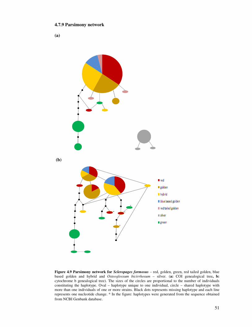
Figure 4.9 Parsimony network for Scleropages formosus – red, golden, green, red tailed golden, blue based golden and hybrid and Osteoglossum bicirrhosum – silver. (a: COI genealogical tree, b: cytochrome b genealogical tree). The sizes of the circles are proportional to the number of individuals constituting the haplotype. Oval – haplotype unique to one individual, circle – shared haplotype with more than one individuals of one or more strains. Black dots represents missing haplotype and each line represents one nucleotide change. * In the figure: haplotypes were generated from the sequence obtained from NCBI Genbank database.

52

The different geographical distributions of red and red tailed gold from

Indonesia, blue base and golden base gold from Malaysia in which the breed purity has

been maintained in the hatchery for commercial purposes were not reflected in the

genetic partitioning, as the Indonesian red and red tailed golden, Malaysian golden base

gold, wild blue base gold largely shared a common ancestral haplotype in COI network

study in Figure 4.9 (a). In Figure 4.9 (b), Cyt b network study also showed the same

haplotype distribution where the red, gold and blue base gold have shared common

ancestral haplotypes.

53

As discussed, DNA barcoding was not able to differentiate stains of Asian

arowana due to its lack of haplotype diversity derived from COI data. It was also

reflected in shallow coalescence in the phylogenetic trees (Figure 4.7, 4.8) as well as

insignificant pairwise population Fst values and exact test of sample non-differentiation

index (Table 4.10, 4.11) except for the gold population in which it showed significant

difference compared to other strains for Cyt b gene (Table 4.11).

The result for this part clearly contradicted the result from the previous study in

which the different strain can be distinguished through different haplotypes that formed

distinct clades on the cytb gene tree (Pouyard et al., 2003). The green strain on the other

hand showed significant differentiation from other strains for both mtDNA and

possesses higher haplotype numbers that are all exclusive to itself (Table 4.8, 4.9).

In the genealogy studies for mtDNA genes, high differentiation was clearly

shown although the differentiation is not high enough for these exclusive haplotypes to

belong to a separate entity as what has been observed in closely related Scleropages.

jardinii, Scleropages leichardti and other outgroups. The distribution of the green

strains on both gene trees raised the possibility that there was genetic structure within

the green strain captive stock due to founder individuals which are taken from different

wild populations and different geographical locations around Malaysia, as previously

reported (Rahman et al., 2008). Although the sample size for the data collection for each

of the strains, especially the red tailed golden and blue base gold strain (n = 3) is small,

increasing the number of samples will increase the number of haplotypes in each

colored strain and reveal more possible shared haplotypes among the strains, but it will

not change the general ancestral haplotype that is commonly shared among various

colored strains. This was corroborated as the same observation was achieved when more

54

sequences (publicly available in GENBANK) were added into the study. It was

hypothesized that each strain of arowana diverged quite recently that it was not reflected

in the COI and cytochrome b mtDNA, as the different strains might not have sufficient

amount of time for these mitochondrial genes to exhibit patterns consistent to the

lineage sorting. The authors agreed that the divergence of each strain could be reflected

in the highly variable mitochondrial regions such as D-loop and the control regions.

55

CHAPTER 5

CONCLUSION

In conclusion, this study showed that there was genetic differentiation especially

in the green strains compared to other strains, but it did not show clear genetic structure

among red and gold strains and their sub-varieties to support emergence of new species

within Scleropages formosus. The result where the green strains formed a paraphyletic

group in both the gene trees also corroborated this conclusion. It was inferred that the

samples collected by Pouyard et al. (2003) were mostly from highly domesticated

stocks, that it failed to capture the largely common haplotype shared among all the

strains.

Our results were incongruent with the taxonomic divisions done by the previous

study (Pouyard et al., 2003). Our genetic relatedness of the different strains also

contradicted with the previous genetic relationship study conducted using microsatellite

data which stated that the genetic distance between red and green is less than between

red and gold (Yue et al., 2002). From this study, it was shown that both COI and

cytocrome b can be good molecular identification markers for Scleropages formosus as

compared to other closely related species. Nevertheless, these markers would not be

suitable to distinguish the different strains of this species except for the green strains.

Therefore, more research should be done using more markers such as D-loop, ND2 and

ATPase to obtain more concrete evidence of the relationship among individuals of

Scleropages formosus.

56

Reference

Avise, J., & Ellis, D. (1986). Mitochondrial DNA and the Evolutionary Genetics of Higher Animals. Philosophical Transactions of the Royal Society of London. Series B, Biological Sciences , 312B, 325-342. Bonde, N. (1979). Paleoenvironment in the “North Sea” as indicated by the fish bearing Mo-clay. Mededelingen Werkgroep voor Tertiaire Kwartaire , 16, 3-16. Boore, J. (1999). Animal mitochondrial genomes. Nucleic Acids Research, 1767-1780. Branicki, W., Kupiec, T., & Pawlowski, R. (2003). Validation of cytochrome b sequence analysis as a method of species identification. J. Forensic Sci , 48, 1-5. Briolay, J., Galtier, N., Brito, R., & Bouvet, Y. (1998). Molecular phylogeny of Cyprinidae inferred from cytochrome b DNA sequences. Mol. Phyl. Evol., , 9, 100-108. Brown, J., Beckenback, K., Beckenback, A., & Smith, M. (1996). Length variation, heteroplasmy, and sequence divergence in the mitochondrial DNA of four species of sturgeon (Acipenser). Genetics , 142, 525-535. Brown, M., Prager, E., Wang, A., & Wilson, A. (1982). Mitochondrial of DNA sequences of primates:tempo and mode of evolution. J Mol Evol , 18, 225-239. Brown, T., Cecconi, C., & Tkachuk, A. (2005). Replication of mitochondrial DNA occurs by strand displacement with alternative light-strand origins, not via a strand-coupled mechanism. Genes and Developmet , 19, 2466-2476. Cantatore, P., & Saccone, C. (1987). Organization, structure, and evolution of mammalian mitochondrial genes. Int. Rev. Cytol , 108, 149-208. Cantatore, P., Roberti, M., Pesole, G., Ludovico, A., Milella, F., Gadaleta, M., et al. (1994). Evolutionary analysis of cytochrome b sequences in some perciformes:evidence for a slower rate of evolution than in mammals. J Mol Evol , 39, 589-597. Castresana, J. (2001). Cytochrome b Phylogeny and the Taxonomy of Great Apes and Mammals. molecular biology and avolution , 465-470. Clare, E., Lim, B., Engstrom, M., Eger, J., & Hebert, P. (2006). DNA barcoding of Neotropical bats: species identification and discovery within Guyana. Molecular Ecology Notes.

57

Clayton, D. (1992). Structure and function of the mitochondrial genome. J. Inherited Metab. Dis , 15, 439-447. Dawes, j., Lim, L., & Cheong, L. (1999). The Dragon Fish. Kingdom Books England. Delin, Q., Taiping, L., Xinquan, Z., Songchang, G., & Junxiang, L. (2006). Mitochondrial cytochromeb Sequence Variation and Phylogenetics of the Highly Specialized Schizothoracine Fishes (Teleostei: Cyprinidae) in the Qinghai-Tibet Plateau. Biochemical Genetics , 44, 270-285. Donald, K., Kenned, Y., & Spencher, H. (2005). The phylogeny and taxonomy of austral monodontine topshells (Mollusca: Gastropoda: Trochidae) inferred from DNA sequences. Molecular Phylogenetics and Evolution , 37, 474-483. Drake, J., Charlesworth, B., Charlesworth, D., & Crow, J. (1998). Rates of spontaneous mutation . Genetics , 148, 1667–1686. Esposti, D., De Vries, S., Crimi, M., Ghelli, A., Patarnello, T., & Meyer, A. (1993). Mitochondrial cytochrome b: evolution and structure of the protein. Biochim Biophys Acta , 1143, 243–271. Excoffier, laval, L., & Schneider, S. (2005). Arlequin ver 3.11:An integrated software package for population genetics data analysis. Evolutionary Bioinformatics Online , 1, 47-55. Gissi, C., Gullberg, A., & Ulfur, A. (1998). The complete mitochondrial DNA sequence of the rabbit, Oryctolagus cuniculs. Genomics , 50, 161-169. Goh, W., & Chua, J. (1999). The Asian Arowana. Dragon fish industry,singapore. Groves, P., & Shields, G. (1996). Phylogenetics of the Caprinae on cytochrome b sequce. Mol.Phyl.Evol , 5, 467-476. Gyllestein, U., Wharton, D., Josefsson, A., & Wilson, A. (1991). Paternal inheritance of mitochondrial DNA in mice. Nature , 352, 255-257. Hajibabaei, M., Janzen, D., Burns, J., Hallwachs, W., & Hebert, P. (2006). DNA barcodes distinguish species of tropical Lepidoptera. Evolution, 103, 968 –971.

58

Härlid, A., Janke, A., & Árnason, U. (1998). The complete mitochondrial genome of Rhea americana and early avian divergences. J. Mol. Evol , 46. Hayashi, J., Tagashira, Y., & Yoshida, M. (1985). Absence of extensive recombination between interspecies and intraspecies mitochodrial DNA in mammalian cells. Exp. Cell Res , 160, 387-395. Hebert, P., Cywinska, A., Ball, S., & Dewaard, J. (2003). biological identification through DNA barcodes. Proceeding of the Royal Society of london , 313-322. Hebert, P., Stoeckle, M., Zemlak, T., & Francis, C. (2004). Identification of Birds through DNA Barcodes. PLoS Biol , 2, 1657–1663. Hu, Y., Mu, X., Wang, X., Liu, C., Wang, P., & Luo, J. (2009). Preliminary Study on Mitochondrial DNA Cytochrome B Sequences and. Internationl journal of biology , 1, 28-32. Hubert, N., Hanner, R., Holm, E., Mandrak, N., & Taylor, E. (2008). Identifying Canadian Freshwater Fishes through DNA Barcodes. PLoS ONE , 3 (6), e2490. Inoue, J., Miya, M., Tsukamoto, K., & Nishida, M. (2001). A mitogenomic perspective on the basal teleostean phylogeny: resolving higher level relationships with longer DNA sequences. Mol Phylogenet Evol , 20, 275-285. Irwin, D., Kocher, T., & Wilson, A. (1991). Evolution of the cytochrome b gene of mammals. J.Mol.Evol , 32, 128-144. Jarne, P., & Lagoda, J. (1996). Microsatellites, from molecules to populations and back. Trends in Ecology and Evolution , 11, 424-429. Jhons, G., & Avise, J. (1998). A comparative summary of genetic distance in the vertebrate from the mitochondrial cytochrome b gene. Molecular Biology and Evolution ,15, 1481-1490. Joseph, J., Evans, D., & Broad, S. (1986). International trade in Asian Bonytongues. Traffic Bulletin , 3, 73-76. Kondo, R., Satta, Y., Matsuura, E., Ishiwa, H., Takahata, N., & Chigusa, S. (1990). Incomplete maternal transmission of mitochondrial DNA in Drosophila. Genetics , 126, 657-663.

59

Kottelat, M. (1996). Scleropages formosus. (2006). IUCN Red List of Threatened Species. IUCN 2006. Kottelat, M., Whitten, A., Kartikasari, S., & Wirjoatmodjo, S. (1993). Freshwater fishes of Western Indonesia and Sulawesi. Hong Kong: Periplus Editions. Kumazawa, Y., & Nishida, M. (2000). Molecular phylogeny of Osteoglossoids a new model for Gondwanian origin and plate tectonic transportation of the Asian arowana. Mol Biol Evol , 17 (2), 1869-1878. Kyle, C., & Wilson, C. (2006). Mitochondrial DNA identification of game and harvested freshwater fish species. Forensic Science International , 166, 68–76. Ludwing, A., Debus, L., & Jenneckens, I. (2002). A molecular approach to control the international trade in black caviar. International review of hydrobiology , 661-674. Lydeard, C., & Roe, K. (1997). the phylogenetic utility of the mitochondria cytochrome b gene for inferring relationships among Actinopterygian fishes. In T. Kocher, & C. Stepien, molecular systematics of fish (pp. 285-303). New York: Academic Press. Machordom, A., Araujo, R., Erpenbeck, D., & Ramos, M. (2003). Phylogeography and conservation genetics of endangered European Margaritiferidae (Bivalvia: Unionoidea). Biological Journal of the Linnean Society , 78, 235-252. Mayer, A. (1993). Evolution of mitochondrial DNA in fishes. biochemistry and molecular biology of fishes , 1-38. Mayer, A. (1994). Shortcoming of the cytochrome b gene as a molecular marker. Trend Ecol Evol , 9, 278-280. Meyer, A., & Wilson, C. (1990). Origin of tetrapods inferred from their mitochondrial DNA affiliation to lungfish. J Mol Evol , 31, 359-364. Muller, S., & Schlegel, H. (n.d.). Beschrijving van een’ nieuwen Zoetwater-visch van Borneo, Osteoglossum formosum. Murray, B., McClymont, R., & Strobeck, C. (1995). Forensic identification ofungulate species using restriction digests of PCR-amplified mitochondrial DNA. J. Forensic Sci , 40, 943–951.

60

Nelson, J. (1994). Fishes of the World. New York: Wiley. Ng, H., & Tan, H. (1999). The fishes of the Endau Drainage, Peninsular Malaysia with description of two new species of catfishes (Teleostei: Akysidae, Bagridae). Zoological Studies , 38, 350-366. Persis, M., Chandra Sekhar Reddy, A., Rao, L., Khedkar, G., Ravinder, K., & Nasruddin, K. (2008). COI (cytochrome oxidase-I) sequence based studies of Carangid fishes from Kakinada coast, India. Molecular Biology Reports , 1733-1740. Pouyaud, L., Sudarto, & Teugels, G. (2003). The different colour varieties of the Asian arowana Scleropages formosus (Osteoglossidae) are distinct species: Morphologic and genetic evidences. Cybium , 27, 287-305. Queller, D., Strassmann, J., & Hughes, C. (1993). Microsatellites and kinship. Trends in Ecology and Evolution , 8, 285. Rubinoff, D., Cameron, S., & Will, K. (2006). A Genomic Perspective on the Shortcomings of Mitochondrial DNA for ‘‘Barcoding’’ Identification. Journal of Heredity , 97, 581–594. Scott, D., & Fuller, J. (1976). The reproductive biology of Scleropages formosus (Muller & Schlegel) (Osteoglossomorpha, Osteoglossidae) in Malaya, and the morphology of its pituitary. J Fish Biol , 8, 48-53. Sérgio, L. P. (2000). Mitochondrial genome organization and vertebrate phylogenetics. Genetics and Molecular Biology , 23, 745-752. Smith, P., Mcveagh, S., Won, Y., & Vrijenhoek, R. (2004). Genetic heterogeneity among New Zealand species of hydrothermal vent mussels (Mytilidae: Bathymodiolus). Marine Biology , 144, 537-545. Stearn, C., Carroll, R., & Clark, T. (1979). Geological Evolution of North. NY: John Wiley and Sons. Strachan, T., & Read, A. (1999). Human Molecular Genetics 2. Newcastle: John Wiley & Sons. Strauss, R., & Bond, C. (1990). Taxonomic methods: morphology. In: Schreck CB, Moyle PB (eds) Methods for fish biology. Maryland: American Fisheries Society.

61

Suleiman, M. Z. (1999). Pembiakan Ikan Arowana, Scleropages formosus (Muller and Schlegel). Risalah Perikanan . Jabatan Perikanan Malaysia , 67, 17. Tamura, K., Dudley, J., Nei, M., & Kumar, S. (2007). MEGA4: Molecular Evolutionary Genetics Analysis (MEGA) software version 4.0. Molecular Biology and evolution , 24, 1596-1599. Tang, P. (2004). Population and phylogenetic studies on Asian Arowana (Scleropages formosus). kl, malaysia: uniiversity of malaya. Tang, P., Sivananthan, J., Pillay, S., & Muniandy, S. (2004). Genetic Structure and Biogeography of Asian Arowana (Scleropages formosus) determined by Microsatellite and Mitochondrial DNA analysis. Asian Fisheries Science , 17, 81-92. Teletchea, F. (2009). Molecular identification methods of fish species: reassessment and possible applications. Reviews in Fish Biology and Fisheries , 265-293. Thompson, J., Gibson, T., Plewniak, F., & Higgins, D. (1997). The CLUSTAL_X windows interface: flexible strategies for multiple sequence alignment aided by quality analysis tools. Nucleic Acids Res. , 24, 4876-82. Ursing, B., & Arnason, U. (1998). The complete mitochondrial DNA sequence of the pig (Sus scrofa). J. Mol. Evol , 47, 302-306. Ward, R., Woodwark, M., & Skibinski, D. (1994). A comparison of genetic diversity levels in marine, freshwater, and anadromous fishes. Journal of fish biology , 213-232. Ward, R., Zemlak, T., Innes, B., Last, P., & Hebert, P. (2005). DNA barcoding of Australia’s fish species. Philosophical Transactions of the Royal Society, Series B , 360, 1847–1857. Ward, R., Zemlak, T., Innes, B., Last, P., & Hebert, P. (2005). DNA barcoding of Australia's fish species. Phil. Trans. R. Soc. B , 1847-1857. Waugh, J. (2007). DNA barcoding in animal species:progress, potential and pitfalls. Phylogenetics and systematics , 188–197. Wen-Feng, l., Chyuan-Yuan, S., & Deng-Fwu, H. (2005). Identification of Four Thunnus Tuna Species Using Mitochondrial Cytochrome b Gene Sequence and PCR-RFLP Analysis. Food and drug analysis, 382-388.

62

Yann, S., Bonnefoy, N., Jean, P., Chiron, S., & Dujardin, G. (2002). A phatogenic cytochrome b mutation reveals new interactions between subunits of the mitochondrial bc1 complex. J.Biol.Chem . Yue, G., Liew, W., & Orban, l. (2006). The complete mitochondrial genome of a basal teleost, the Asian arowana (Scleropages formosus, Osteoglossidae). BMC Genomics , 7, 242.

63

APPENDIX A

Figur A1: Malaysian Green Arowana,

http://arowana168.co.uk/wp-content/uploads/2009/06/green-arowana-500x238.jpg

Figure A2: Indonesian Gold Arowana

http://wb3.itrademarket.com/pdimage/64/1231364_img_6565.jpg

64

Figure A3: Indonesian Red Arowana

http://arowana168.co.uk/wp-content/uploads/2009/06/G1R-500x180.jpg

Figure A4: Indonesian red- tail Gold Arowana

http://arowana168.co.uk/wp-content/uploads/2009/06/red-tail-golden-arowana-500x294.jpg

Figure A5: Silver Arowana

http://www.aqua-fish.net/imgs/fish/silver-arowana-profile.jpg

65

APPENDIX B

List of out groups used in this study

Scientific

name

Accesses

number

Database

URL

1.Arapaima

gigas (COI)

EF523611 Nucleotide Collection (nr/nt)

http://www.ncbi.nlm.nih.gov/nuccore/146221455?report=GenBank

2.Scleropages

jardinii

AB035236 Nucleotide Collection (nr/nt)

http://www.ncbi.nlm.nih.gov/nuccore/11862847?report=GenBank

3.Scleropages

leichardti

AB035237 Nucleotide Collection (nr/nt)

http://www.ncbi.nlm.nih.gov/nuccore/11862849?report=GenBank

4.Osteoglossum

bicirrhosum

AB035238 Nucleotide Collection (nr/nt)

http://www.ncbi.nlm.nih.gov/nuccore/11862851?report=GenBank

5.Osteoglossum

ferreirai

AB035239.1 Nucleotide Collection (nr/nt)

http://www.ncbi.nlm.nih.gov/nuccore/11862853?report=GenBank

6.Arapaima

gigas (cytb)

AB035241.1 Nucleotide Collection

(nr/nt)

http://www.ncbi.nlm.nih.gov/nuccore/11862857?report=GenBank

7.Heterotis

niloticus

AB035240.1 Nucleotide Collection

(nr/nt)

http://www.ncbi.nlm.nih.gov/nuccore/11862855?report=GenBank

66

APPENDIX C

COI sequences of 12 hoplotypes from Arowana’s strains used in this study. Identity

with the reference sequences is indicated by dots.

Hap 1 G T C G G T A C T G C C C T C A G C C T C C T A A T C C G C

Hap 2 . . . . . . . . . . . . . . . . . . . . . . . . . . . . . .

Hap 3 . . . . . . . . . . . . . . . . . . . . . . . . . . . . . .

Hap 4 . . . . . . . . . . . . . . . . . . . . . . . . . . . . . .

Hap 5 . . . . . . . . . . . . . . . . . . . . . . . . . . . . . .

Hap 6 . . . . . . . . . . . . . . . . . . . . . . . . . . . . . .

Hap 7 . . . . . . . . . . . . . . . . . . . . . . . . . . . . . .

Hap 8 . . T . . C . . C . . T . . T . . . . . T . . G . . T . . .

Hap 9 . . T . . C . . C . . T . . T . . . . . T . . G . . T . . .

Hap 10 . . T . . C . . C . . T . . T . . . . . T . . G . . T . . .

Hap 11 . . . . . . . . . . . . . . . . . . . . . . . . . . . . . .

Hap 12 . . . . . . . . . . . . . . . . . . . . . . . . . . . . . .

Hap 1 G C A G A A C T A A G C C A G C C T G G A G C C C T C C T T

Hap 2 . . . . . . . . . . . . . . . . . . . . . . . . . . . . . .

Hap 3 . . . . . . . . . . . . . . . . . . . . . . . . . . . . . .

Hap 4 . . . . . . . . . . . . . . . . . . . . . . . . . . . . . .

Hap 5 . . . . . . . . . . . . . . . . . . . . . . . . . . . . . .

Hap 6 . . . . . . . . . . . . . . . . . . . . . . . . . . . . . .

Hap 7 . . . . . . . . . . . . . . . . . . . . . . . . . . . . . .

Hap 8 . . . . . . . . C . . . . . A . . . . . . T . . T . G . . .

Hap 9 . . . . . . . . C . . . . . A . . . . . . T . . T . G . . .

Hap 10 . . . . . . . . C . . . . . A . . . . . . T . . T . G . . .

Hap 11 . . . . . . . . . . . . . . . . . . . . . . . . . . . . . .

Hap 12 . . . . . . . . . . . . . . . . . . . . G . . . . . . . . .

Hap 1 G G T G A C G A C C A A A T C T A T A A T G T T A T C G T A

Hap 2 . . . . . . . . . . . . . . . . . . . . . . . . . . . . . .

Hap 3 . . . . . . . . . . . . . . . . . . . . . . . . . . . . . .

Hap 4 . . . . . . . . . . . . . . . . . . . . . . . . . . . . . .

Hap 5 . . . . . . . . . . . . . . . . . . . . . . . . . . . . . .

Hap 6 . . . . . . . . . . . . . . . . . . . . . . . . . . . . . .

Hap 7 . . . . . . . . . . . . . . . . . . . . . . . . . . . . . .

Hap 8 . . . . . T . . T . . . . . T . . . . . . . . C . . . . . C

Hap 9 . . . . . T . . T . . . . . T . . . . . . . . C . . . . . C

Hap 10 . . . . . T . . T . . . . . T . . . . . . . . C . . . . . C

Hap 11 . . . . . . . . . . . . . . . . . . . . . . . . . . . . . .

Hap 12 . . . . . . . . . . . . . . . . . . . . . . . . . . . . . .

Hap 1 A C A G C A C A C G C T T T C G T A A T A A T T T T C T T C

Hap 2 . . . . . . . . . . . . . . . . . . . . . . . . . . . . . .

Hap 3 . . . . . . . . . . . . . . . . . . . . . . . . . . . . . .

Hap 4 . . . . . . . . . . . . . . . . . . . . . . . . . . . . . .

Hap 5 . . . . . . . . . . . . . . . . . . . . . . . . . . . . . .

Hap 6 . . . . . . . . . . . . . . . . . . . . . . . . . . . . . .

Hap 7 . . . . . . . . . . . . . . . . . . . . . . . . . . . . . .

Hap 8 . . . . . . . . T . . . . . T . . . . . G . . . . . . . . .

Hap 9 . . . . . . . . T . . . . . T . . . . . G . . . . . . . . .

Hap 10 . . . . . . . . T . . . . . T . . . . . G . . . . . . . . .

Hap 11 . . . . . . . . . . . . . . . . . . . . . . . . . . . . . .

67

Hap 12 . . . . . . . . . . . . . . . . . . . . . . . . . . . . . .

Hap 1 A T G G T C A T G C C A A T T A T A A T T G G G G G C T T T

Hap 2 . . . . . . . . . . . . . . . . . . . . . . . . . . . . . .

Hap 3 . . . . . . . . . . . . G . . . . . . . . . . . . . . . . .

Hap 4 . . . . . . . . . . . . . . . . . . . . . . . . . . . . . .

Hap 5 . . . . . . . . . . . . . . . . . . . . . . . . . . . . . .

Hap 6 . . . . . . . . . . . . . . . . . . . . . . . . . . . . . .

Hap 7 . . . . . . . . . . . . . . . . . . . . . . . . . . . . . .

Hap 8 . . A . . A . . A . . . . . . . . . . . C . . C . . A . . .

Hap 9 . . A . . A . . A . . . . . . . . . . . C . . C . . A . . .

Hap 10 . . A . . A . . A . . . . . . . . . . . C . . C . . A . . .

Hap 11 . . . . . . . . . . . . . . . . . . . . . . . . . . . . . .

Hap 12 . . . . . . . . . . . . . . . . . . . . . . . . . . . . . .

Hap 1 G G C A A C T G A C T A G T C C C A C T T A T G A T C G G A

Hap 2 . . . . . . . . . . . . . . . . . . . . . . . . . . . . . .

Hap 3 . . . . . . . . . . . . . . . . . . . . . . . . . . . . . .

Hap 4 . . . . . . . . . . . . . . . . . . . . . . . . . . . . . .

Hap 5 . . . . . . . . . . . . . . . . . . . . . . . . . . . . . .

Hap 6 . . . . . . . . . . . . . . . . . . . . . . . . . . . . . .

Hap 7 . . . . . . . . . . . . . . . . . . . . . . . . . . . . . .

Hap 8 . . T . . . . . . . . T A . T . . . . . G . . A . . . . . T

Hap 9 . . T . . . . . . . . T A . T . . . . . G . . A . . . . . T

Hap 10 . . T . . . . . . . . T A . T . . . . . G . . A . . . . . T

Hap 11 . . . . . . . . . . . . . . . . . . . . . . . . . . . . . .

Hap 12 . . . . . . . . . . . . . . . . . . . . . . . . . . . . . .

Hap 1 G C C C C A G A C A T A G C A T T C C C G C G A A T A A A C

Hap 2 . . . . . . . . . . . . . . . . . . . . . . . . . . . . . .

Hap 3 . . . . . . . . . . . . . . . . . . . . . . . . . . . . . .

Hap 4 . . . . . . . . . . . . . . . . . . . . . . . . . . . . . .

Hap 5 . . . . . . . . . . . . . . . . . . . . . . . . . . . . . .

Hap 6 . . . . . . . . . . . . . . . . . . . . . . . . . . . . . .

Hap 7 . . . . . . . . . . . . . . . . . . . . . . . . . . . . . .

Hap 8 . . . . . . . . . . . . . . T . . . . . C . . . . . . . . .

Hap 9 . . . . . . . . . . . . . . T . . . . . C . . . . . . . . .

Hap10 . . . . . . . . . . . . . . T . . . . . C . . . . . . . . .

Hap 11 . . . . . . . . . . . . . . . . . . . . . . . . . . . . . .

Hap 12 . . . . . . . . . . . . . . . . . . . . . . . . . . . . . .

Hap 1 A A C A T A A G C T T C T G G C T T C T A C C C C C T T C C

Hap 2 . . . . . . . . . . . . . . . . . . . . . . . . . . . . . .

Hap 3 . . . . . . . . . . . . . . . . . . . . . . . . . . . . . .

Hap 4 . . . . . . . . . . . . . . . . . . . . . . . . . . C . . .

Hap 5 . . . . . . . . . . . . . . . . . . . . . . . . . . C . . .

Hap 6 . . . . . . . . . . . . . . . . . . . . . . . . . . . . . .

Hap 7 . . . . . . . . . . . . . . . . . . . . . . . . . . . . . .

Hap 8 . . T . . G . . T . . T . . A . . A . . G . . G . . . . . A

Hap 9 . . T . . G . . T . . T . . A . . A . . G . . G . . . . . A

Hap 10 . . T . . G . . T . . T . . A . . A . . G . . G . . . . . A

Hap 11 . . . . . . . . . . . . . . . . . . . . . . . . . . . . . .

Hap 12 . . . . . . . . . . . . . . . . . . . . . . . . . . . . . .

Hap 1 T T C T T A C T C C T C T T G G C C T C T T C C G G A G T A

Hap 2 . . . . . . . . . . . . . . . . . . . . . . . . . . . . . .

Hap 3 . . . . . . . . . . . . . . . . . . . . . . . . . . . . . .

68

Hap 4 . . . C . . . . . . . . . . . . . . . . . . . . . . . . . .

Hap 5 . . . . . . . . . . . . . . . . . . . . . . . . . . . . . .

Hap 6 . . . . . . . . . . . . . . . . . . . . . . . . . . . . . .

Hap 7 . . . . . . . . . . . . . . . . . . . . . . . . . . . . . .

Hap 8 . . . C . C . . T . . T . . A . . . . . A . . T . . G . . .

Hap 9 . . . C . C . . T . . T . . A . . . . . A . . T . . G A . .

Hap 10 . . . C . C . . T . . T . . A . . . . . A . . T . . G . . .

Hap 11 . . . . . . . . . . . . . . . . . . . . . . . . . . . . . .

Hap 12 . . . . . . . . . . . . . . . . . . . . . . . . . . . . . .

Hap 1 G A A G C A G G G G C T G G A A C A G G A T G G A C G G T T

Hap 2 . . . . . . . . . . . . . . . . . . . . . . . A . . . . . .

Hap 3 . . . . . . . . . . . . . . . . . . . . . . . A . . . . . .

Hap 4 . . . . . . . . . . . . . . . . . . . . . . . A . . . . . .

Hap 5 . . . . . . . . . . . . . . . . . . . . . . . A . . . . . .

Hap 6 . . . . . . . . . . . . . . . . . . . . . . . . . . . . . .

Hap 7 . . . . . . . . . . . . . . . . . . . . . . . . . . . . . .

Hap 8 . . . . . T . . T . . A . . . . . . . . . . . A . . T . . A

Hap 9 . . . . . T . . T . . A . . . . . . . . . . . A . . T . . A

Hap 10 . . . . . T . . T . . A . . . . . . . . . . . A . . T . . A

Hap 11 . . . . . . . . . . . . . . . . . . . . . . . A . . . . . .

Hap 12 . . . . . . . . . . . . . . . . . . . . . . . A . . . . . .

Hap 1 T A C C C C C C T C T A G C G G G T A A T C T G G C C C A T

Hap 2 . . . . . . . . . . . . . . . . . . . . . . . . . . . . . .

Hap 3 . . . . . . . . . . . . . . . . . . . . . . . . . . . . . .

Hap 4 . . . . . . . . . . . . . . . . . . . . . . . . . . . . . C

Hap 5 . . . . . . . . . . . . . . . . . . . . . . . . . . . . . C

Hap 6 . . . . . . . . . . . . . . . . . . . . . . . . . . . . . .

Hap 7 . . . . . . . . . . . G . . . . . . . . . . . . . . . . . .

Hap 8 . . . . . A . . . T . . . . A . . A . . C . . A . . A . . .

Hap 9 . . . . . A . . . T . . . . A . . A . . C . . A . . A . . .

Hap 10 . . . . . A . . . T . . . . A . . A . . C . . A . . A . . .

Hap 11 . . . . . . . . . . . . . . . . . . . . . . . . . . . . . .

Hap 12 . . . . . . . . . . . . . . . . . . . . . . . . . . . . . .

Hap 1 G C C G G A G C A T C C G T A G A T C T A A C T A T T T T T

Hap 2 . . . . . . . . . . . . . . . . . . . . . . . . . . . . . .

Hap 3 . . . . . . . . . . . . . . . . . . . . . . . . . . . . . .

Hap 4 . . . . . . . . . . . . . . . . . . . . . . . . . . . . . .

Hap 5 . . . . . . . . . . . . . . . . . . . . . . . . . . . . . .

Hap 6 . . . . . . . . . . . . . . . . . . . . . . . . . . . . . .

Hap 7 . . . . . . . . . . . . . . . . . . . . . . . . . . . . . .

Hap 8 . . A . . . . . . . . . . . C . . C T . . . . . . . C . . .

Hap 9 . . A . . . . . . . . . . . C . . C T . . . . . . . C . . .

Hap 10 . . A . . . . . . . . . . . C . . C T . . . . . . . C . . .

Hap 11 . . . . . . . . . . . . . . . . . . . . . . . . . . . . . .

Hap 12 . . . . . . . . . . . . . . . . . . . . . . . . . . . . . .

Hap 1 T C T T T A C A C C T G G C T G G A G T C T C A T C C A T C

Hap 2 . . . . . . . . . . . . . . . . . . . . . . . . . . . . . .

Hap 3 . . . . . . . . . . . . . . . . . . . . . . . . . . . . . .

Hap 4 . . . . . . . . . . . . . . . . . . . . . . . . . . . . . .

Hap 5 . . . . . . . . . . . . . . . . . . . . . . . . . . . . . .

Hap 6 . . . . . . . . . . . . . . . . . . . . . . . . . . . . . .

Hap 7 . . . . . . . . . . . . . . . . . . . . . . . . . . . . . .

Hap 8 . . A C . . . . T . . . . . A . . T . . T . . . . . T . . T

69

Hap 9 . . A C . . . . T . . . . . A . . T . . T . . . . . T . . T

Hap 10 . . A C . . . . T . . . . . A . . T . . T . . . . . T . . T

Hap 11 . . . . . . . . . . . . . . . . . . . . . . . . . . . . . .

Hap 12 . . . . . . . . . . . . . . . . . . . . . . . . . . . . . .

Hap 1 C T C G G G G C A A T T A A C T T T A T T A C C A C T A T T

Hap 2 . . . . . . . . . . . . . . . . . . . . . . . . . . . . . .

Hap 3 . . . . . . . . . . . . . . . . . . . . . . . . . . . . . .

Hap 4 . . . . . A . . . . . C . . . . . . . . . . . T . . . . . .

Hap 5 . . . . . A . . . . . C . . . . . . . . . . . . . . . . . .

Hap 6 . . . . . . . . . . . . . . . . . . . . . . . . . . . . . .

Hap 7 . . . . . . . . . . . . . . . . . . . . . . . . . . . . . .

Hap 8 T . A . . . . . . . . . . . T . . . . . . . . T . . A . . C

Hap 9 T . A . . . . . . . . . . . T . . . . . . . . T . . A . . C

Hap 10 T . A . . . . . . . . . . . T . . . . . . . . T . . A . . C

Hap 11 . . . . . . . . . . . . . . . . . . . . . . . . . . . . . .

Hap 12 . . . . . . . . . . . . . . . . . . . . . . . . . . . . . .

Hap 1 A T T A A C A T A A A A C C C C C A G C C A T T A C C C A A

Hap 2 . . . . . . . . . . . . . . . . . . . . . . . . . . . . . .

Hap 3 . . . . . . . . . . . . . . . . . . . . . . . . . . . . . .

Hap 4 . . . . . . . . . . . . . . . . . . . . . . . . . . . . . .

Hap 5 . . . . . . . . . . . . . . . . . . . . . . . . . . . . . .

Hap 6 . . . . . . . . . . . . . . . . . . . . . . . . . . . . . .

Hap 7 . . . . . . . . . . . . . . . . . . . . . . . . . . . . . .

Hap 8 . . C . . T . . G . . G . . . . . T . . . . . C . . T . . .

Hap 9 . . C . . T . . G . . G . . . . . T . . . . . C . . T . . .

Hap 10 . . C . . T . . G . . G . . . . . T . . . . . C . . T . . .

Hap 11 . . . . . . . . . . . . . . . . . . . . . . . . . . . . . .

Hap 12 . . . . . . . . . . . . . . . . . . . . . . . . . . . . . .

Hap 1 T A C C A A A C A C C T C T A T T T G T C T G A T C T G T T

Hap 2 . . . . . . . . . . . . . . . . . . . . . . . . . . . . . C

Hap 3 . . . . . . . . . . . . . . . . . . . . . . . . . . . . . C

Hap 4 . . . . . . . . . . . . . . . . . . . . . . . . . . . . . .

Hap 5 . . . . . . . . . . . . . . . . . . . . . . . . . . . . . .

Hap 6 . . . . . . . . . . . . . . . . . . . . . . . . . . . . . C

Hap 7 . . . . . . . . . . . . . . . . . . . . . . . . . . . . . C

Hap 8 . . . . . . . . . . . . . . G . . . A . . . . . . . C . . C

Hap 9 . . . . . . . . . . . . . . G . . . A . . . . . . . C . . C

Hap 10 . . . . . . . . . . . . . . G . . . A . . . . . . . C . . C

Hap 11 . . . . . . . . . . . . . . . . . . . . . . . . . . . . . C

Hap 12 . . . . . . . . . . . . . . . . . . . . . . . . . . . . . C

Hap 1 C T A G T A A C C G C T G T C C T T C T A C T T C T C T C C

Hap 2 . . . . . . . . . . . . . . . . . . . . . . . . . . . . . .

Hap 3 . . . . . . . . . . . . . . . . . . . . . . . . . . . . . .

Hap 4 . . . . . . . . . . . . . . . . . . . . . . . . . . . . . .

Hap 5 . . . . . . . . . . . . . . . . . . . . . . . . . . . . . .

Hap 6 . . . . . . . . . . . . . . . . . . . . . . . . . . . . . .

Hap 7 . . . . . . . . . . . . . . . . . . . . . . . . . . . . . .

Hap 8 . . . . . . . . T . . A . . . . . . . . T . . C . . T . . T

Hap 9 . . . . . . . . T . . A . . . . . . . . T . . C . . T . . T

Hap 10 . . . . . . . . T . . A . . . . . . . . T . . C . . T . . T

Hap 11 . . . . . . . . . . . . . . . . . . . . . . . . . . . . . .

Hap 12 . . . . . . . . . . . . . . . . . . . . . . . . . . . . . .

70

Hap 1 C T C C C A G T C T T A G C T G C A G G A A T C A C T A T A

Hap 2 . . . . . . . . . . . . . . . . . . . . . . . . . . . . . .

Hap 3 . . . . . . . . . . . . . . . . . . . . . . . . . . . . . .

Hap 4 . . . . . . . . . . . . . . . . . . . . . . . . . . . . . .

Hap 5 . . . . . . . . . . . . . . . . . . . . . . . . . . . . . .

Hap 6 . . . . . . . . . . . . . . . . . . . . . . . . . . . . . .

Hap 7 . . . . . . . . . . . . . . . . . . . . . . . . . . . . . .

Hap 8 . . T . . . . . . . . . . . . . . . . . T . . T . . A . . .

Hap 9 . . T . . . . . . . . . . . . . . . . . T . . T . . A . . .

Hap 10 . . T . . . . . . . . . . . . . . . . . T . . T . . A . . .

Hap 11 . . . . . . . . . . . . . . . . . . . . . . . . . . . . . .

Hap 12 . . . . . . . . . . . . . . . . . . . . . . . . . . . . . .

Hap 1 C T T C T A A C A G A T C G C A A C C T T A A C A C C A C A

Hap 2 . . . . . . . . . . . . . . . . . . . . . . . . . . . . . .

Hap 3 . . . . . . . . . . . . . . . . . . . . . . . . . . . . . .

Hap 4 . . . . . . . . . . . . . . . . . . . . . . . . . . . . . .

Hap 5 . . . . . . . . . . . . . . . . . . . . . . . . . . . . . .

Hap 6 . . . . . . . . . . . . . . . . . . . . . . . . . . . . . .

Hap 7 . . . . . . . . . . . . . . . . . . . . . . . . . . . . . .

Hap 8 . . . T . . . . . . . C . . T . . . T . A . . . . . T . . T

Hap 9 . . . T . . . . . . . C . . T . . . T . A . . . . . T . . T

Hap 10 . . . T . . . . . . . C . . T . . . T . A . . . . . T . . T

Hap 11 . . . . . . . . . . . . . . . . . . . . . . . . . . . . . .

Hap 12 . . . . . . . . . . . . . . . . . . . . . . . . . . . . . .

Hap 1 T T C T T T G A C C C A G C T G G G G G A G G G G A T C C A

Hap 2 . . . . . . . . . . . . . . . . . . . . . . . . . . . . . .

Hap 3 . . . . . . . . . . . . . . . . . . . . . . . . . . . . . .

Hap 4 . . . . . . . . . . . . . . . . . . . . . . . A . . . . . .

Hap 5 . . . . . . . . . . . . . . . . . . . . . . . A . . . . . .

Hap 6 . . . . . . . . . . . . . . . . . . . . . . . . . . . . . .

Hap 7 . . . . . . . . . . . . . . . . . . . . . . . . . . . . . .

Hap 8 . . . . . C . . . . . . . . . . . . . . . . . . . . C . . .

Hap 9 . . . . . C . . . . . . . . . . . . . . . . . . . . C . . .

Hap 10 . . . . . C . . . . . . . . . . . . . . . . . . . . C . . .

Hap 11 . . . . . . . . . . . G . . . . . . . . . . . . . . . . . .

Hap 12 . . . . . . . . . . . . . . . . . . . . . . . . . . . . . .

Hap 1 A T C C T A T A T C A A C A C C T A T T C T G A

Hap 2 . . . . . . . . . . . . . . . . . . . . . . . .

Hap 3 . . . . . . . . . . . . . . . . . . . . . . . .

Hap 4 . . . . . . . . . . . . . . . . . . . . . . . .

Hap 5 . . . . . . . . . . . . . . . . . . . . . . . .

Hap 6 . . . . . . . . . . . . . . . . . . . . . . . .

Hap 7 . . . . . . . . . . . . . . . . . . . . . . . .

Hap 8 . . . . . . . . . . . . . . . T . . . . . . . .

Hap 9 . . . . . . . . . . . . . . . T . . . . . . . .

Hap 10 . . . . . . . . . . . . . . . T . . . . A . . .

Hap 11 . . . . . . . . . . . . . . . . . . . . . . . .

Hap 12 . . . . . . . . . . . . . . . . . . . . . . . .

71

APPENDIX C

1) Cyt b sequences of 10 hoplotypes from Arowana’s strain used in this study.

Identity with the reference sequences is indicated by dots.

Hap 1 A T G G C C A G C C T C C G A A A A A C C C A C C C A A T C

Hap 2 . . . . . . . . . . . . . . . . . . . . . . . . . . . . . .

Hap 3 . . . . . . . . . . . . . . . . . . . . . . . . . . . . . .

Hap 4 . . . . . . . . . . . . . . . . . . . . . . . . . . . . . .

Hap 5 . . . . . . . . . . . . . . . . . . . . . . . . . . . . . .

Hap 6 . . . . . . . . . . . . . . . . . . . . . . . . . . . . . .

Hap 7 . . . . . . . . . . . . . . . . . . . . . . . . . . . . . .

Hap 8 . . . . . . . . . . . . . . . . . . . . . . . . . . . . . .

Hap 9 . . . . . . . . . . . . . . . . . . . . . . . . . . . . . .

Hap 10 . . . . . . . . . . . . . . . . . . . . . . . . . . . . . .

Hap 1 G C C A A A A T C A T A A A C G A C G C C C T T G T T G A C

Hap 2 . . . . . . . . . . . . . . . . . . . . . . . . . . . . . .

Hap 3 . . . . . . . . . . . . . . . . . . . . . . . . . . . . . .

Hap 4 . . . . . . . . . . . . . . . . . . . . . . . . . . . . . .

Hap 5 . . . . . . . . . . . . . . . . . . . . . . . . . . . . . .

Hap 6 . . . . . . . . . . . . . . . . . . . . . . . . . . . . . .

Hap 7 . . . . . . . . . . . . . . . . . . . . . . . . . . . . . .

Hap 8 . . . . . . . . . . . . . . . . . . . . . . . . . . . . . .

Hap 9 . . . . . . . . . . . . . . . . . . . . . . . . . . . . . .

Hap 10 . . . . . . . . . . . . . . . . . . . . . . . . . . . . . .

Hap 1 C T C C C A A C A C C A T C C A A C A T T T C C G C C T G A

Hap 2 . . . . . . G . . . . . . . . . . . . . . . . . . . . . . .

Hap 3 . . . . . . G . G . . . . . . . . . . . . . . . . . . . . .

Hap 4 . . . . . . G . G . . . . . . . . . . . . . . . . . . . . .

Hap 5 . . . . . . G . G . . . . . . . . . . . . . . . . . . . . .

Hap 6 . . . . . . G . G . . . . . . . . . . . . . . . . . . . . .

Hap 7 . . . . . . G . G . . . . . . . . . . . . . . . . . . . . .

Hap 8 . . . . . . G . G . . . . . . . . . . . . . . . . . . . . .

Hap 9 . . . . . . . . G . . . . . . . . . . . . . . . . . . . . .

Hap 10 . . . . . . G . G . . . . . . . . . . . . . . . . . . . . .

Hap 1 T G A A A C T T C G G C T C C C T T C T A G G C C T C T G C

Hap 2 . . . . . . . . . . . . . . . . . . . . . . . . . . . . . .

Hap 3 . . . . . . . . . . . . . . . . . . . . . . . . . . . . . .

Hap 4 . . G . . . . . . . . . . . . . . . . . . . . . . . . . . .

Hap 5 . . G . . . . . . . . . . . . . . . . . . . . . . . . . . .

Hap 6 . . G . . . . . . . . . . . . . . . . . . . . . . . . . . .

Hap 7 . . G . . . . . . . . . . . . . . . . . . . . . . . . . . .

Hap 8 . . G . . . . . . . . . . . . . . . . . . . . . . . . . . .

Hap 9 . . G . . . . . . . . . . . . . . . . . . . . . . . . . . .

Hap 10 . . G . . . . . . . . . . . . . . . . . . . . . . . . . . .

Hap 1 C T G G G G G C C C A A A T T C T A A C A G G C C T C T T C

Hap 2 . . . . . . . . . . . . . . . . . . . . . . . . . . . . . .

Hap 3 . . . . . . . . . . . . . . . . . . . . . . . . . . . . . .

72

Hap 4 . . . . . A . . . . . . . . . . . . . . . . . . . . . . . .

Hap 5 . . . . . A . . . . . . . . . . . . . . . . . . . . . . . .

Hap 6 . . . . . A . . . . . . . . . . . . . . . . . . . . . . . .

Hap 7 . . . . . . . . . . . . . . . . . . . . . . . . . . . . . .

Hap 8 . . . . . A . . . . . . . . . . . . . . . . . . . . . . . .

Hap 9 . . . . . A . . . . . . . . . . . . . . . . . . . . . . . .

Hap 10 . . . . . A . . . . . . . . . . . . . . . . . . . . . . . .

Hap 1 C T A G C C A T A C A C T A C A C C T C T G A C A T C T C A

Hap 2 . . . . . . . . . . . . . . . . . . . . . . . . . . . . . .

Hap 3 . . . . . . . . . . . . . . . . . . . . . . . . . . . . . .

Hap 4 . . . . . . . . . . . . . . . . . . . . . . . . . . . . . .

Hap 5 . . . . . . . . . . . . . . . . . . . . . . . . . . . . . .

Hap 6 . . . . . . . . . . . . . . . . . . . . . . . . . . . . . .

Hap 7 . . . . . . . . . . . . . . . . . . . . . . . . . . . . . .

Hap 8 . . . . . . . . . . . . . . . . . . . . . . . . . . . . . .

Hap 9 . . . . . . . . . . . . . . . . . . . . . . . . . . . . . .

Hap 10 . . . . . . . . . . . . . . . . . . . . . . . . . . . . . .

Hap 1 A C T G C C T T C T C C T C C G T A G C C C A C A T C T G C

Hap 2 . . . . . . . . . . . . . . . . . . . . . . . . . . . . . .

Hap 3 . . . . . . . . . . . . . . . . . . . . . . . . . . . . . .

Hap 4 . . . . . . . . . . . . . . . . . . . . . . . T . . . . . .

Hap 5 . . . . . . . . . . . . . . . . . . . . . . . . . . . . . .

Hap 6 . . . . . . . . . . . . . . . . . . . . . . . . . . . . . .

Hap 7 . . . . . . . . . . . . . . . . . . . . . . . . . . . . . .

Hap 8 . . . . . . . . . . . . . . . . . . . . . . . . . . . . . .

Hap 9 . . . . . . . . . . . . . . . . . . . . . . . . . . . . . .

Hap 10 . . . . . . . . . . . . . . . . . . . . . . . . . . . . . .

Hap 1 C G A G A C G T C A A C T A C G G A T G A T T C A T C C G C

Hap 2 . . . . . . . . . . . . . . . . . . . . . . . . . . . . . .

Hap 3 . . . . . . . . . . . . . . . . . . . . . . . . . . . . . .

Hap 4 . . . . . . . . . . . . . . . . . . . . . . . . . . . . . .

Hap 5 . . . . . . . . . . . . . . . . . . . . . . . . . . . . . .

Hap 6 . . . . . . . . . . . . . . . . . . . . . . . . . . . . . .

Hap 7 . . . . . . . . . . . . . . . . . . . . . . . . . . . . . .

Hap 8 . . . . . . . . . . . . . . . . . . . . . . . . . . . . . .

Hap 9 . . . . . . . . . . . . . . . . . . . . . . . . . . . . . .

Hap 10 . . . . . . . . . . . . . . . . . . . . . . . . . . . . . .

Hap 1 A A C C T A C A C G C A A A C G G C G C T T C A T T C T T C

Hap 2 . . . . . . . . . . . . . . . . . . . . . . . . . . . . . .

Hap 3 . . . . . . . . . . . . . . . . . . . . . . . . . . . . . .

Hap 4 . . . . . . . . . . . . . . . . . . . . . . . . . . . . . .

Hap 5 . . . . . . . . . . . . . . . . . T . . . . . . . . . . . .

Hap 6 . . . . . . . . . . . . . . . . . T . . . . . . . . . . . .

Hap 7 . . . . . . . . . . . . . . . . . T . . . . . . . . . . . .

Hap 8 . . . . . . . . . . . . . . . . . T . . . . . . . . . . . .

Hap 9 . . . . . . . . . . . . . . . . . T . . . . . . . . . . . .

Hap 10 . . . . . . . . . . . . . . . . . T . . . . . . . . . . . .

Hap 1 T T C A T C T G C A T C T A T C T T C A C G T A G C A C G A

Hap 2 . . . . . . . . . . . . . . . . . . . . . . . . . . . . . .

Hap 3 . . . . . . . . . . . . . . C . . . . . . . . . . . . . . .

Hap 4 . . . . . . . . . . . . . . C . . . . . . . . G . . . . . .

Hap 5 . . . . . . . . . . . . . . C . . . . . . . . G . . . . . .

73

Hap 6 . . . . . . . . . . . . . . C . . . . . . . . G . . . . . .

Hap 7 . . . . . . . . . . . . . . C . . . . . . . . G . . . . . .

Hap 8 . . . . . . . . . . . . . . C . . . . . . . . G . . . . . .

Hap 9 . . . . . . . . . . . . . . C . . . . . . . . . . . . . . .

Hap 10 . . . . . . . . . . . . . . C . . . . . . . . . . . . . . .

Hap 1 G G C C T C T A C T A C G G C T C C T A C C T A T A C A A A

Hap 2 . . . . . . . . . . . . . . . . . . . . . . . . . . . . . .

Hap 3 . . . . . . . . . . . . . . . . . . . . . . . . . . . . . .

Hap 4 . . . . . G . . . . . . . . . . . . . . . . . . . . . . . .

Hap 5 . . . . . G . . . . . . . . . . . . . . . . . . . . . . . .

Hap 6 . . . . . G . . . . . . . . . . . . . . . . . . . . . . . .

Hap 7 . . . . . G . . . . . . . . . . . . . . . . . . . . . . . .

Hap 8 . . . . . G . . . . . . . . . . . . . . . . . . . . . . . .

Hap 9 . . . . . G . . . . . . . . . . . . . . . . . . . . . . . .

Hap 10 . . . . . G . . . . . . . . . . . . . . . . . . . . . . . .

Hap 1 G A A A C A T G A A A C A T C G G A G T G G T C C T G C T A

Hap 2 . . . . . . . . . . . . . . . . . . . . . . . . . . . . . .

Hap 3 . . . . . . . . . . . . . . . . . . . . . . . . . . . . . .

Hap 4 . . . . . . . . . . . . . . . . . G . . A . . . . . . . . .

Hap 5 . . . . . . . . . . . . . . . . . . . . A . . . . . . . . .

Hap 6 . . . . . . . . . . . . . . . . . . . . A . . . . . . . . .

Hap 7 . . . . . . . . . . . . . . . . . . . . A . . . . . . . . .

Hap 8 . . . . . . . . . . . . . . . . . . . . A . . . . . . . . .

Hap 9 . . . . . . . . . . . . . . . . . . . . A . . . . . . . . .

Hap 10 . . . . . . . . . . . . . . . . . . . . A . . . . . . . . .

Hap 1 C T C C T A G T A A T A A T A A C A G C C T T C G T A G G A

Hap 2 . . . . . . . . . . . . . . . . . . . . . . . . . . . . . .

Hap 3 . . . . . . . . . . . . . . . . . . . . . . . . . . . . . .

Hap 4 . . . . . . . . . . . . . . . . . . . . . . . . . . . . . .

Hap 5 . . . . . . . . . . . . . . . . . . . . . . . . A . . . . .

Hap 6 . . . . . . . . . . . . . . . . . . . . . . . . . . . . . .

Hap 7 . . . . . . . . . . . . . . . . . . . . . . . . . . . . . .

Hap 8 . . . . . . . . . . . . . . . . . . . . . . . . . . . . . .

Hap 9 . . . . . . . . . . . . . . . . . . . . . . . . . . . . . .

Hap 10 . . . . . . . . . . . . . . . . . . . . . . . . . . . . . .

Hap 1 T A C G T C C T C C C A T G A G G A C A A A T A T C A T T T

Hap 2 . . . . . . . . . . . . . . . . . . . . . . . . . . . . . .

Hap 3 . . . . . . . . . . . . . . . . . . . . . . . . . . . . . .

Hap 4 . . . . . . . . . . . . . . . . . . . . . . . . . . . . . .

Hap 5 . . . . . . . . . . . . . . . . . . . . . . . . . . . . . .

Hap 6 . . . . . . . . . . . . . . . . . . . . . . . . . . . . . .

Hap 7 . . . . . . . . . . . . . . . . . . . . . . . . . . . . . .

Hap 8 . . . . . . . . . . . . . . . . . . . . . . . . . . . . . .

Hap 9 . . . . . . . . . . . . . . . . . . . . . . . . . . . . . .

Hap 10 . . . . . . . . . . . . . . . . . . . . . . . . . . . . . .

Hap 1 T G A G G C G C A A C A G T C A T C A C T A A T C T C C T A

Hap 2 . . . . . . . . . . . . . . . . . . . . . . . . . . . . . .

Hap 3 . . . . . . . . . . . . . . . . . . . . . . . . . . . . . .

Hap 4 . . . . . . . . . . . . . . . . . . . . . . . C . . . . . .

Hap 5 . . . . . . . . G . . . . . . . . . . . . . . C . . . . . .

Hap 6 . . . . . . . . G . . . . . . . . . . . . . . C . . . . . .

Hap 7 . . . . . . . . G . . . . . . . . . . . . . . C . . . . . .

74

Hap 8 . . . . . . . . . . . . . . . . . . . . . . . C . . . . . .

Hap 9 . . . . . . . . . . . . . . . . . . . . . . . C . . . . . .

Hap 10 . . . . . . . . G . . . . . . . . . . . . . . C . . . . . .

Hap 1 T C A G C A G T C C C C T A C A T C G G A G A C A T A C T A

Hap 2 . . . . . . . . . . . . . . . . . . . . . . . . . . . . . .

Hap 3 . . . . . . . . . . . . . . . . . . . . . . . . . . . . . .

Hap 4 . . . . . . . . . . . . . . . . . . . . . . . . . . . . . .

Hap 5 . . . . . . . . . . . . . . . . . . . . . . . . . . . . . .

Hap 6 . . . . . . . . . . . . . . . . . . . . . . . . . . . . . .

Hap 7 . . . . . . . . . . . . . . . . . . . . . . . . . . . . . .

Hap 8 . . . . . . . . . . . . . . . . . . . . . . . . . . . . . .

Hap 9 . . . . . . . . . . . . . . . . . . . . . . . . . . . . . .

Hap 10 . . . . . . . . . . . . . . . . . . . . . . . . . . . . . .

Hap 1 G T C C A A T G A A T C T G G G G C G G C T T C T C A G T A

Hap 2 . . . . . . . . . . . . . . . . . . . . . . . . . . . . . .

Hap 3 . . . . . . . . . . . . . . . . . . . . . . . . . . . . . .

Hap 4 . . . . . G . . . . . . . . . . . . . . . . . . . . . . . .

Hap 5 . . . . . . . . . . . . . . . . . . . . . . . . . . . . . .

Hap 6 . . . . . . . . . . . . . . . . . . . . . . . . . . . . . .

Hap 7 . . . . . . . . . . . . . . . . . . . . . . . . . . . . . .

Hap 8 . . . . . . . . . . . . . . . . . . . . . . . . . . . . . .

Hap 9 . . . . . . . . . . . . . . . . . . . . . . . . . . . . . .

Hap 10 . . . . . . . . . . . . . . . . . . . . . . . . . . . . . .

Hap 1 G A C A A C G C C A C A C T A A C C C G A T T C T T C G C C

Hap 2 . . . . . . . . . . . . . . . . . . . . . . . . . . . . . .

Hap 3 . . . . . . . . . . . . . . . . . . . . . . . . . . . . . .

Hap 4 . . . . . . . . . . . . . . . . . . . . . . . . . . . . . .

Hap 5 . . . . . . . . . . . . . . . . . . . . . . . . . . . . . .

Hap 6 . . . . . . . . . . . . . . . . . . . . . . . . . . . . . .

Hap 7 . . . . . . . . . . . . . . . . . . . . . . . . . . . . . .

Hap 8 . . . . . . . . . . . . . . . . . . . . . . . . . . . . . .

Hap 9 . . . . . . . . . . . . . . . . . . . . . . . . . . . . . .

Hap 10 . . . . . . . . . . . . . . . . . . . . . . . . . . . . . .

Hap 1 T T C C A C T T C C T A T T C C C A T T T A T A

Hap 2 . . . . . . . . . . . . . . . . . . . . . . . .

Hap 3 . . . . . . . . . . . . . . . . . . . . . . . .

Hap 4 . . . . . . . . . . . . . . . . . . . . . . . .

Hap 5 . . . . . . . . . . . . . . . . . . . . . . . .

Hap 6 . . . . . . . . . . . . . . . . . . . . . . . .

Hap 7 . . . . . . . . . . . . . . . . . . . . . . . .

Hap 8 . . . . . . . . . . . . . . . . . . . . . . . .

Hap 9 . . . . . . . . . . . . . . . . . . . . . . . .

Hap 10 . . . . . . . . . . . . . . . . . . . . . . . .