Fluid MechanicsDM23834

Chapter 1. Introduction

Eunseop Yeom

esyeom@pusan.ac.kr

School of Mechanical Engineering, Pusan National University

2

1 Introduction Fluid Mechanics

• Fluid mechanics is that discipline within the broad field of applied mechanics

concerned with the behavior of liquids and gases at rest (fluid statics) or in

motion (fluid dynamics).

• This field of mechanics obviously encompasses a vast array of problems that

may vary from the study of blood flow in the capillaries to the flow of crude

oil across Alaska.

3

1 Introduction

Gas Liquids Statics Dynamics

Air, He, Ar,

N2, etc.

Water, Oils,

Alcohols,

etc.

0 iF

Viscous/Inviscid

Steady/Unsteady

Compressible/

Incompressible

0 iF

Laminar/

Turbulent

, Flows

Compressibility ViscosityVapor

Pressure

Density

PressureBuoyancy

Stability

Chapter 1: Introduction

Surface

Tension

FluidMechanics

Fluid Dynamics:

Rest of Course

Chapter 2: Fluid Statics

Fluid Mechanics Overview

4

1 Introduction Types of Flows/Fluids

▪ Static vs. Dynamic

▪ Compressible vs. Incompressible

▪ Viscous vs. Inviscid

▪ Laminar vs. Turbulent

▪ Homogeneous vs. Heterogeneous

▪ Non-reacting vs. Reacting

▪ Newtonian vs. Non-Newtonian

Laminar Turbulent

Newtonian

Non-Newtonian

Homogeneous Heterogeneous

5

1.1 Some Characteristics of Fluids• What is a fluid?

A fluid is defined as a substance that deforms continuously when acted on by

a shearing stress of any magnitude.

▪ The molecular structure of asolid has densely spaced

molecules with large

intermolecular cohesive forces.

▪ In case of a liquid, themolecules are spaced farther

apart, the intermolecular

forces are smaller than for

solids, and the molecules have

more freedom of movement.

Solid ice Liquid water Water vapor

A shear stress is defined as the component of stress parallel to the cross section.

6

1.2 Dimensions, Dimensional Homogeneity, and Units

Qualitative Aspect

• Qualitative aspect serves to identify the nature, or type, of the characteristics

(such as length, time, stress, and velocity).

• Qualitative description is given in terms of certain primary quantities, such as

Length, L, time, T, mass, M, and temperature, θ. The primary quantities are

also referred to as basic dimensions(기본차원).

• These primary quantities can then used to provide a qualitative description of

any other secondary quantity:

For example, area≒L2,velocity ≒LT-1, density ≒ML-3, Force ≒ MLT-2.

Mass[M], Length[L], time[T], and Temperature[θ] MLT system

Force[F], Length[L], time[T], and Temperature[θ] FLT system

Force[F], Mass[M], Length[L], time[T], and Temperature[θ] FMLT system

System of Dimensions

7

1.2 Dimensions, Dimensional Homogeneity, and Units

Table 1.1 Dimensions Associated with Common Physical Quantities

8

1.2 Dimensions, Dimensional Homogeneity, and Units

Dimensionally Homogeneous (동차)

• All theoretically derived equations are dimensionally homogeneous

that is, the dimensions of the left side of the equation must be the same as

those on the right side, and all additive separate terms have the same

dimensions.

General homogeneous equation: valid in any system of dimensions

Restricted homogeneous equation : restricted to a particular system of dimension

V = V0 + at LT-1 ≒ LT-1 + LT-2 × T

2

2gtd d = 4.90 × t2

g = 9.81 m/sec2

Valid only for the system

of SI unit

d = 16.1 × t2

g = 32.2 ft/sec2

Valid only for the system

of English unit

9

1.2 Dimensions, Dimensional Homogeneity, and Units

Systems of Units

• In addition to the qualitative description of the various quantities of interest, it

is generally necessary to have a quantitative measure of any given quantity.

• For example, if we measure the width of this page in the book and say that it is

10 units wide, the statement has no meaning until the unit of length is defined.

In 1960 the 11th General Conference on Weights and Measures,

the international organization responsible for maintaining precise uniform standards of

measurement, formally adopted the International System of Units as the international

standard.

This system, commonly termed SI, has been widely adopted worldwide.

English unit is widely used in the United States.

10

1.3 Analysis of Fluid BehaviorsAnalysis of any problem in fluid mechanics necessarily includes statement of the basic

laws governing the fluid motion. The basic laws, which applicable to any fluid, are:.

▪ Conservation of mass

▪ Newton’s second law of motion

▪ The principle of angular momentum

▪ The first law of thermodynamics

▪ The second law of thermodynamics

• NOT all basic laws are required to solve any one problem. On the other hand,

in many problems it is necessary to bring into the analysis additional relations

that describe the behavior of physical properties of fluids under given

conditions.

• Many apparently simple problems in fluid mechanics that cannot be solved

analytically. In such cases we must resort to more complicated numerical

solutions and/or results of experimental tests.

11

1.4 Measures of Fluid Mass and Weight Density

The density of a fluid is defined as mass per unit volume.

• Different fluids can vary greatly in density

• Liquids densities do not vary much with pressure and temperature

• Gas densities can vary quite a bit with pressure and temperature

• Density of water at 15 °C : 1000 kg/m3

• Density of air at 4 °C : 1.20 kg/m3

Specific Volume(비체적)

• The specific volume, v, is the volume per unit mass

• It is the reciprocal of the density, used in thermodynamics

12

1.4 Measures of Fluid Mass and Weight Specific Weight (비중량)

The specific weight of fluid is its weight per unit volume.

• Specific weight characterizes the weight of the fluid system

• Specific weight of water at 4° C : 9.80 kN/m3

• Specific weight of air at 4° C : 11.9 N/m3

g = local acceleration of gravity, 9.807 m/s2

Specific Gravity (비중)

• Gases have low specific gravities

• A liquid such as Mercury has a high specific gravity, 13.5

• The ratio is unitless.

• Density of water at 4°C : 1000 kg/m3

ρg

The specific gravity of fluid is the ratio of the density of the fluid to

the density of water at 4°C.

C4O@H2

ρ

ρSG

13

1.5 Ideal Gas Law Ideal Gas Law

• p = absolute pressure

• T = temperature (K)

• R = Ru/M, where Ru = universal gas constant (8.31J/K∙mol), M = average molecular weight

1. Atmospheric air

2. Cotton candy

3. Exhaust gas from jet engine

4. Fuel spray in internal combustion engine cylinder

RT

pρ

▶Which of the following can be approximated as ideal gas?

Gases are highly compressible in comparison to fluids, with changes in gas density

directly related to changes in pressure and temperature through the equation.

• Ideal gas model tends to fail at lower temperatures or higher pressures, when

intermolecular forces and molecular size become important. It also fails for most heavy

gases, such as many refrigerants, and for gases with strong intermolecular forces, notably

water vapor.

1. Atmospheric air

TnRVp u RTM

TR

m

TnRpv uu

14

1.6 Viscosity

Viscosity is a measure of the resistance of a fluid which is being deformed by

either shear stress or extensional stress.

Shearing Flow

Sharing stress:

A

P

• The bottom plate is rigid fixed, but the upper plate is free to move.

• If a solid, such as steel, were placed between the two plates and loaded with

the force P, the top plate would be displaced through some small

distance, δa.

• The vertical line AB would be rotated through the small angle, δβ, to the

new position AB’.

15

1.6 Viscosity

• The molecules in two neighbouring fluid layers move in the same direction.

Between the fluid layers there is an imaginary separation plane. It is assumed that

all molecules of the same layer move with the same velocity. The molecule velocities in

two layers are different. Since the separation plane is permeable, molecule exchange

between the fluid layers occur through diffusion.

• Molecules which move from the faster layer to the slower layer transfer a velocity

surplus and thus an impulse surplus (impulse = mass × velocity difference). During the

transition from the slower to the faster layer they transfer an impulse deficit.

• An impulse surplus produces an accelerating force and an impulse deficit a retarding

force in the fluid layer (force = impulse per time). The deceleration and acceleration

force are the cause of the shear stress arising in the separation plane between the fluid

layers (tension = stress per area).

16

1.6 Viscosity

• When the force P is applied to the upper

plate, it will move continuously with a

velocity U.

• The fluid “sticks” to the solid boundaries and

is referred to as the NON-SLIP conditions.

• The fluid between the two plates moves with

velocity u = u(y) that would be assumed to

vary linearly, u = Uy/b.

• In such case, the velocity gradient is du /

dy＝U / b.

Real Fluids

In more complex flow situations, velocity

gradient is not du / dy＝U / b.

No-slip boundary condition:

Fluid velocity remains the same as that of the

wall on the boundary

17

1.6 Viscosity

b

tan

b

tUδ

δt

δβ

0δt lim

dy

du

b

U

Through continuation of experiment, shear stress is in direct proportion to velocity gradient.

Rate of shearing strain

dy

du

dy

du

The constant of proportionality; μ

Greek symbol (mu) is called

absolute viscosity, dynamic viscosity,

or simply the viscosity.

τ = [N/m2] = [(m/s)/m] = [s-1]dy

duμ = [N∙s/m2]

18

1.6 Viscosity

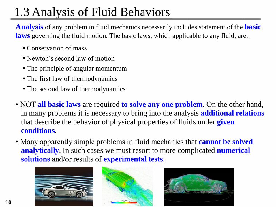
• The viscosity depends on the particular fluid,

and for a particular fluid the viscosity is also

dependent on temperature.

• The gradient of the straight line corresponds

to the dynamic viscosity of the fluid.

• Fluids for which the shearing stress is

linearly related to the rate of shearing strain

(also referred to as rate of angular deformation)

are designated as Newtonian fluids.

• Most common fluids such as water, air, and

gasoline are Newtonian fluid under normal

conditions.

Non-Newtonian Fluids

• Fluids for which the shearing stress is not

linearly related to the rate of shearing strain are

designated as non-Newtonian fluids.

19

1.6 Viscosity

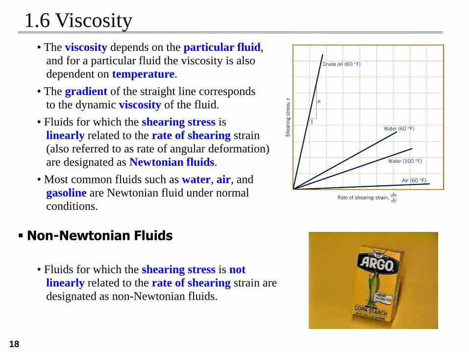
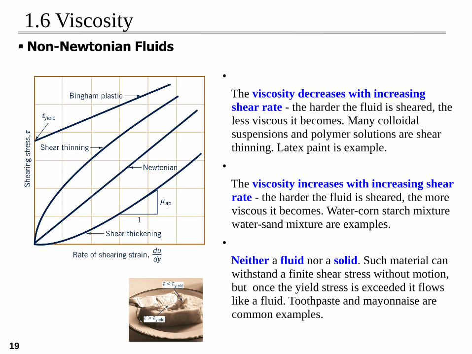
Non-Newtonian Fluids

•

The viscosity decreases with increasing

shear rate - the harder the fluid is sheared, the

less viscous it becomes. Many colloidal

suspensions and polymer solutions are shear

thinning. Latex paint is example.

•

The viscosity increases with increasing shear

rate - the harder the fluid is sheared, the more

viscous it becomes. Water-corn starch mixture

water-sand mixture are examples.

•

Neither a fluid nor a solid. Such material can

withstand a finite shear stress without motion,

but once the yield stress is exceeded it flows

like a fluid. Toothpaste and mayonnaise are

common examples.

20

1.6 Viscosity Temperature Dependence

• For liquid, the viscosity decreases with an increase in temperature.

• For gases, an increase in temperature causes an increase in viscosity.

Why? molecular structure.

The liquid molecules are closely spaced, with strong cohesive

forces between molecules, and the resistance to relative motion between adjacent layers is related to these intermolecular force.

As the temperature increases, these cohesive force are

reduced with a corresponding reduction in resistance to motion.

Since viscosity is an index of this resistance, it follows that viscosity

is reduced by an increase in temperature.

Andrade’s equation μ = DeB/T (D and B are constant)

In gases, the molecules are widely spaced and intermolecular

force negligible.

The resistance to relative motion mainly arises due to the exchange

of momentum of gas molecules between adjacent layers.

As the temperature increases, the random molecular activity

increases with a corresponding increase in viscosity.

Sutherland equation μ = CT3/2/(T+S) (C and S are constant)

21

1.6 Viscosity Kinematic Viscosity (동점성계수)

• Defining kinematic viscosity ν = μ/ρ.

• It is usually denoted by the Greek letter nu (ν).

• Since units for μ and ρ are N∙s/m2 and kg/m3, unit of kinematic viscosity is m2/s.

For example, water at 20 °C has a viscosity of 1.002 mPa·s (10-3 Pa·s).

The cgs(Centimetre–gram–second system of units) physical unit for dynamic viscosity is the poise (P),

named after Jean Poiseuille.

1 P = 1 g∙cm-1∙s-1 = 0.1 kg∙m-1∙s-1

It is more commonly expressed, particularly in ASTM standards, as centipoise (cP).

A centipoise (cP) is one one-hundredth of a poise, and one millipascal-second (mPa·s) in SI units.

(1 cP = 10−2 P = 10−3 Pa·s = 1 mPa·s)

N = [kg∙m/s2]

Physical Unit of Viscosity

μ = (N·s)/m2 = (Pa·s)= (N/m2)·s

= ((kg∙m/s2)·s)/m2= kg/(m·s)

∴ 1 Pa·s = 10 P

22

1.7 Compressibility of Fluids Bulk Modulus (체적계수)

• Liquids are usually considered to be incompressible,

whereas gases are generally considered compressible.

• A property, bulk modulus Ev, is used to characterize compressibility of fluid.

• Measure of how pressure compresses the volume/density.

• Units of the bulk modulus are N/m2 (Pa).

• Large values of the bulk modulus indicate incompressibility.

• Incompressibility indicates large pressures are needed to compress the volume slightly

• It takes 3120 psi to compress water 1% at atmospheric pressure and 15.5°C.

• Most liquids are incompressible for most practical engineering problems.

dρ

dp

V/Vd

dpEυ

p is pressure, V = volume and ρ is the density.

23

1.7 Compressibility of Fluids Compression of Gases

RTp Ideal Gas Law:

• p is pressure, ρ is the density, R is the gas constant, and T is Temperature

constantρ

p

Isothermal Process (constant temperature):

pE

Isentropic Process (frictionless, no heat exchange):

constantkρ

p kpE

k is the ratio of specific heats, Cp (constant pressure) to Cv (constant volume),

R = Cp – Cv.

• If we consider air under at the same conditions as water, we can show that air is

15,000 times more compressible than water.

• However, many engineering applications allow air to be considered incompressible.

Cdρ

dpρp C

dρ

dpEυ C

kρp C1C kρk

dρ

dp 1C k

υ kE

24

1.7 Compressibility of Fluids• When a gas undergoes a reversible process, the

process frequently takes place in such a manner that

a plot of log P versus log V is a straight.

• A process PVn is a constant called a polytropic

process.

nVd

Pd

ln

lnd ln P + nd ln V = 0

Polytropic index Relation Effects

n = 0 PV0=P Isobaric process (constant pressure)

n = 1 PV=mRT Isothermal process (constant temperature)

n = ∞ PV∞ Equivalent to an isochoric process (constant volume)

n = k (CP/CV ) PVk Isentropic process (adiabatic and reversible).

25

1.7 Compressibility of Fluids Speed of Sound

• A consequence of the compressibility of fluids is that small disturbances introduced at

a point propagate at a finite velocity. Pressure disturbances in the fluid propagate as

sound, and their velocity is known as the speed of sound or the acoustic velocity, c.

ordρ

dpc

ρ

Ec v

Isentropic Process (frictionless, no heat exchange because):

kpc

Ideal Gas and Isentropic Process:

kRTc

1C kρkdρ

dpkρp Cρ

ρk

k

C

26

• Evaporation occurs in a fluid when liquid molecules at the surface have sufficient

momentum to overcome the intermolecular cohesive forces and escape to the

atmosphere.

• Vapor Pressure (증기압) is that pressure exerted on the fluid by the vapor in a

closed saturated system where the number of molecules entering the liquid are the

same as those escaping. Vapor pressure depends on temperature and type of fluid.

• Boiling occurs when the absolute pressure in the fluid reaches the vapor pressure.

Boiling occurs at approximately 100 °C, but it is not only a function of temperature,but also of pressure. For example, in Colorado Spring (altitude of 1,840m), water boils

at temperatures less than 100 °C.

1.8 Vapor Pressure Evaporation and Boiling

Cavitation is a form of

Boiling due to low pressure

locally in a flow.

27

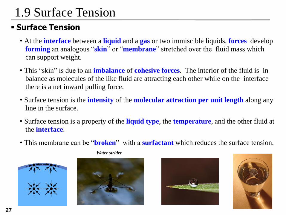
1.9 Surface Tension Surface Tension

• At the interface between a liquid and a gas or two immiscible liquids, forces develop

forming an analogous “skin” or “membrane” stretched over the fluid mass which

can support weight.

• This “skin” is due to an imbalance of cohesive forces. The interior of the fluid is inbalance as molecules of the like fluid are attracting each other while on the interface

there is a net inward pulling force.

• Surface tension is the intensity of the molecular attraction per unit length along any

line in the surface.

• Surface tension is a property of the liquid type, the temperature, and the other fluid atthe interface.

• This membrane can be “broken” with a surfactant which reduces the surface tension.

Water strider

28

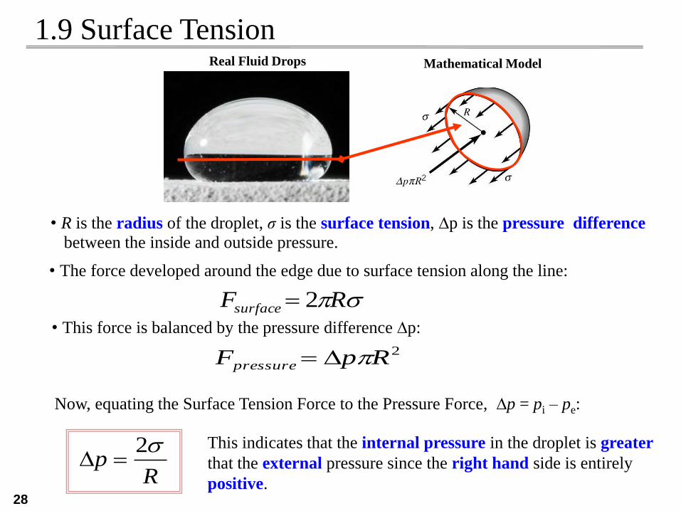
1.9 Surface TensionReal Fluid Drops Mathematical Model

• R is the radius of the droplet, σ is the surface tension, ∆p is the pressure difference

between the inside and outside pressure.

• The force developed around the edge due to surface tension along the line:

• This force is balanced by the pressure difference ∆p:

RFsurface 2

2RpFpressure

Now, equating the Surface Tension Force to the Pressure Force, ∆p = pi – pe:

Rp

2

This indicates that the internal pressure in the droplet is greater

that the external pressure since the right hand side is entirely

positive.

29

1.9 Surface Tension Capillary Action

• Capillary action in small tubes which involve a liquid-gas-solid interface is caused

by surface tension. The fluid is either drawn up the tube or pushed down.

“Wetted” “Non-Wetted”

Adhesion

CohesionAdhesion

Cohesion

• h is the height, R is the radius of the tube, θ is the angle of contact.

• The weight of the fluid is balanced with the vertical force caused by surface tension.

30

1.9 Surface Tension

Equating the two and solving for h:

• For clean glass in contact with water, θ 0°, and thus as R decreases, h increases,giving a higher rise.

• For a clean glass in contact with Mercury, θ 130°, and thus h is negative or there isa push down of the fluid.

31

1.9 Surface TensionTable 1.3 Approximate Physical Properties of Some Common Liquids

Table 1.4 Approximate Physical Properties of Some Common Gases