Chapter 1 – Probability Theory...Chapter 1 for BST 695: Special Topics in Statistical Theory, Kui...

Chapter 1 for BST 695: Special Topics in Statistical Theory, Kui Zhang, 2011

1

Chapter 1 – Probability Theory

Chapter 1.1 – Set Theory Definition: A set is a collection of finite or infinite elements where ordering and multiplicity are generally ignored. Definition 1.1.1: The set, S, of all possible outcomes of a particular experiment is called the sample space for the experiment. Example: toss a coin once. What is the sample space? Solution: { , }S H T .

Example: toss a coin 2 times. What is the sample space? Solution: {( , ),( , ),( , ),( , )}S H H H T T H T T (ordered).

Solution: {( , ),( , ),( , )}S H H T H T T (unordered).

Example: roll a dice twice. What is the sample space? Example: roll the dice until 1 appears and record the number of times that the dice has been rolled. What is the sample space? Solution: {1,2,3, }S .


2

Definition: A sample space is countable if its elements can be put into 1-1 corresponding with a subset of integers. Types of the Sample Space: Countable: finite, infinite Uncountable: infinite Definition 1.1.2: An event is any collection of possible outcomes of an experiment, i.e., any subset of S including S itself. Note: An event A is said to occur if the outcome of the experiment is in the set A. Two Relationships defining order and equality: 1. A B x A x B (containment, i.e., A is a subset of B) 2. and A B A B B A (equality) Elementary Set Operations: 1. Union: { : or }A B x x A x B , i.e., set of elements that belong to A or B or both

2. Intersection: { : and }A B x x A x B i.e., set of elements that belong to both A and B

3. Complementation: { : }cA x x A , i.e., set of elements that are not in A.

Definition: An empty set is a set with no elements and is denoted by . Question: What is the complement of the sample space S?


3

Example: If the sample space is the suits of drawing a card at random from a standard deck. Define the outcomes in the following events.

A = {C, D} B = {D, H, S}

Find the following: cA , A B , A B Theorem 1.1.4: For any 3 events, A, B, and C, defined on a sample space S, 1. Commutativity: , A B B A A B B A

2. Associativity: ( ) ( )A B C A B C , ( ) ( )A B C A B C

3. Distributive Laws: ( ) ( ) ( )( ) ( ) ( )

A B C A B A CA B C A B A C

4. DeMorgan’s Laws: ( )c c cA B A B , ( )c c cA B A B

Infinite (countable) union and intersection: Let 1 2, , ,A A be a collection of sets defined on a sample space S. Then

1

{ : for some }i ii

A x S x A i

1

{ : for all }i ii

A x S x A i


4

Example: (0, )S , (0, )( 1,2, )iA i i , then 1

(0, )ii

A

and 1

(0,1)ii

A

.

Uncountable union and intersection: Let be an index set, i.e., a set of elements to be used as indices. Then

{ : for some }a aa

A x S x A a

{ : for all }a aa

A x S x A a

Example: (0, )S , (0, )( (0, ))xA x x , then (0, )

(0, )xx

A

and (0, )

xx

A

.

Definition 1.1.5: Two events A and B are disjoint (or mutually exclusive) if A B . The events 1 2, ,A A are pairwise disjoint (or mutually exclusive) if i jA A for all i j .

Definition 1.1.6: If 1 2, ,A A are pairwise disjoint and 1 iiA S

, then the collection 1 2, ,A A forms a partition

of S .

Verbal Description of Event Set A or B (at least one of A or B) A B A and B A B Not A cA


5

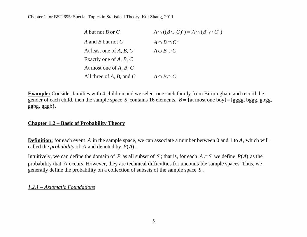
A but not B or C (( ) ) ( )c c cA B C A B C

A and B but not C cA B C At least one of A, B, C A B C Exactly one of A, B, C At most one of A, B, C All three of A, B, and C A B C

Example: Consider families with 4 children and we select one such family from Birmingham and record the gender of each child, then the sample space S contains 16 elements. B {at most one boy}={gggg, bggg, gbgg, ggbg, gggb}. Chapter 1.2 – Basic of Probability Theory Definition: for each event A in the sample space, we can associate a number between 0 and 1 to A , which will called the probability of A and denoted by ( )P A .

Intuitively, we can define the domain of P as all subset of S ; that is, for each A S we define ( )P A as the probability that A occurs. However, they are technical difficulties for uncountable sample spaces. Thus, we generally define the probability on a collection of subsets of the sample space S . 1.2.1 – Axiomatic Foundations


6

Definition 1.2.1: A collection of subsets of S is called a sigma algebra (or Borel field), denoted by , if it satisfies the following three properties: 1. ; (the empty set is an element of ).

2. If A , then cA ; (closed under complementation).

3. If 1 2, ,A A , then 1 iiA

( is closed under countable unions).

This definition implies that if 1 2, ,A A , then 1 iiA

( is closed under countable intersections) (Why?).

Example 1.2.2: If the S is the sample space, then { , }S is an sigma algebra;

{all subsets of , including itself}S S is an sigma algebra; Given A S and A S , then { , , , }cA A S is an sigma algebra. Example 1.2.3: Let { , }S , the real line. Then is chosen to contain all sets of the form [ , ],( , ],( , ), and [ , )a b a b a b a b for all real numbers a and b. Also, from the definition of , it contains all sets that can be formed by taking (possibly countable infinite) unions and intersections of sets of the above varieties. Note: We only consider a sigma algebra that satisfies: (1) it contains [ , ],( , ],( , ), and [ , )a b a b a b a b ; and (2) for any other sigma algebra 1 that contains [ , ],( , ],( , ), and [ , )a b a b a b a b , then 1 . If ( )a a are all sigma algebras containing the above sets, then aa

is such a sigma algebra.

Definition 1.2.4: Given a sample space S and an associated sigma algebra , a probability function is a function P with domain that satisfies 1. ( ) 0P A for all A .


7

2. ( ) 1P S .

3. If 1 2, ,A A are pairwise disjoint, then 11

( ) ( )i iiiP A P A

(known as Axiom of Countable Additivity).

Axiom of Finite Additivity: If A and B are disjoint, then ( ) ( ) ( )P A B P A P B .

Notes: 1) The three conditions in Definition 1.2.4 are known as the Kolmogorov’s axioms of probability named after Andrey Kolmogorov, one of the founders of probability theory. 2) A function P that satisfies these axioms of probability is called a probability function. 3) The axiom of countable additivity implies the axiom of finite additivity, but the axiom of finite additivity does not imply the axiom of countable additivity. Example 1.2.5: Tossing a fair (or balanced) coin. What is the sample space, S ? How would we assign probabilities to each outcome of this experiment to assure that we have a valid probability function? Theorem 1.2.6: Let 1{ , , }nS s s be a finite set. Let be any sigma algebra of subsets of S . Let 1, , np p be nonnegative numbers that sum to 1. For any A , define ( )P A by

:( )

iii s A

P A p

. Then P is a probability

function on . This remains true if 1 2{ , , }S s s is a countable set.

Example: toss a fair coin 2 times. What is the sample space S ? How to define the probability on S . Solution: {( , ),( , ),( , ),( , )}S H H H T T H T T (ordered)

(( , )) (( , )) (( , )) (( , )) 0.25P H H P H T P T H P T T .


8

Solution: {( , ),( , ),( , )}S H H T H T T (unordered)

(( , )) (( , )) 0.25, (( , )) 0.50P H H P T T P H T .

Example: Consider repeated tossing a coin with ( ) (0 1)P H p p . The experiments terminates the first time a head shows up. If we record the number of times that the coin has been tossed, then {1,2, ,}S , we can define

1({ }) (1 )kP k p p .

Theorem 1.2.6: Let 1{ , , }nS s s be a finite set. Let be any sigma algebra of subsets of S . Let 1, , np p be nonnegative numbers that sum to 1. For any A , define ( )P A by

:( )

iii s A

P A p

. Then P is a probability

function on . This remains true if 1 2{ , , }S s s is a countable set.

Calculating the probability of an Event: The following steps can be used to find a probability of an event from a countable sample space:

1. Define the experiment, determine the possible outcomes, and construct the sample space S . 2. Define probability function P on S .

3. Define the event of interest A , and calculate its probability using: :

( )i

ii s AP A p

.

Example 1.2.7: Example: A balance coin is tossed three times. Calculate the probability that exactly two of the three tosses results in heads.


9

Solution: ( ) 3/8P A .

1.2.2 The Calculus of Probability Theorem 1.2.8: If P is a probability function and A is any set in , then 1. ( ) 0P ;

2. ( ) 1P A ;

3. ( ) 1 ( )cP A P A .

Example: Suppose a pair of fair dice is rolled. What is the probability that the sum of face values is at least 4? Solution:

( ) 33/36 11/12P A .

{( , ) :1 6,1 6}S i j i j .

{( , ) : ( , ) ,and 3} {(1,1), (1,2),(2,1)}cB A i j i j S i j .

Theorem 1.2.9: If P is a probability function and A is any set in , then

1. ( ) ( ) ( )cP B A P B P A B ;

2. ( ) ( ) ( ) ( )P A B P A P B P A B ;

3. If A B , then ( ) ( )P A P B .


10

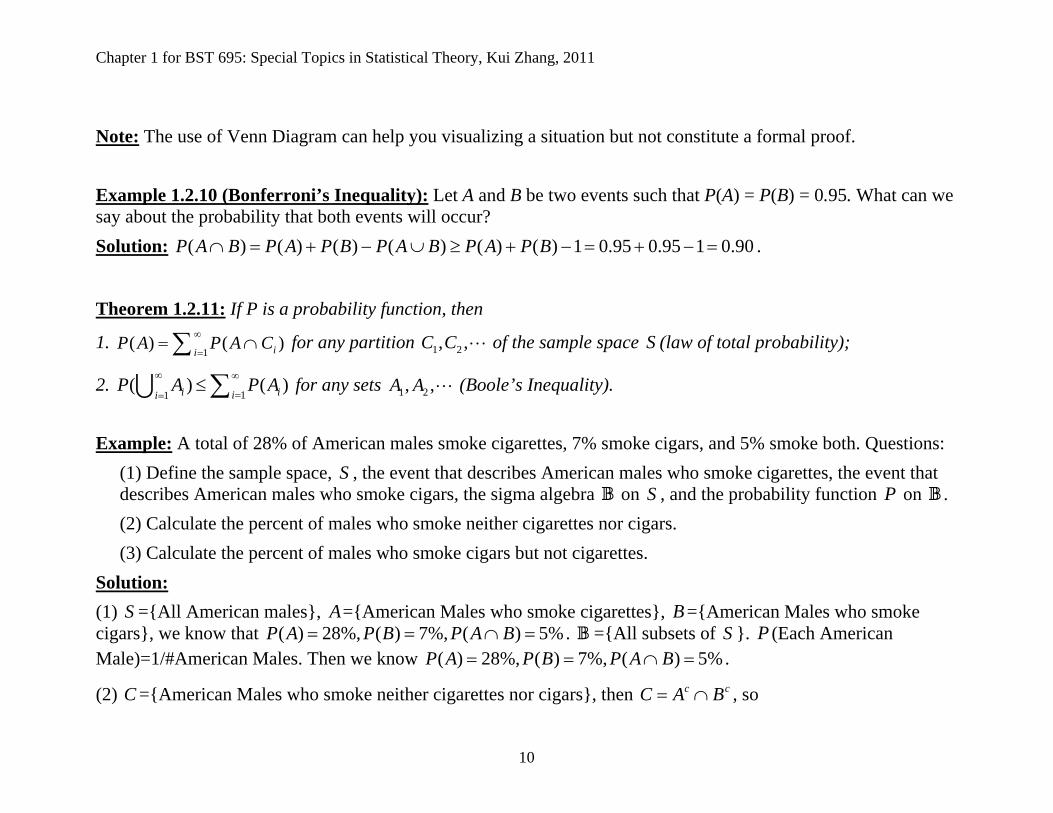
Note: The use of Venn Diagram can help you visualizing a situation but not constitute a formal proof. Example 1.2.10 (Bonferroni’s Inequality): Let A and B be two events such that P(A) = P(B) = 0.95. What can we say about the probability that both events will occur? Solution: ( ) ( ) ( ) ( ) ( ) ( ) 1 0.95 0.95 1 0.90P A B P A P B P A B P A P B .

Theorem 1.2.11: If P is a probability function, then

1. 1

( ) ( )iiP A P A C

for any partition 1 2, ,C C of the sample space S (law of total probability);

2. 11

( ) ( )i iiiP A P A

for any sets 1 2, ,A A (Boole’s Inequality).

Example: A total of 28% of American males smoke cigarettes, 7% smoke cigars, and 5% smoke both. Questions:

(1) Define the sample space, S , the event that describes American males who smoke cigarettes, the event that describes American males who smoke cigars, the sigma algebra on S , and the probability function P on . (2) Calculate the percent of males who smoke neither cigarettes nor cigars. (3) Calculate the percent of males who smoke cigars but not cigarettes.

Solution: (1) S ={All American males}, A={American Males who smoke cigarettes}, B ={American Males who smoke cigars}, we know that ( ) 28%, ( ) 7%, ( ) 5%P A P B P A B . ={All subsets of S }. P (Each American Male)=1/#American Males. Then we know ( ) 28%, ( ) 7%, ( ) 5%P A P B P A B .

(2) C ={American Males who smoke neither cigarettes nor cigars}, then c cC A B , so


11

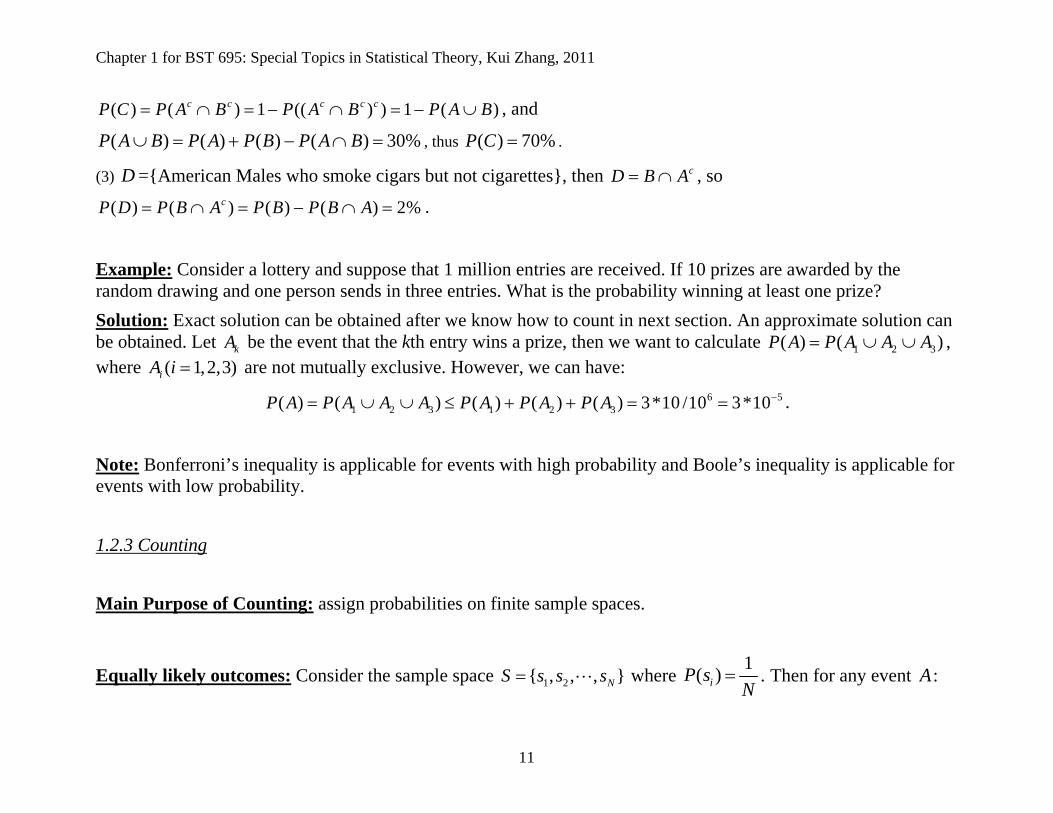
( ) ( ) 1 (( ) ) 1 ( )c c c c cP C P A B P A B P A B , and

( ) ( ) ( ) ( ) 30%P A B P A P B P A B , thus ( ) 70%P C .

(3) D ={American Males who smoke cigars but not cigarettes}, then cD B A , so

( ) ( ) ( ) ( ) 2%cP D P B A P B P B A .

Example: Consider a lottery and suppose that 1 million entries are received. If 10 prizes are awarded by the random drawing and one person sends in three entries. What is the probability winning at least one prize? Solution: Exact solution can be obtained after we know how to count in next section. An approximate solution can be obtained. Let kA be the event that the kth entry wins a prize, then we want to calculate 1 2 3( ) ( )P A P A A A , where ( 1,2,3)iA i are not mutually exclusive. However, we can have:

6 51 2 3 1 2 3( ) ( ) ( ) ( ) ( ) 3*10 /10 3*10P A P A A A P A P A P A .

Note: Bonferroni’s inequality is applicable for events with high probability and Boole’s inequality is applicable for events with low probability. 1.2.3 Counting Main Purpose of Counting: assign probabilities on finite sample spaces.

Equally likely outcomes: Consider the sample space 1 2{ , , , }NS s s s where 1( )iP sN

. Then for any event A :


12

1 # of elements in ( ) ({ ))# of elements in Si i

is A s A

AP A P sN

.

Theorem 1.2.14: If a job consists of k separate tasks, the i th of which can be done in in ways, 1,2, ,i k , then the entire job can be done in 1 2 kn n n ways.

Example (number of license plates): Suppose a license plate consists of three letters of alphabet followed by two integers from 0 to 9. What is the total number of plates possible? Solution: 26*26*26*10*10=1,757,600. Example 1.2.15: If you can pick up 6 numbers from 1 to 44 in a lottery game, how many ways can you choose in the first two steps? If the order does not matter, how many combinations of two numbers can you get in the first two steps? Solution: If you can not choose the same number twice, then we have 44 43 1892 ways. But if you are allowed to choose the same number twice, then we have 44 44 1936 ways. If you can not choose the same number twice and the order does not matter, then we have 44 43/ 2 946 combinations. If you are allowed to choose the same number twice and the order does not matter, the we have 44 43/ 2 44 990 . Actually, the aforementioned example highlights two important factors on methods of counting: replacement and order, we can have four situations:

Possible methods for counting

Without Replacement

With Replacement


13

Ordered Unordered

Definition 1.2.16: For a positive integer n , !n (read as n factorial) is the product of all the positive integers less than or equal to n , i.e. ! ( 1) 2 1n n n . Furthermore, we define 0! 1 .

Examples 1.2.15 (continue): If you can pick up 6 numbers from 1 to 44 in a lottery game, how many ways do you have? ordered, without replacement:

44!44 43 42 41 40 3938!

ordered, with replacement:

644 44 44 44 44 44 44 unordered, without replacement

44 43 42 41 40 39 44!6 5 4 3 2 1 6!38!

Definition 1.2.17: For nonnegative integers n and r , where n r , we define the symbol


14

nr

, read n choose r , as !!( )!

n nr r n r

(binomial coefficients).

unordered, with replacement:

49!6!43!

In summary, we have the following table:

Number of possible arrangements of size r from n subjects

Without

Replacement ( r n )

With Replacement

Ordered Unordered

!( )!

nn r

rn

nr

1n r

r

1.2.4 Enumerating Outcomes

Equally likely outcomes: Consider the sample space 1 2{ , , , }NS s s s where 1( )iP sN

. Then for any event A:


15

1 # of elements in ( ) ({ ))# of elements in Si i

is A s A

AP A P sN

.

Example 1.2.18: In a poker game (draw 5 cards without replacement), find the probability of getting

(i) four aces (ii) four of a kind (iii) exactly one pair

Example: Suppose there are ( 365)n n students in our class, then what is the probability that at least two students have the same birthday (ignoring the year of their birth and considering there are only 365 days in a year).

Solution: 365

1 ( !) /365nP nn

.

Define the event A={at least two students have the same birthday}.

then cA ={All students have the different birthday}.

# of elements in the sample space S = 365n .

# of elements in the event cA = 365365! !

(365 )!n

nn

Table: n 10 20 30 40 50 ( )P A 0.12 0.41 0.71 0.89 0.97


16

Example: Consider a lottery and suppose that 1 million entries are received. If 10 prizes are awarded by the random drawing and one person sends in three entries. What is the probability winning at least one prize? What is the probability winning exact two prizes?

Solution: Let cA be the event that none of three entries wins the prize. The sample space S contains 1000000

10

elements and the event cA contains 999997

10

elements. Thus:

-5999997 1000000( ) 1 ( ) 1 / 2.999973*10

10 10cP A P A

.

Recall the previous solution: Let kA be the event that the kth entry wins a prize, then we want to calculate 1 2 3( ) ( )P A P A A A , where ( 1,2,3)iA i are not mutually exclusive. However, we can have:

6 51 2 3 1 2 3( ) ( ) ( ) ( ) ( ) 3*10 /10 3*10P A P A A A P A P A P A .

Question: why are ( 1,2,3)iA i not mutually exclusive?

Let B be the event that two of three entries win the prize, then B contains 3 9999972 8

elements.

Example 1.2.19 (Sampling with replacement): Consider sampling items from 3n objects, with replacement. The outcomes in the ordered and unordered sample spaces are these:

Unordered {1,1} {2,2} {3,3} {1,2} {1,3} {2,3}


17

Ordered (1,1) (2,2) (3,3) (1,2),(2,1) (1,3),(3,1) (2,3),(3,2)Probability 1/9 1/9 1/9 2/9 2/9 2/9

Example (Sampling without replacement): Consider sampling 2r items from 3n objects, without replacement. The outcomes in the ordered and unordered sample spaces are these:

Unordered {1,2} {1,3} {2,3} Ordered (1,2),(2,1) (1,3),(3,1) (2,3),(3,2)

Probability 1/3 1/3 1/3 Note:

1. To calculate the right probability, you must use the right sample space to count the number of elements in the event and the sample space. The right sample space means that all elements in the sample space have the same probabilities.

2. For sampling without replacement, if we want to calculate the probability of an event that does not depend on the order, we can use either the ordered space or the unordered space.

3. For the sampling with replacement, if we want to calculate the probability of an event that does not depend on the order, we must use the ordered space. This is corresponds to the common interpretation of “sampling with replacement”. For example 1.2.19, that means one of three objects is chosen, each with probability of 1/3, the object is noted and replaced; three objects are mixed and again one of them is chosen, each with probability of 1/3. Thus, six unordered outcomes do not have the equal probability, but nine ordered outcomes have the equal probability under this sampling scheme.

Example 1.2.18: In a poker game (draw 5 cards without replacement), find the probability of getting four of a kind.


18

Solution: Ordered: 52

# 52!/ 47!,# 13* 48*5!, ( ) # /# 13* 48/5

S A P A A S

.

Unordered: 52 52

# ,# 13* 48, ( ) # /# 13* 48/5 5

S A P A A S

.

Review for the previous lecture Theorem: How to calculate probabilities of events (1.2.8, 1.2.9, 1.2.11)

Definition: !n , nr

.

Theorem: How to count. Number of possible arrangements of size r from n subjects

Without

Replacement ( r n )

With Replacement

Ordered !

( )!n

n r rn

Unordered nr

1n r

r

Example: Enumerating Outcomes


19

1.3 Conditional Probability and Independence Example 1.3.1: What is the probability having four aces when 4 cards are drawn from a poker game?

Solution 1 (Counting Rules): 52

1/4

(unordered space).

Solution 2 (Conditioning rules): 4 /52 3/51 2/50 1/ 49 . Definition 1.3.2: If A and B are events in S , and ( ) 0P B , then the conditional probability of A given B , written as ( | )P A B , is ( | ) ( ) / ( )P A B P A B P B . Specifically, if A and B are disjoint, then

( | ) ( | ) 0P A B P B A .

Example 1.3.3: P (4 aces in four cards| i aces in i cards)= P (4 aces in four cards)/ P ( i aces in i cards), which

equals to

521/

44 52

/i i

.

Remark:

1. We require ( ) 0P B for the calculation. We will defer the discussion of this until Chapter 4.


20

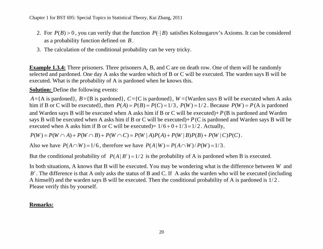
2. For ( ) 0P B , you can verify that the function ( | )P B satisfies Kolmogarov’s Axioms. It can be considered as a probability function defined on B .

3. The calculation of the conditional probability can be very tricky. Example 1.3.4: Three prisoners. Three prisoners A, B, and C are on death row. One of them will be randomly selected and pardoned. One day A asks the warden which of B or C will be executed. The warden says B will be executed. What is the probability of A is pardoned when he knows this. Solution: Define the following events: A={A is pardoned}, B ={B is pardoned}, C ={C is pardoned}, W ={Warden says B will be executed when A asks him if B or C will be executed}, then ( ) ( ) ( ) 1/3P A P B P C , ( ) 1/ 2P W . Because ( )P W P (A is pardoned and Warden says B will be executed when A asks him if B or C will be executed)+ P (B is pardoned and Warden says B will be executed when A asks him if B or C will be executed)+ P (C is pardoned and Warden says B will be executed when A asks him if B or C will be executed)= 1/ 6 0 1/3 1/ 2 . Actually,

( ) ( ) ( ) ( ) ( | ) ( ) ( | ) ( ) ( | ) ( )P W P W A P W B P W C P W A P A P W B P B P W C P C .

Also we have ( ) 1/ 6P A W , therefore we have ( | ) ( ) / ( ) 1/3P A W P A W P W .

But the conditional probability of ( | ) 1/ 2cP A B is the probability of A is pardoned when B is executed.

In both situations, A knows that B will be executed. You may be wondering what is the difference between W and cB . The difference is that A only asks the status of B and C. If A asks the warden who will be executed (including

A himself) and the warden says B will be executed. Then the conditional probability of A is pardoned is 1/ 2 . Please verify this by yourself. Remarks:


21

1. ( | ) ( | ) ( ) /( ( ) ( ) ( ))( | ) ( ) /( ( | ) ( ) ( | ) ( ) ( | ) ( )).

P A W P W A P A P W A P W B P W CP W A P A P W A P A P W B P B P W C P C

2. ( ) ( | ) ( ) ( | ) ( )P A B P A B P B P B A P A .

3. 1 1

( ) ( ) ( | ) ( )i i ii iP B P B A P B A P A

Example (Distribution of Students by Sex and Declared Major): The distribution of 1237 students at community college by sex and declared major is given below

Sex Arts and Sciences

(A) Business

(B) Music

(C) Total

Male (M) 127 383 40 550 Female (F) 380 242 65 687

Total 507 625 105 1237 If a business major is randomly selected from this college, what is the probability that the student is a female? Solution: ( | ) ( ) / ( ) 242/ 625P F B P F B P B .

Theorem 1.3.5 (Bayes’ Rule) Let 1 2, ,A A be a partition of the sample space and let B be any set. Then, for each

1,2,i ,

1 1

( ) ( | ) ( ) ( | ) ( )( | )( ) ( ) ( | ) ( )i i i i i

ik k kk k

P A B P B A P A P B A P AP A BP B P B A P B A P A


22

The meaning of Bayes’ Rule: 1 2, ,A A can be considered as the reasons that results the event B . So ( | )iP B A is generally called as the prior probability and determined by previous experiments. If the event B occurred, this formula can help us to find which reason results the event B . ( | )iP A B is generally called the “posterior probability”. Example 1.3.6: Morse Codes. Example (Making a Sale): Consider a local manufacture of mattress who consistently runs a sales campaign in the local media. In order to evaluate the effectiveness of the campaign, the manufacture keeps a record of whether or not a customer has been the advertisement and whether or not the customer makers a purchase. From this data, we can estimate the probability that a randomly selected customer will make a purchase. Solution: Let S be the event that a customer make a purchase and A be the event that a customer has been the advertisement, then ( ) ( ) ( ) ( | ) ( ) ( | ) ( )c c cP S P S A P S A P S A P A P S A P A . If we can estimate ( ) 0.6P A ,

( | ) 0.7P S A , and ( | )cP S A =0.2, then ( ) 0.50P S .

Example (Medical Diagnosis): In medical diagnosis a doctor observed that a patient has one symptoms A and is faced with the problem of deciding which of the several possible diseases 1 2( , , , )nD D D . Suppose that ( )iP D and

( | )iP A D can be estimated from the historical data. We additionally assume that the diseases never occur in the

same person, then 1

( | ) ( ) ( | ) / ( ) ( | )ni i i j jj

P D A P D P A D P D P A D

. If ( | )kP D A has the highest probability and no

further information, the patient should be treated for disease kD .

In particular, let 1( ) 0.4P D , 2( ) 0.25P D , 3( ) 0.35P D , and 1( | ) 0.8P A D , 2( | ) 0.6P A D , 3( | ) 0.9P A D , then 3

1( ) ( | ) ( ) 0.785i ii

P A P A D P D

, 1( | ) 0.41P D A , 2( | ) 0.19P D A , 3( | ) 0.40P D A .


23

Definition 1.3.7: Two events, A and B are statistically independent if ( ) ( ) ( )P A B P A P B . Equivalently, A and B are statistically independent if ( | ) ( ) where ( ) 0P A B P A P B or ( | ) ( )P B A P B where ( ) 0P A .

Theorem 1.3.9: If A and B are independent events, then the following pairs are also independent:

(a) A and cB ; (b) cA and B ; (c) cA and cB . Example (Sampling with replacement and without replacement): A lot contains 1000 items of which five are defective. Two items are randomly drawn as follows. The first item drawn is tested and replaced in the lot and then the second item is drawn and tested. Let iA be the event that ith item drawn is defective. Then 1A and 2A are independent events.

Solution: 5( )

1000iP A , 1 2 1 2( ) 25/(1000*1000) ( ) ( )P A A P A P A .

If the first item is not replaced in the lot, then 1A and 2A are not independent events:

5( )1000iP A (why?), 1 2 1 2 1( ) 5* 4 /(1000*999) ( ) ( | ) (5/1000)(4 /1000)P A A P A P A A .

Definition 1.3.12: A collection of events 1 2, ,A A are mutually independent if for any subcollection

1 2, , ,ki i iA A A ,

we have

11

( ) ( )j j

k k

i ijj

P A P A

.


24

Remark: If a collection of events 1 2, ,A A are mutually independent, then all the pairs of them are independent. However, even all of pairs are independent; they may not be mutually independent. Remark: If a collection of events 1 2, ,A A are mutually independent, then 1 2, ,B B are mutually independent for

i iB A or ( 1,2, )ci iB A i .

Question: If a collection of events 1 2, ,A A are mutually exclusive, then are 1 2, ,B B mutually exclusive for

i iB A or ( 1,2, )ci iB A i ?

Notes:

1. If 1 2, ,A A are mutually independent, then 11

( ) ( )i iiiP A P A

.

2. 1 2, ,A A are mutually exclusive, then 11

( ) ( )i iiiP A P A

.

3. DeMorgan’s laws relate the operation of union and intersection. For example, if 1 2, ,A A are mutually

independent, then 1 11 1 1

( ) 1 (( ) ) 1 ( ) 1 ( ) 1 (1 ( ))c c ci i i i ii ii i i

P A P A P A P A P A

.

Examples: If a collection of events 1 2, ,A A are mutually independent, ( )i iP A p ( 1, ,i n ), then calculate the probability of the following events:

(1) 1

n cii

B A

(none of iA occurs): 1

( ) (1 )nii

P B p

.

(2) 1

nii

C A

(at least one of iA occurs): 1

( ) 1 (1 )nii

P C p

.


25

(3)1( ( ))n c

i ji j iD A A

(exactly one iA occurs):

1( ) ( (1 ))n

i ji j iP D p p

.

Example: A large machine consists of 50 components. Past experience has shown that a particular component has a probability of 0.1% to fail. Suppose that the performance of one component will not affect another. The equipment will work if no more than one component fails. What is the probability that the machine will work? Solution: Define iA {the i th component fails}, then ( ) 0.1%iP A and ( 1, ,50)iA i are mutually independent. Define D ={the equipment will work} ={exactly one component fails }{none of component fails}, therefore,

50 4950( ) (1 0.1%) 0.1% *(1 0.1%) 99.88%

1P D

.

We can get ( ) 97.38%P D and ( ) 91.08%P D if ( ) 0.5%iP A and ( ) 1%iP A , respectively.

1.4 Random Variables Example: If we decide to ask 50 people whether they agree or disagree with a certain issue. If we record “1” for the agree and “0” for the disagree. Then we have a sample space with the size of 502 , each an ordered string of 1s and 0s of length 50. Actually, we may be only interested in the number of people who agree (or disagree) out of 50. In this situation, we can define X =number of 1s recorded out of 50. Note now that the sample space X is the set of integers {0,1,2, ,50} , which is easier to be dealt with.

Definition 1.4.1: A random variable is a function from a sample space S into the real numbers.


26

Definition and Theorem: Suppose we have a sample space 1 2{ , , , }nS s s s with a probability function P and we define random variable X with range 1{ , , }mx x , then we can define a function XP on in the following way: ( ) ({ : ( ) })X i j j iP X x P s S X s x . Then XP is a probability function defined on the sample space . We call it as the induced probability function on . We can simply write ( )X iP X x as ( )iP X x . This definition can be extended to countable (infinite) sample spaces (but not to uncountable sample spaces). To generalize this definition, for any set A where is appropriate sigma algebra defined on (in the general case, is derived from the original sigma algebra defined on the sample space S ), we can define:

( ) ({ : ( ) })XP X A P s S X s A .

Notation: A random variable will be denoted by uppercase letter, say X, and the realized values (or its range) will be denoted by the corresponding lower case letters, x. Example: Roll two fair dice, X =sum of face numbers Solution:

s (1,1)(1,2)(2,1)

(1,3)(2,2)(3,3)

(1,4)(2,3)(3,2)(4,1)

(1,5)(2,4)(3,3)(4,2)(5,1)

(1,6)(2,5)(3,4)(4,3)(5,2)(6,1)

(2,6) (3,5) (4,4) (5,3) (6,2)

(3,6)(4,5)(5,4)(6,3)

(4,6)(5,5)(6,4)

(5,6)(6,5)

(6,6)

( )X s 2 3 4 5 6 7 8 9 10 11 12 ( ( ))P X s 1/36 2/36 3/36 4/36 5/36 6/36 5/36 4/36 3/36 2/36 1/36


27

Example 1.4.3: Toss a fair coin 3 times. Define a random variable and obtain its corresponding distribution. Solution: X =number of heads;

s HHH HHT,HTH,THH TTH, HHT, HTT TTT( )X s 3 2 1 0

( ( ))P X s 1/8 3/8 3/8 1/8

Example 1.4.4 (Distribution of a random variable): If we toss a fair coin n times, and define X number of heads, then what is its corresponding distribution. Solution:

( )P X k P (there are k heads in n coins)= / 2nnk

( 0,1, , )k n .

1.5 Distribution Functions Definition 1.5.1: The cumulative distribution function or cdf of a random variables X , denoted by ( )XF x , is defined by ( ) ( )X XF x P X x , for all x .

Example 1.5.2: Tossing three coins. X =number of heads. Then we have:


28

0 if 01/8 if 0 1

( ) 4/8 if 1 27/8 if 2 31 if 3

X

xx

F x xx

x

Theorem 1.5.3: The function ( )F x is a cdf if and only if the following three conditions hold:

(1) lim ( ) 0x F x and lim ( ) 1x F x .

(2) ( )F x is nondecreasing function of x .

(3) ( )F x is right-continuous; that is, for every number 0x , 0 0lim ( ) ( )x x F x F x .

Proof of necessity: (2) x y , define { : ( ) }A s S X s x and { : ( ) }B s S X s y , then A B , therefore:

( ) ({ : ( ) }) ( ) ( ) ({ : ( ) }) ( )F x P s S X s x P A P B P s S X s y F y

(1) First, ( ) ({ : ( ) })F x P s S X s x , then 0 ( ) 1F x . Define { : 1 ( ) }nA s S n X s n

( , , 1,0,1, , )n , then we have nnS A

, ( ) ( ) ( 1)nP A F n F n , and ( , , )nA n are disjoint.

Therefore, 1 ( ) ( ) ( ( ) ( 1)) lim ( ) lim ( )n n mn nP S P A F n F n F n F m

. Because ( )F x is non

decreasing, we have lim ( ) lim ( )x nF x F n and lim ( ) lim ( )x mF x F m .

(3) To prove ( )F x is right-continuous, we only need to prove for any 1 0nx x x and 0limn nx x , such that 0lim ( ) ( )n nF x F x . It is easy to see


29

1 0 0 1 11

1 1 11

( ) ( ) ({ : ( ) }) ( { : ( ) })

( ( ) ( )) ( ) lim ( )

n nn

n n n nn

F x F x P s x X s x P s x X s x

F x F x F x F x

.

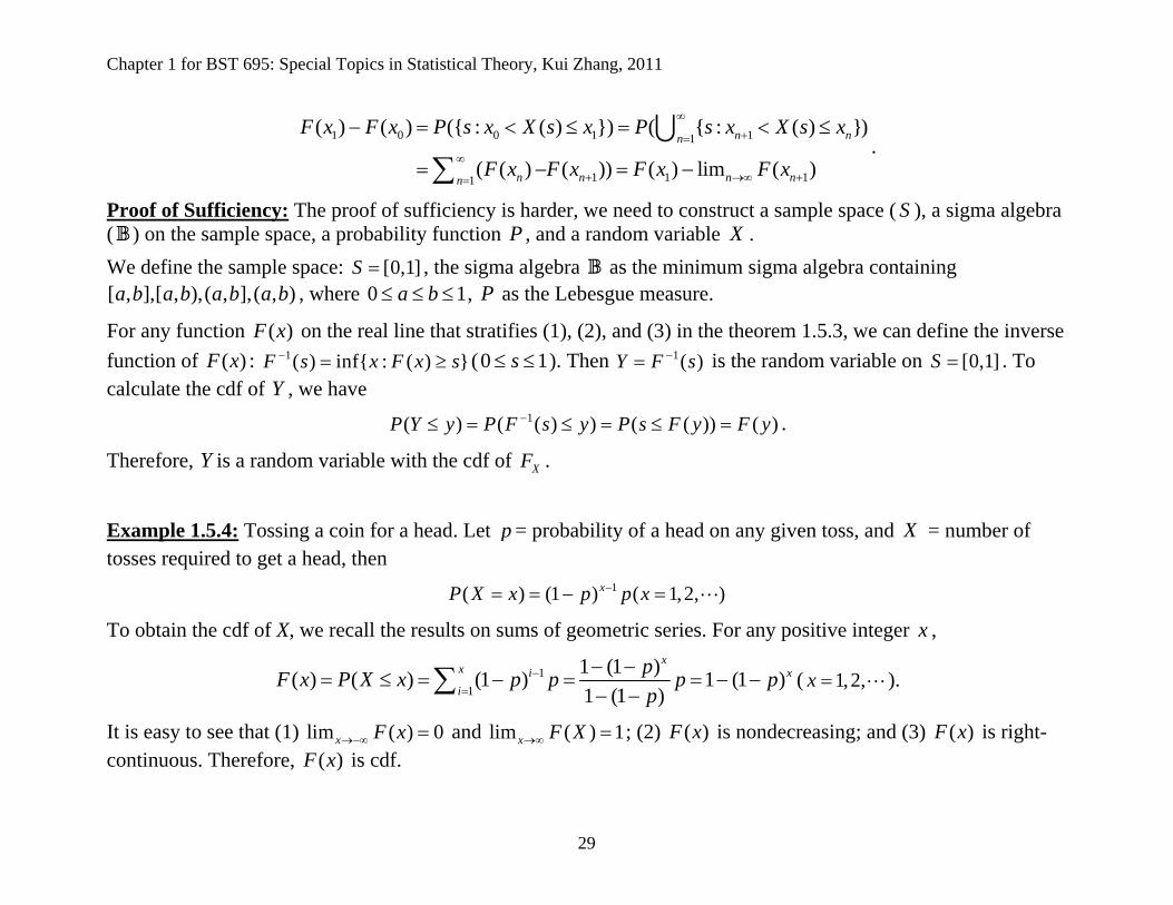
Proof of Sufficiency: The proof of sufficiency is harder, we need to construct a sample space ( S ), a sigma algebra ( ) on the sample space, a probability function P , and a random variable X . We define the sample space: [0,1]S , the sigma algebra as the minimum sigma algebra containing [ , ],[ , ),( , ],( , )a b a b a b a b , where 0 1a b , P as the Lebesgue measure.

For any function ( )F x on the real line that stratifies (1), (2), and (3) in the theorem 1.5.3, we can define the inverse function of ( )F x : 1( ) inf{ : ( ) }F s x F x s (0 1s ). Then 1( )Y F s is the random variable on [0,1]S . To calculate the cdf of Y , we have

1( ) ( ( ) ) ( ( )) ( )P Y y P F s y P s F y F y .

Therefore, Y is a random variable with the cdf of XF .

Example 1.5.4: Tossing a coin for a head. Let p = probability of a head on any given toss, and X = number of tosses required to get a head, then

1( ) (1 ) ( 1,2, )xP X x p p x

To obtain the cdf of X, we recall the results on sums of geometric series. For any positive integer x ,

11

1 (1 )( ) ( ) (1 ) 1 (1 )1 (1 )

xx i xi

pF x P X x p p p pp

( 1,2,x ).

It is easy to see that (1) lim ( ) 0x F x and lim ( ) 1x F X ; (2) ( )F x is nondecreasing; and (3) ( )F x is right-continuous. Therefore, ( )F x is cdf.


30

Example 1.5.5 (Continuous cdf): Show that the following function is a cdf.

1( )1 xF x

e

.

Definition 1.5.7: A random variable X is continuous if ( )F x is a continuous function of x . A random variable X is discrete if ( )F x is a step function of x .

Example 1.5.6: A random variable is neither continuous nor discrete. Consider the following function:

1 if 01( ) for some 0< <1

1 if 01

y

X

y

yeF y

ye

.

Definition 1.5.8: The random variables X and Y are identically distributed if, for every set 1A , ( ) ( )P X A P Y A , where 1 is the smallest sigma algebra containing all the intervals of real numbers of the

form (a, b), [a, b), (a, b], and [a, b]. Theorem 1.5.10: The following two statements are equivalent: 1. The random variables X and Y are identically distributed.


31

2. ( ) ( )X YF x F x for every x .

Example 1.5.9 (Identically distributed random variables): If a fair coin is tossed n times, define the following random variables: X =number of heads observed, and Y =number of tails observed. It is easy to prove that X and Y have the same distribution but they are different. Actually we have ( ) ( )X s Y s n .

1.6 Density and Mass Functions Definition 1.6.1 The probability mass function (pmf) of a discrete random variable X us given by

( ) ( )Xf x P X x for all x .

Note: The pmf gives the point probabilities of a discrete random variable X . Example 1.6.2: From Example 1.5.4, the geometric distribution has pmf given by

1(1 ) for 1,2,( ) ( )

0 otherwise.

x

Xp p x

f x P X x

It follows then that for a b , we have 1( ) ( ) (1 )b b k

Xk a k aP a X b f k p p

.

and in particular, if 1a , then

1( ) ( ) ( ).b

X XkP X b f k F b


32

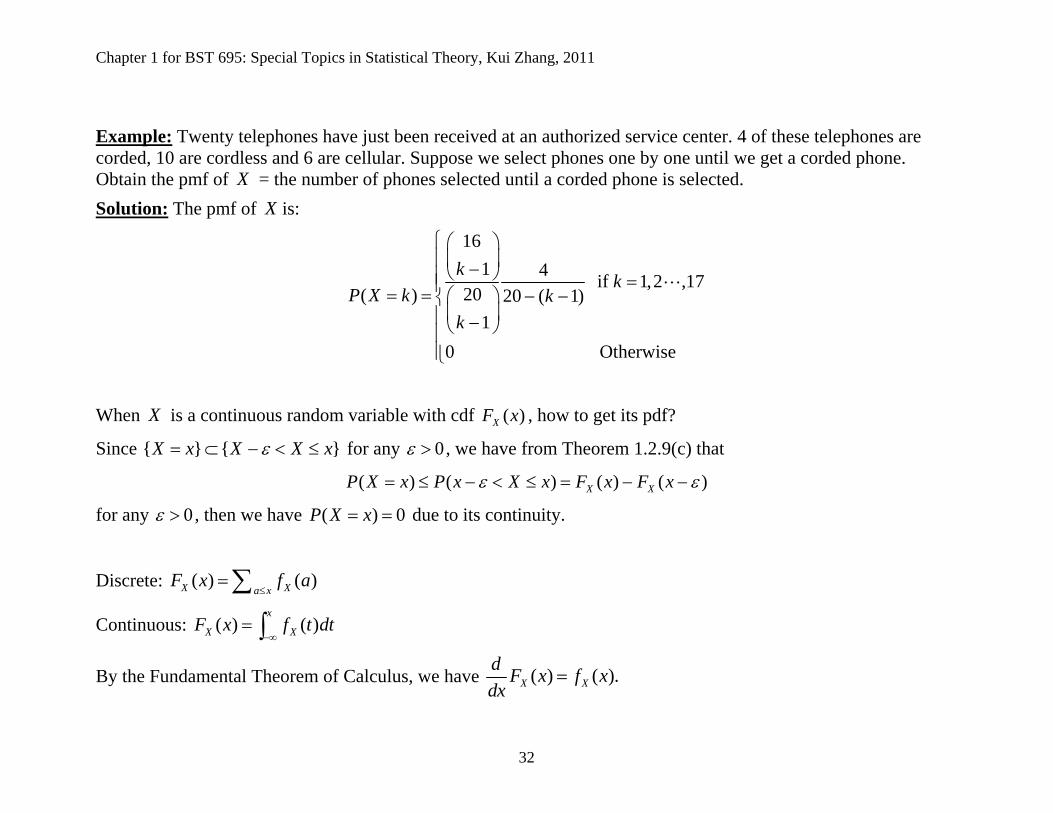
Example: Twenty telephones have just been received at an authorized service center. 4 of these telephones are corded, 10 are cordless and 6 are cellular. Suppose we select phones one by one until we get a corded phone. Obtain the pmf of X = the number of phones selected until a corded phone is selected. Solution: The pmf of X is:

161 4 if 1,2 ,17

20( ) 20 ( 1)1

0 Otherwise

kk

P X k kk

When X is a continuous random variable with cdf ( )XF x , how to get its pdf?

Since { } { }X x X X x for any 0 , we have from Theorem 1.2.9(c) that

( ) ( ) ( ) ( )X XP X x P x X x F x F x

for any 0 , then we have ( ) 0P X x due to its continuity.

Discrete: ( ) ( )X Xa xF x f a

Continuous: ( ) ( )x

X XF x f t dt

By the Fundamental Theorem of Calculus, we have ( ) ( ).X Xd F x f xdx


33

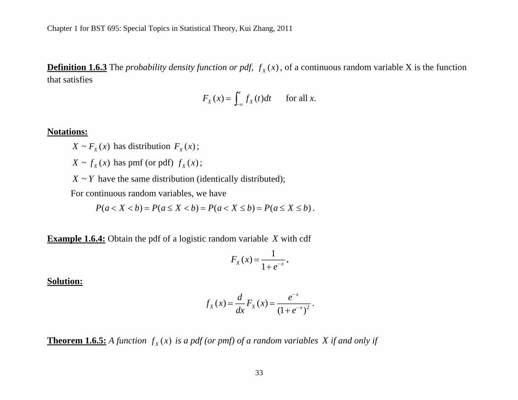
Definition 1.6.3 The probability density function or pdf, ( )Xf x , of a continuous random variable X is the function that satisfies

( ) ( ) for all .x

X XF x f t dt x

Notations:

~ ( )XX F x has distribution ( )XF x ;

~ ( )XX f x has pmf (or pdf) ( )Xf x ;

~X Y have the same distribution (identically distributed); For continuous random variables, we have ( ) ( ) ( ) ( )P a X b P a X b P a X b P a X b .

Example 1.6.4: Obtain the pdf of a logistic random variable X with cdf

1( )1X xF x

e

.

Solution:

2( ) ( )(1 )

x

X X x

d ef x F xdx e

.

Theorem 1.6.5: A function ( )Xf x is a pdf (or pmf) of a random variables X if and only if


34

a. ( ) 0Xf x for all x .

b. ( ) 1Xxf x (pmf) or ( ) 1Xf x dx

(pdf)

Proof. Example: Let X denote the amount of space occupied by an article placed in a 1-ft3 packing container. The pdf of X is:

8(1 ) if 0 1;( )

0 otherwise.Xkx x x

f x

1. Find the value of k that will make this a valid density function. 2. Obtain the cdf of X . Solution:

1. 1 8

0(1 ) /9 /10 1kx x dx k k , thus 90.k

2. 8 9

0 if 0;

( ) if 0 1;9 10

1 if 1 .

X

xkx kxF x x

x

Remarks:

1. We emphasize that the distribution of X is uniquely determined by its cdf or pdf (pmf). So when we ask you to find the distribution of X , it is sufficient to find either cdf or pdf (pmf).


35

2. We note if the sample space S is discrete, then X on S is discrete. if the sample space S contains an interval of ( , ) , then X on S can be discrete, continuous, and mixed.

3. For continuous random variable, cdf and pdf have the following relationships:

( ) ( ) ( )x

X XP X x F x f t dt

and ( ) ( )X Xdf x F xdx

.

4. In practice no real world experiments can yield continuous random variables. The assumption that X is continuous type is a simplifying assumption leading to an idealized description of the model.

5. We emphasize that cdf and pdf (pmf) are defined for all real number x . However, for simplicity, we only concern ( ) 0P X x for discreet random variables and { : ( ) 0}Xx f x for continuous random variables.

Chapter 1 – Probability Theory...Chapter 1 for BST 695: Special Topics in Statistical Theory, Kui...

Documents

Transcript of Chapter 1 – Probability Theory...Chapter 1 for BST 695: Special Topics in Statistical Theory, Kui...