Chaotic analysis of daily and weekly rainfall … 20-6 (web)/paper6.pdfChaotic analysis of daily and...

S. Tamil Selvi and R. Samuel Selvaraj

566

Chaotic analysis of daily and weekly rainfall timeseries over Chennai

S. Tamil Selvi*1 and R. Samuel Selvaraj2

1Research centre, Department of Physics, Bharathiar University, Coimbatore, Tamil Nadu, India2Department of Physics, Presidency College, Chennai, Tamil Nadu, India

*Corresonding Author : [email protected]

ABSTRACTIn this work the reconstruction of phase space and G-P algorithm (correlation dimension) are used to study the chaotic characteristics of daily and weekly rainfall at Chennai, Tamil Nadu. The results show that the daily and weekly rainfall series have a low dimensional chaos. This is also verified using Lyapunov exponent method, which is used to confirm the presence of chaos.The maximum Lyapunov exponent is used to calculate the predictability time. The essential number of parameters in the embedding dimension for the two series were calculated to be 2. The sufficient number of parameters were calculated to be 4 and 6 respectively. The presence of large number of zeros in the high resolution time series may result in underestimation of the dimension, still correlation dimension is the elementary test for the chaos identification. The embedding dimension calculated from the correlation dimension givesthe underlining number of parameters to be used in the forecast model.

Key words: correlation dimension, daily and weekly rainfall, low dimensional chaos, Lyapunov exponent method and embedding dimension.

INTRODUCTION

Time series data, such as rainfall, are very complex to model and study. The difficulty lies in the large range of variability displayed, both in time and space. The variables are mostly inter-related and they are stochastic and unpredictable. Nonlinear dynamics is a rapidly growing field with a new set of tools to analyse such complex processes. Investigation of the presence of low dimensional chaotic behaviour in rainfall dynamics has been of much interest lately. India Meteorological Department (IMD) has been using the power regression and parametric models for long range forecast of monsoon rainfall. These models are used for long range forecast over India, as a whole and for the four clusters of meteorological subdivisions. The statistical models have innate limitations as an alternate technique for the forecast of monsoon rainfall is desirable. Such a model has not been developed so far forecasting techniques for individual states and meteorological subdivisions (Rajeevan, Michaeland and McPhaden, 2004). The Indian rainfall, especially the summer monsoon system has been analysed extensively. The winter monsoon or the northeast monsoon is very less investigated, due its complexity. This paper explores the possible number of variables that may govern the dynamics in the rainfall series during northeast monsoon season over Chennai city.

In any system, if the underlying dynamics is governed by a deterministic equation, the system exhibits a nonlinear chaotic nature which could be random (Kantz, Holger, and Schreiber, 2004).The randomness in most of the natural systems can be attributed to this reason. Initially,most of

the forecast techniques used linear stochastic approach (Harms, Archie and Campbell, 1967; Klemes, 1978; Salas et al., 1981) mainly due to lack of other computational methods.For a multivariate dynamical system like monsoon an approach of Phase space reconstruction can be used to study its dynamics (Packard and Norman, et al., 1980) (Grassberger, Peter, and ItamarProcaccia, 1983). The phase space method enables one to obtain information about the behaviour of the system without explicit knowledge of the dynamical system or its actual solutions (Satyan,1988). The possibleshort term prediction in an intermittent time series which is actually deterministic can be found using chaotic analysis. The likelihood of long term prediction can also be analysed. This simplifies the complexities in modelling the natural systems and produces accurate prediction (Williams and Garnett, 1997).

Several nonlinear methods, such as the method of time delays (Takens and Floris, 1981), correlation dimension, Lyapunov spectrum (Sano, Masaki and Sawada, 1985), mutual information (Fraser, Andrew and Harry, 1986) and False nearest neighbour method (Kennel, Brown and Abarbanel, 1992). Cao’s methodhave been widely used for identifying the behaviour and to analyse the properties of the systems (Cao and Liangyue,1997). It is reported that the number of dimensions that governs a particular process can be identified through nonlinear chaotic analysis which is computationally easier (Sivakumar, 2000). The Correlation dimension method is most widely used and it can be treated as a method for substantiating the presence of chaos in the system. The presence of chaos on different time scale of the time series data is analysed. The rainfall for a period

J. Ind. Geophys. Union ( November 2016 )v.20, no.6, pp: 566-574


567

of 43 years (1971-2013) have been analysed with two time scales, i.e., dailyseries and weekly series.

Study Area

Chennai city, situated on the shores of the Bay of Bengal, is the capital of Tamil Nadu and the fourth largest metropolis in India. The Chennai regional Metropolis (with the latitude between 12°50'49" and 13°17'24", and the longitude between 79°59'53" and 80°20'12") is located on the Coramandal coast in South India and the land is a flat coastal plain. Chennai has a tropical climate and there is not much temperature variation among different seasons. The annual rainfall recorded over Chennai is 122 cm. Occasional flooding takes place after intense rainfall events. Most of this annual rainfall is recorded during northeast monsoon season. The weather is hot and humid, for most part of the year.

Data and Methodology

A data set of daily rainfall of Chennai city for a period of 43 years (1971-2013) was obtained from Regional Meteorological Centre, Chennai. This long term data is considered due to the presence of 55% zeros in the daily rainfall. The city records most of its rainfall only during the northeast monsoon season (October to December). The data set was arranged considering only October, November and December daily rainfall values from 1971-2013. A total of 3907 data points were used.

Chaotic analysis of Time series

Reconstruction of the phase space

For a scalar time series t x, where t = 1,2,..,N , the phase space can be reconstructed using the method of delays. The basic idea in the method of delays is that the evolution of any single variable of a system is determined by the other variables with which it interacts. Information about the relevant variables, is thus implicitly contained in the history of any single variable. On the basis of this an “equivalent” phase space can be reconstructed by assigning

an element of the time series t x and its successive delays as coordinates of a new vector time series

Yt = {xt, xt-t, xt-2t, ..., xt-(m-1)t}

Where t = 1,2,...,N–(m-1)t/Dt, m is the dimension of the vector Yt, also called the embedding and t is a delay time taken to be some suitable multiple of the sampling time Δt (Packard and Norman, et al., 1980). Take a scalar time series x1, x2,…,xn in system phase space as an example. Supposing its dimension d is 1, its dimension of embedding phase space should be three. If m=4 x1, x2, x3, x4 forms the first vector Y1 of a four dimensional state space and then moving right on step, x2, x3, x4, x5 forms the second vector Y2. Thus in the same way Y1, Y2, Y3,…,Yl forms the time series of reconstructed phase space.

Correlation Dimension analysis:

In order to identify the Chaos in the system, it is first embedded into an m-dimensional pseudo phase space spanned by the time series and its time–shifted values so that a point in the space is described by

X(t) = {x(t), x(t+t), ..., x[t+(m-1)t]},

Where x(t) is the time series and t is the fixed time delay. The next step involves the calculation of the cumulative correlation function (Henderson and Wells, 1988).

Where rij is the Euclidean distance between the ith and jth points, N is the total number of points, l is a distance variable and H is the Heaviside function with H(x) = 0 if x≤ 0 and H(x) =1 if x> 0. Next we calculate the slope d(m) of the linear part of the lnC(l) vs.ln (l) curve by fitting a least square line. By repeating the process for m =1,2,3,4,5… we obtain successive estimates of the attractor dimension. If the slope converges to a limiting value d∞= d(M) = d(M+1) =…. ,then d∞ is the true correlation dimension of the attractor and the corresponding embedding dimension M is a measure of the number of variable sufficient to model the dynamics. A non-integer value of d∞ indicates

Table 1. Statistics of rainfall data for different temporal scales at Chennai city

Parameters Daily rainfall(mm) Weekly rainfall(mm)

Number of data 3906 558

Mean 9.028 63.19

Standard deviation 23.741 89.714

Coefficient of Variation 2.63 1.42

maximum value 346.6 604.5

Minimum value 0.0 0.0

Percentage of zeros 55 % 17%


568

the presence of a strange attractor, a term coined by Ruelle and Takens (Ruelle, David and Takens,1971), signifying deterministic but chaotic dynamics. It is interesting to note that there will be no saturation of slopes for a purely random time series.

In order to investigate the existence of chaotic behaviour in the rainfall dynamics on different time scales, we applied the method sketched above to 43 year time series of Chennai city’s northeast monsoon rainfall. The data were grouped into two sets, a daily series and weekly series. Table 1 gives some of the important statistics of the rainfall series.

Analysis of Chennai daily rainfall series

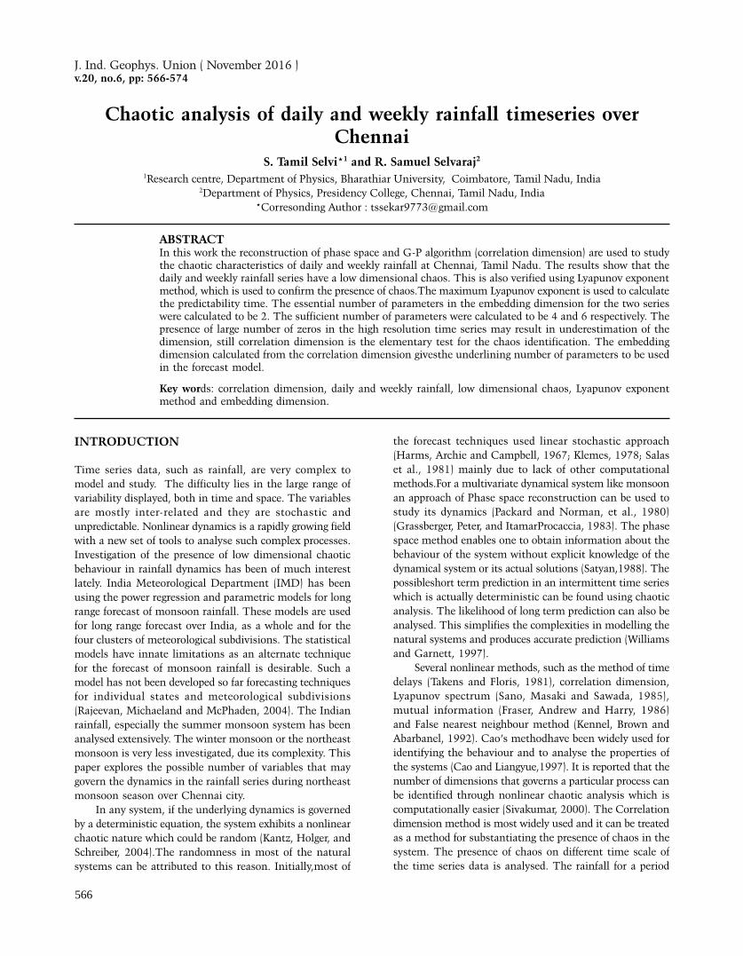
Chennai daily rainfall time series data are used for analysis. The number of data point is 3907 daily total with 45% of nonzero values in it. Figure 1a shows the time series plot for the daily rainfall data.Even though there are prominent peaks observed in the plot, the irregular behaviour of the series does not indicate whether the series is deterministic, stochastic or chaotic. Inorder to analyse the daily rainfall data, a graph is plotted by considering the number of rainy days in each year (Figure 1b) and another plot is made for the total amount of rainfall received in each year (Figure 1c).

Figure 1a. Time series plot of Chennai Daily rainfall (mm).

Figure 1b. A plot for the number of rainy days from 1971-2013.

Figure 1c. A plot for the amount of rainfall received from 1971-2013.


569

The trendline in the plot clearly shows that the number of rainy days increases (increasing trend) and at the same time the intensity (amount) of rainfall decreases (decreasing trend). Chennai has experienced particularly heavy rains roughly once every 10 years—1969, 1976, 1985, 1996, 1998, 2005 and 2015.

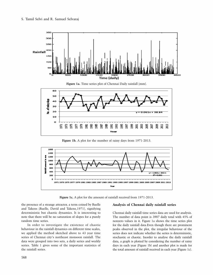
Further investigation is done using the correlation dimension.The time delay was calculated using the Average Mutual Information (AMI) function using the Visual recurrence analysis (VRA).The delay coordinate for Chennai daily rainfall series was 8.

Figure 2 shows the AMI chart for the daily series. The correlation sum and the correlation exponent were calculated using the R statistical software. Figure 3 shows the correlation sum for daily rainfall data for a time delay of 8. The correlation exponent increases with increase in embedding dimension up to a certain value and saturates further. The saturation value of the correlation dimension dc =0.487. This indicates the presence of a low dimension attractor in Chennai daily rainfall series. The dimension of a reconstructed phase space can be estimated from Takens (1981) embedding theorem. It was calculated to be 1.974.

Figure 2. Average mutual information for estimating time delay calculation.

Figure 3. Correlation sum for daily rainfall series for different embedding dimension (m=1 to m=10).

Figure 4. Reconstructed phase space for Chennai daily rainfall.


570

A reconstructed space phase for the daily rainfall series is in two dimension with m=2, time delay t= 1 is shown in Figure 4. The projection of attractor on the plane {Xi, Xi+1} is shown here. It can be inferred from the figure that the projection does not show a clear well defined attractor. Also it is not scattered over the entire region of phase space. The Figure 4 suggests that the dynamics of Chennai city rainfall exhibits intermediate level of complexity.

The estimation of embedding dimension, m, was further verified by the False Nearest Neighbour (FNN) method using Visual Recurrence Analysis (VRA). The value from FNN method was estimated to be m=1. The saturation value of the correlation exponent presented in Figure 5 occurs at m= 4. This value of saturation provides the upper bound of phase space sufficient to describe the dynamics of the attractor. According to the theory of non-linear dynamics, the dimension of the phase space is equal to number of variables present in the evolution of the system. Thus in the analysis of the Chennai daily

rainfall series, the low dimensional attractor in it can be modelled with minimum number of essential variables equal to 2 and number of sufficient variables is 8. Thus on a small temporal scale the rainfall dynamics shows persistence.

Analysis of Chennai weekly rainfall series:

Chaotic analysis was performed using the time series for the weekly rainfall data. The data from Thursday to Wednesday (meteorological week in use in IMD) were aggregated to form the weekly data. Figure 6 shows the weekly rainfall data record.

The total number of samples is 558 with 83 % of non-zero values in it. The average mutual information function for the weekly time data is shown in the Figure 7. It is clear from the figure that the there is a complete loss of information after two weeks indicating it is an optimal time delay.

Figure 5. Relation between correlation dimension and Embedding dimension for Chennai daily rainfall series.

Figure 6. Time series plot of Chennai weekly rainfall.

Figure 7. Time lag by average mutual information function for weekly rainfall.


571

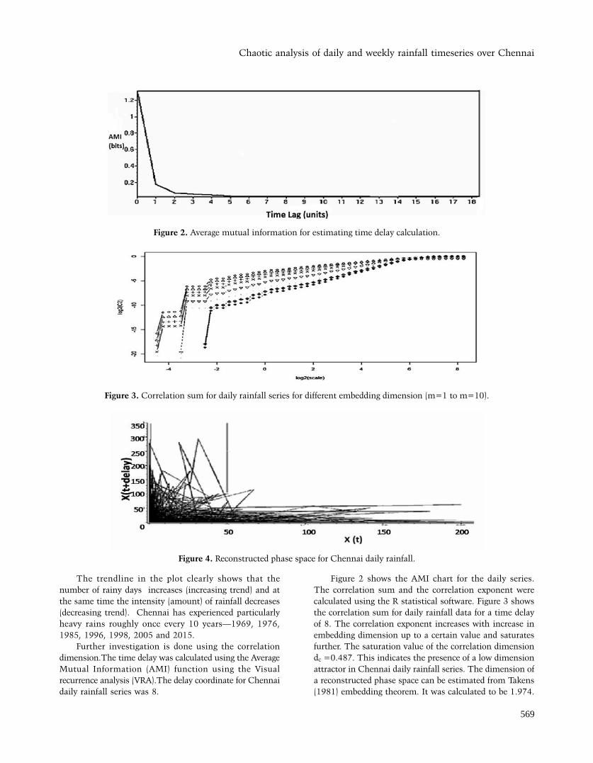
The correlation sum for the weekly rainfall data is shown in Figure 8. The relationship between the correlation exponent and the embedding dimension for the reconstructed phase space is shown in Figure 9. The correlation exponent increases with increase in the embedding dimension up to a certain value and saturates at dc = 0.655.Thus the sufficient embedding dimension for describing the system as per Taken’s (1981) theorem was found to be 2.31.

The saturation value of the correlation exponent presented in Figure 9 occurs at m= 6. This value of saturation provides the upper bound of phase space

sufficient to describe the dynamics of the attractor. According to the theory of non-linear dynamics the dimension of the phase space is equal to the number of variables present in the evolution of the system.

Thus in the analysis of the Chennai daily rainfall series, the low dimensional attractor in it can be modelled with minimum number of essential variables equal to 2 and number of sufficient variables is 8. Thus on a small temporal scale the rainfall dynamics shows persistence. The essential number of variables required for the evolution of the system is same for both daily and the weekly rainfall, unlike the 8 parameter model used by Guhathakurta et al.,(1999).

Figure 8. Correlation sum graph for the weekly rainfall.

Figure 9. Relation between embedding dimension and correlation integral for weekly rainfall.

Figure 10. Phase space reconstruction for weekly rainfall.


572

In order to study monsoon rainfall, two parameters are sufficient to model the station rainfall.The two dimensional reconstructed phase space plot is shown in Figure 10. In comparison to the phase space plot of thedaily series, the weekly series shows quite a good spread over the phase region and the presence of number of zeros that influenced daily rainfall has considerably reduced in the weekly rainfall.

Lyapunov exponent

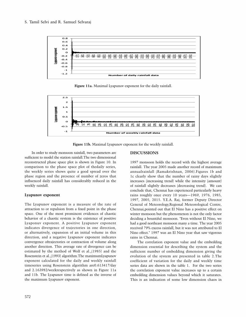
The Lyapunov exponent is a measure of the rate of attraction to or repulsion from a fixed point in the phase space. One of the most prominent evidences of chaotic behavior of a chaotic system is the existence of positive Lyaponuv exponent. A positive Lyapunov exponent indicates divergence of trajectories in one direction, or alternatively, expansion of an initial volume in this direction, and a negative Lyapunov exponent indicates convergence oftrajectories or contraction of volume along another direction. This average rate of divergence can be estimated by the method of Wolf et al.,(1985) and the Rosenstein et al.,(1993) algorithm.The maximumLyapunov exponent calculated for the daily and weekly rainfall timeseries using Rosenstein algorithm are0.613417/day and 2.163982/weekrespectively as shown in Figure 11a and 11b. The Lyapunov time is defined as the inverse of the maximum Lyapunov exponent.

DISCUSSIONS

1997 monsoon holds the record with the highest average rainfall. The year 2005 made another record of maximum annualrainfall (Ramakrishnan, 2006).Figures 1b and 1c clearly show that the number of rainy days slightly increases (increasing trend) while the intensity (amount) of rainfall slightly decreases (decreasing trend). We can conclude that, Chennai has experienced particularly heavy rains roughly once every 10 years—1969, 1976, 1985, 1997, 2005, 2015. Y.E.A. Raj, former Deputy Director General of Meteorology,Regional Meteorological Centre, Chennai,pointed out that El Nino has a positive effect on winter monsoon but the phenomenon is not the only factor deciding a bountiful monsoon. "Even without El Nino, we had a good northeast monsoon many a time. The year 2005 received 79% excess rainfall, but it was not attributed to El Nino effect." 1997 was an El Nino year that saw vigorous rains in Chennai.

The correlation exponent value and the embedding dimension essential for describing the system and the sufficient number of embedding dimension giving the evolution of the system are presented in table 2.The coefficient of variation for the daily and weekly time series data are shown in the table 1. For the two series the correlation exponent value increases up to a certain embedding dimension values beyond which it saturates. This is an indication of some low dimension chaos in

Figure 11a. Maximal Lyapunov exponent for the daily rainfall.

Figure 11b. Maximal Lyapunov exponent for the weekly rainfall.


573

the system. The correlation exponent value for the daily and weekly series are 0.487 and 0.655 respectively. The corresponding embedding dimension value for the two series is 1.97 and 2.31 (Table 2). This value gives the number of essential variables required to study the Chennai rainfall dynamics as 2 and the sufficient number of variables involved in the evolution of the system is 4 for daily series and 6 for weekly series.

The irregularity of the values in the time series can be represented by correlation dimension. A series with high(low) variability in values provides a higher(lower) dimension, which in turn, indicates higher(lower) complexity in the dynamic of the process. From the above results the variability of the rainfall for the two series is not seen explicitly. In nature the temporal accretion of the rainfall often decreases the variability. The values of the coefficient of variation in Table 2 also support the above point.

The phase space trajectory alone does not imply a chaotic system, hence, the need for further investigation arises. An indicator of nonlinearity in dynamical or time series data is the Lyapunov exponent. A positive Lyapunov value is an indicator of chaos. Chaotic system is strongly sensitive to initial value. TheLyapunov exponent predictability time gives the forecasting period up to which we can get reliable forecast. The maximum Lyapunov exponent is calculated for the daily and weekly rainfall time series as 0.613417 and 2.163982 respectively. This implies that the system is unstable and chaotic. The Lyapunov time is defined as the inverse of the maximum Lyapunov exponent. For the above system, the value of Lyapunov time is 1.630 and 0.462 for the daily and weekly rainfall respectively. This indicates the prediction time after which the system starts to behave in a chaotic manner.

CONCLUSIONS

Using the correlation dimension value, the rainfall dynamics of the Chennai city rainfall was examined for two temporal scales, daily and weekly. The principal assumption was that the influence of the presence of zeros in the rainfall series will be minimised if a different temporal scale is chosen. The result provided evidence that the rainfall dynamics can be characterised by deterministic chaos. The correlation dimension value for the daily and weekly rainfall series were 0.487 and 0.655 respectively. This suggests that

there is a low dimension chaos prevailing in the dynamics of the system. Also the essential number of variables for the evolution of the system is 2 for both the temporal scales and the sufficient number of the variables required for the evolution of the system is 4 and 6 respectively. Thus the correlation dimension method serves as a basic step in chaos identification. The selection of number of parameters to model the rainfall dynamics in India is always a debatable issue. The correlation dimension method helps to identify the exact number of variables involved in the evolution of the system. An important limitation in the present analysis is the presence of large number of zeros. This may result in the underestimation of the correlation dimension. Thus the presence of chaos is confirmed by one of the non-linear test such as Lyapunov exponent method, to strengthen the current result. Therefore, we conclude that daily and weekly forecast can be preparedfor short to medium time scale, due to its intrinsic complexity. From the analysis results, we arrive at a conclusion that the dynamical behaviour of Chennai daily and weekly rainfall has a low-dimensional chaos and hence, long term prediction is nearly impossible.

ACKNOWLEDGMENTS

Thanks are due to Dr. T.V. Lakshmi Kumar and Dr.O.P.Singh for constructive suggestions and objective reviewing. They also thank Dr.Nandini Nagarajan for apt editing of the manuscript.

Compliance with Ethical Standards

The authors declare that they have no conflict of interest and adhere to copyright norms.

REFERENCES

Cao, and Liangyue, 1997. "Practical method for determining the

minimum embedding dimension of a scalar time series."

Physica D: Nonlinear Phenomena 110.1, pp: 43-50.

Fraser, Andrew M., and Harry L. Swinney, 1986. "Independent

coordinates for strange attractors from mutual information."

Physical review A 33.2, pp: 1134.

Grassberger, Peter, and Itamar Procaccia, 1983. "Characterization

of strange attractors." Physical review letters 50.5, pp: 346.

Table 2. Correlation dimension result for the rainfall data on different temporal scales.

Parameters Daily rainfall Weekly rainfall

Correlation dimension 0.487 0.655

Delay time 8 2

Essential embedding dimension 1.97 ~ 2 2.31 ~ 2

Sufficient embedding dimension 4 6


574

Guhathakurta, P., Rajeevan M., and Thapliyal V., 1999. "Long

Range Forecasting Indian Summer Monsoon Rainfallby

a Hybrid Principal Component Neural Network Model."

Meteorology and atmospheric physics 71.3-4, pp: 255-266.

Harms, Archie A., and Thomas H., Campbell, 1967. "An extension

to the Thomas-Fiering Model for the sequential generation

of streamflow." Water Resources Research 3.3, pp: 653-661.

Henderson, H.W., and Wells, R., 1988. Obtaining attractor

dimensions from meteorological data. Adv. Geophys, v.30,

pp: 205–237.

Kantz, Holger, and Thomas Schreiber, 2004. Nonlinear time series

analysis. Cambridge university press, v.7.

Kennel, M., Brown, R., and Abarbanel H., 1992. “Determining

embedding dimension for phase-space reconstruction using

a geometrical construction”.Physical Review A, v.45, no.6

pp: 3403-3411.

Klemes, V., 1978. "Physically based stochastic hydrologic analysis."

Advances in hydroscience 11, pp: 285-356.

Packard, and Norman H., et al., 1980. "Geometry from a time

series." Physical review letters 45.9, pp: 712.

Rajeevan, M., Michael J., and McPhaden, 2004. "Tropical Pacific

upper ocean heat content variations and Indian summer

monsoon rainfall." Geophysical research letters 31.18.

Ramakrishnan, T., 2006. Entering 2006, city reservoirs filled to

the brim, Jan. 3, 2006- Retrived from “The Hindu”.

Rosenstein, M. T., Collins J. J., and De Luca, C. J., 1993. "A

practical method for calculating largest Lyapunov exponents

from small data sets." Physica D, v.65, pp: 117-134.

Ruelle, David, and Floris Takens, 1971. "On the nature of

turbulence." Communications in mathematical physics

20.3, pp: 167-192.

Salas, Jose D., Ricardo A., and Smith, 1981. "Physical basis

of stochastic models of annual flows." Water Resources

Research 17.2, pp: 428-430.

Sano, Masaki, and Yasuji Sawada, 1985. "Measurement of the

Lyapunov spectrum from a chaotic time series." Physical

review letters 55.10, pp: 1082.

Satyan, V., 1988. "Is there an attractor for the Indian summer

monsoon?" Proceedings of the Indian Academy of Sciences-

Earth and Planetary Sciences 97.1, pp: 49-52.

Sivakumar B., 2000. "Chaos theory in hydrology: Important issues

and interpretations". J. Hydrol., v.227, pp: 1-20.

Takens and Floris, 1981. "Detecting strange attractors in turbulence."

Dynamical systems and turbulence, Warwick 1980. Springer

Berlin Heidelberg, pp: 366-381.

Williams and Garnett P., 1997. Chaos theory tamed. Joseph

Henry Press.

Wolf A., Swift, J.B., Swinney, H. L., and vastano, J.A., 1985.

"Determining Lyapunov exponents from a short time series."

Physica D, v.16, pp: 285-317.

Chaotic analysis of daily and weekly rainfall … 20-6 (web)/paper6.pdfChaotic analysis of daily and...

Documents

Transcript of Chaotic analysis of daily and weekly rainfall … 20-6 (web)/paper6.pdfChaotic analysis of daily and...