Channel Design and OEM Growth in a Multi-market Setup

Channel Design and OEM Growth in a Multi-marketSetup

Hsiao-Hui Lee† • Tingkai Chang‡ • Kevin Jean£ •Chia-Wei KuoΓ,1

Department of Management Information Systems, National Chengchi University, Taipei,

Taiwan, [email protected]†

Department of Business Administration, National Taiwan University, Taipei, Taiwan,

[email protected]‡, [email protected]£, [email protected]Γ

April 2021

Abstract. We study how to design an original equipment manufacturer’s (OEM’s) direct selling channel

in a multi-market setup such that the OEM experiences sustained business growth without sacrificing its

brand customers’ profits. In this paper, we consider an OEM producing for a brand customer that operates

in two markets: the domestic market in which the OEM resides and the international market (i.e., other

mature markets). The OEM can offer its brand customers at a discount price in exchange for using the excess

capacity to produce products under the OEM’s own brand and then sell these products through its channel.

We build a game theoretical model in a Stackelberg setting in which the OEM is the leader and the brand is

the follower, and determine their optimal pricing decisions and the associate profits under two different dual

channel settings (i.e., one in which the brand cannot flexibly change its retail price and one in which it can).

Contrary to the first-order intuition of market cannibalization, we find that the OEM direct selling channel

can be a win-win-win strategy for the brand (gaining higher profit margin in the international market), the

OEM (gaining a higher market coverage in the domestic market), and consumers in the domestic market

(buying the product at a cheaper price). Such insights are generally robust, even when we consider a cost

for the OEM’s selling channel, and/or consider a price constraint enforced by the brand, such that the OEM

avoids selling the same product at too low a price.

Keywords: Supply chain management; channel of distribution; incentives and contracting; market expan-

sion.

1 Corresponding Author. (T)+886-2-3366-1045, (F)+886-2-2362-5379

1

1 Introduction

Global sourcing has become ubiquitous in present business environments, thus leading to

more and more dispersed supply chains that spread across different continents, as well as

creating both challenges and opportunities for firm growth. Stan Shih, the founder of Acer,

Inc., which specialized in personal computers, observed that parties at both ends of a supply

chain (i.e., design and innovation as well as branding and service) received more value-added

benefits than those parties in the middle (i.e., manufacturing and production). This U-

shaped relationship, denoted as a smile curve (Shih 1996), suggests that original equipment

manufacturers (OEMs) often receive fewer profit shares than their brand partners. One

growth option for OEMs is to expand their market coverage by offering their own brand

products. However, such a business expansion option is risky; because of market cannibal-

ization, these OEMs’ brand customers may suffer from lower profits and, hence, may decide

not to continue their business with these OEMs. In this paper, we discuss how adding an

OEM selling channel in a “multi-market” setup can help increase an OEM’s market coverage

and profitability, while maintaining its relationship with its brand customers by providing

the same, if not more, profits to these brands via economies of scale.

As a motivating example, we use the case written by Ng et al. (2010) that illustrates

the growth of Galanz Enterprises Group Co. Ltd., an OEM for major international brands’

microwave ovens in China. In the mid 1990’s, prices of microwave ovens with international

brands (e.g., Panasonic, Toshiba) in China ranged from RMB 1,000 to 3,000; however, per

capita annual income of urban households in 1995 was only around 4,200 RMB. During

this period, while serving as an OEM for these international brands, Galanz started selling

products carrying its own brand in China at a low price (as low as RMB 300 per unit).

To achieve this low price strategy and stay competitive in the market, Galanz adopted

production line transfer agreements with its international brand customers, so it could freely

use its excess capacity to sell its own brand’s low-price microwave ovens in China. In return,

Galanz significantly lowered its wholesale price to these international brand customers. Using

2

economies of scale to lower production costs, Galanz sold more than 16 million microwave

ovens and earned 76% of the Chinese market (denoted as the domestic market) by October

2000. We note that this type of business model, which leverages an OEM’s low cost strategy

and economies of scale in setting its own brand (and/or selling channel), is not uncommon

even to this day. For example, Foxconn, one of Apple’s largest OEMs, produced smart

phones under its new brand2 with its partner HMD in 2019.3 According to Neil Mawtson,

wireless devices executive director at Strategy Analytics, “HMD smartphone models deliver

relatively high specs at relatively reasonable price points.” In 2019 Q2, HMD shipped 4.8

million Nokia smartphones, a 55% growth in shipments compared to Q1 2019 or 20% growth

to Q2 2018.4

In ways that differ from the dual channel literature that considers OEMs and brands

competing in the same market to highlight the cannibalization effect, we focus on two aspects

that capture an OEM’s challenges: brand-OEM relationship and market structure. First,

depending on incentive terms, brand customers that had been working with the OEM (e.g.,

Panasonic or Toshiba in the Galanz case) may not agree with the OEM’s own selling channel,

as these brands often have concerns over cannibalization in the domestic market (e.g., the

Chinese market in the case). Therefore, incentives to brands are needed to overcome brand

customers’ concerns over intensified competition. As an example, when Galanz initiated

its low-price strategy, most of its customers could not follow such a low price, and they

were either pushed out of the Chinese market or only focused on loyal consumers who only

purchase brand products. In order to mitigate this issue, Galanz offered a very low wholesale

price to its customers, who, in turn, received a higher premium for products sold outside

2 Nokia has licensed Foxconn to use its brand name for ten years.

3 https://www.forbes.com/sites/ralphjennings/2019/01/31/apple-contractor-foxconn-makes-gains-with-

its-own-brand-of-phones-in-a-tough-market/68fde0f22c48

4 https://nokiamob.net/2019/07/31/nokia-smartphone-sales-rebound-with-4-8-million-units-shipped-in-

q2-2019/

3

China. As a result, these customers still continue their sourcing relationship with Galanz

despite the market cannibalization effect within the China market.

Second, although OEMs can use a low wholesale price strategy to incentivize brand

customers’ agreements and reduce potential business friction, the market structure still plays

an important role. In particular, we consider multiple markets: the international markets in

which brands operate, and the domestic market in which both the brands and OEMs operate.

For example, during Galanz’s rising period, China was considered the “world’s factory” but

not the “world’s market.” These customers, even though they were pushed to give up this

(small) market, did not seem to mind the intensified competition, as Galanz’s wholesale price

helped them obtain a heavy margin from other markets in which they operated. However,

as the Chinese market grew further, some of these brands returned to this market, but no

longer sourced products from Galanz, as sourcing from Galanz sustained Galanz’s low cost

strategy (due to increased scales) and, hence, intensified competition. As a result, in addition

to the multi-market assumption, market characteristics of the domestic market play a key

role with respect to both brands’ and OEMs’ decisions.

Motivated by the Galanz example, we model a supply chain with an OEM and a brand

that can sell the product to two markets: the domestic market (where the OEM is located)

and international markets (other countries). In a conventional supply chain (denoted as

Channel B), the OEM sells products to the brand, and then the brand distributes the goods

to consumers in both markets. In contrast, the OEM can also sell products in the domestic

market with its own brand name at a lower price than the brand, and then sell products

to the brand with a lower wholesale price than that in Channel B to induce the brand’s

agreement, so the OEM may use its excess capacity. In this case, the OEM operates a dual

channel, but only competes with the brand in the domestic market.

To further model how market characteristics influence the brand and the OEM’s decision,

we consider three components: the size of the international market, the size of the domestic

market, and the size of the brand’s loyal consumers in the domestic market. As the product

under the brand’s name has the same quality as the one under the OEM’s name, consumers

4

will likely purchase the OEM’s product, as long as the price of the OEM product is lower.

However, in emerging markets, some consumers perceive brand names differently (e.g., rich

consumers in an M-shaped society), and these consumers will only purchase brand products

as long as they can afford these products. In this paper, we identify this group as “loyal

consumers”who view a brand as an indicator of perceived quality (instead of valuing only

the physical quality, which is the same as mentioned previously)5.

Motivated by the above-mentioned issues, we pose the following research questions. How

can the OEM design a direct selling channel serving different markets without objections

from its brand customers? Can this direct selling channel be beneficial to the OEM, the

brand, and consumers, simultaneously? To answer these questions, we first consider the

situation in which a brand maintains its pricing strategy even after the OEM’s direct selling

channel is established (denoted as Channel C). This situation is largely consistent for brands

that enter the domestic market but try to maintain their branding effect.6 In this case, we

show that Channel C always achieves a higher supply chain profit (sum of the profits of the

brand and the OEM) than Channel B when the domestic market is not too small.7 Moreover,

the brand receives the same profit as that of Channel B, such that it is indifferent to such a

dual channel; even though the sales from the domestic market are reduced, the high margin

5 Prior research on brand effect provides supporting evidence that good brand names have a positive

effect on perceived quality (e.g., see Grewal et al. 1998, Rao and Monrow 1989, and Dodd et al. 1991).

6 For example, brands like Apple and Microsoft may likely keep their respective pricing strategies. For

example, the price of an iPhone X (64 GB ROM) is 999 USD in the US, 1,023 USD in Japan, 1,215 USD

in China, and 1,211 USD in Switzerland. Excluding import taxes, these prices are very compatible.

We used exchange rates of 113.05 for JPY to USD, 6.9 for RMB to USD, and 1.001 for CHF to USD

(accessed date November 4, 2018). Moreover, as shown in Grewal et al. (1998), price discount has a

negative effect on consumers’ internal reference prices; thus, some brands, though they can, may not

be willing to lower their respective prices when entering a new market.

7 When the domestic market is too small such that the brand only operates in the international market,

the OEM does not want to offer its own product, as the domestic market cannot sustain its selling

channel.

5

derived from the low wholesale price compensates for this loss.8 The OEM receives higher

profits from increased sales in the domestic market. We also show that with the additional

channel, the OEM also increases total production scale (i.e., sum of both the sales under

its name and sales under the brand’s name). As an added benefit, the increased production

scale results solely from the domestic market, and because more consumers in the domestic

market can enjoy a low-price product, such a channel design improves social welfare as well.

Second, we relax the brand’s fixed pricing and allow the brand to change its retail price

after the entry of the OEM’s direct selling channel (denoted as Channel F). Some brands can

react to the OEM’s low-price product by re-optimizing their respective pricing strategies.

Intuitively, this additional flexibility with respect to brand pricing enables the brand’s power;

as a result, we expect this added flexibility to hurt the OEM’s profit. Contrary to our first-

order intuition and under minor conditions, when the domestic market is sufficiently large,

Channel F still always outperforms Channel B with respect to OEM profit (and, hence,

supply chain profit). Interestingly, for a sufficiently large domestic market and a small

portion of loyal consumers, the brand also lowers its retail price in the international market

and orders more from the OEM, further enabling the OEM to use scale to lower costs. As an

added benefit, the OEM’s production scale increment in Channel F results not only from the

domestic market but also from the international market, thereby improving social welfare.

In addition to comparing the single channel (Channel B) with the dual channels (Channels

C and F), we also use this paper to analyze when the flexible retail price is preferred by the

OEM. In a sufficiently large domestic market, the OEM benefits more from the brand’s

flexible retail price due to the brand’s higher sales in the international market. However,

these benefits diminish in smaller domestic markets, and the supply chain prefers a fixed

8 Our model can be easily modified to allow a brand to charge a (fixed) authorization fee. As long as the

improved supply chain profit exceeds this fee, supply chain profits can be freely distributed between the

brand and the OEM, and managerial insights remain with only slight changes with respect to domestic

market thresholds.

6

brand price in equilibrium when the domestic market is sufficiently small. Furthermore, the

size of the loyal consumer base in the domestic market also significantly affects equilibrium

strategies. A large portion of loyal consumers makes it easier for the OEM to provide the

same profit to the brand under dual channels, but it also reduces the market size for the

OEM. This mixed effect complicates our analysis in ways that yield some interesting results:

the profit in Channel C increases with the number of loyal consumers, whereas the profit in

Channel F decreases with the number of loyal consumers.

Finally, we include two extensions. In the first, we aim to capture both the situation in

which a customer can also write contract terms to limit the OEM’s retail price, as well as the

situation when the OEM incurs a cost by operating its own channel. Generally, adding these

two constraints make it difficult for the OEM to maintain a dual channel. Hence, one can

expect the entire supply chain to incline more towards Channel B in this extension. However,

as we show in our numerical results, our previous insights still remain for a wide range of

parameters for both the price constraint and operations costs. In the second extension, we

analyze a model with a quality-embedded utility function to capture the potential vertical

quality differentiation between the brand’s and the OEM’s respective products. In this

extension, we no longer assume a fixed portion of loyal consumers but allow consumers with

different valuation toward quality and prices to select the channel from which they should

purchase, based on their utility comparison. We find that although Channel C is degenerated

to Channel B, Channel F strictly outperforms Channel B, thus leading to a similar insight

as that obtained with our main model.

Our work contributes to the operations literature by analyzing how a dual channel can

be used to sustain firm growth in a multi-market setup. Our work focuses on how market

structure (i.e., the sizes of the two markets and loyal consumers) affect dual channels and

pricing decisions. Specifically, our analytical outcomes not only help explain how parties’

behaviors in supply chains depend upon market characteristics, but also how OEMs can

use a proper channel design to create a win-win situation for themselves and their brand

customers. To enhance their profits, OEMs can persuade their brand customers (using

7

lowered wholesale prices) to allow them to operate their own selling channels. Depending on

how mature the domestic market is and how many consumers are at the top of the pyramid,

these OEMs can also influence their brands’ decisions in modifying their pricing strategies.

Moreover, our work offers the following managerial insights and suggested actions. When

an OEM grows, it must consider the transition from an OEM business to an OBM business

by setting up its own brand and/or selling channel. However, a typical challenge is whether

such a move creates an internal conflict of interests between its OEM business and its OBM

business, as the brands that source products from this OEM may deter the OEM’s move

by threatening the OEM to remove their orders. 9 Our result suggests both conditions and

ways for OEMs to grow under such a challenge. Specifically, it is easier for OEMs that sell to

brands with a sales focus on other developed markets than emerging ones (where the OEMs

operate) to persuade their brand customers by leveraging their economies of scale and low

cost strategies. By compensating brands for their losses in the domestic market, the brands

gain higher profit margins and/or higher international market coverage. Moreover, supply

chain profits may also be freely distributed to brands by using channel authorization and

licensing fees paid by OEMs to further incentivize the brands and create a win-win situation

for both parties. Finally, given different market structures, OEMs can also incentivize their

brand customers to either adjust their retail prices or not to maximize their entire supply

chain profits. Finally, we note that our work also has implications with respect to consumer

welfare. By understanding when and how to establish OEM dual channels, consumers in

emerging countries may enjoy low-cost alternatives that they could not previously afford,

and policy makers might consider incentive schemes to help cultivate the growth of such

OEM businesses, should doing so benefit their people.

We organize the remainder of this paper as follows. After we review the existing literature

in Section 2, we use Section 3 to outline our model and present our analytical results. Section

4 compares the dual channels and consider the case in which the brand is able to offer

9 This has been shown to be a great challenge for many firms, such as ASUS (Shih et al. 2010).

8

differential pricing for both markets and own the OEM production in our comparison. In

Section 5, we provide two extensions of our model. We conclude our paper in Section 6 with

a discussion and some directions for future research. We provide all proofs in the Appendix.

2 Literature Review

Our work is closely related with the channel design literature that focuses upon a supply

chain comprised of a manufacturer and a retailer. By optimizing pricing and other decisions,

these works generally focus on channel efficiency by comparing profits (including the supply

chain as well as the players in the chain) under the traditional retail channel and under

the dual channel. For example, Tsay and Agrawal (2004) consider a setting in which a

manufacturer can initiate a direct sales channel, which may not hurt the retailer. They

provide a thorough discussion regarding different sources of inefficiencies, such as double

marginalization and channel conflicts, and how to mitigate these adverse effects in the dual

channel. In addition to pricing decisions, some other studies analyze how a manufacturer or a

retailer in a dual channel makes decisions with respect to the timing of pricing (Matsui 2017),

product assortment (Rodrıguez and Aydın 2015), and leadtime (Hua et al. 2010; Modak and

Kelle 2019). Yan (2020) further extends the dual-channel setting to online finance services,

and Xiao and Shi (2016) consider a dual-channel setting for which supply shortage may exist

in the channel.

Most studies in the channel design literature consider cases in which a manufacturer can

freely establish a direct selling channel, regardless of a retailer’s preference. Indeed, in some

scenarios, a dual channel can be a win-win for both the manufacturer and the retailer, and

hence the manufacturer can freely operate its own channel (e.g. Chiang et al. 2003; Cattani

et al. 2006; Arya et al. 2007; Cai 2010; Vinhas and Heide 2014; Xiao et al. 2014; Ha et

al. 2015; Caidieraro 2016; Chen et al. 2017; Yan 2019; Matsui 2020). For example, Chiang

et al. (2003) suggest that when consumers have a low preference toward a direct selling

channel, such a channel design benefits both the manufacturer and the retailer. Cattani

9

et al. (2006) find that when the manufacturer can optimally choose the wholesale and

retail prices (instead of fixing either of these prices), such a channel design also benefits the

retailer. Arya et al. (2007) consider a higher direct channel cost, and demonstrate that

manufacturers and retailers can benefit from such a dual channel when manufacturers can

lower wholesale prices offered to their retailers, thereby lowering the double marginalization

issue. Although we find many cases in which both the manufacturer and retailer benefit from

the direct selling channel, numerous cases also suggest that adding a new channel still incurs

double marginalization that hurts all parties. For example, extending the work of Arya et

al. (2007), Li et al. (2014) consider the case that only the retailer possesses information

regarding market size, and this information asymmetry leads to a poor performance for not

only the retailer, but also for the manufacturer under a dual channel design, especially in

smaller markets.

In addition, many dual channel studies assume that consumers’ utility function is purely

based on the prices set by each channel (e.g., Cattani et al. 2006; Dumrongsiri et al. 2008;

Mukhopadhyay et al. 2008; Ha et al. 2015; Yu et al. 2017; Chen et al. 2017), except that

some explicitly model consumer channel-specific preferences (either an explicit preferences

or via differential product qualities). In addition to price comparison considerations, Chiang

and Monahan (2005), Geng and Mallik (2007), and Chiang (2010) also consider that a good

number of consumers prefer to search for and buy products online (i.e., “direct channel”

in our paper). In a two-manufacturer and two-retail channel setting, Dukes et al. (2006)

consider the case that consumer preferences depend on the combination of manufacturers

and retailers (i.e., a total of four channels). Considering multiple retailers, David and Adida

(2015) assume that some consumers prefer each type of retailer, regardless of price. Matsui

(2016) shows asymmetric product distribution may exist in equilibrium, even when both

manufacturers are symmetric. Iyer (1998), following assumptions similar to ours, also models

brand loyalty when consumers make their purchase decisions.

Our paper differs from those in the extant literature in two aspects: brand-OEM rela-

tionship and market structure. First, our paper considers the mitigation of channel conflicts

10

between an OEM and a brand. Upon initiating the direct channel to serve the domestic

market, the OEM makes pricing decisions (both its own retail and wholesale prices) so that

the brand will earn at least the same profit that it would earn in a single channel. Second, the

existing literature mainly considers a single market setup (e.g., Chiang et al. 2003; Netessine

and Rudi 2006; Arya et al. 2007; Li et al. 2014; Ha et al. 2015). In our paper, the OEM only

sells its products to the domestic market, whereas the brand serves the international market

as well as loyal consumers in the domestic market who prefer to purchase from the brand

as long as the products are affordable. This setup enables us to incorporate the channel

preference captured by the prior literature, as well as the dual market setup that has not yet

been explored in previous studies. We are particularly interested in how the characteristics

of these two market segments (domestic and international) and loyal consumers influence

channel pricing decisions and channel efficiency, so we may better understand how an OEM

can design its selling channel to achieve its market expansion and firm growth.

3 Model and Analysis

We consider a model with an OEM selling a product to a brand owner, who then sells the

product to two markets: a domestic market (where the OEM is located) and an international

market (other countries). The OEM produces the product with unit production cost c, and

sells the product to the brand at a wholesale price w. The brand then sells the product to end

consumers in both markets at the same price p. Because of brand positioning concerns, we

consider that the brand does not price discriminate between the two markets (see Footnote

1, for example). This assumption is generally true for brand products. However, we relax

this assumption in Section 4.3 and investigate channel efficiency when the brand can price

discriminate between the two markets. In this section, we consider three types of channel

designs. First, as a benchmark, we consider that only the brand sells the product to both

markets (denoted as Channel B). Second, we consider that the brand sells its brand products

to both markets but the OEM sells its OEM products only to the domestic market, and the

11

brand cannot adjust its retail price in response to the OEM setting up its selling channel

(denoted as Channel C). Finally, we consider a channel design similar to Channel C, except

that we allow for the brand’s adjustment on retail prices (denoted as Channel F).

Consumers are heterogeneous in their willingness to pay. Hence, we let v be an end

consumer’s willingness to pay, and we assume that v is uniformly distributed in between

[0, α] for the international market and between [0, β] for the domestic market. We consider

β to be sufficiently large (but still smaller than α) so that the brand will be profitable enough

to serve the domestic market.10 We then assume that a consumer with a willingness to pay

v can receive a valuation of v − p if s/he buys the product and his/her reservation value is

0. Therefore, in Channel B for which only the brand offers a selling outlet (differentiated

by a subscript B), the market coverage by a product priced at price pB is α − pB in the

international market and β−pB in the domestic market. The sum of the two then constitutes

the total production scale for the OEM.

However, in the case when the OEM can sell the product directly to the domestic market,

because the product quality is the same (i.e., from the same production line), the valuation

function cannot differentiate consumers who have strong brand loyalty from those who do

not. We model these consumers’ preferences for the brand product (due to perceived better

service or reputation) by a parameter ∆. That is, ∆ high willingness-to-pay consumers

(distributed in between [β −∆, β]) will only purchase the brand product if they can afford

the product. However, if they cannot afford the brand product but can only afford the

OEM product, then they can still buy the OEM product. We denote these high-valuation

consumers as “loyal consumers” in our paper. We do not directly model the perceived

10 First, we consider α > β so that the international market is the main market for the brand. Otherwise,

the brand may pay more attention to the domestic market, and such a case falls outside the scope of

this paper. Second, as long as β − pB > 0, it is profitable for the brand to serve the domestic market.

The inequality can be rewritten as β > (3α+ 2c)/5. We note that, given that α > β, β > (3α+ 2c)/5

also implies c < (α + β)/2, which guarantees the the cost will be sufficiently low enough to allow the

brand to source the product.

12

product quality difference and allow consumers to choose which product to purchase in the

main model for two reasons. First, rich consumers (especially in China, India, and many

emerging economies) do not care about the price difference and only want to buy brand

products. Second, our aim is to investigate how market structure influences an OEM’s

selling channel effectiveness, rather than investigate the effect of quality discrimination for

the perceived product quality through different channels. That said, in Section 5.2, we extend

our main model to consider a quality-embedded utility function that allows consumers to

freely choose the channel, and we find similar insights as those we observe in our main model.

Finally, we refer to the case in which the OEM can sell the product in the domestic

market as “dual channels.” In particular, we consider two brand pricing strategies with

respect to an OEM dual channel: a rigid pricing strategy for which the brand cannot change

its retail prices easily (or at least in the short run) to maintain brand positioning, and a

flexible pricing strategy for which the brand can change its retail prices easily. We denote

the former as Channel C and the latter as Channel F, and differentiate them from Channel

B by using subscripts C and F , respectively. With Channel C, the brand cannot adjust its

original pricing strategy and, hence, its retail price is pC = pB, whereas with Channel F, the

brand can adjust its original pricing strategy fairly easily from pB to pF .

Therefore, when the OEM sells the product in the domestic market, it charges a retail

price of pmi , for which i can be C or F . Following the same consumer valuation logic, we

know that, in the international market where the OEM does not sell its own product, the

brand’s market coverage is α − pi. In the domestic market, the brand’s market coverage

becomes min{∆, β − pi}, depending on how many loyal consumers can afford the brand

product, whereas the OEM’s market coverage becomes β−pmi −min{∆, β−pi}. As a result,

the total market coverage in the domestic market becomes β − pmi . In Table 1, we provide a

summary table of the notations in this paper. In the following subsections, we consider the

case in which the OEM is the Stackelberg leader and the brand is the follower, and analyze

the OEM’s pricing strategies and the associated profits using this assumption.

13

3.1 Channel B: Brand Channel Only

Using the above model setup, we observe that the brand’s profit can be expressed as:

πB = (pB − wB)(α + β − 2pB),

and the OEM’s profit is:

ΠB = (wB − c)(α + β − 2pB).

Solving the two optimizations by the first-order conditions and using backward induction,

we find that the optimal brand retail price is:

pB =3α + 3β + 2c

8.

We denote the optimal brand profit as π∗B and the optimal OEM profit as Π∗B, or,

π∗B =(α + β − 2c)2

32, and Π∗B =

(α + β − 2c)2

16.

3.2 Dual Channels C and F

In Channel C, the brand allows the OEM to establish the OEM’s selling channel, and upon

its establishment, the brand maintains its original retail price pC = pB. In order for the

brand to be incentivized to allow for this OEM channel, the OEM needs to give a wholesale

price wC so that the brand’s profit will not be lower than its original profit, expressed as:

πC = (pC − wC) (α− pC + min{∆, β − pC}) ≥ π∗B.

The OEM also needs to decide its own retail price by maximizing its own profit function,

expressed as:

ΠC = (wC − c) (α− pC + min{∆, β − pC}) + (pmC − c) (β − pmC −min{∆, β − pC}) .

14

As a low wholesale price will increase the brand’s profit but hurt the OEM’s profit, the

OEM sets the wholesale price such that πC = π∗B. We then can solve for the OEM retail

price in Lemma 1.

Lemma 1. The optimal OEM retail price is:

pmC =

β−∆+c

2, if β ≥ 3α+8∆+2c

5≡ β1;

3α+3β+10c16

, if β < β1.

When β = β1, the brand covers exactly the number of loyal consumers in the domestic

market.

This lemma shows that with the dual channel, the OEM can offer a cheaper choice (i.e.,

pmC < pB) to consumers in the domestic market. When β ≥ β1, we obtain:

pB − pmC =3α− β + 4∆− 2c

8> 0,

in which we use α > β and Footnote 10 in the inequality. When β < β1, by using Footnote

10, we obtain:

pB − pmC =3α + 3β − 6c

16> 0.

As a result, this dual channel can successfully price discriminate between the two markets. In

this case, the OEM’s production scale is greatly enhanced, as the market coverage from the

international market remains unchanged, but the market coverage in the domestic market

increased from β − pB to β − pmC , because of the lowered OEM retail price.

In Channel F, the brand allows the OEM to offer a selling channel, but the brand can

adjust its retail price in order to maximize its profit. In this case, in order for the brand to

be incentivized to allow for the OEM channel, the OEM still needs to maintain the brand’s

profit to at least match its original profit (i.e., π∗F = π∗B).11 The profit functions for the brand

11 We can easily show that if the two can freely (optimally) choose their prices, then the brand earns less

15

and the OEM are similar to the ones in Channel C, except that we change the subscript

from C to F , and pF , the brand’s retail price in Channel F, now becomes a decision variable

in addition to pmF . The following lemma characterizes the optimal solution.

Lemma 2. The optimal brand retail price is:

pF =

8α+8∆−

√2(α+β−2c)8

, if β > 8α+16∆−√

2[α−2c]

(8+√

2)≡ β2,

β −∆, if β1 ≤ β ≤ β2,

3α+3β+2c8

, if β < β1.

The optimal OEM retail price is:

pmF =

β−∆+c

2, if β ≥ β1,

3α+3β+10c16

, if β < β1.

First, regardless of the brand’s reaction in its pricing strategy, we observe that the OEM

charges the same retail price. Similar to Channel C, this dual channel also offers a cheaper

choice for the consumer as pmF = pmC < pB, and we therefore know that the OEM also expands

its market coverage in the domestic market in Channel F when compared with Channel B.

However, in the international market, the brand can change its retail price so that pF is

higher than pB. That is, when β < β1, pB = pF , and when β1 ≤ β ≤ β2, we obtain:

pB − pF = ∆− 5β − 3α− 2c

8≤ 0,

because β ≥ β1. When β increases such that β2 < β ≤ βCF , in which,

βCF =(17− 8

√2)α + (24− 8

√2)∆ + c(8

√2− 10)

7,

profit than π∗B . As a result, the OEM still needs to maintain the brand’s profit by lowering its wholesale

price in exchange for the brand’s agreement of the dual channel.

16

then pF ≥ pB. As the brand’s international market coverage changes from α− pB to α− pF

in Channel F, when β is not large (i.e., β1 ≤ β ≤ βCF ), the result, pF ≥ pB, thus implies

that the OEM will lose part of its sales in the international market due to the increased retail

price of the brand. In this case, the brand gains from a higher profit margin in two ways:

from a higher retail price and a lower OEM wholesale price. However, when β is sufficiently

large (i.e., when β > βCF ), the brand is willing to reduce its retail price for larger market

coverage. We use the following corollary to depict the result.

Corollary 1. If β < β1, then pF = pB. If β1 ≤ β ≤ βCF , then pF ≥ pB. If β > βCF , then

pF < pB.

Finally, we compare the overall market coverage of Channel F with Channel B by com-

paring (α+β)−pF −pmF and (α+β)−2pB. If 2pB−pF −pmF > 0, then the overall OEM still

improves its production scale, even though the brand raises its price when β1 ≤ β ≤ βCF .

We have shown above that the inequality is valid when β < β1. When β1 ≤ β ≤ β2, we

obtain:

2pB − pF − pmF =3α− 3β + 6∆

4> 0,

whereas when β > β2, we obtain:

2pB − pF − pmF =2β − 2α− 4∆ +

√2(α + β − 2c)

8> 0,

as this value, obviously, increases with β, and when β = β2, we find that it will be positive

as well, based upon the continuity of this value. Following our collective analysis of these

two lemmas, then, we obtain the following corollary:

Corollary 2. Although Channel C and Channel F both enhance the overall production scale,

the enhancement in Channel F is achieved at the cost of the market coverage in the interna-

tional market when β1 ≤ β ≤ βCF .

Next, we consider how the size of each market, α and β, respectively influences the

optimal retail price decisions (i.e., pB, pC , pmC , pF , and pmF ) in the following lemma.

17

Lemma 3. The following table shows the effects of α and β on the optimal retail price in

the three channels:

Channel B Channel C Channel FpB pC pmC pF pmF

α + +× if β ≥ β1

+ if β < β1

+ if β > β2

× if β1 ≤ β ≤ β2

+ if β < β1

× if β > β1

+ if β < β1

β + + +− if β > β2

× if β < β2+

First, we observe that when the international market size increases (i.e., α increases), it

is always weakly beneficial for both the brand and the OEM retail prices, as these prices are

at least non-decreasing in α. We can observe a similar effect when the domestic market size

increases, except when β > β2 in Channel F. This exception is a result of the brand focusing

more on its market coverage on the international market rather than the profit margin.

4 Effectiveness of Dual Channels

After analyzing the two dual channels (one with a rigid brand price and one with a flexible

price), we next discuss the effectiveness of the two dual channels. We first investigate whether

the two dual channels outperform the single selling channel in Section 4.1. We then compare

the two dual channels to determine which one the OEM prefers in Section 4.2. Finally, as one

benefit resulting from the dual channels is the price discrimination between the two markets

and within the domestic market, we extend the comparison between the dual channels with

a single channel in a centralized system that can price discriminate between domestic and

international markets in Section 4.3. We note that we use supply chain profits as the key

performance for the comparison, as the brand receives the same profit as before; hence, the

OEM profit changes because of the OEM channels are equivalent to the profit changes in

the supply chain.

18

4.1 Comparison between Channel B and Channels C and F

Based on the analysis of the optimal prices in Section 3, we compare the two dual channels

with Channel B in the following proposition:

Proposition 1. (1) Π∗C ≥ Π∗B, and Π∗C weakly increases with ∆. (2) Π∗F ≥ Π∗B, and Π∗F

weakly decreases with ∆ if α is sufficiently large (i.e., α > max{(29− 14√

2)c/(8− 5√

2)−

∆, (24− 7√

2)(∆− c)/(9√

2− 8)}).

First, regardless of the brand’s pricing flexibility, offering a dual channel always benefits

the OEM while maintaining the brand’s profitability, as dual channels can help price dis-

criminate a product. Although some loyal consumers still prefer a brand’s product, the vast

consumers who cannot afford the brand’s product now have a cheaper alternative, as pmC and

pmF are both smaller than pB as we have seen from Lemmas 1 and 2.

Second, Proposition 1 highlights the effect with respect to loyal consumers under different

types of brand pricing flexibility. When the brand cannot adjust its price in the short run

(i.e., Channel C), the OEM benefits from loyal consumers. The number of loyal consumers

influences the OEM profit in two opposite ways. On the one hand, when ∆ increases, the

OEM effective market size (β−∆) shrinks as more consumers in the domestic market would

prefer the brand product over the OEM one. On the other hand, a higher ∆ also makes it

easier for the OEM to offer the same profit to the brand. As the brand has a rigid pricing

strategy, the OEM benefits more from the latter rather than being harmed by the former.

When the brand can flexibly adjust its price (i.e., Channel F), then a higher ∆ reduces

OEM profits, which occurs when the international market size is sufficiently large. This is in

an opposite direction as that demonstrated in Channel C. Flexible brand pricing increases

the power of the brand, as the brand now has a pricing tool (adjusting its own retail price)

to use in supply chain negotiations; moreover, this power is enhanced with a high degree of

attention (i.e., loyal consumers) from the domestic market.

Finally, although we only focus upon the OEM as the Stackelberg leader in the model,

improved OEM profits that result from the dual channel can be easily extracted by the

19

brand. For example, the brand may use a (fixed) authorization fee to allow the OEM to use

excess capacity to produce and sell more products. In this case, the additional profits that

the OEM earned via the dual channel can be freely distributed in the supply chain. As this

process involves the relative bargaining power between the two parties, we do not split the

profits, but rather focus on the enhancement of the OEM’s (and hence, the supply chain’s)

profit.

4.2 Comparison between C and F

Even though we have shown that both dual channel settings always outperform the sin-

gle channel setting because of their ability to price discriminate among consumers, the two

nonetheless differ in their effectiveness. More importantly, understanding the two dual chan-

nels’ relative effects allows the OEM to incentivize the brand to choose the brand’s pricing

strategy, if possible. The difference between the two dual channels’ profits thus gives an

upper bound with respect to the OEM’s incentive amount.

Intuitively, when a brand can adjust its retail prices based on wholesale prices that the

OEM offers, we can expect this extra lever to harm the OEM’s profitability, making it more

difficult for the OEM to incentivize the brand and allow for a dual channel. That said, the

following proposition offers a different result.

Proposition 2. Π∗F > Π∗C if and only if

β > βCF =(17− 8

√2)α + (24− 8

√2)∆] + c(8

√2− 10)

7> β2, (1)

and in this region, pC > pF , whereas pC ≤ pF , otherwise.

First, when the domestic market is mature/large enough, the OEM, and hence the supply

chain, can benefit from the brand’s adjusting its global pricing strategy. This interesting

result (echoing Corollary 1) is due to the improved market coverage, which stems from the

international market. As the proposition shows for this region, pC > pF , implying that

20

the brand lowers its retail prices to both markets. This move neither changes its market

coverage in the domestic market (which is ∆) nor changes the OEM’s market coverage, as

the OEM’s retail prices are the same whether or not the brand can adjust its retail price

(i.e., pmF = pmC ); rather, this move increases the brand’s market coverage in the international

market. Conversely, this proposition also shows that when the domestic market size is small,

the brand usually raises its retail price, knowing that the OEM will offer compensation for

what the brand earns in the single channel setup. Because of this rise in retail price, the

OEM’s profitability and, hence, the supply chain’s profitability will both decrease.

Second, this proposition also shows the effect of loyal consumers in deciding whether

to incentivize the brand to adjust its retail prices. From Equation (1), we see that, when

∆ increases, βCF also increases, implying that Channel F will become less preferred than

Channel C. This result can also be seen from Lemmas 1 and 2: when ∆ increases, Π∗C weakly

increases, but Π∗F weakly decreases.

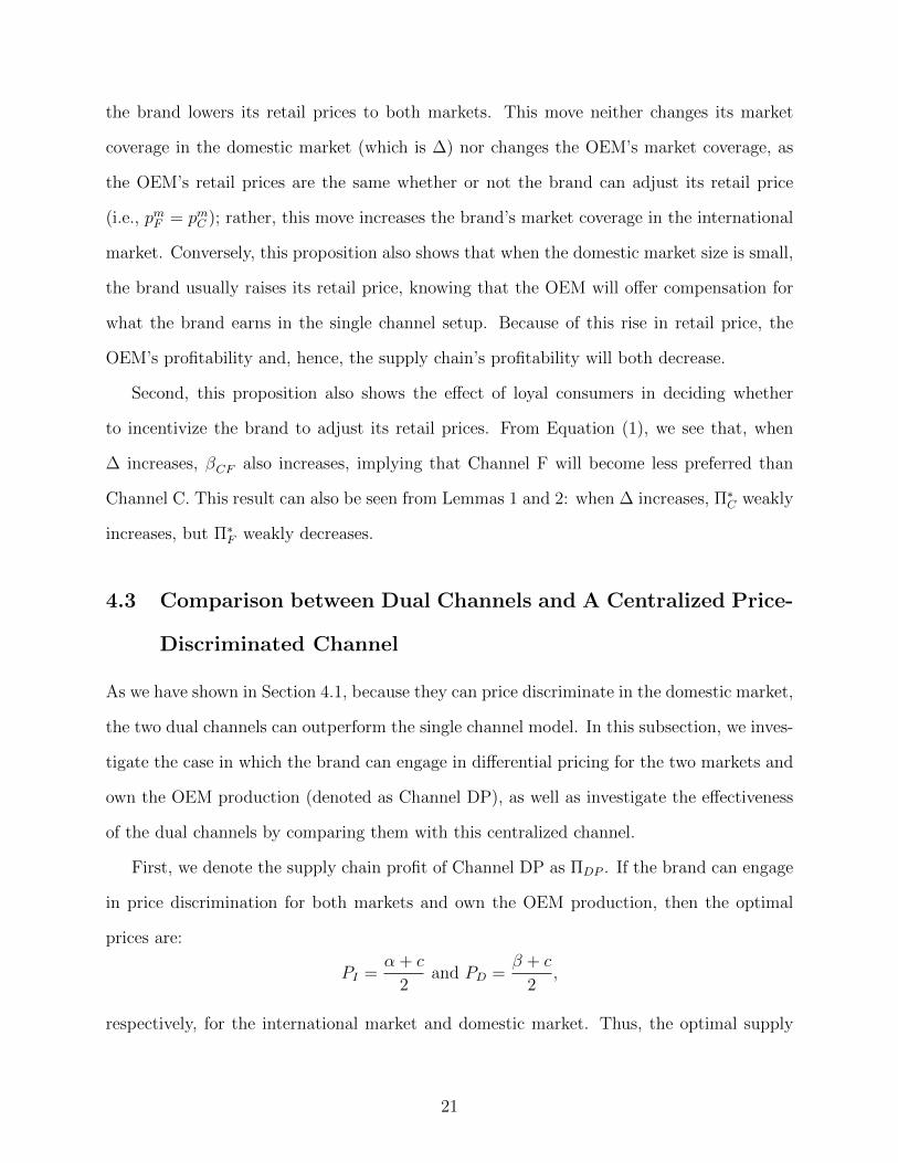
4.3 Comparison between Dual Channels and A Centralized Price-

Discriminated Channel

As we have shown in Section 4.1, because they can price discriminate in the domestic market,

the two dual channels can outperform the single channel model. In this subsection, we inves-

tigate the case in which the brand can engage in differential pricing for the two markets and

own the OEM production (denoted as Channel DP), as well as investigate the effectiveness

of the dual channels by comparing them with this centralized channel.

First, we denote the supply chain profit of Channel DP as ΠDP . If the brand can engage

in price discrimination for both markets and own the OEM production, then the optimal

prices are:

PI =α + c

2and PD =

β + c

2,

respectively, for the international market and domestic market. Thus, the optimal supply

21

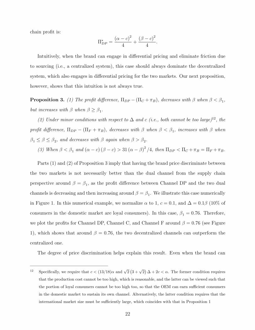
chain profit is:

Π∗DP =(α− c)2

4+

(β − c)2

4.

Intuitively, when the brand can engage in differential pricing and eliminate friction due

to sourcing (i.e., a centralized system), this case should always dominate the decentralized

system, which also engages in differential pricing for the two markets. Our next proposition,

however, shows that this intuition is not always true.

Proposition 3. (1) The profit difference, ΠDP − (ΠC +πB), decreases with β when β < β1,

but increases with β when β ≥ β1.

(2) Under minor conditions with respect to ∆ and c (i.e., both cannot be too large)12, the

profit difference, ΠDP − (ΠF + πB), decreases with β when β < β1, increases with β when

β1 ≤ β ≤ β2, and decreases with β again when β > β2.

(3) When β < β1 and (α− c) (β − c) > 31 (α− β)2 /4, then ΠDP < ΠC +πB = ΠF +πB.

Parts (1) and (2) of Proposition 3 imply that having the brand price discriminate between

the two markets is not necessarily better than the dual channel from the supply chain

perspective around β = β1, as the profit difference between Channel DP and the two dual

channels is decreasing and then increasing around β = β1. We illustrate this case numerically

in Figure 1. In this numerical example, we normalize α to 1, c = 0.1, and ∆ = 0.1β (10% of

consumers in the domestic market are loyal consumers). In this case, β1 = 0.76. Therefore,

we plot the profits for Channel DP, Channel C, and Channel F around β = 0.76 (see Figure

1), which shows that around β = 0.76, the two decentralized channels can outperform the

centralized one.

The degree of price discrimination helps explain this result. Even when the brand can

12 Specifically, we require that c < (13/18)α and√

2(3 +√

2)

∆ + 2c < α. The former condition requires

that the production cost cannot be too high, which is reasonable, and the latter can be viewed such that

the portion of loyal consumers cannot be too high too, so that the OEM can earn sufficient consumers

in the domestic market to sustain its own channel. Alternatively, the latter condition requires that the

international market size must be sufficiently large, which coincides with that in Proposition 1

22

Figure 1: Profit comparisons for Channel DP, Channel C, and Channel F

price discriminate between the two markets and eliminate the friction of sourcing, the OEM’s

second selling channel not only allows the supply chain to price discriminate between two

markets, but also allows the supply chain to charge two prices within the domestic market.

Therefore, a dual channel can be useful when the domestic market is of a particular size (i.e.,

when the brand can at most cover the loyal consumers using its retail price).

5 Extensions

In this section, we consider two extensions, relaxing assumptions to ensure that the robust-

ness of the insights derived from the base model are not challenged by these assumptions.

Specifically, in Section 5.1, we relax two assumptions of the negligible OEM retail cost and

OEM retail price by incorporating these two parameters in the OEM decision making pro-

cess. In Section 5.2, instead of assuming a group of loyal consumers and identical product

qualities regardless of selling channels, we consider quality difference between the brand and

OEM products, and allow consumers to choose the channel based on their utilities.

23

5.1 Additional Retail Cost and Price Constraint for OEM

We assumed in the previous section that the OEM does not incur any cost when it sells

product through its own selling channel. However, when compared to the brand that has

extensive experience in operating the brand’s selling channel, the OEM needs to incur a

higher retail cost in its channel; sometimes, this cost may impede the OEM from providing a

direct selling channel as a distribution outlet. To capture this effect, we normalize the brand

retail cost to zero, but model the OEM retail cost by a unit cost s ≥ 0. When s = 0, the

model is the same as in the previous sections.

Moreover, we have considered an OEM that can freely determine its own retail price

when it sells the product in the domestic market. This was the case for Galanz: the brand

microwave oven was priced from $1,000 to $3,000 RMB, but Galanz’s microwave often was

priced at only $300. That said, our model can be extended to other situations in which

the brand can influence the OEM’s pricing strategy. As one example, although the OEM

produces the product, it may demand use of the brand’s core technology. Therefore, the

brand can exercise its technology right to push the OEM to raise the product price. As

another example, the OEM can sell the brand products via its own channel; as the product

is still under the brand’s name, the brand can demand that the OEM maintains the price in

ways that help preserve brand image. For example, Foxconn launched its own e-commerce

platform–flnet.com–in China in 2015 to sell the products it manufactured, but these products

were still under the brand’s name (Luk 2015). We capture this situation by enforcing the

OEM to price the product that sells through the OEM channel to be L ∈ [0, 1] times larger

than the brand’s price.

Thus, in this section we consider the extension that incorporates the OEM retail cost, s,

and retail price constraint, L, and denote the channel as Channel LC if the brand does not

change its price after the launch of the OEM channel, and denote the channel as Channel LF

if the brand can change its price. In Channel LC, the OEM is subject to the price constraint

of LpB if pmC < LpB, whereas in Channel LF, the price is constrained by LpF if pmF < LpF .

24

We next show how relaxing these two assumptions affects the OEM’s channel strategy and

total production scale.

The following lemma characterizes the optimal prices for Channel LC and Channel LF,

respectively.

Lemma 4. For Channel LC, the optimal price is:

pmC =

(β−∆)+(c+s)

2, if β ≥ max{β1, βLC+};

LpB, if min{β1, βLC−} ≤ β < max{β1, βLC+};3α+3β+10c+8s

16, if β < min{β1, βLC−},

in which

βLC+ ≡3αL+ 4∆− 2c(2− L)− 4s

4− 3L, and βLC− ≡

2c(5− 2L)− 3α(2L− 1) + 8s

6L− 3.

For Channel LF, consider only the case where L > 1/2, the optimal price is:

pmF =

β−∆+c+s

2, if β > max{β2, βLF+};

LpF , if βLF− ≤ β ≤ max{β2, βLF+};

3α+3β+10c+8s16

, if β < βLF−,

in which

βLF+ =L(8∆ + 2

√2c+ 8α−

√2α) + 4∆− 4c− 4s

4 +√

2L,

βLF− =c+ s

2L− 1 + ∆, and

βLF− =

βLF−, if βLF− > β1;

min{β1, βLC−} if βLF− ≤ β1;.

Lemma 4 shows that the impact of the OEM retail price constraint will be effective only

when the domestic market is moderately sized. When the domestic market size is small, the

25

brand cannot charge a high price (as pC = pF = [3α+3β)+2c]/8), and hence the restriction

on the OEM retail price is not too strict. When the domestic market size is large, the OEM

will already charge a sufficiently high price. Therefore, only when the domestic market size

is moderate will the OEM pricing decision be affected. For Channel LF, we impose a minor,

sufficient condition on L: L > 1/2. Not only is this condition a sufficient one, but it also is

generally not very strict (i.e., asking the OEM to give less than 50% discount to the product).

Second, the impact of the OEM retail price constraint will be effective even when L is

as small as 1/2. To illustrate, let s = 0. For Channel LC to have a non-empty region, we

require that βLC− < β1 and βLC+ > β1. Substituting these threshold definitions into the two

inequalities, we obtain the necessary condition, L > (3α+3∆+7c)/(6α+6∆+4c), in which

the right-hand side is less than 1/2. Therefore, we assume that once this price constraint is

in effect, the OEM and supply chain profit will suffer. In turn, the total production scale

achieved from the OEM direct selling channel will also be harmed.

However, when we use the next proposition to compare the profits of the OEM, and hence

that of the supply chain, across Channels, B, LC, and LF, we show that for a reasonable

range of parameters on L, dual channels can still be useful, as long as the price constraint is

not too high.

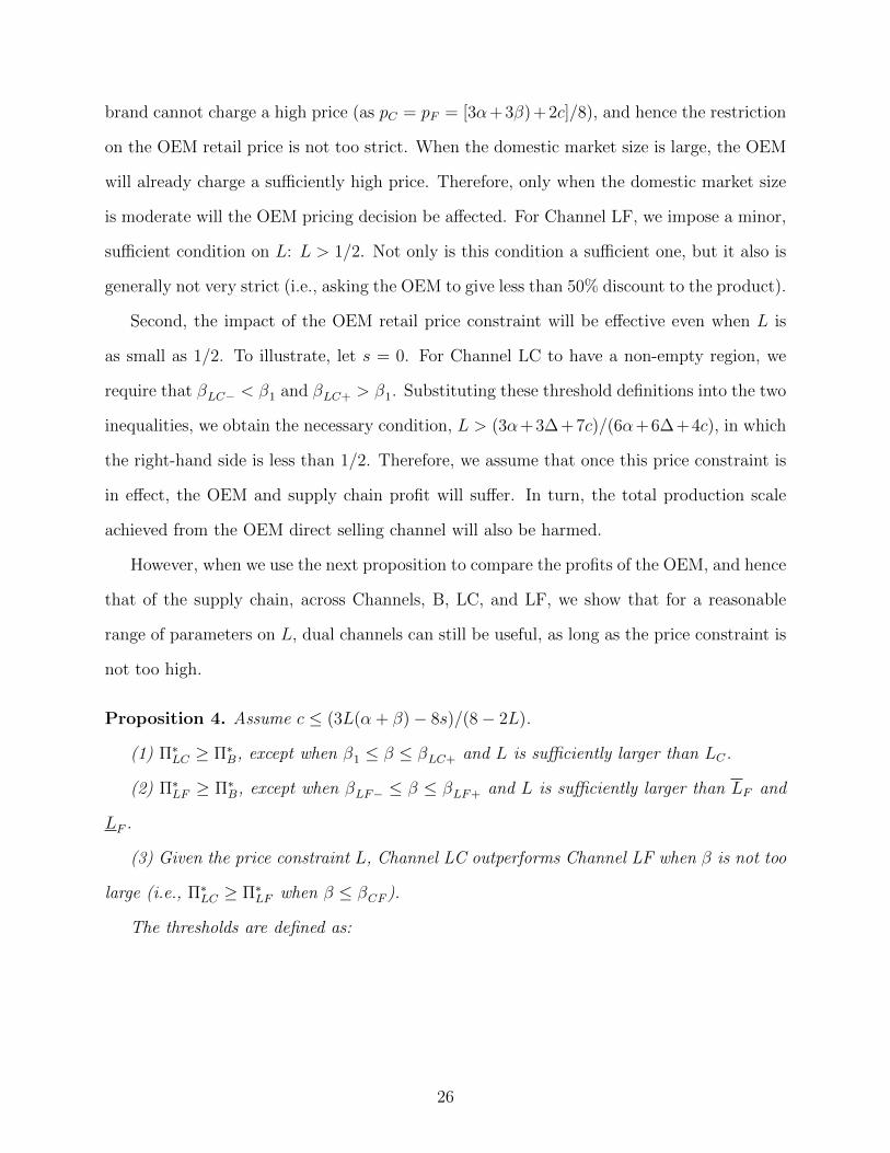
Proposition 4. Assume c ≤ (3L(α + β)− 8s)/(8− 2L).

(1) Π∗LC ≥ Π∗B, except when β1 ≤ β ≤ βLC+ and L is sufficiently larger than LC.

(2) Π∗LF ≥ Π∗B, except when βLF− ≤ β ≤ βLF+ and L is sufficiently larger than LF and

LF .

(3) Given the price constraint L, Channel LC outperforms Channel LF when β is not too

large (i.e., Π∗LC ≥ Π∗LF when β ≤ βCF ).

The thresholds are defined as:

26

LC = 4β −∆ + c+ s

3α + β + 2c,

LF = 4β −∆ + c+ s

(8− 1/√

2)α− 1/√

2β + 4∆ +√

2c, and

LF =β −∆ + c+ s

2β −∆.

Parts (1) and (2) of this proposition show that for a reasonable range of parameters on L,

the dual channels still outperform the single channel for both the OEM and the supply chain.

The profit difference of Π∗LC−Π∗B (Π∗LF −Π∗B) when β1 ≤ β ≤ βLC+ (βLF− ≤ β ≤ βLF+) is a

concave function of L, and the optimum occurs at L = LC (L = LF or L = LF ). Therefore,

there exists a threshold of L sufficiently higher than LC (min{LF , LF}), such that Π∗LC ≥ Π∗B

(Π∗LF ≥ Π∗B). Finally, Part (3) of this proposition shows that Π∗LC > Π∗LF if β < βCF , which

is the same threshold as in Proposition 2; this finding indicates that our insight on the choice

with respect to brand pricing remains.

To numerically show the range of L that will still yield similar insights to those in our

previous sections, we use the same setup in Section 4.3 and let s = 0.5 and c = 0.05. Figure

2 shows the profit comparisons between Channels B, LC, and LF, for L = 0.8 and L = 0.9.

We observe that, when L = 0.8, the two dual channels still outperform Channel B for any

valid β; however, when L = 0.9, the OEM profits that result from the dual channels can

be smaller than those that result from Channel B, when β is moderately sized. We have

tried other cases with s = 0 and s = c, and the results are qualitatively the same. Thus,

we conclude that although the additional retail cost and retail price constraint can reduce

the OEM’s incentive to operate a dual channel, our insight still remains for a wide range of

parameter sets.

5.2 Quality-embedded Utility Function

In our main model, we consider consumer preferences toward the brand’s selling channel

using loyal consumers (i.e., ∆), and assume identical product qualities, regardless of the

selling channels. Although in some markets, there exists consumers who will only purchase

27

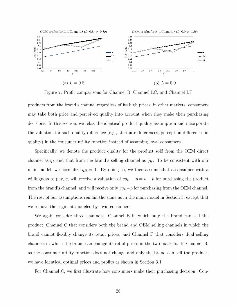
(a) L = 0.8 (b) L = 0.9

Figure 2: Profit comparisons for Channel B, Channel LC, and Channel LF

products from the brand’s channel regardless of its high prices, in other markets, consumers

may take both price and perceived quality into account when they make their purchasing

decisions. In this section, we relax the identical product quality assumption and incorporate

the valuation for such quality difference (e.g., attribute differences, perception differences in

quality) in the consumer utility function instead of assuming loyal consumers.

Specifically, we denote the product quality for the product sold from the OEM direct

channel as qL and that from the brand’s selling channel as qH . To be consistent with our

main model, we normalize qH = 1. By doing so, we then assume that a consumer with a

willingness to pay, v, will receive a valuation of vqH − p = v − p for purchasing the product

from the brand’s channel, and will receive only vqL−p for purchasing from the OEM channel.

The rest of our assumptions remain the same as in the main model in Section 3, except that

we remove the segment modeled by loyal consumers.

We again consider three channels: Channel B in which only the brand can sell the

product, Channel C that considers both the brand and OEM selling channels in which the

brand cannot flexibly change its retail prices, and Channel F that considers dual selling

channels in which the brand can change its retail prices in the two markets. In Channel B,

as the consumer utility function does not change and only the brand can sell the product,

we have identical optimal prices and profits as shown in Section 3.1.

For Channel C, we first illustrate how consumers make their purchasing decision. Con-

28

sumers will receive a value of zero if they do not purchase, receive a value of v − pB if

they purchase the product from the brand, and receive a value of vqL − pmC if they pur-

chase from the OEM channel. Comparing these utilities, we find that consumers with

v ≥ (pB − pmC )/(1− qL) will purchase from the brand, and pmC /qL ≤ v < (pB − pmC )/(1− qL)

will purchase from the OEM.13 For Channel F, we follow the same procedure and identify

that consumers with v ≥ (pF−pmF )/(1−qL) will purchase from the brand, whereas consumers

with pmF /qL ≤ v < (pF − pmF )/(1− qL) will purchase from the OEM.

With these market segments, we next find the optimal pricing strategies and the asso-

ciated profits (see the Appendix for the proof) and compare the profits between the dual

channels with Channel B (similar to Proposition 1), and compare the profits between the

two dual channels (similar to Proposition 2) in the following proposition.

Proposition 5. Using the quality-embedded utility function, we find that Π∗C = Π∗B, implying

that Channel C is reduced to Channel B, and Π∗F > Π∗B, implying that Channel F always

dominates Channels B and C.

This extension is useful in two ways. On the one hand, we still obtain a similar insight

that the dual channels weakly dominate the single channel even after we relax the assumption

of a fixed portion of loyal consumers to segmenting consumers by both product qualities and

prices. On the other hand, using this model setting, we find that the OEM dual channel can

strictly dominate the single channel only when the brand can flexibly adjust its retail price.

This is because, as in Channel C, the OEM needs to balance (1) the market size it can cover

in the domestic market due to the price and quality competition against the brand (which

13 To start, consumers with v ≥ max{PB , (pB − pmC )/(1 − qL)} will purchase from the OEM (i.e., their

willingness to pay is sufficiently large so that they will purchase the product, and their valuation of

purchasing from the brand channel is larger than that from the OEM channel). It is easy to show

that when pmC /qL < pB , we have PB < (pB − pmC )/(1 − qL). Moreover, when pmC /qL ≥ pB , then

PB > (pB − pmC )/(1 − qL) and thus, no consumers will purchase from the OEM; we do not consider

this trivial case, as it reduces to the single channel setting. Similarly, we can find the OEM’s market

coverage

29

limits its retail price range), (2) the wholesale price to the brand to offer sufficient incentives

(i.e., at least the same profit as before), and (3) a rigid brand’s pricing strategy. These three

tight constraints result in an optimal solution of not offering its own channel. That said, in

Channel F, the added lever from relaxing (3) enables the OEM to gain more profits, which

makes it profitable for the OEM to set up its own selling channel.

6 Conclusion

In this paper, we study the OEM’s dual channel strategy in a supply chain, in which the

OEM initiates its own channel and sells its product to the domestic market in addition

to having a brand selling channel. First, we take the single channel (Channel B) as the

benchmark and consider two dual channels, C and F. Whether or not the brand adjusts the

retail price due to the new channel, we find that retail prices set by the OEM in the domestic

market under both channels are the same; moreover, these retail prices are set downward, so

that the OEM is able to price discriminate and target relatively low-end consumers in the

domestic market. This outcome directly explains how Galanz used its ample capacity to offer

products to consumers in the Chinese market. Due to the effect of price discrimination, the

OEM can successfully incentivize the brand to allow for a dual channel, enhance the OEM

and supply chain profit, and greatly improve the OEM’s production scale. We further find

that when the domestic market is moderately sized, the two decentralized dual channels can

even outperform a centralized, price-discriminated single channel, as the two dual channels

allow for both price discrimination between the two markets and market segmentation within

the domestic market. Moreover, we extend our model to the case in which the OEM incurs

a retail cost, and the OEM retail price is subject to some constraint. Even with these

additional assumptions, our results are still robust, and all our managerial insights remain

the same for a wide range of parameter sets; that said, dual channels are less preferred by

the OEM, and thus by the entire supply chain, with this extension.

In addition, we analyze which type of dual channels the OEM prefers in the supply chain,

30

and find that the OEM always prefers the one with higher production scale. We find that

when the domestic market is mature enough (i.e., sufficiently large β), the OEM benefits

from a brand that can adjust the brand’s retail price freely and prefers Channel F. Knowing

the brand would adjust the retail price, the OEM’s best strategy, although contrary to our

initial intuition, is to reduce the wholesale price, leading to a lower retail price for the brand

as well as a higher production scale.

Our paper contributes to the operations and dual channel literature in the following ways.

First, we incorporate in our model the market structure and the OEM consideration of brand

reactions, including pricing and willingness concerns for a dual channel. Second, instead of

making a single market assumption and thus following the traditional dual channel literature,

we use a unique setting of the two separate markets, both international and domestic, to

capture OEMs in emerging countries fighting for both profit and scale growth. In this type of

situation, a dual channel may serve as an effective instrument to promote corporate growth

and create a win-win situation for OEMs that earn higher profit and production scale, for

brands that could extract some of the improved profits using a channel authorization fee,

and for consumers in emerging markets who can gain access to a lower-priced alternative

product. Finally, our model also highlights how OEMs can establish their direct selling

channel and offer incentives to influence their brand customers’ pricing practice. Given

different market structures, more flexible brand pricing may be preferred over constant brand

pricing practices.

Our work also offers practical values to OEMs. While China may lead the trend of

transitioning from an OEM to an OBM, the trade war between the US and China, the

rising labor costs in China, and gradually growing labor markets in southeast Asia and

Africa countries drive a redistribution of global supply chains. Those new OEMs emerging

from developing countries will need to consider their future growth and expansion. Our work

offers a guideline to these OEMs facing various market maturities (either their own operating

countries or their brand customers’ markets) with different brand pricing power (i.e., Channel

C or Channel F). Such a guideline is extremely valuable, as it is often challenging to balance

31

an OEM’s customer relationships with its brand building efforts (e.g., see Shih et al. 2010

for the transition of ASUS).

Although we completed a few extensions to ensure the robustness of our model insights,

there are several possibilities for future research that can enrich the understanding of how

OEMs may benefit/hurt themselves and their brand customers from establishing their own

selling channels. First, there could be a co-branding effect that benefits the OEM, thereby

enhancing economies of scale and lowering the sourcing costs for the brand. For example,

consumers who cannot afford a brand product may be attracted to the OEM product, as

they know that this OEM also produces the brand products that they like. This setting

can be further enriched when there are multiple brands and multiple OEMs. Second, as the

domestic market keeps increasing as the economy grows, the dynamics of such (potentially

stochastic) growth affects how consumers value a brand product. Taking the future growth

in mind, brands may face future challenges when they want to return to and exert marketing

efforts in domestic markets. How such stochastic growth changes the dynamics between the

OEM and the brand offers another interesting direction for future research.

References

Arya, A., B. Mittendorf, D. E. M. Sappington. 2007. The bright side of supplier encroach-

ment. Marketing Science 26(5) 651-659.

Berg, A., S. Hedrich, B. Russo. 2015. East Africa: The next hub for apparel sourcing? McK-

insey&Co article. https://www.mckinsey.com/industries/retail/our-insights/east-africa-

the-next-hub-for-apparel-sourcing

Cai, G. G. 2010. Channel selection and coordination in dual-channel supply chains. Journal

of Retailing 86(1) 22-36.

Caidieraro, F. 2016. The role of brand image and product characteristics on firms’ entry

and OEM decisions. Management Science 62(11) 3327-3350.

Cattani, K., W. Gilland, H.S. Heese, J. Swaminathan. 2006. Boiling frogs: pricing strategies

32

for a manufacturer adding a direct channel that competes with the traditional channel.

Production and Operations Management 15(1) 40-56.

Chen, J., L. Liang, D.-Q. Yao, S. Sun. 2017. Price and quality decisions in dual-channel

supply chains European Journal of Operational Research 259(3) 935-948.

Chiang, W.-Y.K. 2010. Product availability in competitive and cooperative dual-channel

distribution with stock-out based substitution. European Journal of Operational Research

200(1) 111-126.

Chiang, W.-Y.K., G. Chhajed, J.D. Hess. 2003. Direct marketing, indirect profits: A

strategic analysis of dual-channel supply-chain design. Management Science 49(1) 1-20.

Chiang, W.-Y.K., G.E. Monahan. 2005. Managing inventories in a two-echelon dual-channel

supply chain. European Journal of Operational Research 162(2) 325-341.

David, A., E. Adida. 2015. Competition and coordination in a two-channel supply chain.


Dodds, W. B., K.B. Monroe, D. Grewal. 1991. Effects of price, brand, and store information

on buyers’ product evaluations. Journal of marketing research 28(3) 307-319.

Dukes, A. J., E. Gal-Or, K. Srinivasan. 2006. Channel bargaining with retailer asymmetry.

Journal of Marketing Research 43(1) 84-97.

Dumrongsiri, A., M. Fan, A. Jain, K. Moinzadeh. 2008. A supply chain model with direct

and retail channels. European Journal of Operational Research 187(3) 691-718.

Grewal, D., R. Krishnan, J. Baker, N. Borin. 1998. The effect of store name, brand name and

price discounts on consumers’ evaluations and purchase intentions. Journal of retailing

74(3) 331-352.

Geng, Q., S. Mallik. 2007. Inventory competition and allocation in a multi-channel distri-

bution system. European Journal of Operational Research 182(2) 704-729.

Ha, A., X. Long, J. Nasiry. 2015. Quality in supply chain encroachment. Manufacturing

and Service Operations Management 18(2) 280-298.

Hua, G., S. Wang, T. C. E. Cheng. 2010. Price and lead time decisions in dual-channel

33

supply chains. European Journal of Operational Research 205 113-126.

Huang, W., J.M. Swaminathan. 2009. Introduction of a second channel: implications for

pricing and profits. European Journal of Operational Research 194(1) 258-79.

Iyer, G. 1998. Coordinating channels under price and non-price competition. Marketing

Science 17(4) 338-355.

Li, Z., S.M. Gilbert, G. Lai. 2014. Supplier encroachment under asymmetric information.

Management Science 60(2) 449-462.

Luk, L. 2015. Foxconn launches new E-commerce platform in China. Wall Street Journal

(March 4). http://www.wsj.com/articles/foxconn-launches-new-e-commerce-platform-in-

china-1425447691

Matsui, K. 2016. Asymmetric product distribution between symmetric manufacturers using

dual-channel supply chains. European Journal of Operational Research 248(2) 646–657.

Matsui, K. 2017. When should a manufacturer set its direct price and wholesale price in

dual-channel supply chains? European Journal of Operational Research 258(2) 501–511.

Matsui, K. 2020. Optimal bargaining timing of a wholesale price for a manufacturer with a

retailer in a dual-channel supply chain. European Journal of Operational Research 287(1)

225–236.

Modak, N. M., P. Kelle. 2019. Managing a dual-channel supply chain under price and

delivery-time dependent stochastic demand. European Journal of Operational Research

272(1) 147–161.

Mukhopadhyay, S. K. , X. Zhu, X. Yue. 2008. Optimal contract design for mixed channels

under information asymmetry. Production and Operations Management 17(6) 641-650.

Netessine, S., N. Rudi. 2006. Supply chain choice on the internet. Management Science

52(6) 844-864.

Ng, S.C.H., B. Li, X. Zhao, X. Xu, Y. Lei. 2010. Operations strategy at galanz. Richard

Ivey School of Business Case.

Rao, A. R., K.B. Monroe. 1989. The effect of price, brand name, and store name on buyers’

34

perceptions of product quality: An integrative review. Journal of marketing Research

26(3) 351-357.

Rodrıguez, B., G. Aydın. 2015. Pricing and assortment decisions for a manufacturer selling

through dual channels. European Journal of Operational Research 242(3) 901–909.

Shih, S. 1996. Me-Too is Not My Style: Challenge Difficulties, Break through Bottlenecks,

Create Values. The Acer Foundation.

Shih, W. C., H. H. Yu, H. C. Chiu. 2010. Transforming ASUSTek: Breaking from the Past.

Harvard Business School Case.

Tsay, A. A., N. Agrawal. 2004. Channel conflict and coordination in the e-commerce age.


Vinhas, A. S., J.B. Heide. 2014. Forms of competition and outcomes in dual distribution

channels: The distributor’s perspective. Marketing Science 34(1) 160-175.

Xiao, T., J. J. Shi. 2016. Pricing and supply priority in a dual-channel supply chain.

European Journal of Operational Research 254(3) 813–823.

Xiao, T., T.-M. Choi, T. C. E. Cheng. 2014. Product variety and channel structure strategy

for a retailer-Stackelberg supply chain. European Journal of Operational Research 233(1)

114–124.

Yan, Y., R. Zhao, T. Xing. 2019. Strategic introduction of the marketplace channel un-

der dual upstream disadvantages in sales efficiency and demand information. European

Journal of Operational Research 273(3) 968–982.

Yan, N., Y. Liu, X. Xu, X. He. 2020. Strategic dual-channel pricing games with e-retailer

finance. European Journal of Operational Research 283(1) 138–151.

Yang, Z., X. Hu, H. Gurnani, H. Guan. 2017. Multichannel distribution strategy: Selling to

a competing buyer with limited supplier capacity. Management Science 64(5) 2199-2218.

Yu, D. Z., T. Cheong, D. Sun. 2017. Impact of supply chain power and drop-shipping on a

manufacturer’s optimal distribution channel strategy. European Journal of Operational

Research 259(2) 554-563.

35

Appendix: Proofs and Table of Notations

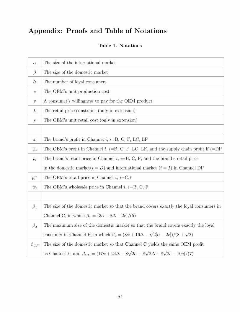
Table 1. Notations

α The size of the international market

β The size of the domestic market

∆ The number of loyal consumers

c The OEM’s unit production cost

v A consumer’s willingness to pay for the OEM product

L The retail price constraint (only in extension)

s The OEM’s unit retail cost (only in extension)

πi The brand’s profit in Channel i, i=B, C, F, LC, LF

Πi The OEM’s profit in Channel i, i=B, C, F, LC, LF, and the supply chain profit if i=DP

pi The brand’s retail price in Channel i, i=B, C, F, and the brand’s retail price

in the domestic market(i = D) and international market (i = I) in Channel DP

pmi The OEM’s retail price in Channel i, i=C,F

wi The OEM’s wholesale price in Channel i, i=B, C, F

β1 The size of the domestic market so that the brand covers exactly the loyal consumers in

Channel C, in which β1 = (3α + 8∆ + 2c)/(5)

β2 The maximum size of the domestic market so that the brand covers exactly the loyal

consumer in Channel F, in which β2 = (8α + 16∆−√

2[α− 2c])/(8 +√

2)

βCF The size of the domestic market so that Channel C yields the same OEM profit

as Channel F, and βCF = (17α + 24∆− 8√

2α− 8√

2∆ + 8√

2c− 10c)/(7)

A1

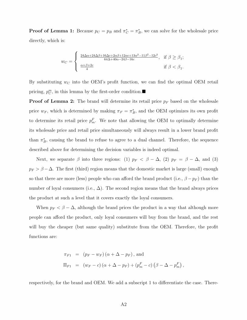
Proof of Lemma 1: Because pC = pB and π∗C = π∗B, we can solve for the wholesale price

directly, which is:

wC =

24∆α+24∆β+16∆c+2αβ+12αc+13α2−11β2−12c2

64∆+40α−24β−16c, if β ≥ β1;

α+β+2c4

if β < β1.

By substituting wC into the OEM’s profit function, we can find the optimal OEM retail

pricing, pmC , in this lemma by the first-order condition.�

Proof of Lemma 2: The brand will determine its retail price pF based on the wholesale

price wF , which is determined by making πF = π∗B, and the OEM optimizes its own profit

to determine its retail price pFm. We note that allowing the OEM to optimally determine

its wholesale price and retail price simultaneously will always result in a lower brand profit

than π∗B, causing the brand to refuse to agree to a dual channel. Therefore, the sequence

described above for determining the decision variables is indeed optimal.

Next, we separate β into three regions: (1) pF < β − ∆, (2) pF = β − ∆, and (3)

pF > β−∆. The first (third) region means that the domestic market is large (small) enough

so that there are more (less) people who can afford the brand product (i.e., β−pF ) than the

number of loyal consumers (i.e., ∆). The second region means that the brand always prices

the product at such a level that it covers exactly the loyal consumers.

When pF < β −∆, although the brand prices the product in a way that although more

people can afford the product, only loyal consumers will buy from the brand, and the rest

will buy the cheaper (but same quality) substitute from the OEM. Therefore, the profit

functions are:

πF1 = (pF − wF ) (α + ∆− pF ) , and

ΠF1 = (wF − c) (α + ∆− pF ) + (pFm − c)(β −∆− pFm

),

respectively, for the brand and OEM. We add a subscript 1 to differentiate the case. There-

A2

fore, following the aforementioned decision sequence, we can solve the optimum as:

pF =8α + 8∆−

√2[α + β − 2c]

8, and pFm =

β −∆ + c

2.

Finally, based on the value of pF , we can thus find the range of β that satisfies the condition,

pF < β −∆, which is β > β2 > β1.

In Case 3 when pF > β −∆, because the brand prices the product such that fewer than

∆ loyal consumers can afford the product, some of these loyal consumers must buy from the

OEM. Therefore, the profit functions become:

πF3 = (pF − wF ) (α + β − 2pF ) , and

ΠF3 = (wF − c) (α + β − 2pF ) + (pmF − c) (pF − pmF ) ,

respectively, for the brand and OEM. We add a subscript 3 to differentiate the case. There-

fore, following the aforementioned decision sequence, we can solve the optimum:

pF =3α + 3β + 2c

8= pB, and pFm =

3α + 3β + 10c

16.

Finally, based on the value of pF , we can thus find the range of β that satisfies the condition,

pF > β −∆, which is β < β1.

Finally, in Case 2, we consider pF = β −∆, and thus the range of β1 ≤ β ≤ β2. We add

a subscript 2 to differentiate the case. Because pF = β −∆, which is a fixed value, we can

easily find wF such that the brand’s profit will be the same as π∗B. Given the two values,

we thus can find the optimal OEM retail price pFm using the first-order condition, which is

pFm = (β −∆ + c)/2. �

Proof of Lemma 3: The results directly follow from Section 3.1, Lemmas 1 and 2 and the

first-order conditions. �

Proof of Proposition 1: First, we compare Channel B with Channel C. By substituting

A3

the optimal prices, we can obtain the optimal OEM profit of Channel C as:

Π∗C =

Π∗B + (3α−β+4∆−2c)2

64, if β ≥ β1;

2516

Π∗B, if β < β1.;,

which is always larger than Π∗B. Finally, Π∗C weakly increases with ∆, as can be seen directly

from the profit function.

Next, we compare Channel B with Channel F. We again separate β into three regions:

(1) β < β1, (2) β1 ≤ β ≤ β2, and (3) β > β2. By substituting the optimal prices in Lemma

2, we can find the optimal profits in each region.

When β < β1, the optimal profit is Π∗F3 = Π∗C , which is always higher than the profit in

Channel B. When β > β2, the optimal profit is:

Π∗F1 = Π∗B +

√2(α + β)(α + ∆) + 2(β −∆)2 − (α + β)2

32

+c[(4− 2

√2)(α + ∆)−

√2(α + β)] + (2

√2− 2)c2

8.

If the sum of the latter two terms is positive, then Π∗F1 > Π∗B, which indicates that a

dual channel effectively improves the OEM profit. To prove this, we start with the profit

difference, Π∗F1−Π∗B, which is obviously a convex function. Thus, we can use the first-order

condition to find its minimum:

β∗ =∆(4−

√2) + α(2−

√2) +

√2c

2.

However, because β2 > β∗, we obtain:

β2 − β∗ =

√2(4 +

√2)(α + ∆− c)

16 + 2√

2> 0.

A4

Given the feasible range of β(> β2), the minimum of Π∗F1−Π∗B happens at β = β2, which is:

Π∗F1 − Π∗B =(48√

2− 64 + 9c)((α + ∆)− c)2

(16 + 2√

2)2> 0.

Therefore, we can conclude that Π∗F1 will always outperform Π∗B.

Finally, when β1 ≤ β ≤ β2, the optimal profit is:

Π∗F2 = Π∗B +−56∆2 − 32α∆ + 80β∆− 3α2 + 26αβ − 27β2 + 4c(7β − 5α− 12∆)− 4c2

32.

First, we find that the numerator of Π∗F2 − Π∗B is a concave function of β, and hence the

minimum happens on the two boundaries:

β =3α + 8∆ + 2c

5or

8α + 16∆−√

2(α− 2c)

8 +√

2.

Therefore, if we can find that the value is higher than 0 on both boundaries, then Π∗F2 > Π∗B.

By substituting β = β1 into Π∗F2 − Π∗B, the numerator becomes (72/25)(α + ∆ − c)2 > 0.

By substituting β = β2, we have 16(24√

2 − 23)(α + ∆ − c)2/(8 +√

2)2 > 0. As a result,

Π∗F2 > Π∗B. Together with the previous two cases, we obtain that Π∗F ≥ Π∗B.

Finally, we discuss the profit functions in the three regions with respect to the number

of loyal consumers. Because β > β2 (used in the first inequality), we find that:

∂Π∗F1

∂∆=

√2(α + β)− 4(β −∆) + 4c(4− 2

√2)

32<−(8− 5

√2)

(α + ∆) +(29− 14

√2)c

8(8 +√

2) ,

which will be negative if α is large:

α >(24− 7

√2)(∆− c)

9√

2− 8.

Next, because β1 ≤ β ≤ β2, we find that ∂Π∗F2/∂∆ increases with β. Thus, the upper bound

A5

of this first derivative happens at β = β2:

−(24− 7

√2)c+

(9√

2− 8)α−

(24− 7

√2)

∆

2(8 +√

2) ,

which is negative if α is large:

α >(29− 14

√2)c

8− 5√

2−∆.

Finally, because β < β1, Π∗F3 is independent of ∆.�

Proof of Proposition 2: Using Lemmas 1 and 2, we prove this part by separating the

domestic market size, β, into three regions: (1) β < β1, (2) β1 ≤ β ≤ β2, and (3) β > β2.

When β < β1, as pF is the same as pB, which is the same as pC , and pmF = pmC , the two dual

channels are the same.

When β1 ≤ β ≤ β2, the profit difference between the two is:

Π∗C − Π∗F2 =[3α− 5β + 8∆ + 2c][5α− 11β + 16∆ + 6c]

64> 0,

as β > β1 implies that 3α− 5β + 8∆ + 2c > 0 and 5α− 11β + 16∆ + 6c > 0.

When β ≥ β2, the profit difference becomes:

Π∗F1 − Π∗C =(α + β − 2c)(10c− 24∆− 8

√2c− 17α + 8

√2∆ + 8

√2α)

64.

As α+ β > 2c, when β > βCF , then ΠF1 > ΠC . This threshold is higher than β2, such that:

βCF − β2 =8(8− 5

√2)((α + ∆)− c)

56 + 7√

2> 0.

Moreover, in this region where β > βCF , pF < pC . This is because (1) pC increases with

A6

β whereas pF decreases with β, and (2) when β = βCF , the two are the same:

pC |β=βCF=

(9− 3√

2)(α + ∆) + c(3√

2− 2)

7= pF |β=βCF

.

As a result, when β ≤ β1, pF is the same as pB; when β1 < β ≤ β2, pF increases faster than

pC , and thus pC < pF in this region; when β2 < β < βCF , pC increases with β whereas pF

decreases with β, and pC < pF ; and finally, when β > βCF , pF < pC , and this result leads

to the second half of the proof. �

Proof of Proposition 3: When β < β1, the supply chain profit difference is:

Π∗DP − (Π∗C + π∗B) = Π∗DP − (Π∗F3 + π∗B) =31 (α− β)2 − 4 (α− c) (β − c)

256.

As β increases, the difference decreases (the first derivative is negative), indicating that when

β increases (but is still smaller than α), we obtain Π∗C + π∗B = Π∗F3 + π∗B > Π∗DS. This result

shows that having the brand price discriminate is not necessarily better than the dual channel

offering from a supply chain perspective. Specifically, when (α− c) (β − c) > 31 (α− β)2 /4,

then Channels C and F can achieve a higher profit than Channel DP.

However, for Channel C, when β ≥ β1, we obtain:

Π∗DP − (Π∗C + π∗B) =α2 + 9β2 − 6αβ + 8β∆− 24α∆− 16∆2 + 4c(4∆ + 7α + 3β) + 8c2

64,

which increases with β, as the numerator of its first derivative is (18β − 6α+ 8∆) + 12c > 0

because β > β1 > 1/3α. On the other hand, for Channel F, when β1 ≤ β ≤ β2, we obtain:

Π∗DP−(Π∗F2 + π∗B) =(56∆2 + 32α∆− 80β∆ + 8α2 − 32αβ + 31β2)− 16c(2β − α− 3∆) + 16c2

32,

which is an increasing function of β, as the numerator of the first derivative is (−80∆ −

32α+ 62β)− 32c, which is positive because β > β1. That is, as long as c < (13/18)α (which

A7

is often true, as there would otherwise not be much profit left for production), then:

−80∆− 32α + 62β − 32c >2

5[13α + 48∆− 18c] > 0.

When β > β2, however, we find an opposite direction, such that:

Π∗DP − (Π∗F1 + π∗B) =[(9− 4

√2)α2 + β2 − 4

√2∆α +

(2− 4

√2)αβ +

(16− 4

√2)β∆− 8∆2]

32

+4c[(3

√2− 6)α + (2

√2− 4)∆ + (

√2− 1)β)] +

(8√

2 + 12)c2

32,

which is a decreasing function of β when ∆ and c are not too high (i.e.,√

2(3 +√

2)

∆+2c <

α), as the numerator of its first derivative is:

[β −(2√

2− 1)α +

(8− 2

√2)

∆] + 4(√

2− 1)c

16<

[−α +√

2(3 +√

2)

∆] + 2c

8(√

2 + 1) ,

thus completing the proof.�

Proof of Lemma 4: We first start with Channel LC by considering the two regions of β

as shown in Lemma 1: (1) β ≥ β1 and (2) β < β1. When β ≥ β1, if there is no constraint

on the OEM retail price, the optimal price will be:

pmC =β −∆ + (c+ s)

2. (A1)

Therefore, if β ≤ βLC+, then pmC < LpB, and hence the OEM must set its price at LpB.

When β < β1, if there is no OEM retail price constraint, the optimal price becomes:

pmC =10c+ 3α + 3β + 8s

16. (A2)

Therefore, if β ≥ βLC−, the OEM must set its price at LpB.

Next, we discuss Channel LF using a similar procedure. Similar to the proof of Lemma

2, we consider three regions: (1) β2 < β, (2) β1 ≤ β ≤ β2, and (3) β < β1. When β2 < β,

A8

the unconstrained OEM price is the same as (A1); however, when β ≤ βLF+, then the price

is affected. When β1 ≤ β ≤ β2, the unconstrained OEM price is again the same as in (A1),

but pF has changed to β −∆. By using simple algebra, we find that only when β ≥ βLF− is

the OEM retail price affected by L. Finally, when β < β1, the unconstrained OEM price is

the same as in (A2). As a result, we can find that if β ≥ βLC−, then the OEM retail price

is affected.

Finally, we need to show that when βLF− > β1, then βLC− > β1. Otherwise, a dis-

continuity of affected regions may exist (i.e., when β1 < βLF− < β ≤ max{βLF+, β2} and

βLC− < β < β1, the OEM retail price is affected). The condition, βLF− > β1 implies that:

s >(3α + 8∆)(2L− 1) + ∆(3α + 8∆)− c(7− 4L− 2∆)

5.

With this condition and L > 1/2, we substitute:

βLC− − β1 =2c(5− 2L)− 3α(2L− 1) + 8s

6L− 3)− 3α + 8∆ + 2c

5

>∆(3α + 8∆) + 40∆(2L− 1) + c(49− 28L+ 2∆)

30L− 15)> 0.�

Proof of Proposition 4: (1) As shown in Proposition 1, when the price constraint does

not affect the OEM profit, Π∗LC = Π∗C ≥ Π∗B. Therefore, we only need to consider the two

regions that will be affected: β1 ≤ β ≤ βLC+ and βLC− ≤ β < β1. By substituting the

pricing decisions into the OEM profit, we obtain:

Π∗LC =

Π∗B + A, if β1 ≤ β ≤ βLC+;

Π∗LC2, if βLC− ≤ β < β1;,

A9

in which

A =(1− L)(3(α + β) + 2c)[3α− 5β + 8∆ + 3L(α + β)− 2c(3− L)]

64

+s(∆− β) +sL(2c+ 3α + 3β)

8, and

Π∗LC2 = Π∗B + (LpB − c− s)(1− L)pB.

For β1 ≤ β ≤ βLC+, Π∗LC −Π∗B = A is a concave function of L, and the optimal happens

at L = LC = 4(β − ∆ + c + s)/(2c + 3α + 3β). Moreover, for the region β1 ≤ β ≤ βLC+

to even exist, we also need L > LC . As a result, A only decreases with L in the region of

feasible β. Therefore, there exists a threshold of L such that Π∗LC > Π∗B, only when L is

higher than the threshold.

For βLC− ≤ β < β1, since 0 ≤ L ≤ 1, if c < (3L(α + β) − 8s)/(8 − 2L), we obtain

(Lp∗B − c− s)(1− L)(pB) ≥ 0, and thus Π∗LC2 ≥ Π∗B.

(2) Similarly, we only need to consider the three regions that will be affected:

Π∗LF =

Π∗B + AF1, if β2 ≤ β ≤ βLF+;

Π∗B + AF2, if βLF− ≤ β < β2;

Π∗LC2, if βLC− ≤ β < β1;

,

in which

AF1 =[8(c+ s+ ∆) +

√2L(β − c)− 8Lα][8(∆− β + ∆L) + 2

√2Lc+ 8Lα +

√2L(β − α)]

64

−(α− 2c+ β)2

16− (√

2(α− 2c+ β))(4c− 4∆− 2√

2c− 4α +√α +√

2β)

32, and

AF2 = (α− β + 2∆)

[(β −∆)− c− (α− 2c+ β)2

32(2∆ + α− β)

]+(β −∆)(1− L)(L(β −∆)− (c+ s))− (α + β − 2c)2

16.

When β2 < β ≤ βLF+, we will prove that the profit difference, Π∗LF1 − Π∗B, decreases

with L, and hence there exists a threshold that Π∗LF1 = Π∗B. First, the condition β ≤ βLF+

A10

requires that L ≥ LF . For L in this range, we know that Π∗LF − Π∗B = AF1 decreases with

L, as AF1 is a concave function of L, and the optimal solution happens at L = LF . From

Proposition 1, we know that Π∗LF ≥ Π∗B at L = LF (as in this case, the constraint L yields

the same profit as the case without the constraint), and hence when L is sufficiently small,

Π∗LF ≥ Π∗B.

When βLF− ≤ β ≤ β2, we follow the same procedure. The condition, β ≥ βLF−,

will be satisfied only when L ≥ LF . In this case, we can obtain the concave property of

Π∗LF −Π∗B = AF2, and the first-order condition that implies the optimal solution at L = LF

together show that Π∗LF − Π∗B decreases with L. Therefore, there exists a threshold that

Π∗LF ≥ Π∗B.

Finally, when βLC− ≤ β < β1, Channel LF degenerates to Channel LC, which we previ-

ously proved.

(3) To prove the result, we consider three cases: β2 < β, β1 ≤ β ≤ β2, and β < β1.For

simplicity’s sake, we denote cases similar to the ones in the proofs of Lemmas 1 and 2, and

add L for the price constrained case. For the last case, when β < β1, Channel F and LF

degenerated to C and LC, respectively, and hence Π∗LC = Π∗LF .

When β2 < β, three scenarios can happen: (i) C1 compares with F1, (ii) LC1 compares

with LF1, and (iii) C1 compares with LF1. As LC > LF , the F1 and LC1 will not coexist.

For (i), we have proved it in Proposition 2, for when β < βCF , Π∗LC ≥ Π∗LF . For (iii), since

the cases without the constraint L are always better than the cases with L (i.e., Π∗F1 ≥ Π∗LF1)

and from (i) above that Π∗C1 > Π∗F1 if β < βCF , we obtain that Π∗C1 > Π∗F1 ≥ Π∗LF1 when

β < βCF . For (ii), we discuss it using Proposition 2. When β < βCF , pC < pF , and

hence when there is a price constraint, it will affect Case LF1 more than LC1, and hence

Π∗LC1 ≥ Π∗LF1, regardless of the value of L.

When β1 ≤ β ≤ β2, we consider three scenarios: (i) C1 compares with F2, (ii) LC1

compares with LF2, and (iii) C1 compares with LF2, as LC > LF (because β > β1), Case

F2 and Case LC1 will not coexist. For (i) and (iii), Π∗C ≥ Π∗F always holds. For (ii), the

A11

profit difference is:

Π∗LC1 − Π∗LF2

=(3α + 8∆− 5β + 2c)[(β −∆)(8L− 11L2 − 11) + (5− 3L2)(α + ∆) + 2c(4L− L2 + 3) + 8Ls]

64.

Because β ≥ β1, 3α + 8∆ − 5β + 2c ≥ 0. To prove the second term of the numerator is

non-negative, we note that this term decreases in β and when β = βLC+ (the upper bound

where Π∗LC = Π∗LC1), this term is positive, which allows us to conclude that Π∗LC1 ≥ Π∗LF2.�

Proof of Proposition 5: We start with Channel C. Following the segments in Section 5.2,

we can express the profit functions for the two parties as:

πC = (pB − wC)

(α + β − pB −

pB − pmC1− ql

),

ΠC = (wC − c)(α + β − pB −

pB − pmC1− ql

)+ (pmC − c)

(pB − pmC1− ql

− pmCql

).

As wC is set so that πC = π∗B, we then can substitute wC into ΠC , which is reduced to:

ΠC = Π∗B + (PB − c)(pB −

pB − pmC1− ql

)+ (pmC − c)

(pB − pmC1− ql

− pmCql

).

As the profit function is concave in pmC , the the OEM’s optimal retail price satisfies the

first-order condition if pB < (pB − pmC )/(1 − ql) at the first-order solution, and satisfies

pB = (pB − pmC )/(1 − ql) (or equivalently, pmC = pBql), otherwise. We know that the first-

order condition yields the following solution:

pmC =3ql(α + β) + 4c− 2cql

8,

but it is obvious that this pmC does not satisfy the condition, which means we then have

pmC = pBql. In other words, although we consider a dual channel, it is optimal for the OEM

not to operate its own selling channel, as it will not cover any of the consumers in the

A12

domestic market, and we thus have Π∗C = Π∗B

We follow a similar procedure for Channel F. Given the segments identified in Section

5.2, we can formulate the two parties’ profit functions as:

πF = (pF − wF ) ∗(α + β − pF −

pF − pmF1− ql

)ΠF = (wF − c) ∗

(α + β − pF −

pF − pmF1− ql

)+ (pmF − c) ∗

(pF − pmF1− ql

− pmFql

)

The brand’s optimal retail price, a function of wF and pmF , can be derived from the first-order

condition of ∂πF/∂pF = 0. The OEM’s wholesale price, wF to the brand is maintained at

the level so that πF = π∗B. Substituting the two into ΠF , we thus have a concave function

of ΠF with respect to pmF . As a result, solving the first-order condition that ∂ΠF/∂pmF = 0,

we then have the following optimal price:

pmF =αql + βql + 2c

4.

We note that this solution will not violate the constraint that pF < (pF − pmF )/(1− ql), and

hence, this solution is indeed optimal.

By substituting this optimal price back into the profit function to obtain Π∗F , we next

prove that Π∗F > Π∗B using the following steps. First, it is easy to show that ∂2(Π∗F −

Π∗B)/∂c2 > 0 for all positive c, and ∂(Π∗F − Π∗B)/∂c > 0 and Π∗F > Π∗B at c = 0. The former

condition shows that Π∗F increases faster than Π∗B for c ≥ 0, and the later conditions show

that even when c is 0, Π∗F > Π∗B. Combining these two together, we conclude that Π∗F > Π∗B

for all feasible c ≥ 0. �

A13

Channel Design and OEM Growth in a Multi-market Setup

Documents

Transcript of Channel Design and OEM Growth in a Multi-market Setup