Changes in seasonal patterns - European University...

Journal of Economic Dynamics and Control 18 (1994) 1143- 1171. North-Holland

Changes in seasonal patterns

Are they cyclical?*

Fabio Canova Brown University, Providence, RI 02912, USA

Eric Ghysels Universith de Montrtal, Monmkzl. Q&. H3C 3J7, Canada

Received July 1992, final version received May 1993

This paper explores the hypothesis that the seasonal patterns of macroeconomic variables vary with expansions and contractions. Graphical techniques and generalized predictive tests for structural stability are used to identify and test patterns of changing seasonality. A Monte Carlo exercise shows the power of the tests against interesting alternatives. The empirical results suggest that seasonal patterns are unstable and that in many cases changes are linked to the stages of the business cycle. The forecasting costs incurred by treating seasonality as constant are discussed and evaluated.

Key words: Seasonality; Business cycles; Structural stability

JEL cIassiJ?cation: ClO; C12; C22; E32

1. Introduction

It is typical in the macroeconomics literature to neglect seasonal fluctuations either by constructing theoretical models which abstract from the seasonal

Correspondence IO: Eric Ghysels, Departement de Sciences Economiques, Universite de Montreal, P.O. Box 6128, Station A, Montreal, Que. H3C 357, Canada.

*The first author thanks for the financial support of the European University Institute Research Fund and the second for the financial support of SSHRC and NSERC of Canada as well as the Fonds FCAR of Quebec. Part of this work was completed while the second author was a Visiting Research Fellow at the Cowles Foundation, Yale University. Its hospitality and financial support are also gratefully acknowledged. We would,also like to thank Herman Van Dijk, Philip Franses, Neil Shepard, and two anonymous referees for their comments and suggestions, and Gregory Hess of the Monetary Section of the Board of Governors of the Federal Reserve Board for his invaluable help in supplying us with data and graphs.

0165-1889/94/$07.00 0 1994-Elsevier Science B.V. All rights reserved

1144 F. Canova and E. Ghysels, Changes in seasonal patterns

component or by using seasonally adjusted data both in testing theories and in analyzing policy issues. Those studies that explicitly examine the information contained in the seasonal component of time series generally assume that deterministic dummies capture the most interesting aspects of these fluctuations [see, e.g., Miron (1986) or Singleton (1988)].

The statistical modelling of seasonal fluctuations with dummies has gained widespread acceptance in macroeconomics for four reasons. First, it is a simple and easily reproduced procedure which can be mechanically applied to any time series, therefore reducing judgmental decisions on the possible forms seasonality can take. Second, for most series, seasonal dummies capture a substantial portion of the existing seasonal fluctuations. Third, the procedure implements a traditional statistical view that the business and seasonal cycles are phenomena to be studied separately. Finally, the application of dummies to seasonally unadjusted series generates seasonal facts which correspond to econom- ists’ prior notion of seasonal fluctuations [see, e.g., Barsky and Miron (1989)].

Despite its widespread use, the dummy approach to seasonality neglects two important facts. First, the traditional separation of seasonal and business cycles is not an attribute of modern dynamic business cycle theory which, in general, embodies extensive cross-frequency restrictions [see, e.g., Ghysels (1988)] and, in many cases, contains explicit information about the interaction of seasonal and business cycles [see, e.g., Hansen and Sargent (1992)]. Second, a number of researchers have noted that the seasonal patterns of many macroeconomic variables appear to evolve over time [see, e.g., Bell and Hillmer (1984)] and several statistical tests have been suggested to formally examine whether seasonal patterns are constant (stable) or not [see, e.g., Franzini and Harvey (1983), Canova and Hansen (1991), Sutradhar, MacNeill, and Dagum (1991)].

When seasonals drift through time a simple deterministic seasonal dummy model should be abandoned in favor of a model which also contains some stochastic elements. One possible specification for stochastic seasonality is a model with seasonal unit roots as in Dickey, Hasza, and Fuller (1984) or Hylleberg, Engle, Granger, and Yoo (HEGY) (1990). A standard justification for using such a model is that changes in the seasonal patterns are long-run phenomena primarily linked to modifications of institutional factors of the economy. While institutional modifications certainly are contributing elements to the changes we observe, short-run factors may also play a significant role. For example, Ghysels (1990) suggests that changes in the seasonal patterns of several post-WWII aggregate quarterly US time series may be linked to the stages of the business cycle. There are two implications of this finding. First, both time series models which represent seasonal factors with deterministic dummies (no-change model) and those with seasonal unit roots (long-run changes) are subject to specification errors. Second, because standard tests for unit roots at seasonal frequencies are perversely affected by the presence of seasonal mean shifts in the same way as standard unit root tests are affected by the presence of infrequent

F. Canova and E. Ghysels. Changes in seasonal palterns 1145

breaks in the long-run properties of the data [see, e.g., Perron (1990)], recent findings suggesting the existence of seasonal unit roots may be erroneous.

The idea to link the seasonal shifts to the business cycle was motivated by the fact that dynamic macroeconomic models imply a nontrivial interaction between the seasonal component and other types of fluctuations. Ghysels studied this interaction using a model where seasonal dummies were allowed to differ in expansions and recessions. The evidence presented, while indicative of the complex interactions contained in the data, was not conclusive since it was based on a simple model with the NBER business cycle chronology as the basis for the switching regime indicator function.

The purpose of this paper is to study in detail the existence of medium-run changes in seasonal patterns for a large class of quarterly aggregated and monthly disaggregated US time series. In our analysis we rely on both informal graphical methods [as suggested, e.g., by Franses (1991)] and on generalized predictive tests (GPT) for structural stability [as proposed by Dufour, Ghysels, and Hall (DGH) (1991)]. The hypothesis of interest here is one where we allow for the presence of multiple breaks at unknown dates under the alternative. Because GPT are exploratory and can detect single or multiple shifts that are either temporary or permanent in nature, they are, in principle, better suited than alternative stability tests to examine the presence of cyclical variations in seasonal patterns. A relevant question is whether in practice they can detect breaks in processes which switch state recurrently over time. Using a small Monte Carlo design we show that the tests have good power against the type of alternatives we are most interested.

The empirical analysis shows that the majority of the US aggregate data we examined possess seasonals which drift over time and that, in some cases, these changes are linked to the stages of the business cycle. One special case which deserves mention is the Ml series which, in addition to cyclical instability, displays a puzzling second-quarter upward trend. The evidence for disaggregated data is statistically less significant but economically more compelling because changes emerge primarily during recessions.

We attempt to quantify the gains one can obtain by allowing seasonals to evolve over time with a simple forecasting exercise. We show that both a model which conditions the seasonal switches on business cycle phases, and a flexible Bayesian model, which allows the coefficients of the dummies to drift over time, improve upon a model where seasonals are treated as constant. For the second specification and for most series, the average forecasting gain at each step is about 10%.

The rest of the paper is organized as follows. Section 2 documents the features of seasonal patterns and their variation through time. In section 3 we review the statistical tests, describe the modifications needed to adapt them to our context, and perform a small Monte Carlo experiment to check the power of the tests against some interesting alternatives. The empirical analysis is contained in

1146 F. Canova and E. Ghysels. Changes in seasonal patterns

section 4. Section 5 discusses the costs of treating seasonality as constant, and section 6 concludes the paper.

2. The evolution of seasonal patterns

In this section we employ a simple graphical technique [also used, for instance, by Franses (1991) and Hylleberg, Jorgensen and Sorensen (1991)] to highlight a possible relationship between the evolution of seasonal patterns and the phases of the business cycle. We limit our attention to quarterly time series since graphical methods are cumbersome to read and interpret with monthly data. Although the graphical technique does not require stationarity assump-

tions, the graph are easier to interpret if the long-run features of the series are filtered out. For this purpose we first-differenced the log of the series. While other transformations are possible, the evidence we present is essentially independent of the exact stationary inducing transformation employed. Intuitively, this occurs because although alternative detrending methods affect business cycle frequencies differently, they appear to have little impact on the seasonal frequencies of the spectrum and on the cross-spectrum of the components [see Canova (1992)].

In what follows we denote with {yin} all observations pertaining to quarter i= l,... ,4, where n is a yearly sampling index, and plot {yr,, . . . ,yan} on one graph. Given our stationary inducing transformation, the plots can be used as specification diagnostics for the process generating seasonal patterns. For example, if the data generating process is one of stationary mean shifts for each quarter around a log first-differenced process, the graphs should display stationary plots. If the data generating process is one of deterministic mean shifts for each quarter, the graphs should display completely parallel lines. Finally, if the plots of the four quarters drift apart or cross, the quarterly processes is not stationary around a particular (seasonal) mean. One typical example of such a class of time series is a seasonal unjt root process whose quarterly plots will display some crossing over time, i.e., summer becomes winter.

To highlight a possible relationship between the pattern of seasonal instabili-

ties and phases of the business cycle, we shade recession years according to the NBER business cycle chronology. Since the chronology is monthly, we convert it to a quarterly series using a ‘majority rule’ [as in Ghysels (1991b)], i.e., if at least two months of the quarter are in an expansion (contraction), the quarter is classified as an expansion (contraction). Shaded areas on the graphs represent years where at least one quarter is in a recession.

Fig. 1 graphs the evolution of seasonal patterns of six US quarterly time series [GNP, Fix Investments (IFIX), Consumption of Durables (CDUR), Ml, Em- ployment (EMPL), and Final Sales (FINSALE)] and their relationship with the business cycle. All series but FINSALE are in log first-difference.

F. Canova and E. Ghysels, Changes in seasonal patterns 1147

!

Fig. 1. Annual plots of quarterly data.

In all six graphs there appears to be visual support for the idea that he magnitude and the evolution of seasonal fluctuations are sensitive to the various stages of the business cycle. Concentrating on the evidence emerging from 1970 on, the plot of IFZX indicates a tendency for the four quarterly time series to converge in recessions and to diverge in expansions suggesting that for this variable seasonal and cyclical components interact multiplicatively. The plot of


CDUR shows parallel movements of the four quarters over the cycle: in expansions all quarters shift up and in recessions all quarters shift down, suggesting the presence of a cyclical level effect. This pattern emerges to a lesser extent also in GNP, and FZNSALE, where the first quarters (the lowest time series in each plot) seem to move in the opposite direction of the other three quarters over the cycle. The quarterly structure of EMPL is more complicated. Early in the sample the four time series roughly follow the four quarters of GNP. Over the last ten years a seasonal inversion tends to appear.

The most striking features, however, emerge with the Ml series whose second quarter (the solid line) displays a clear upward trend of about 3% throughout the entire sample, apart from a small decline right after WWII and a sharp dip at the beginning of the 1980’s when the Fed targeted monetary aggregates. Fig. 2 highlights these features by plotting the time series for each quarter separately around its mean.

One possible explanation for this pattern is that income taxes in the US are paid in the second quarter and income taxes have become an increasing proportion of income over the last thirty years. In this case, the money demand function of agents is not only seasonal, but may also display a trend in the second quarter. But while the presence of this upward trend in the second quarter of the growth rate of MI is rather puzzling from an economic point of

First Second Third

CIuarvJr

Fig. 2. Quarterly growth of Ml, 1959: l-1991:3 (NSA).


view, we would also like to stress some statistical implications of this finding. It is typically believed that the first-difference of the seasonally adjusted MI series is nonstationary. Sims (1972) suggested using the (1 - 0.751)2 filter to make the MI series stationary. Eichenbaum and Singleton (1986) and others used a twice- differenced MI series, while Stock and Watson (1989), performing a set of formal unit root tests, found no evidence in favour of a second-difference filter but fitted a statistically significant linear trend to the first-differenced data. Our plots indicate that the linear trend specification seems most appropriate, but it appears that the trend in the growth of MZ is entirely due to the second quarter.

The drifting seasonal pattern of money growth in the second quarter also has implications for studies involving seasonally unadjusted Ml. Recently Lee and Siklos (1991) reported that, besides a unit root at the zero frequency, unadjusted M1 has a unit root at the biannual frequency and used this evidence to question the findings and conclusions of Barsky and Miron (1989). Fig. 2 indicates that the biannual unit root may be spurious and a consequence of the fact that the second quarter is trending.

For reasons of space we present’graphical evidence for only six macro time series, but it should be clear that the pattern of instabilities we described here is very typical of almost all the US aggregate time series we examined. For example, for the 25 series belonging to the Barsky and Miron data set, we noted examples of quarterly time series converging, crossing, approaching zero, and then moving away from it and, in one case, slightly diverging, providing compelling evidence of seasonal instability. In addition, and more importantly for this paper, we found visual evidence that the stages of the business cycle have something to do with this instability. We find, roughly speaking, that the four quarterly plots tend to move either together or in the opposite direction in recessions. To put things in the right perspective however, one should keep in mind that the graphs are only suggestive and that we should expect some instability to appear simply because seasonal growth rates converge towards zero during recessions.

3. Testing for seasonal instability

The problem of testing whether seasonal patterns are time-varying is very closely related to the question of structural stability of a regression model. Testing the structural invariance of a statistical model has been considered in many research papers. Typically, the analysis has focused on a linear regression equation where the null hypothesis of structural invariance is tested against the alternative of a single breakpoint with known or unknown location. Such tests include (1) Wald, likelihood ratio, or Lagrange multiplier tests [see, e.g., Andrews and Fair (1988)], (2) predictive out-of-sample tests [see Ghysels and Hall (1990a, b) or Hoffman and Pagan (1989)], or (3) recursive CUSUM-type tests [see Brown,


Durbin, and Evans (1975) and Kramer, Ploberger, and Alt (1989)]. Another approach often encountered in the analysis of structural stability is one where under the alternative the parameters drift, for instance, they behave like a random walk. Within this literature, Franzini and Harvey (1983) Canova and Hansen (1991), and Sutradhar, MacNeill, and Dagum (1991) have designed tests which examine the null of stability against the alternative of drifting seasonals. Clearly, both the alternative hypotheses that there is only one structural break or that the parameters drift over time like a random walk are not very well suited when the question of interest is whether changes in seasonal patterns are recurrent and when multiple shifts may occur at unknown dates.

To investigate the hypothesis of cyclicality in seasonal patterns we adopt the approach recently developed by Dufour, Ghysels, and Hall (1991), which will be referred to as Generalized Predictive Tests (GPT). The testing procedure is analogous to Chow’s predictive test [see Chow (1960)]. It is applicable to linear and nonlinear dynamic models without the requirement of i.i.d. Gaussian errors and can be viewed as an extension of the exploratory technique studied in Dufour (1980, 1982) and of the predictive structural stability tests of Ghysels and Hall (1990a). Generalized predictive tests are useful in our context, because they are not designed against a two-regime nor a random walk alternative. Instead they allow for an exploratory analysis of the patterns of structural changes that might occur, in the same spirit as the informal graphical method we used in section 2. The procedure has several attractive features: (i) the tests are based on out-of-sample predicted residuals; (ii) the prediction subsample considered can be arbitrarily small (e.g., one observation); (iii) estimates of the parameter vector need to be obtained from one sample only (the estimation period); (iv) consistency of the parameter estimates is required but, in principle, conver- gence can occur at any rate and the asymptotic covariance matrix of the estimator of the parameter vector is not necessary to perform the tests; (v) general forms of temporal dependence in the model disturbances are, in principle, allowed.

We summarize the basic features of the approach in section 3.1. Because the tests have been designed for situations where the parameters of the model are stable during a given (relatively large) estimation sample, while the form and timing of possible structural change(s) during a second (prediction) sample are left unspecified, they are not directly applicable to our context. In section 3.2 we discuss potential problems and the modifications needed for our analysis.

3.1. Generalized predictive tests - A brief review

The basic structure we consider is the following linear regression equation: S-l

4 = P + C 4,df + i ajX,-j + c1Z, + )~r, tET, (1) s=l j= 1


where z, is a linear time trend and tl its coefficient, p is the mean of the series, df are standard seasonal dummies, and c$~ are the seasonal deviations from the mean, which are assumed to be invariant through time. It is assumed that I], are independent and identically distributed or a martingale difference sequence. Define the residual process as ylt -f(x,,p), where p = (~$i, . . . , q5s,al, . . . ,~~,a)‘, and suppose that T = T1 u T2 and that T1 = ( - tl + 1, . . . ,O> and T2 = (1, . . . , tz}. T1 is assumed to be large enough so that asymptotic distribution theory can be applied to estimators of /I, while the size of the second sample is left unspecified. Our task is to detect the presence of structural changes within T2 and analyze, when possible, the timing and form of possible shifts. The null hypothesis is

Ho: WCxt>Bol) = 0, VtET, (2)

while the alternative is a subset of the general alternative,

H,: W-Cxt, Bol) = 0, VtET,,

W-Cxt,Bol) + 0, for some tET,. (3)

A natural way of testing stability consists of estimating the model from the first sample and then checking whether the estimated disturbances from the second sample are ‘large’. More precisely, if &, is an estimator of p obtained from T1, we check whether ij,(T,) =f[xt, &II, tET, are statistically ‘large’.

Two types of predictive tests have been suggested. One examines individual values of ij,(T,), tETZ, for evidence of structural instability: these tests are called individual predictive tests (IPT). The other examines several values of &(T,),

tE T,, stacked into vectors for evidence of instability: these tests are referred to as joint predictive tests (JPT). For example, one can perform tests by stacking the residuals of a particular year or by stacking the residuals for a fixed season over a number of years (matching the quarterly graphs presented in the previous section). By looking at individual elements of Q,(T,) we can assess which time periods exhibit discrepancies, by stacking them into a vector of years we will be able to examine whether a particular year displays structural instability, while by taking a particular season over several years we will be able to study its evolutionary pattern over time. Note that the two types of JPT provide very different information regarding the types of changes the series may display. For example, a large temporary change in one seasonal intercept will cause the yearly predictive test to reject the hypothesis of stability while the season predictive test may not reject the null hypothesis. The opposite will occur when there is a small but permanent change in the pattern of one season. Individual


predictive tests check whether

are large, where d ( T1 ) is the estimated standard error using the residuals of the first sample. When I], is i.i.d., d(T,) is the OLS estimate of the variance of the residuals. When Q is a martingale difference, with possibly heteroskedastic errors, C(T,) is, say, a Newey-West (1987) nonparametric estimator of the height of the spectrum at frequency zero. Joint predictive test statistics examine whether

fi:(T,) = ~:(T,)'Cd",(T,)l-'ii~(T,), z = 1, . . . ,m,2, (5)

fiS(T,) = ~S(T1)‘Cd”,(T,)l-‘iiS(T1), z = 1, . . . ,m,, (6)

are large, where u”:(T,) is the stacked vector of predicted residuals from a particular year in T2, rn; is the number of years in T2, iIs is a stacked vector of predicted residuals from a particular season ove_r T2, and m, equals the number of seasons in a year. d,(T,) E diag(d(T,)) and d,(T,) E diag(c?(T,)) are consistent estimators of the covariance matrices of u;(T,) and u:(T,), i.e., as Tl + co,

d”,(T,) + 01 and d”,(T,) + 01. When q is i.i.d., d”JT1) and is(Tl) are OLS estimates of the variance of the vector of predictive residuals. When q is a heteroskedastic martingale difference process, d;(T,) and d”,(T,) are estimates of the height of the spectrum at frequency zero for the vectors iif and fis(T1).

Deciding whether f,(T1), @‘(T,), or 6:(T,) are ‘large’ requires being able to determine the (unconditional) distribution of qt. Under the regularity conditions discussed in DGH (1991, sect. 3), ij,(T,) and qto =ft[x,, PO] have the same asymptotic distribution as T1 + co under the null, provided plim,, _ m/ITi = /IO. DGH also derive the distribution of the test statistics under normality of

the Q and note that distributional assumptions about model disturbances Q play a role even asymptotically. To avoid this type of problem they suggest a testing strategy based on Markov inequalities, which only requires very weak distributional assumptions. Simplicity and generality are the major advantages of this approach. The cost of this approach is that the size properties of Markov inequalities are extremely conservative. One additional drawback is that if the normality assumption is correct, normality tests will be more powerful and the size properties of the test would not be conservative. Under suitable regularity conditions an upper bound on the p-values of &( T,) is

TT’ 5 Ir?j(Tl)l’ atcB, ri, I) = j=-t,+l

Ir?t(T~)l’ , &T,, I = l,..., m. (7)


Although the choice of r is arbitrary, it is typical to choose r = 1 or r = 2. While focusing on second moments is more common, studying the case r = 1 may be instructive in situations where second moments may not exist. The principle of constructing upper bounds on the p-values for (qf} can be extended to ai( j = s, y [see DGH (1991)]. For example, the upper bound for the p-values for ii: is

where rni is the number of years in T1. The upper bound for the p-values for ii: is similar.

3.2. Unit roots at seasonal frequencies, stochastic switching, and GPT

In this paper GPT will be applied to a context which may deviate from the setup for which they were originally developed. Consequently, one needs to be aware of two potential problems that may invalidate inference: the possibility that the data generating process (GDP) has one or more unit roots at seasonal frequencies and the possibility that business cycle switching appears within the estimation sample. In the first case, the asymptotic distribution of the tests may be invalid. In the second case, the first subsample need not be stable and estimates of pTI may not be meaningful.

As part of the univariate characterization of seasonality, one might expect that unit roots appear at some or all seasonal frequencies. Evidence on this issue is mixed when one uses the formal statistical apparatus of HEGY. For example, Hylleberg, Jorgensen, and Sorensen (1991), who examine the GNP series for several countries, and Beaulieu and Miron (1992) and Ghysels, Lee, and Siklos (1992) who study other quarterly and monthly series, indicate that for some series the tests do not reject the null hypothesis of unit roots at some seasonal frequencies. When one uses the procedure suggested by Canova and Hansen (1991), which reverses the null and the alternative of HEGY, the null of no unit roots is rejected in many cases.

The presence of unit roots in x, at some or all of the seasonal frequencies does not create particular problems here. First, to apply GTP we only need to estimate the vector /I consistently. No mention is made of the rate of conver- gence of the estimator, which m_ay be slower or faster than the usual root-T, and the asymptotic distribution of B need not be known to perform the tests. Second, if unit roots appear in xt at some of the seasonal frequencies, they can be taken care of through the polynomial a(l) in (1). What is important here is that seasonal unit roots are not left in the error process since the assumptions on the model disturbances will be violated. This means that with s seasons at least s - 1


lags should be included. If this does not occur, one has to assume that no unit roots at seasonal frequencies are present in x, to guarantee standard asymptotic results [see, e.g., Gallant and White (1988)].

In addition to the possible existence of unit roots at seasonal frequencies, there is a second potential source of misleading inference. The tests described in the previous section are readily applicable if seasonals were stable for a fairly long period (the sample T,) and then, due to institutional changes or other factors not necessarily known to the econometrician, show patterns of permanent or transitory changes. However, this may not be the case when seasonal instability is linked to business cycle fluctuations. In this situation the parameters obtained from T1 will be drawn from an unstable sample. While this is a matter of concern, it is not necessarily fatal for the empirical investigation we will conduct in the next section. An example may clarify this point. Let us assume that the true model is one where seasonal patterns are subject to cyclical changes. For simplicity, we focus on one of the seasonal mean shifts. To describe business cycle variations, we assume there are two states, one being a recession and the other an expansion [as in Hamilton (1989)]. Furthermore, we let the steady state probability of recession be J. and the mean of the season during this regime be xi. Expansions have steady state probability of 1 - 2 and the mean of the season in this state is x2 > xi. In such a situation, for T1 sufficiently large, the estimate of the mean of the process is x3 = A*xi + (1 - 2)*x2 which, by con- struction, is bounded below by x1 and above by x2. When it comes to testing the hypothesis of stability with data from the second sample and we are in an expansion (recession), we draw observations from a sample with mean x2 (x1) and compare them with a sample whose estimated mean is x3. It is fairly clear that, when expansions and recessions are sharp enough, we should reject the hypothesis of stability as the out-of-sample observations will have low p-values when compared with the estimated distribution from the first sample. However, this may not be the case if business cycle variations cause mild changes in the mean of the season.

To confirm this intuition we performed a Monte Carlo exercise designed to study the power of the test when the DGP displays switches within the estimation sample. We consider the following three DGP’s:

DGPl

Ylt = @Ylt-I + /J + i bjdt-j + ~lt, j=l

1 ItIT,,

Ylt = @Ylt-I + P + (bl + hl)dl + f: bjdt-j + ult, 71 < t IT2, j=2

Ylt = @-Ylt-I + P + i bjdt-j + ~lty j=l

72 < t < T, (9)

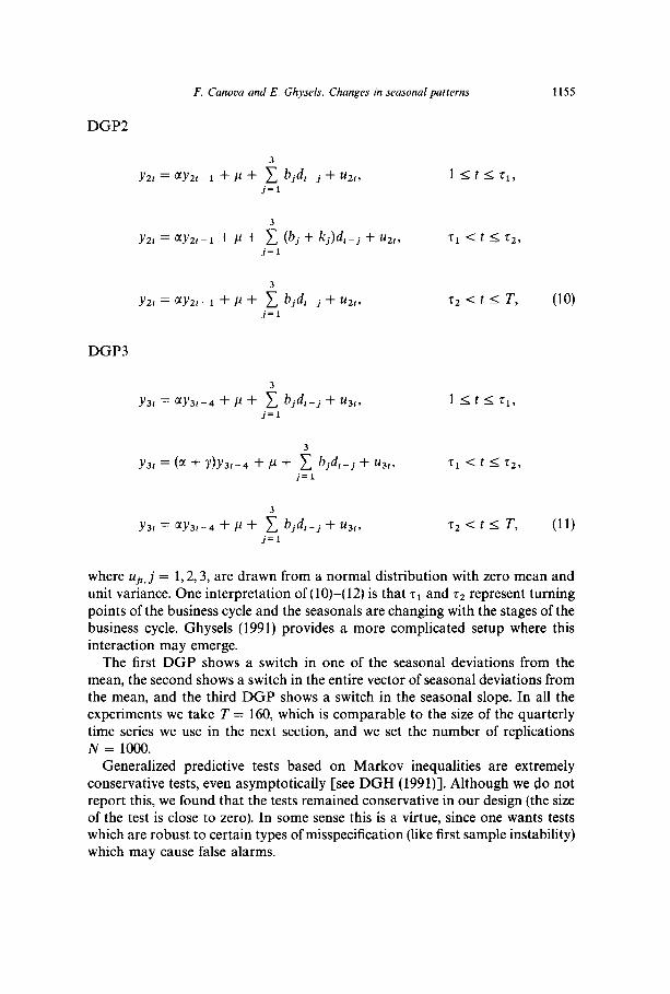
F. Canova and E. Ghysels. Changes in seasonal patterns 1155

DGP2

Yz~ = MYzI-I + P + i b&j + UZ~, j=l

Yz~ = MY,,- I + P + 5 (bj + kj)dt-j + UZ~, j=l

~22 = UY.Z~-I + P + i bjdt-j + ~219 j=l

DGP3

~32 = ~~3t-4 + P + i bj4-j + ~3t3 j=l

3

~32 = (N + Y)YS~-4 + P + 1 bjdt-j + ~3r, j=l

~3t = a~3t-4 + P + i bjdt-j + ~319 j=l

1 stsr1,

71 < t I T2,

z2 < t I T, (10)

lstlz1,

71 -c t I T2,

z2 < t I T, (11)

where Ujt, j = 1,2,3, are drawn from a normal distribution with zero mean and unit variance. One interpretation of (lo)-(12) is that r1 and 52 represent turning points of the business cycle and the seasonals are changing with the stages of the business cycle. Ghysels (1991) provides a more complicated setup where this interaction may emerge.

The first DGP shows a switch in one of the seasonal deviations from the mean, the second shows a switch in the entire vector of seasonal deviations from the mean, and the third DGP shows a switch in the seasonal slope. In all the experiments we take T = 160, which is comparable to the size of the quarterly time series we use in the next section, and we set the number of replications N = 1000.

Generalized predictive tests based on Markov inequalities are extremely conservative tests, even asymptotically [see DGH (1991)]. Although we do not report this, we found that the tests remained conservative in our design (the size of the test is close to zero). In some sense this is a virtue, since one wants tests which are robust to certain types of misspecification (like first sample instability) which may cause false alarms.


We studied the power properties of the test to the timing of the switches in two situations: one where a switch occurs in the estimation sample and the predictive sample T2 starts at the time of the second switch (i.e., T2 = T - z2) and one where a switch occurs in the estimation sample and the predictive sample starts before the time of the break (T2 > T - z2). The two situations we study are ~~ = 40, ~~ = 120, T2 = 40 and r1 = 40, r2 = 130, T2 = 40.

We also studied the power of the test to the magnitude of the switch and to the overall amplitude of seasonal fluctuations. In particular we consider p = [O.O, 6.01, two sets of seasonal coefficients [b,, b2, b3] = [16.0,2.0, 10.01 or [b,, b2, b3] = CO.2 - 0.3,0.3], two values of the seasonal slope a = [O.S,O.l], and two types of switches. For the first DGP and the first set of seasonal coefficients we consider h1 = [l.O, 5.01 and for the second set of seasonal coefficients h1 = [0.2,1.0]. For the second DGP and the first set of coefficients we set [k,, k2, k3] = [l.O, 1.0, 1.01 or [S.O, 5.0,5.0] and for the second set of seasonal coefficients [k,, k2, k3] = [0.2,0.2,0.2] or [l.O, 1.0, 1.01. For the third DGP and both values of a, y = [O.l, 0.43.

Table 1 reports the results for a = 0.5, ~1 = 6.0, and [b,, b2, b3] = [16.0,2.0,10.0]. Table 2 reports the results for a = 0.1, p = 0.0, and [b,, b2, b3] = [0.2, - 0.3,0.3]. In all cases we estimate a model of the type

Yl= i Pjdj+ 5 P~Y~-~ + et (12) j=l q=l

over T1 and construct predictive residuals over T2. In constructing the upper bound to the Markov inequalities we employ the Newey-West procedure with a set of Bartlett weights and a lag window of length 5. In all the experiments we report Q = 4, and in calculating Markov inequalities we set I = 2.

The results indicate that, when the DGP is a switching process, the individual predictive tests are, in general, accurate in detecting the timing of the switch when the magnitude of seasonal fluctuations is large and when the size of switch is large for all three DGP’s. The power of individual predictive tests is also essentially independent of the timing when the predictive sample starts. When the size of the switch is small the tests are very conservative and do not reject the null of no structural breaks when a switch does exist, regardless of the exact timing when the predictive sample starts. This is true both when the magnitude of seasonal fluctuations is large and also when seasonal fluctuations are minor.

The power of joint yearly test is slightly different across DGP’s. When only one intercept is switching, the test is not very powerful in detecting the timing of the switch regardless of the magnitude of the change, but when the switch occurs in the entire vector of intercepts or in the slope, the test identifies the timing of the break with sufficient precision. Once again the exact timing of the shift is not crucial, as long as it occurs in the predictive sample.

Tab

le

1

Pow

er

of G

PT

test

s,

case

of

sw

itchi

ng

proc

ess.

”

Sam

ple

size

T

=

160,

est

imat

ion

sam

ple

Ti

= 12

0, p

redi

ctiv

e sa

mpl

e r,

= 40

, re

plic

atio

ns

N

= 10

00,

fi =

0.

5,

n =

6.0,

b =

11

6.0,

2.

0,

10.0

1.

Lar

ge

jum

p Sm

all

jum

p

Tes

t

r, =

40,

r* =

12

0 r1

=

40,

r* =

13

0 5,

=

40,

r2 =

12

0 5,

=

40,

72 =

13

0

DG

Pl

DG

P2

DG

P3

DG

Pl

DG

P2

DG

P3

DG

Pl

DG

P2

DG

P3

DG

Pl

DG

P2

DG

P3

IPT

M

ax.

53.4

89

.2

100.

0 53

.2

85.9

99

.4

1.2

1.6

17.4

1.

2 1.

2 12

.8

Loc

atio

n 12

1 12

1 12

1 13

3 13

1 13

1 12

9 12

4 12

1 13

0 13

1 13

3

YP

T

1 14

.0

33.4

2

0.0

0.0

3 0.

0 0.

0 4

0.0

0.0

5 0.

0 0.

0 6

0.0

0.0

7 0.

0 0.

0 8

0.0

0.0

9 0.

0 0.

0 10

0.

0 0.

0

100.

0 97

.6

0.6

I 0.

0 0.

0 0.

0 0.

0 0.

0 0.

0

0.0

0.0

0.0

2.6

6.2

10.1

0.

0 0.

0 0.

0 0.

0 0.

0 0.

0 0.

0 0.

0 0.

0 0.

0 0.

0 0.

0 0.

0 0.

0 0.

0 0.

0 0.

0 0.

0 0.

0 0.

0 0.

0 10

.5

20.4

10

0.0

0.0

0.0

0.0

0.2

2.0

8.6

0.6

0.0

100.

0 0.

0 0.

0 0.

0 0.

0 0.

0 0.

2 0.

0 0.

0 10

0.0

0.0

0.0

0.0

0.0

0.0

0.0

0.0

0.0

89.4

0.

0 0.

0 0.

0 0.

0 0.

0 0.

0 0.

0 0.

0 0.

0 0.

0 0.

0 0.

0 0.

0 0.

0 0.

0 0.

0 0.

0 0.

0 0.

0 0.

0 0.

0 0.

0 0.

0 0.

0 0.

0 0.

0 0.

0 0.

0 0.

0 0.

0 0.

0 0.

0 0.

0

SPT

1

0.0

0.0

100.

0 0.

0 0.

0 10

0.0

0.0

0.0

3.1

0.0

0.0

2.7

2 0.

0 0.

0 0.

0 0.

0 0.

0 0.

0 0.

0 0.

0 0.

0 0.

0 0.

0 0.

0 3

0.0

0.0

0.0

0.0

0.0

0.0

0.0

0.0

0.0

0.0

0.0

0.0

4 0.

0 0.

0 0.

0 0.

0 0.

0 0.

0 0.

0 0.

0 0.

0 0.

0 0.

0 0.

0

OPT

1

0.0

0.0

99.4

0.

0 0.

0 10

0.0

0.0

0.0

0.0

0.0

0.0

0.0

“For

al

l th

ree

DG

P’s

the

proc

ess

jum

ps

at t

i +

1 an

d ge

ts

back

to

the

ori

gina

l va

lues

at

TV

+

1. A

lar

ge

jum

p fo

r D

GPl

is

h,,

= [S

.O,O

.O, 0

.01;

for

DG

PZ,

k,,

= [5

.0,5

.0,

5.01

; fo

r D

GP3

, yi

=

0.4.

A

sm

all

jum

p fo

r D

GPl

is

hi,

= [l

.O,O

.O,O

.O];

fo

r D

GP2

, k,

, =

[l.O

, 1.

0, 1

.01;

for

D

GP3

, yi

=

0.1.

IP

T

is t

he

indi

vidu

al

peri

od

pred

ictiv

e te

st,

YT

P

is t

he

year

ly

pred

ictiv

e te

st

(ass

umin

g ob

serv

atio

ns

are

quar

ters

),

SPT

is

the

se

ason

pr

edic

tive

test

, an

d O

PT

is t

he

over

all

pred

ictiv

e te

st.

The

ta

ble

repo

rts

the

perc

enta

ge

of r

eplic

atio

ns

for

whi

ch

the

test

re

ject

s th

e nu

ll hy

poth

esis

of

no

chan

ges

at

the

10%

si

gnif

ican

ce

leve

l. Fo

r IP

T

we

only

re

port

th

e m

axim

um

perc

enta

ge

of r

eplic

atio

ns

for

whi

ch

the

test

re

ject

s th

e nu

ll hy

poth

esis

an

d th

e lo

catio

n w

here

th

e m

axim

um

occu

rs.

Tab

le

2

Pow

er

of G

PT

test

s,

case

of

sw

itchi

ng

proc

ess.

”

Sam

ple

size

T

=

160,

est

imat

ion

sam

ple

T,

= 12

0, p

redi

ctiv

e sa

mpl

e r,

= 40

, re

plic

atio

ns

N =

10

00,

/j =

0.1,

p =

0.0

, h

= [0

.2,

- 0.

3,

0.31

.

Lar

ge

jum

p Sm

all

jum

p

rr

= 40

, r*

=

120

tr

= 40

, r2

=

130

rr

= 40

, rZ

=

120

rr

= 40

, T

Z =

13

0

DG

Pl

DG

P2

DG

P3

DG

Pl

DG

P2

DG

P3

DG

Pl

DG

P2

DG

P3

DG

Pl

DG

P2

DG

P3

IPT

M

ax.

11.2

19

.8

30.8

10

.9

17.2

23

.4

0.6

0.5

2.4

1.2

1.0

2.1

Loc

atio

n 12

8 12

7 12

3 14

3 15

0 13

8 13

5 12

6 12

5 14

0 13

9 13

7

YP

T

1 1.

1 2.

5 3.

7 0.

0 0.

0 0.

0 0.

6 0.

8 1.

1 0.

0 0.

0 0.

0 2

0.0

0.0

0.0

0.0

0.0

0.0

0.0

0.0

0.0

0.0

0.0

0.0

3 0.

0 0.

0 0.

0 0.

0 0.

0 0.

0 0.

0 0.

0 0.

0 0.

0 0.

0 0.

0 4

0.0

0.0

0.0

0.6

2.1

3.0

0.0

0.0

0.0

0.2

1.0

1.8

5 0.

0 0.

0 0.

0 0.

6 0.

0 0.

0 0.

0 0.

0 0.

0 0.

0 0.

0 0.

0 6

0.0

0.0

0.0

0.0

0.0

0.0

0.0

0.0

0.0

0.0

0.0

0.0

7 0.

0 0.

0 0.

0 0.

0 0.

0 0.

0 0.

0 0.

0 0.

0 0.

0 0.

0 0.

0 8

0.0

0.0

0.0

0.0

0.0

0.0

0.0

0.0

0.0

0.0

0.0

0.0

9 0.

0 0.

0 0.

0 0.

0 0.

0 0.

0 0.

0 0.

0 0.

0 0.

0 0.

0 0.

0 10

0.

0 0.

0 0.

0 0.

0 0.

0 0.

0 0.

0 0.

0 0.

0 0.

0 0.

0 0.

0

SPT

1

0.0

0.0

2.1

0.0

0.0

2.3

0.0

0.0

0.7

0.0

0.0

0.9

2 0.

0 0.

0 0.

0 0.

0 0.

0 0.

0 0.

0 0.

0 0.

0 0.

0 0.

0 0.

0 3

0.0

0.0

0.0

0.0

0.0

0.0

0.0

0.0

0.0

0.0

0.0

0.0

4 0.

0 0.

0 0.

0 0.

0 0.

0 0.

0 0.

0 0.

0 0.

0 0.

0 0.

0 0.

0

OPT

1

0.0

0.0

0.0

0.0

0.0

0.0

0.0

0.0

0.0

0.0

0.0

0.0

“For

al

l th

ree

DG

P’s

the

proc

ess

jum

ps

at r

, +

1 an

d ge

ts

back

to

the

ori

gina

l va

lues

at

r2

+ 1.

A l

arge

jum

p fo

r D

GPl

is

h,,

= [l

.O,

O.O

,O.O

]; fo

r D

GPZ

, k,

, =

[l.O

, 1.

0, 1

.01;

for

D

GP3

, y,

=

0.4.

A

sm

all

jum

p fo

r D

GPl

is

hr,

= [0

.2,0

.0,0

.0];

fo

r D

GP2

, k,

, =

[0.2

,0.2

,0.2

];

for

DG

P3,

y,

= 0.

1.

IPT

is

the

in

divi

dual

pe

riod

pr

edic

tive

test

, Y

TP

is

the

ye

arly

pr

edic

tive

test

(a

ssum

ing

obse

rvat

ions

ar

e qu

arte

rs),

SP

T

is t

he

seas

on

pred

ictiv

e te

st,

and

OPT

is

the

ov

eral

l pr

edic

tive

test

. T

he

tabl

e re

port

s th

e pe

rcen

tage

of

rep

licat

ions

fo

r w

hich

th

e te

st

reje

cts

the

null

hypo

thes

is

of n

o ch

ange

s at

the

10

%

sign

ific

ance

le

vel.

For

IPT

w

e on

ly

repo

rt

the

max

imum

pe

rcen

tage

of

rep

licat

ions

fo

r w

hich

th

e te

st

reje

cts

the

null

hypo

thes

is

and

the

loca

tion

whe

re

the

max

imum

oc

curs

.


The joint season and overall tests detect the presence of structural breaks only in the case where the switch is large enough and where it persistently changes the pattern of that season. For example, a switch in one seasonal intercept is not

sufficient for the joint seasonal and overall tests to reject the null. However, when we consider large enough switches in the seasonal slope, the tests always reject the null. Also in this case the intensity of the seasonal fluctuations, more than the size of the switch, is important in determining the power of the test for all three DGP’s.

Although we report results only for a limited set of experiments, it is worth mentioning that we also conducted several additional exercises such as changing the number of lags in the estimated model (i.e., changing Q from 2 to 6), adding switches in the estimation sample or in the predictive sample. Depending on the exact specification, the results are slightly altered, but the basic message of the exercise is maintained. The tests are in general powerful in detecting a break and in correctly selecting its timing when seasonal fluctuations are significant and the size of the switch is large, regardless of the exact selection of other parameters. The power however deteriorates when the size of the switch or the magnitude of the seasonal fluctuations is negligible.

In sum, when the DGP is a switching type process the tests are more conservative than in the case when the DGP is stable in the estimation sample and structural breaks occur only in the predictive sample, but the power is independent of the exact starting period of the predictive sample. There are two implications of these results. First, if we find evidence of instability in the estimation sample and if the tests detect changes in the seasonal patterns in the predictive sample, we can be confident that the underlying time series has really changed in a dramatic manner and that the tests have not given a false alarm. Evidence of instability of first sample estimates will be examined in detail for each data set. Second, the exact selection of T1 and T2 is somewhat irrelevant so long as there is a break in T2. This allows an arbitrary division of the sample period in estimation and predictive samples and reduces the scope for data mining connected with the choice of the ending date of the estimation period. In the next section, we will choose the estimation sample to be equal to 75% of the entire data set, while the prediction sample represents the remaining 25%.

4. An empirical investigation

4.1. The data

We apply generalized predictive tests to two data sets. Details on the sources of the data are provided in the appendix of Canova and Ghysels (1992). The first data set was originally examined by Barsky and Miron (1989) in their study of the seasonal and cyclical fluctuations and includes all the major aggregate seasonally nonadjusted US macroeconomic series. For all series but


the monetary base, the money multiplier, hours, and wage, T1 ends in 1974.1. For the monetary base and the money multiplier, T1 ends in 1977.1. For hours and wage, T1 ends in 1980.1. The upper bound of the Markov inequalities are constructed using a Newey-West procedure with a Bartlett window of length m = 5 for all series but hours and wage, for which we set m = 4, as suggested by Andrews (1991). The lag length p in (1) is equal to 5 for all series.

The second data set is the same used by Beaulieu and Miron (1991). For reason of space we concentrate on the attributes of three industries, two from the nondurable category (textile and petroleum) and one from the durable category (machinery), which appear to be sensitive to business cycle conditions. For all series p = 13, m = 4, and T1 ends in 1980.1 except for HOURS and EMPL where T1 ends in 1977.1.

For all series we present results obtained using a log first-difference transformation of the data and set r = 2. In order to study the sensitivity of the results to different stationary inducing transformation we also considered two other procedures: a polynomial detrending and a seasonal first-order differencing. We also studied the sensitivity of the results to changes in r setting Y = 1. Although numerical values of the Markov inequalities change, the basic message of the exercises is unchanged by these experiments. One reason for the robustness of our conclusions is that to apply GPT we only need consistency of parameter estimates and martingale differenced residuals and as long as the lag length of the autoregression p in (1) is approximately correct, consistency is ensured regardless of the detrending transformation used.

Before discussing the results we examine whether model (1) is unstable over T, with each data set. Besides helping to decide whether the resulting p-values are conservative or not, this exercise is also useful because it may give some economic information on the evolution of seasonals over time. For this purpose we compute recursive residuals for each series in each data set in the first sample and perform sequential Chow tests for the stability of the estimates. The results suggest that for the first data set T, is essentially stable except perhaps for the unemployment, the labor force, and the wage series. It is also worth mentioning that, although not statistically significant, many aggregate series display increased heteroskedasticity around the turning points of the business cycles. The second data set is more supportive of the assumption of a stable first sample. For many series we found almost no evidence of structural instability. The exceptions are production and shipments in the textile industry, whose residuals display increased volatility after 1978, and hours and employment in the petroleum industry, which show outliers in 1953 and 1969, respectively.

4.2. Post- WWII US aggregately quarterly macro variables

For many variables in this data set there is a tendency for the p-values of the Markov inequalities for IPT to go below the 5% mark during the three


recessions of the prediction sample. This tendency however is not generalized. For example, the three labor series (unemployment, employment, and labor force) and the money multiplier series do not display statistically significant evidence of instabilities, even though the unemployment rate displays important spikes in the p-values during recessions (see fig. 3), while series like consumption

Fig. 3. Aggregated quarterly macro series, p-values for Markov inequalities.

F. Canova and E. Ghysels. Changes in seasonal patterns

Fig. 3 (continued)

of services, imports, and Ml pass the 5% mark both in expansions and in recessions. In addition, the effects of recessions are not all alike over time. While during the 1974-75 recession structural changes appear to be minor (the basic exceptions here are the three consumption series), a clear pattern of instabilities

Tab

le

3

Agg

rega

te

quar

terl

y po

st-W

WII

da

ta.”

P-va

lues

fo

r jo

int

Mar

kov

ineq

ualit

ies,

sa

mpl

e 19

74.1

L19

85.4

.

Var

iabl

e 19

74

1975

19

76

1977

19

78

1979

19

80

1981

19

82

1983

19

84

1985

Sp

ring

Su

mm

er

Fall

Win

ter

Ove

rall

IFIX

IFIXR

IFIXNR

IFIXNRS

IFIXNRPD

CNS

CND

CDUR

CSER

GNP

GOVFED

IMPORT

EXPORT

BUSINV

FINSALE

CPI

T-BILL

MI

UNEMP

LABFOR

EMPL

MONBASE

MONMULT

WAGE

HOURS

0.30

0.

56

0.12

0.

07

0.05

0.

27

0.33

0.

11

0.03

0.

06

1.00

0.

49

0.28

0.

07

0.09

0.

27

0.18

0.

38

0.17

0.

06

1.00

0.

68

0.21

0.

04

0.17

0.

11

0.23

0.

33

0.16

0.

12

0.27

0.

29

0.28

0.

10

0.10

0.

08

0.13

0.

63

0.14

0.

06

0.17

0.

17

0.05

0.

05

0.05

0.

08

0.15

1.

00

0.08

0.

06

1.00

1.

00

0.8

1 0.

94

0.19

0.

06

0.02

0.

05

0.76

0.

22

0.11

0.

09

0.37

0.

19

0.03

0.

31

0.07

0.

46

0.29

1.

00

0.12

0.

30

0.35

0.

07

0.04

0.

28

0.54

1.

00

0.38

0.

13

0.28

0.

39

1.00

1.

00

0.23

1.

00

0.07

0.

11

0.26

0.

06

1.00

0.

32

1.00

1.

00

1.00

0.

63

1.00

0.

69

1.00

1.

00

0.35

0.

19

0.41

0.

54

0.60

0.

59

0.18

1.

00

0.22

0.49

0.

16

0.27

0.

07

0.08

0.

07

0.09

0.

11

0.03

0.

21

0.12

0.

04

0.18

0.

13

0.09

0.08

0.04

0.09

0.02

0.04

0.11

0.

09

0.01

0.

02

0.18

0.

04

0.08

0.

01

0.02

0.

68

1.00

0.

66

0.10

0.14

0.25

0.40

0.02

0.

02

0.05

0.

01

0.11

0.

09

0.06

0.

08

0.02

0.

06

0.04

0.

02

0.06

0.

03

0.08

0.

10

0.03

1.00

1.

00

0.67

0.

06

0.31

0.

34

1.00

0.01

0.

02

0.02

0.

03

0.02

0.

01

0.10

0.

07

0.03

0.

01

1.00

0.

82

0.04

0.

24

0.41

0.

27

1.00

0.01

0.

01

0.01

0.

01

0.01

0.

02

0.06

0.

02

0.01

0.

04

0.04

0.

00

0.02

0.

04

0.01

0.

11

0.84

0.

03

1.00

0.

40

0.08

0.

12

0.31

0.

34

0.48

0.01

0.

03

0.06

0.

01

0.02

0.

05

0.01

0.

01

0.02

0.

03

0.12

0.

01

0.02

0.

23

0.05

0.

02

0.05

0.

04

0.12

0.

01

0.10

0.

04

0.03

0.

05

0.03

0.

03

0.03

0.

06

0.05

0.

01

0.04

0.

02

0.00

0.

00

0.00

0.

02

0.03

0.

01

0.01

0.

03

0.04

0.

01

0.13

0.

03

0.03

0.

00

0.00

0.

01

0.15

0.

02

0.08

0.

05

0.00

0.

03

0.02

0.

07

0.07

0.

03

0.03

0.

02

0.62

0.

35

0.16

0.

05

0.57

0.

58

0.14

0.

12

0.07

0.

02

0.02

0.

01

1.00

1.

00

1.00

1.

00

0.60

1.

00

1.00

0.

89

0.13

0.

99

0.08

0.

15

0.24

0.

08

0.14

0.

15

0.63

0.

49

0.71

0.

25

0.43

0.

82

1.00

0.

56

1.00

1.

00

1.00

1.

00

0.03

0.

02

0.06

0.

04

0.07

0.

07

0.06

0.

01

0.02

0.

04

0.16

0.

00

0.01

0.

05

0.02

0.

10

0.03

0.

03

0.97

0.62

0.45

0.12

0.25

0.30

1.00

0.06

0.

05

0.03

0.

02

0.04

0.86

0.45

0.19

0.23

0.50

0.66

1.00

0.02

0.

02

0.04

0.

03

0.04

0.

04

0.05

0.

03

0.00

0.

03

0.04

0.

00

0.02

0.

02

0.04

0.

10

0.06

0.

02

1.00

0.

78

0.15

0.

15

0.32

0.

74

1.00

“The

ye

ar

entr

y re

fers

to

the

te

st

for

the

join

t be

havi

or

of t

hat

year

. T

he

seas

on

entr

y re

fers

to

the

joi

nt

beha

vior

of

tha

t se

ason

ov

er

all

the

year

s of

the

sa

mpl

e.

Ove

rall

refe

rs

to

a te

st

for

all

the

year

s in

th

e sa

mpl

e.


emerge in the last two recessions (1979-81) and (1981-82), with a strong concentration of structural changes during the 1981-82 contraction.

The joint annual tests (see table 3) strengthen the results of the ITP and confirm (i) the emergence of structural instabilities primarily in the last two recessions of the sample and (ii) a tendency of seasonals toward long-run drifts. The joint season tests provide further evidence that the seasonals of most series in this data set are unstable. The exceptions here are the labor force, the unemployment rate, and the wage series. All these series displayed some instability in the first sample, so that while there is no statistical tendency for structural changes one should keep in mind that the p-values are conservative. Overall, the season which appears to be the most unstable is summer, but the differences across seasons are minor.

4.3. Post- WWII disaggregated monthly macro variables

The evidence emerging from the second data set is supportive of the idea that business cycle fluctuation play a nontrivial effect on the pattern of seasonality of existing disaggregated time series (see table 4). For reason of space we only report JPT for this data set. Graphs of IPT are contained in Canova and Ghysels (1992). If we exclude the price level in the petroleum industry and shipments in the machinery industry, there is a tendency for the p-value of the Markov inequalities of IPT for many series to pass the 5% bound exactly in recessions. It is also worth emphasizing that because of the relatively small sample size available for production, shipment, and prices (20 years), the 5% mark for the Markov inequality is probably too demanding and one should look for tendencies more than for direct violation of this bound.

Although not completely significant from the statistical point of view, the evidence provided by the employment series in all three industries is economically important. The only time when seasonals appear to be moving is during recessions. One can think of many explanations for this pattern. Given the existing rigidities in adjusting employment levels, the most obvious one seems that, in recessions, firms provide longer vacation time for workers, therefore altering the existing pattern of seasonality in employment.

The joint tests also support these results. All series but employment in the petroleum industry display both changes in their joint yearly pattern as well as changes in the pattern of months in the sample. The exception here is the employment series in the petroleum industry, which displays instabilities when individual months are considered, but, over the year, these instabilities appear to average out.

5. The costs of treating seasonality as constant

The last section has provided evidence suggesting that the seasonal patterns of many macro variables are unstable and that the instabilities are perhaps

Tab

le

4

Dis

aggr

egat

ed

mon

thly

po

st-W

WII

da

ta.”

P-va

lues

fo

r jo

int

Mar

kov

ineq

ualit

ies,

sa

mpl

e 19

77.1

-198

7.12

.

Y42

2 Y

429

Y43

5 SP

22

SP29

SP

35

PR22

PR

29

PR35

E

MP2

2 E

MP2

9 E

MP3

5 P

DH

R22

P

DH

R29

P

DH

R35

1977

1.

00

1.00

0.

02

0.02

0.

41

0.02

19

78

1.00

1.

00

0.14

0.

09

0.22

0.

03

1979

1.

00

1.00

0.

08

0.06

0.

12

0.03

19

80

1.00

1.

00

0.01

0.

02

0.00

0.

01

1981

0.

23

0.02

0.

02

0.05

0.

03

0.06

19

82

0.01

0.

01

0.01

0.

02

0.00

0.

02

0.03

0.

05

0.04

0.

43

1.00

0.

04

0.00

0.

16

0.01

19

83

0.01

0.

00

0.01

0.

02

0.00

0.

03

0.02

0.

01

0.08

0.

16

1.00

0.

02

0.00

0.

09

0.03

19

84

0.00

0.

00

0.01

0.

01

0.00

0.

01

0.05

0.

04

0.06

1.

00

1.00

0.

05

0.02

0.

17

0.06

19

85

0.00

0.

00

0.00

0.

02

0.00

0.

00

0.02

0.

04

0.16

0.

61

1.00

0.

15

0.04

0.

24

0.08

19

86

0.00

0.

00

0.00

0.

03

0.02

0.

00

0.06

0.

01

0.08

0.

49

1.00

0.

27

0.02

0.

06

0.04

19

87

0.00

0.

00

0.00

0.

02

0.00

0.

00

0.10

0.

00

0.10

0.

94

1.00

0.

37

0.03

0.

17

0.10

Janu

ary

0.00

0.

00

0.00

0.

01

0.00

0.

01

0.00

0.

00

0.01

0.

03

0.00

0.

00

0.01

0.

01

0.00

Fe

brua

ry

0.00

0.

01

0.00

0.

02

OIK

I 0.

00

0.03

0.

05

0.01

1.

00

0.02

0.

01

0.00

0.

00

0.00

M

arch

0.

32

0.00

0.

00

1.00

0.

00

0.00

0.

00

0.00

0.

01

0.05

0.

03

0.00

0.

00

0.01

0.

01

Apr

il 0.

00

0.00

0.

00

0.04

0.

01

0.00

0.

09

0.00

0.

14

0.03

0.

20

0.00

0.

01

1.00

0.

02

May

0.

00

0.00

0.

00

0.00

0.

00

0.00

0.

01

0.00

0.

02

0.00

0.

01

0.00

0.

05

0.02

0.

00

June

0.

00

0.04

0.

00

0.02

0.

06

0.00

0.

09

0.00

0.

00

0.12

0.

00

0.01

0.

00

0.01

0.

01

July

0.

19

0.01

0.

00

0.00

0.

01

0.00

0.

00

0.00

0.

03

0.28

0.

08

0.03

0.

02

0.00

0.

01

Aug

ust

0.00

0.

01

0.00

0.

04

0.00

0.

00

0.02

0.

00

0.02

0.

11

0.00

0.

00

0.01

0.

02

0.01

Se

ptem

ber

0.02

0.

02

0.00

0.

04

0.00

0.

00

0.74

0.

00

0.00

0.

05

0.02

0.

06

0.09

0.

00

0.00

O

ctob

er

0.00

0.

01

0.26

0.

00

0.00

0.

03

0.00

0.

00

0.06

0.

05

0.01

0.

05

0.01

0.

00

0.00

N

ovem

ber

0.00

0.

00

0.01

0.

02

0.00

0.

00

0.00

0.

00

0.01

0.

03

0.00

0.

01

0.04

0.

00

0.01

D

ecem

ber

0.00

0.

01

0.00

O

.tXl

0.00

0.

00

0.02

0.

00

0.97

0.

06

1.00

0.

00

0.00

0.

00

0.00

Ove

rall

0.00

0.

00

0.00

0.

00

0.00

0.

00

0.00

0.

00

0.00

0.

00

0.00

0.

00

0.00

0.

00

0.00

“The

ye

ar

entr

y re

fers

to

the

te

st

for

the

join

t be

havi

or

of t

hat

year

. T

he

mon

th

entr

y re

fers

to

the

joi

nt

beha

vior

of

tha

t m

onth

ov

er

all

the

year

s of

the

se

cond

sa

mpl

e.

Ove

rall

refe

rs

to a

tes

ts

for

the

join

t be

havi

or

over

th

e en

tire

sam

ple.

Y

4 ar

e ou

tput

se

ries

, SH

are

sh

ipm

ent

seri

es,

PR

are

pr

ice

seri

es,

EM

P

empl

oym

ent

seri

es,

and

PD

HR

ar

e pr

oduc

tion

hour

s,

Indu

stry

22

is

text

ile,

indu

stry

29

is

petr

oleu

m,

and

indu

stry

35

is

mac

hine

ry.


related to business cycle fluctuations. To determine the costs a researcher incurs by assuming a model in which seasonals are represented by time-invariant deterministic dummies, when the actual DGP for the seasonals varies with the stages of the business cycle, we conduct a simple forecasting exercise. Ghysels, Lee, and Siklos (1992) examine the effects of incorrectly specifying the seasonal component of a series from the point of view of the univariate time series properties of the data.

To determine the forecasting costs of a wrong model specification we construct a statistic similar to the Theil-U. The denominator of the statistic is the Mean Square Error (MSE) of a model whose seasonals are treated as constant over time (seasonal dummy model). The numerator is either the MSE of a model where seasonal dummies are allowed to change with the stages of the business cycle [as in Ghysels (1990)] or the MSE of a model where the coefficients of the dummies are allowed to drift over time according to a Litterman-type prior [as in Canova (1992)]. This statistic provides a useful measure of the forecasting performance of alternative models, allows a rough calculation of the gains obtained by taking into account the evidence we uncovered in previous sections, and has a very simple interpretation. If a value less than 1 obtains, the model with changing seasonals dominates in MSE terms a model with constant deterministic dummies, and vice versa if a value greater than 1 obtains. The three model specifications we employ are given by (1) and by

S-l

xt = P + C (4s + Xt6_Jdf + i ajxt-j + clzt + vlt s=l j=l

and

S-l

xt = P + 1 &.vtdf + f ajtX,-j + c(Z, + f/f, s=l i= 1

(13)

(14)

where xt is a dummy variable which is equal to 1 if the economy is in an expansion according to NBER chronology and 0 otherwise, d,‘s are seasonal dummies, z, is a linear time trend, fii = [41t, . . . , 4st, al,, . . . , ajt, p, ~11, G = block- diag[Gl,Gz] with Gl = fJZl*Z and G2 = I, u; = [ulr,O], E,[u,,,u~,] = a:, = diag[a:] * e2, where 8i and tZ2 are hyperparameters which will be selected with a rough specification search as described by Litterman (1986). In all three specifications, p lags of x, are included to prewhiten the residuals.

In the exercises we focus attention on changes in the coefficient representing seasonal deviations from the overall mean so that in (14) and (15)-(16) only the coefficients of the dummies are allowed to vary over time. All other coefficients


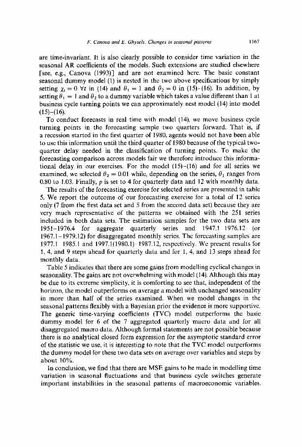
are time-invariant. It is also clearly possible to consider time variation in the seasonal AR coefficients of the models. Such extensions are studied elsewhere [see, e.g., Canova (1993)] and are not examined here. The basic constant seasonal dummy model (1) is nested in the two above specifications by simply setting xt = 0 Vt in (14) and e1 = 1 and e2 = 0 in (15)-(16). In addition, by setting 8i = 1 and d2 to a dummy variable which takes a value different than 1 at business cycle turning points we can approximately nest model (14) into model

(15)-(16). To conduct forecasts in real time with model (14), we move business cycle

turning points in the forecasting sample two quarters forward. That is, if a recession started in the first quarter of 1980, agents would not have been able to use this information until the third quarter of 1980 because of the typical two- quarter delay needed in the classification of turning points. To make the forecasting comparison across models fair we therefore introduce this informa- tional delay in our exercises. For the model (15)-(16) and for all series we examined, we selected G2 = 0.01 while, depending on the series, 8r ranges from 0.80 to 1.03. Finally, p is set to 4 for quarterly data and 12 with monthly data.

The results of the forecasting exercise for selected series are presented in table 5. We report the outcome of our forecasting exercise for a total of 12 series only (7 from the first data set and 5 from the second data set) because they are very much representative of the patterns we obtained with the 251 series included in both data sets. The estimation samples for the two data sets are 1951-1976.4 for aggregate quarterly series and 1947.1-1976.12 (or 1967.1- 1979.12) for disaggregated monthly series. The forecasting samples are 1977.1-1985.1 and 1997.1(1980.1)-1987.12, respectively. We present results for 1, 4, and 9 steps ahead for quarterly data and for 1,4, and 13 steps ahead for monthly data.

Table 5 indicates that there are some gains from modelling cyclical changes in seasonality. The gains are not overwhelming with model (14). Although this may be due to its extreme simplicity, it is comforting to see that, independent of the horizon, the model outperforms on average a model with unchanged seasonality in more than half of the series examined. When we model changes in the seasonal patterns flexibly with a Bayesian prior the evidence is more supportive. The generic time-varying coefficients (TVC) model outperforms the basic dummy model for 6 of the 7 aggregated quarterly macro data and for all disaggregated macro data. Although formal statements are not possible because there is no analytical closed form expression for the asymptotic standard error of the statistic we use, it is interesting to note that the TVC model outperforms the dummy model for these two data sets on average over variables and steps by about 10%.

In conclusion, we find that there are MSE gains to be made in modelling time variation in seasonal fluctuations and that business cycle switches generate important instabilities in the seasonal patterns of macroeconomic variables.


Variable

Table 5

Forecasting comparison, modified U-statistic.B

Interactive model Time-varying model

1 4 9 13 1 4 9 13

Aggregate quarterly macro data, forecasting sample 1977.1-1985.4

GNP 1.00 1.00 1.03 0.95 0.95 0.92 IFIX 1.00 1.01 1.02 0.94 0.97 0.98 CDUR 1.00 1.00 1.00 0.98 0.99 0.93 Ml 1.00 1.00 0.99 0.98 1.00 1.00 EMPL 0.93 0.94 1.04 0.97 0.92 1.00 FINSALE 0.99 0.99 1.01 0.95 0.97 0.86 MONMULT 0.98 0.96 0.94 0.96 1.02 0.98

Disaggregate monthly macro data, forecasting sample 1977.1(1980.1)-1987.12

Y435 0.97 0.97 0.98 0.78 0.79 0.87 SH35 0.99 0.99 1.00 0.68 0.67 0.80 PR35 1.08 1.11 1.08 0.67 0.66 0.74

EMP35 0.90 0.90 0.89 0.99 0.99 0.98 HO URS35 1.00 1.00 1.01 0.99 1.02 1.00

“In the aggregate macro data GNP is gross national product, IFIX is fixed investments, CDUR is consumption of durables, Ml is money, EMPL is employment, FINSALE is final sales, MON- MULT is the money multiplier. The disaggregate macro data refer to industry 35 (machinery), and Y4 is a measure of output, SH is a measure of shipments, PR is the price of output, EMP is a measure of employment, and HOURS is a measure of production hours. ‘Interactive model’ refers to a model where seasonal deviations from the mean are interacted with a cyclical dummy. ‘Time-varying model’ refers to a model where time variations in the seasonal deviations from the mean are flexibly modelled with a Bayesian prior.

Although more evidence must be collected before general conclusions can be drawn, the results we present indicate that the forecasting costs of taking a short-cut approach to account for seasonal fluctuations may be substantial.

6. Conclusions

This paper documents the existence of instabilities in seasonal patterns for a large class of US time series, including quarterly and monthly aggregated and disaggregated data, and attempts to link these instabilities to the stages of the business cycle. In documenting the pattern of instabilities we rely both on the graphical technique and on recently developed tests for structural stability for dynamic systems as proposed by Dufour, Ghysels, and Hall (1991). This testing methodology is particularly suited to examine the hypothesis of cyclicality of seasonal patterns because it can detect single or multiple shifts that are either temporary or permanent in nature.


We find that for the majority of the aggregated US time series examined seasonals drift over time and, in some cases, these changes are linked to the stages of the business cycle. The evidence for disaggregated data is less statistically significant but more compelling from the economic point of view, since changes appear to occur primarily in recession. We demonstrated with a simple forecasting exercise that there are gains to be made by taking into account the time structure of seasonal instabilities. In particular, by allowing a flexible pattern of time variation in the seasonal dummies we find that one can improve (in MSE terms) the forecasting performance of a model with constant seasonals by 10% on average.

The results of this paper have a number of interesting implications for those who are interested in characterizing the properties of cyclical and seasonal fluctuations in macro aggregates and wish to examine the validity of models using the restrictions implied by the interaction between various components of the series. First, cataloging business cycle facts with seasonally adjusted data is improper unless the seasonal adjustment takes into account the particular form of interaction existing among the components of the series (and this is seldom the case). Second, aggregate macroeconomic models should explicitly examine not only seasonal fluctuations but also the seasonal and cyclical interaction in order to provide guidelines to organize the facts we have described in this paper. Third, the asymmetric behavior of seasonals over the business cycle makes it clear that linear-quadratic models or models which are linear-quadratically approximated around the steady state are incapable of capturing important features of the data. Theoretical models with some form of threshold may be more useful in characterizing the cyclical/seasonal properties of the data. Finally, the observation that the sectoral monthly employment series displays the most interesting economic variations in seasonal patterns while the aggregate quarterly employment series does not, speaks against the use of representative agent general equilibrium models. It also suggests that rigidities in sectoral labor markets may generate these nonlinear effects in macroeconomic time series.

References

Andrews, D., 1991, Heteroskedasticity and autocorrelation consistent covariance matrix estimation, Econometrica 59, 817-859.

Andrews, D. and R. Fair, 1988, Inference in econometric models with structural change, Review of Economic Studies LV, 615-640.

Barskv. R.B. and J.A. Miron. 1989, The seasonal cvcle and the business cycle, Journal of Political Economy 97, 503-534.

Beaulieu, J. and J.A. Miron, 1991, Seasonality in manufacturing, Economics Letters 36, 345-351. Beaulieu, J. and J.A. Miron, 1993, Seasonal unit roots in US aggregate data, Journal of Econo-

metrics 55, 306-328. Bell. W.R. and S.C. Hillmer. 1984. Issues involved with the seasonal adiustment of economic time

series, Journal of Business and Economic Statistics 2, 526-534.


Brown, R., J. Durbin, and M. Evans, 1975, Techniques for testing the constancy of regression relationships over time, Journal of the Royal Statistical Society B 37, 149-163.

Canova, F., 1992, Detrending and business cycle facts, Manuscript (European University Institute, San Domenico di Fiesole).

Canova, F., 1993, Forecasting a multitude of series with common seasonal patterns, Journal of Econometrics 55, 173-202.

Canova, F. and E. Ghysels, 1992, Changes in the seasonal patterns: Are they cyclical?, CRDE discussion paper 1692 (University of Montreal, Montreal).

Canova, F. and B. Hansen, 1991, Are seasonal patterns constant over time? A test for seasonal stability, Manuscript (University of Rochester, Rochester, NY).

Chow, G., 1960, Tests ofequality between sets ofcoefficients in two linear regressions, Econometrica 28, 591-605.

Dickey, D., D. Hasza, and W. Fuller, 1984, Testing for unit roots in seasonal time series models, Journal of the American Statistical Association 79, 355-367.

Dufour, J.M., 1980, Dummy variables and predictive tests for structural changes, Economics Letters 6, 241-247.

Dufour, J.M., 1982, Recursive stability analysis of linear regression relationships: An exploratory methodology, Journal of Econometrics 19, 31-76.

Dufour, J.M., E. Ghysels, and A. Hall, 1991, Generalized predictive tests for structural stability, International Economic Review, forthcoming.

Eichenbaum, M. and K. Singleton, 1986, Do equilibrium real business cycle theories explain post-war US business cycles?, in: S. Fisher, ed., NBER Macroeconomic Annual 1, 91-135.

Franses, P.H., 1991, A multivariate approach to modelling univariate seasonal time series, Journal of Econometrics, forthcoming.

Franzini, L. and A.C. Harvey, 1983, Testing for deterministic trend and seasonal components in time series models, Biometrika 70, 673-682.

Gallant, A.R. and H. White, 1988, A unified theory of estimation and inference for nonlinear dynamic models (Basil Blackwell, Oxford).

Ghysels, E., 1990, On seasonal asymmetries and their implications for stochastic and deterministic models of seasonalitv, CRDE discussion paper (Universitv of Montreal. Montreal).

Ghysels, E., 1991a, Are-business cycle turning points uniformly distributed throughout the year?, CRDE discussion paper (University of Montreal, Montreal).

Ghysels, E., 199lb, A time series model of growth cycles and seasonals with stochastic switching, Manuscript (University of Montreal, Montreal).

Ghysels, E. and A. Hall, 1990a, A test for structural stability of Euler conditions parameters estimated via the GMM estimator, International Economic Review 31, 355-364.

Ghysels, E. and A. Hall, 1990b, Are consumption-based asset pricing models structural, Journal of Econometrics 45, 121-139.

Ghysels, E., H.S. Lee,‘and J. Noh, 1991, Testing for unit roots in seasonal time series: Some theoretical extensions and a Monte Carlo investigation, Journal of Econometrics, forthcoming.

Ghysels, E., H.S. Lee, and P. Siklos, 1992, On the (mis)specification of seasonality and its conse- quences: An empirical investigation with US data, Empirical Economics, forthcoming.

Hamilton, J.D., 1989, A new approach to the economic analysis of nonstationary time series and the business cycle, Econometrica 57, 357-384.

Hoffman, D. and A. Pagan, 1989, Post-sample prediction tests for generalized method of moments estimators, Oxford Bulletin of Economics and Statistics 51, 333-344.

Hylleberg, S., C. Jorgensen, and N.K. Sorensen, 1991, Seasonality in macroeconomic time series, Institute of Economics memo 1991-l (Aarhus University, Aarhus).

Hylleberg, S., R.F. Engle, C.W.J. Granger, and B.S. Yoo, 1990, Seasonal integration and cointegra- tion, Journal of Econometrics 44, 2155238.

Kramer, W., W. Ploberger, and R. Alt, 1988, Testing for structural changes in dynamic models, Econometrica 56, 1355-1369.

Lee H.S. and P.L. Siklos, 1991, Seasonality in time series: Money-income causality in US data revisited, Discussion paper (Wilfrid Laurier University, Waterloo).

Litterman, R., 1986, Specifying vector autoregressions for macroeconomic forecasting, in: P. Goel and A. Zellner, eds., Bayesian inference and decision techniques (North-Holland, Amsterdam).


Miron, J., 1986, Seasonal fluctuations and the life cycle permanent income model of consumption, Journal of Political Economy 94, 1258-1279.

Newey, W.K. and K.D. West, 1987, A simple semi-definite, heteroskedasticity and autocorrelation consistent covariance matrix, Econometrica 55, 703-708.

Perron, P., 1990, Testing for a unit root in a time series with a changing mean, Journal of Business and Economic Statistics 8, 153-162.

Sims, C., 1972, Money, income and causality, American Economic Review 62, 540-552. Singleton, K., 1988, Econometric issues in the analysis of equilibrium business cycle models, Journal

of Monetary Economics 21, 361-386. Stock, J. and M. Watson, 1989, Interpreting the evidence on income-money causality, Journal of

Econometrics 40, 161Ll81. Sutradhar, B.C., I.B. MacNeill, and E.B. Dagum, 1991, A simple test for stable seasonalities, Time

Series Research and Analysis Division discussion paper (Statistics Canada, Ottawa).

Changes in seasonal patterns - European University...

Documents

Transcript of Changes in seasonal patterns - European University...