Changeable Face Biometrics by CombiningAppearance-Based Methods

MinYi Jeong

The Graduate School

Yonsei University

Graduate Program in Biometrics

Changeable Face Biometrics by CombiningAppearance-Based Methods

A Master’s Thesis

Submitted to the Graduate Program in Biometrics

and the Graduate School of Yonsei University

in partial fulfillment of the

requirements for the degree of

Master of Science

MinYi Jeong

December 2006

This certifies that the master’s thesis ofMinYi Jeong is approved.

Thesis Supervisor: Jaihie Kim

Kar-Ann Toh

Jeung-Yoon Choi

The Graduate School

Yonsei University

December 2006

Contents

List of Figures iii

Abstract v

1 Introduction 1

1.1 Biometrics . . . . . . . . . . . . . . . . . . . . . . . . . . . . . 1

1.2 Changeable Biometrics . . . . . . . . . . . . . . . . . . . . . . 3

1.3 Related Research . . . . . . . . . . . . . . . . . . . . . . . . . 4

2 Background 7

2.1 Face Recognition . . . . . . . . . . . . . . . . . . . . . . . . . 7

2.2 Appearance Based Method . . . . . . . . . . . . . . . . . . . . 8

2.2.1 Principal Component Analysis . . . . . . . . . . . . . . 10

2.2.2 Independent Component Analysis . . . . . . . . . . . . 11

2.2.3 Nonnegative Matrix Factorization . . . . . . . . . . . . 14

3 Changeable Biometrics for Appearance-Based Methods 17

3.1 Normalization . . . . . . . . . . . . . . . . . . . . . . . . . . . 18

i

3.2 Scramble the normalized coefficient vector . . . . . . . . . . . . 20

3.3 Addition between normalized coefficient vectors . . . . . . . . 21

4 Experiments 22

4.1 Database . . . . . . . . . . . . . . . . . . . . . . . . . . . . . . 22

4.2 Experimental Design . . . . . . . . . . . . . . . . . . . . . . . 24

4.2.1 Matching performance . . . . . . . . . . . . . . . . . . 24

4.2.2 Changeability . . . . . . . . . . . . . . . . . . . . . . . 25

4.2.3 Reproducibility . . . . . . . . . . . . . . . . . . . . . . 28

4.3 Experimental Results . . . . . . . . . . . . . . . . . . . . . . . 28

4.3.1 Matching performance . . . . . . . . . . . . . . . . . . 28

4.3.2 Changeability . . . . . . . . . . . . . . . . . . . . . . . 29

4.3.3 Reproducibility . . . . . . . . . . . . . . . . . . . . . . 30

5 Conclusions 36

Bibliography 37

Summary (in Korean) 43

ii

List of Figures

2.1 Face recognition processing. A face recognition system gener-

ally consists of four modules as depicted in Figure 2.1 : detec-

tion, alignment, feature extraction, and matching. . . . . . . . . 9

2.2 Facial image representations using PCA. . . . . . . . . . . . . . 12

2.3 Facial image representations using ICA. . . . . . . . . . . . . . 13

2.4 Facial image representations using NMF. . . . . . . . . . . . . . 16

3.1 Overall Procedure of Proposed Method. . . . . . . . . . . . . . 17

3.2 Example of appearance based method eigencoefficients. (a) Ex-

ample of PCA, ICA and NMF eigencoefficients. (b) Example of

PCA, ICA and NMF normalized eigencoefficients. . . . . . . . 19

4.1 Sample images from the AR Face database. . . . . . . . . . . . 23

4.2 The distance distributions: (a) genuine and imposter distribution,

(b) a receiver operation curve (ROC). . . . . . . . . . . . . . . 26

4.3 The distance distributions: genuine, imposter, and pseudo gen-

uine distribution. . . . . . . . . . . . . . . . . . . . . . . . . . 27

iii

4.4 Recognition performance of PCA, ICAI and proposed method in

varying dimensions for the AR Face database. . . . . . . . . . . 29

4.5 Recognition performance of PCA, NMF and proposed method

in varying dimensions for the AR Face database. . . . . . . . . 30

4.6 Example of PCA, ICAI and summation PCA and ICAI normal-

ized eigencoefficients. (a) Example of PCA, ICAI and summa-

tion PCA and ICAI normalized eigencoefficients without scram-

bling. (b) Example of PCA, ICAI and summation PCA and ICAI

normalized eigencoefficients with scrambling. . . . . . . . . . . 31

4.7 Example of PCA, ICAI and summation PCA and ICAI normal-

ized eigencoefficients. (a) Example of PCA, NMF and summa-

tion PCA and NMF normalized eigencoefficients without scram-

bling. (b) Example of PCA, NMF and summation PCA and

NMF normalized eigencoefficients with scrambling. . . . . . . . 32

4.8 Distribution of genuine, imposter and pseudo genuine elements.

(a) PCA, Proposed method using PCA and ICAI. (b) ICAI, Pro-

posed method using PCA and ICAI. . . . . . . . . . . . . . . . 33

4.9 Distribution of genuine, imposter and pseudo genuine elements.

(a) PCA, Proposed method using PCA and NMF. (b) NMF, Pro-

posed method using PCA and NMF. . . . . . . . . . . . . . . . 34

iv

Abstract

Changeable Face Biometrics by CombiningAppearance-Based Methods

MinYi JeongGraduate Program in Biometrics

The Graduate SchoolYonsei University

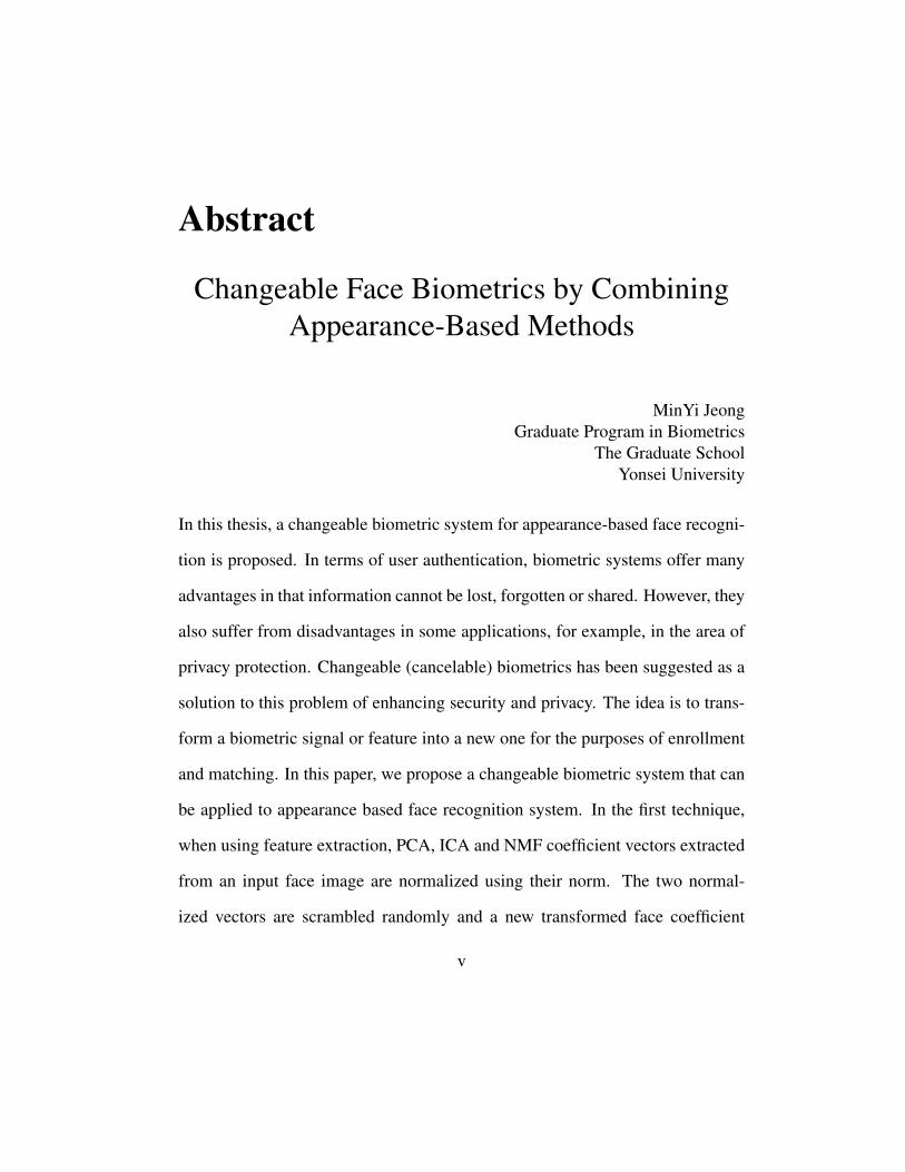
In this thesis, a changeable biometric system for appearance-based face recogni-

tion is proposed. In terms of user authentication, biometric systems offer many

advantages in that information cannot be lost, forgotten or shared. However, they

also suffer from disadvantages in some applications, for example, in the area of

privacy protection. Changeable (cancelable) biometrics has been suggested as a

solution to this problem of enhancing security and privacy. The idea is to trans-

form a biometric signal or feature into a new one for the purposes of enrollment

and matching. In this paper, we propose a changeable biometric system that can

be applied to appearance based face recognition system. In the first technique,

when using feature extraction, PCA, ICA and NMF coefficient vectors extracted

from an input face image are normalized using their norm. The two normal-

ized vectors are scrambled randomly and a new transformed face coefficient

v

vector (transformed template) is generated by addition of the two normalized

vectors. When this transformed template is compromised, it is replaced with a

new scrambling rule. Because the transformed template is generated by the ad-

dition of two vectors, the original PCA, ICA and NMF coefficients could not be

recovered from the transformed coefficients. In our experiments, we compared

performance when the PCA, ICA and NMF coefficient vectors is used and when

the transformed coefficient vectors are used for verification.

Key Words : biometrics, changeable biometrics, face recognition, princi-pal component analysis, independent component analysis, non-negative matrix factorization

vi

Chapter 1

Introduction

1.1 Biometrics

Biometric systems [1-3] refer to personal authentication methods that use indi-

vidual information from a given person such as fingerprints [4], face [5], iris

[6], palmprints [7], voice [8] or signature [9]. In the past years, the idea of

maintaining security by the use of passwords (knowledge-based security) and ID

cards (token-based security) has been used to restrict access to many applica-

tions. However, security can easily come under attack if a password is divulged

to an unauthorized user or an impostor. To prevent this, biometric systems have

emerged. These systems are believed to provide a greater degree of security than

traditional authentication methods. Among the many advantages of biometric

systems is the fact that most biometric information cannot be stolen, forgotten,

or shared. Biometric systems show many distinguished characteristics with re-

spect to the following points:

1. Universality, which means that each person must have the identified char-

1

acteristic.

2. Distinctiveness, which means that it must be easy to distinguish between

any two persons sufficiently in terms of the identified characteristic.

3. Permanence, which means that the identified characteristic must be fully

invariant over a given period of time.

4. Collectibility, which means that the identified characteristic can be mea-

sured quantitatively.

In a practical system which makes use of biometrics for personal identity

recognition, there are a number of other important requirements, as follows.

1. Performance, which refers to achievable identification accuracy, the re-

source requirements necessary to achieve acceptable identification accu-

racy, and the working or environmental factors that affect identification

accuracy.

2. Acceptability, which indicates to what extent people are willing to accept

a given biometric system.

3. Circumvention, which refers to how easy it is to fool the system by fraud-

ulent techniques.

A practical biometric system should meet the specified recognition accuracy,

speed, and resource requirements, be harmless to users, be accepted by the in-

tended population, and be sufficiently robust to various fraudulent attacks.

2

1.2 Changeable Biometrics

Although biometric systems offer many advantages for user authentication, there

are also some disadvantages. One of these is that there are privacy issues con-

cerning non-revocable biometric information, especially in cases of identity theft.

When a biometric template becomes compromised, it is rendered unusable. The

only remedy is to replace this template with another biometric feature. However,

a person has a limited number of biometric features, for example, the face, iris,

voice and hand. Changeable biometrics offers an alternative to these problems

[3]. Changeable biometrics refers to biometrics that can be changed canceled,

or replaced. These systems consist of an intentional, repeatable distortion of a

biometric signal based on a chosen transform. This transform can be applied

in either the signal domain or the feature domain. The biometric signal is then

changed in the same way at each presentation, for enrollment and for authentica-

tion. With this approach, every instance of enrollment can use a different trans-

form, thus rendering cross-matching impossible. Furthermore, if one variant of

the transformed biometric data is compromised, then the transform function can

simply be changed to create a new variant for re-enrollment. For changeable

biometric systems, there are five points to be considered.

The first point is that even if the biometric features are known, the original

biometrics cannot be recovered. This is called non-invertibility. Functions that

change the template have to be non-invertible transformations. An example of

this is changeable biometrics of the face and fingerprints [3]. The second point

3

is that after transformation, the recognition rate must not be much lower than

the original recognition rate. Ideally, the methods should provide better recogni-

tion rates. The third point is that transform functions can be created indefinitely.

Changeable biometric systems change because the number of biometrics is in-

sufficient. Therefore, the number of possible changed templates must be either

unlimited or numerous. This process is called reproducibility, and is calculated

through a measure of entropy. The fourth point is that the level of complexity

should be simple. It is not as necessary to satisfy this characteristic, but it is

needed as a changeable biometric performance measure. The fifth point is that

the changeable biometrics template has to look like a conventional biometric sys-

tem. Recently, research has been done on changeable biometric systems using

fingerprints [10], palmprints [11, 12], and faces [13-19].

1.3 Related Research

Several changeable biometrics methods have already been developed in the field

of face recognition. Ratha et al. [3, 13] proposed a morphing method to trans-

form face images. When the transformed biometric information was compro-

mised, a new biometric template was generated by introducing a new morphing

function. However, when using this method, it was still possible for the origi-

nal face image to be reconstructed if the attacker were to discover the morphing

function.

Savvides et al. [14] used random kernels and MACE (Minimum Average

4

Correlation Energy) filters. A transformed training image was created by con-

volving the given face image with a random kernel. The transformed image was

then used to generate the MACE filter. For authentication, a test image was

convolved with the same random kernel and this convolved test image was then

cross-correlated with the MACE filter.

Teoh et al. [15-18] proposed a method called BioHashing in which a feature

vector was projected onto a random vector basis and then scaled in a binary

way. The Fourier-Mellin transform and Fisher Discrimination Analysis (FDA)

were used for feature extraction. The feature vector was then calculated using

the extracted face feature, and the feature vector was projected onto a random

basis. Next, a random basis was found using the Gram-Schmidt procedure, with

a randomly generated vector set. Finally, a value of 0 or 1 was determined using

an arbitrary threshold. From the experimental results, this method was shown to

yield a zero EER.

However, contrary evidence was presented by Kong et al. [18], who showed

that the zero EER of the BioHashing method was produced under the impractical

assumption that the random basis can never be lost, stolen, shared or duplicated.

This assumption does not hold generally. Kong et al. also pointed out that if

this assumption held, there would be no need to use the random basis since it

could serve as a perfect password. Adopting an assumption generally used within

the biometric community, experimental results have since showed that the true

performance of BioHashing is far from perfect.

Kang et al. [19] proposed a changeable face biometric system which com-

5

bines the PCA template and a Password-Based Key Derivation Function (PBKDF).

In their method, authentication was performed in the permuted domain using a

permutation function which was created from a user’s password with the PBKDF.

If the transformed face template was compromised, a new face template was gen-

erated by alternating the password.

6

Chapter 2

Background

In this section, we give a brief related research about face recognition and change-

able biometrics for face recognition.

2.1 Face Recognition

Face-based systems [20] are very useful in many applications, since they are easy

to use, natural, and non-intrusive. A face recognition system generally consists

of four modules: detection, alignment, feature extraction, and matching.

Detection and alignment are processing steps that occur before feature ex-

traction and matching. The detection process separates the face areas from the

background, and alignment achieves accurate localization and normalization of

faces. Feature extraction is performed to provide information that is effective and

useful for distinguishing between the faces of different persons. Matching refers

to comparing the input face with faces in the database and deciding whether a

match is true or false. In a general sense, true means that the input face is equal

7

to a face in the database. For matching, the extracted feature vector of the input

face is matched against those of the enrolled faces in the database.

Face recognition can be further classified into two types: verification and

identification. Verification refers to a one-to-one match that compares a query

face image with a template face image. To evaluate performance, the verification

rate versus the false acceptance rate is calculated. This is called a Receiver Op-

eration Curve (ROC). A good verification system must try to balance these two

rates based on operational needs. Identification refers to a one-to-many matching

process that compares a query face image with all the template images in a face

database in order to determine the identity of the query face. Identification of

the test image is done by locating an image in the database which is most similar

to the test image. The test subject’s features are compared to the other features

in the system’s database and a similarity score is found for each comparison.

These similarity scores are then numerically ranked in descending order. The

percentage of times that the highest similarity score is the correct match for all

individuals is referred to as the top match score.

2.2 Appearance Based Method

Some typical algorithms for face recognition are presented below; namely, ap-

pearance based and model-based approaches. Appearance-based techniques have

been widely used in face recognition research [21-23]. These techniques repre-

sent a face as a linear combination of low-ranking basis images. They employ

8

Face detection

Face alignment

Featureextraction

Featurematching

Database of enrolled users

Face ID

Image/Video

Face location,size and pose

Aligned face

Feature extraction

Face detection

Face alignment

Featureextraction

Featurematching

Database of enrolled users

Face ID

Image/Video

Face location,size and pose

Aligned face

Feature extraction

Figure 2.1: Face recognition processing. A face recognition system generallyconsists of four modules as depicted in Figure 2.1 : detection, alignment, featureextraction, and matching.

9

feature vectors consisting of coefficients that are obtained by simply project-

ing facial images onto their basis images. Appearance-based approaches rep-

resent an object in terms of several object views. An image is considered to

be a high-dimension vector (a point in a high-dimensional vector space). Many

appearance-based approaches use statistical techniques to analyze the distribu-

tion of the object image vectors in the vector space, and derive an efficient and

effective representation according to different applications. Principal Compo-

nent Analysis (PCA), Independent Component Analysis (ICA) and Nonnegative

Matrix Factorization (NMF) are representative techniques for appearance-based

face recognition.

2.2.1 Principal Component Analysis

PCA [21-23] is a method which efficiently represents a collection of sample

data. Matthew A. Turk [21, 22] published a face recognition scheme that used

eigenfaces and was based on PCA. PCA is a way of identifying patterns, and ex-

pressing the identified information to highlight similarities and differences. PCA

is a method which efficiently represents a collection of sample information. The

eigenface algorithm uses PCA for dimensionality reduction in order to identify

the vectors which best account for the distribution of face images within the en-

tire image space. These vectors define the subspace of the face images. This

subspace is also called the face space. An eigenface is a face space that can be

obtained by analyzing sample face images with the PCA method, and it contains

features for identifying whether an acquired image is actually a face. In the PCA

10

method, the following equations are commonly used.

The training set of face images can be represented by Γ1, Γ2, ..., ΓM . The

average face of the training set is defined as Ψ = 1M

M∑n=1

Γn and different faces

are defined as Φi = Γi − Ψ . A covariance matrix can then be obtained in the

following way:

C =1

M

M∑n=1

ΦnΦTn . (2.1)

Each different face image Φi is represented as a linear combination of the eigen-

vectors. And each normalized training face Φk is represented by a vector Ωk =[wk

1 , wk2 , · · ·, wk

M ′]T .

Ωk = UT Φk. (2.2)

where, U = [u1u2 · · · u′M ] denotes the eigenvector for i = 1, ..., M ′ , and where

M ′ is the value that is found for face detection (M ′ ≤ M ).

Given an unknown face image Γ, it can be normalized and projected onto the

eigenspace.

Ω = UT (Γ−Ψ) . (2.3)

Similarly, all new face images can then be projected onto the face space to find

a set of weights that describe the contribution of each vector in the face space.

Fig. 2.2 shows facial image representations using PCA.

2.2.2 Independent Component Analysis

ICA [23-29] is an unsupervised learning rule that was derived from the principle

of optimal information transfer through sigmoidal neurons [30, 31]. ICA min-

11

Figure 2.2: Facial image representations using PCA.

imizes both second-order and higher-order dependencies in the input. It keeps

the assumption of linearity but abandons all the other aspects that PCA uses.

Although the amplitude spectrum is captured by second-order statistics in PCA,

there remains the phase spectrum that lies in higher-order statistics. ICA attempts

to find the basis along which the data (when projected onto them) are statistically

independent. ICA is a way of finding a linear non-orthogonal coordinate system

in any multivariate data. The directions of the axes of this coordinate system are

determined by both the second and higher order statistics of the original data.

The goal is to perform a linear transform, which makes the resulting variables as

statistically independent from each other as possible. This refers to a generaliza-

tion of PCA (therefore, PCA can be derived as a special case of ICA). The main

principle is to iteratively optimize a smoothing function whose global optima

occurs when the output vectors U are independent.

To define ICA, we considered a statistical model. We observed n random

variables x1, x2, · · · , xn, which were assumed to be linear combinations of n

unknown random variables s1, s2, · · · , sn. The independent components si were

latent variables, meaning that they could not be directly observed. We denoted

the observed variables xi as an observed vector x = [x1, x2, · · · , xn]T and the

12

Figure 2.3: Facial image representations using ICA.

component variables si as a vector s = [s1, s2, · · · , sn]T . The relation between s

and x was modeled as

x = As =n∑

i=1

aisi, (2.4)

where A is an unknown fixed n×n matrix of full rank, called the mixing matrix,

whose columns are denoted by ai, i = 1, · · · , n. Its columns were called the ICA

basis vectors or the ICA basis functions. Implementation of ICA was performed

to estimate the de-mixing matrix B, such that the vector x was transformed into

y = Bx (2.5)

yielding as mutually statistically independent components of y as possible.

The estimation of B is done by optimizing independence of the components in

y using training data. Thus, it is understood that the vector y is an estimate of

the true source s. There are two kinds of architectures based on ICA, statistically

independent basis images (architecture I) and a factorial code representation (ar-

chitecture II). In this paper, we used ICA architecture I. Fig. 2.3 shows facial

image representations using ICA.

13

2.2.3 Nonnegative Matrix Factorization

NMF is suggestive of some aspects of activation patterns in response to images.

In NMF, as the name implies, the amount of non-negativity adds constraints to

the matrix factorization, allowing only additions in the synthesis. There are no

cancellations or interference of patterns via subtraction or negative feature vector

values. This leads more naturally to the notion of parts-based representation of

images [32-34]. With the underlying non-negative constraints, NMF is able to

identify localized parts-based representations. Sparse coding with NMF seems

befitting especially for face recognition applications as the features of face im-

ages are naturally represented as a small collection of features, namely eyes,

nose and mouth, which are distributed all over the face. Because the outputs of

NMF are localized features, these parts-based features can be used collectively

to represent a face.

Given a data matrix F , non-negative matrix factorization refers to the decom-

position of the matrix F into two matrices W and H of size n × r and r × m,

such that

F = WH (2.6)

where the elements in W and H are all positive values.

In NMF, no negative entries are allowed in matrix factors W and H whereby

non-negativity constraint is imposed in factorizing the data matrix F limiting

data manipulation only to additions (no subtractions are allowed). This leads

to the idea of reconstructing an object by adding its representative parts collec-

14

tively. Each column in the matrix W is called a basis image, and a column in the

matrix H is called an encoding. An image in F can be reconstructed by linearly

combining basis images with the coefficients in an encoding. The encodings

influence the activation of pixels in the original matrix via basis images.

Given a data matrix F , Lee and Seung [33] developed a technique for factor-

izing the F to yield matrices W and H as given in Eq. (2.6). Each element in

the matrix F can be written as Fij =r∑

p=1

WipHpj where T represents the number

of basis images and the number of coefficients in an encoding. The following

iterative learning rules are used to find the linear decomposition:

Hpj ← Hpj

n∑i=1

(WipFij

r∑k=1

WikHkj

) (2.7)

Wip ← Wip

m∑j=1

(FijHpj

r∑k=1

WikHkj

) (2.8)

Wip ← Wipn∑

k=1

Wkp

(2.9)

The above unsupervised multiplicative learning rules are used iteratively to

update W and H . The initial values of W and H are fixed randomly. At each

iteration, a new value for W or H is evaluated. Each update consists of a multi-

plication and sums of positive factors.

The data matrix F , is constructed such that the training face images occupy

the columns of the F matrix. Let the training face set be Γtrain = f train1 , f train

2 , · · · , f trainm ,

F = [f1f2 · · · fm] and µ represents the mean of all training images. Learning is

15

1N × 1N+ × + 1N+ × 1N+ ×1N × 1N+ × + 1N+ × 1N+ ×1N × 1N+ × + 1N+ × 1N+ ×

Figure 2.4: Facial image representations using NMF.

done using Eq.s (2.7)-(2.9) to decompose the matrix F into 2 matrices, H and

W . Let the basis images be represented as W = [w1w2 · · ·wr] and encodings as

H = [h1h2 · · ·hm]: where each face fi in F can be approximately reconstructed

by linearly combining the basis images, and the corresponding encoding coeffi-

cients hTi = [h1ih2i · · ·hri] as shown in Figure 1. Hence: a face can be modeled

in terms of a linear superposition of basis functions together with encodings as

follows:

fi =r∑

j=1

wjhi (2.10)

For each face fi in the training set and test set, we calculate the corresponding

encoding coefficients. The basis images in W are generated from the set of

training faces;Γtrain. The encodings, hi of each training face fi is given by

hi = W †fi (2.11)

where W † is the pseudo-inverse of the matrix W . Once trained, the face image

set, f1, f2, · · · , fm is represented by a set of encodings h1, h2, · · · , hm with

reduced dimension, r. A distance metric is used to calculate the similarity be-

tween htraini and htest

j ; encodings of a training image and a test image. Fig. 2.4

shows facial image representations using NMF.

16

Chapter 3

Changeable Biometrics forAppearance-Based Methods

In this section, we describe the proposed method using appearance based method

for changeable face biometrics. The main idea of the proposed method is to gen-

erate transformed coefficients by addition of the coefficients of the scrambled

PCA and ICA coefficients (or the PCA and NMF) coefficients. In this section

Figure 3.1: Overall Procedure of Proposed Method.

17

the method using PCA and ICA is explained for the sake of convenience, but

other appearance method can be applied by same way. In the first technique,

the PCA and ICA coefficient vectors are extracted from an input face image and

normalized. The two normalized vectors are scrambled randomly and a new

transformed face coefficient vector is generated by addition of the two normal-

ized vectors. Fig. 3.1 shows the overall procedure of the proposed method.

3.1 Normalization

Using PCA and ICA algorithm, an n-dimensional PCA coefficient vector P = [P1,

P2, P3, ..., PN ] and ICA coefficient vector I = [I1, I2, I3, ..., IN ] are extracted from

an input face image, when the range of PCA and ICA coefficient vectors is very

different. Even though both coefficient vectors are added, the influencing power

of PCA is very large because the PCA coefficient vector is larger than the ICA.

When adding two vectors which are different from the influencing power, the

original face information can be disclosed if an attacker tries to use the coeffi-

cient vector of the large influencing power. Therefore, we have to consider the

influencing power of the PCA and ICA coefficient vectors. Therefore, the two

coefficient vectors are normalized using their norm as follows:

p = P/∣∣P

∣∣ = [p1,p2,p3,...,pN]

i = I/∣∣I

∣∣ = [i1,i2,i3,...,iN], (3.1)

where∣∣P

∣∣ and∣∣I

∣∣ denotes the L2 norm of vector P and I. Fig. 3.2 show the

distribution of the eigencoefficients before and after the proposed method.

18

-12000

-8000

-4000

0

4000

8000

12000

16000

20000

24000

28000

1 3 5 7 9 11 13 15 17 19 21 23 25 27 29 31 33 35 37 39

Dimension of coefficient

Val

ue

PCA coefficientICA coefficient

NMF coefficient

(a)

-0.05

-0.04

-0.03

-0.02

-0.01

0

0.01

0.02

0.03

0.04

0.05

0.06

1 3 5 7 9 11 13 15 17 19 21 23 25 27 29 31 33 35 37 39

Dimension of coefficient

Val

ue

Normalized PCA coefficient

Normalized ICA coefficient

Normalized NMF coefficient

(b)

Figure 3.2: Example of appearance based method eigencoefficients. (a) Exampleof PCA, ICA and NMF eigencoefficients. (b) Example of PCA, ICA and NMFnormalized eigencoefficients.

19

3.2 Scramble the normalized coefficient vector

To increase the reproducibility and complexity of non-invertiblity, we use a

scrambling method. The principal axes of the PCA and ICA vectors show a

large amount of information. By adding the arranged two vectors, the summa-

tion value is even larger. Therefore the principal axis is revealed easily. Attackers

would be able to obtain similar information as existed in the original one. The

principal axis of PCA and ICA is difficult to disclose using randomly scrambled

coefficient vectors.

This scrambling method is useful for the reproducibility of changeable bio-

metrics, since the number of possible changed templates must be unlimited or

numerous. The scrambling method exists in a large number of cases and con-

tributes to reproducibility. In this case, the number of cases is numerous because

each of the PCA and ICA vectors orders are differently scrambled and added.

Each coefficient vector is randomly scrambled and the scrambling rule is

determined by a user ID. It is possible to define the two scrambling functions

SPCAID (•) and ZICA

ID (•). SPCAID (•) is a function for scrambling the normalized PCA

coefficient vector p, and ZICAID (•) is a function for scrambling the normalized ICA

coefficient vector i. The scrambled PCA and ICA coefficient vectors are given

by;ps = SPCA

ID (p)

is = ZICAID (i)

(3.2)

When the transformed coefficient vector is found to be compromised, new trans-

formed coefficient vectors can be generated by replacing the user ID or the

20

scrambling rule associated with the user ID. In this way, many transformed face

coefficient vectors can be easily generated.

3.3 Addition between normalized coefficient vectors

Finally, the transformed face coefficient vector is generated by adding the scram-

bled PCA and ICA coefficient vectors as follows:

cID=∂ps+βis (3.3)

where ∂ = β = 1 in this paper.

One of the conditions for changeable biometrics is that transformed biomet-

ric data should not be easily converted back to the original biometric data even

if an attacker knows both the transformed biometric data and the transforming

method. In the proposed method, the information that an attacker can find is the

transformed face coefficient vector (cID=SPCAID (p)+ZICA

ID (i)) and the two scram-

bling functions (SPCAID (•),ZICA

ID (•)). However, because the PCA coefficient vec-

tor p and the ICA coefficient vector i are not stored, an attacker cannot dis-

cover the PCA coefficients nor the ICA coefficients (extra degree of freedom).

Therefore, it is impossible to recover the PCA and ICA coefficients from the

transformed coefficients cID. Therefore, this method satisfies the condition of

non-invertibility.

21

Chapter 4

Experiments

In this section, the experimental results are presented in three parts. In the first

part, we show how the performance rate varies when the number of dimensions

is changed from 10 to 300. Also, we compare performance when using PCA,

ICA (or PCA, NMF) and the proposed method. In the second part, we present

two experiments that address the changeability of changeable biometrics. The

first of these represents the changeability of the distribution of the eigencoeffi-

cients when using the proposed method, and the second represents changeability

through an system threshold and distribution of pseudo genuine elements. In the

last part, we calculate the amount of reproducibility.

4.1 Database

We used the AR Face database [35] to evaluate recognition performance. This

database consists of over 3,200 frontal view images of 126 subjects. There were

26 different images per subject, recorded in two different sessions separated by

22

Figure 4.1: Sample images from the AR Face database.

two weeks, each weekly session comprising 13 images. Each subject was cap-

tured under a large variety of conditions, including occlusion and changing facial

expressions. All images were obtained under controlled illumination and view-

point conditions. Each image consisted of a 46 by 56 array of pixels. We used

only 672 frontal facial images without occlusion and illumination changes, for a

total of 6 different images per subject. Fig. 4.1 shows some sample images taken

from the database. The number of images used for training and testing was both

336, respectively. The training set contained images for each of the 56 subjects.

The images of the remaining 56 subjects were used as the test set.

23

4.2 Experimental Design

4.2.1 Matching performance

Two samples of the same biometric feature from the same person can never be

exactly the same due to imperfect imaging conditions, ambient conditions, and

the user’s current state. A meaningful performance method is to use distance

distributions which show the distinctiveness and repeatability (consistency) of

the feature vectors transformed from the biometric signals. Genuine distribution

is created from the distance measures resulting from comparisons of a number

of face image pairs from the same face. Imposter distribution is created from the

distance measures generated by comparisons of a number of face images pairs

from different faces. The system decision is regulated by a threshold t. The

higher the score, the more certain it is that the two measurements come from the

same person.

A biometric verification system makes two types of errors: false rejections

and false acceptances[36]. These two types of errors are often termed as false

matches and false non-matches. False rejections refer to the likelihood (in trans-

action percentage terms) of an authorized user being wrongly rejected by the

system. False acceptances refer to the likelihood of an imposter being wrongly

rejected by the system. These two types of error usually have different costs as-

sociated with them, depending on the security requirements of the application. If

high security is the main goal, then the false acceptance rate (FAR) must be very

low. This can lead to a large false rejection rate (FRR) and potential user annoy-

24

ance. If user comfort with only mild security is the main goal, then a higher false

acceptance rate must be tolerated. Performance is often measured in terms of the

Equal Error Rate (EER), which is the point where the false acceptance rate and

the false rejection rate are approximately the same.

Fig. 4.2(a) graphically illustrates the computation of the FAR and the FRR

over genuine and imposter distributions. There is a strict tradeoff between FAR

and FRR in every biometric system. In fact, both the FAR and the FRR are

functions of the system threshold t. A ROC curve is used to report system per-

formance at all operating points (threshold t in Fig. 4.2(a)). A ROC curve is a

plot of FAR(t) against FRR(t) for various decision thresholds.

4.2.2 Changeability

Changeability means degree of deformation for transformed information accord-

ing to original information. If there are striking differences between the trans-

formed data and the original data, then the original information is better pro-

tected. For analysis, we used normalized eigencoefficient distribution to comply

with the original appearance-based method and the applied proposed method.

We also determined the degree of overlap by two distance distribution points

which were genuine versus before and after transformations. Fig. 4.3. show

genuine and imposter elements of normalized distance distribution and normal-

ized distance of the original eigencoefficients versus the transformed eigenco-

efficients by the proposed method for the same image. We defined the latter

distribution as ‘pseudo genuine distribution’. Also, we determined the threshold

25

Prob

abil

ity d

ensi

ty

distance

T

FRRFAR

Genuine distribution

Imposterdistribution

Prob

abil

ity d

ensi

ty

distance

T

FRRFAR

Genuine distribution

Imposterdistribution

(a)

Fals

e A

ccep

t Rat

e

False Reject Rate

•

•

•

t = T

Fals

e A

ccep

t Rat

e

False Reject Rate

•

•

•

t = T

(b)

Figure 4.2: The distance distributions: (a) genuine and imposter distribution, (b)a receiver operation curve (ROC).

26

Figure 4.3: The distance distributions: genuine, imposter, and pseudo genuinedistribution.

t as the EER point obtained by genuine and imposter distribution. If the distance

of the threshold t and the pseudo genuine distribution was further to the right,

the transformation before and after was more different. This is because the same

image of the before and after transformation was classified as an imposter. The

difference value means changeability by transformation. The degree of overlap

using the distribution of threshold t and the pseudo genuine element showed a

specific changeability value.

27

4.2.3 Reproducibility

Changeable biometric systems use change because the number of biometrics is

insufficient. Therefore, the transform functions can be created indefinitely and

the number of possible changed templates must be unlimited or numerous. This

is called reproducibility. For analysis of reproducibility, we calculated a number

of cases.

4.3 Experimental Results

4.3.1 Matching performance

We examined how the recognition rate varied when the number of dimensions

changed from 300 to 10. Within this framework, we compared performance

using PCA, ICAI(ICA architecture I), NMF and the proposed method. The ex-

perimental results of the proposed method were found for multiple instances for

each simulation because the scrambling function for the coefficients was a ran-

domly changing function. Therefore we conducted a total of 100 experiments

for each case, and used the Euclidian distance as a measurement of dissimilarity.

Fig. 4.4and Fig. 4.5 show the EER results when, firstly, the PCA coefficient

vector and the ICAI coefficient vector, and secondly, the PCA coefficient vector

and the NMF coefficient vector were used for verification, and when the trans-

formed coefficient vectors were used for verification, as the number of coefficient

dimension varied. These experimental results show that the EER of the proposed

method did not degrade significantly when using any of the conventional PCA,

28

10.00

12.00

14.00

16.00

18.00

20.00

22.00

24.00

26.00

28.00

10 30 50 70 90 110 130 150 170 190 210 230 250 270 290

Dimension

EE

R (

%)

PCA

ICA

Proposed method

Figure 4.4: Recognition performance of PCA, ICAI and proposed method invarying dimensions for the AR Face database.

ICAI, or NMF based methods.

4.3.2 Changeability

To establish the performance of the proposed method and its changeability, we

then confirmed the eigencoefficients. Fig. 4.6 and Fig. 4.7 show the distribution

of the eigencoefficients before and after using the proposed method. The original

face information was deformed when using the proposed method. Therefore, the

original face information was protected from an attacker because it is different

from the transformed eigencoefficients in the database.

The changeability value given by the number of 40 eigenfaces is shown in

Fig. 4.8 and Fig. 4.9 The results show the genuine and imposter elements of the

29

12.00

14.00

16.00

18.00

20.00

22.00

24.00

10 30 50 70 90 110 130 150 170 190 210 230 250 270 290

Dimension

EE

R (

%)

PCA

NMF

Proposed method

Figure 4.5: Recognition performance of PCA, NMF and proposed method invarying dimensions for the AR Face database.

normalized distance distribution to the applied proposed method and the pseudo

genuine distribution. We determined the threshold t as the EER point by using

the genuine and imposter distribution. All distribution was placed on the right

side rather than on threshold t. Namely, the same image of the before and af-

ter transformation was classified as an imposter element. These results mean

that the changeability for the proposed method was satisfying a good level of

changeability.

4.3.3 Reproducibility

Reproducibility was calculated by the number of cases of eigencoefficients pro-

duced by the scrambling rule. The scrambling method has large number of cases.

30

-0.05

-0.04

-0.03

-0.02

-0.01

0

0.01

0.02

0.03

0.04

0.05

1 3 5 7 9 11 13 15 17 19 21 23 25 27 29 31 33 35 37 39

Dimension of coefficient

Val

ue

Normalized PCA without scrambling

Normalized ICA without scrambling

Normalized (PCA + ICA) without scrambling

(a)

-0.05

-0.04

-0.03

-0.02

-0.01

0

0.01

0.02

0.03

0.04

0.05

1 3 5 7 9 11 13 15 17 19 21 23 25 27 29 31 33 35 37 39

Dimension of coefficient

Val

ue

Normalized PCA with scrambling

Normalized ICA with scrambling

Normalized (PCA + ICA) with scrambling

(b)

Figure 4.6: Example of PCA, ICAI and summation PCA and ICAI normalizedeigencoefficients. (a) Example of PCA, ICAI and summation PCA and ICAInormalized eigencoefficients without scrambling. (b) Example of PCA, ICAIand summation PCA and ICAI normalized eigencoefficients with scrambling.

31

-0.05

-0.04

-0.03

-0.02

-0.01

0

0.01

0.02

0.03

0.04

0.05

1 3 5 7 9 11 13 15 17 19 21 23 25 27 29 31 33 35 37 39

Dimension of coefficient

Val

ue

Normalized PCA without scrambling

Normalized NMF without scrambling

Normalized (PCA + NMF) without scrambling

(a)

-0.05

-0.04

-0.03

-0.02

-0.01

0

0.01

0.02

0.03

0.04

0.05

1 3 5 7 9 11 13 15 17 19 21 23 25 27 29 31 33 35 37 39

Dimension of coefficient

Val

ue

Normalized PCA with scrambling

Normalized NMF with scrambling

Normalized (PCA + NMF) with scrambling

(b)

Figure 4.7: Example of PCA, ICAI and summation PCA and ICAI normalizedeigencoefficients. (a) Example of PCA, NMF and summation PCA and NMFnormalized eigencoefficients without scrambling. (b) Example of PCA, NMFand summation PCA and NMF normalized eigencoefficients with scrambling.

32

0

0.1

0.2

0.3

0.4

0.5

0.6

0.7

0.8

0.9

1

0.0 0.1 0.2 0.3 0.4 0.5 0.6 0.7 0.8 0.9 1.0

Normalized distance

Nor

mal

ized

dis

trib

utio

n

Genuine

Imposter

Pseudo genuine

t0

0.1

0.2

0.3

0.4

0.5

0.6

0.7

0.8

0.9

1

0.0 0.1 0.2 0.3 0.4 0.5 0.6 0.7 0.8 0.9 1.0

Normalized distance

Nor

mal

ized

dis

trib

utio

n

Genuine

Imposter

Pseudo genuine

t

(a)

0

0.1

0.2

0.3

0.4

0.5

0.6

0.7

0.8

0.9

1

0 0.1 0.2 0.3 0.4 0.5 0.6 0.7 0.8 0.9 1

Normalized distance

Nor

mal

ized

dis

trib

utio

n

Genuine

Imposter

Pseudo genuine

t0

0.1

0.2

0.3

0.4

0.5

0.6

0.7

0.8

0.9

1

0 0.1 0.2 0.3 0.4 0.5 0.6 0.7 0.8 0.9 1

Normalized distance

Nor

mal

ized

dis

trib

utio

n

Genuine

Imposter

Pseudo genuine

t

(b)

Figure 4.8: Distribution of genuine, imposter and pseudo genuine elements. (a)PCA, Proposed method using PCA and ICAI. (b) ICAI, Proposed method usingPCA and ICAI.

33

0

0.1

0.2

0.3

0.4

0.5

0.6

0.7

0.8

0.9

1

0 0.1 0.2 0.3 0.4 0.5 0.6 0.7 0.8 0.9

Normalized distance

Nor

mal

ized

dis

trib

utio

n

Genuine

Imposter

Pseudo genuine

t0

0.1

0.2

0.3

0.4

0.5

0.6

0.7

0.8

0.9

1

0 0.1 0.2 0.3 0.4 0.5 0.6 0.7 0.8 0.9

Normalized distance

Nor

mal

ized

dis

trib

utio

n

Genuine

Imposter

Pseudo genuine

t

(a)

0

0.1

0.2

0.3

0.4

0.5

0.6

0.7

0.8

0.9

1

0 0.1 0.2 0.3 0.4 0.5 0.6 0.7 0.8 0.9

Normalized distance

Nor

mal

ized

dis

trib

utio

n

Genuine

Imposter

Pseudo genuine

t0

0.1

0.2

0.3

0.4

0.5

0.6

0.7

0.8

0.9

1

0 0.1 0.2 0.3 0.4 0.5 0.6 0.7 0.8 0.9

Normalized distance

Nor

mal

ized

dis

trib

utio

n

Genuine

Imposter

Pseudo genuine

t

(b)

Figure 4.9: Distribution of genuine, imposter and pseudo genuine elements. (a)PCA, Proposed method using PCA and NMF. (b) NMF, Proposed method usingPCA and NMF.

34

If number of n was chosen as the dimension of used eigenfaces, the number of

cases for an n eigenface scrambling method was n!. Here, the number of cases

was numerous because the order of each of the PCA and ICAI (or PCA and

NMF) vectors was differently scrambled and added. Therefore, the total number

of cases for the proposed method was n! × n! obtained by using a differently

randomly scrambled method. For example, if we used 50 eigenfaces (n), we

had 50!× 50! = 9.2502e + 128 cases for reproducibility. Therefore, this method

contributed to reproducibility, which is good for changeable biometric systems.

35

Chapter 5

Conclusions

Biometrics is a method of personal authentication. Among its many advantages

is the fact that information cannot be stolen, forgotten, or shared. Also, biometric

systems provide a greater degree of security compared with traditional authen-

tication methods. However, there are also weak points. One of these problems

is the issue of privacy concerning non-revocable biometrics, especially in the

case of identity theft. When a biometric template is compromised, it is rendered

unusable because biometric data cannot be discarded and reissued. The only

remedy is to replace the template with another biometric feature. However, a

person has only a limited number of biometric features. Moreover, if biometric

templates get stolen, an attacker can attack other authentication systems by us-

ing the compromised biometric templates. The key reason for these drawbacks

is that biometric information is derived from a person’s physical features, and

thus, biometrics cannot be as easily changed as password or keys.

Changeable biometrics is an alternative to biometric problems. It uses trans-

formed or distorted biometric data instead of original biometric data for identi-

36

fying a person. When a set of biometric data is found to be compromised, it can

be discarded and a new set can be generated.

In this thesis, we proposed a changeable biometric system for face recogni-

tion using an appearance-based approach. The main idea was to scramble the

PCA and ICA (or the PCA and NMF) coefficient vectors and find a weighted

sum of the two vectors. From experimental results, it is clear that this method can

maintain performance comparable to that of conventional methods. By scram-

bling the order of the coefficients in the transform function, we were able to

generate numerous instances of changeable face data. Therefore, the proposed

method is characterized by not only resolving a weak point of biometric systems,

but also maintaining good performance.

37

Bibliography

[1] A.K.Jain,R.Bolle, and S. Pankanti, BIOMETRICS: Personal Identification in

Networked Society, Kluwer Academics Publishers, Norwel, MA, 1999.

[2] A.Pankanti,R.M.Bolle, and A.K.Jain, “Biometrics: the future of identifica-

tion,” IEEE Computer, Vol.33, No.2, pp.46-49, 2000.

[3] N. K. Ratha, J. H. Connell, and R. M. Bolle, “Enhancing security and privacy

in biometrics-based authentication systems,” IBM Systems Journal, Vol. 40,

No. 3, 2001.

[4] D. Maltoni, D. Maio, A. Jain, and S. Prabhaker, Handbook of Fingerprint

Recognition, Springer, 2003.

[5] R. Chellappa, C.L. Wilson, S. Sirohey, “Human and machine recognition of

faces: a survey,” Proceedings of the IEEE, vol.83, no.5, pp.705-741, 1995.

[6] M. Negin, T. Chmielewski Jr., M. Salganicoff, T. Camus, M. Seelen, L.

Venetianer, and G. Zhang, “An Iris Biometric System for Public and Per-

sonal Use,” IEEE Computer, vol.3, no.2, pp.70-75, 2000.

38

[7] Chih-Lung Lin and Kuo-Chin Fan, “Biometric verification using thermal im-

ages of palm-dorsa vein patterns,” IEEE Transactions on Circuits and Sys-

tems for Video Technology, vol.14, No.2, pp.199 - 213, 2004.

[8] J. Naik, “Speaker verification: a tutorial,” IEEE Communications Magazine,

vol.28, No.1, pp.42-48, 1990.

[9] Jonghyon Yi, Chulhan Lee, and Jaihie Kim, “Online signature verification

using temporal shift estimated by the phase of Gabor filter,” IEEE Transac-

tions on Signal Processing, vol.53, no.2, pp.776 - 783, 2005.

[10] R. Ang, R. Safavi-Naini and L. McAven, “Cancelable Key-Based Finger-

print Templates,” Australasian Conference on Information Security and Pri-

vacy, 2005, LNCS 3574, pp. 242-252, 2005.

[11] T. Connie, A. Teoh, M. Goh and D. Ngo, “PalmHashing: a novel approach

for cancelable biometrics,” Information Processing Letters 93, pp. 1-5, 2005.

[12] Y. Pang, A. Teoh and D. Ngo, “Personal Authenticator on the Basic of

Two-Factors: Palmprint Features and Tokenized Random Data,” Artificial

Intelligence 2004, LNAI 3339, pp. 227-236, 2004.

[13] R. M. Bolle, J.H. Connel, N.K. Ratha, “Biometrics Perils and Patches,”

Pattern Recognition, Vol. 35, pp. 2727-2738, 2002

39

[14] M. Savvides, B. V. K Vijaya Kumar and P. K. Khosla, “Cancelable Bio-

metric Filters for Face Recognition,” Proceedings of the 17th International

Conference on Pattern Recognition (ICPR 2004), pp. 922-925, 2004.

[15] A. Teoh, D. Ngo and A. Goh, “An Integrated Dual Factor Authenticator

Based on the Face Data and Tokenised Random Number,” International

Conference on Bioinformatics and its Applications 2004, LNCS 3072, pp.

117-123, 2004.

[16] A. B. J. Teoh, D. C. L. Ngo and A. Goh, “Personalised cryptographic key

generation based on FaceHashing,” Computers and Security, Vol. 23, No. 7,

pp. 606-614, 2004.

[17] A. B. J. Teoh and D. C. L. Ngo, “Cancelable biometrics featuring with

tokenized random number,” Pattern Recognition Letter, Vol. 26, No. 10, pp.

1454-1460, 2005.

[18] A. Kong, K. H. Cheung, D. Zhang, M. Kamel, and J. You, “An analysis of

BioHashing and its variants,” Pattern Recognition, 27 December, 2005.

[19] J. Kang, D. Nyang, and K. Lee, “Two Factor Face Authentication Scheme

with Cancelable Feature,” International Workshop on Biometric Recognition

Systems (IWBRS), pp. 67-76, 2005.

[20] Stan Z. Li and Anil K. Jain, Handbook of Face Recognition, Springer, 2003.

40

[21] M. A. Turk and A. P. Pentland, “Eigenfaces for recognition,” Cognitive

Neuroscience, Vol. 3, No. 1, pp. 71-86, 1991.

[22] M. A. Turk and A. P. Pentland, “Face Recognition Using Eigenfaces,” Com-

puter Vision and Pattern Recognition, 1991, Proceedings CVPR ’91, IEEE

Computer Society Conference on 3-6, pp. 586-591, 1991.

[23] B. A. Draper, K. Baek, M. S. Bartlett, and J.R. Beveridge, “Recognizing

faces with PCA and ICA,” Computer vision and image understanding, spe-

cial issue on Face Recognition, pp. 115-137, 2003.

[24] A. Hyvarinen, J. Karhunen, and E. Oja, Independent Component Analysis,

Wiley, 2001.

[25] Pong C. Yuen and J.H.Lai, “Face Representation Using Independent Com-

ponent Analysis,” Pattern Recognition, Vol. 35, No. 6, pp. 1247-1257, 2002.

[26] M. Bressan, D. Guillamet, and J. Vitria, “Using an ICA Representation of

Local Color Histograms for Object Recognition,” Pattern Recognition, Vol.

36, No. 3, pp. 691-701, 2003.

[27] R.Jenssen and T.Eltoft, “Independent Component Analysis for Texture seg-

mentation,” Pattern Recognition, Vol. 36, No. 10, pp. 2301-2315, 2003.

[28] Te-Won Lee and Lewicki M.S., “Unsupervised image classification, seg-

mentation, and enhancement using ICA mixture models,” IEEE Transactions

on Image Processing, Vol. 11, No. 3, pp. 270-279, 2002.

41

[29] S. Noh, “Iris Recognition System Based on Independent Component

Analysis”, Ph.D thesis, Yonsei University, 2005.

[30] A.J. Bell and T.J. Sejnowski, “An information-maximization approach to

blind separation and blind deconvolution,” Neural Computation, pp.1129-

1159, 1995.

[31] S. Laughlin. “A simple coding procedure enhances a neuron’s information

capacity,” Z. Naturforsch, pp. 910-912, 1981.

[32] M. Rajapakse and L. Wyse, “NMF vs ICA for face recognition”, in Pro-

ceedings of the 3rd International Symposium on Image and Signal Process-

ing and Analysis (ISPA ’03), vol. 2, pp. 605-610, Rome, Italy, September

2003.

[33] Daiel, D. Lee, and H. Sebastian Seung, “Learning the parts of objects by

non-negative matrix factorization”, Nature, Vol.401, pp. 788-791, 1999.

[34] Daiel, D. Lee, and H. Sebastian Seung, “Algorithms for Non-negative Ma-

trix Factorization”, Proc. Neural Information Processing Systems, 2000.

[35] A. M. Martinez and R. Benavente, “The AR Face Database,” CVC Tech,

1998.

[36] R.O. Duda, P.E. Hart, G. Stork, Pattern Classification, second ed., Wiley,

New York, 2000.

42

²DGëH¹כ

ü@+þAlìøÍlZO_½+Ë$í\_ôÇ\OÏãJÒqtd

s7HëH\"fHÒqtd¦s6 xôÇ>h7£xr±úúeHáÔs

!QrëH]j_K¦0A #\OÏãJd¦0AôÇÒqtd¦]jîßôÇ.

ÒqtdÉr >h_ 1lq:£¤ôÇ Òqt&ñÐ\¦ 6 x # 7£x¦ H ~½ÓZO ×æ

Ð&ñÐ\¦6 x Ù¼Ð~1> èß©½+Éú\OH&h,Êë@/_Ô¦¼#

<Ês\OH&h,9#Q!Qot·ú§HH&h,/BNÄ»½+Éú\OH&h1px ú§Ér©

&hse.ÕªQÒqt:£¤$íÉrժúôÇ&ñ÷&#QelM:ëH\ èß©

<H©¦©Ùþ¡¦âĺâsÔ¦0px ÕªSúBĺ]jôÇ)a.

ÒqtdÉrsÒqtdëH]j\¦K l0AôÇ@/îß×æ s.

ÒqtdÉrâ0pxôÇÒqtdlZOܼÐ+$©)aÒqt&ñÐ\ëH]j

µ1ÏÒqt 1px2¤÷&#Qe~Òqt&ñÐ\¦2[è ¦ÉrÒqt&ñÐÐâ

#6 x½+Éúe6£§¦_pôÇ.Òqtd¦0AK"fH$8<Êú

\¦ ×þ # Òqt&ñÐ\¦ +þA rv¦, +þA)a Òqt&ñÐ\¦ z]j rÛ¼%7¦

0AôÇÒqt&ñÐÐ6 x >)a.s8<ÊúH|ÃÐ\ ¢HrÛ¼%7

\ØÔ>ÅÒ#Qt 9,ëßÒqt&ñÐ èߦ©Ùþ¡¦âĺl>r_Òqt

&ñÐH ]j\¦ ¦ DhÐîr 8 <Êú\¦ ½+É© ~ÃÎ DhÐîr Òqt&ñÐ\¦

r Òqt$í > )a. sM: â)a <ÊúРëß[þt#Q Òqt&ñÐH s_ Òqt

&ñÐü<)©'a$ís\Oܼ 9"é¶:r%ò©Ü¼Ð4¤½ H Ô¦0pxכ.

43

ĺoH l>r\ ·ú9 \OÏãJd_ ~½ÓZO îrX< ü@+þA lìøÍ l

ZO(appea-rance-based method)_¦Ä»>ú(eigencoefficient)\¦s6 x #

Òqtd¦ ½&³ H ~½ÓZO¦ ]jîßôÇ. $ ôÇ %ò©\"f "fÐ Ér ü@+þA

lìøÍlZO¦s6 x #¦Ä»>ú\¦ÆÒئôÇ.ÆÒئ)ay¦Ä»>ú°ú#3_כ

0A\¦ îïro(normalization) :x # 9ur. îïro )a yy_ ¦Ä»>

ú\¦½ ü<Êú\¦s6 x #Ô¦½©gË: >íH"f\¦âôÇ.e_&hܼÐíH"f

FC\P)a ¦Ä»>ú\¦ "fÐ 8ôÇ. sXO> 8K4R Òqt$í)a +þA ¦Ä»>

ú\¦ d\ 6 xôÇ. ]jîß)a \OÏãJ Òqt&ñÐ Òqt$í ~½ÓZOÉr yy_ ¦Ä»>

ú_ íH"f\¦ e_Ð â # ÁºôÇôÇ \OÏãJ &ñÐ\¦ Òqt$í½+É Ãº e2¤

%i¦¦Ä»>ú\¦8<ÊܼÐ+q%i$í(non-invertibility)¦ëß7á¤rv9¦

rÙþ¡.

]jîß)a~½ÓZO¦s6 xôÇz+«>õ\OÏãJÒqt&ñÐ\¦6 xK >h

7£x_$í0pxsÄ»tHd¦SX½+Éúe%3.+þA)a¦Ä»>ú[þtÉr"鶦Ļ

>ú[þt_°úכõBĺØÔÙ¼Ð"é¶&ñÐ_Ð ñl0px¦. ¢ôÇs~½ÓZO

Ér îïroü< 8 l íߦ '¬Il M:ëH\ %i8s Ô¦0px ¦, íH"f

â¦0Aôǽ ü<ÊúÁºôÇ Ù¼ÐFÒqtíß$í¦Øæìryëß7á¤rv 9,gË:

íßëߦ s6 x ټР>íßs çßéß . > 4¤"é¶)a %ò©Ér "é¶:rõ Bĺ

ØÔÙ¼Ð>h\OÏãJ&ñÐ\¦Ð ñ½+Éúe."f]jîß~½ÓZOÉrÒqt

d\Bĺ&h½+Ë .

Ùþd÷&H ú :Òqtd, Òqtd, \OÏãJ d, ÅÒ$íìr ìr$3, 1lqwn $íìrìr$3,q6£§Ãº ½5Åq|¦Ér'§>=ìrK

44