
CHALMERS UNIVERSITY OF TECHNOLOGY DEPARTMENT OF …
160
SE0500189 Development and Investigation of Reactivity Measurement Methods in Subcritical Cores Johanna Wright CHALMERS UNIVERSITY OF TECHNOLOGY DEPARTMENT OF REACTOR PHYSICS ISSN 0281-9775
Transcript of CHALMERS UNIVERSITY OF TECHNOLOGY DEPARTMENT OF …

SE0500189
Development and Investigation of
Reactivity Measurement Methodsin Subcritical Cores
Johanna Wright
CHALMERS UNIVERSITY OF TECHNOLOGY
DEPARTMENT OF REACTOR PHYSICS
ISSN 0281-9775

CHALMERS
Development and Investigation of Reactivity
Measurement Methods in Subcritical Cores
Johanna Wright
Licentiatuppsats som presenteras vid ett seminariummandagen den 30 ma j 2005, k l . 10.30, i sal FL52,
Origohuset, Chalmers Tekniska Hogskola
Uppsatsen finns tillganglig vidAvdelningen for Reaktorfysik
Chalmers University of Technology412 96 Goteborg,
Telefon 031-772 1000

Development and Investigation of Reactivity Measurement Methods inSubcritical Cores
Johanna WrightDepartment of Reactor Physics
Chalmers University of TechnologySE-412 96 Goteborg, Sweden
Abstract
Subcriticality measurements during core loading and in future acceleratordriven systems have a clear safety relevance. In this thesis two subcriticalitymethods are treated: the Feynman-alpha and the source modulation method.
The Feynman-alpha method is a technique to determine the reactivityfrom the relative variance of the detector counts during a measurement pe-riod. The period length is varied to get the full time dependence of thevariance-to-mean. The corresponding theoretical formula was known onlywith stationary sources. In this thesis, due to its relevance for novel reactiv-ity measurement methods, the Feynman-alpha formulae for pulsed sourcesfor both the stochastic and the deterministic cases are treated. Formulaeneglecting as well as including the delayed neutrons are derived. The formu-lae neglecting delayed neutrons are experimentally verified with quite goodagreement.
The second reactivity measurement technique investigated in this thesisis the so-called source modulation technique. The theory of the method waselaborated on the assumption of point kinetics, but in practice the methodwill be applied by using the signal from a single local neutron detector. Ap-plicability of the method therefore assumes point kinetic behaviour of thecore. Hence, first the conditions of the point kinetic behaviour of subcriticalcores was investigated. After that the performance of the source modulationtechnique in the general case as well as and in the limit of exact point ki-netic behaviour was examined. We obtained the unexpected result that themethod has a finite, non-negligible error even in the limit of point kinetic be-haviour, and a substantial error in the operation range of future accelaratordriven subcritical reactors (ADS). In practice therefore the method needs tobe calibrated by some other method for on-line applications.
Keywords: reactivity measurement, subcritical cores, core loading, Accel-erator Driven Systems (ADS), Feynman-alpha formulae, source modulationmethod, point kinetic
THESIS FOR THE DEGREE OF LICENTIATE OF ENGINEERING CTH-RF-190
Development and Investigation of
Reactivity Measurement Methods
in Subcritical Cores
Johanna Wright
Akademisk uppsats for avlaggande avteknologie licentiatexamen i Reaktorfysik
vid Chalmers Tekniska Hogskola
Examinator och handledare: Professor Imre PazsitGranskare: Dr. Vasily Arzhanov, KTH
Department of Reactor PhysicsChalmers University of Technology
Goteborg, Sweden, May 2005


Development and Investigation of Reactivity Measurement Methods inSubcritical Cores
Johanna WrightDepartment of Reactor Physics
Chalmers University of TechnologySE-412 96 Goteborg, Sweden
Abstract
Subcriticality measurements during core loading and in future accelerator drivensystems have a clear safety relevance. In this thesis two subcriticality methods aretreated: the Feynman-alpha and the source modulation method.
The Feynman-alpha method is a technique to determine the reactivity from therelative variance of the detector counts during a measurement period. The period lengthis varied to get the full time dependence of the variance-to-mean. The correspondingtheoretical formula was known only with stationary sources. In this thesis, due to itsrelevance for novel reactivity measurement methods, the Feynman-alpha formulae forpulsed sources for both the stochastic and the deterministic cases are treated. Formulaeneglecting as well as including the delayed neutrons are derived. The formulae neglectingdelayed neutrons are experimentally verified with quite good agreement.
The second reactivity measurement technique investigated in this thesis is the so-called source modulation technique. The theory of the method was elaborated on theassumption of point kinetics, but in practice the method will be applied by using thesignal from a single local neutron detector. Applicability of the method therefore as-sumes point kinetic behaviour of the core. Hence, first the conditions of the point kineticbehaviour of subcritical cores was investigated. After that the performance of the sourcemodulation technique in the general case as well as and in the limit of exact point kineticbehaviour was examined. We obtained the unexpected result that the method has afinite, non-negligible error even in the limit of point kinetic behaviour, and a substantialerror in the operation range of future accelarator driven subcritical reactors (ADS). Inpractice therefore the method needs to be calibrated by some other method for on-lineapplications.
Keywords: reactivity measurement, subcritical cores, core loading, Accelerator DrivenSystems (ADS), Feynman-alpha formulae, source modulation method, point kinetic

This licentiate thesis consists of an introductory text and the following four appendedresearch papers, henceforth referred to as PAPER I, PAPER II, PAPER III, and PAPERIV.
I. J. Wright and I. Pazsit, Derivation and analysis of the Feynman-alpha formulafor deterministically pulsed sources,CTH-RF-179, 2004, Chalmers University of Technology, Goteborg, Sweden
II. I. Pazsit, Y. Kitamura, J. Wright and T. Misawa, Calculation of the pulsed Feynman-alpha formulae and their experimental verification,Annals of Nuclear Energy, 32, pp.986-1007 (2005)
III. Y. Kitamura, I. Pazsit, J. Wright, A. Yamamoto and Y. Yamane, Calculation ofthe pulsed Feynman-and Rossi-alpha formulae with delayed neutrons,Annals of Nuclear Energy, 32, pp.671-692 (2005)
IV. J. Wright and I. Pazsit, Neutron kinetics in subcritical cores with application tothe source modulation method,Submitted to Annals of Nuclear Energy (2005)


Acknowledgements
First and foremost, I would like to thank my supervisor Professor Imre Pazsit for alwaysanswering my many questions, supporting me, and providing me with the interestingproblems. Also, I would thank Dr. Yasunori Kitamura for the co-operation on thework connected with this thesis. I would also thank Carl Sunde and Johan Staring forpatiently reading the proof and giving helpful comments. Furthermore, I would thankall my colleagues at the Department of Reactor Physics.
Swedish Centre for Nuclear Technology (Svenskt Karntekniskt Centrum, SKC) is grate-fully acknowledged for the financial support.
Goteborg, Spring 2005
Johanna Wright
VII


Contents
1 Introduction 1
2 Reactivity Measurement Methods 32.1 Feynman-alpha method 32.2 Rossi-alpha method 42.3 Source modulation method 52.4 Break frequency noise analysis method 52.5 Californium-252 method 6
3 Pulsed Feynman-alpha Formulae 93.1 Feynman-alpha formula neglecting delayed neutrons 9
3.1.1 Deterministic pulsing 113.1.2 Stochastic pulsing 14
3.2 Feynman-alpha formula including delayed neutrons 163.2.1 Deterministic pulsing 183.2.2 Stochastic pulsing 20
4 Source Modulation Method 214.1 Kinetics of subcritical cores 21
4.1.1 Point reactor approximation 234.1.2 Kinetics of subcritical cores with a source 23
4.2 Analysis of the performance of the source modulation method 25
4.3 Possible methods for improving the performance 28
5 Concluding remarks 31
Bibliography 33
Abbreviations 37
Paper I-IV 39
IX

1Introduction
Reactivity measurements are important both in power reactors as well as in futuresource-driven subcritical systems. Recently, the topic has received new actuality dueto a few incidents such as in Tokaimura in 1999 [1-3] or at Dampierre in 2001 [4]. InTokaimura a criticality accident occurred at a uranium conversion facility, when severaltimes more than the specified limit of a solution of enriched uranium had been added ina precipitation tank until the critical mass was achieved, resulting in a self-sustainingnuclear fission chain reaction [3]. Unfortunately, three workers suffered acute radiationsyndrome and several workers as well as members of the public received radiation doses.The incident in France happened during a routine refuelling of the Dampierre-4 PWR,where one fuel assembly was skipped by mistake when the work shift changed. Whenthe error was noticed near the end of the refuelling sequence, the core configurationwas quite different from that intended due to the fact that 113 fuel assemblies wereincorrectly positioned [4]. Under unfavourable circumstances this could have resultedin prompt criticality.
The two examples above illustrate the renewed actuality of subcriticality measure-ments. In particular, there are two major areas of interest; core loading in power reactorsand future Accelerator Driven Systems (ADS). Today there are no satisfactory methodsfor reactivity measurements and monitoring during core loading. In general, the avail-able systems use a Start-up and Intermediate Monitors (SIRM) system that causes areactor shut down or scram if the amplitude of the neutron flux or the increase rate ofthe flux becomes larger than empirical limits. If the core configuration is unfavourable,it can lead to prompt criticality. Under such circumstances the SIRM system is notenough and it is necessary to measure criticality during core loading to avoid a config-uration that leads to an unexpected event. As is seen in the case at Dampierre it ispossible to load a large number of fuel elements incorrectly. However, for a BWR only30 misplaced fuel elements can lead to prompt criticality [5].
Recently, ADS has received increased interest, since it is a promising system fornuclear waste transmutation. An ADS is a non-self-sustaining subcritical reactor drivenby a strong external neutron source. Some experimental programs are being performedto develop such systems [6-8]. As the experimental programs also underline, on-linemonitoring of the subcritical reactivity is one of the central operational and safety issuesof a future ADS. The reason is that the reactivity variations under no circumstancesshould lead neither to criticality nor delayed criticality. In the EU project MUSE, a largenumber of reactivity measurement methods applicable in zero or low power systems, suchas the Feynman- and the Rossi-alpha methods, and pulse decay methods, including thearea ratio method of Sjostrand [9] were investigated. However, it is obvious that at thehigher operating level of a power producing ADS, zero noise methods need to be replacedby other ones, just as in an operating critical reactor inverse kinetic methods are used
1

Chapter 1 Introduction
for reactivity measurements instead of the Feynman-alpha or pulse decay methods.There are several similarities between the subcriticality measurements during core
loading and in ADS. To measure reactivity during core loading one needs an externalsource analogous to the driving source in ADS. In addition, since both systems aresubcritical, their neutron kinetic characteristics are similar. Therefore, similar reactivitymeasurement techniques can be used for both cases.
The outline of this thesis is as follows: Chapter 2 is a continuation of the introduc-tion with an overview of the common subcriticality measurement methods. In Chapter3 a derivation of the Feynman-alpha formulae for pulsed sources is given. We treatthe stochastic as well as the deterministic pulsing and even include delayed neutrons.Further, in Chapter 4 the so-called source modulation technique for reactivity mea-surement in subcritical cores is investigated. In Chapter 5, finally, concluding remarksare made.
The thesis also contains four appended papers. PAPER I, PAPER II, and PAPER
III deal with the pulsed Feynman-alpha formulae. PAPER IV is an investigation ofthe source modulation method including a revision of the conditions of point kineticbehaviour in subcritical cores. PAPER III also includes a derivation of pulsed Rossi-alpha formulae, omitted in this thesis.

2Reactivity Measurement Methods
There is a number of methods for conventional subcriticality measurements. Here, ashort description of the Feynman-alpha, the Rossi-alpha, the source modulation, thebreak frequency noise analysis, and the Cf-252 methods are given. Both the Feynman-and Rossi-alpha methods are based on neutron fluctuations and the measurement of thesecond moment of the statistics of the detector counts. The break frequency and theCf-252 methods are based on measurements of auto-power and/or cross-power spectraldensities. However, the basis of all these methods is that the statistical propertiesof the count sequence depend on the dynamic properties of the multiplying system.The methods that use a single detector are based on the assumption of point kineticbehaviour of the system.
2.1 Feynman-alpha method
The Feynman-alpha method, also called variance-to-mean method, is based on the mea-surement of the relative variance of the detected neutron counts as a function of themeasurement time t [10,11]:
where Z(t) is the detector counts, (Z(t)) its expectation value, and o1(t) is the varianceof Z. In practice, one uses an external neutron source and repeatedly detects the numberof detector counts during a time interval t. The measurement interval is varied and foreach interval the mean and the variance are determined.
Assume both an infinite reactor and detector, and a Poisson source, i.e. the proba-bility to emit one neutron in dt being Sdt. Then, using the master equation formalismfor the probability distributions the Feynman-alpha formula is obtained [12] as
°M ^ , (, i-«-°'r
where e is the detection efficiency.For the prompt part of the sum, i.e. i = 0, which includes the reactivity and is thus
the most important part, the following relationships are given:
ft - p k - la0 « ——-, p - —j—, OLi < a0; i > 1 (2.3)
and
Ao~ & (/3P)2-(^T ( 2-4 )

Chapter 2 Reactivity Measurement Methods
where a0 is the prompt neutron decay constant, /? is the delayed neutron fraction, p thesubcritical reactivity, and A the prompt neutron generation time. Further, D is averagetotal number of neutrons per fission, (v(v — 1)) is the second-order factorial momentof total number of neutrons generated per fission, and Dv is the fission Diven factor,denned as
D. = **£i». (2.5)Obviously, the interesting information is contained in the deviation of the relative
variance from unity, i.e. in the Feynman V-function
Y(t) -(z(t))
whereHz(t) = o2
z(t) - (Z(t)) = (Z(t)(Z - 1)) - (Z(t))2 (2.7)
is called the modified variance. The reason is that if all neutrons were statisticallyindependent, as those emitted by a radioactive source, they would have Poisson statisticsand the relative variance in eq. (2.2) would equal unity. In other words, we would notgain any information in the system. In a multiplying medium, however, each neutroninduces a chain of correlated neutrons. Positive correlations lead to a variance higherthan Poisson and it is the part that is larger than unity that contains the useful systeminformation. In a subcritical reactor each individual chain will die out exponentiallywith the time constants at, hence the relative variance will saturate.
The parameter c*o is obtained by curve fitting to experimental data and then thereactivity can be calculated using eqs. (2.3), which does not require knowledge of thedetector efficiency or the source strength.
2.2 Rossi-alpha method
The Rossi-alpha method (Orndoff's type), also called the correlation or covariancemethod, is based on the measurement of the covariance function of the detector countsin infinitesimal time intervals dt around two different times t and t + r [13]. Assuminga Poisson source, i.e. the probability to emit one neutron in dt being Sdt, the Rossiformula is often written as
where CZZ(T) is the stationary value of the covariance function, Z(t) and Z(t + r) are thedetector counts during dt around t and t + r, respectively, and (Z(t)) and (Z(t + r)) arethe first moments of the stationary detector counts in (t, dt) and (t + r, dt), respectively.Because of the stationarity, the quantities depend not on t, but on r.
Using the master equations, an analytical expression for the covariance can be de-rived:
6
P{r)dr = edr ^ C.e'^, (2.9)t=0

2.3 Source modulation method
where the d are similar to Ai and the other parameters are the same as in eq. (2.6).If all the neutrons were independent, the covariance would be zero. Since the neutronsgenerated by fission are correlated, the covariance becomes larger than zero. Similarlyto the Feynman formula, the neutron chains will die out with the same time constants.Again, the parameter aQ and the reactivity is obtained by curve fitting to experimentaldata.
2.3 Source modulation method
The source modulation method is proposed by Carta and D'Angelo [14] for subcriticalitymonitoring in ADS. However, the method could be used during core loading as well.The idea of source modulation method is that by varying the amplitude of the externalsource neutron fluctuations are induced. Using the point kinetic equations, for suchfluctuations the following relationship can be derived at plateau frequency
6P(u>) _ p($) 6q{u>)
PQ - p ( 8 ) - l Q o ' { }
where 5P(u) and PQ are the fluctuations and the mean value of the amplitude factorof the flux, respectively, Sq(uj) and Qo are the fluctuations and the mean value of thesource, and p($) is the reactivity in dollars, which is defined as p($) = p//3, where p isthe reactivity and j5 is the delayed neutron fraction. The equation above is suggestedto be used to a calibration-free determination of the reactivity.
This method is further investigated in Chapter 4.
2.4 Break frequency noise analysis method
The break frequency noise analysis method is based on the measurement of the autopower spectral density (APSD) from one detector or the cross-power spectral density(CPSD) from at least two detectors [15]. Plotting the APSD or CPSD as a functionof frequency and least square fitting to the subcritical zero power transfer function,the fundamental mode break frequency, /(,, is obtained. Figure 2.1 shows a typicaltransfer function for a subcritical system. The break frequency which equals (/? — p)/A.is indicated in the figure, where A is the neutron generation time, j3 is the delayedneutron fraction and p is the reactivity.
After curve fitting to experimental data, the effective multiplication factor, fce// canbe calculated from
fb _ 1 — kefffbdc
1, (2.11)
where fbdc is the break frequency at delayed criticality. Since the change from thedelayed critical state to the current subcritical state changes the neutron lifetime andthe effective delayed neutron fraction, eq. (2.11) needs to be corrected for the specificsubcritical level. The break frequency at delayed criticality is obtained from a referencemeasurement.

Chapter 2 Reactivity Measurement Methods
|G (o))| distribution
3
(P-p)/A
10"' 10° 10'Frequency, u, [rad/s]
Figure 2.1: Typical subcritical zero power reactor transfer function.
2.5 Californium-252 method
The Californium-252 method, first suggested by Mihalczo [15,16] and hence also calledMihalczo method, is based on measurement of the spectral densities from two or threedetectors. Here, the three detector technique is briefly described. One of the detectors,Di, is an ionisation chamber including a Cf-252 source, and hence acting as a fissioncounter, while the two others, D2 and D$, are ordinary detectors. The Cf-252 detector isused as a random source of neutrons, while simultaneously detecting the fission productsof the spontaneous fissions of Cf-252, thus providing a means to measure the emissiontime. The two other detectors are two regular neutron detectors. The detector withthe source is usually placed centrally in the core. It is important that the two neutrondetectors are at a sufficient distance from the Cf-252 detector, so that instead of directlydetecting source neutrons, they detect neutrons from the fission chains generated bysource neutrons. In addition, the two regular detectors have to be placed in a sufficientdistance from each other so they detect neutrons from two different fission chains. Oneof the advantages of this method compared to the Feynman- or the Rossi-alpha methodsis that without disturbing the fission chains by neutron detection, the initiators of thechains are detected with the Cf-252 detector.
The reactivity is obtained measuring the auto power spectral density (APSD), G u ,for the Cf-252 detector and the cross power spectral densities (CPSD), G12, G13, andG23 for all the three detectors. Then, one obtains the effective multiplication factor,fce//, by calculating the ratio of spectral densities as
Gi2Gi3 _ 1 — keff uclc 1
GUG23 ~ kjf URX'(2.12)
where the subscript c denotes quantities that originate from the californium source andsymbols without subscripts denote quantities that originate from the reactor, that is vc
2.5 Californium-252 method
and v are the average number of neutrons per one fission in 252Cf source and in 235U inthe core, respectively. Ic is the importance of the source neutrons from 252Cf, / is thecore average importance of neutrons in the fission chain, X is the Diven factor definedin eq. (2.5), and R is a factor that corrects for deviations from point kinetics. In theequation above any inherent sources are neglected.
Since the method is efficient and applicable to measure even deep subcriticalities,kefj < 0.8, it is suggested to be used in future ADS. Also, the method seems to bepromising for reactivity measurements during core loading.
In the following two chapters some advances on the application of the Feynman-alpha method with a pulsed source are described and a detailed analysis of the sourcemodulation method is given.

Chapter 2 Reactivity Measurement Methods

3Pulsed Feynman-alpha Formulae
In this chapter an effective method for calculating the pulsed Feynman-alpha formula isdescribed. In section 3.1 only prompt neutrons are included in the formula. The delayedneutrons are included in section 3.2. Detailed derivations are found in PAPER II andPAPER III.
One objective of the analysis was that although the pulsed Feynman method is not astrong candidate for measuring reactivity during core loading, however the mathematicaltreatment used will also be useful for the treatment of the Californium-252 method. Inaddition, the pulsed Feynman-alpha measurements have a clear relevance for futureADS.
3.1 Feynman-alpha formula neglecting delayed neutrons
For Feynman-alpha experiments with a pulsed source, two alternative pulsing methodshave been developed, i.e. the deterministic and the stochastic one [17]. The deterministicmethod is performed in such a way that the neutron counting is synchronized with thepulsing of the neutron source. The synchronization is achieved by starting the neutroncounting at the beginning of one pulse. For the stochastic method, such synchronizationis not established.
The Feynman ^-formula for a pulsed source can be derived from a master equation.We use the so-called backward master equation, which means that a core with a sta-tionary source is modelled by assuming that the source is switched on at t = 0, and themeasurement is made when t —> oo. The derivation is made in two steps. First, theprobability of the number of neutrons in the system and the number of detector countswithin a time period (t — T,t) is determined as induced by one source neutron. Then,the probability for the same quantities for the case with an external source present iscalculated from the earlier derived quantities.
The probability generating function for the probability, P, of finding N neutrons att and Z counts in the time interval (t — T,t), due to one neutron starting the processat t = 0, can be derived directly from a mixed-type backward master equation for theprobability generating function
OO CXI
N=0 Z=Q
9

10 Chapter 3 Pulsed Feynman-alpha Formulae
= - (Ac + Af + Ad) G (x , z , , t ) + (Ac + Ad)
The master equation used is
dG(x,z,t)dt
+ A d ( 2 - i ) A ( r ; t ) ,
where Ac is the probability that one neutron is captured per unit time, Af the probabilitythat one neutron undergoes a fission reaction per unit time, Ad the probability that oneneutron is detected per unit time by a neutron detector, and p (n) the probability thatn prompt neutrons are emitted in one fission reaction. The function A (T; t) in the lastterm of eq. (3.33) is defined as
(3-3)
and means that the detector registers the number of neutrons when A (T; t) equalsunity.
To connect the distribution, P, of the single particle induced observables to thedistribution P of the source induced observables, the so-called Bartlett formula for thegenerating functions is used:
G (x, z, t) = exp \ f S ( 0 {G (x, z, t - t') - 1} di' . (3.4)
The above formula was derived using another master equation and it has been knownfor a long time. However, the name is misleading since the formula was derived bySevast'yanov [18]. Observe that the measurement time T is not denoted above andthat it is the asymptotic form, when t —> oo, that is considered. However, with a non-stationary source like a pulsed one, the upper limit of the integration cannot directly beextended to infinity. Instead it is done when the exact form of the source is defined.
For stochastic pulsing we need a generalization of the Bartlett formula, as described
in [19]. This is made by the introduction of a random variable £ G [0, To):
{x,z,t)= I G (x, z, t \ {;) p (Q at, = ( G [x,z, 11 f) ) , (3.5)
Jo ^ '
where
G (x, z,t\O= exp ^ 5 (f | 0 {G (x, z, t - t') - 1} dt'] , (3.6)S (f | ^) is the "randomization" of the pulse, and the (• • •) symbol denotes for theexpectation value w.r.t. £.
The source is analytically expressed as a periodic sum:
- 0 . (3-7)71 = 0

3.1 Feynman-alpha formula neglecting delayed neutrons 11
where f(t) is the pulse shape, defined as:
{> 0; 0 < t < To,
(3.8)
0; otherwise,
which is assumed to be normalized and the intensity is described by a factor So.For deriving the Feynman-alpha formula the asymptotic (i.e. t —> oo) first and
second factorial moments of the source induced distributions, i.e. 7V(£|£), Z(t,T\£),Mz (t, T | f) and/or (jlz (t,T\£)), are needed. Integrating the corresponding factorialmoments of the single particle induced distributions, i.e. (N(t)), (Z(t)) and usingeq.(3.5), equations for the source induced quantities are obtained. The factorial momentsare obtained as first or second order derivatives of the generating function w.r.t. z withx = z = 1. For example the first, single particle induced moment is:
dG{x,z,t)
dx(3.9)
where a is the prompt neutron decay constant, given by — p/A. Here p is the subcriticalreactivity (to be determined in the measurement) and A the prompt neutron generationtime. Expressions for all other factorial moments used are found in PAPER II.
All equations for the source-induced moments include integrals that need to be eval-uated. Using Laplace transform of TV (t | £), one can obtain a Fourier series expansion forN (t | £), after inverse Laplace transform. The solution can be given for arbitrary pulseshapes, since the pulse shape only affects certain terms of the Fourier expansion. Thisis due to the fact that the pulse shape only affects the numerical values of the residues,but not the residue structure. By integrating termwise and letting t —> oo, Z (t \ f) isobtained.
When the source induced distributions, N (t\£), Z(t,T\£), and {JLZ {t,T |£)), arecalculated, the expectation values of the quantities w.r.t. £ need to be taken.
3.1.1 Deterministic pulsing
The treatment of the pulsing methods means taking the expectation values of the ex-pressions for the first and second moments of the detector count w.r.t. the randomvariable £. For the deterministic pulsing the probability distribution of f is given as
P(O = <*(£), (3-10)
witht = kT0 + T; fc = 0 , l , " - . (3.11)
From (3.5) and (3.10) it is seen that the resulting deterministic formulae are obtainedby substituting £ = 0 into the relevant general formulae, eqs. (3.6) and (3.7). Theresulting mean and the modified variance are given by (for simplicity, the expectationvalue sign, indicating the averaging w.r.t. £, will be omitted):
an{l- cos (wnT)} + bn sin (unT)
n = l
(3.12)

12 Chapter 3 Pulsed Feynman-alpha Formulae
and
Hz CO =a*
X
a o T l l -1 - e-aT
aTn=l
bn (2a)
oj2n + (2a)2
In the equations above the following notation is used:
Jo
G0 =
s = 5 =
271 T
(T) = pn (0, T) - 2pn (a, T) + pn (2a, T) ,
(3.13)
(3.14)
(3.15)
(3.16)
(3-17)
(3.18)
a sin (unT) + un {e~aT - cos (wnT)}(3.19)
Bn (T) = qn (0, T) - 2qn (a, T) + qn {2a, T),
qn {a, T) = e~aT / eat cos (unt) dtJo
u)n sin [u>nT) — a [e~aT — cos [uJnT)}
(3.20)
(3.21)
In eq. 3.15 the f(s = 0) is the Laplace transform of the pulse shape function in eq.(3.8). It is, however, not a full Laplace transform, but defined as
(•To
./0e~stdt, (3.22)

3.1 Feynman-alpha formula neglecting delayed neutrons 13
The deterministic pulsed Feynman Y (T) function has similarities with the casewith continuous sources. First, since the Feynman Y (T) function is given as Y (T) =fiz (T) jZ (T), the source strength So cancels out from the asymptotic formula. Second,both Z (T) and Jiz {T) are linearly dependent on the measurement time T, hence theY (T) curve goes into saturation. In addition, the formulae above also show that theoscillating deviations from the continuous Feynman-curve asymptotically approach zerowith increasing time gate T. It is also worth mentioning that the relative weight of theoscillations depends on the pulse angular frequency and pulse width as follows; for highpulse repetition frequency, the oscillations are small, furthermore, with increasing pulsewidth W the relative magnitude of the oscillations decreases. For short pulses with lowpulse frequency, the deviations from the smooth Y (T) become quite significant.
Equations (3.15)-(3.17) are valid for any general pulse form f(t), and the differentpulse shapes affect only a0, on, and bn, which is the major advantage of the solutionmethod. The particular cases of square and Gaussian pulses can be then obtained bysubstituting appropriate expressions for ao, an, and bn, into (3.12)—(3.13), see PAPER
II. For the case with square pulses the pulse form is described by
f(t) = H(t)-H(t-W), (3.23)
and the sequence of square pulses by
S (t) = S0J^{H(t- nT0) -H(t-nT0-W)}, (3.24)n=0
where H is Heaviside's step function, To the pulse period, and W the pulse width. Inthat case, eq.(3.22) becomes
1 - e~sW
f(s) = . (3.25)
Inserting this into (3.15)—(3.17) will yield the following results for a0, an and bn:
W«o = -zr, (3.26)
al0
ujn sin (unW) + a {1 - cos (unW)}n-n {LO^ + a1)
and. _ a sin (unW) - un {1 - cos ju}nW)}
n-K (u^ + a1)
The method has been used for calculation of the a-value from pulsed Feynman-alphameasurements at the KUCA reactor (Kyoto University Critical Assembly) [20]. Themeasurements were made with various subcriticality levels, by various pulse repetitionfrequencies (or periods), and pulse widths. In Fig. 3.1.1 the measurement results forfour subcritical reactivities, 0.65$, 1.30$, 2.07$, and 2.72$ are shown, for the case ofTo = 20 ms. The experimentally determined Y values are shown as symbols togetherwith the experimental errors, and the fitted curves are shown as continuous lines. The

14 Chapter 3 Pulsed Feynman-alpha Formulae
reference alpha values and the ones obtained from the curve fitting are shown in all foursub-figures.
It is seen that for the deep subcriticalities, the fitted values agree with the referencevalues quite well. Correspondingly, the fitted Y (T) curves agree well, but note com-pletely, with the measurements. When the system is near criticality, the alpha valuesand the curves obtained by curve fitting deviate significantly from the reference alphavalue and the measured curve. The reason for this deviation is not yet understood.
(a) deterministic method: 0.65$ (b) deterministic method: 0.65$
a (reference) = 266±2 s 1
a (fitted) = 253 s-1
0.00 0.01 0.02 0.03 0.04
Gate width T[s]
0.05
2.0a (reference) = 369+2 v-1
a (fitted) = 332 s-1
0.00 0.01 0.02 0.03 0.04 0.05
Gate width 7"[s]
(c) deterministic method: 2.07$
a (reference) = 494±2 s 1
a (fitted) = 462 s1
MeasuredFitted
0.00 0.01 0.02 0.03 0.04 0.05
Gate width T[s]
1.0
= 0.5
0.0
(d) deterministic method: 2.72$
a (reference) = 598±2s'a (fitted) = 560 s1
/ Measured/ Fitted
0.00 0.0! 0.02 0.03 0.04 0.05
Gate width 7[s]
Figure 3.1: Measured and fitted results for the deterministic pulsing.
3.1.2 Stochastic pulsing
For the stochastic pulsing the probability distribution of £ is:
(3.29)
which means that we need to integrate over the pulse period, To, w.r.t. £ to obtainthe expectation values w.r.t. £. However, it turns out that the oscillating parts in the

3.1 Feynman-alpha formula neglecting delayed neutrons 15
expected value of the detector counts disappears, resulting in an particularly simplesmooth function for the case of stochastic pulsing, i.e.
Z (T) = 50Ada0T. (3.30)
Therefore it is practical to give directly the Y (T) function. It will have the relativelysimple form
where a0, an, and bn are given by eqs. (3.15)-(3.17).One significant difference between the stochastic and the deterministic case is the
relative weight of the oscillating part to the smooth part. Most notably, for the stochasticcase the oscillating part is linear in the source strength, i.e. the source strength does notdisappear from the relative variance. This is a clear consequence of the "randomization"of the pulse, which leads to a qualitatively different dispersion of the source neutrons,as remarked in [17]. The properties of the dispersion affect the statistics of the neutronchain and that of the detector counts. Another difference is that the Diven factor offission is absent in the oscillating part in eq. (3.31), which means that the oscillatingpart is controlled by the source statistics instead of the statistics of the multiplicationof the fission chain. In addition, with a strong source, the relative oscillations becomelarge.
The relative weight of the oscillating part in eq. (3.31) will increase much fasterwith increasing subcriticalities than in the case of deterministic pulsing. The reason isthat the smooth part of is proportional to I/a, whereas the oscillating part, throughthe factor l/a0 , is proportional to a. Again, this seems to depend on the fact thatthe oscillating part is influenced mostly by the source properties, whose significanceincreases in deep subcritical systems.
Similar to the deterministic case, the different pulse shapes affect only a0, an, andbn. The particular cases of square and Gaussian pulses are obtained by substitutingappropriate expressions for a0, an, and bn, into (3.31), as shown in PAPER II. For thespecific case of square pulses, the formula has already been calculated by Ceder andPazsit [21], although the solution method was less general and explicitly utilised theproperties of the square pulse.
Also the stochastic method was tested for alpha parameter calculation from thesame measurements at the KUCA [20]. In Fig. 3.1.2 the measurement results forfour subcritical reactivities, 0.65$, 1.30$, 2.07$, and 2.72$ are shown, for the case ofTo = 20 ms. The experimentally determined Y values are shown as symbols togetherwith the experimental errors, and the fitted curves are shown as continuous lines. Thereference alpha values and the ones obtained from the curve fitting are shown in all foursub-figures. For all subcriticalities, both the fitted alpha values and the curves agreewith the reference alpha values and the measured curves rather well. Based on theseresults it is recommended to prefer the stochastic pulsed method over the deterministicone in practical applications.

16 Chapter 3 Pulsed Feynman-alpha Formulae
(a) Stochastic method: 0.65$ (b) Stochastic method: 1.30$
MeasuredFitted
0.00 0.01 0.02 0.03 0.04 0.05
Gate width T [s]
a (reference) = 36913 s1
a (fitted) = 37312 s1
MeasuredFilled
0.00 0.01 0.02 0.03 0.04 0.05
Gate width T [s]
(c) Stochastic method: 2.07$ (d) Stochastic method: 2.72$
1.2
0.0
a (reference) = 49413 s1
a (fitted) = 49513 s1
MeasuredFitted
0.00 0.01 0.02 0.03 0.04 0.05
Gate width 7"[s]
1.0
0.8
Z 0.6
0.4
0.2
0.0
or (reference) = 59814 s1
a (fitted) = 60114 s '
/
MeasuredFitted J
0.00 0.01 0.02 0.03 0.04 0.05
Gate width T[n]
Figure 3.2: Measured and fitted results for the stochastic pulsing.
3.2 Feynman-alpha formula including delayed neutrons
Inclusion of one group of delayed neutrons means that the probability distributions andthe master equations have to be modified. The generating function becomes:
oo oo oo
J V = 0 C = 0 Z = 0
(3.32)
where P (N, C, Z, T; t) is the probability of finding N neutrons and C delayed neutronprecursors at time t in the system and detecting Z counts in the time interval [t -T,t),due to one initial neutron injected at time t - 0. The master equation for the generating

3.2 Feynman-alpha formula including delayed neutrons 17
function is
oo oo
n=0m=0 (3.33)
x Lj'dt'G (x, y, 2, T; f) e^1^ + ye~xt\
where Ac is the probability that one neutron is captured per unit time, Af the probabilitythat one neutron undergoes a fission reaction per unit time, Ad the probability that oneneutron is detected per unit time by a neutron detector, A the delayed neutron decayconstant, and p(n,m) the probability that n prompt neutrons and m delayed neutronprecursors are emitted in one fission reaction [22]. The function A (T; t) in the last termof eq. (3.33) is defined as in eq. (3.3).
The generalized so-called Bartlett formula, that connects the single-particle inducedprobability generating function with the source induced ones is unaffected by the inclu-sion of delayed neutrons, because the source does not emit delayed neutrons. As earlierthe Bartlett formula is given by
G(x,y,z,T;t)= [ ° d£ p(QG (x,y,z,T; t\0 , (3.34)Jo
with
G (x, y , z,T;t\O = exp [ f dt' S (f | 0 {G {x, y , z,T; t - t') - 1}] . (3.35)Uo J
where 5 (t) is the intensity of the external neutron source, defined as in eq. (3.7) andthe generating function G (x,y,z,T; t) is defined as
oo oo oo
rV^mC,Z,T;;), (3.36)N=0 C=0 Z=0
where P (N, C, Z, T; t) is the probability of having N neutrons and C delayed neutronprecursors in the system at time t and Z counts in the time interval [t — T,t), due toan extraneous neutron source switched on at time t = 0.
As for the case without delayed neutrons, single-particle induced moments are cal-culated by differentiating G (x, y, z, T; t) w.r.t. z and then substituting x = y = z — 1.However, when delayed neutrons are included, the single particle neutron number is nowobtained on the form
N{t)= Y^ Aje-a'1, (3.37)
where the prompt and delayed time parameters are given by
{a + A) A + J(a + A)2 A2 + 4\Apap = *— (3.38)

18 Chapter 3 Pulsed Feynman-alpha Formulae
and
ad = 5 L _ , (3.39){a + A) A - yf(a + A)2 A2 + 4AAp
respectively. Furthermore, one has
Aj = — ; j,f = P,d; j ' ^ j . (3.40)
Observe that the expected neutron number contains two terms instead of only one aswhen delayed neutrons are neglected, see eq. (3.9). Laplace transform of the time-derivative of Z(T\t) gives the single-particle induced neutron number and detectorcounts. Then, using the generalization of the Bartlett formula, the source-inducedmoments are derived using Laplace transform once more. The results for deterministicand stochastic pulsing are found below. Detailed calculations are found in PAPER III.
3.2.1 Deterministic pulsing
The probability distribution of £ is given in eq. (3.10). So, in the case with deterministicpulsing one obtains:
Y ( t ,T
n=l
AdSo V i V V V(2) (1 - P~a>T) h -
(3.41)
where un is defined in eq. (3.14) as in the case without delayed neutrons, and Z (T) isdefined as
Z (T) = (_ ^ 'T + Ad50 ^ J Cn (T), (3.42)
where
Cn (T) 3 lim C. (T; Mi + T) = aJ^-J^ W ) > + b" s i" K ^U).
Here
0 j d J "
and
26
J=P,d J
(3.45)

3.2 Feynman-alpha formula including delayed neutrons 19
with Aj being the same as in eq. (3.40). Here, both an and bn contain one prompt andone delayed term. Neglecting prompt-delayed and delayed-delayed neutron correlationsone obtains:
(aj+OLj,){aj-aj,) V a))
An (T) = y^pn (0, T) - 2 £ y^Pn (<*>, T)j=p,d
(T) = yMqn (0, T) - 2 ^ ^ 1 }9 n (a,-, T) +
j=p,d j=P,d *:=p,d
AdAf < p (yp - 1)) /J^\
A A
^ AdAf (i/p (i/p - 1))
~ (oij -ar)(ak -ak>)1 - (— + — \
andm ' ' ~aT — cos i
(3.51)
k'^k,
(3.52)
(3.53)
As in the cases with only prompt neutrons, the pulse form affects only an and bn.Equations (3.44) and (3.45) above are valid for any pulse shape f(t). The particularcases of square and Gaussian pulses are obtained by substituting appropriate expressionsfor an and bn instead of the general ones above, into (3.41). More details are found inPAPER III.
The deterministic pulsed Feynman Y-formula in eq. (3.41) shows a clear similarityto the case with only prompt neutrons. Also, the generalization to inclusion of delayedneutrons is easily seen. Even the traditional Feynman K-function corresponding to astatic source and including one group of delayed neutrons is recognized in the first termin eq. (3.41).
20 Chapter 3 Pulsed Feynman-alpha Formulae
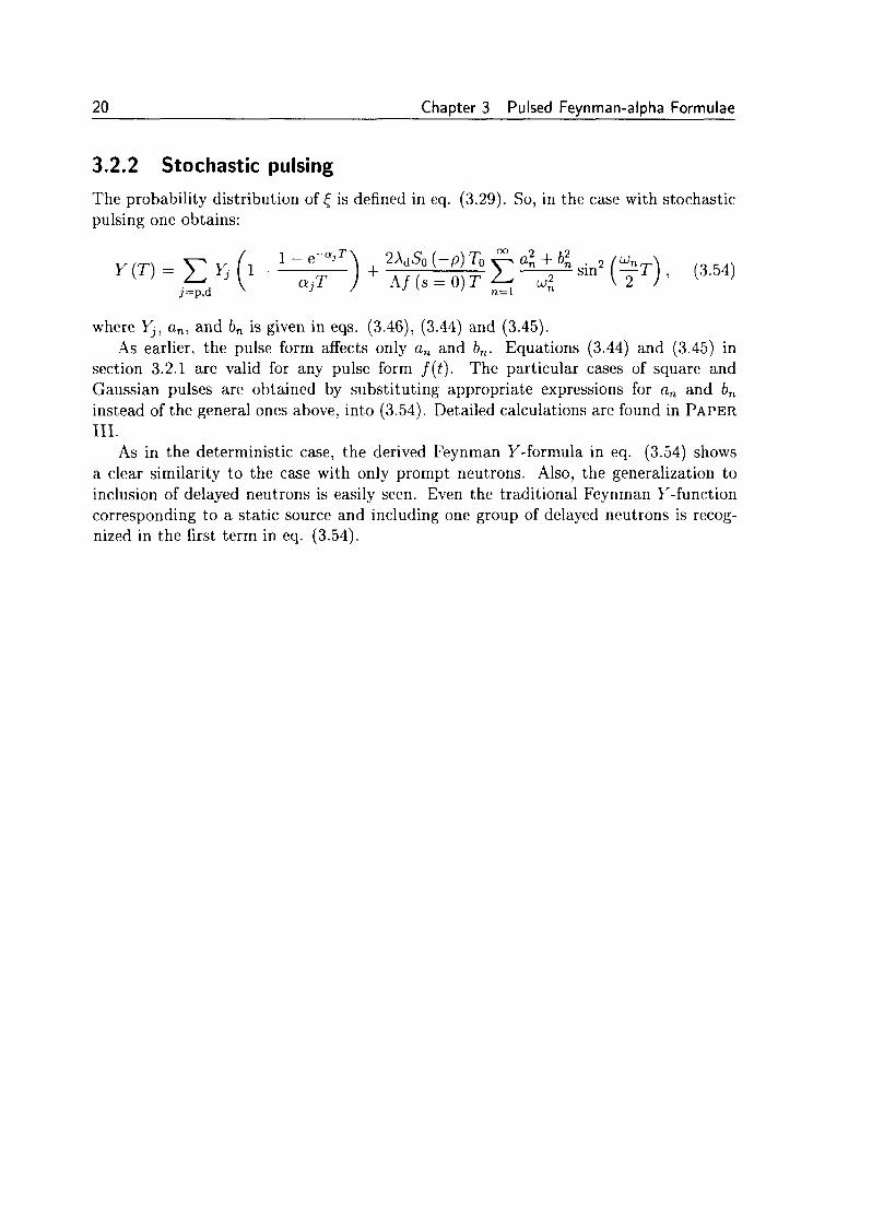
3.2.2 Stochastic pulsing
The probability distribution of £ is defined in eq. (3.29). So, in the case with stochasticpulsing one obtains:
where Yj, an, and bn is given in eqs. (3.46), (3.44) and (3.45).As earlier, the pulse form affects only an and bn. Equations (3.44) and (3.45) in
section 3.2.1 are valid for any pulse form f(t). The particular cases of square andGaussian pulses are obtained by substituting appropriate expressions for an and bn
instead of the general ones above, into (3.54). Detailed calculations are found in PAPER
III.As in the deterministic case, the derived Feynman F-formula in eq. (3.54) shows
a clear similarity to the case with only prompt neutrons. Also, the generalization toinclusion of delayed neutrons is easily seen. Even the traditional Feynman F-functioncorresponding to a static source and including one group of delayed neutrons is recog-nized in the first term in eq. (3.54).

4Source Modulation Method
In the previous chapter we described the Feynman-alpha method for subcritical mea-surements. In the present chapter we continue with the source modulation method.Since the method is based on the point reactor approximation, in section 4.1 the ki-netics of subcritical cores with a source is briefly revisited. Then, in section 4.2 wecontinue with a short derivation of the proposed formula, analyse its performance, andbriefly describe a possible improvement of the method. Detailed derivations are foundin PAPER IV.
4.1 Kinetics of subcritical cores
In this section, the same one-dimensional bare reactor model with one group of delayedneutrons as in [23] is used, but with slight change of the notation for better clarity forthe case of the subcritical kinetics. There is a need to distinguish between three differ-ent quantities; the static (and now subcritical) equilibrium state, the time-dependentquantities, and also the fundamental flux or adjoint, with corresponding buckling, whichbelongs to a hypothetical critical system. Therefore, we denote the static core quantities,belonging to the subcritical case, by a subscript p; the fundamental mode eigenfunc-tion with a subscript zero, and the time dependent quantities have no subscript. Thesource, which is unaffected by the reactivity of the system, is excepted from the aboveconvention and has a static value denoted by a zero subscript and a time-dependentdeviation.
In a one-dimensional homogeneous one-group diffusion model the static equationwith a steady source reads as
D V20p(x) + (i/E, - Ea) (j>p{x) + So(x) = 0. (4.1)
The usual diffusion theory boundary condition is given as
= 0, (4.2)
where xB is any of the two boundaries of the system. The other symbols have their usualmeaning. The system is assumed to be subcritical, i.e. keff < 1, and the subcriticalitycan be calculated from the eigenvalue equation for the critical flux.
Solving equation (4.1) with Green's function technique gives
<f>p{x) = fG(x,x')S0(x')dx', (4.3)
21

22 Chapter 4 Source Modulation Method
wheres'm[Bp(a - x')\ sin[Bp(a + x)]
G{x,x')= <DBP sin(2Spa)
s'm[Bp(a +x')]sm[Bp(a —x)} ,(4.4)
DBp sm(2Bpa)
with Bp being defined as
G(x, x') in eq. (4.4) is the solution to the corresponding static Green's function equation
V2xG(x, x1) + Bp G{x, x') + j;${x- %') = 0- (4.6)
Now, assume that the fluctuations of the flux are induced by the temporal and spatialvariations of the external source. We use the one-dimensional space-time dependentdiffusion equations:
+ [ ( 1 _ _ E a ] t)
( 4 7 )
with the boundary conditions
)=0. (4.8)
Inserting the time-dependent quantities split up into stationary values and fluctuationsin eq. (4.7), subtracting the static equations and eliminating the fluctuations of delayedneutrons by a temporal Fourier-transform, for the neutron noise in frequency domainfollowing equation is obtained:
V26(j)(x, u) + B2p{u)5(j){x, u) + -^ 6S{x, u) = 0, (4.9)
where
1 - — i — ) . (4.10)
GQ(UJ) is the usual zero transfer function, given by
(4.11)
L loj + A
which is similar to the critical zero reactor transfer function, but with material parame-ters of the actual subcritical system. As in the critical case, Go(u>) diverges for vanishingfrequencies.
Equation (4.9) can also be solved using the corresponding Green's function equation.The solution of eq. (4.9) is given as
6<j>(x,u)= fG(x,x',u)6S(x',Lj)dx', (4.12)

4.1 Kinetics of subcritical cores 23
where G(X,X',LJ) is the dynamic Green's function
,
G{x,x',u) =
' sm[B(u){a - x')} sin[B(uj)(a + x)]DB{UJ) sm(2B(u)a)
sin[B{u)(a + x')] sm[B(u){a - x)]DB{u) sm(2B{uj)a)
(4.13)
4.1.1 Point reactor approximation
In general, the reactor kinetic approximations are based on a factorisation of the space-time dependent flux into an amplitude factor and a shape function. In the one-dimensionalcase we have:
<P(x,t) = P(t)iP(x,t), (4.14)
where P(t) is as usual the amplitude function and ip(x, t) the shape function. For thesubcritical system we use the same definition of the point reactor approximation as isused by Pazsit and Arzhanov [23], and in PAPER IV, i.e.
</>{x,t) = P{t)<j>p{x), or rf>{x,t) = 4>p(x) V i (4.15)
where <j)p{x) is the static subcritical flux.Linearising by splitting up all the time-dependent quantities into mean values and
fluctuations and then inserting the linearised quantities in eq. (4.14) and neglecting thesecond order terms gives
6(j){x, t) = 4>(x)5P(t) + 5ip{x, t). (4.16)
Using the point kinetic equations for the fluctuations, the solution in frequency domainis
SP{u) = AGp(u)6q{uj), (4.17)
and the point kinetic approximation gives
6<t>pk{x,u) = \Gp{u})6g(u)(t>p(x), (4.18)
where Gp(u), is the zero-transfer function of the subcritical system:
Gp(u) = — 1—— . (4.19)iu A + , - p
The point kinetic solution (4.18) does not diverge for UJ —> 0, as it is expected, due tothe appearance of the reactivity in the denominator of (4.19).
4.1.2 Kinetics of subcritical cores with a source
For the source modulation method it is interesting to investigate the performance ofthe point reactor approximation for a variable strength source. In general, the validityof the point kinetic approximation depends on the frequency of the perturbation and
24 Chapter 4 Source Modulation Method
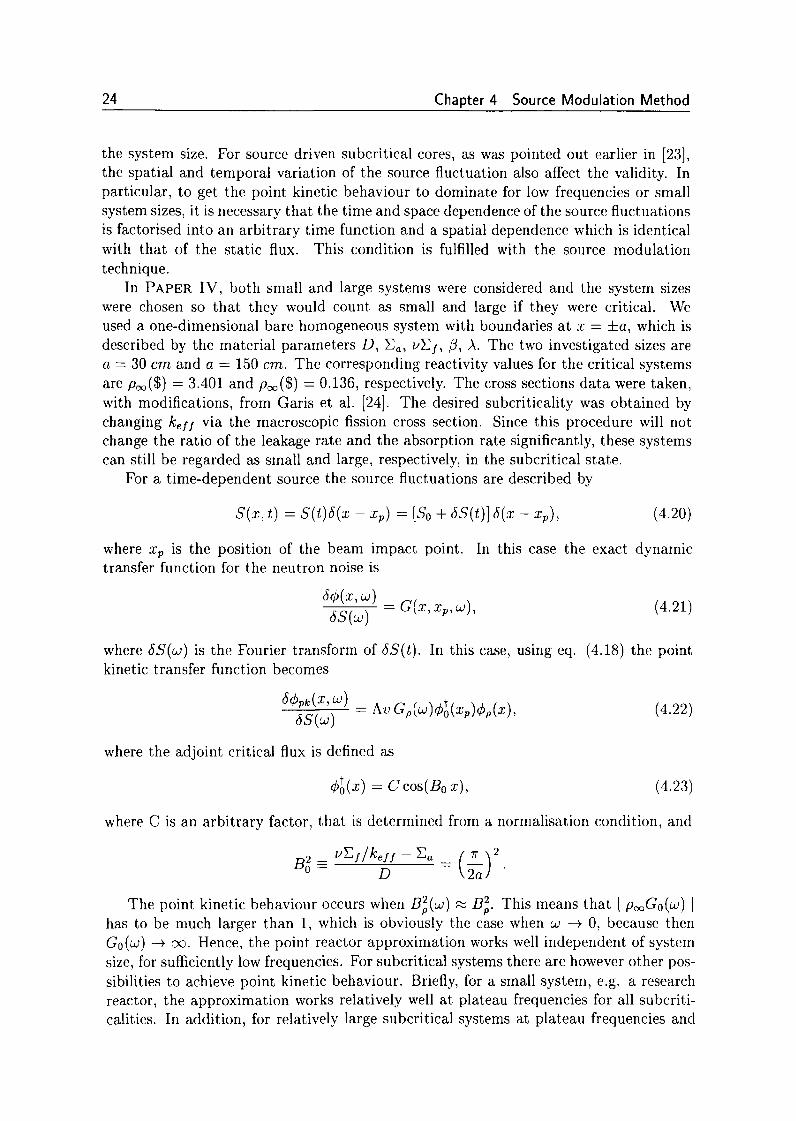
the system size. For source driven subcritical cores, as was pointed out earlier in [23],the spatial and temporal variation of the source fluctuation also affect the validity. Inparticular, to get the point kinetic behaviour to dominate for low frequencies or smallsystem sizes, it is necessary that the time and space dependence of the source fluctuationsis factorised into an arbitrary time function and a spatial dependence which is identicalwith that of the static flux. This condition is fulfilled with the source modulationtechnique.
In PAPER IV, both small and large systems were considered and the system sizeswere chosen so that they would count as small and large if they were critical. Weused a one-dimensional bare homogeneous system with boundaries at x = ±a, which isdescribed by the material parameters D, S a , t/£/, /?, A. The two investigated sizes area = 30 cm and a = 150 cm. The corresponding reactivity values for the critical systemsare Poo($) = 3.401 and Poo($) = 0.136, respectively. The cross sections data were taken,with modifications, from Garis et al. [24]. The desired subcriticality was obtained bychanging keff via the macroscopic fission cross section. Since this procedure will notchange the ratio of the leakage rate and the absorption rate significantly, these systemscan still be regarded as small and large, respectively, in the subcritical state.
For a time-dependent source the source fluctuations are described by
S(x, t) = S(t)5(x - xp) = [So + SS{t)] 6{x - xp), (4.20)
where xp is the position of the beam impact point. In this case the exact dynamictransfer function for the neutron noise is
where SS(OJ) is the Fourier transform of 8S(t). In this case, using eq. (4.18) the pointkinetic transfer function becomes
1 = Av GMtiWtpW, (4-22)
where the adjoint critical flux is defined as
<j^(x) = Ccos{B0x), (4.23)
where C is an arbitrary factor, that is determined from a normalisation condition, and
BB° = D
The point kinetic behaviour occurs when B2p(u) « B2
p. This means thathas to be much larger than 1, which is obviously the case when ui —> 0, because thenGo(u) —> oo. Hence, the point reactor approximation works well independent of systemsize, for sufficiently low frequencies. For subcritical systems there are however other pos-sibilities to achieve point kinetic behaviour. Briefly, for a small system, e.g. a researchreactor, the approximation works relatively well at plateau frequencies for all subcriti-calities. In addition, for relatively large subcritical systems at plateau frequencies and

4.2 Analysis of the performance of the source modulation method 25
k ,,=0.98, p ($)=-3.00Oil «
100 150 100 150
-300
-150 -100 -50 100 150 100 150
100 150
-150 -100 -50 0 50Position x [cm]
100 150
100 150
-150 -100 -50 50 100 150Position x [cm]
Figure 4.1: The noise induced by a fluctuating strength beam at various frequencies andPoo($) = —3.00 and for a large reactor. The solid line and the dashed line denotes theexact solution and the point kinetic approximation, respectively.
deep subcriticalities, where | /C»oo($) |3> 1, the system achieves point kinetic behaviour.This is shown in Fig. 4.1. In the figure, the exact and point kinetic transfer functionsfor a large reactor and for varying frequencies are shown. More detailed calculationsand figures for a small reactor are found in PAPER IV.
Summarizing, in contrast to critical systems where the only two factors determiningthe kinetic behaviour of the system is the frequency of the perturbation and the sizeof the system, in subcritical cores the static subcritical reactivity of the system alsoinfluences the kinetic behaviour. In the next section these conditions will be used in theanalysis of the source modulation method for reactivity measurements.
4.2 Analysis of the performance of the source modula-tion method
The source modulation method is based on the linearised point kinetic equations andtheir frequency domain solution for the amplitude factor fluctuation, 8P(to). Usingthe plateau frequency approximation, i.e. A < u C (j3 - P)/A, and introducing therelative fluctuations normalized by static values, 8P(u) and Sq(u), dividing the dynamicequation (4.17) with the static one, one obtains
SP(u) = (4.24)

26 Chapter 4 Source Modulation Method
which is the formula suggested by Carta and D'Angelo [14], for reactivity measurements.However, in reality only 6<J>(X,UJ) and (j)p(x) and not 5P(UJ) and Po can be measured.
To obtain an estimation of reactivity, SP(u) needs to be replaced with the normalisedspace-dependent flux 5<p(x,ui) = 5(j)(x,uj)/4>p{x) at some position x. The reactivity isobtained as
, „ , ( $ , x ) = - ^ " i • (4.25)5(p(x,uj) — oS{ui)
Using the exact solution for the neutron noise in the frequency domain and the staticflux for the model in Section 4.1, the accuracy of the estimation in eq. (4.25) can beinvestigated. This leads to
g ( ' X " ) ( 4 - 2 6 )G{x,xp,u) - G{x,Xp)
where G(X,XP,UJ) and G(x,xp) are denned in eqs. (4.13) and (4.4), respectively.The formula in eq. (4.26) can be generalised to all frequencies. Instead of using the
plateau frequency approximation the exact subcritical transfer function defined in eq.(4.19) can be used and then eq. (4.24) becomes
^ ) . (4.27)
For the estimated reactivity one obtains
(rr\ GQX{U)G(X,XP,U>)P^X) = G{X,XPM-G{X,XPY
(4'28)
where GQ{UJ) is defined in eq. (4.11).It is expected that the method will work well when the system behaviour is point
kinetic, which means that a measurement of the flux fluctuations in one point gives aproper approximation of the fluctuations of the point kinetic amplitude factor. Ourinvestigation, based on quantitative analysis of eq. (4.28), shows however that the ac-curacy of the method depends strongly on the detector position even when the systembehaviour is point kinetic. This is illustrated in Fig. 4.2, which shows the ratio of theestimated reactivity and the real reactivity for a large reactor with a = 150 cm, forijj = 20 rad/s, which is a typical plateau frequency. Subcritical reactivities correspond-ing to kejf equal to 0.9996, 0.99, 0.95, and 0.90, were chosen, or in dollars —0.061, —1.55,-8.10, -17.9. The corresponding p^ values are 0.0075, -1.42, -7.95, and -17.09, re-spectively. This system behaves point kinetically at plateau frequencies for k€jf < 0.99,as is shown in Fig. 4.1 for kefj = 0.98. Figure 4.2 illustrates that the estimated reac-tivity value shows large deviations from the reference value for all four subcriticalities.The conclusion is that for a large system the performance of the method is surprisinglypoor at plateau frequency.
For a small reactor the performance is reasonably good in slightly subcritical cases.However, it is interesting to note that with subcriticality levels that are more likely tobe used in planned power ADS, the method breaks down even in a small system atplateau frequencies. Since a large system is the more interesting case from the practical

4.2 Analysis of the performance of the source modulation method 27
-?50 -100 -50 0 50 100 150Position » (cm]
-f50 -100 -50 0 50 100 150Position x [cm]
f50 -100 -50 0 50 100 150Position x [cm]
-150 -100 -50 0 50 100 150Posilion x [cm]
Figure 4.2: The ratio of estimated and real reactivity for LO — 20 rad/s and differentsubcriticalities, for a large reactor with the source at the center of the core.
point of view, figures for the small reactor is omitted here and later. Nevertheless, theyare found in PAPER IV.
Since one could think that the reason for the large deviations is the large system sizeand the deviation from point kinetics even when this deviation is small, the performanceof the method was investigated in the point kinetic limit, i.e. when | p^ |—> oo or UJ —> 0.Here we describe briefly the latter case using the generalized formula, i.e. eq. (4.28).The other case, i.e. | p^ \—> oo leads to a similar result. Detailed calculations are foundin PAPER IV.
By defining e as
e =
a Taylor expansion gives for pasy, for xp = 0 for the leading term
x)cot(Bp{a + x))](4.29)
where f(x) is given as
1 - Bp [a ta,n(Bpa) - (a + x) cot(Bp(a + x))}2
1 — Bp [a t&n(Bpa) — (a - x) cot(Bp(a — x))}X p •
(4.30)
From the above for the ratio of the estimated reactivity to the true reactivity the fol-lowing relationship is obtained:
(4.31)

28 Chapter 4 Source Modulation Method
Consequently, the estimated reactivity has a finite error even when the system asymp-totically approaches point kinetic behaviour and regardless of how the limit is reached,i.e. by | p | —> oo or by u —> 0.
Figure 4.2 shows the asymptotic formula, eqs. (4.29)-(4.30), and the generalizedformula, eq. (4.28), for cu = 0.001 rad/s for a large system. The solid line and the linewith symbols denote the estimated ratio and the asymptotic ratio, respectively. The twoformulae agree well with each other. Except for the case of a very slight subcriticality,the error of the estimation is non-negligible. For the reactivity level planned for a futureADS, i.e. kefj « 0.95, the deviation between the estimated and true reactivity is quitelarge, even at this very low frequency.
*. 0.6
a] k e | | . 0.9996
-150 -100 -50 0 50 100 150Position x [cm] Position x [cm]
50 100 150
-100 -50 0 50 100 150Position x [cm]
-100 -50 0 50 100 150Position x [cm]
Figure 4.3: The ratio of estimated and real reactivity and the ratio of asymptotic andreal reactivity for ui = 0.001 rad/s and different subcriticalities, for a large reactor withthe source at the center of the core. The solid line the and the line with x denotes theestimated ratio and the asymptotic ratio, respectively.
4.3 Possible methods for improving the performance
The investigations in the previous Section showed that using a single neutron detector,unless it is by chance placed at a position where the theoretical error of the method iszero or very small, will give an error which will not disappear even in the limit of exactpoint kinetic behaviour of the system. However, the original formula was derived forthe amplitude factor of the factorised neutron noise, i.e. 8P(u) and not for the space-dependent noise 5(p(x,ui). The amplitude factor SP(UJ) can be recovered from S(f)(x,uj)as
5P(u)= 6<t>{x,u)<pl{x)dx. (4.32)
In other words, instead of using the local signals, a weighted integral, yielding theamplitude factor, could be used in the applications of the method. Using the correct

4.3 Possible methods for improving the performance 29
8P(co) instead of the local flux fluctuations, means that there is no need for the systemto behave in a point kinetic way. Hence, the method can also be applied at plateaufrequencies in a large system at arbitrary subcriticality level.
By using several detectors distributed relatively evenly at different positions in thecore, and trying to approximate the integral as a sum, 5P(u) from (4.32) can be ap-proximated. A similar approach was used in other noise problems earlier, see [25]. Theequation (4.28) can be approximated as
= D(Bj fig)EIG(xt,xp,a;)cos(JBoa:t)dxIPest[ ' D(Bl - Bj) £ \ G{xu xp, u) cos{B0Xi)dxi - cos{B0xp)
[ " '
Obviously, the quality of this approximation depends on the number of the terms used inthe sum (i.e. number of detectors in the measurement), and on the relative positioningof the detectors. It is obvious that detectors both close to and far away from the sourceare needed to be able to eliminate the space dependent term 6ip(x,uj) in eq. (4.16).
The applicability of this procedure was investigated quantitatively. Briefly, it isfound that the number of detectors needed is most likely larger than the number ofdetectors available for the purpose of reactivity monitoring in practice. Hence, themethod of summing up the detector signal fluctuations does not give the expectedmeasure of improvement of the method. In a real case the situation may be even moredisadvantageous, since in contrast to the investigations here that used a one-dimensionalmodel, the dynamics is three-dimensional and the space-dependent effects are even moresignificant. Hence, the source modulation method can most likely only be used in arelative way, after having been calibrated by other methods.

30 Chapter 4 Source Modulation Method

5Concluding remarks
In this thesis two subcriticality measurement methods were investigated, the pulsedFeynman-alpha method and the source modulation method. For the pulsed Feynman-alpha formula an efficient Fourier series solution method was developed, which can beused for any pulse shape. During the investigation of the source modulation method theconditions of point kinetic behaviour in subcritical cores were revised. The investigationled to the unexpected conclusion that in practical applications of the method difficultiesturn up when it is implemented by using single detector signals to approximate the pointkinetic amplitude factor. Hence, the source modulation method can most likely only beused in a relative way, after having been calibrated by other methods.
The results regarding the Feynman technique have been confirmed experimentallyin measurements made at the KUCA reactor of the Kyoto University Research ReactorInstitute. The results were also used in the interpretation of pulsed Feynman-alphameasurements within the EU project MUSE, and are likely to be used in future ADSprojects. There is no experimental application of the source modulation technique yet,but the conclusions have a clear relevance on the usefulness of the method, and havethus to be taken into account in the planning of future experiments.
In the continuation of this work, the experience gained in the work so far will beapplied to investigate the performance of the Cf-252 method. A formalism, similar tothat used in the study of the Feynman-alpha method will be used, but the aspectsof space-dependence, as well as the significance of point kinetic behaviour will also beinvestigated. Another method that might have practical relevance is the so-called breakfrequency method, whose applicability will also be investigated.
31

32 Chapter 5 Concluding remarks
Bibliography
[1] J. N. Wilford and M. L. Wald, A flash, and an uncontrolled chain reaction, TheNew York Times A.I (1999). New York, Oct 1, 1999.
[2] Science and technology: All over in a flash, The Economist 353, 102 (1999).London, Oct 9, 1999.
[3] IAEA report on the preliminary fact finding mission following the accident at thenuclear fuel processing facility in Tokaimura, Japan, (1999).
[4] IAEA nuclear safety review for the year 2003, (2004).
[5] 0 . Sandervag, (2002). Personal communication.
[6] R. Soule, W. Assal, P. Chaussonnet, C. Destouches, C. Domergue, C. Jammes,J.-F. Lebrat, F. Mellier, G. Perret, G. Rimpault, H. Serviere, G. Imel,G. Thomas, D. Villamarin, E. Gonzalez-Romero, M. Plaschy, R. Chawla,J. Kloosterman, Y. Rugama, A. Billebaud, R. Brissot, D. Heuer, M. Kerveno,C. L. Brun, J.-M. Loiseaux, O. Meplan, E. Merle, F. Perdu, J. Vollaire andP. Baeten, Neutronic studies in support of ADS: The MUSE experiments in theMASURCA facility, Nuclear Science and Engineering 148, 124-152 (2004).
[7] G. Imel, D. Naberejnev, G. Palmiotti, H. Philibert, G. Granget, L. Mandard,R. Soule, P. Fougeras, J. Steckmeyer, F. R. Lecolley, M. Carta, R. Rosa,A. Grossi, S.Monti, V. Peluso and M. Sarotto, The TRADE source multiplicationexperiments, in Proc. PHYSOR 2004 - The Physics of Fuel Cycles and AdvancedNuclear Systems: Global Developments. 2004. Chicago, Illinois, April 25-29, 2004.
[8] C. Rubbia, M. Carta, N. Burgio, C. Ciavola, A. D'Angelo, A. Dodaro,A. Festinesi, S. Monti, A. Santagata, F. Troiani, M. Salvatores, M. Delpech,Y. Kadi, S. Buono, A. Ferrari, A. Herrera, Martinez, L. Zanini and G. Imel,Neutronic analyses of the trade demonstration facility, Nuclear Science andEngineering 148, 103-123 (2004).
[9] N. Sjostrand, On the theory underlying diffusion measurements with pulsedneutron sources, Arkiv for Fysik 15, 147-158 (1959).
[10] F. de Hoffman, The Science and Engineering of Nuclear Power, vol. 2.Addison-Wesley, Cambridge, 1949. Chapter 9.
33

[11] R. Feynman, F. de Hoffman and R. Serber, Dispersion of the neutron emission inU-235 fission, Journal of Nuclear Energy 64-69 (1956).
[12] L. Pal, On the theory of stochastic processes in nuclear reactors, II NuovoCimento 7 (Suppl.), 25-42 (1958).
[13] J. Orndoff, Prompt neutron periods of metal critical assemblies, Nuclear Scienceand Engineering 2, 450-460 (1957).
[14] M. Carta and A. D'Angelo, Subcriticality-level evaluation in accelerator-drivensystems by harmonic modulation of the external source, Nuclear Science andEngineering 133, 282-292 (1999).
[15] J. Mihalczo, E. Blakeman, G. Ragan and E. Johnson, Dynamic subcriticalitymeasurements using the 252 Cf-source-driven noise analysis method, NuclearScience and Engineering 104, 314-338 (1990).
[16] J. Mihalczo and V. Pare, Theory of correlation measurement in time ansfrequency domains with 252Cf Annals of Nuclear Energy 2, 97-105 (1975).
[17] I. Pazsit, M. Ceder and Z. Kuang, Theory and analysis of the Feynman-alphamethod for deterministically and randomly pulsed neutron sources, NuclearScience and Engineering 148, 67-68 (2004).
[18] B. Sevast'yanov Uspekhi Matematicheskikh Nauk 6, 47 (1951).
[19] I. Pazsit and Z. Kuang, Reactivity monitoring in ADS with neutron fluctuationanalysis, in Proceedings of Topical Meeting on AccelaratorApplications/Accelerator Driven Transmutation Technology Applications '01.November 11-15, 2001. Reno, Nevada.
[20] Y. Kitamura, K. Taguchi, A. Yamamoto, Y. Yamane, T. Misawa, C. Ichihara,H. Nakamura and H. Oigawa, Application of variance-to-mean technique tosubcriticality monitoring for accelerator-driven subcritical reactor, in Proc.IMORN-29. 2004. Budapest, May 17-19, 2004.
[21] M. Ceder and I. Pazsit, Analytical solution for the Feynman-alpha formula for adswith pulsed neutron sources, Progress in Nuclear Energy 43, 429-436 (2003).
[22] I. Pazsit and Y. Yamane, The backward theory of Feynman- and Rossi-alphamethods with multiple emission sources, Nuclear Science and Engineering 133,269-281 (1999).
[23] I. Pazsit and V. Arzhanov, Theory of neutron noise induced by source fluctuationsin accelerator-driven subcritical reactors, Annals of Nuclear Energy 26, 1371-1393(1999).
[24] N. Garis, I. Pazsit and D. Sahni, Modelling of a vibrating reactor boundary andcalculation of the induced neutron noise, Annals of Nuclear Energy 23, 1197-1208(1996).
34

[25] J. Karlsson and I. Pazsit, Noise decomposition in BWRs with applications tostability monitoring, Nuclear Science and Engineering 128, 225-242 (1998).
35

36
Abbreviations
ADS Accelerator Driven Systems
APSD Auto-Power Spectral Density
B W R Boiling Water Reactor
CPSD Cross-Power Spectral Density
KUCA Kyoto University Critical Assembly
MUSE Multiplication avec une Source Externe
P W R Pressurised Water Reactor
SIRM Start-up and Intermediate Monitors
37


Paper I


CTH-RF-179 March 2004
Derivation and analysis of theFeynman-alpha formula for
deterministically pulsed sources
J. Wright and I. Pazsit
Department of Reactor PhysicsChalmers University of Technology
SE-412 96 Goteborg, SwedenISSN 0281-9775


CTH-RF-179
Derivation and analysis of the Feynman-alpha formulafor deterministically pulsed sources
J. Wright and I. Pazsit
Department of Reactor Physics, Chalmers University of TechnologySE-412 96 Goteborg, Sweden
Abstract
The purpose of this report is to give a detailed description of the calculation of theFeynman-alpha formula with deterministically pulsed sources. In contrast to previouscalculations [1], Laplace transform and complex function methods are used to arrive at acompact solution in form of a Fourier series-like expansion. The advantage of this method isthat it is capable to treat various pulse shapes. In particular, in addition to square- and Dirac-delta pulses, a more realistic Gauss-shaped pulse is also considered here. The final solution ofthe modified variance-to-mean, that is the Feynman Y(t) -function, can be quantitativelyevaluated fast and with little computational effort.
The analytical solutions obtained are then analysed quantitatively. The behaviour of thenumber of neutrons in the system is investigated in detail, together with the transient thatfollows the switching on of the source. An analysis of the behaviour of the Feynman Y(t)-function was made with respect to the pulse width and repetition frequency. Lastly, thepossibility of using the formulae for the extraction of the parameter alpha from a simulatedmeasurement is also investigated.
-1-

CTH-RF-179
1. Introduction
The theory of the Feynman-alpha method with pulsed sources became interesting recentlyin connection with the future accelerator-driven systems (ADS). An ADS is a subcritical reactordriven by a strong external neutron source. The source needs to be an accelerator-based one, inorder to achieve sufficient intensity. The most frequently proposed candidate for such a sourceis based on the spallation reaction. Due to technical reasons, such accelerators will most likelybe operated in a pulsed mode. This is also the case with the international MUSE project, whichis a 5th FrameWork program of the EU, for the experimental verification of some basic ADSprinciples. The MUSE experiments are being performed on a fast research reactor calledMASURCA, driven by a pulsed neutron generator called GENEPI [2]. The calculationsdescribed in this report were partly made for the theoretical support of evaluation of the MUSEexperiments.
There are different ways of describing a pulse of neutrons from a neutron generator. Onepossibility is to assume a finite pulse width, usually with a square shape, and assume that duringthe pulse all neutrons arrive at random with Poisson statistics. In between the pulses there are noneutrons emitted. This method was used in Refs [1], [3]-[5], and this is also the approach thatwe shall pursue in this report, although here both square and Gaussian-shaped pulses will beconsidered. The other possibility is to assume that the pulses have the width of a Dirac deltafunction in time, but at each pulse a random number of neutrons is injected into the system. Thisapproach was used in Refs [6]-[8]. In certain special cases the results from the two methods arequantitatively equivalent, as it will be touched upon in the report.
In either cases, i.e. either finite width or infinitely short pulses, there are still twopossibilities to perform or evaluate measurements. These are generally termed as deterministicand stochastic pulsing, respectively. The deterministic pulsing means that the start of themeasurement, i.e. neutron detection or pulse counting in the neutron detector, is synchronisedwith the source pulse train. The usual assumption is that the neutron detection always starts atthe start of a pulse from the neutron generator. The stochastic pulsing means, as the nameindicates, that the neutron detection and the source pulsing are not synchronised, so that the startof the neutron measurement is randomly distributed with a uniform probability over a timeperiod of the source pulse.
For the case of finite sources, which is also our subject here, both the deterministic ([1],[5]) and the stochastic ([4], [5]) pulsing was treated earlier. However, in these earlier works thecase of the deterministic pulsing was treated with a method such that the correspondingtemporal differential equations were solved piece-wise for each consecutive pulse and theperiods in between the pulses [1]. Although the method did yield quantitatively correct resultswith very short computation times, it was at the same time clumsy to use for different values ofthe input parameters, and did not appear to be suitable for parameter unfolding by curve fitting.
Another, more significant drawback was that the solution method was based on thepiecewise constant behaviour of the source. Extension of the method to more complicated (andhence realistic) pulse shapes would incur a substantial complication.
In the case of stochastic pulsing, another approach was used. It was noticed that severalexpressions for the first and second moments of the neutron number and the number ofdetections were, or could be cast into, the form of convolutions. One could make use of the factthat the Laplace transform of such convolutions could be written as the product of the individual
-2-

CTH-RF-179
Laplace transform, and the original convolution could be obtained in the time domain through aLaplace inversion by complex function methods. It was therefore suggested that also the case ofdeterministic pulsing also be treated this way, and even the feasibility was demonstrated [5].However, in order to arrive to tractable compact results, a significantly larger effort was neededthan in the case of stochastic pulsing. This was only achieved relatively recently.
It was immediately realised, that this method could be extended to other pulse shapes, andin particular to a Gauss-shaped pulse, which is actually the case of the pulses of the neutrongenerator GENEPI in the MUSE experiments. In fact, the singularity structure (number andposition of the poles) of the function to be inverse transformed is determined only by theperiodicity of the source pulse train, and it is only the values of the residues at these poles thatare dependent on the actual pulse form. This means that it is only a relatively small part of thecalculations that needs to be re-done when calculating the Feynman-alpha function for variouspulse shapes. This is demonstrated in the report by calculating the y-function for both squarepulses and Gaussian pulses.
The purpose of this report is to describe the flow of these calculations in a detail that islarger than what is customary in a journal publication. Also, based on the compact form results,a qualitative and quantitative analysis of the Feynman-alpha formula is made and reported, whatregards the dependence of the characteristics of the Y(t) -curve for various combinations of thepulse width and repetition frequency. Finally, the possibility of extracting (unfolding) theparameter alpha from some simulated measurements, generated by the formulae derived andadding some extra noise, is investigated. These show that the formula is suitable for thedetermination of subcritical reactivity from Feynman-alpha measurements with deterministicpulsing, given that the pulse period is short enough in comparison to 1 / a .
2. General theory
The principles and the basic theory of the Feynman-alpha method are described in severalpublications, including the pre-decessors of the present work (e.g. in [1], [3] and [5]). Themethod is based on the measurement of the detector counts Z(T) during a measurement timeperiod T in a stationary system driven with a source S. Both the source emission, the diffusionand multiplication of the neutrons in the medium, as well as the detection process, are subject torandom fluctuations. The probability of emission of a source neutron during time t is given asSdt. The condition of stationarity requires that the measurement is made a long time after thatthe source was switched on, such that all transients after the switch-on have decayed. With arepeated measurement of the random variable Z , its mean (Z) s Z and variance oz( T) can bedetermined. With a repetition of the measurement for various measurement time lengths, thedependence of the relative variance, or the variance-to-mean <5Z{T)/Z (Feynman-alphafunction) can be determined. In practice, it is more customary to use the deviation of the relativevariance from unity, which is called the Feynman y-function:
(1)Z{T) Z(T)
where
(2)
-3-

CTH-RF-179
is called the modified variance. The advantage of introducing the modified variance is theconvenience that one can derive equations for it directly.
The mean and the variance of the detector counts can be calculated from a master equation,i.e. from a probability balance equation. Usually, it is more advantageous to use the so-calledbackward master equation, which means that one has to operate on initial variables [9]. Thisexcludes the possibility to switch on the source in -<», rather it is assumed that the source isswitched on at t = 0 and the measurement is made when t —» °° . For this reason one needs togo in two steps; first the probability of the number of neutrons in the system and detector countsduring the time period (t - T, t) is determined, and then from this the probability of the samequantities is calculated for the case of an external source.
Because we shall be dealing with a time-dependent source, which constitutes acomplication compared to the previous cases, for the time being we shall neglect the existenceof the delayed neutrons in this work. They will be treated in a coming publication.
The quantities that will appear in the derivation are thus as follows.
P(N, Z, t) (3)
is the probability of finding N neutrons at t and Z counts in the time interval {t -T, t), due toone neutron starting the process at t = 0. One also introduces the probability generatingfunction of P as
Z,t) (4)N Z
If a master equation for the generating function G is obtained, equations for the variousmoments can be obtained by differentiating G w.r.t. x or z. Such a master equation was deriveda long time back in the theory of neutron fluctuations in nuclear reactors. For later reference, weonly quote the two first-moment quantities that will be used in later parts of the paper in thecalculations. The expected number of neutrons at time t is given by
N(t) = e~al (5)
where a is the prompt neutron time constant, given by a = - p / A . Here p is the subcriticalreactivity (to be determined in the measurement) and A the prompt neutron generation time.Both p and A can be expressed by nuclear physics parameters such as cross sections andneutron speed, and are known in a calculation.
The second quantity we shall need is the expected number of counts, which is given as
t
Z{t,T) = \d\N{t-n&(f,T)df (6)
o
where
[ 0 < t < T( 7 )
From (5)- (7) it readily follows that
-4-

CTH-RF-179
t
Z(t, T) = \dJHf, T)N(t-t')dt' =0
_2(i_ e-o«). 0<t<T
" (8)
a
In a similar manner,
P(N,Z,t\t0) (9)
denotes the probability of finding N neutrons at t and Z counts in the time interval (0, t), dueto a source being switched on at t = tQ. As it is usual in the literature, all distributions andmoments, corresponding to the source-induced case, will be denoted by a tilde. The generatingfunction of P is defined as
G(x, z, t\t0) = JtJ^x'z"P(N, Z, t\t0) (10)N Z
As it will be seen in the next section, one can derive a direct relationship between G and Gsuch that the latter is given as an exponential integral over the former. Calculation of themoments of the source-induced distribution requires in general the calculation of multiplenested integrals over certain functions of the various moments of the single-particle induceddistribution.
3. Calculation of the Variance-to-mean for Deterministically PulsedSources
As mentioned earlier, the novelty of the Feynman-alpha method with a pulsed sourceconsists of the time dependence of the source. Some characteristic properties follow directlyfrom the fact that the source consists of a train of pulses, independently of the form of thepulses. These will be first investigated here. For the sake of concreteness, whenever explicitformulae are necessary, square pulses will be assumed. The case of Gaussian pulses will betreated in Subsection 3.5.
3.1. The source and its Laplace transform for square pulses
The time-dependent neutron source is represented by a sequence of square functions:
(11)
where H is Heaviside's step function, To the pulse period, and W the pulse width. In Fig. 1 thefunction is plotted.
The Laplace transform of the source is given by:
W e n -sW\S(s) = je~slS(t)dt = Y,(e~sTo)"So\e-sldt = — ^ ^ — ; Re{s}>0. (12)
o 0 o s(l-e °)
Eqn (12) shows that the singularities of S(s) are determined by the zeros of the denominator,
-5-
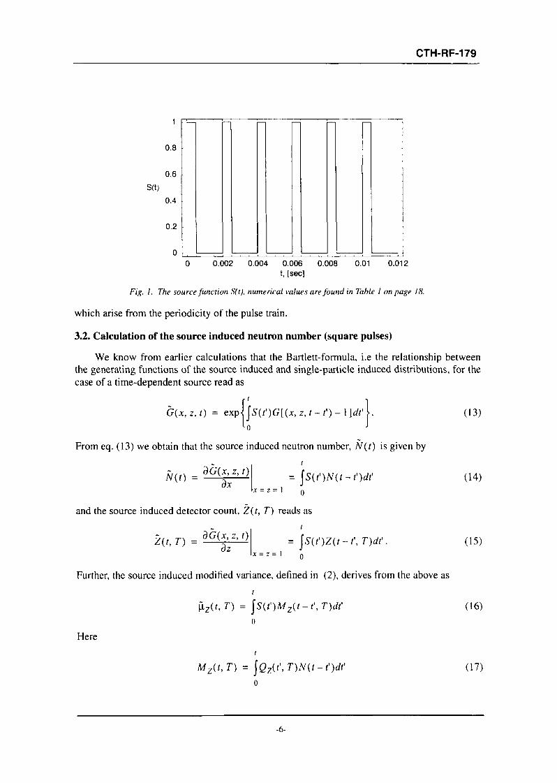
CTH-RF-179
S(t)
0.8
0.6
0.4
0.2
00 0.002 0.004 0.006 0.008 0.01 0.012
t, [sec]
Fig. I. The source function S(t), numerical values are found in Table 1 on page 18.
which arise from the periodicity of the pulse train.
3.2. Calculation of the source induced neutron number (square pulses)
We know from earlier calculations that the Bartlett-formula, i.e the relationship betweenthe generating functions of the source induced and single-particle induced distributions, for thecase of a time-dependent source read as
d(jc,z,0 = expUS(t')G[(x,z,t-O-\}dA. (13)
From eq. (13) we obtain that the source induced neutron number, JV(/) is given by
N{t) =dG(x,z,t)
dx X = 2 = 1
= ^S{t')N{t-t')dt' (14)
and the source induced detector count, Z(t, T) reads as
~Z(t, T) =dz
= \S{OZ{t-t\T)dt\ (15)
Further, the source induced modified variance, defined in (2), derives from the above as
Here
ViZ{t,T) = \S(t<)Mz{t-t\T)dt'
Mz(t,T) = \Qz(t',T)N((-f)dt'
(16)
(17)
-6-

CTH-RF-179
with
Qz(t,T) = \f(v(v-\))Z2(t, T). (18)
and where Z(t, T) is the single-particle induced detector count, given in eq. (8). Hence, usingeq. (14) and eq. (15) we can write eq. (16) as
i
\iz{t, T) = \Qz(t\ T)N(t - t')dt'. (19)
o
The Laplace transform of eq. (14) is
N(s) = S(s)N(s) (20)
where
N(s) = — (21)s + a
since
N(t) = <ra' (22)
where a - -- and p = —;— as usual.A k
Hence
N(s) = u e / , (23)
s{l-e-sT°)(s + a)
From eq. (23) we can obtain N(t) with inverse Laplace transform. Let
N(s) = (\-er*w)f{s) (24)
where
5(1 -e s'°)(s + a)
then
f/(0 t<WN(t) = f(t) - H{t - W)fit -W) = \J"[ ^ . _ _ m ( 26 )
For the inversion of eq. (23), we note that its singularities are defined by three different types ofpoles, each corresponding to a different type of behaviour in the time domain after inversion.
1. A pole at s = 0; the corresponding residue gives the asymptotic mean value of theoscillating function N(t);
2. a pole at 5 = - a , which describes the transient after switching on the source at t = 0;
3. an infinite number of complex conjugate roots on the imaginary axis, yielding harmonicfunctions in the time domain, representing a Fourier series expansion of the oscillating partof N(t).
-7-

CTH-RF-179
As mentioned earlier, the positions of these poles are independent of the form of the pulseshape, because they are given by the zeros of the function (1 - e~sT°), which latter was givenrise by the summation of the geometric series in (12) expressing the periodicity of the pulse. It isonly the value of the residues which is affected by the pulse shape. In other words, the result forthe asymptotic value of Na(t) can always be written in the form of eq. (35) below, only thevalues of the an and bn will be different.
Let us write now the inverse Laplace transform of eq. (23) in terms of the inverse of thefunction f{s), introduced in (25), in a sum corresponding to the three types of poles above.That is, let us write f(t) = c{t) + e(t) + g(t) and calculate each term separately. Then thetheorem of residues gives:
c{t)=Res2(ta-
= o s{\-e-sTn
(27)
c-al
e(t) == -a s( 1 - e~sT° )(s + a) «(1 -
(28)
and
sin — - a r o - c o s —— Ylnno c o s
n - 1
(29)
Hence, also in view of eq. (26), one has
N(t) = c(t) + e(t) W). (30)
A plot of N(t) is shown in Fig. 2. It is obvious that after a number of pulses the initial transientdecays and the system converges to an asymptotic state.
0.0004
0 0.002 0.004 0.006 0.008 0.01 0.012t, [sec]
Fig. 2. N(t) with its asymptotic behaviour indicated as a dotted line. Numerical values are found inTable 1 on page 18.

CTH-RF-179
When / -> oo, N(t) is simplified to:
wTQa
Using trigonometric identities and introducing a>n = -=— , we get1
(31)
where
and
= i
an =- cos(conW)]a + (£)nsm{bsn
(32)
(33)
(34)
Thus, the asymptotic source induced neutron number, Na(t), is
oo
W 1Na(t) =1 o a "n = 1
This function is shown in Fig. 3.
(35)
Na(t)
Na(t)-ggw(t)
0.002 0.004 0.006 0.008 0.01t, [sec]
0.012
Fig. 3. Na(t) and the constant term in Na(t) i.e. Na(t) — ggw(t). Numerical values are found inTable 1 on page 18.
As will be seen in the next two subsections, in all subsequent calculations of the source-induced asymptotic detector count Za{t) and the Feynman Y{t) -function, the solution givenfor Na{t) above is used in various nested integrals in combination with functions that do not
-9-

CTH-RF-179
depend on source properties. The functional dependence of Na(t) is given by the trigonometricfunctions that do not depend on the pulse shape. Hence in the resulting expressions using adifferent pulse shape means just changing the parameters an and bn and the first term on ther.h.s. of (35).
3.3. Calculation of the source induced detector count for arbitrary pulses
The single-particle induced detector count, Z(f, T) is given, as usual (c.f. eqn (8)):
I
Z(t, T) = \
o
— ( 1 -e-al); 0<t<T
x (36)
— e ~ a ' ( e a T - 1 ) ; t>T.
where A(f, T) was defined in (7)
From eq. (15) the source induced detector count, Z(t, T), is given by:
Z(t, T) = XdJA(t\ T)N(t - t')df . (37)
o
The easiest way to calculate the integral is not with the same method as was used for N{t) , i.e.writing the Laplace transform of Z(t, T) as:
(1 - e~sT) (1 - e~sW) 1
The reason is, that for eq. (38) it is rather complicated to use the same trick as for eq. (24) due tothe factor (1 - e~sT){ 1 - e~sW). Further, it is easier to let ?^«> in eq. (37) than in eq. (38).But, since we have a simple expression for Na(t), i.e. eq. (35), we are able to obtain theasymptotic source induced detector count by calculating the integral in eq. (37) when / —> °°.Thus,
t
Za(T) = lim kJw,T)Na(t-t')df. (39)
0
As a result of deterministic pulsing we have / = KT0 + T and it is obvious that letting t —> °oequals to letting K —> °° . With that, we have:
KT0+T KT0+T T
= Xd J &{t',T)Na{t-t')dt'= Xd I Na(t)dt = XdJNa{t)dt. (40)0 KT0 0
The last step above results from the periodic character of A ^ f ) . The above gives, with eq. (35):
-10-

CTH-RF-179
Za{T) = WT + i^-t (41)
Fig. 4 shows both the asymptotic source induced detector count, Za{t) and only the linear term,Z/, of Za{t). The oscillating part, Zosc, is plotted in Fig. 5. All curves are normalized with afactor
2(t)
— 2m• - - 2,(0
0.002 0.004 0.006 0.008 0.01 0.012t, [sec]
Fig. 4. Za(t) and the linear term Z/. The solid line denotes Za(t) and the dashed line Zj. Numericalvalues are found in Table 1 on page 18.
0 0.002 0.004 0.006 0.008 0.01 0.012t, [sec]
Fig. 5. The oscillating part Zosc, other numerical values are found in Table I on page 18.
-11-

CTH-RF-179
3.4. Calculation of the modified variance for arbitrary sources
The asymptotic modified variance is obtained from eq. (19) using the asymptotic sourceinduced neutron number, Na(t):
t
M'-H = JQz(t\T)Na(t-t')dt' (42)o
where Qz(t, T) is defined in eq. (18) with Z(t, T) given by eq. (36).
Let C = X,rf<v(v-1)> , and for / < T we define with eq. (36):
C ( £ ) l - e - « ' ) 2 (43)
and for t> T:
02(0 = C^e-2*T(eaT-\)2. (44)
Correspondingly, the expression for the modified variance, eq. (42) will be broken up into twoparts, i.e. £z(f, T) = \ix(T) + \i2(T), with ]xx(T) and \i2(T) corresponding to the integralsover £?,(/) and Q2(t), respectively. If we also let t = KTQ + T, we obtain:
T KT0 + T
ixz{KT0+T,T) = \Qx(t)Na{T-t)dt+ j Q2(t, T)Na(T - t)dt. (45)
0 T
When t —> °° :
T
UZ(KTO+T,T)= \Qx{t)Na{T-t)dt + \Q2(T +1, T)Na(-t)dt . (46)
o o
Using eq. (31) andeq. (32) the \ix(t)-integral becomes:
T r i ,„ T T
\Q\(T - t)ggw(t)dt. (47)
0 l J 0
Using eq. (43), the result of the first integral is:
(48)
T
W r~ , , , ^fXd\2 W 2Ta + 4e~aT - e~2aT - 3o roa 2a
The second integral in eq. (47) is trickier to evaluate. We notice that, according to eq. (43), wehave:
QAT-t) = C — (1 -e-vv-'iy = \~2e-alea< + e-Za'eZal. (49)
-12-

CTH-RF-179
ggw(t) is given by eq. (32). It is suitable to evaluate the integral in two parts. First, the one withthe sine and second, the one with the cosine functions. Now, let
Te a s i n ( a ) 7 ) + (a(e~aT - cos(co 7 ) )
Pn(a, r ) ^ - a r ea'sin(ay)A = - ^ - £—= y_JLJl. (50)
Then,
T
' 77 ) W ° ' r ) - 2Pn(<*> T) + P»&*> H ) . (51)o
Analogously, letT
asin(conr) + a>n
Then,
. (52)
2
^ j {qn(0, T) -2qn(a, T) + qn(2a, T)) (53)
andT
t)ggw(t)dt = C\ — I - V {an/4n(7') + bnBn(T)} . (54)
o «=i
Finally, we have from eq. (48) and eq. (54):
" W 2Ta + 4e-aT-e-2aT-3 \ y A
Using eq. (31) and eq. (32) the u 2 (0 -integral in eq. (46) becomes:
T r T
j f. (56)
o °The first term in the integral above results in:
" ' f ^ * . ^ . (57 ,
The first part of the ggw(t) -integral gives:
-13-
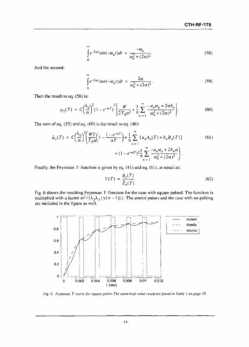
CTH-RF-179
e-2a'sin(-w t)dt =J " w2 +12
(58)
And the second:
(<?-2«'cos(-co t)dt = ^~J " w2 + (2a(2a)2 (59)
Then the result to eq. (56) is:
(60)
The sum of eq. (55) and eq. (60) is the result to eq. (46):
(61)
+ (1 -= 1 (2a)2
Finally, the Feynman K-function is given by eq. (41) and eq. (61), as usual as:
(62)
Fig. 6 shows the resulting Feynman F-function for the case with square pulsed. The function ismultiplied with a factor a2/{XdXj-(\(v - 1))). The source pulses and the case with no pulsingare included in the figure as well.
0.8
0.6
0.4
0.2 /
y 7
- — ^—
0 0.002 0.004 0.006 0.008 0.01 0.012t. [sec]
Fig. 6. Feynman Y -curve for square pulses. The numerical values used are found in Table 1 on page 18.
-14-

CTH-RF-179
3.5. The case with Gaussian pulses
It is possible to use Gaussian pulses instead of the square pulses in eq. (11). Then the time-dependent neutron source is represented by:
S(t) = -exp (63)
where a = W/4 and 5 = Jliza. The parameter s here plays the role of the source intensity,i.e. the same as SQ for the square pulses in (11). The parameter s here plays the role of thesource intensity, i.e. the same as SQ for the square pulses in eq. (11). Its numerical value doesnot play a role in the derivation of the formulae, since it drops out from the Feynman-alphafunction, which is one of the advantages of the variance-to-mean method. Hence its value waschosen such that the maximum value of the pulse function is unity. This choice has no othermotivation than easy comparison of the source forms in the plots. Likewise, the choice ofo = W/A is also arbitrary, and again was made in order that the square and Gaussian pulses becomparable. One representation of such a Gaussian train, with its square pulse companion withthe same repetition frequency and corresponding width W, is shown in Fig. 7.
W=0.OOO5,T0=0.OO5, o=W/4
n
i i
i ii <
I i
i i
j ii iI i
, i
[ i
y
] i
i '
i '
i
• i
i i
11
11
11
1 1
1 1
1 1
1 1
1 1
i t
square- gaussian
0 006t. (sec]
0.012
Fig. 7. The Gaussian pulse and the square pulse, W - 0.0005, TQ = 0.005, o = W/A, s = a Jin
The Laplace transform of Sn(t) is thenoo oo
Sn(s) = je-s'Sn(t)dt = e~nsT"jS0(t)e-s'dt; Re{s}>0. (64)
o o
The task is hence to calculate the integral for the term n - 0 . This can be simplified as follows:
-15-

CTH-RF-179
(65)
J2ni
As is seen, the lower limit of the integral was extended to minus infinity. The error committedby this step is rather small, given the fast decay of the Gauss function. This may not be soobvious when it is expressed in terms of the very first pulse, which starts close to the origin.However, for the later pulses it becomes a better and better approximation. Since the Feynman-alpha measurement relates to the stationary case, i.e. times long after the switching on thesource, the error committed by this approximation is indeed negligible. In return, it leads to acompact analytic form.
Thus, the Laplace transform of the sum in (65) is equal to
S(s) = ^ 2—— . (66)1 - s T
According to eq. (20) and eq. (21) we have:
-esT°
se 2 1N(s) = - — . (67)
1 _ esTo s + a
For the inversion of eq. (67) we note that the singularities are of the same three types as ineq. (23). We write the inverse Laplace transform, in a similar manner as for the square pulse, asf{t) - c{t) + e(t) + g(t) and calculate each term separately. Then the theorem of residuesgives:
-sW + (as)2
^ e 2 = - ^ - (68)T J a
-sW
{) ?f e 2 = Se aT e 2 (69)
and
e 2 = - X K s i n ( G y ) + 6ncos(Gy))- (70)
where
an =
2 \ ( W\ ( W\\--j ot7^0sinl cow— 1 + 27t«cosl ooM— IJ- (71)
-16-

CTH-RF-179
(72)
It is obvious that when (-><», e(0 —> 0 and the asymptotic source induced neutron number is:
(73)u .. _ i
where an and bn are as in eq. (71) and eq. (72), respectively.
Above, Na(t) is written in a similar way as in the case with the square pulse, i.e.oo
~ 1 (74)n = 1
where Cs is a constant that depends on the pulse form. Thus, we are able to use the sameformulas for the source induced detector count, eq. (41), and modified variance, eq. (61) as forthe square pulse with minor modifications. So, we have:
Za(T) = V fn = I
(75)
and
(76)« = 1
0)2 + (2a) 2 )
where /4n and /?„ are as in eq. (51) and eq. (53), respectively. The resulting Feynman Y-function is given by eq. (62), as usual.
Fig. 8 shows the resulting curve for both the Gaussian and the square pulse. In the Figure,the function is multiplied with a factor a2/{XdX^(v(v - 1))). The source pulses and the casewith no pulsing are included in the Figure as well. The Figure shows that the Y-curve due to theGaussian source shape is smoother than the one due to the square counterpart. This is because aGaussian pulse it does not contain sharp edges (discontinuous derivatives) as the squarefunction.
-17-

CTH-RF-179
W=0 0005 ,T.=0.004 .0=0 000125
gaussian-- - square- steady
0.01 0012
Fig. 8. Feynman Y-curve for Gaussian and square pulse. The numerical values included areW = 0.0005, TQ = 0.004, a = W/A, J = a Jin
4. Convergence of the Feynman r-function
In the numerical work that follows, in this and the following Section, the followingnumerical values will be used:
Table 1: Numerical parameters
Parameter
To
W
Sok
A
2
5
1
0
5
Value
io-3
• i o - 4
n/s
95
• io-5
s
s
s
With the above data, one obtains a = - p / A = 1052, 6 s
It is important to know how many terms in the sums in eq. (61) are necessary for adequateresults. One part of the asymptotic source induced detector count, Za(t), given in eq. (41) isoscillating. However, the sum Zosc converges relatively fast, see Fig. 9. In this figure, Zosc isplotted for increasing number, n, of terms in the sum, for some arbitrary values of time t. Forn=5 we get a relatively good approximation of Zosc.
-18-

CTH-RF-179
x 10"'
8 -
7
6
5
'C4
3
2
1
0 -
N
J
\ /
ll / °!
1 /A / °
1 / -OS
.'.yi/ \ ~2/ \
i 10'*• 1 1
/ Vi
^ r~\ J
\ : / •
• / : •
-
-
-
-
-
_
_ i ^
t=O.OO1t=0.0012
- 1=0.0015t=0.0O18
^— t=0.002
10 15
Fig. 9. Convergence of the oscillating part, Zosc, the inset magnifies the behaviour near zero.
For the two sums in \iz(T), in eq. (61) it is suitable to normalize the resulting sums withthe asymptotic value i.e. the value which includes n = 30 terms in the sum. This makes iteasier to evaluate for which n the approximation is good enough. Examples of the non-normalized sums are shown in Fig. 10. In this figure the first sum in p.z(T) is plotted.
x 10
3.5 -
3 -
2.5 -
2 -
1.5 -
0.£
• - • - • . _ _ . _ . _ . _ _ .
t=0.001t=0.0O12
- t=0.0015t=0.0018t=0.002
10 15n
2 0 2 5 3 0
Fig. 10. Convergence of the first sum in |I r( T), non-normalized values
-19-

CTH-RF-179
The first sum in | I z ( r ) , see eq. (61) is plotted in Fig. 11 for increasing number of terms, n.in the sum, for a few values of time t. The sum is normalized with the asymptotic value.
1.07
1.06
1.05
1.04
1.03
1.02
1.01
0.99
n Qft
A
\l\• v4r 'A
• n / ^./ kf
L(a n A n(t
—-— l
) + b n B n(1)); n=30
-
-
-
-
-
t=0.001- - t=0.0012- t=0.0015
t=0.0018t=0.002
Fig. 11. Convergence of the first sum in (iz( T) , normalized with the asymptotic value.
The second sum in eq. (61) is plotted in Fig. 12 for increasing number of terms, n, in thesum, for some arbitrary values of time / . The sum is normalized with the asymptotic value.
I 8
1.7
1.6
1.5
1.4
1.3
1.2
1.1
1
n Q
I
\
\
£ (-a ncon + 2a b n )/ (<o « +(2a)"); n=30
-
-
-
• -
-
t=0.001- - t=0.0012- t=0.0015
t=0.0018^— t=0.002
15n
3 0
Fig. 12. Convergence of the second sum in \iz{ T) normalized with the asymptotic value.
The figures above indicate that it is the second sum in j i , ( r ) that determines the value of nso the error is small enough. Therefore it is convenient to use « = 15.
-20-

CTH-RF-179
5. Analysis of the Behaviour
In this section a number of plots of Feynman F-function for a number of W- and TQ
values are presented. All curves are normalized with a factor a 2 / ( ^ L ( v ( v - 1))).
0,8 -
0 6
08
06
— pulsed- steady
0 006t. [sec]
0.008 001 0.012
Fig. 13. Feynman Y-curvefor W=0.001 and T0=0.002
W=1e-06.T0=0.002
11
I 1t
I 1I I
1 11 I
s /
— pulsed- steady
-
0.002 0 004 0.006t. [sec]
0 01 0,012
-6Fig. 14. Feynman Y-curvefor W=le'° and T0=0.002
The effect of the pulse width is illustrated in Figs 13 and 14 for square pulses. It is seen thatthe wider the pulse is, the smoother the curves become. This is not surprising, since thecontinuous source corresponds to the case when the pulse is as wide as the pulsing period,which gives a completely smooth curve. Fig. 14. corresponds to the pulsing with a very narrow
-21-

CTH-RF-179
pulse. Such results were obtained by other groups in Japan, and are in agreement with ourresults (Refs [6]-[8]).
For sake of comparison, a Feynman /-curve with Gaussian pulses, with the samerepetition frequency as with the square pulses above, is shown in Fig. 15. Despite that it
=O 0005 ,T=0.002 ,a=0 000125
~~I 1 1 1 ~1
1//
n l\ I
I —i
> • •
\ 1 ! \ 1 j
gaussiansquare
— steady
0.006t. [sec]
0 008 0.01 0012
Fig. 15. The resulting Feynman Y -curve for gaussian and square pulse, included numerical values areW = 0.0005, TQ = 0.002, o = W/4, J = aj2n
corresponds to much narrower pulses than the case in Fig. 13. for the square pulses, the Y-curve is just as smooth as for a wider square pulse. This is because of the smoother character ofthe Gaussian pulse shape.
The effect of the repetition frequency, with a given prompt neutron time constant, is shownin Figs 16-19. The figures show that for a sufficiently high repetition frequency (Figs 16 and17), the pulsed curve remains smooth and close to the continuous curve even for narrow pulses.The same conclusion has been drawn earlier in calculations based on delta-function pulses [7].However, for a repetition frequency which is low compared to the reactor prompt time constant,the deviations between the pulsed and the continuous case are rather large (Figs 18 and 19).This is the case with the majority of the MUSE experiments. The only way of compensating forthis would be to use pulses as wide as possible.
-22-
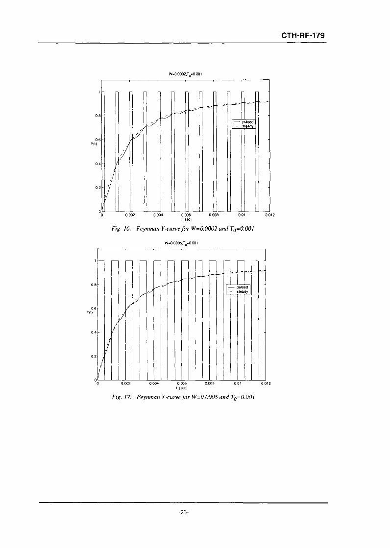
CTH-RF-179
W=00002,T>0 001
OB
0.6Y(t)
0.4
0.2
0 002 0 004 0 006 0.008 0.01 0.012
Fig. 16. Feynman Y-curvefor W=0.0002 and To=0.00I
0.6
06Y(t)
04
0.2
— pulsedslearjy
0002 0006I. (sec|
Fig. 17. Feynman Y-curvefor W-0.0005 and T0=0.001
-23-

CTH-RF-179
W=0 001 .T =0.005
0 6V(t)
1 1 1 — J
/
I
1
1
1 .
I /
/
t 1
//
1/
pulsedsteady
-
0 0 002 0 004 0 006 0.008 0 01 0 012I. laecl
Fig. 18. Feynman Y-curvefor W=0.001 and To=0.005
0 002 0 004 0 006 O.0O8 0.01
Fig. 19. Feynman Y-curvefor W=0.0005 and T0=0.005
-24-

CTH-RF-179
A similar figure, showing the Y-curve for both Gaussian and square pulses is shown inFig. 20 below. It illustrates the already mentioned fact that the Y-curve corresponding to Gausspulse shapes is smoother than its counterpart which is due to square pulses.
0.01
gaussian- - square- steady
0.012
Fig. 20. The resulting Feynman Y-curve for Gaussian and square pulse, included numerical values areW = 0.0005, TQ = 0.005, a = W/4, s = J
-25-

CTH-RF-179
6. Determination of the Parameter a from a Simulated Measurement
It is possible to simulate a measurement using the formulas in Section 3. and adding arandom noise to it, to simulate the imperfect character of an experiment. Using a MATLABroutine, Isqcurvefit, which solves curve-fitting problems in the least-squares sense, it is possibleto estimate the value of a . Figs 21 and 22 show Feynman y-curves with simulatedmeasurements for two different noise levels. In this study only square pulses are assumed, andthe pulse repetition frequency and the pulse width are assumed to be known exactly. In realitythis is not true, and a sensitivity analysis of the unfolding method to inaccuracies in thoseparameters should be also performed, which will be made at a later stage.
The resulting curve for the estimated a is included in the Figures below as well. The truey-curve and the one obtained by the parameter a from the fitting procedure cannot bedistinguished in the figures. In all figures, a 0 denotes the original value and an denotes theestimated value. In Fig. 21 and Fig. 22 the noise level is 4 and 8 percent of the asymptotic valueof the original Feynman- Y curve, respectively.
12
08
Y(t)
0 l
-0.2
•>mdMI iin 1 " W! p| it
" /
a + noise. ao=1053_ an=1052
-
0002 0006I. [sec]
0006 0 01 0012
Fig. 21. Feynman-Y curve for a simulated measurement, the noise level is 4%
In both cases, the true value a 0 was 1053. In the case with lower noise level, the ttn
determined from the curve fitting was 1052, while in the second case an was 1051. However,the precision of the method depends on the level of the added noise and even for the same noisestrength, the particular realisation of the random noise. This is illustrated with the case shown inFig. 23. The noise level is the same as in Fig. 22, i.e. 8 percent, but the estimated a is 1062.
The few cases shown here support the statement that with the formula for thedeterministically pulsed Feynman-alpha measurements, the prompt neutron time constant canbe estimated with curve fitting similarly to the traditional case of constant source. Test of themethod with real measurement data will be reported in a forthcoming publication.
-26-

CTH-RF-179
0 004 0.006t, [sec]
0008 0 01 0.012
Fig. 22. Feynman-Ycurve with simulated noise, the noise level is <
Y(0 a + noisea°=1053a =1062
0 002 0004 0006t. [sec]
0008 0012
Fig. 23. Feynman-Y curve with simulated noise, the noise level is 8%
-27-

CTH-RF-179
7. Conclusions
Calculation of the deterministically pulsed Feynman-alpha formula with the methodintroduced in this report leads to a compact solution which is easy to use in numerical work.One particular advantage, demonstrated in this report, is the ease with which various forms ofthe pulse shape can be handled. All that is needed is a Fourier-series expansion of theasymptotic form of the source induced neutron number. Once the coefficients of this quantityare obtained, they can be substituted into a general formula for the relative variance, which wasderived in the report.
The Feynman formula obtained was investigated quantitatively for various pulseparameters and even shapes. The possibility of using the formula for determining the promptneutron time constant, and through that the reactivity, was investigated in simulations. It wasfound that despite the much more complicated structure of the Feynman y-curve as comparedto that with constant (time-independent) sources, the prompt alpha parameter can be extractedfrom a simulated experiment with methods of parameter fitting.
References
[1] Pazsit I. and Kuang Z.F. Reactivity Monitoring in ADS with Neutron FluctuationAnalysis. Proc. Embedded technical meeting AccApp at the Winter meeting of theAmerican Nuclear Society, Reno, Nevada, 10-15 November 2001
[2] A. Billebaud, R. Brissot, D. Heuer, M. Kerveno, C. Lebrun, E. Liatard, J.M. Loiseaux,B.O. Meplan, E. Merle, F. Perdu, J. Vollaire: The Muse-4 experiment - Prompt reactivityand neutron spectrum measurements. Proc. PHYSOR 2002 - International Conferenceon the New Frontiers of Nuclear Technology: Reactor Physics, Safety and High-Performance Computing. Seoul, Korea, October 7-10, 2002
[3] Pazsit I. Neutron fluctuations in traditional and accelerator driven reactors. Fluctuationand Noise Letters 1, R101-R118 (2001)
[4] Ceder M. and Pazsit I. Analytical solution for the Feynman-alpha formula for ADS withpulsed neutron sources. Prog. nucl. Energy 43, 429 - 436 (2003)
[5] Pazsit I., Ceder M. and Kuang Z. Theory and analysis of the Feynman-alpha method fordeterministically and randomly pulsed neutron sources. To appear in Nucl. Sci. Engng(2004)
[6] Kitamura, Y, Misawa, T., Unesaki, H., Shiroya, S., "General Formulae for the Feynman-Alpha Method with the Bunching Technique", Ann. Nucl. Energy, 27, 1199-1216 (2000)
[7] Kitamura, Y., Yamauchi, H., Yamane, Y, "Derivation of Variance-to-Mean Formula forPeriodic and Pulsed Neutron Source", Ann. Nucl. Energy, 30, 897-909 (2003)
[8] Kitamura, Y, Yamauchi, H., Yamane, Y, Misawa, T., Ichihara, C , Nakamura, H."Experimental Investigation of Variance-to-Mean Formula for Periodic and PulsedNeutron Source", Ann. Nucl. Energy, 31, 163-172 (2004)
[9] I. Pazsit (2002), Transport Theory and Stochastic Processes, Lecture notes, ChalmersUniversity of Technology, Gothenburg, Sweden
-28-

Paper II


Available online at www.sciencedirect.com
toiiHci/g)DiHicT« annals of
^ NUCLEAR ENERGY
ELSEVIER Annals of Nuclear Energy 32 (2005) 986-1007
www.elsevier.com/locate/anucene
Calculation of the pulsed Feynman-alphaformulae and their experimental verification
I. Pazsit a'*, Y. Kitamura b, J. Wright a, T. Misawa c
a Department of Reactor Physics, Chalmers University of Technology, SE-412 96 Goteborg, Swedenb Graduate School of Engineering, Nagoya University, Furo-cho, Chikusa-ku, Nagoya 464-8603, Japan
c Research Reactor Institute, Kyoto University, Kumatori-cho, Sennan-gun, Osaka 590-0494, Japan
Received 6 October 2004; accepted 20 December 2004Available online 31 March 2005
Abstract
An effective method of calculating the pulsed Feynman-alpha formula for finite widthpulses is introduced and applied in this paper. The method is suitable for calculating boththe deterministic and the stochastic Feynman-alpha formulae, while also being capable oftreating various pulse shapes through very similar steps and partly identical formulae. Inthe paper both the deterministic and the stochastic cases are treated for square and Gaussianpulses. The solutions show a very good agreement with the results of currently performedexperiments by some of the authors at the Kyoto University Critical Assembly (KUCA).
The formulae obtained are also used for a quantitative evaluation of the prompt neutrondecay constant from a large number of experiments made at the KUCA for a wide rangeof parameters such as subcritical reactivity, pulse repetition frequency and pulse width. Thesuitability of the formulae to determine the prompt neutron decay constant a by curve fittingto the measured data was investigated. It was found that, despite the larger deviation from thetraditional Feynman y(7)-curves from the traditional ones with a constant source (i.e., largerripples superimposed on a smooth curve), the stochastic pulsing method is superior to thedeterministic one in that it yields the correct a value for all subcriticalities. The deterministicmethod also works fine for most cases, but its application is not so straightforward.© 2005 Elsevier Ltd. All rights reserved.
Corresponding author. Tel.: +46 31 772 3081; fax: +46 31 772 3079.E-mail address: [email protected] (I. Pazsit).
0306-4549/$ - see front matter © 2005 Elsevier Ltd. All rights reserved.doi:10.1016/j.anucene.2004.12.007

/. Pdzsit et al. I Annals of Nuclear Energy 32 (2005) 986-1007 987
1. Introduction
The theory of the Feynman-alpha method with pulsed sources became interest-ing recently in connection with the future accelerator-driven systems (ADS). Cur-rent on-going experimental pilot projects with the aim of studying ADS basics usepulsed neutron generators as a source (Soule, 2001, 2002; Kitamura et al.,2004a,b). Even the spallation sources, planned to be used in a future full-scaleADS facility, might be operated in a pulsed mode, for technical reasons.Although there are several competing methods to be used in pulsed source exper-iments to determine reactivity, most notably the area-ratio method (Sjostrand,1956; Soule, 2001, 2002), the Feynman- or Rossi-alpha methods have always beenconsidered as interesting complements. Hence their applicability and performancehas been a matter of current interest.
In line with the above, formulae for the Feynman-alpha method with pulsedsources have been elaborated in the past few years. Several methodologies to modelthe physical situation have been applied, which differ in the definition of the pulseshape (including Dirac-delta descriptions), and also in how the measurement is eval-uated. With respect to the latter, it is customary to distinguish between deterministicand stochastic data evaluation techniques (Degweker, 2000; Pazsit and Kuang, 2001;Ceder and Pazsit, 2003). These will also be referred to as the "deterministic (stochas-tic) pulsing" or "deterministic (stochastic) Feynman method". They only differ inwhether the counting gate opens in a synchronized manner with the pulsing, or ran-domly. Since the time-to-digital conversion is nowadays made with a high resolution,a measurement consists of the registration of the arrival time of each detector count,such that the neutron pulse trigger is also recorded. Hence a measurement can beevaluated by both the deterministic or the stochastic method.
The first papers on this subject assumed Dirac-delta pulses (Degweker, 2000;Yamane et al., 2000, 2001, 2002; Kitamura et al., 2003, 2004a,b). This methodwas then extended to describe the production of neutrons in a spallation sourcewith Monte-Carlo simulations of the intranuclear cascade (Munoz-Cobo et al.,2001). In another line, finite width pulses were considered, first with squarepulses, such that the neutrons within one pulse were regarded as being indepen-dent (i.e., Poisson-distributed with a time-dependent intensity); however, the caseof exponentially decaying pulses was also considered (Degweker, 2003). Thedeterministic Feynman-alpha formula for square pulses was derived by solvingthe corresponding equations for each pulse in a piecewise manner (Pazsit andKuang, 2001). This method was clumsy in the sense that its extension to morecomplicated (and hence realistic) pulse shapes was not feasible. The stochasticpulsing was then solved with a much more powerful method, using Laplace trans-form and complex function techniques (Ceder and Pazsit, 2003). This techniquewas then applied also to the deterministic case (Pazsit et al., 2004), but its poten-tial was not fully utilized, and the first results were only restricted to the recon-struction of the previous quantitative results of Pazsit and Kuang (2001).
In this paper the solution based on the Laplace transform technique is developedfully by evaluating some integrals explicitly. These were left symbolic and were

988 /. Pdzsit el al. I Annals of Nuclear Energy 32 (2005) 986-1007
evaluated at run-time by Mathematica during each calculation in the predecessor pa-per (Pazsit et al., 2004) for the deterministic case. Such a solution naturally yieldedboth a slow and a non-transparent algorithm. With the integrals evaluated explicitly,we were able to give compact and robust solutions.
One particular advantage is the ease with which various pulse shapes can betreated with very little extra effort. A second advantage is the possibility of givinga common treatment for both the deterministic and the stochastic pulsing in aunified frame. Due to the Gaussian form of the pulse shape (in time) of theGENEPI neutron source used in the MUSE project, the Feynman-formula wasderived with Gaussian pulses, in addition to the square pulses treated alreadyearlier.
That is, altogether four different cases will be treated here: deterministic and sto-chastic pulsing with square and Gaussian pulses. Illustrative cases of the FeynmanY(T) curves are shown, and the results discussed. One significant difference betweenthe deterministic and stochastic case, irrespective of the pulse shape, is that in thelatter, the relative magnitude of the deviations between the pulsed and the tradi-tional case with continuous sources depends on the source strength. No such depen-dence exists for the deterministic case. This important aspect was overlooked so far,but it is confirmed here not only by formulae, but also by experiments. In partic-ular, this circumstance can explain the difficulties in applying the Feynman methodto the MUSE experiments.
The validity and applicability of the formulae was checked by comparisons torecent experiments. Recently, a series of experiments were performed at the KyotoUniversity Critical Assembly (KUCA) (see Kitamura et al., 2004b). The measure-ments were then processed by both the deterministic and stochastic techniques,and the corresponding Y(T) curves were evaluated. These show excellent qualitativeand quantitative agreement with the theoretical curves. The theoretical expressionswere used to evaluate the prompt neutron decay constant from the measurements,and could be compared with the reference values (which were known from the area-ratio method). A very good agreement was found between the reference a valuesand those fitted from the experiments for the case of the stochastic pulsing, forall measurements. With the deterministic method, still good results were obtained,but its application was slightly less straightforward, as it will be described below.The success of the stochastic method here represents a definite change in the assess-ment of the applicability of the two methods, compared to earlier work. In Pazsitet al. (2004), it was judged that the deterministic method is more promising. Thisconclusion was based mostly on application of the theory to MUSE measurements,which had poor statistical quality as compared to the measurements reported on inthis paper.
The comparison and good agreement with experiments can be interpreted as aconfirmation of the basic theoretical approach, even if certain further develop-ment is envisaged. These concern accounting for the fact that neutrons in a shortpulse cannot be treated as fully independent, like it is made in the current methodused. The corresponding development will be given in a subsequent communi-cation.

/. Pdzsit et al. I Annals of Nuclear Energy 32 (2005) 986-1007 989
2. General theory
The principles and the basic theory of the Feynman-alpha method are describedin several publications, including the predecessors of the present work (e.g. in Pazsitand Kuang, 2001; Pazsit et al., 2004). The method is based on the measurement ofthe first two moments of the detector counts Z{T) during a measurement time periodT in a stationary system driven with a source S. (As usual, the tilde indicates that wedeal with a quantity induced by the source, in contrast to the neutron number, detec-tor count, etc. due to one single source particle). The measurement yields the depen-dence of the relative variance, or the variance-to-mean a2^{T)/Z(T) (Feynman-alphafunction) on measurement time. In practice, it is more customary to use the deviationof the relative variance from unity, which is called the Feynman y-function:
where
(Z(Z - 1)) - <Z>2. (2)
is called the modified variance. The purpose of the theory is to serve an explicit for-mula for the Feynman y-function.
Such a formula can be calculated from a master equation, i.e., from a probabilitybalance equation. Usually, it is more advantageous to use the so-called backwardmaster equation, which means that one has to operate on initial variables. In this for-malism, a core with a stationary source is modeled by switching on the source att = 0 rather than at / = —oo, and the measurement is made when / —* oo. For reasonsinherent in the properties of the backward master equation approach, one needs togo in two steps; first the probability of the number of neutrons in the system anddetector counts during the time period {t — T,t) is determined, and then from thisthe probability of the same quantities is calculated for the case of an external source.The joint distribution of observables due to a single particle,
P{N,Z,t), (3)
or its probability generating function,
N=0 Z=0
can be derived directly from a backward equation, and this has been done a longtime ago. Here P is the probability of finding N neutrons at t and Z counts in thetime interval (t — T,t), due to one neutron starting the process at t = 0. As (3) and(4) indicate, we shall neglect the existence of the delayed neutrons in this work. Theywill be treated in a subsequent publication (Kitamura et al., 2005a).
The next step is to derive an expression that connects the distribution of the sameobservables as being due to an external source switched on at t = 0, and those due toa single particle, (3) or (4). Such a relationship can be derived from another master

990 /. Pdzsit et al. I Annals of Nuclear Energy 32 (2005) 986-1007
equation, and its solution has also been known for long. The present authors haveoften referred to the formula as the Bartlett formula, but the formula was knowneven earlier (Sevast' yanov, 1951), as it was pointed out to us recently (Pal, 2004).At the level of the generating functions, it usually reads as
G{x,z,t) =exp [lS{f){G{x,ztt-/)-l}dl!Jo
(5)
The measurement time T is not denoted in the above notation. The formula needs tobe considered in its asymptotic form when t —> oo. In the traditional case of constantsource, this can be made in (5) by extending the upper limit of the integration toinfinity. However, with a non-stationary (periodic) source, this is not possible di-rectly in (5), rather at the level of the various moments when the concrete form ofthe source is defined.
Since we also will discuss the case of stochastic pulsing, the relationship (5) needsto be generalized (Pazsit and Kuang, 2001). This is made by the introduction of arandom variable £ e [0,
G(x,z,t)= / G(jcIz,/|Op(Od{=(G(x,z,r|O>, (6)Jo
where
G(x,z,t\£) = exp \£s(t'\Z){G(x,z,t - t') - 1} dr'j, (7)
and the (• • •> symbol stands for the expectation value w.r.t. £ in (6). The "randomi-zation" of the source means simply that
= S(t - 0- (8)
What regards the source, the pulsed character is formulated mathematically that thepulse train consists of a periodic sum of the same pulse shape ("pulse mother func-tion" in recent wavelet terminology) J{t) such that it is non-vanishing only within[0, To), i.e.,
n 1 <»>0, otherwise.
Here j{t) is assumed to be normalized in some sense, whereas the intensity of thesource will be described by an intensity factor SQ. With this and in view of (9), thesource can be written as
oo oo
S(t) = So ^ f{t - nT0) = So J^Mtl (10)n=0 n=0
and with (8) one has
-nTo-Z). (11)

/. Pdzsit et at. I Annals of Nuclear Energy 32 (2005) 986-1007 991
Various forms of the pulse shape j{t) will be specified later. For the discussion of thesolution technique that follows below, it can be left unspecified. This will exemplifyone advantage of the technique used, namely that it can be applied to various pulseshapes with roughly the same effort, and that a substantial part of the steps does notdepend on the pulse shape. This means that new pulse shapes can be treated with arather moderate extra effort, once the problem was fully solved for one particularpulse shape.
The two different pulsing methods, i.e., deterministic and stochastic, can actu-ally be treated in a common framework by specifying the corresponding probabil-ity distributions of the random variable <!;. For the stochastic pulsing, one willhave
whereas for the deterministic case it is given as
Pit) = &(£)• (13)
From (7) and (13) it is seen that the results of the deterministic case are equivalentwith substituting ^ = 0 into the formulae which contain £, whereas those of the sto-chastic case will require integration over the pulse period (see (12)). This latter canalso be achieved relatively easily, because the kernel functions, over which the inte-grations need to be taken, will be given as a Fourier expansion over the same period.For this reason we will first derive generic results with the dependence on the randomvariable £ retained, from which then the deterministic and stochastic cases can be ob-tained through the procedures described above.
For the Feynman-alpha formula one needs the first and second factorial momentsof the source induced distributions. These are given, from (5) (7), through integralsof the corresponding first two factorial moments of the single particle induced distri-butions. Before the treatment of the concrete cases of deterministic and stochasticpulsings with square and Gaussian pulse shapes, we list the relevant formulae. Thiswill facilitate the overview of the flow of the calculations, and demonstrate also thefact how the various pulse shapes can be treated in a common framework.
The relevant formulae for the moments of the single particle induced distributionscan be summarized as follows. For the first moments one has
(14)
where a is the prompt neutron decay constant, given by —piA. Here - p is the subcriticalreactivity (to be determined in the measurement) and A the prompt neutron generationtime. As indicated in Eq. (14), and in accordance with several previous publications, thenotation (...) for the expectation value is omitted here and from now on for the firstmoment quantities, as long as it does not lead to confusion. Further

992 /. Pdzsit et al. I Annals of Nuclear Energy 32 (2005) 986-1007
, T)) .
where
, T) =1,
.0, t>T.
The second factorial moment M^t, T), defined as
,u Z2G(x,z,t)
dz2x=z=\
is given by
Mz(t,T)= I Qz(t',T)N(t-t')dt',Jo
with
(15)
(16)
(17)
(18)
(19)
where Z(t,T) is the single-particle induced detector count, given in Eq. (15).The corresponding formulae for the source induced factorial moments are ob-
tained from (5) or (6) and (7) as follows. Here, we still keep notations on the randomvariable £, although it can be neglected when treating the deterministic case. Expec-tation values w.r.t. < will be denoted by brackets as in Eq. (6), whereas N and Zstand for the first moments and Mz for the second factorial moment of the corre-sponding random variables. The basic formulae for the first moments are then
N(t) - (N(t\Z)) =jr=r=l
= f'(S(t'\O)N(t-t')d^ (20)Jo
where
and
= ['s(t'\Z)N(t-t')dt\Jo
(21)
= ['(S(t'\Z))Z(t-t'J)dt'Jo
Jo\{t'J)N{t-t')dt\
with
Z(/, T\£) = f S(t'\Z)Z(t - t', T) dt' - Xd f A(t', T)N(t - t'\£) dt'.Jo Jo
(22)
(23)

/. Pdzsit et ai I Annals of Nuclear Energy 32 (2005) 986-1007 993
The reason for the fact that the source induced detector count can be written in twodifferent ways is that it is a double convolution between three different functionswhich, in turn, is due to a commutation relation (Bell, 1965; Mufioz-Cobo et al.,1987). By using previous definitions and expressions, one out of two convolutionscan be re-denoted as an autonomous function/notation, and this can be done bytwo different ways. This dual representation gives a possibility to choose the formthat suits the actual computations better, which fact will be utilized below.
The second factorial moment of the source induced distributions,
= (Z(Z-l)) =\ vz-
can also be expressed in two equivalent ways. For simplicity and later reference, we
give it here before the expected value w.r.t. £ is calculated. One has then
S(t'\Z)Mz(t - t', T) dt' + Z (/, T\Cl
= f Qz(f, T)N(t - if, 0 dt' + Z\t, T\{). (25)Jo
One often uses the modified variance instead, which from the definition (2) and (24)above can be written as
T) = Mz(t,T)-z\t,T). (26)
From the above this leads to
= ['(S(t'\O)Mz(t - /', T) dt' + (Z2(r, T\0) - z\t, T)Jo
= f Qz(t', T)N(t - 0 dt' + (z\t, T\Q) - Z\t, T). (27)Jo
Here the term which is next last in the last two equalities, (Z (/, T\£)}, requires someattention. Its kernel is given by Eq. (23) which has to be squared and then the ex-pected value w.r.t. £ is to be taken. Due to the convolution in (23), it is easy tosee that with the probability distribution as in (12), i.e., the stochastic method, thesquaring and the expectation value w.r.t. £ do not commute, hence the last two termsof (27) will be different. With the distribution of (13), i.e., the case of deterministicpulsing, those two operations commute, just as with a constant source. Hence in thatcase the last two terms of (27) cancel each other, and then again, with neglectingnotation on £, the convolution can be rearranged to
Jiz(t,T)= f's(t')Mz(t-t')dt'= f Qz{t'J)N{t-t')dt\ (28)Jo Jo
with Qz(t, T) being given by (19). This is what is used in principle in the deterministicmethod.

994 /. Pdzsit et al. I Annals of Nuclear Energy 32 (2005) 986-1007
3. General calculation of the variance-to-mean with arbitrary pulse shapes and pulsingmethods
As was seen in the previous section, the task is to calculate the kernelsN(t\£),Z(t, T\£), and with their help the second order quantities Mz(t, T\^) and/or(Jiz(t, T\£)). These need to be obtained for the case t —> oo and then the expectationvalue of these quantities w.r.t. £ needs to be taken. The formal solution for these canbe given for arbitrary pulse shapes, with the pulse shape only affecting certain termsof a Fourier expansion. In this section the pulse will be described by its "motherfunction" fit), as defined in (9).
The starting point is the Laplace transform of Eq. (21), which reads as
N{s\l)=S(s\Z)N(s). (29)
By virtue of (10) and (11) (or (8)) and (14), Eq. (29) can be written as
Here, J[s) is not a full Laplace transform, rather it is defined as
f(s)= p /(/)e-" dr, (31)J
whereas the term (1 - e sT°) in the denominator arises from the summing up of thegeometric series, given rise by the shifted integrals for the terms J\t — nT$). Since thefunction J\s) does not have any singularities of its own, for times / > To, the inversetransform of (30) is entirely determined by the residues of the function
(32)
The actual form of the pulse shape only affects the numerical values of the residues,but not the residue structure, which is as follows:
1. A pole at s = —a, which describes the transient after switching on the source att = 0.
2. A pole at s - 0; the corresponding residue gives the asymptotic mean value of theoscillating function N(t).
3. An infinite number of complex conjugate roots on the imaginary axis at the valuess = ±icon, yielding harmonic functions in the time domain, representing a Fourierseries expansion of the oscillating part of N(t) in the form sin(av) and cos(av).Here the notation
«*=2™ - = 1.2,... (33)
was introduced.
Because we are only interested in the asymptotic values, the terms arising from theresidue at s - — a can be neglected. The residue at s = 0 is simply given as

/. Pdzsit et a!. I Annals of Nuclear Energy 32 (2005) 986-1007 995
_ f(s = O)
whereas Res{icon} + Res{— \oin} can be written as
Res ——^—— + Res ———
= {an sin(ov) + bn cos(av)} cos(ajn£) + {bn sin(av) - a
x sin(con£), (35)
where the parameters an and bn are defined as
2 wnm{niajn)} a3{f(iajn)}an=- 7-—5 , (36)
To co2 + a.2and
2t To o)2 + a2
Then, N(t\^) is given as
(37)
v)} cos(tun0
,,/) - an cos{a),,t)t} sin(wB^)] >. (38)
The actual value of the parameters a0, an and bn will depend on the pulse form. For-mally, however, all subsequent formulae including the variance-to-mean can be cal-culated formally from the above expression.
Eq. (38) shows that in the stochastic case, where averaging w.r.t. t, incur integra-tions of the trigonometric functions over their period, all oscillating terms disappearin N(t), as is expected and as was already shown in previous works. In the determin-istic case the oscillating terms remain present.
For the calculation of the asymptotic value of the detector counts
the last equality of Eq. (23) is the more suitable, by simply integrating (38) term byterm. The execution of the limit t —> oo requires, however, some attention. Since incase of the deterministic pulsing the integrand is oscillating, the limit does not existfor an arbitrary /. However, deterministic pulsing means per definition that the con-dition t = KTQ + T has to be fulfilled, and it is obvious that letting / —> oo equals toletting K —> oo. This procedure is not necessary for the stochastic pulsing, where theasymptotic number of neutrons becomes a constant after the averaging w.r.t. <!;, butfor the sake of uniform treatment, the limit will be calculated for both cases accord-ing to the above. With that, we have:

996 /. Pdzsit et al. I Annals of Nuclear Energy 32 (2005) 986-1007
pKTo+T _ rKTo + T
Z(T\£) = kd / A(t', T)N(t - r ' |0 dt' = kd \ N(t\Q dtJo Jo
= Xd f N(t\Z) dt. (39)Jo
The last step above results from the periodic character of N(t). Performing the inte-gral will yield the result
oo
Z{T\£) = S0Xd[a0T + ^ { t f B ( r ) c o s K O + &tt{T) sin(coBO}], (40)n = l
wherea{\ cos(ojr)} + 6nsin(conr)
- cos(a)nT)} - ansin(o)nr)
This is the general expression for arbitrary pulse shapes and pulsing techniques. Thecase of the deterministic pulsing is then obtained by substituting £, = 0, whereas thestochastic pulsing is obtained by integrating (40) between zero and To w.r.t. £ whichleads to the disappearance of all oscillating parts.
The calculation of the second order moments goes >n similar lines. One finds itagain that, due to the simple explicit expression for N{t\£), it is more convenientto use the last identity of (25) or (28). We shall use here the last equality of (25),where, from (15) and (19), one has
(43)v(v 1 ) ) ( e « r - n V 2 a t , T < t .
As (43) shows, one needs to evaluate the integrals over trigonometric functions mul-tiplied by the zeroth, first and second power of e~°". These integrals can be jointlyevaluated in a formal manner. The execution of the limit t —> oo is performed thesame way as in connection with Eq. (39). After lengthy but straightforward calcula-tions, the result is given in the following form:
S0XdXf(V(v-l))a2
+ (2a)
x Lo^a>ngj ' a2n=\
(2a)- Z2(T). (44)

/. Pdzsit et al. I Annals of Nuclear Energy 32 (2005) 986-1007 997
Here the following notations were introduced:
sfn{T) = Pn(0, T) - 2pn(a, T) + pn(2a, T), (45)
with
sinKQ dt = a ° n W + M e cos(conr)}
Jo «„ + *
and
^ ( 7 ) = qn(0, T) - 2qn(a, T) + qn(2<x, T), (47)
with
fJo
on sin (conT) - a{e~aT - cos (<x>nT)}
co2n + a2 (48)
Eqs. (40)-(42) and (44)-(48), together with (1) and (2), serve as the formal solu-tion for the Feynman-alpha formulae with arbitrary pulse shapes and arbitrary puls-ing statistics. In the following we turn now to the concrete cases. Regarding the pulseshapes, we shall give concrete values of the parameters a0, an and bn for two differentshapes, i.e. square and Gaussian. Regarding the pulsing statistics, the cases of deter-ministic and stochastic pulsings will be treated.
4. Treatment of the pulse shapes and pulsing methods
4.1. Square pulses
The sequence of square pulses is described by
f{t)=H{t)-H{t-W\ (49)
or, through (10), as00
5(0 = So J^ {#(' - nTQ) - H(t - nT0 - W)}, (50)n=0
where H is Heaviside's step function, To the pulse period, and W the pulse width. Inthat case, one has
1 - Q~sfV
f(s)=—1—. (51)
Putting this into (34), (36) and (37) will yield the following results for a0, an and bn:
W
(XI o
a)nsin{a)nW) + a{l - cos(wnW)}r^~,—T\
nn((o2n + a2)
(52)

998 /. Pdzsit et al. I Annals of Nuclear Energy 32 (2005) 986-1007
and
<xsm(o)nfV)-o)n{l-cos(wnW)}nn{(oz
n + a2)
4.2. Gaussian pulses
In this case one has
J S F } (55)and
J 2 J 2 \ [ t nIo) (56)n=Q n=0
where the parameter a has to be chosen such that the overwhelming area of theGaussian falls within the pulse period. A good practical choice is a = WIA. The nor-malization of the pulse shape J[i) was chosen such that the maximum value of thepulse function is unity, i.e., the same as with the square shape. This choice has noother motivation than easy comparison of the two pulse shape forms in the plots.
Strictly speaking, the form (55) does not fulfil the condition (9). One can of courseappend the condition that (55) is valid only for 0 ^ t < To and ihatj{t) is zero other-wise. However, when calculating/^) according to (31), the integration boundarieswill be extended to ±oo, in order to get an analytic result. The error of this approx-imation is very small since f(i) decays very fast outside 0 ^ / < To.
With this, J{s) is given as
= s c J , (57)
where ? = y/lka. Substituting (57) into (34), (36) and (37) yields
«o = - ^ , (58)1X1
<»>

/. Pdzsit et al. I Annals of Nuclear Energy 32 (2005) 986-1007 999
The above two sets of parameters a0, an and bn can now be used in the formulae withdeterministic and stochastic pulsings, derived below.
4.3. Deterministic pulsing
The treatment of the pulsing methods means taking the expected values of theexpressions for the first and second moments of the detector count w.r.t. the randomvariable £. As mentioned earlier and is also seen from (6) and (13), for the determin-istic case this is achieved by substituting £ = 0 into the relevant formulae (40) and(44). This means that the terms containing the s'm(a>n£) terms disappear, and likewisethe last two terms of (44) cancel out. The results for the mean and the modified var-iance will become as follows (for simplicity, the expectation value sign, indicating theaveraging w.r.t. i, will be omitted):
Z(T) = ° 1 - T , \ ^ a»il ~ cos(conr)} + bn s i nKT)— - „ ( 6 1 )
and
_ S Q 4 V ( V ( V - 1 ) ) „ / . 1-e
a,2
X
-aT
a0T[ 1 -aT
A(2«) (62)
The particular cases of square and Gaussian pulses can be then obtained by substi-tuting (52)-(54) or (58)-(60), respectively, into (61) and (62).
Since the Feynman y(7)-function is given as Y(T) = Jiz(T)/Z(T), the sourcestrength S^ cancels out from the formula, similarly as in the case with continuoussources. Since both Z(T) and ^^(T1) are linearly dependent on the measurement timeT, the Y(T) curve goes into saturation, again similarly as in the case with continuoussources. The formulae above also show that the oscillating deviations from the con-tinuous Feynman curve tend to zero asymptotically with the gate time T.
The relative weight of the oscillations depends on the relationship between thepulse angular frequency <x> = IKITQ and the prompt neutron decay constant a. Forthe case co » a, i.e., high pulse repetition frequency, the oscillations are small. Fur-thermore, with increasing pulse width W the relative magnitude of the oscillationsdecreases. For short pulses with low pulse frequency, to ^ a, the deviations fromthe smooth 7(7) become quite significant. The magnitude of the oscillations dependsrather weakly on the level of subcriticality, through the parameter a in the formulae,and it increases with increasing subcriticalites.
The above qualitative analysis is illustrated quantitatively in Fig. 1, which showsdeterministic Feynman Y(T) functions for various pulse frequencies, pulse forms andpulse widths. For comparison, the traditional Feynman y(7)-curves are also shown,designated in the figures as "stationary" (i.e., with a constant source). All curves are

1000 /. Pdzsit et at I Annals of Nuclear Energy 32 (2005) 986-1007
(a)1.2
0.8
^ 0 . 6
0.4
0.2
n
W=0.001,T0=0.002
.7"
L'i
7>
-——~-—
- pulsed- stationary
0.002 0.004 0.006 0.008 0.01 0.012t, [sec]
(b) W=1e06,TQ=0.002
1.2
1
0.8
0.6
0.4
0.2
pulsed— stationary
0 0.002 0.004 0.006 0.008 0.01 0.012t, [sec]
W=0.0005 ,T0=0.002 ,0=0.000125
— gaussian- - • square- - stationary
W=0.0005 ,T0=0.005 ,0=0.000125
0.002 0.004 0.006 0.008 0.01 0.012
t, [sec]
— gaussian— square— stationary
0 0.002 0.004 0.006 0.008 0.01 0.012
t, [sec]
Fig. 1. Theoretical Feynman K-curves for deterministic pulsing, with square and Gaussian pulses.
normalized to the asymptotic values. More illustrative figures for all pulse forms andpulsing methods can be found in Wright and Pazsit (2004).
4.4. Stochastic pulsing
In that case, as (13) shows, one needs to integrate (40) and (44) over the pulse per-iod. Then all harmonic functions disappear in (40), and also the ones seen explicitlyin (44). The only non-trivial case is the integration of the second last term in (44),Z {T\£), which contains second order products of the sine and cosine functions,i.e., requires the evaluation of
ifn = l
(63)
However, substituting the definitions of n and y n , and making use of the orthog-onality relationships between the trigonometric functions, this integral is readilyshown to be equal to

/. Pdzsit et al. I Annals of Nuclear Energy 32 (2005) 986-1007 1001
(«)
Because the expected value of the detector counts is an especially simple smoothfunction for the case of stochastic pulsing, i.e.,
(65)
it is practical to give directly the Y(T) function. It will have the relatively simple form
(66)
Again, the particular cases of square and Gaussian pulses are obtained by substitut-ing (52)-(54) or (58) (60), respectively, into (66). This formula, for the specific caseof square pulses, has been already calculated by Ceder and Pazsit (2003), althoughwith a different and less general solution method which explicitly utilized the prop-erties of the square pulse.
Although the Feynman Y(T) function for stochastic pulsing has hence ap-peared in the literature earlier, some of its important properties were not dis-cussed. One significant difference compared to the deterministic case concernsthe relative weight of the oscillating part to the smooth part. Most notably,the oscillating part is linear in the source strength, that is the source strength doesnot disappear from the relative variance. This is a clear consequence of the "ran-domizing" of the pulse, which leads to a qualitatively different dispersion of thesource neutrons, as remarked in Pazsit et al. (2004); and this property is thentransferred to the statistics of the neutron chain and that of the detector counts.It is interesting that the Diven factor of fission, which is present in all formulaeof the continuous source and deterministic pulsing, is absent from the oscillatingpart of the Feynman formula of the stochastic pulsing. This can be expressed asif the oscillating part is controlled by the source statistics instead of the statisticsof the multiplication of the fission chain.
This also means that with a strong source, the relative oscillations become large.This is presumably the case in the MUSE experiments, where the evaluation of thestochastic Feynman measurements showed a very large oscillating part (Rugamaet al., 2004).
A second feature is that the smooth part of (66) is proportional to I/a2, whereasthe oscillating part behaves approximately as I/a, at least for small pulse widths. Thismeans that the relative weight of the oscillating part will increase with increasingsubcriticalities. This can be interpreted to be a consequence that the oscillating partis influenced mostly by the source properties, whose significance increases in deepsubcritical systems.
Some representative calculated values of the stochastic pulsed Feynman-alphacurves are shown in Fig. 2, to illustrate the above qualitative analysis.

1002
(a)
1
0.8
S0 .6
0.4
0.2
/. Pdzsit et at. I Annals of Nuclear Energy 32 (2005) 986-1007
W=2eO6, TQ=0.02, a=253
— stochastic— stationary
^-rm
0.01 0.02 0.03 0.04 0.05t. [sec]
W=2eO6, T0=0.02. a=494
0.01 0.02 0.03 0.04 0.05t. [sec]
(b)
1
0.8
0.4
0.2
(d)
1.2
1
0.8
0.4
0.2
W=2eO6, T0=0.02, a=369
— stochastic- - stationary
0.01 0.02 0.03 0.04 0.05t. (sec]
W=2eO6, TQ=0.02, a=598
f . . .
— stochastic— stationary
0.01 0.02 0.03 0.04t. [sec]
0.05
Fig. 2. Theoretical Feynman K-curves for stochastic pulsing, with square pulses.
5. Experimental
A large series of Feynman-alpha measurements were made at the KUCA reactor(Kyoto University Critical Assembly) by using a pulsed neutron generator. The mea-surements were made with various subcriticality levels, by various pulse repetitionfrequencies (or periods), and pulse widths. Four subcritical reactivities will be ana-lyzed in the paper, namely 0.65$, 1.30$, 2.07$ and 2.72$, which correspond to alphavalues 266 ± 2 s"1, 369 ± 3 s"1, 494 ± 3 s"1 and 598 ± 4 s"1, respectively. These ref-erence reactivities and corresponding alpha values were determined by the rod dropand the pulsed neutron technique, respectively. The pulse periods To used were about1, 10 and 20 ms. The I/a values varied between 4 and 1.7 ms. Especially with the lon-gest I/a value, the fastest pulsing (1 ms repetition time) led to a Feynman 7-curvewhich did hardly deviate at all from a continuous Feynman curve. Therefore, in thisanalysis only the lowest repetition frequency, corresponding to the 20 ms pulse per-iod, will be discussed. The pulse width used is 2 us throughout. More details of themeasurements can be found in Kitamura et al. (2004b).

/. Pdzsit et al. I Annals of Nuclear Energy 32 (2005) 986-1007 1003
(a) Deterministic method: 0.65$
4.0
3.0
(C)1.2
1.0
0.8
0.6
0.4
0.2
0.0
a (reference) = 266±2s-'a(fitted) = 241±l s1
MeasuredFitted
0.00 0.01 0.02 0.03 0.04
Gate width T [s]
Deterministic method: 2.07$
0.05
a (reference) = 494±3 s1
a (fitted) = 500+2 s-1
0.00 0.01 0.02 0.03 0.04
Gate width T [s]
0.05
(b) Deterministic method: 1.30$
2.0
1.5
B 1.0
(d)1.0
0.8
a (reference) = 369±3s"a (fitted) = 355±ls-i
MeasuredFitted
0.00 0.01 0.02 0.03 0.04
Gate width T[s]
Deterministic method: 2.72$
0.05
a (reference) = 598±4 s 'a (fitted) = 607±4s->
MeasuredFitted
0.00 0.01 0.02 0.03 0.04
Gate width T [s]
0.05
Fig. 3. Measured and fitted results for the deterministic pulsing.
The data could be evaluated both by the deterministic and the stochastic methods.This gave us a possibility to test the above derived formulae both qualitatively andquantitatively, by trying to determine the prompt neutron decay constant with fittingthe above formulae to the measured y-curves. The analysis will be described for thedeterministic and stochastic pulsings below. Corresponding to the known pulseproperties of the neutron generator used, a square pulse form with a widthW - 2 |is was used in the curve fitting.
Fig. 3 shows the measurement results for the four different subcriticality levels forthe case of deterministic pulsing, for the case of To = 20 ms. The experimentally deter-mined Y values are shown as symbols together with the experimental errors, and thefitted curves are shown as continuous lines. These fitted curves were obtained by theleast square fitting calculation where the number of oscillating terms used in the expan-sion was 50. The reference alpha values and the ones obtained from the curve fitting areshown in all four sub-figures. It is seen that for the deep subcriticalities, the fitted values

1004 /. Pdzsit ei al. I Annals of Nuclear Energy 32 (2005) 986-1007
obtain with the reference ones quite well. Correspondingly, the fitted Y(T) curves agreewell with the experimental ones, although they do not coincide completely. With weaksubcriticalities, the fitting procedure yields alpha values and fitted curves that deviatefrom the reference alpha value and measured curve appreciably.
Fig. 4 shows the same cases for the stochastic pulsing. For determining the alpha val-ues, it was found that the least square fitting calculation with the first 10 oscillatingterms was sufficient. It can be seen that both the fitted alpha values and the curves agreewith the reference alpha values and the measured curves quite well, for all subcritical-ities. This is in a sharp contrast with the previous conclusions (e.g., Pazsit et al., 2004)where the stochastic method was judged to be less suitable, due to the larger oscillationsof the Y(T) curve around (or rather above) the continuous one.
The reference reactivity and alpha values, and the fitted alpha values from boththe deterministic and the stochastic pulsings are shown in Table 1.
(a)4.0
0.00
Stochastic method: 0.65$
a (reference) = 266±2 S"1a (fitted) = 253±1 s1
MeasuredFitted
0.01 0.02 0.03
Gate width T [s]
0.04 0.05
Stochastic method: 1.30$
a (reference) = 369±3 s 'a (fitted) = 373±2s"
0.01 0.02 0.03Gate width T [s]
0.04 0.05
(C)1.2
1.0
0.8
0.00
Stochastic method: 2.07$
a (reference) = 494±3 s1
a (fitted) = 495±3s'
0.01 0.02 0.03Gate width T [s]
0.04 0.05
(d)1.0
'Z 0.6
"I0.4
0.2
0.00.00
Stochastic method: 2.72$
a (reference) = 598±4s'a (fitted) = 601 ±4 s1
Measured •Fitted
0.01 0.02 0.03Gate width T [s]
0.04 0.05
Fig. 4. Measured and fitted results for the stochastic pulsing.

/. Pdzsit et al. I Annals of Nuclear Energy 32 (2005) 986-1007 1005
Table 1Measured and reference alpha values for the deterministic and the stochastic methods
Subcriticality ($)
0.65
1.30
2.07
2.72
Pulse period (ms)
20101
20101
20101
20101
Measured <x value (s ')
Deterministic method
241 ± 1 (-9.4%)279 ± 1 (+4.9%)255 ± 1 (-4.1%)
355 ± I (-3.8%)363+ 1 (-1.6%)368 ± 1 (-0.3%)
500 ±2 (+1.2%)476 + 1 (-3.6%)507 ± 3 (+2.6%)
607 ±4 (+1.5%)512 ± 1 (-14.3%)591 ±2 (-1.2%)
(deviation from reference)
Stochastic method
253 ± 1 (-4.9%)262 ± 1 (-1.5%)258 ± 1 (-3.0%)%
373 ±2 (+1.1%)360 ± 2 (-2.4%)367 ± 1 (-0.5%)
495 ± 3 (+0.2%)463 ± 3 (-6.3%)507 ± 2 (+2.6%)
601 ±4 (+0.5%)585 ± 6 (-2.2%)604 ±3 (+1.0%)
Reference value
266 ±2
369 ± 3
494 ± 3
598 1 4
There may be several reasons for the efficiency of the stochastic method. One rea-son for the previous judgement, i.e., that the deterministic method is more applica-ble, was the comparison with the Feynman-alpha measurements in the MUSEproject. Since the MASURCA reactor on which the MUSE measurements are madeis a typical fast reactor core, the I/a values are much smaller, hence only a very fewpulse periods occur before the saturation of the Y(T) curve. Such a case is clearlydisadvantageous for the application of the Feynman method. In the present mea-surements, the pulse repetition frequency is higher in comparison to the alpha value,and the statistics of the measurements is significantly better. It can also be noted thatthe oscillations of the Y(T) curve are smaller in the present measurements than in theMUSE ones (Rugama et al., 2004). This can be explained by the fact, noted in theprevious Section, that the source strength (intensity of the neutron generator) mightbe larger in the MUSE experiments as in the KUCA ones. With the stochastic meth-od, the relative magnitude of the oscillations depends on both the source intensityand the level of subcriticality.
Another circumstance, when comparing the two methods is that, although the oscil-lations of the Feynman 7-curve may be larger (even much larger) for the stochasticmethod than for the corresponding deterministic one, yet the oscillations are quitesmooth. With short pulses, the deterministic curve has sharp "edges", which has theconsequence that far more many terms are needed in the numerical evaluations toreconstruct the deterministic Y function in (61) and (62), than for the stochastic one,Eq. (66). This has also an effect on the accuracy of the curve fitting procedure.
6. Conclusion
The method of solving the backward master equations for the Feynman-alpha incase of pulsed sources proved to be very effective with the technique developed in this

1006 /. Pdzsit et al. I Annals of Nuclear Energy 32 (2005) 986-1007
paper. Various pulse shapes can easily be treated, and it was possible to give a com-mon frame for the derivations in the cases of stochastic and deterministic pulsings.The results showed good agreement with a large range of experiments performed re-cently at the Kyoto University Critical Assembly. Unfolding of the prompt neutrondecay constant by fitting the theoretical expressions to the experimental results waspossible with good accuracy. Despite the larger oscillatory part, and in contrast toearlier judgements and expectations, the stochastic pulsing method proved to be def-initely superior to the deterministic one, regarding the agreement with experimentsand the accuracy of recovering the prompt neutron decay constant.
The flexibility of the algorithm used extends even to the treatment of the Rossi-alpha formula and to the inclusion of delayed neutrons into the formalism. Workhas actually been performed in this direction, and the results will shortly be reportedin forthcoming communications (Kitamura et al., 2005a,b).
Acknowledgments
The authors deeply acknowledge the KUCA staff members including Dr. C. Ichi-hara, Messrs. H. Nakamura, R. Ikegawa, K. Kobayashi, T. Sagane, H. Yamamoto,Dr. C.H. Pyeon, Dr. H. Unesaki, and Professor S. Shiroya for their generous helpand advise. The KUCA experiment was performed under the Visiting Researcher'sProgram at the Kyoto University Research Reactor Institute.
Part of this work was performed when one of the authors (Y.K.) was visiting theDepartment of Reactor Physics, Chalmers University of Technology. Financial sup-port for the visit was supported by the safeguard program of the Swedish NuclearPower Inspectorate.
References
Bell, G.I., 1965. On the stochastic theory of neutron transport. Nuclear Science and Engineering 21, 393.Ceder, M., Pazsit, I., 2003. Analytical solution for the Feynman-alpha formula for ADS with pulsed
neutron sources. Progress in Nuclear Energy 43, 429-436.Degweker, S.B., 2000. Some variants of the Feynman-alpha method in critical and accelerator driven
subcritical systems. Annals of Nuclear Energy 30, 223-243.Degweker, S.B., 2003. Reactor noise in accelerator driven systems. Annals of Nuclear Energy 30, 223-243.Kitamura, Y., Yamauchi, H., Yamane, Y., 2003. Derivation of variance-to-mean formula for periodic and
pulsed neutron source. Annals of Nuclear Energy 30, 897-909.Kitamura, Y., Yamauchi, H., Yamane, Y., Misawa, T., Ichihara, C , Nakamura, H., 2004a. Experimental
investigation of variance-to-mean formula for periodic and pulsed neutron source. Annals of NuclearEnergy 31, 163-172.
Kitamura, Y., Taguchi, K., Yamamoto, A., Yamane, Y., Misawa, T., Ichihara, C , Nakamura, H.,Oigawa, H., 2004b. Application of variance-to-mean technique to subcriticality monitoring foraccelerator-driven subcritical reactor. Paper presented at IMORN-29, Budapest, May 17-19.International Journal of Nuclear Energy Science and Technology (submitted).
Kitamura, Y., Pazsit, I., Wright, J., Yamamoto, A., Yamane, Y., 2005a. Calculation of the pulsedFeynman- and Rossi-alpha formulae with delayed neutrons. Annals of Nuclear Energy (in press).

/. Pdzsit et al. I Annals of Nuclear Energy 32 (2005) 986-1007 1007
Kitamura, Y., Taguchi, K., Misawa, T., Pazsit, I., Yamamoto, A., Yamane, Y., Ichihara, C, Nakamura,H., Oigawa, H., 2005b. Calculation of the stochastic pulsed Rossi-alpha formula and its experimentalverification. Progress in Nuclear Energy (in press).
Munoz-Cobo, J.L., Perez, R.B., Verdu, G., 1987. Stochastic neutron transport theory: neutron countingstatistics in nuclear assemblies. Nuclear Science and Engineering 95, 83-105.
Munoz-Cobo, J.L., Rugama, Y., Valentine, T.E., Michalzo, J.T., Perez, R.B., 2001. Subcritical reactivitymonitoring in accelerator driven systems. Annals of Nuclear Energy 28, 1519-1547.
Pal, L., 2004. Private communication.Pazsit, I., Kuang, Z.F., 2001. Reactivity monitoring in ADS with neutron fluctuation analysis. In:
Proceedings of Topical Meeting on Accelerator Applications/Accelerator Driven TransmutationTechnology Applications '01, Reno, NV, November 11-15.
Pazsit, I., Ceder, M., Kuang, Z., 2004. Theory and analysis of the Feynman-alpha method fordeterministically and randomly pulsed neutron sources. Nuclear Science and Engineering 148, 67-78.
Rugama, Y., Kloosterman, J.L., Winkelman, A., 2004. Experimental results from noise measurements in asource driven subcritical fast reactor. Progress in Nuclear Energy 44, 1-12.
Sevast'yanov, B.A., 1951. Uspekhi Matematicheskikh Nauk 6, 47.Sjostrand, N.G., 1956. Measurements on a subcritical reactor using a pulsed neutron source. Arkiv for
Fysik 11,233-246.Soule, R., On behalf of the MUSE international collaboration, 2001. Experimental validation of the
neutronic characteristics of the sub-critical multiplying medium of an ADS: The MUSE project. In:Proceedings of Topical Meeting on Accelerator Applications/Accelerator Driven TransmutationTechnology Applications '01, Reno, NV, November 11-15.
Soule, R., On behalf of the MUSE international collaboration, 2002. Neutronic studies in support ofADS: The MUSE experiments in the MASURCA facility. In: International Conference PHYSOR2002, Seoul, Korea, October 7-10.
Wright, J., Pazsit, I., 2004. Derivation and analysis of the Feynman-alpha formula for deterministicallypulsed sources. Chalmers Internal Report CTH-RF-179, March.
Yamane, Y., Uritani, A., Ishitani, K., Kataoka, H., Shiroya, S., Ichihara, C , Kobayashi, K., Okajima, S.,2000. Experimental study on reactor dynamics of accelerator driven subcritical system. KURRIProgress Report 1999, vol. 46. Research Reactor Institute, Kyoto University.
Yamane, Y., Uritani, A., Kataoka, H., Nomura, T., Matsui, M., Naka, R., Tabuchi, A., Hayashi, T.,Yamauchi, H., Kitamura, Y., Shiroya, S., Misawa, T., Kobayashi, K., Ichihara, C , Unesaki, H.,Nakamura, H., 2001. Experimental study on reactor dynamics of accelerator driven subcritical system(II). KURRI Progress Report 2000, vol. 53. Research Reactor Institute, Kyoto University.
Yamane, Y., Kitamura, Y., Kataoka, H., Ishitani, K., Shiroya, S., 2002. Application of variance-to-meanmethod to accelerator-driven subcritical system. In: PHYSOR-2002 International Conference on theNew Frontiers of Nuclear Technology: Reactor Physics, Safety and High-Performance Computing,Seoul, Korea, October 7-10.

Paper III


Available online at www.sciencedirect.com
SCIENCE (7~Y\ DIRECT8/ DIRECT® aDHdls ofV ^ NUCLEAR ENERGY
ELSEVIER Annals of Nuclear Energy 32 (2005) 671-692
www.elsevier.com/locate/anucene
Calculation of the pulsed Feynman- andRossi-alpha formulae with delayed neutrons
Y. Kitamura a'*, I. Pazsit b, J. Wright b,A. Yamamoto a, Y. Yamane a
a Department of Materials, Physics and Energy Engineering, Graduate School of Engineering,Nagoya University, Furo-cho, Chikusa-ku, Nagoya 464-8603, Japan
b Department of Reactor Physics, Chalmers University of Technology, SE-412 96 Goteborg, Sweden
Received 16 October 2004; accepted 28 December 2004Available online 25 February 2005
Abstract
In previous works, the authors have developed an effective solution technique for calculat-ing the pulsed Feynman- and Rossi-alpha formulae. Through derivation of these formulae, itwas shown that the technique can easily handle various pulse shapes of the pulsed neutronsource. Furthermore, it was also shown that both the deterministic (i.e., synchronizing withthe pulsing of neutron source) and stochastic (non-synchronizing) Feynman-alpha formulaecan be obtained with this solution technique. However, for mathematical simplicity and thesake of insight, the formal derivation was performed in a model without delayed neutrons.In this paper, to demonstrate the robustness of the technique, the pulsed Feynman- andRossi-alpha formulae were re-derived by taking one group of delayed neutrons into account.The results show that the advantages of this technique are retained even by inclusion of thedelayed neutrons. Compact explicit formulae are derived for the Feynman- and Rossi-alphamethods for various pulse shapes and pulsing methods.© 2005 Elsevier Ltd. All rights reserved.
Corresponding author. Tel: +81 52 789 3775; fax: +81 52 789 3608.E-mail address: [email protected] (Y. Kitamura).
0306-4549/$ - see front matter © 2005 Elsevier Ltd. All rights reserved.doi:10.1016/j.anucene.2004.12.010

672 Y. Kitamura el al. I Annals of Nuclear Energy 32 (2005) 671-692
Nomenclature
Ac=v2.c probability that one neutron is captured per unit time.AfSt;Ef probability that one neutron induces a fission reaction per unit time.XA=vLd probability that one neutron is detected per unit time.v velocity of neutron (constant value).Zc macroscopic cross-section of capture.Zf macroscopic cross-section of fission.£d macroscopic cross-section of detection.p(n,m) probability that n prompt neutrons and m delayed neutron precursors
are generated per one fission reaction.(VP) Y17=oYl™=onP(n'm)> i-e-> first-order moment of number of prompt
neutrons generated per one fission reaction.(vd) Y^oJ2™=omP(n'm)' i-e-' first-order moment of number of delayed
neutrons generated per one fission reaction.(v) <vp)+ (vd), i-e., first-order moment of total number of neutrons
generated per one fission reaction.(VP(VP~1)) YlT=oY^=on(n ~ \)p{n->m)-> i-e-> second-order factorial moment of
number of prompt neutrons generated per one fission reaction.(vpvd) YlT=oY^=onmP{ni m)> i-e-> second-order moment of product of numbers
of prompt neutrons and delayed neutrons generated per one fissionreaction.
(vd(vd~1)) YlT=oJ2™=om(m ~ l)p(«,w), i.e., second-order factorial moment ofnumber of delayed neutrons generated per one fission reaction.
(v(v - 1)) <vp(vp- l)) + 2<vpvd> + (vd(vd - 1)>, i.e., second-order factorialmoment of total number of neutrons generated per one fission reaction.
a ^ , i.e., prompt neutron time constant.X delayed neutron time constant.(1 ^4 , i.e., delayed neutron fraction.p A f ( v ) - ( W A d ) ; j _ e i ) r e a c t i v i t y _
A JJJT, i.e., neutron generation time.
1. Introduction
In recent years, the necessity of determination of the subcriticality in futureaccelerator driven systems (ADSs) has became obvious. Due to technical reasons,ADSs are currently planned to be operated in a pulsed mode, hence the pulsedneutron (or area-ratio) method is expected to be a strong candidate for this pur-pose (Sjostrand, 1956; Simmons and King, 1958). Nevertheless, theoretical andexperimental studies on the Feynman- (or variance-to-mean) and Rossi-alpha (orcorrelation) methods in a pulsed mode have also been pursued, since these methodsare regarded as attractive complements of the pulsed neutron method (Degweker,

Y. Kitamura et al I Annals of Nuclear Energy 32 (2005) 67J-692 673
2000, 2003; Pazsit and Kuang, 2001; Kitamura et al., 2003, 2004, 2005a,b; Cederand Pazsit, 2003; Wright and Pazsit, 2004; Pazsit et al., 2004, 2005; Baeten,2004; Rugama et al., 2004).
In previous papers of the present authors (Pazsit et al., 2005; Kitamura et al.,2005b), an effective solution technique was developed for the calculation of thepulsed Feynman- and Rossi-alpha formulae, based on the Laplace transformand complex function techniques (Ceder and Pazsit, 2003; Pazsit et al., 2004;Wright and Pazsit, 2004). One particular advantage of this technique lies in the fea-sibility of treating various shape functions of the pulsed neutron source. Using thistechnique, only minimum extra calculations are required to take various shapefunctions into account. Hence, if necessary, one can easily derive various formulaefor different shape functions, although the pulsed Feynman- and Rossi-alpha for-mulae for two most probable shape functions (i.e., square and Gaussian) were al-ready given in our previous papers. Furthermore, one finds that the solutiontechnique has yet another advantage in that it provides a common treatment forderiving the formulae for the two variants of Feynman-alpha method, i.e., thedeterministic (or synchronizing) and stochastic (or non-synchronizing) methods(Pazsit et al., 2004, 2005).
However, for mathematical simplicity and the sake of insight, our previousworks were performed in a model without delayed neutrons (Pazsit et al., 2005;Kitamura et al., 2005b). At the same time, it was expected that these advantagesof the solution technique would not be lost by inclusion of delayed neutrons. Themain subject of this paper lies in this point. Namely, the previous treatment wasextended to the case when one group of delayed neutrons is taken into account.This way also the robustness of our solution technique is demonstrated. In thispaper, explicit solutions for the pulsed Feynman- and Rossi-alpha formulae willbe given by rigorously taking the prompt-prompt, prompt-delayed, and de-layed-delayed correlations between prompt and one group of delayed neutronsinto account.
In the following section, calculation of the pulsed Feynman-alpha formula withdelayed neutrons will be described. Calculation of the pulsed Rossi-alpha formulais given in Section 3. In Section 4, specific calculations with respect to squareand Gaussian pulse shapes are performed. The conclusions are summarized inSection 5.
2. Calculation of pulsed Feynman-alpha formulae
2.1. General theory
In Feynman-alpha experiments, neutron counts with respect to a certain gatewidth are repeatedly measured, and the correlation index Y is calculated fromthe mean and variance of the neutron counts thus obtained (de Hoffmann, 1949;Feynman et al., 1956). The Y value is defined as variance-to-mean ratio minusunity, i.e.

674 Y. Kitamura et al. I Annals of Nuclear Energy 32 (2005) 671-692
al(T)
Z(T)1, (1)
where Z(T) and <r~{T) are the mean and variance of neutron counts with respect to agate width T. From the gate width dependence of Y measured for various gatewidths, some important reactor kinetic parameters can be evaluated.
For Feynman-alpha experiments with a pulsed neutron source, two alternativeshave been developed so far, i.e., the deterministic and the stochastic pulsing methods(Pazsit et al., 2004, 2005). In the deterministic method, neutron counting is alwaysstarted so as to synchronize with the pulsing of neutron source. On the other hand,in the stochastic method, this synchronization between the neutron counting andpulsing is not established.
In this section, we will derive the pulsed Feynman-alpha formulae for both thedeterministic and stochastic methods by introducing a solution technique devel-oped by the authors (Pazsit et al., 2005; Kitamura et al., 2005b). The calculationswill be performed by assuming one neutron energy group and a one-point reactorapproximation model throughout; also, one group of delayed neutrons will be rig-orously taken into account. For this goal, a zero-power subcritical reactor systemthat is coupled with a pulsed neutron source is supposed, and the backward mas-ter equation technique for the following probability distribution is utilized (Pal,1958):
P(N,C,Z,T;t); £ £ J>(W,C,Z, 7V) = 1. (2)N=0 C=0 Z=0
Here, P(N,C,Z,T;t) is the probability of finding N neutrons and C delayed neutronprecursors at time t in the system and detecting Z counts in the time interval[t — T,t), due to one initial neutron injected at time t = 0 (see Fig. 1). The masterequation for the probability generating function of P(N,C,Z,T;t), i.e.
G(x,y,z,T;t) = £ !C S A ^ W C,Z, T; /), (3)N=0 C=0 Z=0
is written as
Countinggate
(open) -
(close) •
Zcounts
Time h0 t-T
Fig. 1. Timing diagram for P{N,C,Z,T;t).

Y. Kitamura et al. I Annals of Nuclear Energy 32 (2005) 671-692 675
dG(x,yz,T-t) = _ ( ^ + k + U)G(X^ T. t) + (Ac+/id)
/t=0 m=0
(4)
where Ac is the probability that one neutron is captured per unit time, Af the proba-bility that one neutron undergoes a fission reaction per unit time, A the probabilitythat one neutron is detected per unit time by a neutron detector, A the delayed neu-tron time constant, and p(n,m) the probability that n prompt neutrons and m delayedneutron precursors are emitted in one fission reaction (Pazsit and Yamane, 1999).The function &(T;t) in the last term of Eq. (4) is defined as
A(ri«) = ( 1 ' 0 < ' ^ ' (5)
This function is introduced to express the status of the counting gate, i.e., the num-ber of neutrons captured by the neutron detector are registered when A(T;t) isequal to unity. Eq. (4) will be differentiated to derive single-particle induced mo-ments later.
The backward master equation technique usually involves also anotherprobability
P(N,C,Z,T;t,t0), (6)
which is the probability of having N neutrons and C delayed neutron precursors inthe system at time / and Z counts in the time interval [t — T,i), due to an extraneousneutron source switched on at time t = t0. Introducing the corresponding probabilitygenerating function,
G{x,y,z,T;t,t0) = J2Y1 E A ^ W C,Z, T; t,t0), (7)N=0 C=0 Z=0
one obtains the so-called "Bartlett formula" (that was originally derived by Sevas-t'yanov in 1951) that connects the single-particle induced probability generatingfunction with the source-induced one (Pazsit, 1999; Sevast'yanov, 1951):
G(x,y,z,T;t) = exp ['di!S{S){G{x,y,z,T;t-S)-l}Jo
(8)
where S(t) is the intensity of extraneous neutron source. Here, the notation on t0 wassuppressed, since substitution of t0 = 0 was carried out in deriving Eq. (8). To expressthe periodic nature of source intensity S(t), the pulse shape function of pulsed neu-tron source J{t) that is non-vanishing only within 0 / < T Q is introduced, and withits help the pulse train can be written as

676 Y. Kitamura et al. I Annals of Nuclear Energy 32 (2005) 671-692
-nT0). (9)
Here, So is the source intensity factor (constant value), and To the pulse period. Theuse of the parameter So makes it possible to normalize the pulse shape functionarbitrarily.
In this section, to discuss both the deterministic and stochastic types of the pulsedFeynman-alpha formulae, a generalized expression of Eq. (8) is employed (Cederand Pazsit, 2003; Pazsit et al., 2004, 2005). This generalization is made by introduc-ing a random variable £ (0 ^ £ < To):
G(x,y,z,T;t)= f ° &&{Z)G{x,y,z, T;t\£), (10)[o
with
G(x,y,z, T;t\O = e x p l Y ' d f ' S ^ 1 | Z){G(x,y,z, T;t- t') - 1}] . (11)
The modified source intensity S{t\£) is simply denned asS(t\Z)=S{t-£). (12)
The treatment of the two different experimental methods will be realized by spec-ifying the probability distribution /?(£). For the deterministic method, one will set
p(£) = 5(£); [deterministic method], (13)with
t = kT0 + T; * = 0 , l , - - - , (14)whereas for the stochastic method,
p(£) =—; [stochastic method]. (15)T
2.2. Single-particle induced moments
As mentioned above, one can calculate the single-particle induced moments bydifferentiating G(x,y,z,T;t). Here, for the later reference, the following moments willbe prepared:
dG(x,y,z,T;t)OO 00 OO
Z(T; 0 - E E E ZP^' C'Z' r' 0 ==o c=o z=o
oo oo oo r\2t
(16)x=y—z—1
-i)Wc,z,r;0 = - G ( W i r : / )
=0 c=o z=o dz2
(17)
By substituting x = y = z - 1 after differentiating Eq. (4) with respect to z, one ob-tains the following equation for the first-order moment Z(T;t):

Y. Kitamura et al. I Annals of Nuclear Energy 32 (2005) 671-692 677
dZ(T-t) XB f „ J,j = —OL/,{1 ,t) -\ / GlZ{l,l)C ' + / d A ^ i , t j , ( 1 o J
where the definitions of a, /J, and A are listed in Nomenclature. Using the initial con-dition of Z(T;t), i.e.
Z(r ;0)=0, (19)
one obtains the temporal Laplace transform of Eq. (18) as
AT-,,) = W,,)^ + j ; ^ _ ^ , ^A(r;,) E -it-, (20)
with
(a + A)/I + ^/(a + A)2^2 +
r or
y=p,d /
(a + X)A - \/(a + X)2A2 + 4XApW , ^ ( 2 2 )
^-f^f-; y = P,d; / / ; . (23)a; - ay-
Here, ap and ad are the roots of the inhour equation,s2 + (a + X)s - ^- = 0. (24)
Hence, with the definition1
Aj
one obtains the solution of Eq. (18) as
t). (26)
Performing the integral in the above equation, one obtains the result
<• ' ' I •, T — \ A , I n.T I S - — rt.t T-i . . ^ '
1 It is easily seen that N(s) is the temporal Laplace transform of the single-particle induced neutronnumber N(t), which also serves as the Green's function of the mean and higher moments of the detectorcounts.
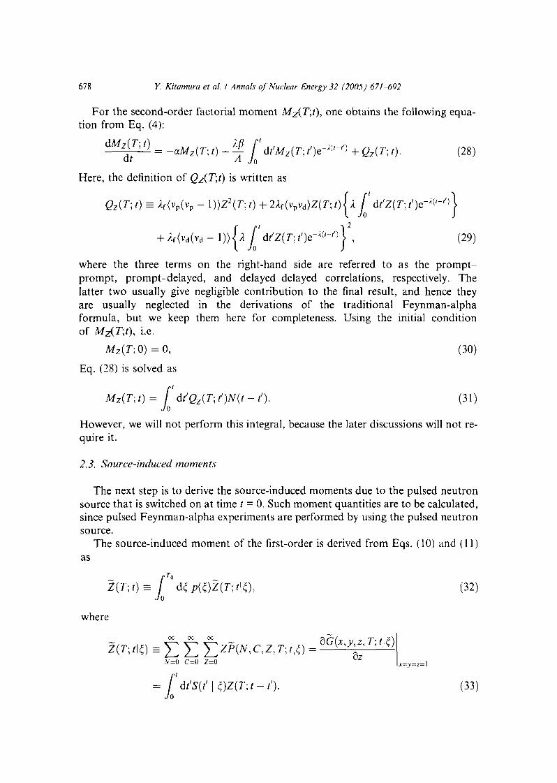
678 Y. Kitamura et al. I Annals of Nuclear Energy 32 (2005) 671-692
For the second-order factorial moment Mz(T;t), one obtains the following equa-tion from Eq. (4):
dM2(T;t) ^ f dt'A Jo
= -o>Mz(T;t)+^- / dt'Mz(T;t')e-"['-n+Qz(T;t)- (28)dt
Here, the definition of Qz(T;t) is written as
Qz(T;t) = Xf{vp(vp- l ))Z2(r;0 + 2Af{vpvd)Z(7;0<A / d/'Z(r,r')e" ; ( '"0 \I Jo J
(29)
where the three terms on the right-hand side are referred to as the prompt-prompt, prompt-delayed, and delayed-delayed correlations, respectively. Thelatter two usually give negligible contribution to the final result, and hence theyare usually neglected in the derivations of the traditional Feynman-alphaformula, but we keep them here for completeness. Using the initial conditionof Mz(T;t), i.e.
Mz(T;0)=0, (30)
Eq. (28) is solved as
Mz(T;t)= fdt'Qz(T-t')N(t-t'). (31)Jo
However, we will not perform this integral, because the later discussions will not re-quire it.
2.3. Source-induced moments
The next step is to derive the source-induced moments due to the pulsed neutronsource that is switched on at time t = 0. Such moment quantities are to be calculated,since pulsed Feynman-alpha experiments are performed by using the pulsed neutronsource.
The source-induced moment of the first-order is derived from Eqs. (10) and (11)as
(32)Jo
where
6G(x,j,z,7V|£)oo oo oo
(V=0 C=0 Z=0
fJo
' dt'S(t'\Z)Z{T-t-t'). (33)

Y. Kitamura et al. I Annals of Nuclear Energy 32 (2005) 671-692 679
Because of the above expression being a double convolution, the temporal Laplacetransform of Eq. (33) becomes
\£) = S(s\Z)Z(T;s) = ldA(T;s)S(s\Z)N(s), (34)
where S(s\£) is the temporal Laplace transform of the source intensity S(t\£) and iswritten as follows (Pazsit et al., 2005):
Here, J{s) is not a full Laplace transform, rather it is denned as
f(s) = fT°dte-slf(t). (36)Jo
Hence, if one uses
-iL., (37)
Eq. (33) is solved as
Z(T; t\£) = Ad / ' dt' &(T; t')N(t - f | 0 - (38)
The Laplace inversion of Eq. (37) is readily obtained by calculating three kinds ofresidues at s = 0, s = —<xj (j = p,d), and s = ± 2nn/T0 (n = 1,2,...) (Ceder and Pazsit,2003; Pazsit et al., 2004, 2005). By taking t > W+ £, the inversion is given as follows(Pazsit et al., 2005):
y=p-d
3nsin(av) + bn<
+ {bn sin(co,,0 - an cos(con/)} sin(co^)], (39)
with
2«7l . _
To '(40)
2 ^ Q i .W{/( j i a ) < , ) } a p { / ( J ia)<,)}-
" = ^ ^ ?T^ ' » - l > 2 , - - - , (41)
fl = ^ ; ^ T ^ ; "-1'2'- (42)

680 Y. Kitamura et al. I Annals of Nuclear Energy 32 (2005) 671-692
Therefore, by substituting Eq. (39) into Eq. (38) and taking T< t, one obtains
y=p,d J
{Vn(T; t) c o s K O + <?n(T; t) sin(co^)}, (43)
where
,* ,T \ - a"fcos { ^ ~ r ) } ~ cos(conr)] 6n[sin {wn(t - T)} - sin{o)nt)}vn\i\t) = ;
w = 1 , 2 , - - - , (44)
frn[cos{a),,(/ - 7)} - cos(con0] an[sin {coB(/ -
(On
n = l , 2 , - - - _ (45)
For the calculation of asymptotic value of Z(T,t), one has to evaluate theexpression
Z(T) = lim Z(T-1) = f ° d^ p(Z)Z(T\Z), (46)J 0
where
. (47)
From Eq. (43), one obtains
= Q) r + Ad50 £ {^(r) cosCw ) + yn{T) sinKO}-
(48)
Here, to calculate ^ n (7) and ^ n ( r ) that are the asymptotic values of <gn{T\t) and£fn{T\i), we took the limit for k -^ oo after substituting Eq. (14) into Eqs. (44)and (45):
= lim Vn(T; kT0 + 7) = ^ ' C O S ( Q > " 7 ' ) > + &" S i n ( " " r ) , (49)
^ lim ^ ( r ; ^ o + D = M l C 0 S ( " n n } fl"sin^"7). (50)
In the following subsection, specific expressions of Z(T) for the deterministic andstochastic methods will be given.
The asymptotic value of the source-induced moment of the second-order is de-rived from Eqs. (10) and (11) as
MZ(T)= [ °dSp(S)Mz(T\Z), (51)
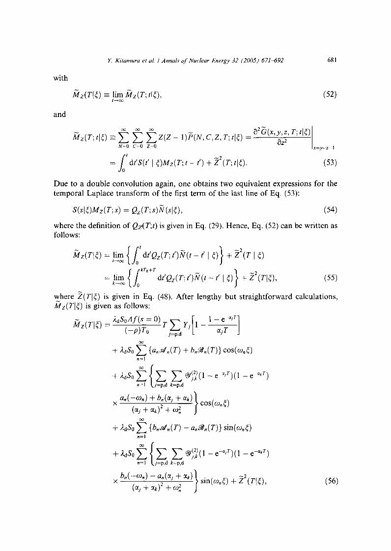
Y. Kitamura et al. I Annals of Nuclear Energy 32 (2005) 671-692 681
with
and
t->00(52)
oo oo oo d2G{x,y,z,T;
=0 C=0 Z=0 x=y=z=\
(53)
Due to a double convolution again, one obtains two equivalent expressions for thetemporal Laplace transform of the first term of the last line of Eq. (53):
S(s\£)Mz(T;s) = Q (T\s)N(s\^) (54)
where the definition of Qz{T;t) is given in Eq. (29). Hence, Eq. (52) can be written asfollows:
**•* L
MZ(T\£) = lim / dt'Qz(T;t')N(t - t' \ £) + Z (T | 0t->oc /o
rkT0 + T _
= lim { I dt'Qz(T; t')N(t ~t'\Q\ + ~Z\T\£)y (55)
where Z(T\£) is given in Eq. (48). After lengthy but straightforward calculations,is given as follows:
^ 0 , 1 / ( 5 = 0 ) „ x - v ! _ .
sin(co^)n=\
(56)

682 Y. Kitamura et al. I Annals of Nuclear Energy 32 (2005) 671-692
where
y=p,d
apad
. - n\ fr
=p,d /t=p,d
v?i«n{*j + «*,n, (59)
m
a/(a ; - a/)
(vpvd) \X ( v ( v - l ) ) A2
(vp(vP-!)>]«; (v p (v p - l ) )a ;2
(61)
.S.^iiilLLJssLlMi^-1" ;2
^ i
- 1)) / \«y a*/ (VP(VP - 1)) ay
*'# *, (62)
- cos{conT)}, (63)
_ consin(conr)- a{e-a7" - cos(conT)}q^,T)= -^-^ . (64)
n
Specific expressions of MZ{T) for the deterministic and stochastic methods will begiven in the following section.
2.4. Treatment of the two pulsing methods
As mentioned earlier, one particular advantage of the solution technique used inthis paper lies in a common treatment for deriving the respective formulae for thedeterministic and stochastic Feynman-alpha methods (Pazsit et al., 2005). This sub-section will be devoted to confirm this feature of the present solution technique.
By ^substituting Eqs. (13) and (48) into Eq. (46), one obtains the first-order mo-ment Z(T) for the deterministic method,
Z(T) = AiS°,*riT °> T + AdS0 V <8n{T)\ [deterministic method], (65)\P)T ^
whereas that for the stochastic method is obtained by substituting Eq. (15) instead ofEq. (13) as

Y. Kitamura et al I Annals of Nuclear Energy 32 (2005) 671-692 683
Z(T) = AdSoAf{-" = 0 ) T- [stochastic method]. (66)
As could be expected, these expressions show a very close similarity to their coun-terparts without delayed neutrons that were obtained in our previous paper (Pazsitet al., 2005), and formally even a complete equivalence. The case of the stochasticmethod is exactly equivalent, while, for the deterministic method, Eq. (65) is also for-mally equivalent to its counterpart with no delayed neutrons. Further, even the def-inition of the quantity ^n{T) in Eq. (49) is formally equivalent to the case of nodelayed neutrons (i.e., Eq. (41) in Pazsit et al., 2005) with the difference that in thepresent case, the coefficients an and bn, i.e., Eqs. (41) and (42), consist now of twoterms, the prompt and delayed terms.
On the other hand, by substituting Eqs. (13) and (56) into Eq. (55), one obtainsMz(T) for the deterministic method as
{y y+ Z (T) [deterministic method], (67)
where Z(T) is that of the deterministic method, i.e., Eq. (65). Furthermore, for thestochastic method, the following result is obtained:
+ 2X]S2Q ^2 a"+
2 " s i n 2 ( y T); [stochastic method], (68)
where Z(T) is that for the stochastic method, i.e., Eq. (66). Therefore, using
a~(T) = M?(T)— Z2(T)-\-Z(T) (69)
the respective Feynman-alpha formulae are finally calculated from Eq. (1) as follows:
W/( , = o) / _Z(T)(-p)T0 ^A V
[deterministic method],

684 Y. Kitamura el al. I Annals of Nuclear Energy 32 (2005) 671-692
where Z(T) must be that of the deterministic method, i.e., Eq. (65), and
Y(T) - T Y(\
[stochastic method]. (71)
The formal similarity with the case of only prompt neutrons is again clear and thegeneralization for the inclusion of delayed neutrons is clearly seen in the above for-mulae. For instance, in the both cases (i.e., the deterministic and stochastic meth-ods), the Feynman y-function, corresponding to a static source but now alsoincluding delayed neutrons, can be recognized as one term or factor in the expres-sions above. Like in the case with no delayed neutrons, the stochastic case is givenas a traditional Feynman y-function plus an added non-negative oscillating modu-lation, such that the traditional Feynman y-function constitutes a lower envelope ofthe stochastically pulsed formula. In the case of the deterministically pulsed formula,the modulation is oscillating around zero, hence the traditional Feynman y-functionis confined in the oscillating one of the deterministically pulsed formula.
3. Calculation of pulsed Rossi-alpha formula
3.1. General theory
In (OrndofTs type) Rossi-alpha experiments, the prompt behavior of neutron fis-sion chains in a subcritical nuclear system is directly observed by measuring the timedistribution of neutron pulses following every triggering pulse (Orndoff, 1957).According to the traditional definition, the formula for this distribution, i.e., theRossi-alpha formula, is obtained as the ratio of the two-point (in time) neutrondetection probability f*-2\t\,t2)dt\dt2 to the one-point neutron detection probabilityF*l\t\)dti. The latter is the probability that one neutron is detected in an infinitesi-mal time interval dt\ around t\. On the other hand, F^2\t\,t2) dt\dt2, that is often re-ferred to as the compound neutron detection probability (de Hoffmann, 1949),means the probability that one neutron is detected in dtx around t\ and another neu-tron is detected in dt2 around t2. Therefore, to derive the Rossi-alpha formula, onehas to introduce the master equation technique for a two-point distribution (Pazsitand Yamane, 1999; Kitamura et al., 2005b):
dG(x,y,zuTuz2,T2,x\t) _ + x + X )G(x z T z T v t) + (X 4- X )dt
DO OO
\TX,Wl)KJ \X^yyZ\ , I i ,Z2, / 2t Ti *)
n=0 m=0
x
(72)

Y. Kitamura et al. I Annals of Nuclear Energy 32 (2005) 671-692 685
Countinggate
Time
(open) -
(close) —
0 t - T
counts
! - r t--T t -
M T
counts
T2 r
Fig. 2. Timing diagram for P(N,C,ZuThZ2,T2,x;t).
where G(x,y,Z],Tuz2,T2,r,t) is the single-particle induced generating function of theprobability P(N,C,Z\,TuZ2,T2iT, t). This latter, in turn, is the probability of findingN neutrons and C delayed neutron precursors at time t and Z\ and Z2 counts inmutually non-overlapping time intervals [t— Tt—z5^\,t-xdi^) (/= 1,2) due to one ini-tial neutron injected at time t = 0 (see Fig. 2). The functions for describing the count-ing gates, i.e., A,{r,;/), are defined as follows:
1 = 1 , 2 . (73)
On the other hand, the Bartlett formula for the two-point distribution is writtenas (Pazsit, 1999):
G(x,y,zl,Tl,z2,T2,x;t)= f d£ p(Z)G(x,y,zu Tuz2, T2, T;Jo
= ±- f °dZG(x,y,z],T],z2,T2,T;t\O,^o Jo
(74)
with
G{x,y,zx,Tx,z2,T2,x;t\Z) = ,y,zu Tuz2, T2,x;t - f) -
(75)
Here, G(x,y,z\,T\,z2,T2,x;t) stands for the source-induced generating function ofthe probability P(N, C,Z\,T],Z2, T2, T; t), which is the probability of finding N neu-trons and C delayed neutron precursors at time t and Z\ and Z2 counts in mutuallynon-overlapping time intervals [t—Ti—xdit\,t—xdit\) (i= 1,2) due to an extraneousneutron source being switched on at time t = 0. We have to note here that the syn-chronization between the neutron counting and pulsing of neutron source is notestablished in pulsed Rossi-alpha experiments, so that substitution of />(£) = \/T0,i.e., Eq. (15), was performed into Eq. (74).

686 Y. Kitamura et al. I Annals of Nuclear Energy 32 (2005) 671-692
3.2. Single-particle induced moments
With regard to the pulsed Rossi-alpha formula, the following single-particle in-duced moments will be prepared:
OO CXI OO 00
> ' Z 2 ' r 2 ' x ;
N=0 C=0 Z,=0 Z2=0
dG(x,y,z],T],z2, T2,x;t)
6z,(76)
OO OO OO 00
=0 Z,=0 Z2=0
i 9z2
(77)
By substituting x - y - z\ - z2 = 1 after differentiating Eq. (72) with respect to zt, oneobtains the equation for Z,(r,;r),
dZ,(r,;Qd/
(78)
Because of the initial conditions, i.e., Z, (r,;0) = 0, this equation is readily solvedwith the result
i= 1,2, (79)
where the definition of N(t) is given in Eq. (25). Hence, performing the integral in Eq.(79), one obtains the following results:
Z,(Tl-t) =
t ^ T.<5i,i,
), r,(80)
On the other hand, for the second-order factorial moment M7_^z2{T\,T2,x;t), oneobtains
;t) , A^-=-OLMZlz2{T\,T2,T,t)+—
(81)

Y. Kitamura et al. I Annals of Nuclear Energy 32 (2005) 671-692 687
where
+ Af(vpvd)Z2(r2;0JA J'dt'Z^Tut')^1-'^
^ ^ s O e - ^ 0 } . (82)
Hence, the initial condition MZ{Zl{T\, T2,z;t) = 0 yields the solution of Eq. (81) as
M 2 l Z 2 ( r 1 , r 2 ,T ; r )= / dt'QZxZi{TuT2^t')N{t-t'). (83)Jo
However, again, we will not need to perform this integral.
3.3. Source-induced moments
From the Bartlett formula, the first-order source-induced moments are derived as
TQ JO
whereOO OO OO 00
N=0 C=0 2,=0 Z2=0
dG(x,y,Zi,Tuz2,T2,x;t\O
= ['d/S(t'\t)Zl{Tl;t-l'y, i = l , 2 . (85)Jo
By virtue of a double convolution and the definition of N(s\£) in Eq. (37), Eq. (85)can be re-written as follows:
Zi(Tr,t\Q = Aa / dt'Ai(Tr,t')N(t-t' | 0 ; i = 1,2, (86)
where A^(/|^) is given in Eq. (39). The solutions for Tt + zdit\ < t are hence obtainedas follows:
Zj(Tj]t\£) — Z{Ti\t — T6J}\ I £); / = 1,2, (87)
where Z(T; t\£) is given in Eq. (43). Therefore, the asymptotic values of Z,(r,; t) arecalculated as
688 Y. Kitamura et al I Annals of Nuclear Energy 32 (2005) 671-692
M) = limZ,(r,;O = lim U
= 0)h /=1 ,2 . (88)
As mentioned above, since /^(fijdfi stands for the one-point neutron detectionprobability that one neutron is detected in dt\ around t\, one obtains the followingresult:
, ( , ) ^ l ^ , (89)Furthermore, from the Bartlett formula, the asymptotic value of the second-order
moment, MZlz2(T\,T2,x), is calculated as
1 o Jo
— / d£ MZtZ2(T\,T2,x;t\£) >, (90),^o Jo J
with
MZ]Z2{TuT2,r,t\Z)= / dt'S{t'\it)Mzlzl{Tl,T2,T;t-tl) + Zi(TiJoft ~
Jo(91)
Since P^2){t\,t2) dt\dt2 means the probability that one neutron is detected in d?[around t\ and another neutron is detected in dt2 around t2 = t\ + x, it is obtainedby letting 7, -» 0 and r 2 - • 0 in Eq. (90):
P(2)(/i,/2)dr,d/2 = lim AfZlz2(Fi, T^.T)- (92)
After a lengthy but straightforward calculation with Eqs. (39), (43), (82), and (90),one obtains
(93)n=l
where Yj are identical to those defined in Eq. (57). Therefore, using the probabilitiesgiven in Eqs. (89) and (93), the pulsed Rossi-alpha formula, R(x)dr, becomes asfollows:

Y. Kitamura et al. I Annals of Nuclear Energy 32 (2005) 671-692 689
" T ) d t ' ( 9 4 )
where dt2 was replaced with dr. As could be expected again, this expression showsa very close similarity to that obtained in our previous paper (Kitamura et al.,2005b).
4. Treatment of pulse shapes
In Eqs. (70), (71), and (94), we have derived the pulsed Feynman- (the determin-istic and stochastic) and the Rossi-alpha formulae, respectively. However, specificparameters that depend on the pulse shape function j\t) have not been determinedyet. Hence, in this section, the parameters for the two most probable shape func-tions, i.e., square and Gaussian, will be calculated to demonstrate the feasibility oftreating various shape functions of pulsed neutrons.
The sequence of square pulses is described by the pulse shape function
f(t)=H(t)-H(t-W), (95)
where H{i) is the Heaviside's step function and W the pulse width. In that case, onehas
/
To roc | _ ~sW
dt e~s'f{t) = dt e~slf{t) = . (96)
Jo s
Hence, the specific parameters for square pulses are obtained as follows:f(s = Q) = W, (97)
y=p,d
(100)
On the other hand, when the pulse shape is expressed as the Gaussian function,one can use
(101)

690 Y. Kitamura et al. I Annals of Nuclear Energy 32 (2005) 671-692
where a is a parameter for the width of Gaussian pulses. In that case, the temporalLaplace transform of j\t) is given as
/•7"o r°c
f{s) = / dt e-s'f{t) « / dt c~s'f(t) =J0 J-oo
*W-'e\ (102)
where W = \/2na. It is to be noted here that the boundaries of the above integralwere extended to ± oo to obtain an analytic result. However, the error ofthis extension is very small, since the pulse shape function J\t) decays very fast(Pazsit et al., 2005). Hence, the parameters for Gaussian pulses are obtained asfollows:
f(s = 0)=W, (103)
+ c o n c o s ( y J F ) } ; n = l , 2 , - - - ,
(104)
W 1 — rn sin I - W l !• n — 1 9 . . .
(105)
j , &
5. Conclusion
In this paper, by using a solution technique developed by the authors (Pazsit et al.,2005; Kitamura et al., 2005b), derivation of the pulsed Feynman- and Rossi-alphaformulae was performed by explicitly taking the prompt-prompt, prompt-delayed,and delayed-delayed correlations between prompt and one-group delayed neutronsinto account.
Through derivation of these formulae, the following two advantages of this solu-tion technique were demonstrated:
1. The solution technique can easily incorporate various shape functions of thepulsed neutron source into the pulsed Feynman- and Rossi-alpha formulae.
2. The solution technique can provide a common treatment for deriving the formu-lae for the two versions of the pulsed Feynman-alpha method, i.e., the determin-istic (i.e., synchronizing with the pulsing of neutron source) and stochastic(non-synchronizing) methods.
Y. Khamura et al. I Annals of Nuclear Energy 32 (2005) 671-692 691
These two advantages are identical to those demonstrated through our formalderivations that were performed in a model without delayed neutrons (Pazsitet al., 2005; Kitamura et al., 2005b). The present treatment shows that these advan-tages are retained even if delayed neutrons are accounted for. Compact explicit solu-tions were derived for various pulse shapes and pulsing methods.
Some comparison with measurements, and the use of the formulae for evaluatingpulsed Feynman-alpha measurements will be given in another forthcomingpublication.
Acknowledgements
This work was performed when one of the authors (Y.K.) was visiting the Depart-ment of Reactor Physics, Chalmers University of Technology in Sweden.
Financial support for the visit was supported by the safeguard program of theSwedish Nuclear Power Inspectorate.
References
Baeten, P., 2004. Heuristic derivation of the Rossi-alpha formula for a pulsed neutron source. Annals ofNuclear Energy 31, 43-53.
Ceder, M., Pazsit, I., 2003. Analytical solution for the Feynman-alpha formula for ADS with pulsedneutron sources. Progress in Nuclear Energy 43, 429-436.
de Hoffmann, F., 1949The Science and Engineering of Nuclear Power, vol. 2. Addison-Wesley, Cambridge(Chapter 9).
Degweker, S.B., 2000. Some variants of the Feynman alpha method in critical and accelerator driven subcritical systems. Annals of Nuclear Energy 27, 1245-1257.
Degweker, S.B., 2003. Reactor noise in accelerator driven systems. Annals of Nuclear Energy 30, 223-243.Feynman, R.P., de Hoffmann, F., Serber, R., 1956. Dispersion of the neutron emission in U-235 fission.
Journal of Nuclear Energy 3, 64-69.Kitamura, Y., Yamauchi, H., Yamane, Y., 2003. Derivation of variance-to-mean formula for periodic and
pulsed neutron source. Annals of Nuclear Energy 30, 897-909.Kitamura, Y., Yamauchi, H., Yamane, Y., Misawa, T., Ichihara, C , Nakamura, H., 2004. Experimental
investigation of variance-to-mean formula for periodic and pulsed neutron source. Annals of NuclearEnergy 31, 163-172.
Kitamura, Y., Taguchi, K, Yamamoto, A., Yamane, Y., Misawa, T., Ichihara, C , Nakamura, H.,Oigawa, H., 2005a. Application of variance-to-mean technique to subcriticality monitoring foraccelerator-driven subcritical reactor. International Journal of Nuclear Energy Science and Technol-ogy (submitted).
Kitamura, Y., Pazsit, I., Wright, J., Misawa, T., Taguchi, K., Yamamoto, A., Yamane, Y., Ichihara, C,Nakamura, H., Oigawa, H., 2005b. Calculation of the stochastic pulsed Rossi-alpha formula and itsexperimental verification. Progress in Nuclear Energy (submitted).
Orndoff, J.D., 1957. Prompt neutron periods of metal critical assemblies. Nuclear Science and Engineering2, 450-460.
Pal, L., 1958. On the theory of stochastic processes in nuclear reactors. II Nuovo Cimento 7 (Suppl.), 25-42.
Pazsit, I., 1999. The backward theory of stochastic particle transport with multiple emission sources.Physica Scripta 59, 344-351.

692 Y. Kitamura el al. I Annals of Nuclear Energy 32 (2005) 671-692
Pazsit, I., Ceder, M., Kuang, Z.F., 2004. Theory and analysis of the Feynman-alpha method fordeterministically and randomly pulsed neutron sources. Nuclear Science and Engineering 148, 67-78.
Pazsit, I., Kitamura, Y., Wright, J., Misawa, T., 2005. Calculation of the pulsed the Feynman-alphaformulae and their experimental verification. Annals of Nuclear Energy (in press).
Pazsit, I., Kuang, Z.F., 2001. Reactivity monitoring in ADS with neutron fluctuation analysis. In:Proceedings of Topical Meeting on Accelerator Application/Accelerator Driven TransmutationTechnology Applications '01, Reno, Nevada, November 11-15.
Pazsit, I., Yamane, Y., 1999. The backward theory of Feynman- and Rossi-alpha methods with multipleemission sources. Nuclear Science and Engineering 133, 269-281.
Rugama, Y., Kloosterman, J.L., Winkelman, A., 2004. Experimental results from noise measurements in asource driven subcritical fast reactor. Progress in Nuclear Energy 44, 1-12.
Sevast'yanov, B.A., 1951. Uspekhi Matematicheskikh Nauk 6, 47.Simmons, B.E., King, J.S., 1958. A pulsed neutron technique for reactivity determination. Nuclear Science
and Engineering 3, 595-608.Sjostrand, N.G., 1956. Measurements on a subcritical reactor using a pulsed neutron source. Arkiv for
Fysik 11,233-465.Wright, J., Pazsit, I., 2004. Derivation and analysis of the Feynman-alpha formula for deterministically
pulsed sources. Chalmers Internal Report CTH-RF-179, March.

Paper IV


Neutron kinetics in subcritical cores withapplication to the source modulation method
J. Wright and I. Pazsit
Department of Reactor Physics, Chalmers University of Technology,SE-412 96 Goteborg, Sweden
email: [email protected], [email protected]
Abstract
The main objective of this paper is an investigation of the performance of the so-called source modulation technique for the measurement of reactivity in subcritical,source-driven cores. Methods of measuring reactivity by a single detector, includ-ing the source modulation method, are based on the assumption of point kineticbehaviour of the core. Hence, first, the conditions of point kinetic behaviour in sub-critical source driven cores are revisited. In addition to the known conditions forsuch behaviour, which have an analogy to those in critical cores, some additionalcases of such behaviour are found which only exist in subcritical cores. Then theperformance of the source modulation technique is investigated. Somewhat surpris-ingly, it is found that the error of the method, arising from the deviation of the localdetector signal from the amplitude factor of point kinetics, remains finite and non-zero even in the limit of exact point kinetic behaviour (e.g. with low frequencies).This is demonstrated and explained by analytical formulae. Some remedies for thisshortcoming of the method are also suggested and discussed.
1 Introduction
The neutron kinetic characteristics of subcritical, source driven cores, as wellas the mathematical methods to treat their temporal behaviour, are markedlydifferent from those of critical cores. This property has received some newattention recently in connection with the increased interest in the so-calledaccelerator-driven systems (ADS) (Pazsit and Arzhanov, 1999; Takahashi et al.,1998; Pazsit, 2003; Cacuci, 2004; Dulla et al., 2004, 2005; Ravetto et al., 2004;Eriksson et al., 2005). As is known, such systems are planned to be used forthe incineration of nuclear waste through transmutation as well as for energyproduction from fertile nuclides such as U-238 and Th-232, and some experi-
Preprint submitted to Elsevier Science 2 May 2005

mental programs are being performed in support of the development of suchsystems (Soule et al., 2004; Imel et al., 2004; Rubbia et al., 2004).
As the above mentioned experimental programs also underline, on-line moni-toring of the subcritical reactivity is one of the central operational and safetyissues of a future ADS. In the MUSE project a large number of reactivitymeasurement methods were investigated. Since that project was performed onthe research reactor MASURCA, the emphasis was on methods applicable inzero or low power systems, such as the Feynman- and the Rossi-alpha meth-ods, and pulse decay methods, including the area ratio method of Sjostrand(1959). However, it is obvious that at the higher operating level of a powerproducing ADS, zero noise methods need to be replaced by other ones, justas in an operating critical reactor inverse kinetic methods are used for reac-tivity measurements instead of the Feynman alpha or pulse decay methods.In an ADS, on the other hand, one can take advantage of the fact that theflux is maintained by an extraneous source, and the relationship between thestatic source intensity or its fluctuation on one hand, and the static flux orits fluctuation on the other hand, contains the reactivity as a parameter. Theexpectation is that the relative (normalized with the mean value) fluctuationsof the neutron flux and the source intensity can be used for a calibration-freedetermination of the reactivity.
This is the basis of the so-called source modulation technique, suggested re-cently by Carta and D'Angelo (1999). Using the point kinetic equations, theyhave shown how by making measurements at both the so-called plateau fre-quency and at very low frequencies, both the reactivity and the effective de-layed neutron fraction can be derived. Carta and D'Angelo suggest a harmonicmodulation of the source intensity, but the principle they suggest is just aswell applicable with a stochastic modulation or even with the inherent fluctu-ations of the source intensity, taken at a selected frequency or frequencies ofthe power spectra.
However, while the theory is derived in the point kinetic approximation, themeasurement is performed by using a local neutron signal. This fact can leadto an inaccuracy of the method in case of deviations from point kinetic behav-iour. This deviation can nevertheless be easily investigated and quantified inmodel calculations. We shall here utilize the fact that spatial and frequencybehaviour of the neutron flux fluctuations in a subcritical core, induced bythe fluctuations of the external source, has already been studied in detail ina simple 1-D model by Pazsit and Arzhanov (1999). Due to the frequent ref-erences to it, this paper will be referred to as Part I in the continuation. Inparticular, in Part I, the full space-dependent solution was given in a closedanalytic form. From those results, one can use local flux values, calculated inthe model, in the formula of Carta and D'Angelo and compare the value givenby the formula with the true value, which is known from the core model.

The work leading to the present paper started out with the modest objective ofquantifying the performance of the source modulation method as a function ofsubcriticality, system size and frequency. A similar analysis, although not forexactly the same reasons, was already suggested by Carta and D'Angelo, whoconsidered an eigenfunction expansion solution to the space-dependent prob-lem. The expectation was that, by driving the system towards point kineticbehaviour by the conditions known from both the theory of critical systems aswell as from that for subcritical systems, the method would provide reactivityvalues that are exact in the limit.
In order to do these investigations, we also had to extend the tools used in twoways. First, regarding the conditions of point kinetic behaviour, it was foundthat in addition to the ones given in Part I, that are analogous to those incritical systems (low frequency or small system size, i.e. $00 S> 1), there existsanother possibility, which exists only in subcritical cores. This is the case ofdeeply subcritical systems of any size, including large ones, such that $00 < 0and I$001 > 1. This possibility was not discussed in Part I, where the kineticswas investigated only as a function of frequency, but not as a function of thesystem size. The other extension concerns the source modulation method. Inthe suggestion by Carta and D'Angelo, the plateau frequency approximationof the zero reactor transfer function was used. In order to investigate thepoint kinetic limit for vanishing frequencies, the method had to be extendedby keeping the full frequency dependence in the formulae.
The investigation of the accuracy of the source modulation method, includingthe limiting case of point kinetic behaviour in the system, showed the sur-prising result that there is a "built-in bug" in the method which means thatit never yields an exact result, not even asymptotically. It is easily seen thatwhen the core behaves in a perfect point kinetic way, such as when formallysubstituting u = 0, the equation becomes singular and the reactivity drops outfrom the expression. One would expect that by letting u> —» 0 but keeping u> fi-nite, the error of the formula would converge to zero, such that the singularityonly exists when the zero value is substituted for the frequency. However, noteven this expectation is fulfilled. It will be shown by an asymptotic analysisof the relevant formulae, and illustrated in a quantitative way, that the for-mula of expressing the reactivity in terms of the relative flux fluctuations andrelative source fluctuations has a finite, non-negligible error, even when thesystem behaviour asymptotically approaches point kinetics. The reactivity, asdetermined from the formula, is easily in error with a factor of close to two inthe range of a power ADS with kejf = 0.95 even in the case of low frequencies.
This disadvantage could, in principle, be counteracted by recalling that thepoint kinetic equations refer to the amplitude factor and not the flux in agiven point. The amplitude factor is defined as a weighted integral (with thecritical adjoint) of the flux fluctuations over the core. This integral can be
approximated with a sum over a few selected detectors if they are chosen"representatively" such as described in Karlsson and Pazsit (1998). This pos-sibility is also investigated and it is shown that its application is only feasibleby making use of detailed information on the exact flux shape and selectingdetector positions freely, which in practice is not possible.
These findings constitute a warning what regards the choice of reactivity mon-itoring in ADS. The source modulation method, and various related methodssuch as the proton importance method, are currently being judged as themost suitable ones for the reactivity monitoring of an operating power ADS.The present work shows that all these methods suffer from the same intrinsicshortcoming, which means that they need to be calibrated for on-line use ineach particular case by other methods, and hence are not suitable for absolutemeasurement of the reactivity.
2 Basic Principles
2.1 General Principles
In this work the same one-dimensional bare reactor model will be used withone group of delayed neutrons as in Part I, but with some slight change ofthe notations. This change is motivated by trying to apply a more consistentset of notations that provide better clarity than in Part I, for the case of thesubcritical kinetics. This latter is, in a way, more involved than the kinet-ics of critical systems. Namely, in the latter case, i.e. when inducing neutronfluctuations by perturbing a previously critical system, one only has to dis-tinguish between the static (critical or unperturbed) and the time-dependent(perturbed) quantities. This is usually effected by denoting the static (criti-cal) quantities with a zero subscript whereas the time-dependent quantitieshave no subscript. In case of the kinetics of a subcritical core, one actuallyhas to distinguish between three different quantities. In addition to the sta-tic (and now subcritical) equilibrium state, one has to consider not only thetime-dependent quantities, but also the fundamental flux or adjoint, with cor-responding buckling, which belongs to a hypothetical critical system. We havetherefore chosen the convention that the static core quantities, belonging tothe subcritical case, will be denoted by a subscript p; the fundamental modeeigenfunction with a subscript zero, and the time dependent quantities stillhave no subscript. This notation convention is logical in the sense that in acritical system p = 0, and then, the static and the critical flux are identical.The only exception from the above conventions is the source, which only hasa static value denoted by a zero subscript, and a time-dependent deviation,but is unaffected by the reactivity of the system.

With these notations the model of Part I can be summarized as follows. In aone-dimensional homogeneous one-group diffusion model the static equationwith a steady source reads as
D V24>p{x) + (i/E/ - Sa) (pp{x) + S0{x) = 0. (1)
with the usual diffusion theory boundary condition
4>P(XB) = 0, (2)
where XB stands for any of the two boundaries of the system. The othersymbols have their usual meaning.
The system is assumed to be subcritical, i.e. kejj < 1, and the subcriticalitycan be calculated from the eigenvalue equation
D V 4>o{x) + E a )</>o(2;) = 0) (3)\Keff )
or
where the zero subscript denotes the critical flux (fundamental eigenvalue),and B\ is given by
#0 = £j • V>)
Eq. (1) can be solved with the Green's function technique by denning theequation of the s ta t ic Green's function as
V 2 G ( x , x') + B2p G(x, x') + ^6(x- x') = 0, (6)
with
B2 =D
The solution of Eq. (1) is then given as:
4>p{x)= fG(x,x')S0{x')dx' (8)
The space-t ime dependent fluctuations of the flux in the system are assumed tobe induced by the tempora l and spatial variations of the external source. Theseare given by the one-dimensional space-time dependent diffusion equations as
[(1 - (3)vY,f - EQ] 4>p(x, t) + X C{x, t) + S{x, t)
9C(t) _a,,^ * (x t) _ x c l x t)
dt(9)

with the boundary conditions
) = 0 (10)
Inserting the time-dependent quantities split up into stationary values andfluctuations in Eq. (9), subtracting the static equations and eliminating thefluctuations of delayed neutrons by a temporal Fourier-transform, we obtainfor the neutron noise in frequency domain:
,w) = 0, (11)
where
Poo G0{u)
It is of interest to note that in (12), G0(w) has the form of the well-knownzero power reactor transfer function of a critical core, given by
GoM = — F -5—T , (13)ILO A
It is seen that, in contrast to the zero power reactor transfer function of asubcritical core (cf. Eq. (32) later), it does not contain the reactivity, andas a consequence, it tends to infinity for vanishing frequencies. However, thecorresponding solution of (11) does exist even for u = 0, because
Bl(u = 0) = flj ^ Bl (14)
On the other hand, the material parameters appearing in (13) are that of theactual subcritical system. So the formal identity with the transfer function ofa critical core only refers to the property that the GQ(U>) of (13) diverges withu -> 0.
Equation (11) can also be solved by the Green's function technique. The cor-responding Green's function equation is:
V2xG(x, x',u) + B2
p(u;)G(x, x',u>) + ^8{x- x') = 0, (15)
and with this, the solution of Eq. (11) is given as
S<j>{x,u)= fG(x,x',u)SS(x',Lj)dx'. (16)

2.2 Linearised Reactor Kinetic Approximations
In this subsection we briefly summarize the principles of flux factorisation andthe derivation of the point kinetic equations, as it is applied in subcriticalcores, along the same lines as in Part I. The factorisation assumption into anamplitude function P(t) and a shape function tp(x, t) is expressed by
,t), (17)
with the normalisation condition
= O, (18)
Again of interest to note is that in order to obtain point kinetic equations thatare consistent with those of the critical cores, one has to use the critical adjointfunction 4>l{x) in (77) as the weight function. Here <fio(x) is the solution of theadjoint eigenvalue equation
D V24>l(x) + (^ - £ a W ) = 0. (19)\keff j
Since in this paper we only use one-group diffusion theory, it is equal to thecritical flux, but we keep this notation for more generality.
Assuming that the perturbation was switched on at t = —oo before which thesystem was in its stationary state yields
<j>{x,t = -oo) = 4>p{x), (20)
which gives:
-oo) = P0 = l, (21)
and
I rf>{x, t)<f>l(x) dx = J <t>p{x)<fo{x) dx (22)
We still have a freedom to normalise the critical adjoint <f>l(x) arbitrarily, andfor practical reasons we choose the normalisation
l. (23)
In line with Part I, the point reactor approximation is defined as
) , (24)

i.e. one assumesrl){x,t) = 4>p(x) Vt. (25)
where (pp(x) is the static subcritical flux.
To derive equations for the fluctuating part, and in particular to derive thelinearized point kinetic equations, we split up all the time-dependent quantitiesinto mean values and fluctuations:
P{t) = 1 + 5P{t){ 2 6 )
Inserting Eq. (26) into Eq. (17) and neglecting the second order terms gives
,t). (27)
Using the above in (9), multiplying by <fil(x) and integrating, finally subtract-ing the static equations leads to the point kinetic equations
dt A (28)dSCjt) 0- ^ r = -6P(t)-XSC(t)
where 5q(t) is denned as
Z 14>P(x)4>l{x) dx
The solution in the frequency domain is
SP{u) = AGp{iu)dq(uj), (30)
and hence,u;) = \Gp{u)5q{u})(f>(>(x). (31)
Here now GP{UJ) is the zero reactor transfer function of the subcritical system:
A +iu> + A
Due to the appearance of the reactivity in the denominator of (32), it is seenthat the point kinetic solution (31) does not diverge for u —> 0, as is expected.

3 Kinetics of Subcritical Cores
Two basic model perturbations were investigated in Part I: the variations inthe source strength, and variations in the source impact point (source posi-tion). Out of these two, the first one corresponds to the source modulationmethod, hence in this paper only the variable strength source will be in-vestigated. To give a wider survey of the performance of the point kineticapproximation, both a small system and a large system will be considered.The concepts "small" and "large" are of course arbitrary and are always tobe interpreted in comparison with some characteristic length. In traditionalreactor physics, a system is interpreted as large if its dimensions are muchlarger than the diffusion length, and small in the opposite case. Consequently,the leakage rate will be small in the large system (only a few percent com-pared to the number of neutrons lost in reactions per unit time) and large ina small system. For critical reactors, a small system can also be characterisedas having a large A^ such that its Poo($) ^> 1, because the condition ke/f = 1establishes a monotonic one-to-one correspondence between system size andfcoo or poo. Hence in all neutron kinetics studies in critical reactors in the past,the parameter Poo($) was used to characterise the size of the system.
For subcritical systems, however, there is no such direct relationship betweensystem size and p<jo($)i since the keff of the system is a free parameter. Hencewe shall choose two system sizes that would count as small and large if theywere critical. Then we shall change their kejj such that they become subcrit-ical, by changing the macroscopic fission cross section. This procedure willnevertheless not change the ratio of the leakage rate and the absorption ratesignificantly, hence these systems can be still regarded as small and large,respectively, even in the subcritical state.
As in Part I, a one-dimensional bare homogeneous system will be used withboundaries at x = ±a. The system is described by the material parametersD, Ea, vT,f, (3, A. These data were taken, with some modifications, from Gariset al. (1996). The two different sizes used are a = 30 cm and a = 150 cm,with corresponding values Poo($) = 3.401 and Poo($) = 0.136. To obtain thedesired subcriticality level for both reactor sizes, the macroscopic fission crosssection was modified.
It was pointed out in Part I and also by Carta and D'Angelo (1999), that forsource driven subcritical cores, the validity region of the point kinetic approxi-mation depends, apart from the frequency of the perturbation and the systemsize, also on the spatial and temporal variation of the source fluctuation. Inparticular, in order that the point kinetic behaviour shall dominate for lowfrequencies or small system sizes, it is necessary that the time and and spacedependence of the source fluctuations is factorised into an arbitrary time func-

tion and a spatial dependence which is identical with that of the static flux.This condition is actually fulfilled with the source modulation technique. Weshall here also investigate the validity of the point kinetic approximation forthis particular perturbation. It has though to be kept in mind that the resultsbelow are only valid for this type of source fluctuations.
In the present one-dimensional model, the static source will be represented byan infinitely thin beam as
S0{x) = S05{x-xp) (33)
where xp is the position of the beam impact point. In this case the staticequation can be written as:
D V24>p(x) + (vZj - Ea) 4>(x) + S0(x) = 0
<PP(±a) = 0 ( j
The corresponding Green's function is
sin[£?p(a - x')] • s'm[Bp(a + x)]
G(x,x') =DBp sin(2Bpa)
sin[Bp{a + x')} • sin[Bp(a - x)] ,DBP sm(2Bpa)
where Bp is denned by (7).
For the source (33), the static flux can be expressed as:
C is derived from the normalisation condition (23).
10
(35)
S0{x) G{x, x)dx' = S0G(x, xp). (36)
The adjoint critical flux is defined by equation
^ ( 3 7)
<j>l{±a) = 0
which has the solution
</>l{x) = C-cos{B0x), (38)
where C is an arbitrary factor, So = ^ , and

In the frequency domain, the dynamic Green's function is given by
' sin[B(uj)(a - x')\ • sin[J5(w)(a + x)\
G(x,x',u) =sin(2B(u;)a) X~X
sin[B(uj)(a + x')] • sm[B(u)(a — x)] ,
DB{u) sm{2B(uj)a) X ~X
The source is time-dependent and hence the source fluctuations are describedby
S{x, t) = S(t)S{x - xp) = [So + 6S(t)} 5{x - xp) (41)
it is easy to see that the induced neutron noise in the frequency domain willbe proportional to the Greens function:
6<)>{x,u) = 5S{LU)G{X,XP,U), (42)
where 8S(ui) is the Fourier transform of 5S(t). In this case the exact dynamictransfer function for the amplitude fluctuations is
The point kinetic solution in this case reads, using Eq. (31), as
% f c ( z , J) = Av Gp(w)6S(w)<&(xp)<l>p(x), (44)
from which the point kinetic dynamic transfer function is obtained as
] = Al> Gp(u)4>l(xp)<pp(x) = Av Gp(u)ct>i(xp)S0G(x, xp) (45)
Here in the last step, the Green's function solution to the static equation, (36),was used.
A comparison of the space dependence of the exact solution (43) with thepoint kinetic one, Eq. (45), together with the corresponding expressions for therespective Green's functions, (40) and (35) shows that the full space-frequencydependent solution converges to the point kinetic one when
l - —±—\ « Bl (46)
i.e. when| P o c G o M | » l , (47)
This can be shown more rigorously by expanding the full solution (43) in aTaylor series w.r.t.
e = n , v | e | « l (48)
11

and keeping the leading term only. Such an expansion will actually be usedin the next Section; here, however, we omit the details, and only discuss howthe condition (47) can be fulfilled. One possibility, known from the case ofthe critical systems, is when u —* 0, since then G0(ui) —> oo. It is obviousthat with sufficiently low frequencies, for the source modulation method, bothsmall and large systems will behave in a point kinetic manner.
The other possibility is for non-vanishing frequencies, e.g. for plateau frequen-cies when
such that the point kinetic behaviour is ensured by the material and geo-metrical properties of the system. For the practical applications of reactivitymeasurement, this case is more interesting, because measurements with a verylow frequency are time consuming and slow, and a fast measurement at plateaufrequencies is much more useful. For critical systems, as is known, point kineticbehaviour in such a case can be achieved by fulfilling the already mentionedcondition
Poo($) » 1 (49)This condition is equivalent with a small system size, usually associated witha critical facility or a research reactor. Not surprisingly, for systems that areslightly subcritical, the same condition will still ensure point kinetic behavioureven at plateau frequencies in a physically small system (i.e. with the samegeometrical size as a critical reactor fulfilling (49)). This is shown in Fig. 1.
In the case of subcritical systems, however, the situation becomes more com-plex. This is because with the increasing subcriticality of an originally criticalsystem fulfilling (49), the p^ can decrease such that (49) will not be fulfilled.Actually even in a small system, one can have either
| PooGoM I ~ 1 (50)
orPoo\o) ~ U I^*1J
In these cases, the factor\ »
is either much smaller or much larger than unity, which means that there willbe a substantial difference between B2
p(u) and B2p. Hence, in principle, one
could expect that for such systems the system behaviour will deviate frompoint kinetics very significantly even at plateau or low frequencies. However, acloser look also reveals that for these cases, B2 is very small, and thus, exceptfor very high frequencies, the absolute value of B2(u) will still be small, andthe large relative difference between the dynamic and static buckling does notplay a role at all. That is, even for cases satisfying conditions (50) or (51),
12

k =0.9996, p ($)=3.34
S-200| - 3 0 0
200
^ 1 0 0
k
1
b) O)=0.02 ^ - - " ^
/
-"30 -20 -10 (
0§-100S -2 0 0
| - 3 0 0
1
\\
) 10 20 30
-30 -20 -10 10 20 30 -30 -20 -10 10 20 30
-30 -20 -10 0 10Position x [cm]
20 30 -30 -20 -10 0 10 20 30Position x [cm]
Fig. 1. The noise induced by a fluctuating strength beam at various frequencies andPoo($) = 3.34 for a small reactor. The solid line and the dashed line denotes theexact solution and the point kinetic approximation, respectively.
the system will behave point-kinetically. This is illustrated in Fig. 2 for a casewith a = 30 cm and /?«,($) = 1.03.
In a deeply subcritical system of any size, poo($) becomes negative. Witha sufficiently deep subcriticality, condition (47) can be fulfilled at plateaufrequencies by
I Poc($) I » 1, (52)This condition can be fulfilled by both small and large systems with px < 0;in fact, it is easier to fulfil it in a large system than in a small one, withthe same subcriticality. This means that point kinetic behaviour also existsat plateau frequencies in deeply subcritical systems, especially in large cores.Such a behaviour is illustrated in Fig. 3.
It can also be noted by passing that although a small, tightly coupled criticalsystem indeed behaves point kinetically at plateau frequencies, showing that(49) can be satisfied with realistic systems, formally the condition (52) is easierto fulfil than (49). This is because Poo($) cannot be arbitrarily large, ratherthere exist an upper limit on it since by definition, reactivity cannot exceedunity. This circumstance is vastly overlooked in most books on reactor physics,which plot the solution of the inhour equation with the vertical axis for thereactivity going from minus infinity to infinity. On the other hand, no lower
13

kflf|=0.9845, p_($)=1.03
| - 3 0 0
-30 -20Position x [cm]
-30 -20 -10 0 10Position x [cm]
20 30
Fig. 2. The noise induced by a fluctuating strength beam at various frequencies andAx>($) = 1-03 for a small reactor. The solid line and the dashed line denotes theexact solution and the point kinetic approximation, respectively.
limit exist for the reactivity, which approaches — oo with diminishing the fissilematerial in the system, and so (52) can always be fulfilled for any reactor ofany geometrical size.
Summarizing, in contrast to critical systems where the only two factors deter-mining the kinetic behaviour of the system, i.e. the frequency of the perturba-tion and the size of the system, in subcritical cores even the static subcriticalreactivity of the system influences the kinetic behaviour, and in some cases italso alters the dependence on the other two parameters, as compared to thekinetic behaviour of critical systems. In the next section these conditions willbe made use of in the analysis of the source modulation method of measuringreactivity.
14

ke(|=0.98, pJ$)=-3.00
-150 -100 -50Position x [cm] Position x [cm]
100 150
Fig. 3. The noise induced by a fluctuating strength beam at various frequenciesPoo($) = -3.00 for a large reactor. The solid line and the dashed line denotes theexact solution and the point kinetic approximation, respectively.
4 Analysis of the Performance of the Source Modulation Method
4-1 Principles of the method
The starting point is the linearized point kinetics equations, Eqs. (28), andtheir solution in the frequency domain for the fluctuation of the amplitudefactor SP{LU), Eqs. (30) and (32),
and
5P{u) = \Gp{uj)5q{uj)
1
VJJ A + - - 9iu + AThen, Carta and D'Angelo (1999) use the assumption of being at the plateaufrequency region A C w « ( / 3 - p)/A, in which case the subcritical zero powertransfer function, Gp can be approximated as:
1(53)
15

which leads to
8P{») = p^8q{u). (54)
Since in practice, whenever possible one uses relative variations for all mea-sured quantities to get rid of the detector efficiency, one also needs to utilizethe static equation, which reads as
Po = Qo- (55)P
It might appear as if (55) contradicts with (21). This is, however, only anapparent contradiction. Namely, in this formalism, Qo is a quantity, derivedfrom the original space-dependent static source as
_ / S0{x)<pj(x) dx
Using the normalisation condition (23) for (fro(x) and the concrete form for4>p(x), it can easily be shown that the r.h.s. of (55) is indeed equal to unity. Weshall however use at this point (55) without making use of this simplification,to maintain the formal similarity with the notations in the literature.
Dividing Eq. (54) with Eq. (55) yields
SP{u) _ p($) 6q(u)Po "
(57)
or, introducing the normalized (by the static values) fluctuations 5P(UJ) and5q(u)
£Jj$L-rq{U) (58)This is the formula suggested by Carta and D'Angelo (1999) for reactivitymeasurements. From here the reactivity can be expressed as
,($) = ^ ^ l (59)dP(u>) — oq(u>)
However, in reality one can only measure 5(j>(x, ui) and <f>p{x) and not 5P(u)and Po- Hence in the formula, corresponding to the measurement, one has toreplace 5P(u) with the normalised space-dependent fiux^(x,w) = 54>{x,ui)/4>p{x)taken at some position x. Then one obtains
) , (60)
16
which gives for the estimated reactivity:
, X) = ~- ~ • (61)5 p ( ) d S { )
This is the expression for the reactivity, to be used with measured values.Because in evaluating this expression one uses the local relative flux fluctuationinstead of the amplitude factor of the theory, this only yields an estimate ofthe reactivity. Also, it is seen that due to the estimation through the spacedependent neutron fluctuations, the estimation will yield a space-dependentvalue, which is indicated in the argument.
The accuracy of such an estimation can be investigated in the present model,in which the calculated values of the relative noise can be taken from thesolutions derived earlier. This is quantified by inserting Eq. (42) into (61),also utilising Eq. (36) which leads to
ft ^ G{x,xp,u)ft"($'l)" g ( , ^ U ) g ( , , ) - ( 6 2 )
The quantitative work below will be based on the analysis of this formula,such that pest is evaluated from (62) for various system sizes, subcriticalitiesand frequencies, also as a function of the detector position, and the resultcompared with the exact or true value which is known from the parametersof the system.
Since, as mentioned earlier, we want to investigate the performance of themethod in the point kinetic limit, we need to be able to change not only thesystem size, but also the frequency. This means that we need to abandon therestriction to plateau frequencies, expressed by Eq. (53).
For the case when w -» Owe need to generalize Carta's formula. Instead ofusing the plateau frequency approximation in Eq. (53), we re-arrange the exactsubcritical transfer function of Eq. (32) as
1 (63)Go'M-p
where Go(w) is the critical zero power transfer function as defined in Eq. (13).Then, using Eqs. (30) and (55), Eq. (57) takes the form
) (64)p - Go (U
and for the estimated reactivity we obtain:
Pest{X) = 7^7 r -^-. r . (65)G(X,XP,UJ) - G(x,xp)
17

Equation (64) can now be used to illustrate the principal difficulties of themethod. On one hand, one expects that it will work well when a measurementof the flux fluctuations in one point approximates the point kinetic amplitudefunction well. This is when the system behaves in a point kinetic way. On theother hand, we have shown that point kinetic behaviour exists in the limit ofeither | p^ |—+ oo, and hence also | p \ —> oo, or for tu —> oo. In either case, thereactivity disappears from Eq. (64) asymptotically, and hence the formula forits determination becomes ill-conditioned, and indeed singular, in the caseswhen physical intuition would expect it working best, which might hinder theusefulness of the method. These suspicions will be confirmed and quantifiedin the next Section.
4-2 Quantitative Analysis of the Performance of the Source Modulation Method
The estimated reactivity, as obtained from (62) or (65) was calculated for boththe small and the large system for several subcritical reactivities. In the firstrun, the performance was investigated at plateau frequencies, correspondingto how the method would be used in practice. Since the accuracy of the esti-mation is space-dependent, the results show the ratio of the estimated to thetrue reactivity for all positions in the core within one figure. The results aresummarized in the figures below.
For the small reactor the results are shown in Fig. (4). In all figures we chosew = 20 rad/s, which is a typical plateau frequency. In Fig. (5) we show theratio of the estimated reactivity and the real reactivity for the relatively largereactor.
The figures shows that nearly irrespectively of the level of subcriticality ofthe system, the accuracy of the method is strongly dependent on the detectorposition. For both cases, subcritical reactivities corresponding to kejj beingequal to 0.9996, 0.99, 0.95, and 0.90, were chosen, or in dollars -0.061, -1.55,-8.10, -17.9. For the smaller system, with a = 30 cm, this corresponds toPoo values 3.34, 1.88, -4.52, and —13.31, respectively. For the cases with mildsubcriticality, the performance is reasonably good. It is interesting to note,however, that with subcriticality levels that are more likely to be used inplanned power ADS, the method breaks down even in such a small core atplateau frequencies, which is really remarkable.
For the large reactor with a = 150 cm, more interesting from the practicalpoint of view, the corresponding p^ values are 0.0075, -1.42, -7.95, and— 17.09, respectively. Here the estimated reactivity value shows large devia-tions from the reference value for all four subcriticalities. The conclusion isthat for the large system, at plateau frequency, the performance of the method
18

is surprisingly poor. One could think that the reason for this fact is the largesystem size and the deviation from point kinetics of the flux fluctuations.Hence in the following we investigate the performance of the method in thepoint kinetic limit.
o>=2O
30 - 2 0 - 1 0 0 10Position x [cm)
20 30
1.2
- 2 0 - 1 0 0 10Position x [cm]
20 30
1.5
- 2 0 -10 0 10Position x [cm]
20 30 - 2 0 - 1 0 0 10 20 30Position x [cm]
Fig. 4. The ratio of estimated and real reactivity for u = 20 rad/s and differentsubcriticalities, for a small reactor with the source at the center of the core. Thesubcriticalities, keff, are 0.9996, 0.99, 0.95, and 0.90, respectively, or in dollars-0.061, -1.55, -8.10, -17.9. The corresponding p^ are 3.34, 1.88, -4.52, and— 13.31, respectively.
4-3 Analytical and numerical analysis of the method in the point kinetic limit
Since in the foregoing we have generalized the reactivity estimation formulafor all frequencies instead of only plateau frequencies, we are in the positionof being able to investigate the performance of the method when perfect pointkinetics prevails, i.e. when | p,*, |—• oo or to —+ 0.
We start with the investigation of the original formula when the plateau fre-quency approximation is used. In that case, point kinetic behaviour is achievedby letting | p^ | —> oo. We expand the dynamic transfer function, Eq. (40), ina Taylor series letting
eM = / - ; \e |« 1.2
19
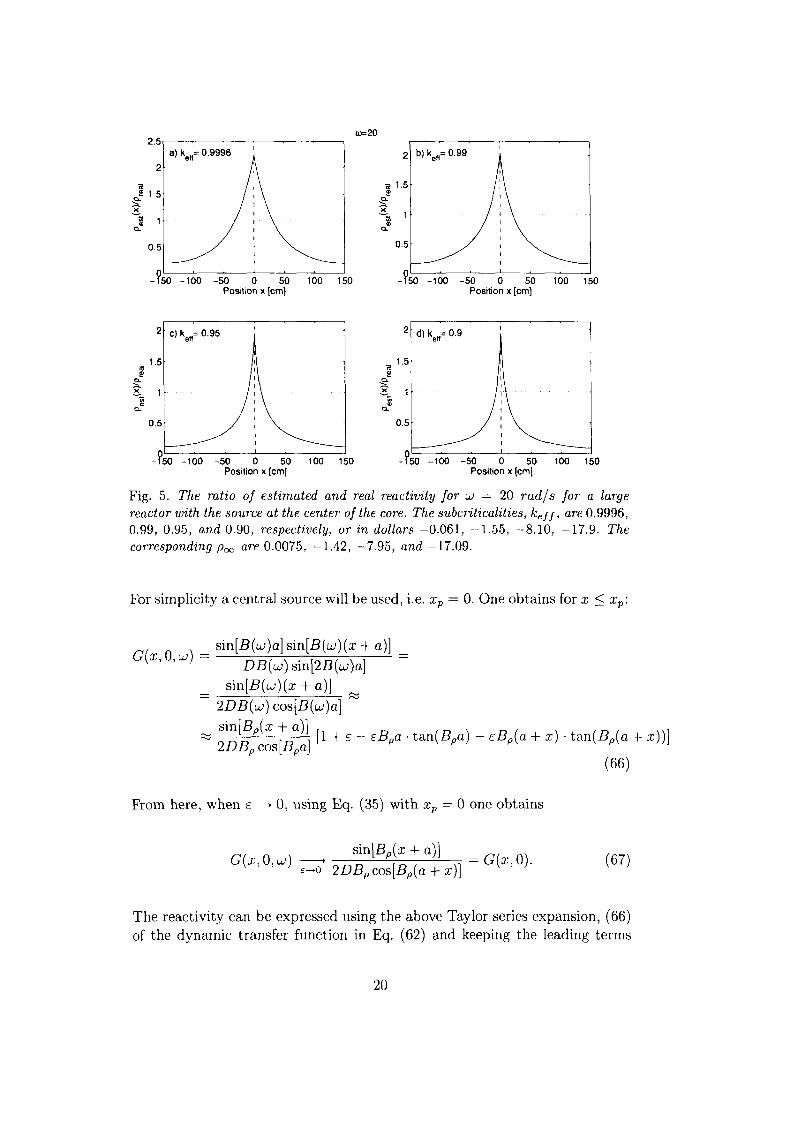
(0=20
-150 -100 -50 0 50 100 150Position x [cm]
0.5
-150 -100 -50 0 50 100 150Position x [cm]
2
1.5
2 1
0.5
0^=0.95
D150 -100 -50 0 50 100 150
Position x [cm]-150 -100 -50 0 50 100 150
Position x [cm]
Fig. 5. The ratio of estimated and real reactivity for u = 20 rad/s for a largereactor with the source at the center of the core. The subcriticalities, kejj, are 0.9996,0.99, 0.95, and 0.90, respectively, or in dollars -0.061, -1.55, -8.10, -17.9. Thecorresponding px are 0.0075, -1.42, -7.95, and-17.09.
For simplicity a central source will be used, i.e. xp = 0. One obtains for x < xp:
sin[B(u;)a] sin[B(u)(x + a)]~ DB{co)sm[2B{u})a\ ~_ sm[B(u)(x + a)]
2DB(u)cos[B{uj)a\sm[Bp(x + a)] [{ + £ _ ^ ^ ^ ^ j _ ^ ^ + x) t a n ( ^ ( f l + x))]
ZLJ\Dp COS\£JpCl\
(66)
From here, when e —* 0, using Eq. (35) with xp = 0 one obtains
G(X,0,UJ)sm\Bp{x + a))
o 2DBpcos[Bp{a += G{x,0). (67)
The reactivity can be expressed using the above Taylor series expansion, (66)of the dynamic transfer function in Eq. (62) and keeping the leading terms
20

only:
$ . = 1/e - 1 - Bpa • tan(Bpg) - Bp{a + x) cot(Bp(a + x)) ^p e s t ^ x ) - l-Bpa-t&n(Bpa)-Bp{a + x)cot(Bp(a + x)) 7Z^ °°
(68)Since, from the definition of e, one has
1 = 2e, (69)
one can write the asymptotic value of the ratio of the estimated and truereactivity in the form
^ M / ( x ) . ^ , (70)P
/ ( x ) ,
P Pwhere the function f(x) is defined as
2
~ 1 - B p [a • t a n ( B p a ) - ( a + x ) • c o t ( B p ( a + x ) ) ] ' '
For x > xp we obtain analogously:
of(x\ — (jo)
JK ' 1-Bp[a-t&n{Bpa)-{a-x)-cot{Bp(a-x))Y v '
By using expressions for p^ and p with material and geometrical constants,(70) can be put into the form
( v _
In this form the limit | p^ \—* oo and | p |—> oo can be formally enforced byletting i/Ef —* 0 which leads to
& ( 7 4 )
This shows that even if point kinetic behaviour prevails, the error of themethod is non-zero.
The investigation of the performance of the method in the alternative case ofenforcing point kinetic behaviour by letting the frequency tend to zero goeson similar lines and leads to similar results. One re-defines e as
1
then, again keeping xp = 0, one obtains for the asymptotic estimated reactiv-
21

ity, pasy, the result
0 + j.))] / W ' Ax,,
where /(x) is identical with what we obtained for f(x) in Eq. (70) for the casewhen | poo |—> oo. So similarly to Eq. (70) we arrive at
B ^ l = f[x) . ^ (76)P P
In other words, the estimated reactivity has a finite error even when the systemasymptotically approaches point kinetic behaviour with vanishing frequencies.Also, as could be expected from the asymptotic derivation, it does not matterfrom the point of view of point kinetic behaviour how the limit is reached, i.eby I P \—* oo or by u —> 0.
The above results are illustrated quantitatively for a few cases. Figures 6 and7 show the asymptotic formula, Eqs. (70)-(72) (symbols), and the generalized(non-asymptotic) formula (65) (solid lines), for UJ = 0.001 rad/s, for the smalland the large core, respectively. The two formulae agree well with each other.Except for the extreme case of a very small system with rather low frequencies,the error of the estimation is non-negligible.
5 Possible Methods for Improving the Performance
The above investigations showed that using a single neutron detector, unlessit is by chance placed to a position where the theoretical error of the methodis zero or very small, will give an error which will not disappear even in thelimit of exact point kinetic behaviour of the system. To alleviate this problem,one could resort to the fact that the original formula was derived for theamplitude factor of the factorised neutron noise, i.e. SP(u) and not for thespace-dependent noise 6<f)(x,uj). For this purpose we need to use the formula(59), i.e.
5P{LU) - 8q{u)
Recalling that<fy(z, w) = <j>p{x)5P(u) + 6xp(x, u) (77)
and the fact that 5ip(x,uj) and the critical adjoint 4>0(x) are orthogonal, theamplitude factor 6P(UJ) can be recovered from 6(j>(x,u>) as
= J 5<t>(x,u)cf>l(x)dx. (78)
22

o>=O.OO1
1
0.8
°-6
0.4
0.2
a) ka|(= 0.9996
-30 -20 -10 0 10Position x [cm]
20 30 -30 -20 -10 0 10Position x [cm]
1.5
-20 -10 0 10Position x [cm]
20 30 -20 -10 0 10Position x [cm]
20 30
Fig. 6. The ratio of estimated and real reactivity and the ratio of asymptotic andreal reactivity for u) = 0.001 rad/s and different subcriticalities, for a small reactorwith the source at the center of the core. The solid line and the line with x denotesthe estimated ratio and the asymptotic ratio, respectively.
Equation (78) suggests that instead of using the local signals, a weightedintegral, yielding the amplitude factor, could be used in the applications ofthe method. It is easy to show that there are no conceptual bugs in thisprocedure, because when using the correct SP(LO) instead of the local fluxfluctuations, there is no need for the system to behave in a point kinetic way.Hence one can apply the method also at plateau frequencies in a large system.
The feasibility of this approach can also be proven through the theory. Namely,one can use the known solutions for the noise, Eq. (42) together with (40),to construct 5P(u>) through (78), and then put it into Eq. (59) and checkthe validity of the result. After some algebra one finds the formula for theestimated reactivity which reads as
(79)m _ ~ v Jg - B2p)fG(x,xp,u)cos(B0x)dx
Pest[ ' D{Bl - B2p)fG(x, XP,LJ) cos(BQx)dx - cos(B0xp)
Using this formula we obtain for all subcriticalities that
which is exactly what is expected.
23

(i>=0.001
-?50 -100 -50 0 50Position x [cm]
100 150Position x [cm]
100 150
2
1.5
1
0.5
c)keff=0 95
150 -100 -50 0 50Position x [cm]
100 150 -150 -100 -50 0 50 100 150Position x [cm]
Fig. 7. The ratio of estimated and real reactivity and the ratio of asymptotic andreal reactivity for u> — 0.001 rad/s and different subcriticalities, for a large reactorwith the source at the center of the core. The solid line and the line with x denotesthe estimated ratio and the asymptotic ratio, respectively.
It remains to find a way of approximating the procedure of reconstructing5P(LJ) from (78). This can be done by using several detectors at differentpositions in the core, distributed relatively evenly, and then trying to ap-proximate the integral as a sum. Such an approach was used to separate thepoint kinetic and space-dependent components in other noise problems earlier(Karlsson and Pazsit, 1998). That is, one uses the approximation
5P{u>) = j 54>{x,u)4>l(x)dx (80)
Applying (80) in Eq. (79) leads to the formula of estimating the reactivityfrom a number of detector signals as
Pest{§) =
D{Bl - Bj) £, G(xu Xp, u)l - B2) Ei G{xi,xp, u) cos(B0xi)dxl - cos{B0xp)
(81)
Obviously, the quality of this approximation depends on the number of theterms used in the sum (i.e. number of detectors in the measurement), and onthe relative positioning of the detectors. It is obvious that detectors both closeto, and far away from the source, are needed to be able to eliminate the spacedependent term 8ip(x,u>) from (77) through its orthogonality with the criticaladjoint.
24

The applicability of this procedure was also investigated quantitatively. Herenow we only consider the large system, as it is the one which is interesting fromthe practical point of view. Figure 8 shows the ratio of the approximating sumand the integral as a function of number of terms in the sum the frequencyto = 20 rad/s and xp = 0, for four different subcritical values. It is seenthat the approximation converges to the value of the integral quite slowly,especially for the deeper subcriticalities.
Large reactor a=150 cm
20 40Number of terms
60 20 40Number of terms
20 40Number of terms
60 20 40Number of terms
60
Fig. 8. Approximation of the integral for ui = 20 rad/s and different subcriticalities,for a large reactor as a function of number of terms in the sum.
What is more important is how the reactivity, as estimated from Eq. (81)approximates the true reactivity. This is illustrated in Fig. 9, where the ratiois plotted as a function of number of detectors. Since the ratio is calculated forfixed detector positions, there is no explicit space dependence indicated in theresults; however it is clear that the detector positions are selected somewhatarbitrarily, and one could plot such figures for many different detector positionchoices. The results shown here can though be considered as representative.They indicate that in practice, where the number of detectors available willunlikely to exceed 10-15 for the purpose of reactivity monitoring, the methodof summing up the detector signal fluctuations does not give the expectedmeasure of improvement of the method. The situation may be even moredisadvantageous in a real case which, in contrast to the investigations herethat used a one-dimensional model, the dynamics is three-dimensional, whichamplifies the space-dependent effects further.
25

Large reactor a=150 cm1
20 40Number of detectors
60 20 40Number of detectors
20 40Number of detectors
20 40Number of detectors
60
Fig. 9. Approximation of the reactivity for to = 20 rad/s and different subcriticali-ties, for a large reactor as a function of number of detectors.
6 Conclusions
The investigation of the source modulation method of determining reactiv-ity in a source driven subcritical system led to the somewhat unexpectedconclusion that in practical applications it encounters difficulties when it isimplemented by using single detector signals to approximate the point kineticamplitude factor. The difficulty, in addition, does not lie in the large devia-tions of the behaviour of the system from point kinetics. It was shown that alarge power ADS, with the subcritical reactivities that are being consideredfor future applications, behaves in a fairly point-kinetic way. The difficultiesof the application of the method lie deeper than that; namely, just in thelimit when the system behaviour is point kinetic, the formula used becomesill-conditioned for the determination of the reactivity. In other words, even inthe case of rather good point kinetic behaviour of the system, the error of thereactivity formula is still significant. Even methods of using several detectors,which in other cases were helpful in order to separate the point kinetic com-ponent from the total noise, perform poorly in this case. Hence, most likely,the source modulation method, as well as related methods such as the protonimportance method, only can be used in a relative way, after having beencalibrated by other methods.
26

7 Acknowledgement
This work was financially supported by the Swedish Centre for Nuclear Tech-nology (SKC) and the Swedish Nuclear Power Inspectorate (SKI).
References
Cacuci, D., 2004. On the neutron kinetics and control of accelerator-drivensystems. Nuclear Science and Engineering 148, 55-66.
Carta, M., D'Angelo, A., 1999. Subcriticality-level evaluation in accelerator-driven systems by harmonic modulation of the external source. NuclearScience and Engineering 133, 282-292.
Dulla, S., Ravetto, P., Rostagno, M., 2004. Transport effects for source-oscillated problems in subcritical systems. Nuclear Science and Engineering148, 89-102.
Dulla, S., Ravetto, P., Rostagno, M., Bianchini, G., Carta, M., D'Angelo, A.,2005. Some features of spatial neutron kinetics for multiplying systems.Nuclear Science and Engineering 149, 88-100.
Eriksson, B. M., Cahalan, J. E., Yang, W. S., 2005. On the performance ofpoint kinetics for the analysis of accelerator-driven systems. Nuclear Scienceand Engineering 149, 298-311.
Garis, N., Pazsit, I., Sandhi, D., 1996. Modelling of a vibrating reactor bound-ary and calculation of the induced neutron noise. Annals of Nuclear Energy23, 1197-1208.
Imel, G., Naberejnev, D., Palmiotti, G., Philibert, H., Granget, G., Mandard,L., Soule, R., Fougeras, P., Steckmeyer, J., Lecolley, F. R., Carta, M., Rosa,R., Grossi, A., S.Monti, Peluso, V., Sarotto, M., 2004. The trade sourcemultiplication experiments. In: Proc. PHYSOR 2004 - The Physics of FuelCycles and Advanced Nuclear Systems: Global Developments. Chicago, Illi-nois, April 25-29, 2004.
Karlsson, J., Pazsit, I., 1998. Noise decomposition in bwrs with applicationsto stability monitoring. Nuclear Science and Engineering 128, 225-242.
Pazsit, I., 2003. Kinetic approximations and noise theory in source-drivensubcritical systems. In: Proc. Nuclear Mathematical and ComputationalSciences: A Century in Review, A Century Anew. Gatlinburg, Tenessee,April 6-11, 2003.
Pazsit, I., Arzhanov, V., 1999. Theory of neutron noise induced by source fluc-tuations in accelerator-driven subcritical reactors. Annals of Nuclear Energy26, 1371-1393.
Ravetto, P., Rostagno, M., Bianchini, G., Carta, M., D'Angelo, A., 2004. Ap-plication of the multipoint method to the kinetics of accelerator-driven sys-tems. Nuclear Science and Engineering 148, 79-88.
27

Rubbia, C, Carta, M., Burgio, N., Ciavola, C, D'Angelo, A., Dodaro, A.,Festinesi, A., Monti, S., Santagata, A., Troiani, F., Salvatores, M., Delpech,M., Kadi, Y., Buono, S., Ferrari, A., Herrera, A., Martinez, Zanini, L., Imel,G., 2004. Neutronic analyses of the trade demonstration facility. NuclearScience and Engineering 148, 103-123.
Sjostrand, N., 1959. On the theory underlying diffusion measurements withpulsed neutron sources. Arkiv for Fysik 15, 147-158.
Soule, FL, Assal, W., Chaussonnet, P., Destouches, C, Domergue, C, Jammes,C, Lebrat, J.-F., Mellier, F., Perret, G., Rimpault, G., Serviere, H., Imel,G., Thomas, G., Villamarin, D., Gonzalez-Romero, E., Plaschy, M., Chawla,R., Kloosterman, J., Rugama, Y., Billebaud, A., Brissot, R., Heuer, D.,Kerveno, M., Brun, C. L., Loiseaux, J.-M., Meplan, O., Merle, E., Perdu,F., Vollaire, J., Baeten, P., 2004. Neutronic studies in support of ads: Themuse experiments in the masurca facility. Nuclear Science and Engineering148, 124-152.
Takahashi, H., An, Y., Chen, X., 1998. Transactions of American NuclearSociety 78, 282.
28


