Ch 07 Solutions Fluid Mechanics (White, 5th)
87
Chapter 7 • Flow Past Immersed Bodies 7.1 For flow at 20 m/s past a thin flat plate, estimate the distances x from the leading edge at which the boundary layer thickness will be either 1 mm or 10 cm, for (a) air; and (b) water at 20°C and 1 atm. Solution: (a) For air, take ρ = 1.2 kg/m 3 and µ = 1.8E−5 kg/m⋅s. Guess laminar flow: 2 2 1/2 5.0 (0.001) (1.2)(20) , : ( —1 ) 25 25(1.8 5) laminar x U or x Ans. air mm x E Re δ δρ µ = = = = − 0.0533 m 1.2(20)(0.0533)/1.8 5 71,000 , x Check Re E OK laminar flow = −= (a) For the thicker boundary layer, guess turbulent flow: 1/7 0.16 , (a—10 ) ( /) turb solve for Ans. cm x Ux δ ρ µ = x 6.06 m = 8.1 6, , x Check Re E OK turbulent flow = (b) For water, take ρ = 998 kg/m 3 and µ = 0.001 kg/m⋅s. Both cases are probably turbulent: δ = 1 mm: x turb = 0.0442 m, Re x = 882,000 (barely turbulent) Ans. (water—1 mm) δ = 10 cm: x turb = 9.5 m, Re x = 1.9E8 (OK, turbulent) Ans. (water—10 cm) 7.2 Air, equivalent to a Standard Altitude of 4000 m, flows at 450 mi/h past a wing which has a thickness of 18 cm, a chord length of 1.5 m, and a wingspan of 12 m. What is the appropriate value of the Reynolds number for correlating the lift and drag of this wing? Explain your selection. Solution: Convert 450 mi/h = 201 m/s, at 4000 m, ρ = 0.819 kg/m⋅s, T = 262 K, µ = 1.66E−5 kg/m⋅s. The appropriate length is the chord, C = 1.5 m, and the best parameter to correlate with lift and drag is Re C = (0.819)(201)(1.5)/1.66E−5 = 1.5E7 Ans. 7.3 Equation (7.1b) assumes that the boundary layer on the plate is turbulent from the leading edge onward. Devise a scheme for determining the boundary-layer thickness more accurately when the flow is laminar up to a point Re x,crit and turbulent thereafter. Apply this scheme to computation of the boundary-layer thickness at x = 1.5 m in 40 m/s
-
Upload
stutsmagee5888 -
Category
Documents
-
view
7.470 -
download
141
Transcript of Ch 07 Solutions Fluid Mechanics (White, 5th)

Chapter 7 • Flow Past Immersed Bodies
7.1 For flow at 20 m/s past a thin flat plate, estimate the distances x from the leading edge at which the boundary layer thickness will be either 1 mm or 10 cm, for (a) air; and (b) water at 20°C and 1 atm.
Solution: (a) For air, take ρ = 1.2 kg/m3 and µ = 1.8E−5 kg/m⋅s. Guess laminar flow:
2 2
1/2
5.0 (0.001) (1.2)(20), : ( —1 )
25 25(1.8 5)laminar
x
Uor x Ans. air mm
x ERe
δ δ ρµ
= = = =−
0.0533 m
1.2(20)(0.0533)/1.8 5 71,000 , xCheck Re E OK laminar flow= − =
(a) For the thicker boundary layer, guess turbulent flow:
1/7
0.16, (a—10 )
( / )turb solve for Ans. cmx Ux
δρ µ
= x 6.06 m=
8.1 6, , xCheck Re E OK turbulent flow=
(b) For water, take ρ = 998 kg/m3 and µ = 0.001 kg/m⋅s. Both cases are probably turbulent:
δ = 1 mm: xturb = 0.0442 m, Rex = 882,000 (barely turbulent) Ans. (water—1 mm)
δ = 10 cm: xturb = 9.5 m, Rex = 1.9E8 (OK, turbulent) Ans. (water—10 cm)
7.2 Air, equivalent to a Standard Altitude of 4000 m, flows at 450 mi/h past a wing which has a thickness of 18 cm, a chord length of 1.5 m, and a wingspan of 12 m. What is the appropriate value of the Reynolds number for correlating the lift and drag of this wing? Explain your selection.
Solution: Convert 450 mi/h = 201 m/s, at 4000 m, ρ = 0.819 kg/m⋅s, T = 262 K, µ = 1.66E−5 kg/m⋅s. The appropriate length is the chord, C = 1.5 m, and the best parameter to correlate with lift and drag is ReC = (0.819)(201)(1.5)/1.66E−5 = 1.5E7 Ans.
7.3 Equation (7.1b) assumes that the boundary layer on the plate is turbulent from the leading edge onward. Devise a scheme for determining the boundary-layer thickness more accurately when the flow is laminar up to a point Rex,crit and turbulent thereafter. Apply this scheme to computation of the boundary-layer thickness at x = 1.5 m in 40 m/s

476 Solutions Manual • Fluid Mechanics, Fifth Edition
flow of air at 20°C and 1 atm past a flat plate. Compare your result with Eq. (7.1b). Assume Rex,crit ≈ 1.2E6.
Fig. P7.3
Solution: Given the transition point xcrit, Recrit, calculate the laminar boundary layer thick-ness δc at that point, as shown above, δc/xc ≈ 5.0/Recrit
1/2. Then find the “apparent” distance upstream, Lc, which gives the same turbulent boundary layer thickness,
c
1/7c c L/L 0.16/Re .δ ≈
Then begin xeffective at this “apparent origin” and calculate the remainder of the turbulent boundary layer as δ/xeff ≈ 0.16/Reeff
1/7. Illustrate with a numerical example as requested. For air at 20°C, take ρ = 1.2 kg/m3 and µ = 1.8E−5 kg/m⋅s.
ccrit c c 1/2
1/6 1/67/6 7/6c
c
1.2(40)x 5.0(0.45)Re 1.2E6 if x 0.45 m, then 0.00205 m
1.8E 5 (1.2E6)
U 0.00205 1.2(40)Compute L 0.0731 m
0.16 0.16 1.8E 5
δ
δ ρµ
= = = = ≈−
= = ≈ −
Finally, at x = 1.5 m, compute the effective distance and the effective Reynolds number:
eff c c eff
eff 1.5 m 1/7 1/7eff
1.2(40)(1.123)x x L x 1.5 0.0731 0.45 1.123 m, Re 2.995E6
1.8E 50.16x 0.16(1.123)
Re (2.995E6)Ans.δ
= + − = + − = = ≈−
≈ = ≈| 0.0213 m
Compare with a straight all-turbulent-flow calculation from Eq. (7.1b):
x 1.5 m 1/7
1.2(40)(1.5) 0.16(1.5)Re 4.0E6, whence (25% higher) .
1.8E 5 (4.0E6)Ansδ= ≈ ≈ ≈
−| 0.027 m
7.4 A smooth ceramic sphere (SG = 2.6) is immersed in a flow of water at 20°C and 25 cm/s. What is the sphere diameter if it is encountering (a) creeping motion, Red = 1; or (b) transition to turbulence, Red = 250,000?

Chapter 7 • Flow Past Immersed Bodies 477
Solution: For water, take ρ = 998 kg/m3 and µ = 0.001 kg/m⋅s. (a) Set Red equal to 1:
3(998 kg/m )(0.25 m/s)Re 1
0.001 kg/m s
Solve for 4 m (a)
dVd d
Ans.
ρµ
µ
= = =⋅
=d 4E 6 m= −
(b) Similarly, at the transition Reynolds number,
3(998 kg/m )(0.25 m/s)Re 250000 , solve for (b)
0.001 kg/m sdd
Ans.= =⋅
d 1.0 m=
7.5 SAE 30 oil at 20°C flows at 1.8 ft3/s from a reservoir into a 6-in-diameter pipe. Use flat-plate theory to estimate the position x where the pipe-wall boundary layers meet in the center. Compare with Eq. (6.5), and give some explanations for the discrepancy.
Solution: For SAE 30 oil at 20°C, take ρ = 1.73 slug/ft3 and µ = 0.00607 slug/ft⋅s. The average velocity and pipe Reynolds number are:
avg D2
Q 1.8 ft VD 1.73(9.17)(6/12)V 9.17 , Re 1310 (laminar)
A s 0.00607( /4)(6/12)
ρµπ
= = = = = =
Using Eq. (7.1a) for laminar flow, find “xe” where δ = D/2 = 3 inches:
2 2
eV (3/12) (1.73)(9.17)
x (flat-plate boundary layer estimate)25 25(0.00607)
Ans.δ ρ
µ≈ = ≈ 6.55 ft
This is far from the truth, much too short. Equation (6.5) for laminar pipe flow predicts
e Dx 0.06D Re 0.06(6/12 ft)(1310) Alternate Ans.= = ≈ 39 ft
The entrance flow is accelerating, as the core velocity increases from V to 2V, and the accelerating boundary layer is much thinner and takes much longer to grow to the center. Ans.
7.6 For the laminar parabolic boundary-layer profile of Eq. (7.6), compute the shape factor “H” and compare with the exact Blasius-theory result, Eq. (7.31).

478 Solutions Manual • Fluid Mechanics, Fifth Edition
Solution: Given the profile approximation u/U ≈ 2η − η2, where η = y/δ, compute 1
2 2
0 0
12
0 0
u u 21 dy (2 )(1 2 )d
U U 15
u 1* 1 dy (1 2 ) d
U 3
δ
δ
θ δ η η η η η δ
δ δ η η η δ
= − = − − + =
= − = − + =
Hence H = δ ∗/θ = (δ/3)/(2δ/15) ≈ 2.5 (compared to 2.59 for Blasius solution)
7.7 Air at 20°C and 1 atm enters a 40-cm-square duct as in Fig. P7.7. Using the “displacement thickness” concept of Fig. 7.4, estimate (a) the mean velocity and (b) the mean pressure in the core of the flow at the position x = 3 m. (c) What is the average gradient, in Pa/m, in this section?
Fig. P7.7
Solution: For air at 20°C, take ρ = 1.2 kg/m3 and µ = 1.8E−5 kg/m⋅s. Using laminar boundary-layer theory, compute the displacement thickness at x = 3 m:
x 1/2 1/2x
Ux 1.2(2)(3) 1.721x 1.721(3)Re 4E5 (laminar), * 0.0082 m
1.8E 5 Re (4E5)
ρ δµ
= = = = = ≈−
2 2o
exito
L 0.4Then, by continuity, V V (2.0)
*L 2 0.4 0.0164
(a)Ans.
δ = = − −
≈ m2.175
s
The pressure change in the (frictionless) core flow is estimated from Bernoulli’s equation:
2 2 2 2exit exit o o exit
1.2 1.2p V p V , or: p (2.175) 1 atm (2.0)
2 2 2 2
ρ ρ+ = + + = +
x 3mSolve for p 1 atm 0.44 Pa (b)Ans.= = − =| 0.56 Pa
The average pressure gradient is ∆p/x = (−0.44/3.0) ≈ −0.15 Pa/m Ans. (c)

Chapter 7 • Flow Past Immersed Bodies 479
7.8 Air, ρ =1.2 kg/m3 and µ = 1.8E−5 kg/m⋅s, flows at 10 m/s past a flat plate. At the trailing edge of the plate, the following velocity profile data are measured: y, mm: 0 0.5 1.0 2.0 3.0 4.0 5.0 6.0
u, m/s: 0 1.75 3.47 6.58 8.70 9.68 10.0 10.0
u(U − u), m2/s: 0 14.44 22.66 22.50 11.31 3.10 0.0 0.0 If the upper surface has an area of 0.6 m2, estimate, using momentum concepts, the friction drag, in newtons, on the upper surface.
Solution: Make a numerical estimate of drag from Eq. (7.2): F = ρb u(U − u)dy. We have added the numerical values of u(U − u) to the data above. Using the trapezoidal rule between each pair of points in this table yields
3
0
1 0 14.44 14.44 22.66 m( ) 0.5 0.061
1000 2 2 su U u dy
δ + + − ≈ + + ≈
The drag is approximately F = 1.2b(0.061) = 0.073b newtons or 0.073 N/m. Ans.
7.9 Repeat the flat-plate momentum analysis of Sec. 7.2 by replacing the parabolic profile, Eq. (7.6), with the more accurate sinusoidal profile:
sin2
u y
U
πδ
≈
Compute momentum-integral estimates of Cf, δ/x, δ ∗/x, and H.
Solution: Carry out the same integrations as Section 7.2, but results are more accurate:
0 0
u u 4 u 21 dy 0.1366 ; * 1 dy 0.3634
U U 2 U
δ δπ πθ δ δ δ δ δπ π− − = − ≈ = = − ≈ =
2w
x x
2 )U d 4 4.80U , integrate to: (5% low)
2 dx 2 x Re Re
/π ππ π δτ µ ρ δδ π
(4 −− ≈ = ≈ ≈
Substitute these results back to obtain the desired (accurate) dimensionless expressions:
f* *
; C ; ; H (a, b, c, d)x x x
Ans.δ θ δ δ
θ≈ = ≈ ≈ = ≈
x x x
4.80 0.655 1.7432.66
Re Re Re

480 Solutions Manual • Fluid Mechanics, Fifth Edition
7.10 Repeat Prob. 7.9, using the polynomial profile suggested by K. Pohlhausen in 1921: 3 4
3 42 2
u y y y
U δ δ δ≈ − +
Does this profile satisfy the boundary conditions of laminar flat-plate flow?
Solution: Pohlhausen’s quadratic profile satisfies no-slip at the wall, a smooth merge with u → U as y → δ, and, further, the boundary-layer curvature condition at the wall. From Eq. (7.19b),
wall
2 2
wall2 2
u u u u pu v 0, or: 0 for flat-plate flow 0
x y xy y
∂ ∂ µ ∂ ∂ ∂∂ ∂ ρ ∂∂ ∂
+ − = = = |
This profile gives the following integral approximations:
2w
37 3 2U d 37; * ; U
315 10 dx 315θ δ δ δ τ µ ρ δ
δ ≈ ≈ ≈ ≈
, integrate to obtain:
fx
(1260/37); C ;
x xRe
*; H (a, b, c, d)
xAns.
δ θ
δ
≈ ≈ = ≈
≈ ≈
x x
x
5.83 0.685
Re Re
1.7512.554
Re
7.11 Air at 20°C and 1 atm flows at 2 m/s past a sharp flat plate. Assuming that the Kármán parabolic-profile analysis, Eqs. (7.6−7.10), is accurate, estimate (a) the local velocity u; and (b) the local shear stress τ at the position (x, y) = (50 cm, 5 mm).
Solution: For air, take ρ = 1.2 kg/m3 and µ = 1.8E−5 kg/m⋅s. First compute Rex and δ(x): The location we want is y/δ = 5 mm/10.65 mm = 0.47, and Eq. (7.6) predicts local velocity:
22
2
2(0.5 m, 5 mm) (2 m/s)[2(0.47) (0.47) ] (a)
y yu U Ans.
δ δ
≈ − = − = 1.44 m/s
The local shear stress at this y position is estimated by differentiating Eq. (7.6):
2 (1.8 5 kg/m s)(2 m/s)(0.5 m, 5 mm) 2 [2 2(0.47)]
0.01065 m
(b)
u U y E
y
Ans.
∂ µτ µ∂ δ δ
− ⋅ = ≈ − = −
= 0.0036 Pa

Chapter 7 • Flow Past Immersed Bodies 481
7.12 The velocity profile shape u/U ≈ 1 − exp(−4.605y/δ ) is a smooth curve with u = 0 at y = 0 and u = 0.99U at y = δ and thus would seem to be a reasonable substitute for the parabolic flat-plate profile of Eq. (7.3). Yet when this new profile is used in the integral analysis of Sec. 7.3, we get the lousy result 1/2/ 9.2/Rexxδ ≈ , which is 80 percent high. What is the reason for the inaccuracy? [Hint: The answer lies in evaluating the laminar boundary-layer momentum equation (7.19b) at the wall, y = 0.]
Solution: This profile satisfies no-slip at the wall and merges very smoothly with u → U at the outer edge, but it does not have the right shape for flat-plate flow. It does not satisfy the zero curvature condition at the wall (see Prob. 7.10 for further details):
∂δ∂ δ=
≈ − ≈ − ≠
|22
y 02 2
u 4.605 21.2UEvaluate U 0 by a long measure!
y
The profile has a strong negative curvature at the wall and simulates a favorable pressure gradient shape. Its momentum and displacement thickness are much too small.
7.13 Derive modified forms of the laminar boundary-layer equations for flow along the outside of a circular cylinder of constant R, as in Fig. P7.13. Consider the two cases (a) R;δ and (b) δ ≈ R. What are the boundary conditions?
Solution: The Navier-Stokes equations for cylindrical coordinates are given in Appendix D, with “x” in the Fig. P7.13 denoting the axial coordinate “z.” Assume “axisymmetric” flow, that is, vθ = 0 and ∂/∂θ = 0 everywhere. The boundary layer assumptions are:
Fig. P7.13
r rr
u u v vv u; ; ;
x r x r
∂ ∂ ∂ ∂∂ ∂ ∂ ∂
hence r-momentum (Eq. D-5) becomes p
0r
≈∂∂
Thus p ≈ p(x) only, and for a long straight cylinder, p ≈ constant and U ≈ constant
Then, with ∂ p /∂ x = 0, the x-momentum equation (D-7 in the Appendix) becomes
when R (b)Ans.δ ≈
∂ ∂ µ ∂ ∂ρ ρ∂ ∂ ∂ ∂r
u u uu v r
x r r r r+ ≈
482 Solutions Manual • Fluid Mechanics, Fifth Edition
plus continuity: when R (b)Ans.δ ≈∂ ∂∂ ∂ r
u 1(rv ) 0
x r r+ ≈
For thick boundary layers (part b) the radial geometry is important.
If, however, the boundary layer is very thin, R,δ then r = R + y ≈ R itself, and we can use (x, y):
Continuity: if R (a)Ans.δ ∂ ∂∂ ∂
ru v0
x y+ ≈
x-momentum: if R . (a)Ansδ ∂ ∂ ∂ρ ρ µ∂ ∂ ∂
2
r 2
u u uu v
x y y+ ≈
Thus a thin boundary-layer on a cylinder is exactly the same as flat-plate (Blasius) flow.
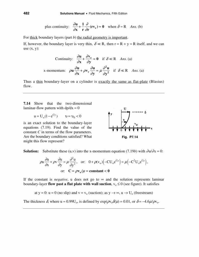
7.14 Show that the two-dimensional laminar-flow pattern with dp/dx = 0
Cyo 0u U (1 e ) 0= − υ = υ <
is an exact solution to the boundary-layer equations (7.19). Find the value of the constant C in terms of the flow parameters. Are the boundary conditions satisfied? What might this flow represent?
Fig. P7.14
Solution: Substitute these (u,v) into the x-momentum equation (7.19b) with ∂ u/∂ x = 0:
( ) ( )2
Cy 2 Cyo o o2
u u uu v , or: 0 (v ) CU e C U e ,
x y y
or: /
∂ ∂ ∂ρ ρ µ ρ µ∂ ∂ ∂
+ ≈ + − ≈ −
oC v constant 0= = <ρ µ
If the constant is negative, u does not go to ∞ and the solution represents laminar boundary-layer flow past a flat plate with wall suction, vo ≤ 0 (see figure). It satisfies
at y = 0: u = 0 (no slip) and v = vo (suction); as y → ∞, u → Uo (freestream)
The thickness δ, where u ≈ 0.99Uo, is defined by exp(ρvoδ/µ) = 0.01, or δ = −4.6µ/ρvo.
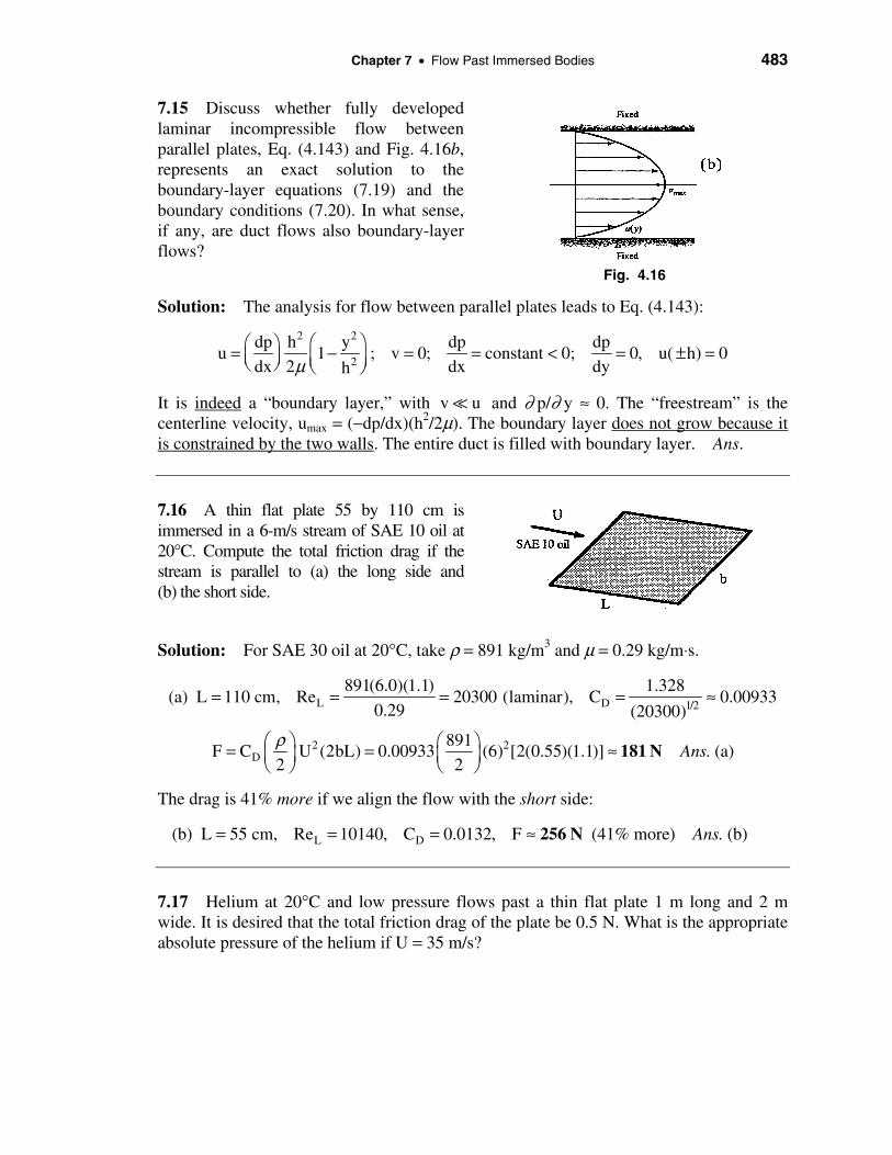
Chapter 7 • Flow Past Immersed Bodies 483 7.15 Discuss whether fully developed laminar incompressible flow between parallel plates, Eq. (4.143) and Fig. 4.16b, represents an exact solution to the boundary-layer equations (7.19) and the boundary conditions (7.20). In what sense, if any, are duct flows also boundary-layer flows?
Fig. 4.16
Solution: The analysis for flow between parallel plates leads to Eq. (4.143):
2 2
2
dp h y dp dpu 1 ; v 0; constant 0; 0, u( h) 0
dx 2 dx dyhµ = − = = < = ± =
It is indeed a “boundary layer,” with v u and ∂ p/∂ y ≈ 0. The “freestream” is the centerline velocity, umax = (−dp/dx)(h2/2µ). The boundary layer does not grow because it is constrained by the two walls. The entire duct is filled with boundary layer. Ans.
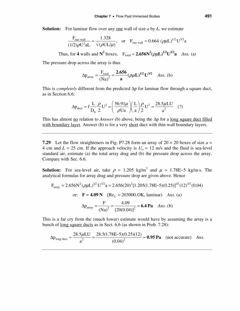
7.16 A thin flat plate 55 by 110 cm is immersed in a 6-m/s stream of SAE 10 oil at 20°C. Compute the total friction drag if the stream is parallel to (a) the long side and (b) the short side.
Solution: For SAE 30 oil at 20°C, take ρ = 891 kg/m3 and µ = 0.29 kg/m⋅s.
L D 1/2
891(6.0)(1.1) 1.328(a) L 110 cm, Re 20300 (laminar), C 0.00933
0.29 (20300)= = = = ≈
2 2D
891F C U (2bL) 0.00933 (6) [2(0.55)(1.1)] (a)
2 2Ans.
ρ = = ≈
181 N
The drag is 41% more if we align the flow with the short side:
L D(b) L 55 cm, Re 10140, C 0.0132, F (41% more) (b)Ans.= = = ≈ 256 N
7.17 Helium at 20°C and low pressure flows past a thin flat plate 1 m long and 2 m wide. It is desired that the total friction drag of the plate be 0.5 N. What is the appropriate absolute pressure of the helium if U = 35 m/s?

484 Solutions Manual • Fluid Mechanics, Fifth Edition
Solution: For helium at 20°C, take R = 2077 J/kg⋅K and µ = 1.97E−5 kg/m⋅s. It is best to untangle the dimensionless drag coefficient relation to reveal the (unknown) density:
1/22 2 1/2 3/2
D 1/2
1/2 3/2 3
1.328F C U 2bL U (2bL) 1.328b( L) U ,
2 2( UL)
or: 0.5 N 1.328(2.0)[ (1.97E 5)(1.0)] (35) , solve for 0.0420 kg/m
p RT (0.042)(2077)(293) Ans.
ρ µ ρ ρµρ
ρ ρ
ρ
= = =
= − ≈
∴ = = ≈ 25500 Pa
Check ReL = ρUL/µ ≈ 75000, OK, laminar flow.
7.18 The approximate answers to Prob. 7.11 are u ≈ 1.44 m/s and τ ≈ 0.0036 Pa at x = 50 cm and y = 5 mm. [Do not reveal this to your friends who are working on Prob. 7.11.] Repeat that problem by using the exact Blasius flat-plate boundary-layer solution.
Solution: (a) Calculate the Blasius variable η (Eq. 7.21), then find f ′ = u/U at that position:
2
2 m/s(0.005 m) 2.58,
(0.000015 m /s)(0.5 m)
0.768, (a)
Uy
x
uTable 7.1: u Ans.
U
ην
= = =
≈ ∴ ≈ 1.54 m/s
(b) Differentiate Eq. (7.21) to find the local shear stress:
[ ( )] ( ). At 2.58, estimate ( ) 0.217u U
Uf U f fy y x
∂ ∂τ µ µ η µ η η η∂ ∂ ν
= = = = ≈′ ′′ ′′
(2.0)Then (0.000018)(2.0) (0.217) (b)
(0.000015)(0.5)Ans.τ ≈ ≈ 0.0040 Pa
7.19 Program a method of numerical solution of the Blasius flat-plate relation, Eq. (7.22), subject to the conditions in (7.23). You will find that you cannot get started without knowing the initial second derivative f″(0), which lies between 0.2 and 0.5. Devise an iteration scheme which starts at f″(0) ≈ 0.2 and converges to the correct value. Print out u/U = f ′(η) and compare with Table 7.1.
Solution: This is a good exercise for students who are familiar with some integration scheme, such as Runge-Kutta, or have some built-in software, such as MathCAD. The solutions are very well behaved, that is, no matter what the guess for 0.2 < f″(0) < 0.5, the value of f ′(η) approaches a constant value as η → ∞. The student can then easily

Chapter 7 • Flow Past Immersed Bodies 485
interpolate to the correct value f″(0) ≈ 0.33206. One detail is that “∞” must be chosen and occurs at about η ≈ 10.
7.20 Air at 20°C and 1 atm flows at 20 m/s past the flat plate in Fig. P7.20. A pitot stagnation tube, placed 2 mm from the wall, develops a manometer head h = 16 mm of Meriam red oil, SG = 0.827. Use this information to estimate the downstream position x of the pitot tube. Assume laminar flow.
Fig. P7.20
Solution: For air at 20°C, take ρ = 1.2 kg/m3 and µ = 1.8E−5 kg/m⋅s. Assume constant stream pressure, then the manometer can be used to estimate the local velocity u at the position of the pitot inlet:
mano o oil air manop p p ( )gh [0.827(998) 1.2](9.81)(0.016) 129 Paρ ρ∞∆ = − = − = − ≈ 1/2 1/2
pitot inletThen u [2 p/ ] [2(129)/1.2] 14.7 m/sρ≈ ∆ = ≈
Now, with u known, the Blasius solution uses u/U to determine the position η:
1/2
2 2
u 14.70.734, Table 7.1 read 2.42 y(U/ x)
U 20
or: x (U/ )(y/ ) (20/1.5E 5)(0.002/2.42) Ans.
η ν
ν η
= = ≈ =
−= = ≈ 0.908 m
Check ReX = (20)(0.908)/(1.5E−5) ≈ 1.21E6, OK, laminar if the flow is very smooth.
7.21 For the experimental set-up of Fig. P7.20, suppose the stream velocity is unknown and the pitot stagnation tube is traversed across the boundary layer of air at 1 atm and 20°C. The manometer fluid is Meriam red oil, and the following readings are made:
y, mm: 0.5 1.0 1.5 2.0 2.5 3.0 3.5 4.0 4.5 5.0
h, mm: 1.2 4.6 9.8 15.8 21.2 25.3 27.8 29.0 29.7 29.7
Using this data only (not the Blasius theory) estimate (a) the stream velocity, (b) the boundary layer thickness, (c) the wall shear stress, and (d) the total friction drag between the leading edge and the position of the pitot tube.

486 Solutions Manual • Fluid Mechanics, Fifth Edition
Solution: As in Prob. 7.20, the air velocity u = [2(ρoil − ρair)gh/ρair]1/2. For the oil, take
ρoil = 0.827(998) = 825 kg/m3. For air, ρ = 1.2 kg/m3 and µ = 1.8E−5 kg/m⋅s. (a, b) We see that h levels out to 29.7 mm at y = 4.5 mm. Thus
1/2U [2(825 1.2)(9.81)(0.0297)/1.2] (a) (b)Ans. Ans.δ∞ = − = =20.0 m/s 4.5 mm
(c) The wall shear stress is estimated from the derivative of velocity at the wall:
04.02 0
(1.8 5) (c)0.0005 0w y
u uE Ans.
y y
∂τ µ µ∂ =
∆ − = ≈ ≈ − ≈ ∆ −| 0.14 Pa
where we have calculated unear-wall = [2(825 − 1.2)(9.81)(0.0012)/1.2]1/2 = 4.02 m/s. (d) To estimate drag, first see if the boundary layer is laminar. Evaluate Reδ :
,1.2(20)(0.0045)
6000, which implies 1.44 61.8 5 x laminar
URe Re E
Eδρ δ
µ= = ≈ ≈
−
This is a little high, maybe, but let us assume a smooth wall, therefore laminar, in which case the drag is twice the local shear stress times the wall area. From Prob. 7.20, we estimated the distance x to be 0.908 m. Thus
w2 2(0.14 Pa)(0.908 m)(1.0) per meter of width. (d)xb Ans.τ≈ = ≈F 0.25 N
7.22 For the Blasius flat-plate problem, Eqs. (7.21) to (7.23), does a two-dimensional stream function ψ(x, y) exist? If so, determine the correct dimensionless form for ψ, assuming that ψ = 0 at the wall, y = 0.
Solution: A stream function ψ(x, y) does exist because the flow satisfies the two-dimensional equation of continuity, Eq. (7.19a). That is, u = ∂ ψ/∂ y and v = −∂ ψ/∂ x. Given the “Blasius” form of u, we may integrate to find ψ :
( )y
x const0 0
df dfu , thus u dy U dy U d x/U
y d d
η∂ψ ψ η ν∂ η η=
= = = = |
1/2 /
0
or ( xU) df Ans.η
ψ ν= =1 2xU) f(ν
The integration assumes that ψ = 0 at y = 0, which is very convenient.

Chapter 7 • Flow Past Immersed Bodies 487 7.23 Suppose you buy a 4 × 8-ft sheet of plywood and put it on your roof rack, as in the figure. You drive home at 35 mi/h. (a) If the board is perfectly aligned with the airflow, how thick is the boundary layer at the end? (b) Estimate the drag if the flow remains laminar. (c) Estimate the drag for (smooth) turbulent flow.
Fig. P7.23
Solution: For air take ρ = 1.2 kg/m3 and µ = 1.8E−5 kg/m⋅s. Convert L = 8 ft = 2.44 m and U = 35 mi/h = 15.6 m/s. Evaluate the Reynolds number, is it laminar or turbulent?
1.2(15.6)(2.44)Re 2.55 6
1.8 5LUL
E probably laminar turbulentE
ρµ
= = = +−
(a) Evaluate the range of boundary-layer thickness between laminar and turbulent:
5.0
: 0.00313, : 0.00765 2.44 2.55 6
Laminar or mL m E
δ δ δ= ≈ = ≈ = 0.30 in
1/7
0.16: 0.0195, : 0.047 (a)
2.44 (2.55 6)Turbulent or m Ans.
E
δ δ≈ = ≈ = 1.9 in
(b, c) Evaluate the range of boundary-layer drag for both laminar and turbulent flow. Note that, for flow over both sides, the appropriate area A = 2bL:
2 21.328 1.2(15.6) (2.44 1.22 2 ) (b)
2 22.55 6lam DF C U A sides Ans.
E
ρ = ≈ × × = 0.73 N
21/7
0.031 1.2(15.6) (2.44 1.22 2 ) (c)
2(2.55 6)turbF sides Ans.
E
≈ × × =
3.3 N
We see that the turbulent drag is about 4 times larger than laminar drag.
7.24 Air at 20°C and 1 atm flows past the flat plate in Fig. P7.24. The two pitot tubes are each 2 mm from the wall. The manometer fluid is water at 20°C. If U = 15 m/s and L = 50 cm, determine the values of the manometer readings h1 and h2 in cm. Assume laminar boundary-layer flow.

488 Solutions Manual • Fluid Mechanics, Fifth Edition
Fig. P7.24
Solution: For air at 20°C, take ρ = 1.2 kg/m3 and µ = 1.8E−5 kg/m⋅s. The velocities u at each pitot inlet can be estimated from the Blasius solution:
1/2 1/21 1
1
(1) y[U/ x ] (0.002)15/[1.5E 5(0.5)] 2.83, Table 7.1: read f 0.816
Then u Uf 15(0.816) 12.25 m/s
η ν= = − = ≈′= = ≈′
1/22 2 2(2) y[U/vx ] 2.0, f 0.630, u 15(0.630) 9.45 m/sη = = ≈ = ≈′
Assume constant stream pressure, then the manometers are a measure of the local velocity u at each position of the pitot inlet, so we can find ∆p across each manometer:
2 21 1 1 1
1.2p u (12.25) 90 Pa gh (998 1.2)(9.81)h ,
2 2
ρ ρ∆ = = = = ∆ = − 1h 9.2 mm≈
2 22 2 2
1.2p u (9.45) 54 Pa (998 1.2)(9.81)h , or:
2 2Ans.
ρ∆ = = = = − 2h 5.5 mm≈
7.25 Consider the smooth square 10 by 10 cm duct in Fig. P7.25. The fluid is air at 20°C and 1 atm, flowing at Vavg = 24 m/s. It is desired to increase the pressure drop over the 1-m length by adding sharp 8-mm-long flat plates across the duct, as shown. (a) Estimate the pressure drop if there are no plates. (b) Estimate how many plates are needed to generate an additional 100 Pa of pressure drop.
Fig. P7.25

Chapter 7 • Flow Past Immersed Bodies 489
Solution: For air, take ρ = 1.2 kg/m3 and µ = 1.8E−5 kg/m⋅s. (a) Compute the duct Reynolds number and hence the Moody-type pressure drop. The hydraulic diameter is 10 cm, thus
2
(24 m/s)(0.1 m)Re 160000 ( ) 0.0163
0.000015 m /sh
Dh smoothVD
turbulent fv
= = = =
2 3 21.0 m (1.2 kg/m )(24 m/s)(0.0163) (a)
2 0.1 m 2Moodyh
L Vp f Ans.
D
ρ ∆ = = = 56 Pa
(b) To estimate the plate-induced pressure drop, first calculate the drag on one plate:
(24)(0.008) 1.328Re 12800, 0.0117,
0.000015 12800L DC= = = =
2 21.2(2 ) (0.0117) (24) (0.1)(0.008)(2) 0.00649
2 2DF C V bL Nρ= = =sides
Since the duct walls must support these plates, the effect is an additional pressure drop:
2
(0.00649 )100 , : (b)
(0.1 m)plates plates
extraduct
FN N Np Pa or Ans.
A∆ = = = platesN 154≈
7.26 Consider laminar flow past the square-plate arrangements in the figure below. Compared to the drag of a single plate (1), how much larger is the drag of four plates together as in configurations (a) and (b)? Explain your results.
Fig. P7.26 (a) Fig. P7.26 (b)
Solution: The laminar formula CD = 1.328/ReL1/2 means that CD ∝ L−1/2. Thus:
1 11
(a) (4 ) 8 (a)2
aconst
F A F Ans.L
= = = 12.83F
11
(b) (4 ) (b)4
bconst
F A Ans.L
= = 12.0F

490 Solutions Manual • Fluid Mechanics, Fifth Edition
The plates near the trailing edge have less drag because their boundary layers are thicker and their wall shear stresses are less. These configurations do not quadruple the drag.
7.27 A thin smooth disk of diameter D is immersed parallel to a uniform stream of velocity U. Assuming laminar flow and using flat-plate theory as a guide, develop an approximate formula for the drag of the disk.
Solution: Divide the disk surface into strips of width dz and length L as shown. Assume that each strip is a flat plate of length L and integrate the differential drag force:
2 2 2strip D D
1.328dF C U L dz(2 sides), where C and L 2 R z
2 (UL/ )
ρν
= = = −√
R1/2 3/2 1/2 3/2 2 2 1/4
R
dF 1.328( L) U dz, F 1.328(2 ) U (R z ) dzρµ ρµ+
−
= = −
After integration, the final result can be written in dimensional or dimensionless form:
/ /D 2 2
FF or: C
( /2)U RAns.
ρ π= = ≈1 2 3 2 2.96
3.28( ) (UR)UD
ρµρ µ/
7.28 Flow straighteners are arrays of narrow ducts placed in wind tunnels to remove swirl and other in-plane secondary velocities. They can be idealized as square boxes constructed by vertical and horizontal plates, as in Fig. P7.28. The cross section is a by a, and the box length is L. Assuming laminar flat-plate flow and an array of N × N boxes, derive a formula for (a) the total drag on the bundle of boxes and (b) the effective pressure drop across the bundle.
Fig. P7.28
Chapter 7 • Flow Past Immersed Bodies 491
Solution: For laminar flow over any one wall of size a by L, we estimate
1/2 3/2one wallone wall2
F 1.328, or F 0.664 ( L) U a
( UL/ )(1/2) U aLρµ
ρ µρ≈ ≈
√
Thus, for 4 walls and N2 boxes, Ftotal ≈ 2.656N2(ρµL)1/2U3/2a Ans. (a)
The pressure drop across the array is thus
totalarray 2
Fp (b)
(Na)Ans.∆ = ≈ 1/2 3/22.656
( L) Ua
ρµ
This is completely different from the predicted ∆p for laminar flow through a square duct, as in Section 6.6:
2 2duct 2
h
L 56.91 L 28.5 LUp f U U (?)
D 2 Ua a 2 a
ρ µ ρ µρ
∆ = = ≈
This has almost no relation to Answer (b) above, being the ∆p for a long square duct filled with boundary layer. Answer (b) is for a very short duct with thin wall boundary layers.
7.29 Let the flow straighteners in Fig. P7.28 form an array of 20 × 20 boxes of size a = 4 cm and L = 25 cm. If the approach velocity is Uo = 12 m/s and the fluid is sea-level standard air, estimate (a) the total array drag and (b) the pressure drop across the array. Compare with Sec. 6.6.
Solution: For sea-level air, take ρ = 1.205 kg/m3 and µ = 1.78E−5 kg/m⋅s. The analytical formulas for array drag and pressure drop are given above. Hence
2 1/2 3/2 2 1/2 3/2arrayF 2.656N ( L) U a 2.656(20) [1.205(1.78E 5)(0.25)] (12) (0.04)ρµ= = −
Lor: Re 203000,OK, laminar) (a)Ans.=F 4.09 N≈ (
array 2 2
F 4.09p (b)
(Na) [20(0.04)]Ans.∆ = = ≈ 6.4 Pa
This is a far cry from the (much lower) estimate would have by assuming the array is a bunch of long square ducts as in Sect. 6.6 (as shown in Prob. 7.28):
long duct 2 2
28.5 LU 28.5(1.78E 5)(0.25)(12)p (not accurate) .
a (0.04)Ans
µ −∆ ≈ = ≈ 0.95 Pa

492 Solutions Manual • Fluid Mechanics, Fifth Edition
7.30 Repeat Prob. 7.16 if the fluid is water at 20°C and the plate is smooth.
Solution: For water at 20°C, take ρ = 998 kg/m3 and µ = 0.001 kg/m⋅s. Recall the problem was a thin plate 55 cm by 110 cm immersed in SAE 30 oil flowing at 6 m/s, find the frictional drag force if the stream is aligned with (a) the long side; or (b) the short side. In Problem 7.16 the flow was laminar and the forces were (a) 181 N; and (b) 256 N. For water flow, we find that the boundary layer is turbulent:
L D 1/7L
998(6)(1.1) 0.031(a) L 110 cm, Re 6.59E6 (turbulent), C 0.00329
0.001 Re= = ≈ ≈ ≈
2 2drag D
998Then F C U bL(2 sides) (0.00329) (6) (0.55)(1.1)(2) (a)
2 2Ans.
ρ = = ≈
72 N
L D 1/7L
998(6)(0.55) 0.031(b) L 55 cm, Re 3.29E6 (turbulent), C 0.00363
0.001 Re= = ≈ ≈ ≈
22
drag D
drag
U 998Then F C (bL)(2 sides) (0.00363) (6) (1.1)(0.55)(2)
2 2
F (b)Ans.
ρ = =
≈ 79 N
7.31 The centerboard on a sailboat is 3 ft long parallel to the flow and protrudes 7 ft down below the hull into seawater at 20°C. Using flat-plate theory for a smooth surface, estimate its drag if the boat moves at 10 knots. Assume Rex,tr = 5E5.
Solution: For seawater, take ρ = 1.99 slug/ft3 and µ = 2.23E−5 slug/ft⋅s. Evaluate ReL and the drag. Convert 10 knots to 16.9 ft/s.
3
1/7 1/7
(1.99 slug/ft )(16.9 ft/s)(3 ft)Re 4.52 6 (turbulent)
0.0000223 slug/ft s
0.031 1440 0.031 1440 From Eq. (7.49a),
( )Re 4.52 6Re 4.52 6
0.00347 0.00032 0.00315
L
DLL
ULE
CEE
ρµ
= = =⋅
= − = −
= − =
2 21.99(2 sides) 0.00315 (16.9) (3 ft)(7 ft)(2 sides)
2 2drag DF C V bL Ans.ρ = = =
38 lbf

Chapter 7 • Flow Past Immersed Bodies 493
7.32 A flat plate of length L and height δ is placed at a wall and is parallel to an approaching boundary layer, as in Fig. P7.32. Assume that the flow over the plate is fully turbulent and that the approaching flow is a one-seventh-power law
1/7
o( )y
u y Uδ
=
Fig. P7.32
Using strip theory, derive a formula for the drag coefficient of this plate. Compare this result with the drag of the same plate immersed in a uniform stream Uo.
Solution: For a ‘strip’ of plate dy high and L long, subjected to flow u(y), the force is
2D D 1/7
13/71/7 6/7 13/7 1/7 6/7 1/7o
0
0.031dF C u (L dy)(2 sides), where C , combine into dF and integrate:
2 ( uL/ )
dF 0.031 L u dy, or F 0.031 L U (y/ ) dyδ
ρρ µ
ρν ρν δ
= ≈
= =
The result is Ans.13/71/7 6/7OF 0.031(49/62) L U= ρν δ
This drag is (49/62), or 79%, of the force on the same plate immersed in a uniform stream.
7.33 An alternate analysis of turbulent flat-plate flow was given by Prandtl in 1927, using a wall shear-stress formula from pipe flow
1/420.0225w U
U
ντ ρδ
=
Show that this formula can be combined with Eqs. (7.32) and (7.40) to derive the following relations for turbulent flat-plate flow.
1/5 1/5 1/5
0.37 0.0577 0.072
Re Re Ref D
x x L
c Cx
δ = = =
These formulas are limited to Rex between 5 × 10⁵ and 107.

494 Solutions Manual • Fluid Mechanics, Fifth Edition
Solution: Use Prandtl’s correlation for the left hand side of Eq. (7.32) in the text:
2 1/4 2 2 2w
1/4 1/4 5/4 1/4
d d 70.0225 U ( /U ) U U , cancel U and rearrange:
dx dx 72
4d 0.2314( /U) dx, Integrate: 0.2314( /U) x
5
θτ ρ ν δ ρ ρ δ ρ
δ δ ν δ ν
≈ = ≈
= =
Take the (5/4)th root of both sides and rearrange for the final thickness result:
1/5 4/50.37( /U) x , or: (a)Ans.δ ν≈1/5x
0.37x Re
δ ≈
1/5
w f 1/4
2(0.0225)Substitute (x) into : C , or (b)
Ux(0.37)Ans.
νδ τ
≈ ≈f 1/5x
0.0577C
Re
1
D f f0
x 5Finally, C C d C (at x L) (c)
L 4Ans.
= = = ≈
1/5L
0.072
Re
7.34 A thin equilateral-triangle plate is immersed parallel to a 12 m/s stream of water 20°C, as in Fig. P7.34. Assuming Retr = 5 × 10⁵, estimate the drag of this plate.
Solution: Use a strip dx long and (L − x) wide parallel to the leading edge of the plate, as shown in the figure. Let the side length of the triangle be a:
Fig. P7.34
Strip dA = 2(L − x) tan 30° dx, where L = a sin 60° and a = 2 m = side length. 1/2
3/2
1/2 3/2 1/2 3/2
: 0.332 2( ) tan30 (2 )
20 : 1.328( ) tan 30 2
3
lam w
crit lam crit crit
Laminar part dF dA U L x dx sidesx
Integrate from to x F U Lx x
ρµτ
ρµ
= = − °
= ° −
( ) ( )
1/72
1/7 13/7 13/7 6/7 13/7 13/7
: 0.027 2( ) tan 30 (2 )2
:
7 70.054 tan30
6 13
turb w
crit
turb crit crit
UTurbulent part dF dA L x dx sides
Ux
Integrate from x to L
F U L Lx L x
ρ ντ
ρν
= = − °
= ° − − −
Chapter 7 • Flow Past Immersed Bodies 495
The total force is, of course, Flam + Fturb. For the numerical values given, L = 1.732 m. For water at 20°C, take ρ = 998 kg/m3 and µ = 0.001 kg/m⋅s. Evaluate xcrit and F:
1/2 3/2 1/2 3/2
1/713/7 13/7
998(12)5 5 , or:
0.001
21.328[998(0.001)] (12) tan30 2(1.732)(0.042) (0.042) 22 N
3
0.001 70.054(998) (12) tan30 (1.732) 1.732(0.
998 6
critcrit crit
lam
turb
xUxE x
F
F
ρµ
= = = =
= ° − =
= ° −
Re 0.042 m
6/7042)
13/7 13/77(1.732) (0.042) 703 N; 22 703 .
13 totalF Ans− − = ∴ = + =
725 N
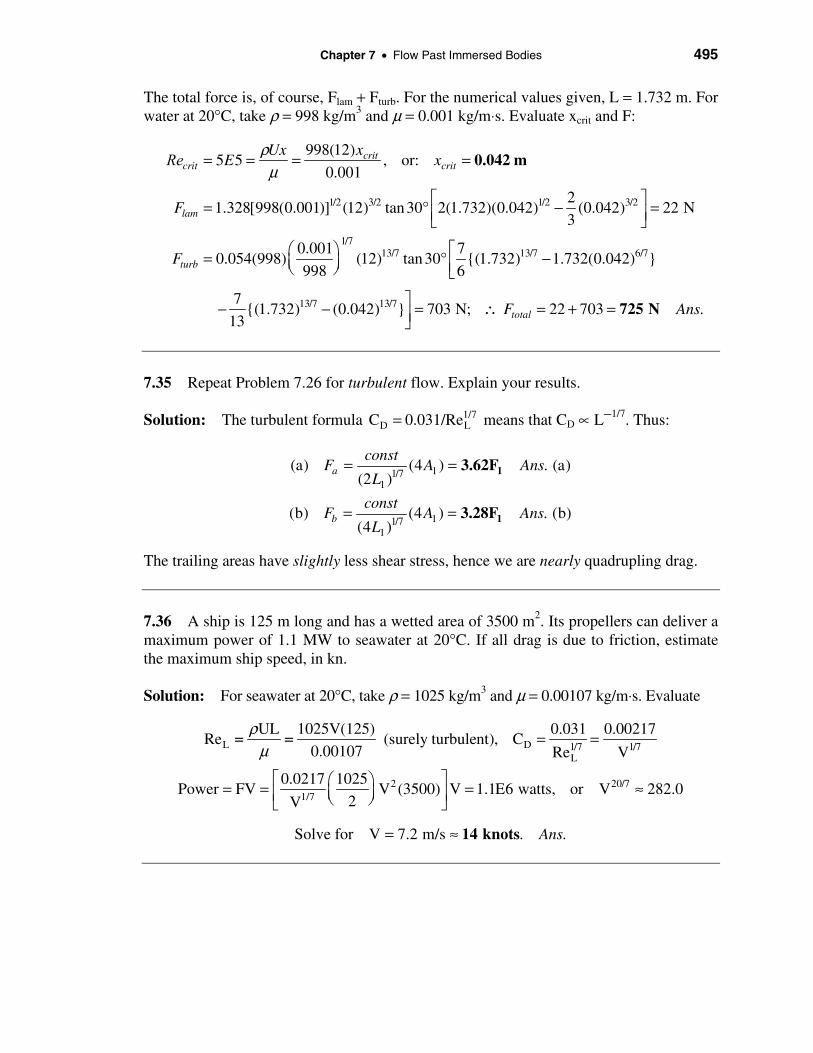
7.35 Repeat Problem 7.26 for turbulent flow. Explain your results.
Solution: The turbulent formula 1/7D LC 0.031/Re= means that CD ∝ L−1/7. Thus:
11/71
(a) (4 ) . (a)(2 )
aconst
F A AnsL
= = 13.62F
11/71
(b) (4 ) . (b)(4 )
bconst
F A AnsL
= = 13.28F
The trailing areas have slightly less shear stress, hence we are nearly quadrupling drag.
7.36 A ship is 125 m long and has a wetted area of 3500 m2. Its propellers can deliver a maximum power of 1.1 MW to seawater at 20°C. If all drag is due to friction, estimate the maximum ship speed, in kn.
Solution: For seawater at 20°C, take ρ = 1025 kg/m3 and µ = 0.00107 kg/m⋅s. Evaluate
L D 1/7 1/7L
2 20/71/7
UL 1025V(125) 0.031 0.00217Re (surely turbulent), C
0.00107 Re V
0.0217 1025Power FV V (3500) V 1.1E6 watts, or V 282.0
2V
ρµ
= =
= = = ≈
= =
Solve for V 7.2 m/s . Ans.= ≈ 14 knots

496 Solutions Manual • Fluid Mechanics, Fifth Edition
7.37 Air at 20°C and 1 atm flows past a long flat plate, at the end of which is placed a narrow scoop, as shown in Fig. P7.37. (a) Estimate the height h of the scoop if it is to extract 4 kg/s per meter of width into the paper. (b) Find the drag on the plate up to the inlet of the scoop, per meter of width.
Fig. P7.37
Solution: For air, take ρ = 1.2 kg/m3 and µ = 1.8E−5 kg/m⋅s. We assume that the scoop does not alter the boundary layer at its entrance. (a) Compute the displacement thickness at x = 6 m:
2 1/7 1/7
6 m
*(30 m/s)(6 m) 1 0.16 0.020Re 1.2 7, 0.00195
80.000015 m /s Re (1.2 7)
* (6 m)(0.00195) 0.0117 m
xx
x
UxE
x E
δν
δ =
= = = ≈ = =
= =|
If δ ∗ were zero, the flow into the scoop would be uniform: 4 kg/s/m = ρUh = (1.2)(30)h, which would make the scoop ho = 0.111 m high. However, we lose the near-wall mass flow ρUδ ∗, so the proper scoop height is equal to
h = ho + δ ∗ = 0.111 m + 0.0117 m ≈ 0.123 m Ans. (a)
(b) Assume Retr = 5E5 and use Eq. (7.49a) to estimate the drag:
1/7
0.031 1440Re 1.2 7, 0.00302 0.00012 0.00290
ReRex d
xx
E C= = − = − =
32 21.2 kg/m
0.0029 (30 m/s) (1 m)(6 m) (b)2 2drag dF C V bL Ans.ρ
= = = 9.4 N
7.38 Atmospheric boundary layers are very thick but follow formulas very similar to those of flat-plate theory. Consider wind blowing at 10 m/s at a height of 80 m above a smooth beach. Estimate the wind shear stress, in Pa, on the beach if the air is standard sea-level conditions. What will the wind velocity striking your nose be if (a) you are standing up and your nose is 170 cm off the ground; (b) you are lying on the beach and your nose is 17 cm off the ground?

Chapter 7 • Flow Past Immersed Bodies 497
Solution: For air at 20°C, take ρ = 1.2 kg/m3 and µ = 1.8E−5 kg/m⋅s. Assume a smooth beach and use the log-law velocity profile, Eq. (7.34), given u = 10 m/s at y = 80 m:
2 2surface
u 10 m/s 1 yu* 1 80u*ln B ln 5.0, solve u* 0.254 m/s
u* u* 0.41 1.5E 5
Hence u* (1.2)(0.254) Ans.
κ ν
τ ρ
= ≈ + = + ≈ −
= = ≈ 0.0772 Pa
The log-law should be valid as long as we stay above y such that yu*/ν > 50:
1.7 mu 1 1.7(0.254)
(a) y 1.7 m: ln 5, solve u (a)0.254 0.41 1.5E 5
Ans.
= ≈ + ≈ −
m7.6
s
17 cmu 1 0.17(0.254)
(b) y 17 cm: ln 5, solve u (b)0.254 0.41 1.5E 5
Ans.
= ≈ + ≈ −
m6.2
s
The (b) part seems very close to the surface, but yu*/ν ≈ 2800 > 50, so the log-law is OK.
7.39 A hydrofoil 50 cm long and 4 m wide moves at 28 kn in seawater at 20°C. Using flat-plate theory with Retr = 5E5, estimate its drag, in N, for (a) a smooth wall and (b) a rough wall, ε = 0.3 mm.
Fig. P7.39
Solution: For seawater at 20°C, take ρ = 1025 kg/m3 and µ = 0.00107 kg/m⋅s. Convert 28 knots = 14.4 m/s. Evaluate ReL = (1025)(14.4)(0.5)/(0.00107) ≈ 6.9E6 (turbulent). Then
D 1/7LL
0.031 1440Smooth, Eq. (7.49a): C 0.00306
ReRe= − ≈
2 2D
1025Drag C U bL(2 sides) (0.00306) (14.4) (4)(0.5)(2) (a)
2 2Ans.
ρ = = ≈
1300 N
DL 500
Rough, 1667, Fig. 7.6 or Eq. (7.48b): C 0.007420.3ε
= = ≈
21025Drag (0.00742) (14.4) (4)(0.5)(2 sides) (b)
2Ans.
= ≈
3150 N
498 Solutions Manual • Fluid Mechanics, Fifth Edition
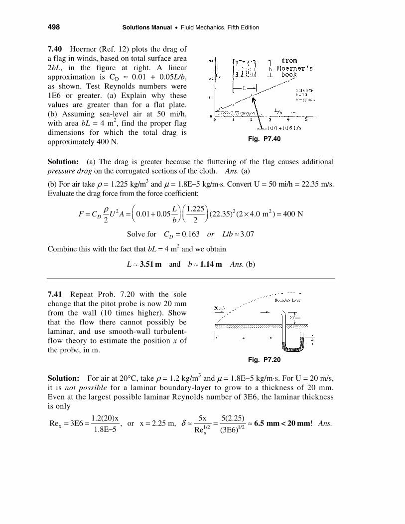
7.40 Hoerner (Ref. 12) plots the drag of a flag in winds, based on total surface area 2bL, in the figure at right. A linear approximation is CD ≈ 0.01 + 0.05L/b, as shown. Test Reynolds numbers were 1E6 or greater. (a) Explain why these values are greater than for a flat plate. (b) Assuming sea-level air at 50 mi/h, with area bL = 4 m2, find the proper flag dimensions for which the total drag is approximately 400 N.
Fig. P7.40
Solution: (a) The drag is greater because the fluttering of the flag causes additional pressure drag on the corrugated sections of the cloth. Ans. (a)
(b) For air take ρ = 1.225 kg/m3 and µ = 1.8E−5 kg/m⋅s. Convert U = 50 mi/h = 22.35 m/s. Evaluate the drag force from the force coefficient:
2 2 21.2250.01 0.05 (22.35) (2 4.0 m ) 400 N
2 2
Solve for 0.163 / 3.07
D
D
LF C U A
b
C or L b
ρ = = + × =
= ≈
Combine this with the fact that bL = 4 m2 and we obtain
and (b)L b Ans.≈ ≈3.51 m 1.14 m
7.41 Repeat Prob. 7.20 with the sole change that the pitot probe is now 20 mm from the wall (10 times higher). Show that the flow there cannot possibly be laminar, and use smooth-wall turbulent-flow theory to estimate the position x of the probe, in m.
Fig. P7.20
Solution: For air at 20°C, take ρ = 1.2 kg/m3 and µ = 1.8E−5 kg/m⋅s. For U = 20 m/s, it is not possible for a laminar boundary-layer to grow to a thickness of 20 mm. Even at the largest possible laminar Reynolds number of 3E6, the laminar thickness is only
x 1/2 1/2x
1.2(20)x 5x 5(2.25)Re 3E6 , or x 2.25 m, ! .
1.8E 5 Re (3E6)Ansδ= = = ≈ = ≈
−6.5 mm < 20 mm

Chapter 7 • Flow Past Immersed Bodies 499
Therefore the flow must be turbulent. Recall from Prob. 7.20 that the manometer reading was h = 16 mm of Meriam red oil, SG = 0.827. Thus
mano pitot2 p m
p gh [0.827(998) 1.2](9.81)(0.016) 129 Pa, u 14.7 s
ρρ∆∆ = ∆ = − ≈ = ≈
1/7 1/7u 14.7 y 20 mm
Then, at y 20 mm, 0.734 , or 174 mmU 20
δδ δ
= = ≈ ≈ = ≈
Thus, crudely, δ/x = 0.174/x ≈ 0.16/Rex1/7, solve for x ≈ 11.6 m. Ans.
7.42 A four-bladed helicopter rotor rotates at n r/min in air with properties (ρ, µ). Each blade has chord length C and extends from the center of rotation out to radius R (the hub size is neglected). Assuming turbulent flow from the leading edge, develop an analytical estimate for the power P required to drive this rotor. (There is no forward velocity.)
Solution: The “freestream” velocity varies linearly from root to tip, as shown in the figure. Thus the drag force on a strip (C dr) of blade is, for turbulent flow,
Fig. P7.42
2 1/7 6/7 6/7 13/71/7C
0.031
dF u C dr (2 sides) 0.031 C ( r) dr, where u r.2Re
ρ µ ρ = ≈ Ω = Ω
R1/7 6/7 6/7 20/7 20/7
blade 0
or Power u dF (4 blades) 4(0.031) C r drµ ρ= = Ω
Finally, after cleaning up, P4 blades ≈ 0.0321µ1/7ρ6/7C6/7Ω20/7R27/7 Ans.
7.43 In the flow of air at 20°C and 1 atm past a flat plate in Fig. P7.43, the wall shear is to be determined at position x by a floating element (a small area connected to a strain-gage force measurement). At x = 2 m, the element indicates a shear stress of 2.1 Pa. Assuming turbulent flow from the
Fig. P7.43
500 Solutions Manual • Fluid Mechanics, Fifth Edition
leading edge, estimate (a) the stream velocity U, (b) the boundary layer thickness δ at the element, and (c) the boundary-layer velocity u, in m/s, at 5 cm above the element.
Solution: For air at 20°C, take ρ = 1.2 kg/m3 and µ = 1.8E−5 kg/m⋅s. The shear stress is
2 22
w f 1/7 1/7
x
0.027 U 0.027 1.2U2.1 Pa C U
2 2 2( Ux/ ) [1.2U(2)/1.8E 5]
Solve for U (a) Check Re 4.54E6 (OK, turbulent)Ans.
ρ ρτρ µ
= = = =
−
≈ ≈m34
s
With the local Reynolds number known, solve for local thickness:
1/7 1/7x
0.16x 0.16(2 m)0.036 m (b)
Re (4.54E6)Ans.δ ≈ = ≈ ≈ 36 mm
Normally, the log-law, Eq. (7.34), is probably best for estimating the velocity at y = 5 cm above the element. However, from Ans. (b) just above, we see that this point is outside the boundary layer. Therefore, the velocity must be u = U ≈ 34 m/s. Ans. (c). [NOTE: Part (c) was supposed to state y = 5 mm, in which case the correct answer would have been u ≈ 26.5 m/s.]
7.44 Extensive measurements of wall shear stress and local velocity for turbulent airflow on the flat surface of the University of Rhode Island wind tunnel have led to the following proposed correlation:
1.772
20.0207wy uyρ τ
νµ ≈
Thus, if y and u(y) are known at a point in a flat-plate boundary layer, the wall shear may be computed directly. If the answer to part (c) of Prob. 7.43 is u ≈ 27 m/s, determine whether the correlation is accurate for this case.
Solution: For air at 20°C, take ρ = 1.2 kg/m3 and µ = 1.8E−5 kg/m⋅s. The shear stress is given as 2.1 Pa, and part (c) was supposed to give y = 5 mm. Check each side of the proposed correlation:
2 2w
2 2
1.771.77
y 1.2(0.005) (2.1);
(1.8E 5)
uy 27(0.005)0.0207 0.0207 (6% more)
1.5E 5
194000
207000
ρ τµ
ν
= ≈−
= ≈ −
The correlation is good and would be even better using a more exact upart(c) ≈ 26.5 m/s.

Chapter 7 • Flow Past Immersed Bodies 501
7.45 A thin sheet of fiberboard weighs 90 N and lies on a rooftop, as shown in the figure. Assume ambient air at 20°C and 1 atm. If the coefficient of solid friction between board and roof is σ = 0.12, what wind velocity will generate enough friction to dislodge the board?
Roof
Fiberboard
2 m 3 m 1 m
1.5 m
2 mU
Fig. P7.45
Solution: For air take ρ = 1.2 kg/m3 and µ = 1.8E−5 kg/m⋅s. Our first problem is to evaluate the drag when the leading edge is not at x = 0. Since the dimensions are large, we will assume that the flow is turbulent and check this later:
( )2 2
1 1
1/72 26/7 6/72 11/7
0.027( /2) 0.031
2( / )
x x
w
x x
U b UF dA b dx x x
UUx
ρ ρ µτρρ µ
= = = −
Set this equal to the dislodging friction force F = σW = 0.12(90) = 10.8 N:
1/72 6/7 6/70.031 1.8 5)
(1.2)(2.0) (5.0 2.0 ) 10.8 N2 1.2
EU
U
− − =
Solve this for U = 33 m/s ≈ 73 mi/h Ans.
1Re 4.4E6: turbulent, OK.x =
7.46 A ship is 150 m long and has a wetted area of 5000 m2. If it is encrusted with barnacles, the ship requires 7000 hp to overcome friction drag when moving in seawater at 15 kn and 20°C. What is the average roughness of the barnacles? How fast would the ship move with the same power if the surface were smooth? Neglect wave drag.
Solution: For seawater at 20°C, take ρ = 1025 kg/m3 and µ = 0.00107 kg/m⋅s. Convert 15 kn = 7.72 m/s. Evaluate ReL = (1025)(7.72)(150)/(0.00107) ≈ 1.11E9 (turbulent). Then
D 2 2
Power 5.22E6 W 2F 2(6.76E5)F 6.76E5 N, C 0.00443
U 7.72 U A 1025(7.72) (5000)ρ= = = = = ≈

502 Solutions Manual • Fluid Mechanics, Fifth Edition
Fig. 7.6 or Eq. (7.48b):
barnaclesL 150
16800, (a)16800
Ans.εε
≈ = ≈ 0.0089 m
If the surface were smooth, we could use Eq. (7.45) to predict a higher ship speed:
22
D 1/7
U 0.031 1025P FU C A U U (5000)U,
2 2[1025U(150) / .00107]
ρ = = =
20/7or: P 5.22E6 watts 5428U , solve for U 11.1 m/s (b)Ans.= = = ≈ 22 knots
7.47 As a case similar to Example 7.5, Howarth also proposed the adverse-gradient velocity distribution U = Uo(1 − x2/L2) and computed separation at xsep/L = 0.271 by a series-expansion method. Compute separation by Thwaites’ method and compare.
Solution: Introduce this freestream velocity into Eq. (7.54), with θo = 0, and integrate:
x2 5 2 2 5
o6 2 2 6o 0
0.45U (1 x /L ) dx,
U (1 x /L )
νθ ≈ −−
22 5
2 60
dU 0.9 xor: (1 ) d ,
dx L(1 )
ηθ ηλ η η ην η
−= = − =−
The result is algebraically complicated but easily solved for the separation point:
4 8 10 122 6 2 65 10 5
0.9 2 (1 ) 0.090 3 7 9 11
at separationη η η ηλ η η η −
= − − + − + − − = −
Solve for ηseparation = 0.268, or: (x/L)sep = 0.268 (within 1%) Ans.
7.48 In 1957 H. Görtler proposed the adverse-gradient test cases
o
(1 / )n
UU
x L=
+
and computed separation for laminar flow at n = 1 to be xsep/L = 0.159. Compare with Thwaites’ method, assuming θo = 0.

Chapter 7 • Flow Past Immersed Bodies 503
Solution: Introduce this stream velocity (n = 1) into Eq. (7.54), with θo = 0, and integrate:
6 5 4x 22 5
6o 0
0.45 x x dU 0.45 x1 U 1 dx, or: 1 1
L L dx 4 LUo
ν θθ λν
− = + + = = − +
sep
xSeparation: 0.09 if ( 1% error)
LAns.λ = − ≈ ≤
0.158
7.49 Based on your understanding of boundary layers, which flow direction (left or right) for the foil shape in the figure will have less total drag?
Fig. P7.49
Solution: Flow to the left has a long run of mild favorable gradient and then a short run of strong adverse gradient—separation and a broad wake will occur, high pressure drag. Flow to the right has a long run of mild adverse gradient—less separation, low pressure drag.
7.50 For flow past a cylinder of radius R as in Fig. P7.50, the theoretical inviscid velocity distribution along the surface is U = 2Uosin(x/R), where Uo is the oncoming stream velocity and x is the arc length measured from the nose (Chap. 8). Compute the laminar separation point xsep and θsep by Thwaites’ method, and compare with the digital-computer solution xsep/R = 1.823 (θsep = 104.5°) given by R. M. Terrill in 1960.
Fig. P7.50
Solution: Introduce this freestream velocity into Eq. (7.54), with θo = 0, and integrate:
22 5 5 o
o6 6o 0
2 46
2U0.45Gn dU dU (2U ) sin (x/R) dx, with , cos(x/R)
dx dx R(2U ) sin (x/R)
0.03cos(x/R) x x xResult: 8 cos 8 4sin 3sin
R R Rsin (x/R)
x θθ λν
λ
= = =
= − + +

504 Solutions Manual • Fluid Mechanics, Fifth Edition
The integral can be found in a good Table of Integrals. Separation then occurs at:
sep180
0.09 at (x/R) 1.7995, or 1.7995
(1.4° less than Terrill’s computation)
Ans.λπ
= − ≈ = ≈
sep 103.1°θ
7.51 Consider the flat-walled diffuser in Fig. P7.51, which is similar to that of Fig. 6.26a with constant width b. If x is measured from the inlet and the wall boundary layers are thin, show that the core velocity U(x) in the diffuser is given approximately by
o
1 (2 tan )/
UU
x Wθ=
+
Fig. P7.51
where W is the inlet height. Use this velocity distribution with Thwaites’ method to compute the wall angle θ for which laminar separation will occur in the exit plane when diffuser length L = 2W. Note that the result is independent of the Reynolds number.
Solution: We can approximate U(x) by the one-dimensional continuity relation:
o oU Wb U(W 2x tan )b, or: U(x) U /[1 2x tan /W] (same as Görtler, Prob. 7.38)θ θ= + ≈ +
We return to the solution from Görtler’s (n = 1) distribution in Prob. 7.38:
2x tan0.09 if 0.158 (separation), or x L 2W,
W
θλ = − = = =
sep0.158
tan 0.0396,4
Ans.θ = = θ sep 2.3≈ °
[This laminar result is much less than the turbulent value θsep ≈ 8° − 10° in Fig. 6.26c.]
7.52 Clift et al. [46] give the formula F ≈ (6π /5)(4 + a/b)µUb for the drag of a prolate spheroid in creeping motion, as shown in Fig. P7.52. The half-thickness b is 4 mm. See also [49]. If the fluid is SAE 50W oil at 20°C, (a) check that Reb < 1; and (b) estimate the spheroid length if the drag is 0.02 N.

Chapter 7 • Flow Past Immersed Bodies 505
Fig. P7.52
Solution: For SAE 50W oil, take ρ = 902 kg/m3 and µ = 0.86 kg/m⋅s. (a) The Reynolds number based on half-thickness is:
3(902 kg/m )(0.2 m/s)(0.004 m)Re 1 (a)
0.86 kg/m sbUb
Ans.ρ
µ= = = <
⋅0.84
(b) With a given force and creeping-flow force formula, we can solve for the half-length a:
6 60.02 4 4 (0.86 kg/m s)(0.20 m/s)(0.004 m)
5 5 0.004
a aF N Ub
b
π πµ = = + = + ⋅
0.0148 m, 2 (b)Solve for a a Ans.= = = Spheroid length 0.030 m
7.53 From Table 7.2, the drag coefficient of a wide plate normal to a stream is approximately 2.0. Let the stream conditions be U∞ and p∞. If the average pressure on the front of the plate is approximately equal to the free-stream stagnation pressure, what is the average pressure on the rear?
Fig. P7.53
Solution: If the drag coefficient is 2.0, then our approximation is
2 2drag plate stag rear plate rear stag
2stag
?F 2.0 U A (p p )A , or: p p U
2
Since, from Bernoulli, p p U , we obtain2
Ans.
ρ ρ
ρ∞ ∞
∞ ∞
= ≈ − ≈ −
= + rearp p U2∞ ∞≈ − ρ 2
7.54 A chimney at sea level is 2 m in diameter and 40 m high and is subjected to 50 mi/h storm winds. What is the estimated wind-induced bending moment about the bottom of the chimney?

506 Solutions Manual • Fluid Mechanics, Fifth Edition
Solution: For sea-level air, take ρ = 1.225 kg/m3 and µ = 1.78E−5 kg/m⋅s. Convert 50 mi/h = 22.35 m/s. Evaluate the Reynolds number and drag coefficient for a cylinder:
D DUD 1.225(22.35)(2)
Re 3.08E6 (turbulent); Fig. 7.16a: C 0.4 0.11.78E 5
ρµ
= = ≈ ≈ ±−
2 2drag D
1.225Then F C U DL 0.4 (22.35) (2)(40) (a)
2 2Ans.
ρ = = ≈
10, 000 N
oRoot bending moment M FL/2 (10000)(40/2) (b)Ans.≈ = ≈ 200,000 N m⋅
7.55 A ship tows a submerged cylinder, 1.5 m in diameter and 22 m long, at U = 5 m/s in fresh water at 20°C. Estimate the towing power in kW if the cylinder is (a) parallel, and (b) normal to the tow direction.
Solution: For water at 20°C, take ρ = 998 kg/m3 and µ = 0.001 kg/m⋅s.
L D,frontalL 998(5)(22)
(a) Parallel, 15, Re 1.1E8, Table 7.3: estimate C 1.1D 0.001
≈ = = ≈
2 2998F 1.1 (5) (1.5) 24000 N, Power FU (a)
2 4Ans.
π = ≈ = ≈
120 kW
D D,frontal998(5)(1.5)
(b) Normal, Re 7.5E6, Fig. 7.16a: C 0.40.001
= = ≈
2998F 0.4 (5) (1.5)(22) 165000 N, Power FU (b)
2Ans.
= ≈ = ≈
800 kW
7.56 A delivery vehicle carries a long sign on top, as in Fig. P7.56. If the sign is very thin and the vehicle moves at 65 mi/h, (a) estimate the force on the sign with no crosswind. (b) Discuss the effect of a crosswind.
Fig. P7.56

Chapter 7 • Flow Past Immersed Bodies 507
Solution: For air at 20°C, take ρ = 1.2 kg/m3 and µ = 1.8E−5 kg/m⋅s. Convert 65 mi/h = 29.06 m/s. (a) If there is no crosswind, we may estimate the drag force by flat-plate theory:
1/7 1/7
2 2
1.2(29.06)(8) 0.031 0.031Re 1.55 7 ( ), 0.00291
1.8 5 Re (1.55 7)
1.2(2 ) 0.00291 (29.06) (0.6)(8)(2 ) . (a)
2 2
L DL
drag D
E turbulent CE E
F C V bL sides sides Ansρ
= = = = ≈−
= = = 14 Ν
(b) A crosswind will cause a large side force on the sign, greater than the flat-plate drag. The sign will act like an airfoil. For example, if the 29 m/s wind is at an angle of only 5° with respect to the sign, from Eq. (7.70), CL ≈ 2π sin (5°)/(1 + 2/.075) ≈ 0.02. The lift on the sign is then about
Lift = CL (ρ/2)V 2bL ≈ (0.02)(1.2/2)(29.06)2(0.6)(8) ≈ 50 N Ans. (b)
7.57 The main cross-cable between towers of a coastal suspension bridge is 60 cm in diameter and 90 m long. Estimate the total drag force on this cable in crosswinds of 50 mi/h. Are these laminar-flow conditions?
Solution: For air at 20°C, take ρ = 1.2 kg/m3 and µ = 1.8E−5 kg/m⋅s. Convert 50 mi/h = 22.35 m/s. Check the Reynolds number of the cable:
D D1.2(22.34)(0.6)
Re 894000 (turbulent flow) Fig. 7.16a: C 0.31.8E 5
= ≈ ≈−
2 2drag D
1.2F C U DL 0.3 (22.35) (0.6)(90) ( )
2 2Ans.
ρ = = ≈ 5000 N not laminar
7.58 A long cylinder of rectangular cross section, 5 cm high and 30 cm long, is immersed in water at 20°C flowing at 12 m/s parallel to the long side of the rectangle. Estimate the drag force on the cylinder, per unit length, if the rectangle (a) has a flat face or (b) has a rounded nose.
Fig. P7.58

508 Solutions Manual • Fluid Mechanics, Fifth Edition
Solution: For water at 20°C, take ρ = 998 kg/m3 and µ = 0.001 kg/m⋅s. Assume a two-dimensional flow, i.e., use Table 7.2. If the nose is flat, L/H = 6, then CD ≈ 0.9:
2 2D
998Flat nose: F C U H(1 m) 0.9 (12) (0.05) (a)
2 2Ans.
ρ = = ≈
N3200
m
D flat0.64
Round nose, Table 7.2: C 0.64, F F (b)0.9
Ans.≈ = ≈ N2300
m
7.59 Joe can pedal his bike at 10 m/s on a straight, level road with no wind. The bike rolling resistance is 0.80 N/(m/s), i.e. 0.8 N per m/s of speed. The drag area CDA of Joe and his bike is 0.422 m2. Joe’s mass is 80 kg and the bike mass is 15 kg. He now encounters a head wind of 5.0 m/s. (a) Develop an equation for the speed at which Joe can pedal into the wind. (Hint: A cubic equation.) (b) Solve for V for this head wind. (c) Why is the result not simply V = 10 − 5 = 5 m/s, as one might first suspect?
Solution: Evaluate force and power with the drag based on relative velocity V + Vwind:
2
2 2
( )2
( )2
rolling drag RR D wind
RR D wind
F F F C V C A V V
Power V F C V C A V V V
ρ
ρ
= + = + +
= = + +
Let Vnw (=10 m/s) be the bike speed with no wind and denote Vrel = V + Vwind. Joe’s power output will be the same with or without the headwind:
( )
2 3 2 2
3 2 2 3 2
,2 2
2 2: 2 0 (a)
nw RR nw D nw RR D rel
RR RRw w nw nw
D D
P C V C A V P C V C A VV
C Cor V V V V V V V Ans.
C A C A
ρ ρ
ρ ρ
= + = = +
+ + + − + =
For our given numbers, assuming ρair = 1.2 kg/m3, the result is the cubic equation
3 213.16 25 1316 0, (b)V V V solve for Ans.+ + − = mV 7.4
s≈
Since drag is proportional to 2relV , a linear transformation V = Vnw − Vwind is not
possible. Even if there were no rolling resistance, V ≈ 7.0 m/s, not 5.0 m/s. Ans. (c)

Chapter 7 • Flow Past Immersed Bodies 509 7.60 A fishnet consists of 1-mm-diameter strings overlapped and knotted to form 1- by 1-cm squares. Estimate the drag of 1 m2 of such a net when towed normal to its plane at 3 m/s in 20°C seawater. What horsepower is required to tow 400 ft2 of this net?
Fig. P7.60
Solution: For seawater at 20°C, take ρ =1025 kg/m3 and µ = 0.00107 kg/m⋅s. Neglect the knots at the net’s intersections. Estimate the drag of a single one-centimeter strand:
D D
2 2one strand D
1025(3)(0.001)Re 2900; Fig. 7.16a or Fig. 5.3a: C 1.0
0.001071025
F C U DL (1.0) (3) (0.001)(0.01) 0.046 N/strand2 2
ρ
= ≈ ≈
= = ≈
21 sq mone m contains strands: F 20000(0.046) (a)20,000 Ans.≈ ≈ 920 N
2 2To tow 400 ft 37.2 m of net, F 37.2(920) 34000 N 7700 lbf= = ≈ ≈
m ftIf U 3 9.84 , Tow Power FU (7700)(9.84) 550 (b)
s sAns.= = = = ÷ ≈ 140 hp
7.61 A filter may be idealized as an array of cylindrical fibers normal to the flow, as in Fig. P7.61. Assuming that the fibers are uniformly distributed and have drag coef-ficients given by Fig 7.16a, derive an approximate expression for the pressure drop ∆p through a filter of thickness L.
Solution: Consider a filter section of height H and width b and thickness L. Let N be the number of fibers of diameter D per
Fig. P7.61
unit area HL of filter. Then the drag of all these filters must be balanced by a pressure ∆p across the filter:
2fibers D filterpHb F NHLC U Db , or: p
2Ans.
ρ∆ = = ∆ ≈ 2DNLC U D
2ρ
This simple expression does not account for the blockage of the filters, that is, in cylinder arrays one must increase “U” by 1/(1 − σ), where σ is the solidity ratio of the filter.

510 Solutions Manual • Fluid Mechanics, Fifth Edition
7.62 A sea-level smokestack is 52 m high and has a square cross-section. Its supports can withstand a maximum side force of 90 kN. If the stack is to survive 90 mi/h hurricane winds, what is its maximum possible (square) width?
Solution: For sea-level air, take ρ = 1.225 kg/m3 and µ = 1.78E−5 kg/m⋅s. Convert 90 mi/h = 40.2 m/s. We cannot compute Re without knowing the side length a, so we assume that Re > 1E4 and that Table 7.2 is valid. The worst case drag is when the square cylinder has its flat face forward, CD ≈ 2.1. Then the drag force is
2 2D
?1.225F C U aL 2.1 (40.2) a(52) 90000 N, solve
2 2Ans.
ρ = = = a 0.83 m≈
Check Rea = (1.225)(40.2)(0.83)/(1.78E−5) ≈ 2.3E6 > 1E4, OK.
7.63 For those who think electric cars are sissy, Keio University in Japan has tested a 22-ft long prototype whose eight electric motors generate a total of 590 horsepower. The “Kaz” cruises at 180 mi/h (see Popular Science, August 2001, p. 15). If the drag coefficient is 0.35 and the frontal area is 26 ft2, what percent of this power is expended against sea-level air drag?
Solution: For air, take ρ = 0.00237 slug/ft3. Convert 180 mi/h to 264 ft/s. The drag is
32 2 20.00237 slug/ft
(0.35) (264 ft/s) (26 ft ) 752 lbf2 2D frontalF C V Aρ
= = =
(752 lbf)(264 ft/s)/(550 ft lbf/hp)Power FV= = ⋅ = 361 hp
The horsepower to overcome drag is 61% of the total 590 horsepower available. Ans.
7.64 A parachutist jumps from a plane, using an 8.5-m-diameter chute in the standard atmosphere. The total mass of chutist and chute is 90 kg. Assuming a fully open chute in quasisteady motion, estimate the time to fall from 2000 to 1000 m.
Solution: For the standard altitude (Table A-6), read ρ = 1.112 kg/m3 at 1000 m altitude and ρ = 1.0067 kg/m3 at 2000 meters. Viscosity is not a factor in Table 7.3, where we read CD ≈ 1.2 for a low-porosity chute. If acceleration is negligible,
2 2 2 2 2 25.93, : 90(9.81) 1.2 (8.5) , :
2 4 2 4DW C U D or N U or Uρ π ρ π
ρ = = =

Chapter 7 • Flow Past Immersed Bodies 511
1000 2000 25.93 25.93
Thus and 1.1120 1.0067m mU U= = = =m m
4.83 5.08s s
Thus the change in velocity is very small (an average deceleration of only −0.001 m/s2) so we can reasonably estimate the time-to-fall using the average fall velocity:
2000 1000
(4.83 5.08)/2fallavg
zt Ans.
V
∆ −∆ = = ≈+
202 s
7.65 As soldiers get bigger and packs get heavier, a parachutist and load can weigh as much as 400 lbf. The standard 28-ft parachute may descend too fast for safety. For heavier loads, the U.S. Army Natick Center has developed a 28-ft, higher drag, less porous XT-11 parachute (see the URL http://www.natick.army.mil). This parachute has a sea-level descent speed of 16 ft/s with a 400-lbf load. (a) What is the drag coefficient of the XT-11? (b) How fast would the standard chute descend at sea-level with such a load?
Solution: For sea-level air, take ρ = 0.00237 slug/ft3. (a) Everything is known except CD: 3
2 2 20.00237 slug/ft400 lbf (16 ft/s) (28 ft)
2 2 4D DF C V A Cρ π= = =
, (a)D new chuteSolve for C Ans.= 2.14
(b) From Table 7.3, a standard chute has a drag coefficient of about 1.2. Then solve for V:
32 2 20.00237 slug/ft
400 lbf (1.2) (28 ft)2 2 4DF C V A Vρ π= = =
(b)old chuteSolve for V Ans.= 21.4 ft/s
7.66 A sphere of density ρs and diameter D is dropped from rest in a fluid of density ρ and viscosity µ. Assuming a constant drag coefficient o ,dC derive a differential equation for the fall velocity V(t) and show that the solution is
o
1/ 24 ( 1)
tanh3 d
gD SV Ct
C
−=
o
1/ 2
2
3 ( 1)
4dgC S
CS D
− =
Fig. P7.66
where S = ρs/ρ is the specific gravity of the sphere material.

512 Solutions Manual • Fluid Mechanics, Fifth Edition
Solution: Newton’s law for downward motion gives
2 2down down D
3 2
D
W dVF ma , or: W B C V A , where A D
2 g dt 4
dVand W B (S 1)g D . Rearrange to V ,
6 dt
1 gC Ag 1 and
S 2W
ρ π
πρ β α
ρβ α
= − − = =
− = − = −
= − =
Separate the variables and integrate from rest, V = 0 at t = 0: dt = dV/(β − αV2),
( )or: V tanh t Ans.β αβα
= = finalV tanh(Ct)
1/2 1/2sD
final 2D
4gD(S 1) 3gC (S 1)where V and C , S 1
3C 4S D
ρρ
− − = = = >
7.67 A world-class bicycle rider can generate one-half horsepower for long periods. If racing at sea-level, estimate the velocity which this cyclist can maintain. Neglect rolling friction.
Solution: For sea-level air, take ρ = 1.22 kg/m3. From Table 7.3 for a bicycle with a rider in the racing position, CDA ≈ 0.30 m2. With power known, we can solve for speed:
32 2 31.22 kg/m
0.5 hp 373 (0.3 m )2 2DPower FV C A V V W Vρ = = = = =
Solve for V Ans.= about 12.7 m/s ( 28 mi/h)
7.68 A baseball weighs 145 g and is 7.35 cm in diameter. It is dropped from rest from a 35-m-high tower at approximately sea level. Assuming a laminar-flow drag coefficient, estimate (a) its terminal velocity and (b) whether it will reach 99 percent of its terminal velocity before it hits the ground.

Chapter 7 • Flow Past Immersed Bodies 513
Solution: For sea-level air, take ρ = 1.225 kg/m3 and µ = 1.78E−5 kg/m⋅s. Assume a laminar drag coefficient CD ≈ 0.47 from Table 7.3. The terminal velocity is
final 2 2D
2W 2[0.145(9.81)]V . (a)
C ( /4)D 0.47(1.225)( /4)(0.0735)Ans
ρ π π= = ≈ m
34.1s
Now establish the “specific gravity” of the ball, relative to air:
ballball 3 3
air
m 0.145 kg 697.4697.4 , “S”
1.225( /6)(0.0735) m
ρρυ ρπ
= = = = = = 569
Then the constant C from Prob. 7.66 gives the time history of velocity and displacement:
1/21/21D
f2 2
D
3gC (S 1) 3(9.81)(0.47)(569 1)C 0.287 s , V V tanh(Ct),
4S D 4(569) (0.0735)
34.1or: V 34.1tanh (0.287t), Z V dt ln[ cosh (0.287t)]
0.287
Check Re (max) 1.225(34.1)(0.0735)/(1.78E 5) 172000 (OK
− − − = = ≈ =
= = =
= − ≈
D, C 0.47)≈
We can now find the time and velocity when the balls hits Z = 35 m:
34.1Z 35 ln[cosh(0.287t)], solve for t , whence
0.287= = ≈ 2.81 s
V(at Z 35 m) 34.1tanh[0.287(2.81)] (b)Ans.= = ≈ m22.8
s
This is only 67% of terminal velocity. If we try the formulas again for V = 99% of terminal velocity (about 33.8 m/s), we find that t ≈ 9.22 s and Z ≈ 230 m.
7.69 Two baseballs from Prob. 7.68 are connected to a rod 7 mm in diameter and 56 cm long, as in Fig. P7.69. What power, in W, is required to keep the system spinning at 400 r/min? Include the drag of the rod, and assume sea-level standard air.
Fig. P7.69

514 Solutions Manual • Fluid Mechanics, Fifth Edition
Solution: For sea-level air, take ρ = 1.225 kg/m3 and µ = 1.78E−5 kg/m⋅s. Assume a laminar drag coefficient CD ≈ 0.47 from Table 7.3. Convert Ω = 400 rpm × 2π /60 = 41.9 rad/s. Each ball moves at a centerline velocity
b b
D
V r (41.9)(0.28 0.0735/2) 13.3 m/s
Check Re 1.225(13.3)(0.0735)/(1.78E 5) 67000; Table 7.3: C 0.47
= Ω = + ≈
= − ≈ ≈
Then the drag force on each baseball is approximately
2 2 2 2b D b
1.225F C V D 0.47 (13.3) (0.0735) N
2 4 2 40.215
ρ π π = = ≈
Make a similar approximate estimate for the drag of each rod:
r avg D
2 2rod D r
m 1.225(5.86)(0.007)V r 41.9(0.14) 5.86 , Re 2800, C 1.2
s 1.78E 5
1.225F C V DL 1.2 (5.86) (0.007)(0.28) N
2 20.0495
ρ
= Ω = ≈ = ≈ ≈−
≈ = ≈
Then, with two balls and two rods, the total driving power required is
b b r rP 2F V 2F V 2(0.215)(13.3) 2(0.0495)(5.86) 5.71 0.58 Ans.= + = + = + ≈ 6.3 W
7.70 A baseball from Prob. 7.68 is batted upward during a game at an angle of 45° and an initial velocity of 98 mi/h. Neglect spin and lift. Estimate the horizontal distance traveled, (a) neglecting drag and (b) accounting for drag in a numerical (computer) solution with a transition Reynolds number ReD,crit = 2.5E5.
Fig. P7.70
Solution: (a) Convert 98 mi/h = 43.8 m/s. For zero drag, we make use of the simple physics formulas for particles:
2 22 2o oXD
max2(V cos45 ) V2V (43.8)
x L 196 m (a)g g g 9.81
Ans.°∆ = = = = = = = 642 ft

Chapter 7 • Flow Past Immersed Bodies 515
(b) With drag of a sphere (CD ≈ 0.47) included, we need to use Newton’s law in both the x- and z-directions. With reference to the trajectory figure shown, we derive the nonlinear equations of motion of the ball with constant drag coefficient:
( )2
2 2 2x x D x z2
2 2 1z z z x
d xF ma , or: 0.145 F cos , where F C D V V
2 4dt
F ma , or: 0.145 d z/dt F sin W, where tan (V /V )
ρ πθ
θ θ −
= = − = +
= = − − =
Assume mg = W = 0.145(9.81) = 1.42 N, ρ = 1.225 kg/m3, D = 0.0735 m, and Vx(0) = Vz(0) = 43.8(0.707) = 31.0 m/s. Integrate numerically, by Runge-Kutta or whatever, for x(t) and z(t), until the ball comes back down again and z = 0. The Reynolds number is in the transition range, ReD ≈ 222000. Most probably, due to ball/stitch roughness, CD ≈ 0.2 (turbulent). We have also carried out the integration for CD ≈ 0.47 (laminar). The results are:
D DC 0.2: L 130 m (b); or: C 0.47: L 92 m ft.Ans. 303= ≈ ≈ = ≈ ≈425 ft
7.71 A football weights 0.91 lbf and approximates an ellipsoid 6 in in diameter and 12 in long (Table 7.3). It is thrown upward at a 45° angle with an initial velocity of 80 ft/s. Neglect spin and lift. Assuming turbulent flow, estimate the horizontal distance traveled, (a) neglecting drag and (b) accounting for drag with a numerical (computer) model.
Fig. P7.71
Solution: For sea-level air, take ρ = 0.00238 slug/ft3 and µ = 3.71E−7 slug/ft⋅s. For a 2:1 ellipsoid, in Table 7.3, assume CD ≈ 0.13 (turbulent flow). (a) For zero drag, we make use of the simple physics formulas for particles:
2 2 2max o ox L 2(V cos 45 ) /g V /g (80) /32.2 (a)Ans.∆ = = ° = = ≈ 199 ft
(b) With drag of an ellipsoid (CD ≈ 0.13) included, we need to use Newton’s law in both the x- and z-directions. With reference to the figure above, we derive the nonlinear equations of motion of the ball with constant drag coefficient:
( )2 2 2xx x D x z
1zz z z x
0.91 dVF ma , or: F cos , where F C V V D
32.2 dt 2 4
0.91 dVF ma , or: F sin W, where tan (V /V )
32.2 dt
ρ πθ
θ θ −
= = − = +
= = − − =

516 Solutions Manual • Fluid Mechanics, Fifth Edition
Assume W = 0.91 lbf, ρ = 0.00238 slug/ft3, D = 0.5 ft, and Vx (0) = Vz(0) = 80(0.707) = 56.6 ft/s. Integrate numerically, by Runge-Kutta or whatever, for x(t) and z(t), until the ball comes back down again and z = 0. The results are:
max maxx L at t 3.4 s (z 46 ft) (b)Ans.∆ = ≈ = ≈171 ft
7.72 A settling tank for a municipal water supply is 2.5 m deep, and 20°C water flows through continuously at 35 cm/s. Estimate the minimum length of the tank which will ensure that all sediment (SG = 2.55) will fall to the bottom for particle diameters greater than (a) 1 mm and (b) 100 µm.
Fig. P7.72
Solution: For water at 20°C, take ρ = 998 kg/m3 and µ = 0.001 kg/m⋅s. The particles travel with the stream flow U = 35 cm/s (no horizontal drag) and fall at speed Vf with drag equal to their net weight in water:
3 2 2 2wnet w D f f
D
4(SG 1)gDW (SG 1) g D Drag C V D , or: V
6 2 4 3C
ρπ πρ −= − = = =
where CD = fcn(ReD) from Fig. 7.16b. Then L = Uh/Vf where h = 2.5 m.
2f D
D
4(2.55 1)(9.81)(0.001)(a) D 1 mm: V , iterate Fig. 7.16b to C 1.0,
3C
−= = ≈
D f f(0.35)(2.5)
Re 140, V 0.14 m/s, hence L Uh/V (a)0.14
Ans.≈ ≈ = = ≈ 6.3 m
2f D
D
4(2.55 1)(9.81)(0.0001)(b) D 100 m: V , iterate Fig. 7.16b to C 36,
3Cµ −= = ≈
D f0.35(2.5)
Re 0.75, V 0.0075 m/s, L (b)0.0075
Ans.≈ ≈ = ≈ 120 m

Chapter 7 • Flow Past Immersed Bodies 517
7.73 A balloon is 4 m in diameter and contains helium at 125 kPa and 15°C. Balloon material and payload weigh 200 N, not including the helium. Estimate (a) the terminal ascent velocity in sea-level standard air; (b) the final standard altitude (neglecting winds) at which the balloon will come to rest; and (c) the minimum diameter (<4 m) for which the balloon will just barely begin to rise in sea-level air.
Solution: For sea-level air, take ρ = 1.225 kg/m3 and µ = 1.78E−5 kg/m⋅s. For helium R = 2077 J/kg⋅°K. Sea-level air pressure is 101350 Pa. For upward motion V,
3 2 2
3 2 2
, : ( )6 2 4
125000 1.225: 1.225 (9.81) (4) 200 (4)
2077(288) 6 2 4
air He D
D
Net buoyancy weight drag or g D W C V D
or C V
π ρ πρ ρ
π π
= + − = +
− = +
DGuess flow: C 0.2: Solve for (a)turbulent Ans.≈ V 9.33 m/s≈
Check ReD = 2.6E6: OK, turbulent flow.
(b) If the balloon comes to rest, buoyancy will equal weight, with no drag:
3
3
125000 (9.81) (4) 200,
2077(288) 6
kgSolve: 0.817 , (b)
m
air
air Ans.
πρ
ρ
− =
≈ Table A6Z 4000 m≈
(c) If it just begins to rise at sea-level, buoyancy will be slightly greater than weight:
31250001.225 (9.81) 200, : (c)
2077(288) 6D or Ans.
π − >
D > 3.37 m
7.74 It is difficult to define the “frontal area” of a motorcycle due to its complex shape. One then measures the drag-area, that is, CDA, in area units. Hoerner [12] reports the drag-area of a typical motorcycle, including the (upright) driver, as about 5.5 ft2. Rolling friction is typically about 0.7 lbf per mi/h of speed. If that is the case, estimate the maximum sea-level speed (in mi/h) of the new Harley-Davidson V-RodΟ cycle, whose liquid-cooled engine produces 115 hp.
Solution: For sea-level air, take ρ = 0.00237 slug/ft3. Convert 0.7 lbf per mi/h rolling friction to 0.477 lbf per ft/s of speed. Then the power relationship for the cycle is
2( ) ,2dr roll D rollPower F F V C A V C V Vρ = + = +
518 Solutions Manual • Fluid Mechanics, Fifth Edition
32 2ft-lbf 0.00237 slug/ft lbf
or: 115*550 (5.5 ft ) 0.477 s 2 ft/s
V V V
= +
Solve this cubic equation, by iteration or EES, to find Vmax ≈ 192 ft/s ≈ 131 mi/h. Ans.
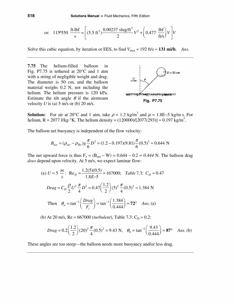
7.75 The helium-filled balloon in Fig. P7.75 is tethered at 20°C and 1 atm with a string of negligible weight and drag. The diameter is 50 cm, and the balloon material weighs 0.2 N, not including the helium. The helium pressure is 120 kPa. Estimate the tilt angle θ if the airstream velocity U is (a) 5 m/s or (b) 20 m/s.
Fig. P7.75
Solution: For air at 20°C and 1 atm, take ρ = 1.2 kg/m3 and µ = 1.8E−5 kg/m⋅s. For helium, R = 2077 J/kg⋅°K. The helium density = (120000)/[2077(293)] ≈ 0.197 kg/m3.
The balloon net buoyancy is independent of the flow velocity:
3 3( ) (1.2 0.197)(9.81) (0.5) 0.644 N6 6net air HeB g Dπ πρ ρ= − = − ≈
The net upward force is thus Fz = (Bnet − W) = 0.644 − 0.2 = 0.444 N. The balloon drag does depend upon velocity. At 5 m/s, we expect laminar flow:
1.2(5)(0.5)(a) 5 : Re 167000; 7.3: 0.47
1.8 5D Dm
U Table Cs E
= = = ≈−
2 2 2 21.20.47 (5) (0.5) 1.384 N
2 4 2 4DDrag C U Dρ π π = = ≈
1 1 1.384Then tan tan (a)
0.444az
DragAns.
Fθ − − = = =
72°
(b) At 20 m/s, Re = 667000 (turbulent), Table 7.3: CD ≈ 0.2:
2 2 11.2 9.430.2 (20) (0.5) 9.43 N, tan (b)
2 4 0.444bDrag Ans.π θ − = = = =
87°
These angles are too steep—the balloon needs more buoyancy and/or less drag.

Chapter 7 • Flow Past Immersed Bodies 519
7.76 Extend Problem 7.75 to make a smooth plot of tilt angle θ versus stream velocity U in the range 1 < U < 12 mi/h (use a spreadsheet). Comment on the effectiveness of this system as an air-velocity instrument.
Solution: The spreadsheet calculates the drag and divides by the constant upward force of 0.444 N to calculate and plot the angle:
2 21 ( /2) ( /4)
( ) tan , (Re )0.444 N
DD D
C U Dfcn U C fcn
ρ πθ − = = =
The results are shown in the plot given below. At these velocities, all Reynolds numbers are less than 200,000, so a smooth sphere will be laminar, CD ≈ 0.47. We see that the plot, in principle, shows a nice spread of angles, from zero to 74 degrees, for these velocities. However, because of the unsteady, pulsating nature of the wake of a sphere in a stream, the balloon would no doubt oscillate in the stream and the tilt angle would be difficult to estimate accurately.
Problem 7.76: Balloon Tilt Angle Versus Flow Velocity
7.77 To measure the drag of an upright person, without violating human-subject protocols, a life-sized mannequin is attached to the end of a 6-m rod and rotated at Ω = 80 rev/min, as in Fig. P7.77. The power required to maintain the rotation is 60 kW. By including rod-drag power, which is significant, estimate the drag-area CDA of the mannequin, in m2.

520 Solutions Manual • Fluid Mechanics, Fifth Edition
Fig. P7.77
Solution: For air, take ρ = 1.2 kg/m3 and µ = 1.8E−5 kg/m⋅s. The mannequin velocity is Vm = ΩL = [(80 × 2π/60)rad/s](6m) ≈ (8.38 rad/s)(6 m) ≈ 50.3 m/s. The velocity at mid-span of the rod is ΩL/2 = 25 m/s. Crudely estimate the power to rotate the rod:
,2
42 2 2
0
42
(25 m/s)(0.08 m)Re 133000, 7.2: 1.2
0.000015 m /s
2 2 4
1.2 6.0Input the data: (1.2) (8.38) (0.08) 1300
2 4
D D rod
L
rod D D
rod
VDTable C
v
LP C r D dr r C D
P W
ρ ρ
= = = ≈
≈ Ω ≈ Ω
= ≈
Rod power is thus only about 2% of the total power. The total power relation is:
3 31.2( ) 1300 ( ) (50.3) 60000
2 2rod D man D manP P C A V C A Wρ = + = + =
Solve for Ans.2D mannequin(C A) 0.77 m≈
7.78 Apply Prob. 7.61 to a filter consisting of 300-µm-diameter fibers packed 250 per square centimeter in the plane of Fig. P7.61. For air at 20°C and 1 atm flowing at 1.5 m/s, estimate the pressure drop if the filter is 5 cm thick.
Fig. P7.61
Solution: For air at 20°C and 1 atm, take ρ = 1.2 kg/m3 and µ = 1.8E−5 kg/m⋅s. In Prob. 7.61 we derived the pressure-drop expression
2filter Dp NLC U D, where N no. of fibers per unit area
2
ρ∆ ≈ =

Chapter 7 • Flow Past Immersed Bodies 521
Here, N = 250/cm2 = 2.5E6 per square meter (about 18% solidity). The drag coefficient is based on the Reynolds number (here uncorrected for solidity):
D DUD 1.2(1.5)(0.0003)
Re 30; Fig. 7.16a: C1.8E 5
2.0ρ
µ= = ≈ ≈
−
2 2D
1.2Then p NLC U D (2.5E6)(0.05)(2.0) (1.5) (0.0003) .
2 2Ans
ρ ∆ ≈ = ≈
100 Pa
7.79 A radioactive dust particle approximate a sphere with a density of 2400 kg/m3. How long, in days, will it take the particle to settle to sea level from 12 km altitude if the particle diameter is (a) 1 µm; (b) 20 µm?
Solution: For such small particles, tentatively assume that Stokes’ law prevails:
3 3 3drag net p air
3 2fall
F DV W ( )g D (2400 1 or so)(9.81) D 12320D6 6
Thus V (12320D )/[3 D ] 1307D / dZ/dt, where Z altitude
π ππµ ρ ρ
π µ µ
≈ 3 = = − = − ≈
≈ ≈ = − =
Thus the time to fall varies inversely as D2 and depends on an average viscosity in the air:
12000
fall avg 0-12000 avg2 20
1 12000 kgt dZ , Table A-6 gives 1.61E 5
m·s1307D 1307Dµ µ µ∆ = = | ≈ −
Try our two different diameters and check the Reynolds number for Stokes’ flow:
2
12000(1.61E 5)(a) D 1 m: t 1.48E8 s (a)
1307(1E 6)Ans.µ −= ∆ = ≈ ≈
−1710 days
maxRe 5E 6 1, OK≈ −
2
12000(1.61E 5)(b) D 20 m: t 3.70E5 s (b)
1307(2E 5)Ans.µ −= ∆ = ≈ ≈
−4.3 days
maxRe 0.04 1, OK≈

522 Solutions Manual • Fluid Mechanics, Fifth Edition
7.80 A heavy sphere attached to a string should hang at an angle θ when immersed in a stream of velocity U, as in Fig. P7.80. Derive an expression for θ as a function of the sphere and flow properties. What is θ if the sphere is steel (SG = 7.86) of diameter 3 cm and the flow is sea-level standard air at U = 40 m/s? Neglect the string drag.
Solution: For sea-level air, take ρ = 1.225 kg/m3 and µ = 1.78E−5 kg/m⋅s. The sphere should hang so that string tension balances the resultant of drag and net weight:
Fig. P7.80
31net s
2 2D
W ( )g( /6)Dtan , or tan .
Drag ( /8)C U DSymbolic answer
ρ ρ πθ θπ ρ
− −= =
For the given numerical data, first check Re and the drag coefficient, then find the angle:
D D1.225(40)(0.03)
Re 83000, Fig. 7.16b: C1.78E 5
= ≈ ≈−
0.5
2 2
3 1
F (0.5)(1.225)(40) (0.03) 0.346 N;8
W [7.86(998) 1.225](9.81) (0.03) 1.09 N tan (1.09/0.346)6
Ans.
π
π θ −
= ≈
= − ≈ ∴ = ≈ 72°
7.81 A typical U.S. Army parachute has a projected diameter of 28 ft. For a payload mass of 80 kg, (a) what terminal velocity will result at 1000-m standard altitude? For the same velocity and payload, what size drag-producing “chute” is required if one uses a square flat plate held (b) vertically; and (c) horizontally? (Neglect the fact that flat shapes are not dynamically stable in free fall.) Neglect plate weight.
Solution: For air at 1000 meters, from Table A-3, ρ ≈ 1.112 kg/m3. Convert D = 28 ft = 8.53 m. Convert W = mg = 80(9.81) = 785 N. From Table 7-3 for a parachute, read CD ≈ 1.2, Then, for part (a),
2 21.112785 N 1.2 (8.53) , solve for (a)
2 4W Drag U U Ans.
π = = = ≈
m4.53
s
Chapter 7 • Flow Past Immersed Bodies 523
(c) From Table 7-3 for a square plate normal to the stream, read CD ≈ 1.18. Then
2 21.112785 N 1.18 (4.53) , solve for 7.63 (c)
2W Drag L L m Ans.
= = = ≈ = 25 ft
This is a comparable size to the parachute, but a square plate is ungainly and unstable.
(b) For a square plate parallel to the stream use (turbulent) flat plate theory. We need the viscosity—at 1000 meters altitude, estimate µair ≈ 1.78E−5 kg/m⋅s. Then
2 21/7
0.031 1.112785 N (4.53) (2 )
2[1.112(4.53) /1.78 5]W Drag L sides
L E
= = = −
Solve for 114 m (b)L Ans.≈ = 374 ft
This is ridiculous, as it was meant to be. A plate parallel to the stream is a low-drag device. You would need a plate the size of a football field.
7.82 The average skydiver, with parachute unopened, weighs 175 lbf and has a drag-area CDA ≈ 9 ft2 spread-eagled and 1.2 ft2 falling feet-first (see Table 7.3). What are the minimum and maximum terminal speed achieved by a skydiver at 5000-ft standard altitude?
Solution: At 5000 ft (1524 m) altitude, from Table A-6 with units conversion, ρ ≈ 0.00205 slug/ft3. With drag-area known, we may solve the weight-drag relation for V:
2D
D D D
2W 2(175) 413W C V A, or V
2 C A 0.00205C A C A
ρρ
= = = =
min max413 413
Min: V ; (b) Max: V 9 (1.2)
Ans.= ≈ = ≈ft ft138 377
s s
7.83 A high-speed car has a drag coefficient of 0.3 and a frontal area of 1.0 m2. A parachute is to be used to slow this 2000-kg car from 80 to 40 m/s in 8 s. What should the chute diameter be? What distance will be travelled during deceleration? Assume sea-level air.
Solution: For sea-level air, take ρ = 1.225 kg/m3 and µ = 1.78E−5 kg/m⋅s. The solution this problem follows from Eq. (1) of Example 7.7.
o o Dcar car Dchute chuteV V /[1 (K/m)V t] where K (C A C A )2
ρ= + = +

524 Solutions Manual • Fluid Mechanics, Fifth Edition
Take CDchute = 1.2. Enter the given data at t = 8 sec and find the desired value of K:
280 1.225V 40 , solve for K 3.125 0.3(1) 1.2 D
1 (K/2000)(80)(8 s) 2 4
π = = ≈ = + +
Solve for D (a)Ans.≈ 2.26 m
The distance travelled is given as Eq. (2) of Ex. 7.7:
1 oo
VK 3.125 80V (80) 0.125 s , S ln(1 t) ln[1 0.125(8)]
m 2000 0.125α α
α−= = = = + = +
or S (b)Ans.≈ 440 m
7.84 A Ping-Pong ball weighs 2.6 g and has a diameter of 3.8 cm. It can be supported by an air jet from a vacuum cleaner outlet, as in Fig. P7.84. For sea-level standard air, what jet velocity is required?
Solution: For sea-level air, take ρ = 1.225 kg/m3 and µ = 1.78E−5 kg/m⋅s. The ball weight must balance its drag:
Fig. P7.84
2 2 2 2D D D
1.225W 0.0026(9.81) 0.0255 N C V D C V (0.038) , C fcn(Re)
2 4 2 4
ρ π π= = = = =
2D DC V 36.7, Use Fig. 7.16b, converges to C 0.47, Re 23000, V Ans.= ≈ ≈ ≈ m
9s
7.85 An aluminum cylinder (SG = 2.7) slides concentrically down a taut 1-mm-diameter wire as shown in the figure. Its length is L = 8 cm and its radius R = 1 cm. A 2-mm-diameter hole down the cylinder center is lubricated by SAE 30 oil at 20°C. Estimate the terminal fall velocity V if ambient air drag is (a) neg-lected; or (b) included. Assume air at 1 atm and 20°C.
Fig. P7.85

Chapter 7 • Flow Past Immersed Bodies 525
Solution: For SAE 30 oil, from Table A-3, µoil ≈ 0.29 kg/m⋅s. Calculate the weight of the cylinder:
( )2 2 2 2[2.7(998)](9.81) (0.01 0.001 )(0.08) 0.658 Nalum holeW g R r Lρ π π= − = − =
From Problem 4.89, the (laminar) shear stress at the inner wall of the cylinder is
-0.29 m
418 0.001 ln(2) s
lnw inner
holehole
wire
V VV withV in
rr
r
µτ = = ≈
(a) If air drag is neglected, the oil-stress force balances the cylinder weight:
W = 0.658 N = τw2πrholeL = (418V)2π (0.001)(0.08),
-Solve for (a)oil onlyV Ans.≈ m3.13
s
(b) For air take ρair = 1.2 kg/m3. From Table 7-3 for flat cylinder, CD ≈ 0.99. Thus
2 2 20.658 2 0.210 0.0001872air
w hole DW r L C V R V Vρτ π π= = + = +
2Rearrange: 1127 3525 0, solve (b)oil airV V V Ans.++ − = ≈ m3.12
s
We see that air drag is negligible in this thick-oil, low-speed situation.
7.86 Hoerner [Ref. 12 of Chap. 7, p. 3–25] states that the drag coefficient of a flag of 2:1 aspect ratio is 0.11 based on planform area. URI has an aluminum flagpole 25 m high and 14 cm in diameter. It flies equal-sized national and state flags together. If the fracture stress of aluminum is 210 MPa, what is the maximum flag size that can be used yet avoids breaking the flagpole in hurricane (75 mi/h) winds? Neglect the drag of the flagpole.
Fig. P7.86

526 Solutions Manual • Fluid Mechanics, Fifth Edition
Solution: URI is approximately sea-level, ρ = 1.225 kg/m3. Convert 75 mi/h = 33.5 m/s. We will use the most elementary strength of materials formula, without even a stress-concentration factor, since this is just a fluid mechanics book:
4
(0.07 m)210 6 Pa , solve for 56600 N m
( /4)(0.07 m)fracture
My ME M
Iσ
π= = = = ⋅
Assume flags are at the top (see figure) with no space between. Each flag is “H” by “2H.” Then,
2
356600 N m 25 m 25 m ,
2 2
1.225where 0.11 (33.5) (2 )
2
Iterate or use EES: 1281 N, , Flag length .
USA RI
USA RI
H HM F F
F F H H
F Ans
= ⋅ = − + −
= =
= =H 2.91 m 2H 5.82 m= =
7.87 A tractor-trailer truck has a drag area CDA = 8 m2 bare and CDA = 6.7 m2 with a deflector added (Fig. 7.18b). Its rolling resistance is 50 N for each mi/h of speed. Calculate the total horsepower required if the truck moves at (a) 55 mi/h; and (b) 75 mi/h.
Solution: For sea-level air, take ρ = 1.225 kg/m3 and µ = 1.78E−5 kg/m⋅s. Convert V = 55 mi/h = 24.6 m/s and 75 mi/h = 33.5 m/s. Take each speed in turn:
2 2bare
mi 1.225(a) 55 : F (8 m ) (24.6) 50(55) 2962 2750 5712 N
h 2
Power required FV (5712)(24.6) 140 kW (bare)
with a deflector, F 2481 2750 5231 N, Power 129 kW ( 8%)
= + = + =
= = = ≈
≈ + = = ≈ −
188 hp
172 hp
2
10%
mi 1.225(b) 75 : F 8 (33.5) 50(75) 9258 N,
h 2
Power 310 kW (bare)
With deflector, F 8363 N, Power 280 kW ( )−
= + =
= ≈
= = ≈
416 hp
376 hp

Chapter 7 • Flow Past Immersed Bodies 527 7.88 A pickup truck has a clean drag-area CDA of 35 ft2. Estimate the horsepower required to drive the truck at 55 mi/h (a) clean and (b) with the 3- by 6-ft sign in Fig. P7.88 installed if the rolling resistance is 150 lbf at sea level.
Solution: For sea-level air, take ρ = 0.00238 slug/ft3 and µ = 3.72E−7 slug/ft⋅s. Convert V = 55 mi/h = 80.7 ft/s. Calculate the drag without the sign:
2rolling D
2
F F C A V2
150 35(0.00238/2)(80.7) 421 lbf
ρ= +
= + ≈
Fig. P7.88
cleanHorsepower (421)(80.7) 550 ( ) (a)Ans.= ÷ ≈ 62 hp
With a sign added, b/h = 2.0, read CD ≈ 1.19 from Table 7.3. Then
2clean
0.00238F 421 1.19 (80.7) (6)(3) 587 lbf,
2
Power FV (b)Ans.
= + ≈
= ≈ 86 hp
7.89 The new AMTRAK high-speed Acela train can reach 150 mi/h, which presently it seldom does, because of the curvy coastline tracks in New England. If 75% of the power expanded at this speed is due to air drag, estimate the total horsepower required by the Acela.
Solution: For sea-level air, take ρ = 1.22 kg/m3. From Table 7.3, the drag-area CD A of a streamlined train is approximately 8.5 m2. Convert 150 mi/h to 67.1 m/s. Then
32 2 31.22 kg/m
0.75 ( ) (8.5 m ) (67.1 m/s) 1.56 6 2 2train DP C A V V Eρ = = =
watts
Solve for 2.08E6 W trainP Ans.= = 2800 hp

528 Solutions Manual • Fluid Mechanics, Fifth Edition
7.90 In the great hurricane of 1938, winds of 85 mi/h blew over a boxcar in Providence, Rhode Island. The boxcar was 10 ft high, 40 ft long, and 6 ft wide, with a 3-ft clearance above tracks 4.8 ft apart. What wind speed would topple a boxcar weighing 40,000 lbf?
Solution: For sea-level air, take ρ = 0.00238 slug/ft3 and µ = 3.72E−7 slug/ft⋅s. From Table 7.3 for b / h = 4, estimate CD ≈ 1.2. The estimated drag force F on the left side of the box car is thus
Fig. P7.90
2 2 2D
2 2
0.00238F C V bh 1.2 V (40)(10) 0.5712V (in ft/s)
2 2
Sum moments about right wheels: (0.5712V )(8 ft) (40000 lbf)(2.4 ft) 0, V 21008
ρ = = ≈
− = =
overturnSolve V 145 ft/s Ans.= ≈ 99 mi/h
[The 1938 wind speed of 85 mi/h would overturn the car for a car weight of 29600 lbf.]
7.91 A cup anemometer uses two 5-cm-diameter hollow hemispheres connected to two 15-cm rods, as in Fig. P7.91. Rod drag is neglected, and the central bearing has a retarding torque of 0.004 N⋅m. With simplifying assumptions, estimate and plot rotation rate Ω versus wind velocity in the range 0 < U < 25 m/s.
Solution: For sea-level air, take ρ = 1.225 kg/m3 and µ = 1.78E−5 kg/m⋅s. For any instantaneous angle θ, as shown, the drag forces are assumed to depend on the relative velocity normal to the cup:
2o D1
2D2
D1 D2
M R C (U cos R)2
C (U cos R) ,2
C 1.4, C 0.4
ρ θ
ρ θ
= − Ω
− + Ω
≈ ≈
Fig. P7.91

Chapter 7 • Flow Past Immersed Bodies 529
For a given wind velocity 0 < U < 25 m/s, we find the rotation rate Ω (here in rad/s) for which the average torque over a 90° sweep is exactly equal to the frictional torque of 0.004 N⋅m. [The torque given by the formula mirrors itself over 90° increments.] For U = 20 m/s, the torque variation given by the formula is shown in the graph below. We do this for the whole range of U values and then plot Ω (in rev/min) versus U below. We see that the anemometer will not rotate until U ≥ 6.08 m/s. Thereafter the variation of Ω with U is approximately linear, making this a popular wind-velocity instrument.
7.92 A 1500-kg automobile uses its drag-area, CDA = 0.4 m2, plus brakes and a parachute, to slow down from 50 m/s. Its brakes apply 5000 N of resistance. Assume sea-level standard air. If the automobile must stop in 8 seconds, what diameter parachute is appropriate?

530 Solutions Manual • Fluid Mechanics, Fifth Edition
Solution: For sea-level air take ρ = 1.225 kg/m3. From Table 7.3 for a parachute, read CDp ≈ 1.2. The force balance during deceleration is, with Vo = 50 m/s,
2 21.2255000 0.4 1.2 ( ) 1500
2 4roll drag p cardV
F F F D V madt
π = − − = − − + = =
Note that, if drag = 0, the car slows down linearly and stops in 50(1500)/(5000) = 15 s, not fast enough—so we definitely need the drag to cut it down to 8 seconds. The first-order differential equation above has the form
22 0.4 1.2 /41.225 5000, where and
2 1500 1500pDdV
b aV a bdt
π += − − = =
Separate the variables and integrate, with V = Vo = 50 m/s at t = 0:
01
20
1, Solve: tan 8 ?
o
t
oV
dV adt t V s
bb aV ab− = − = = +
The unknown is Dp, which lies within a! Iteration is needed—an ideal job for EES! Well, anyway, you will find that Dp = 3 m is too small (t ≈ 9.33 s) and Dp = 4 m is too large (t ≈ 7.86 s). We may interpolate (or EES will quickly report):
Ans.parachute(t=8 s)D 3.9 m≈
7.93 A hot-film probe is mounted on a cone-and-rod system in a sea-level airstream of 45 m/s, as in Fig. P7.93. Estimate the maximum cone vertex angle allowable if the flow-induced bending moment at the root of the rod is not to exceed 30 N⋅cm.
Solution: For sea-level air take ρ = 1.225 kg/m3 and µ = 1.78E−5 kg/m⋅s. First figure
Fig. P7.93
the rod’s drag and moment, assuming it is a smooth cylinder:
, ,
2,
1.225(45)(0.005)15500, .7.16 : 1.2
1.78 5
1.2251.2 (45) (0.005)(0.2) 1.49 N, 1.49(10) 14.9 N cm
2
D rod D rod
rod base rod
Re Fig a read CE
F M
= = ≈−
= = = = ⋅

Chapter 7 • Flow Past Immersed Bodies 531
Then add in the drag-moment of the cone about the base:
2 2,
1.22530 14.9 (45) (0.03) (21.5 cm)
2 4base D coneM Cπ
= = +
,Solve for 0.80, Table 7.3: readD cone coneC Ans.θ≈ ≈ 60°
7.94 A rotary mixer consists of two 1-m-long half-tubes rotating around a central arm, as in Fig. P7.94. Using the drag from Table 7.2, derive an expression for the torque T required to drive the mixer at angular velocity Ω in a fluid of density ρ. Suppose that the fluid is water at 20°C and the maximum driving power available is 20 kW. What is the maximum rotation speed Ω r/min?
Fig. P7.94
Solution: Consider a strip of half-tube of width dr, as shown in Fig. P7.94 above. The local velocity is U = Ωr, and the strip frontal area is Ddr. The total torque (2 tubes) is
R2
o Dtube 0
T 2 r dF 2 r C ( r) D dr (a)2
Ans.ρ = = Ω ≈
2 4
D1
C DR4
ρ Ω
(b) For water at 20°C, take ρ = 998 kg/m3 and µ = 0.001 kg/m⋅s. Assume that the half-tube shape has the drag coefficient CD ≈ 2.3 as in Table 7.2. Then, with power known,
2 4 3o
1P 20000 W T (2.3)(998) (0.05)(1.0) 28.7
4 = = Ω = Ω Ω = Ω
maxrad 60
Solve for 8.87 (b)s 2
Ans.π
Ω = × ≈ rev85
min
7.95 An airplane weighing 28 kN, with a drag-area CDA = 5 m2, lands at sea level at 55 m/s and deploys a drag parachute 3 m in diameter. No other brakes are applied. (a) How long will it take the plane to slow down to 20 m/s? (b) How far will it have traveled in that time?

532 Solutions Manual • Fluid Mechanics, Fifth Edition
Solution: For sea-level air, take ρ = 1.225 kg/m3 and µ = 1.78E−5 kg/m⋅s. The analytical solution to this deceleration problem was given in Example 7.8 of the text: Take CD,chute = 1.2.
2 2 11.225(9.81)(55), 5 m 1.2 (3 m) 0.159 s
1 2 2(28000) 4o o
DV gV
V C At W
ρ παα
− = = = + = +
(a) Then the time required to slow down from 55 m/s to 20 m/s, without brakes, is
55 m/s20 m/s , solve for . (a)
1 0.159Ans
t=
+t 11.0 s=
(b) The distance traveled was also derived in Example 7.8:
55ln(1 ) ln[1 0.159(11.0)] . (b)
0.159oV
S t Ansαα
= + = + ≈ 350 m
7.96 A Savonius rotor (see Fig. 6.29b) can be approximated by the two open half-tubes in Fig. P7.96 mounted on a central axis. If the drag of each tube is similar to that in Table 7.2, derive an approximate formula for the rotation rate Ω as a function of U, D, L, and the fluid properties ρ and µ.
Solution: The analysis is similar to Prob. 7.91 (the cup anemometer). At any arbitrary angle as shown, the net torque caused by the relative velocity on each half-tube is set to zero (assuming a frictionless bearing):
o 1 2
21 D1
22 D2
DT 0 (F F ) where
2
F C ( /2)(Ucos D/2) DL
F C ( /2)(Ucos D/2) DL
ρ θ
ρ θ
= = −
= − Ω
= + Ω
This pattern of torque repeats itself every 90°. Thus the torque is an average value:
o,avg 1,avg 2,avgT 0 if F F= =
Fig. P7.96

Chapter 7 • Flow Past Immersed Bodies 533
2 2
D1 D2avg avg
D Dor DLC U cos DLC Ucos
2 2 2 2
ρ ρθ θ − Ω ≈ + Ω
D2avg avg
D1
D C 1.2or: U cos (1 ) (1 ) , 0.722
2 C 2.3θ ζ ζ ζ− ≈ Ω + = = ≈
where CD1 = 2.3 and CD2 = 1.2 are taken from Table 7.2. The average value of cosθ over 0 to 90° is 2/π ≈ 0.64. Then a simple approximate expression for rotation rate is
avg
2U 1 2U 2 1 0.722cos
D 1 D 1 0.722Ans.
ζθζ π
− − Ω ≈ = ≈ + + avg
U0.21
D
7.97 A simple measurement of automobile drag can be found by an unpowered coastdown on a level road with no wind. Assume constant rolling resistance. For an automobile of mass 1500 kg and frontal area 2 m2, the following velocity-versus-time data are obtained during a coastdown:
t, s: 0.00 10.0 20.0 30.0 40.0
V, m/s: 27.0 24.2 21.8 19.7 17.9
Estimate (a) the rolling resistance and (b) the drag coefficient. This problem is well suited for digital-computer analysis but can be done by hand also.
Solution: For air, take ρ = 1.2 kg/m3 and µ = 1.8E−5 kg/m⋅s. Assuming that rolling friction is linearly proportional to the car velocity. Then the equation of motion is
o
2x rolling drag D
t V
2D0 V
d VF m F F KV C A V .
dt 2
dVSeparate and integrate: dt ,
(K/m)V (C A /2m)V
V/or
/
ρ
ρ
ρρ
= = − − = − −
= −+
+ +
oD
D o
Vm K C A 2t ln
K V K C A V 2=
This is the formula which we must fit to the data. Introduce numerical values to get
D
D
1500 K 32.4C Vt ln
K 27 K 1.2VC
− += + solve by least squares for K and CD.
The least-squares results are K ≈ 9.1 N⋅s/m and CD ≈ 0.24. Ans.

534 Solutions Manual • Fluid Mechanics, Fifth Edition
These two values give terrific accuracy with respect to the data—deviations of less than ±0.06%! Actually, the data are not sensitive to K or CD, at least if the two are paired nicely. Any K from 8 to 10 N⋅s/m, paired with CD from 0.20 to 0.28, gives excellent accuracy. We need more data points to discriminate between parameters.
7.98 A buoyant ball of specific gravity SG < 1, dropped into water at inlet velocity Vo, will penetrate a distance h and then pop out again, as in Fig. P7.98. (a) Make a dynamic analysis, assuming a constant drag coefficient, and derive an expression for h as a function of system properties. (b) How far will a 5-cm-diameter ball, with SG = 0.5 and CD = 0.47, penetrate if it enters at 10 m/s?
Fig. P7.98
Solution: The buoyant force is up, Wnet = (1 − SG)ρg(π /6)D3, and with z down as shown, the equation of motion of the ball is
o
2 2z net D
t V
2net D0 V
1 o netf f net D
f f
dVF m W C V A, A D .
dt 2 4
dVSeparate and integrate: dt ,
(W /m) (C A/2m)V
V Wor V V tan tan t where V 2W /( C A) for short.
V mV
ρ π
ρ
ρ−
= = − − =
− =+
= − =
The total distance travelled until the ball stops (at V= 0) and turns back upwards is
t(V 0)
0
V dt / (a)Ans.=
= =2
o fD
mh ln[1 (V V ) ]
C Aρ+
(b) Apply the specific data to find the depth of penetration for a numerical example. For water, take ρ = 998 kg/m3 and µ = 0.001 kg/m⋅s.
3 3net
f f2
W (1 0.5)(9790) (0.05) 0.320 N; m 0.5(998) (0.05) 0.0327 kg6 6
2(0.320 N) m 998(0.834)(0.05)V 0.834 , check Re 42000 OK
s 0.001998(0.47)( /4)(0.05)
π π
π
= − ≈ = ≈
= ≈ = ≈

Chapter 7 • Flow Past Immersed Bodies 535
Then the formula predicts total penetration depth of
2
2
0.0327 kg 10.0ln 1 (b)
0.834998(0.47)( /4)(0.05)Ans.
π
= + ≈
h 0.18 m
NOTE: We have neglected “hydrodynamic” mass of the ball (Section 8.8).
7.99 Two steel balls (SG = 7.86) are connected by a thin hinged rod of negligible weight and drag, as shown in Fig. P7.99. A stop prevents counter-clockwise rotation. Estimate the sea-level air velocity U for which the rod will first begin to rotate clockwise.
Solution: For sea-level air, take ρ = 1.225 kg/m3 and µ = 1.78E−5 kg/m⋅s. Let “a” and
Fig. P7.99
“b” denote the large and small balls, respectively, as shown. The rod begins to rotate when the moments of drag and weight are balanced. The (clockwise) moment equation is
Σ Mo = Fa(0.1 sin 45°) − Wa(0.1 cos 45°) − Fb(0.1 sin 45°) + Wb(0.1 cos 45°) = 0
For 45°, there are nice cancellations to obtain ∴ Fa − Fb = Wa − Wb, or:
2 2 2 2 3 3Da a Db b water a water b
?C U D C U D (SG) g D (SG) g D
2 4 2 4 6 6
ρ π ρ π π πρ ρ− = −
Assuming that CDa = CDb ≈ 0.47 (Re < 250000), we may easily solve for air velocity:
2 2 2 3 31.225U (0.47) [(0.02) (0.01) ] (7.86)(9790) [(0.02) (0.01) ]
2 4 6
π π − = −
Solve for U 4158 Ans.= ≈ 64 m/s
We may check that Remax = 1.225(64)(0.02)/1.78E−5 ≈ 89000, OK, CD ≈ 0.47.
7.100 A tractor-trailer truck is coasting freely, with no brakes, down an 8° slope at 1000-m standard altitude. Rolling resistance is 120 N for every m/s of speed. Its frontal area is 9 m2, and the weight is 65 kN. Estimate the terminal coasting velocity, in mi/h, for (a) no deflector; and (b) a deflector installed.
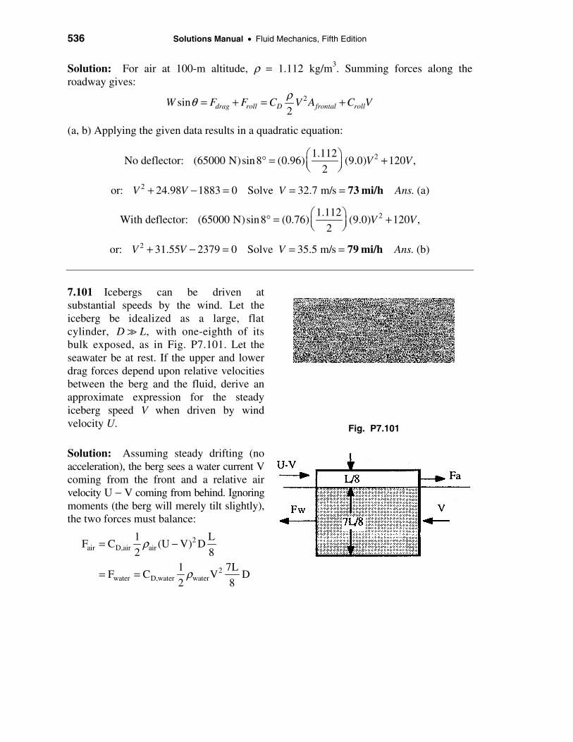
536 Solutions Manual • Fluid Mechanics, Fifth Edition
Solution: For air at 100-m altitude, ρ = 1.112 kg/m3. Summing forces along the roadway gives:
2sin2drag roll D frontal rollW F F C V A C Vρθ = + = +
(a, b) Applying the given data results in a quadratic equation:
21.112No deflector: (65000 N)sin8 (0.96) (9.0) 120 ,
2V V
° = +
2or: 24.98 1883 0 Solve 32.7 m/s (a)V V V Ans.+ − = = = 73 mi/h
21.112With deflector: (65000 N)sin8 (0.76) (9.0) 120 ,
2V V
° = +
2or: 31.55 2379 0 Solve 35.5 m/s (b)V V V Ans.+ − = = = 79 mi/h
7.101 Icebergs can be driven at substantial speeds by the wind. Let the iceberg be idealized as a large, flat cylinder, ,D L with one-eighth of its bulk exposed, as in Fig. P7.101. Let the seawater be at rest. If the upper and lower drag forces depend upon relative velocities between the berg and the fluid, derive an approximate expression for the steady iceberg speed V when driven by wind velocity U.
Solution: Assuming steady drifting (no acceleration), the berg sees a water current V coming from the front and a relative air velocity U − V coming from behind. Ignoring moments (the berg will merely tilt slightly), the two forces must balance:
2air D,air air
2water D,water water
1 LF C (U V) D
2 81 7L
F C V D2 8
ρ
ρ
= −
= =
Fig. P7.101

Chapter 7 • Flow Past Immersed Bodies 537
This has the form of a quadratic equation:
ραα αα ρ
α
−− + = = −
=
2 2 2 w Dw
berg winda Da
7 C1U 2UV V V , or V U where = 1
1 C
Since (5000), we approximate . bergV U/≈ α
7.102 Sand particles (SG = 2.7), approximately spherical with diameters from 100 to 250 µm, are introduced into an upward-flowing water stream. What is the minimum water velocity to carry all the particles upward?
Solution: Clearly the largest particles need the most water speed. Set net weight = drag:
3 2 2 2
2
4 ( 1)( ) , solve
6 2 4 3
4 mor: (9.81)(0.00025)(2.7 1)
3 s
wnet p w D
D
D
gD SGW g D C V D V
C
C V with V in
ρπ πρ ρ −= − = =
= − = 0.00555
Iterate in Figure 7.16b: ReD ≈ 10, CD ≈ 4, Vmin ≈ 0.04 m/s Ans.
7.103 When immersed in a uniform stream, a heavy rod hinged at A will hang at Pode’s angle θ, after L. Pode (1951). Assume the cylinder has normal drag coefficient CDn and tangential coefficient CDt, related to Vn and Vt, respectively. Derive an expression for θ as a function of system parameters. Compute θ for a steel rod, L = 40 cm, D = 1 cm, hanging in sea-level air at V = 35 m/s.
Solution: For sea-level air, take ρ = 1.225 kg/m3 and µ = 1.78E−5 kg/m⋅s. The tangential drag force passes right through A, so the moment balance is
Fig. P7.103
2 2A n Dn s
L L L LM F W cos C (V sin ) DL ( )g D L cos ,
2 2 2 2 4 2
Solve for Pode’s angle (a)Ans.
ρ πθ θ ρ ρ θ = − = − −
2s
2Dn
( )g( /2)Dsincos C V
ρ ρ πθθ ρ
−=

538 Solutions Manual • Fluid Mechanics, Fifth Edition
For the numerical data, take SG(steel) = 7.86, Ren ≈ 17000 (laminar), CDn ≈ 1.2: 2
2
sin [7.86(998) 1.225](9.81)( /2)(0.01)0.671, solve (b)
cos (1.225)(1.2)(35)Ans.
θ πθ
−= = θPode 44≈ °
*7.104 Suppose that the tractor-trailer truck of Prob. 7.100 is subjected to an un-powered, no-brakes, no-deflector coastdown on a sea-level road. The starting velocity is 65 mi/h. Solve, either analytically or on a computer, for the truck’s velocity V(t) and plot the results until the speed has dropped to 30 mi/h. What is the total coastdown time?
Solution: For air at 100-m altitude, ρ = 1.112 kg/m3. Summing forces along the roadway gives:
2
20
2
Separate the variables: , where2
final final
o
truck drag roll D frontal roll
V t
D frontalrV
dVm F F C V A C V
dt
m dVdt a C A
aV C V
ρ
ρ
= − − = − −
= − =+
After integration and rearrangement, the solution for deceleration time is:
ln where2
65000/9.81 29.06 4.804(13.41) 120For our data, 4.804 and ln
120 4.804(29.06) 120 13.41
final rofinal D frontal
r o r final
f
aV CVmt a C A
C aV C V
a t
ρ += = +
+ = = +
30 /: mi hor t Ans.≈ 23.8 s
We converted 65 and 30 mi/h to 29.06 and 13.41 m/s, respectively. A plot of the truck’s decelerating velocity is shown below.
Problem 7.104: Velocity vs. Time

Chapter 7 • Flow Past Immersed Bodies 539
7.105 A ship 50 m long, with a wetted area of 800 m2, has the hull shape of Fig. 7.19, with no bow or stern bulbs. Total propulsive power is 1 MW. For seawater at 20°C, plot the ship’s velocity V (in knots) versus power P for 0 < P < 1 MW. What is the most efficient setting?
Solution: For seawater at 20°C, take ρ = 1025 kg/m3 and µ = 0.00107 kg/m⋅s. The drag is taken to be the sum of friction and wave drag—which are defined differently:
2 2 2frict wave D,frict wet D,wave
1/7D,wave D,frict L
2 2 2Dfrict Dwave
F F F C V A C V L ,2 2
with C from Fig. 7.19 and C 0.031/Re (turbulent flat plate formula)
1025 1025 mHere, F C V (800) C V (50) , with V in m/s 1 1.94 kn
2 2 s
ρ ρ= + = +
≈
= + =
Assume different values of V, calculate friction and wave drag (the latter depending upon the Froude number V/√(gL) = V/√[9.81(50)] ≈ 0.0452V(m/s). Then compute the power in watts from P = FV, with F in newtons and V in m/s. Plot P versus V in knots on the graph below. The results show that, below 4 knots, wave drag is negligible and sharp increases in ship speed are possible with small increases in power. Wave drag limits the maximum speed to about 8 knots. There are two good high-velocity, “high slope” regions—at 6 knots and at 7.5 knots—where speed increases substantially with power.
7.106 A smooth steel ball 1-cm in diameter (W ≈ 0.04 N) is fired vertically at sea level at an initial velocity of 1000 m/s. Its drag coefficient is given by Fig. 7.20. Assuming a constant speed of sound (343 m/s), compute the maximum altitude attained (a) by a simple analytical estimate; and (b) by a computer program.

540 Solutions Manual • Fluid Mechanics, Fifth Edition
Solution: For sea-level air, take ρ = 1.225 kg/m3 and µ = 1.78E−5 kg/m⋅s. The initial Mach number is Mao = 1000/343 ≈ 2.9, so we are well out into the region in Fig. 7.20 where CD(sphere) ≈ 1.0 ≈ constant. The equation of motion is
2
2 2 2Dz D
d d C DF m W C V D , or g V
dt 2 4 dt 8m
ρ π πρ = = − − = − −
V V (1)
With m ≈ 0.0041 kg and Vo = 1000 m/s, we compute (dV/dt)t=0 ≈ 12000 m/s2! Hence the (high-drag) ball slows down pretty fast and does not go very high. An approximate analysis, assuming constant drag coefficient, is mathematically the same as in Prob. 7.98:
1 2of f D
f f
2f
1 1o f
V gV V tan tan t , where V 2W/ C ( /4)D
V V
For our data, V 2(0.04)/1.225(1.0)( /4)(0.01) 28.84 m/s
Also, tan (V /V ) tan (1000/28.84) 1.542 radians
ρ π
π
−
− −
= − =
= ≈
= ≈
Maximum altitude occurs when V = 0, or t = (28.84)(1.542)/(9.81) ≈ 4.53 s. The maximum altitude formula is also given in Prob. 7.98:
2 2o
max 2D f
max
Vm 0.0041 kg 1000z ln 1 ln 1
C A V 28.841.225(1.0)( /4)(0.01)
z (a)Ans.
ρ π
= + = +
≈ 300 m
(b) For a digital computer solution, we let drag coefficient vary with Mach number as in Fig. 7.20 and also let air density and viscosity vary. Equation (1) of this problem is integrated numerically, by Runge-Kutta or whatever. The results are plotted below:
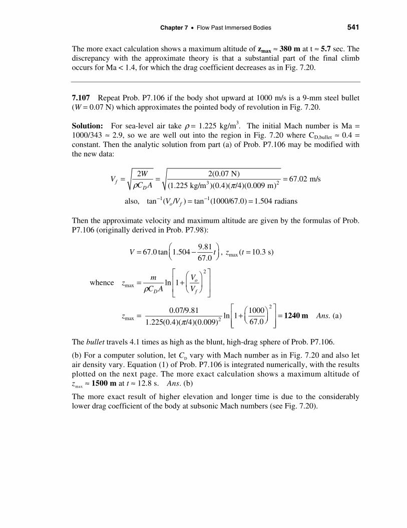
Chapter 7 • Flow Past Immersed Bodies 541
The more exact calculation shows a maximum altitude of zmax ≈ 380 m at t ≈ 5.7 sec. The discrepancy with the approximate theory is that a substantial part of the final climb occurs for Ma < 1.4, for which the drag coefficient decreases as in Fig. 7.20.
7.107 Repeat Prob. P7.106 if the body shot upward at 1000 m/s is a 9-mm steel bullet (W = 0.07 N) which approximates the pointed body of revolution in Fig. 7.20.
Solution: For sea-level air take ρ = 1.225 kg/m3. The initial Mach number is Ma = 1000/343 ≈ 2.9, so we are well out into the region in Fig. 7.20 where CD,bullet ≈ 0.4 = constant. Then the analytic solution from part (a) of Prob. P7.106 may be modified with the new data:
3 2
1 1
2 2(0.07 N)67.02 m/s
(1.225 kg/m )(0.4)( /4)(0.009 m)
also, tan ( / ) tan (1000/67.0) 1.504 radians
fD
o f
WV
C A
V V
ρ π− −
= = =
= =
Then the approximate velocity and maximum altitude are given by the formulas of Prob. P7.106 (originally derived in Prob. P7.98):
max
2
max
2
max 2
9.8167.0 tan 1.504 , ( 10.3 s)
67.0
whence ln 1
0.07/9.81 1000ln 1 . (a)
67.01.225(0.4)( /4)(0.009)
o
D f
V t z t
Vmz
C A V
z Ans
ρ
π
= − =
= +
= + = 1240 m
The bullet travels 4.1 times as high as the blunt, high-drag sphere of Prob. P7.106.
(b) For a computer solution, let CD vary with Mach number as in Fig. 7.20 and also let air density vary. Equation (1) of Prob. P7.106 is integrated numerically, with the results plotted on the next page. The more exact calculation shows a maximum altitude of zmax ≈ 1500 m at t ≈ 12.8 s. Ans. (b)
The more exact result of higher elevation and longer time is due to the considerably lower drag coefficient of the body at subsonic Mach numbers (see Fig. 7.20).

542 Solutions Manual • Fluid Mechanics, Fifth Edition
7.108 The data in Fig. P7.108 are for lift and drag of a spinning sphere from Ref. 12, pp. 7–20. Suppose a tennis ball (W ≈ 0.56 N, D ≈ 6.35 cm) is struck at sea level with initial velocity Vo = 30 m/s, with “topspin” (front of the ball rotating downward) of 120 rev/sec. If the initial height of the ball is 1.5 m, estimate the horizontal distance travelled before it strikes the ground.
Fig. P7.108

Chapter 7 • Flow Past Immersed Bodies 543
Solution: For sea-level air, take ρ = 1.225 kg/m3 and µ = 1.78E−5 kg/m⋅s. For this short distance, the ball travels in nearly a circular arc, as shown at right. From Figure P7.108 we read drag and lift:
D L
rad120(2 ) 754 ,
sR 754(0.03175)
0.80,V 30
Read C , C
ω π
ω
= =
= ≈
≈ ≈0.47 0.12
Initially, the accelerations in the horizontal and vertical directions are (z up, x to left)
2 2
x,0
2 2
z,0
drag 0.47(1.225/2)(30) ( /4)(0.0635)a
m 0.56/9.81
lift 0.12(1.225/2)(30) ( /4)(0.0635)a g 9.81
m 0.56/9.81
π
π
= − = − ≈
= − − = − − ≈
−
−
2
2
14.4 m/s
13.5 m/s
The term ax serves to slow down the ball from 30 m/s, when hit, to about 24 m/s when it strikes the floor about 0.5 s later. The average velocity is (30 + 24)/2 = 27 m/s. The term az causes the ball to curve in its path, so one can estimate the radius of curvature and the angle of turn for which ∆z = 1.5 m. Then, finally, one estimates ∆x as desired:
2 2avg 1
zV (27) 54 1.5
a , or: R 54 m; cos 13.54R 13.5 54
θ − − = ≈ ≈ = ≈ °
ballFinally, x Rsin (54)sin(13.54 ) Ans.θ∆ = = ° ≈ 12.6 m
A more exact numerical integration of the equations of motion (not shown here) yields the result ∆x ≈ 13.0 m at t ≈ 0.49 s.
7.109 Repeat Prob. 7.108 above if the ball is instead struck with “underspin,” that is, with the front of the ball rotating upward.
Solution: For sea-level air, take ρ = 1.225 kg/m3 and µ = 1.78E−5 kg/m⋅s. Again, for this short distance, the ball travels in nearly a circular arc, as shown above. This time the

544 Solutions Manual • Fluid Mechanics, Fifth Edition
lift acts against gravity, so the balls travels further with approximately the same ax. We find the new az and make the same “circular-arc” analysis to find Rnew, θ, and ∆xunderspin:
2 2
x,0 z,02
21
avg
m 0.12(1.225/2)(30) ( /4)(0.0635)a 14.4 , a 9.81
0.56/9.81s
m (27) 119 1.5V 27 , R 119 m; cos 9.12
s 6.14 119
π
θ −
= − = − + ≈
− ≈ = ≈ = ≈ °
− 2
m6.14
s
underspinFinally, x (119)sin(9.12 ) Ans.∆ = ° ≈ 18.8 m
7.110 A baseball pitcher throws a curveball with an initial velocity of 65 mi/h and a spin of 6500 r/min about a vertical axis. A baseball weighs 0.32 lbf and has a diameter of 2.9 in. Using the data of Fig. P7.108 for turbulent flow, estimate how far such a curveball will have deviated from its straightline path when it reaches home plate 60.5 ft away.
Solution: For sea-level air, take ρ = 0.00238 slug/ft3 and µ = 3.72E−7 slug/ft⋅s. Again, for this short distance, the ball travels
Fig. P7.110
in nearly a circular arc, as shown above. However, gravity is not involved in this curved horizontal path. First evaluate the lift and drag:
omi ft 2 rad R 681(2.9/24)
V 65 95 , 6500 681 , 0.86h s 60 s V 95
π ωω = = = = = ≈
D LFig. P7.108: Read C , C≈ ≈0.44 0.17
The initial accelerations in the x- and y-directions are
2 2
x,0
2 2
y,0
drag 0.44(0.00238/2)(95) ( /4)(2.9/12)a
m 0.32/32.2 slug
lift 0.17(0.00238/2)(95) ( /4)(2.9/12)a
m 0.32/32.2
π
π
= − = − ≈
= − = − ≈
2
2
ft22.0
s
ft8.5
s
−
−

Chapter 7 • Flow Past Immersed Bodies 545
The ball is in flight about 0.5 sec, so ax causes it to slow down to about 85 ft/s, with an average velocity of (95 + 85)/2 ≈ 90 ft/s. Then one can use these numbers to estimate R:
2 2avg 1 1
y
home plate
V (90) x 60.5R 954 ft; sin sin 3.63
|a | 8.5 R 954
Finally, y R(1 cos ) 954(1 cos3.63 ) Ans.
θ
θ
− −∆ = = ≈ = = ≈ °
∆ = − = − ° ≈ 1.9 ft
7.111 A table tennis ball has a mass of 2.6 g and a diameter of 3.81 cm. It is struck horizontally at an initial velocity of 20 m/s while it is 50 cm above the table, as in Fig. P7.111. For sea-level air, what topspin (as shown), in r/min, will cause the ball to strike the opposite edge of the table, 4 m away? Make an analytical estimate, using Fig. P7.108, and account for the fact that the ball decelerates during flight.
Fig. P7.111
NOTE: The table length is 4 meters.
Solution: For sea-level air, take ρ = 1.225 kg/m3 and µ = 1.78E−5 kg/m⋅s. This problem is difficult because the ball is so light and will decelerate greatly during its trip across the table. For the last time, as in Prob. 7.108, for this short distance, we assume the ball travels in nearly a circular arc, as analyzed there. First, from the geometry of the table, ∆x = 4 m, ∆z = 0.5 m, the required radius of curvature is known:
R(1 cos ) 0.5 m; R sin 4 m; solve for R m, 16.25 14.25θ θ θ− = = = = °
Then the centripetal acceleration should be estimated from R and the average velocity during the flight. Estimate, from Fig. P7.108, that CD ≈ 0.5. Then compute
2 2
2
0.5(1.225/2)(20) ( /4)(0.0381) m53
0.0026 sx,o
draga
mass
π= − = − = −

546 Solutions Manual • Fluid Mechanics, Fifth Edition
This reduces the ball speed from 20 m/s to about 12 m/s during the 0.25-s flight. Taking our average velocity as (20 + 12)/2 ≈ 16 m/s, we compute the vertical acceleration:
2 2 2 2
, 2
(16) m (1.225/2)(16) ( /4)(0.0381)15.75 9.81
16.25 0.0026savg L
z avg
V Ca
R
π= = = = +
,Solve for L avgC ≈ 0.086
From Fig. P7.108, this value of CL (probably laminar) occurs at about ωR/V ≈ 0.6, or ω = 0.6(16)/(0.0381/2) ≈ 500 rad/s ≈ 4800 rev/min. Ans.
7.112 A smooth wooden sphere (SG = 0.65) is connected by a thin rigid rod to a hinge in a wind tunnel, as in Fig. P7.112. Air at 20°C and 1 atm flows and levitates the sphere. (a) Plot the angle θ versus sphere diameter d in the range 1 cm ≤ d ≤ 15 cm. (b) Comment on the feasibility of this configuration. Neglect rod drag and weight.
Fig. P7.112
Solution: For air, take ρ = 1.2 kg/m3 and µ = 1.8E−5 kg/m⋅s. If rod drag is neglected and L d, the balance of moments around the hinge gives:
3
2 2
3
2 2
( /6)0 sin cos , tan
( /2) ( /4)
(0.65)(998)(9.81)( /6): tan 49.1 .
(1.2/2) (12) ( /4)
whinge
a D
DD
g dWM FL WL or
F C V d
d dInput the data with d in meters
CC d
ρ πθ θ θρ π
πθπ
= = − = =
= =
We find CD from Red = ρVd/µ = (1.2)(12)d/(0.000018) = 8E5d (with d in meters). For d = 1 cm, Red = 8000, Fig. 7.16b, CD = 0.5, tanθ = 0.982, θ = 44.5°. At the other extreme, for d = 15 cm, Red = 120000, Fig. 7.16b, CD = 0.5, tanθ = 14.73, θ = 86.1°.
(a) A complete plot is shown at right. (b) This is a ridiculous device for either velocity or diameter.
00 0.05 0.1 0.15
20
40
60
80
100
Problem 7.112: Angles vs. Diameter

Chapter 7 • Flow Past Immersed Bodies 547
7.113 An auto has m = 1000 kg and a drag-area CDA = 0.7 m2, plus constant 70-N rolling resistance. The car coasts without brakes at 90 km/h climbing a hill of 10 percent grade (5.71°). How far up the hill will the car come to a stop?
Fig. P7.113
Solution: For sea-level air, take ρ = 1.225 kg/m3 and µ = 1.78E−5 kg/m⋅s. If x denotes uphill, the equation of motion is
2rolling D
–1 o r rf f
f f D
dVm Wsin – F – C A V , separate the variables and integrate:
dt 2
V W sin F Wsin FV V tan tan – t , where V
V mV C A / 2
ρθ
θ θρ
= −
+ += =
For the particular data of this problem, we evaluate
rf
f
–1
9810sin 5.71° 70 m Wsin F 9810sin 5.71° 70V 49.4 , 0.0212
0.7(1.225/2) s mV 1000(49.4)
25also tan 0.469 radians. So, finally, V 49.4 tan[0.469 – 0.0212t]
49.4
θ+ + += ≈ = ≈
= ≈
The car stops at V = 0, or tfinal = 0.469/0.0212 ≈ 22.1 s. The distance to stop is computed by the same formula as in Prob. 7.98:
2 2o
maxD f
Vm 1000 25x ln 1 ln 1
C A V 1.225(0.7) 49.4Ans.
ρ
∆ = + = + ≈
266 m
7.114 Suppose the car in Prob. 7.113 above is placed at the top of the hill and released from rest to coast down without brakes. What will be the car speed, in km/h, after dropping a vertical distance of 20 m?
Solution: Here the car weight assists the motion, and, if x is downhill,
2r D
r Drf f
D
dVm Wsin F – C A V , separate the variables and integrate to get
dt 2
(Wsin F )C A /22(Wsin F )V = V tanh(Ct), where V and C =
C A m
ρθ
θ ρθρ
= −
−−=

548 Solutions Manual • Fluid Mechanics, Fifth Edition
For our particular data, evaluate
f
1
2(9810sin 5.71° 70) mV 46.0 ;
1.225(0.7) s
(9810sin 5.71° 70)(0.7)(1.225/2)C 0.0197 s
1000−
−= =
−= =
We need to know when the car reaches ∆x = (20 m)/sin(5.71°) ≈ 201 m. The above expression for V(t) may be readily integrated:
tf
0
V 46.0x V dt ln[ cosh(Ct)] ln[ cosh(0.0197t)] 201 m if t
C 0.0197
Then, at x 201 m, z 20 m, 46.0 tanh[0.0197(21.4)] Ans.
∆ = = = = ≈
∆ = ∆ = = ≈
21.4 s
m kmV 18.3 65.9
s h=
7.115 The Cessna Citation executive jet weighs 67 kN and has a wing area of 32 m2. It cruises at 10 km standard altitude with a lift coefficient of 0.21 and a drag coefficient of 0.015. Estimate (a) the cruise speed in mi/h; and (b) the horsepower required to maintain cruise velocity.
Solution: At 10 km standard altitude (Table A-6) the air density is 0.4125 kg/m3. (a) The cruise speed is found by setting lift equal to weight:
32 2 20.4125 kg/m
67000 N 0.21 (32 m ),2 2
mSolve 220 (a)
s
L wingLift C V A V
V Ans.
ρ = = =
= = mi492
h
(b) With speed known, the power is found from the drag:
2 20.41250.015 (220) (32) (220)
2 2
1.05 MW (b)
drag DPower F V C V A V
Ans.
ρ = = =
= = 1410 hp
7.116 An airplane weighs 180 kN and has a wing area of 160 m2 and a mean chord of 4 m. The airfoil properties are given by Fig. 7.25. If the plane is designed to land at Vo = 1.2Vstall, using a split flap set at 60°, (a) What is the proper landing speed in mi/h? (b) What power is required for takeoff at the same speed?

Chapter 7 • Flow Past Immersed Bodies 549
Solution: For air at sea level, ρ ≈ 1.225 kg/m3. From Fig. 7.24 with the flap, CL,max ≈ 1.75 at α ≈ 6°. Compute the stall velocity:
3 2max
,max2 2
2 2(180000 N) m32.4
s(1.225 kg/m )(1.75)(160 m )
Then 1.2 . (a)
1.751.22
( ) (1.2)
stallL, p
landing stall
LL
land stall
WV
C A
V V Ans
CC
V /V
ρ= = =
= =
= = =
m38.9
s
For take-off at the same speed of 38.9 m/s, we need a drag estimate. From Fig. 7.25 with a split flap, CD∞ ≈ 0.04. We don’t have a theory for induced drag with a split flap, so we just go along with the usual finite wing theory, Eq. (7.71). The aspect ratio is b/c = (40 m)/(4 m) =10.
2 2
2
(1.22)0.04 0.087,
(10)
1.225(0.087) (38.9) (160) 12900 N
2
LD D
drag
CC C
AR
F
π π∞= + = + =
= =
Power required = FV = (12900 N)(38.9 m/s) = 501000 W = 672 hp Ans. (b)
7.117 Suppose the airplane of Prob. 7.116 takes off at sea level without benefit of flaps and with constant lift coefficient and take-off speed of 100 mi/h. (a) Estimate the take-off distance if the thrust is 10 kN. (b) How much thrust is needed to make the take-off distance 1250 m?
Solution: For air at sea level, ρ = 1.225 kg/m3. Convert V = 100 mi/h = 44.7 m/s. From Fig. 7.25, with no flap, read CD∞ ≈ 0.006. Compute the lift and drag coefficients:
2 3 2 2
2 2
2 2(180000 N)0.919 (assumed constant)
(1.225 kg/m )(44.7 m/s) (160 m )
(0.919)0.006 0.0329
(10)
Lp
LD D
WC
V A
CC C
AR
ρ
π π∞
= = =
= + = + =
The take-off drag is Do = CD(ρ/2)V2Ap = (0.0329)(1.225/2)(44.7)2(160) = 6440 N. From Ex. 7.8,
ln , ( /2) (0.0329)(1.225/2)(160) 3.22 kg/m2
(180000/9.81) kg 10000 NThen ln . (a)
2(3.22 kg/m) 10000 N 6440 N
o D po
o
m TS K C A
K T D
S Ans
ρ
= = = = −
= = −2940 m

550 Solutions Manual • Fluid Mechanics, Fifth Edition
(b) To decrease this take-off distance to 1250 m, we need more thrust, computed as follows:
(180000/9.81) kg1250 m ln , Solve . (b)
2(3.22 kg/m) 6440 NoT
S AnsT
= = −T 18100 N≈
7.118 Suppose the airplane of Prob. 7.116 is now fitted with all the best high-lift devices of Fig. 7.28. (a) What is its minimum stall speed in mi/h? (b) Estimate the stopping distance if the plane lands at Vo = 1.25Vstall with constant CL = 3.0 and CD = 0.2 and the braking force is 20% of the weight on the wheels.
Solution: For air at sea level, ρ = 1.225 kg/m3. From Fig. 7.28 read CL,highest ≈ 4.0.
3 2,max
2 2(180000 N) m(a) Then 21 4
s(1.225 kg/m )(4.0)(160 m )
mThus 1.25 26.8 . (a)
s
stallL p
land stall
WV .
C A
V V Ans
ρ= = =
= = ≈ mi60
h
(b) With constant lift and drag coefficients, we can set up and solve the equation of motion:
2 0.2( )2x drag brake D p
dVF m F F C V A Weight Lift
dt
ρ = = − − = − − −
2 2
2
180000 1.225 1.225or: 0.2 (160) 0.2 180000 3.0 (160)
9.81 2 2
Clean this up: 0.00214 1.962
dVV V
dt
dVV
dt
= − − −
= + −
We could integrate this twice and calculate V = 0 (stopping) at t = 21.5 s and Smax = 360 m. Or, since we are looking for distance, we could convert dV/dt = (1/2)d (V2)/ds to obtain
max
2
02 22
20
max 2
1 ( )0.00214 1.962, or: 2
2 0.00214 1.962
1 1.962Solution: ln . (b)
2(0.00214) 1.962 0.00214(26.8)
o
S
V
dV dV d VV ds
dt ds V
S Ans
= = − =−
= ≈ −
360 m

Chapter 7 • Flow Past Immersed Bodies 551
7.119 An airplane has a mass of 5000 kg, a maximum thrust of 7000 N, and a rectangular wing with aspect ratio 6.0. It takes off at sea level with a 60° split flap as in Fig. 7.25. Assume all lift and drag are due to the wing. What is the proper wing size if the take-off distance is to be 1 km?
Solution: Once again take sea-level density of ρ ≈ 1.225 kg/m3. With the wing size unknown, practically nothing can be calculated in advance. However, from Fig. 7.25 with the 60° flap, we note that CL,max ≈ 1.75 and CD∞ ≈ 0.04. The rest can at least be listed:
2o o D o o stall
D o L,max
m T 2 WS ln , where D C bcV , V 1.2V 1.2
C A T D 2 C bc
band we know that AR 6.0, W 5000(9.81) N, T 7000 N.
c
ρρ ρ
= = ≈ = −
= = = =
We also know (crudely), that CD ≈ CD∞ + CL2/(πAR). Since CL = 1.75/(1.2)2 = 1.22, we
know the drag coefficient, CD ≈ 0.04 + (1.22)2/[6π] ≈ 0.118. Our approach is simply to assume a chord and iterate until the proper take-off distance, So = 1000 m, is obtained:
Guess c = 2.0 m, b = 12.0 m, then Vo = 52.4 m/s, Do = 4777 N, So = 1648 m
try c = 3.0 m, b = 18.0 m, so Vo = 34.9 m/s, Do = 4777 N, So = 733 m
This process converges to So = 1000 m at c = 2.57 m, b = 15.4 m Ans.
Instead of iteration, someone cleverer than I might notice, in advance, that the take-off drag is independent of the wing size, since it is related to the stall speed:
2 Do D o D
L,max L,max
o 2D o
2 W CD C bcV C bc 1.44 1.44 W 4777 N
2 2 C bc C
m T 5000 7000Thus S 1000 m ln ln ,
C A T D 7000 47771.225(0.118)6c
or
ρ ρρ
ρ
= = = =
= = = − −
c 2.57 m=
7.120 Show that, if Eqs. (7.70) and (7.71) are valid, the maximum lift-to-drag ratio occurs when CD = 2CD∞. What are (L/D)max and α for a symmetric wing when AR = 5.0 and CD∞ = 0.009?

552 Solutions Manual • Fluid Mechanics, Fifth Edition
Solution: According to our lift and induced-drag approximations, Eqs. (7.70) and (7.71), the lift-to-drag ratio is
L L2
D LD L
L C C d L; Differentiate: 0 if
D C dC DC C /( AR)Ans.
π∞
= = = + D DC 2C ∞=
For our numerical example, compute, at maximum L/D,
L D D DAR 5, C C AR (0.009) (5) 0.376, C 2C 0.018π π∞ ∞= = = ≈ = =
Therefore, L/D|max = 0.376/0.018 ≈ 21 Ans.
Also, CL = 0.376 = 2π sin α/[1 + 2/AR] = 2π sin α/[1 + 2/5], solve α ≈ 4.8° Ans.
7.121 In gliding (unpowered) flight, lift and drag are in equilibrium with the weight. Show, that, with no wind, the craft sinks at an angle tanθ ≈ drag/lift. For a sailplane with m = 200 kg, wing area = 12 m2, AR = 12, with an NACA 0009 airfoil, estimate (a) stall speed, (b) minimum gliding angle; (c) the maximum distance it can glide in still air at z = 1200 m.
Lift
Drag
Weight
Horizontal
V
θ
θ
Fig. P7.121
Solution: By the geometry of the figure, with no thrust, wind, or acceleration,
L DW , or:
cos sinAns.
θ θ= = glide
Dtan
L= θ
The NACA 0009 airfoil is shown in Fig. 7.25, with CD∞ ≈ 0.006. From Table A-6, at z = 1200 m, ρ ≈ 1.09 kg/m3. Then, as in part (b) of Prob. 7.120 above,
L D maxL L 0.476
at max , C C AR 0.006 (12) 0.476, 39.6D D 2(0.006)
π π∞= = = = ≈|
Thus tanθmin = 1/39.6 or θmin ≈ 1.45° Ans. (b)
Meanwhile, from Fig. 7.25, CL,max ≈ 1.3, so the stall speed at 1200 m altitude is
stallL,max
2 W 2(200)(9.81)V (a)
C A 1.09(1.3)(12)Ans.
ρ= = ≈ m
15.2s
With θmin = 1.45° and z = 1200 m, the craft can glide 1200/tan(1.45°) ≈ 47 km Ans. (c).

Chapter 7 • Flow Past Immersed Bodies 553
7.122 A boat of mass 2500 kg has two hydrofoils, each of chord 30 cm and span 1.5 meters, with CL,max = 1.2 and CD∞ = 0.08. Its engine can deliver 130 kW to the water. For seawater at 20°C, estimate (a) the minimum speed for which the foils support the boat, and (b) the maximum speed attainable.
Solution: For seawater at 20°C, take ρ = 1025 kg/m3 and µ = 0.00107 kg/m⋅s. With two foils, total planform area is 2(0.3 m)(1.5 m) = 0.9 m2. Thus the stall speed is
L,max
2W 2(2500)(9.81) (a)
C A 1025(1.2)(0.9)Ans.
ρ= = ≈min
mV 6.66 (13 knots)
s≈
Given AR = 1.5/0.3 = 5.0. At any speed during lifting operation (V > Vmin), the lift and drag coefficients, from Eqs. (7.70) and (7.71), are
L 2 2 2
2 2 2L
D D 4
2W 2(2500)(9.81) 53.2C ;
AV 1025(0.9)V V
C (53.2/V ) 180.0C C 0.08 0.08
AR (5.0) V
ρ
π π∞
= = =
= + = + = +
24
4
180 1025Power DV 0.08 V (0.9)V 130 hp 745.7 96900 W
2V
Clean up and rearrange: V 2627V 2250 0,
Solve (b)Ans.
= = + = × =
− + =
maxm
V 13.5 26 kns
≈ ≈
Three other roots: 2 imaginary and V4 = 0.86 m/s (impossible, below stall)
7.123 In prewar days there was a controversy, perhaps apocryphal, about whether the bumblebee has a legitimate aerodynamic right to fly. The average bumblebee (Bombus terrestris) weighs 0.88 g, with a wing span of 1.73 cm and a wing area of 1.26 cm2. It can indeed fly at 10 m/s. Using fixed-wing theory, what is the lift coefficient of the bee at this speed? Is this reasonable for typical airfoils?
Solution: Assume sea-level air, ρ = 1.225 kg/m3. Assume that the bee’s wing is a low-aspect-ratio airfoil and use Eqs. (7.68) and (7.72):
2 2
L2 2 2p p
b (1.73 cm) 2W 2(0.88E 3)(9.81)AR ; C
A 1.26 cm V A 1.225(10) (1.26E 4)2.38
ρ−= = = = = ≈
−1.12
This looks unreasonable, CL → CL,max and the bee could not fly slower than 10 m/s.

554 Solutions Manual • Fluid Mechanics, Fifth Edition
Even if this high lift coefficient were possible, the angle of attack would be unrealistic:
L stall
? 2 sinC 1.12 , with AR 2.38, solve for (too high, > )
1 2/AR
π α α α= = = ≈+
19°
7.124 The bumblebee can hover at zero speed by flapping its wings. Using the data of Prob. 7.123, devise a theory for flapping wings where the downstroke approximates a short flat plate normal to the flow (Table 7.3)
width “b”
R
drr
θθ
Ω
and the upstroke is feathered at nearly zero drag. How many flaps per second of such a model wing are needed to support the bee’s weight? (Actual measurements of bees show a flapping rate of 194 Hz.)
Solution: Any “theory” one comes up with might be crude. As shown in the figure, let the wings flap sinusoidally, between ±θo, that is, θ = θo cos Ωt. Let the upstroke be feathered (zero force), and let the downstroke be strong enough to create a total upward force of 0.75 W on each wing—to compensate for zero lift during upstroke. Assume a short flat plate (Table 7.3), CD ≈ 1.2. Then, on each strip dr of wing, the elemental drag force is
2D o
R2 2 2 3 2
D o D o avg0
ddF C V bdr, where V r r sin( t)
2 dt
F C (r sin t) b dr C bR [sin t] 0.75 W2 6
ρ θ θ
ρ ρθ θ
= = = Ω Ω
= Ω Ω = Ω Ω ≈
2o avg
1Assume full flapping: and [sin t]
2 2
πθ = Ω ≈
22 31.225
Evaluate F 0.75(0.00088)(9.81) (1.2) (0.00728)(0.00865)12 2
π = ≈ Ω
Solve for 2132 rad/s 2 / Ans.πΩ ≈ ÷ ≈ 340 rev s
This is about 75% higher than the measured value Ωbee ≈ 194 Hz, but it’s a crude theory!
7.125 In 2001, a commercial aircraft lost all power while flying at 33,000 ft over the open Atlantic Ocean, about 60 miles from the Azores Islands. The pilots, with admirable skill, put the plane into a shallow glide and successfully landed in the Azores. Assume

Chapter 7 • Flow Past Immersed Bodies 555
that the airplane satisfies Eqs. (7.70) and (7.71), with AR = 7, Cd∞ = 0.02, and a symmetric airfoil. Estimate its optimum glide distance with a mathematically perfect pilot.
Solution: From Problem P7.120, the maximum lift-to-drag ratio occurs when Cd = 2Cd∞ = 2(0.02) = 0.04 in the present case. Accordingly, for maximum L/D ratio, the lift coefficient is CL = [Cd∞πAR]1/2 = [0.02π (7)]1/2 = 0.663. From Prob. 7.121, the glide angle of an unpowered aircraft is such that tanθ = drag/lift = Cd /CL. Thus, the pilots’ optimum glide is:
min0.04 1 33000 ft
tan ,0.663 16.6
547000 ftor
Drag
Lift Glide distance
Ans.
θ = = = =
= ≈
|min
104 milesGlide

556 Solutions Manual • Fluid Mechanics, Fifth Edition
FUNDAMENTALS OF ENGINEERING EXAM PROBLEMS: Answers
FE7.1 A smooth 12-cm-diameter sphere is immersed in a stream of 20°C water moving at 6 m/s. The appropriate Reynolds number of this sphere is
(a) 2.3E5 (b) 7.2E5 (c) 2.3E6 (d) 7.2E6 (e) 7.2E7
FE7.2 If, in Prob. FE7.1, the drag coefficient based on frontal area is 0.5, what is the drag force on the sphere?
(a) 17 N (b) 51 N (c) 102 N (d) 130 N (e) 203 N
FE7.3 If, in Prob. FE7.1, the drag coefficient based on frontal area is 0.5, at what terminal velocity will an aluminum sphere (SG = 2.7) fall in still water?
(a) 2.3 m/s (b) 2.9 m/s (c) 4.6 m/s (d) 6.5 m/s (e) 8.2 m/s
FE7.4 For flow of sea-level standard air at 4 m/s parallel to a thin flat plate, estimate the boundary-layer thickness at x = 60 cm from the leading edge:
(a) 1.0 mm (b) 2.6 mm (c) 5.3 mm (d) 7.5 mm (e) 20.2 mm
FE7.5 In Prob. FE7.4, for the same flow conditions, what is the wall shear stress at x = 60 cm from the leading edge?
(a) 0.053 Pa (b) 0.11 Pa (c) 0.016 Pa (d) 0.32 Pa (e) 0.64 Pa
FE7.6 Wind at 20°C and 1 atm blows at 75 km/h past a flagpole 18 m high and 20 cm in diameter. The drag coefficient based upon frontal area is 1.15. Estimate the wind-induced bending moment at the base of the pole.
(a) 9.7 kN⋅m (b) 15.2 kN⋅m (c) 19.4 kN⋅m (d) 30.5 kN⋅m (e) 61.0 kN⋅m
FE7.7 Consider wind at 20°C and 1 atm blowing past a chimney 30 m high and 80 cm in diameter. If the chimney may fracture at a base bending moment of 486 kN⋅m, and its drag coefficient based upon frontal area is 0.5, what is the approximate maximum allowable wind velocity to avoid fracture?
(a) 50 mi/h (b) 75 mi/h (c) 100 mi/h (d) 125 mi/h (e) 150 mi/h
FE7.8 A dust particle of density 2600 kg/m3, small enough to satisfy Stokes drag law, settles at 1.5 mm/s in air at 20°C and 1 atm. What is its approximate diameter?
(a) 1.8 µm (b) 2.9 µm (c) 4.4 µm (d) 16.8 µm (e) 234 µm
FE7.9 An airplane has a mass of 19,550 kg, a wing span of 20 m, and an average wind chord of 3 m. When flying in air of density 0.5 kg/m3, its engines provide a thrust of 12 kN against an overall drag coefficient of 0.025. What is its approximate velocity?
(a) 250 mi/h (b) 300 mi/h (c) 350 mi/h (d) 400 mi/h e) 450 mi/h
FE7.10 For the flight conditions of the airplane in Prob. FE7.9 above, what is its approximate lift coefficient?
(a) 0.1 (b) 0.2 (c) 0.3 (d) 0.4 (e) 0.5

Chapter 7 • Flow Past Immersed Bodies 557
COMPREHENSIVE PROBLEMS
C7.1 Jane wants to estimate the drag coefficient of herself on her bicycle. She measures the projected frontal area to be 0.40 m2 and the rolling resistance to be 0.80 N⋅s/m. Jane coasts down a hill with a constant 4° slope. The bike mass is 15 kg, Jane’s mass is 80 kg. She reaches a terminal speed of 14 m/s down the hill. Estimate the aerodynamic drag coefficient CD of the rider and bicycle combination.
Solution: For air take ρ ≈ 1.2 kg/m3. Let x be down the hill. Then a force balance is
2
0 sin ,
where ,2
x drag rolling
drag D rolling RR
F mg F F
F C V A F C V
φρ
= = − −
= =
Solve for, and evaluate, the drag coefficient:
2 2
sin 95(9.81)sin 4 0.8(14)
(1/2) (1/2)(1.2)(14) (0.4)RR
Dmg C V
C Ans.V A
φρ
− ° −= = ≈ 1.14
Fig. C7.1
C7.2 Air at 20°C and 1 atm flows at Vavg = 5 m/s between long, smooth parallel heat-exchanger plates 10 cm apart, as shown below. It is proposed to add a number of widely spaced 1-cm-long thin ‘interrupter’ plates to increase the heat transfer, as shown. Although the channel flow is turbulent, the boundary layer over the interrupter plates is laminar. Assume all plates are 1 m wide into the paper. Find (a) the pressure drop in Pa/m without the small plates present. Then find (b) the number of small plates, per meter of channel length, which will cause the overall pressure drop to be 10 Pa/m.
Fig. C7.2

558 Solutions Manual • Fluid Mechanics, Fifth Edition
Solution: For air, take ρ = 1.2 kg/m3 and µ = 1.8E−5 kg/m⋅s. (a) For wide plates, the hydraulic diameter is Dh = 2h = 20 cm. The Reynolds number, friction factor, and pressure drop for the bare channel (no small plates) is:
,
2 2
(1.2)(5.0)(0.2)66,700 ( )
1.8 5
0.0196
1.0 m 1.2(0.0196) (5.0) (a)
2 0.2 m 2
avg hDh
Moody smooth
bare avgh
V DRe turbulent
E
f
Lp f V Ans.
D
ρµ
ρ
= = =−
≈
∆ = = =
Pa1.47
m
Each small plate (neglecting the wake effect if the plates are in line with each other) has a laminar Reynolds number:
,
2 21 2
(1.2)(5.0)(0.01)5 5,
1.8 5
1.328 1.3280.0230
3333
1.2 N(0.0230) (5.0) (2 0.01 1) 0.0069
2 2 plate
avg plateL
DL
plate D avg sides
V LRe E laminar
E
CRe
F C V A
ρµ
ρ
= = = < ∴−
= = ≈
= = × × =
3333
laminar
Each plate force must be supported by the channel walls. The effective pressure drop will be the bare wall pressure drop (assumed unchanged) plus the sum of the interrupter-plate forces divided by the channel cross-section area, which is given by (h × 1 m) = 0.1 m2. The extra pressure drop provided by the plates, for this problem, is (10.0 − 1.47) = 8.53 Pa/m. Therefore we need
21
8.53 Pa/m (b)
( / ) (0.0069 N/plate)/(0.1 m )needed
plate
pNo. of plates Ans.
F A
∆= = ≈ 124 plates
This is the number of small interrupter plates needed for each meter of channel length to build up the pressure drop to 10.0 Pa/m.
C7.3 A new pizza store needs a delivery car with a sign attached. The sign is 1.5 ft high and 5 ft long. The boss wants to mount the sign normal to the car’s motion. His employee, a student of fluid mechanics, suggests mounting it parallel to the motion. (a) Calculate the drag on the sign alone at 40 mi/h (58.7 ft/s) in both orientations. (b) The car has a rolling resistance of 40 lbf, a drag coefficient of 0.4, and a frontal area of 40 ft2. Calculate the total drag of the car-sign combination at 40 mi/h. (c) Include rolling resistance and calculate the horsepower required in both orientations. (d) If the engine

Chapter 7 • Flow Past Immersed Bodies 559
delivers 10 hp for 1 hour on a gallon of gasoline, calculate the fuel efficiency in mi/gal in both orientations, at 40 mi/h.
Solution: For air take ρ = 0.00237 slug/ft3. (a) Table 7.3, blunt plate, CD ≈ 1.2:
2 20.002371.2 (58.7) (1.5 5.0) (a— )
2 2normal DF C V A Ans. normalρ = = × ≈
37 lbf
For parallel orientation, take m = 3.76E−7 slug/ft⋅s. Use flat-plate theory for ReL = 0.00237(58.7)(5.0)/(3.76E−7) = 1.85E6 = transitional—use Eq. (7.49a):
1/7 1/7
0.031 1440 0.031 14400.00317
Re 1.85E6Re (1.85E6)D
LL
C = − = − ≈
20.002370.00317 (58.7) (1.5 5 2 ) (a— )
2parallelF sides Ans. parallel = × × ≈
0.19 lbf
(b) Add on the drag of the car:
2 2,
0.002370.4 (58.7) (40) 65.3 lbf
2 2car D car carF C V Aρ = = ≈
(1) sign ⊥: Total Drag = 65.3 + 36.7 ≈ 102 lbf Ans. (b—normal)
(2) sign //: Total Drag = 65.3 + 0.2 ≈ 65.5 lbf Ans. (b—parallel)
(c) Horsepower required = total force times velocity (include rolling resistance): (1) P⊥ = FV = (102 + 40)(58.7) = 8330 ft⋅lbs/s ÷ 550 ≈ 15.1 hp Ans. (c—normal) (2) P // = (65.5 + 40)(58.7) = 6190 ft⋅lbf/s ÷ 550 ≈ 11.3 hp Ans. (b—parallel)
(d) Fuel efficiency:
//
mi hp h 1(1) 40 10 (d— )
h gal 15.1 hp
mi hp h 1(2) 40 10 (d— )
h gal 11.3 hp
mpg Ans. normal
mpg Ans. parallel
⊥ ⋅ = ≈
⋅ = ≈
mi26.5
gal
mi35.4
gal
We see that the student is correct, there are fine 25% savings with the sign parallel.

560 Solutions Manual • Fluid Mechanics, Fifth Edition
C7.4 Consider a simple pendulum with an unusual bob shape: a cup of diameter D whose axis is in the plane of oscillation. Neglect the mass and drag of the rod L. (a) Set up the differential equation for θ (t) and (b) non-dimensionalize this equation. (c) Determine the natural frequency for
1.θ (d) For L = 1 m, D = 1 cm, m = 50 g, and air at 20°C and 1 atm, and θ (0) = 30°, find (numerically) the time required for the oscillation amplitude to drop to 1°.
Fig. C7.4
Solution: (a) Let Leq = L + D/2 be the effective length of the pendulum. Sum forces in the direction of the motion of the bob and rearrange into the basic 2nd-order equation:
2 2sin m , where2 4
ttangential D t t eq
dV dF mg C V D V L
dt dt
ρ π θθ = − − = =
2
Rearrange: , where (a)8 m
D eqC L DK Ans.
ρ π=
.. .θ θ θ+ + =
eq
gK
L2 sin 0
Note that CD ≈ 0.4 when moving to the right and about 1.4 moving to the left (Table 7.3).
(b) Now θ is already dimensionless, so define dimensionless time τ = t(g/Leq)1/2 and
substitute into the differential equation above. We obtain the dimensionless result
(b)Ans.
d dK
dd
22
2 0θ θ θ
ττ+ + =
Thus the only dimensionless parameter is K from part (a) above. (c) For 1,θ the term involving K is neglected, and sinθ ≈ θ itself. We obtain
..2 0, where (c)n Ans.θ ω θ+ ≈ ω n
eq
gL
=
Thus the natural frequency is (g/Leq)1/2 just as for the simple drag-free pendulum. Recall
that Leq = L + D/2. Note again that K has a different value when moving to the right (CD ≈ 0.4) or to the left (CD ≈ 1.4).
(d) For the given data, ρair = 1.2 kg/m3, Leq = L + D/2 = 1.05 m, and the parameter K is
2(1.2)(1.05) (0.1)0.099 0.0396 ( )
8(0.050)D
DC
K C moving to the rightπ= = =
0.1385 ( )moving to the left=

Chapter 7 • Flow Past Immersed Bodies 561
The differential equation from part (b) is then solved for θ (0) = 30° = π /6 radians. The natural frequency is (9.81/1.05)1/2 = 3.06 rad/s, with a dimensionless period of 2π. Integrate numerically, with Runge-Kutta or MatLab or Excel or whatever, until θ = 1° = π/180 radians. The time-series results are shown in the figure below.
We see that the pendulum is very lightly damped—drag forces are only about 1/50th of the weight of the bob. After ten cycles, the amplitude has only dropped to 22.7°—we will never get down to 1° in the lifetime of my computer. The dimensionless period is 6.36, or only 1% greater than the simple drag-free theoretical value of 2π.