CFD for Hydraulic Structures (535 kB) - NTNUfolk.ntnu.no/nilsol/cfd/cfdstr.pdf · CFD modelling for...

Department of Hydraulic and Environmental EngineeringThe Norwegian University of Science and Technology

CFD modelling for hydraulic structures

Nils Reidar B. Olsen

Preliminary 1st edition, 8. May 2001

ISBN 82-7598-048-8

CFD Modelling for Hydraulic Structures 2

Foreword

The present book is written as class notes for an advanced undergrad-uate course in hydraulic engineering at NTNU. The course will be given in the fifth and last year of the study. Previously, the students must have taken the fourth year course SIB 5050 Hydroinformatics for fluvial hy-draulics and limnology. This course gives the students basic knowledge and experience in CFD theory and use of CFD models. The present course builds on this knowledge, and expands further details on the spe-cifics of modelling hydraulic structures.

In the present text, the implementation of the algorithms are focused on the SSIIM model. This is partly because I am most familiar with this mod-el, and partly because this model will be used by my students. The al-ternative is to use a commercial CFD package, and this is presently too expensive.

The text sums up experiences we have had for several years with using SSIIM on modelling flow for hydraulic structures. I therefore I hope it can also be useful for external SSIIM users.

I want to thank all the people who have given me advice on modelling hydraulic structures over the years. Hilde Marie Kjellesvig must be men-tioned especially in this respect. I also want to thank her for permission to use her input data sets for the Himalayan Intake, in Chapter 5.5. Also thanks to Thorsten Stösser and Tim Fisher-Antze for using the figures and data for the Pasche case in Chapter 2.5.

3 Table of content

Table of content

Foreword 2

Table of content 3

1. Introduction 4

2. Vegetation 52.1 Roughness 52.2 Formulas 62.3 Implementation in SSIIM 72.4 Example 1. Sokna river 82.5 Example 2. Pasche channel 11

3. Spillways 133.1 Algorithms for free surface flow 133.2 Implementation in SSIIM 153.3 Example 1. Standard spillway 153.4 Example 2. Spillway with 3D contraction 173.5 Example 3. Shock waves 19

4. Local scour 214.1 Sediment transport modelling 214.2 Implementation in SSIIM 224.3 Example: Scour around a circular cylinder 22

5. Intakes 275.1 Intake layout and sediment problems 275.2 Modelling complex structures with SSIIM 275.3 Example 1. Sediment deposition in a sand trap 285.4 Example 2. Bed changes in a sand trap 295.5 Example 3. Complex geometries - Himalaya intake 32

Literature 35


1. Introduction

In recent years computers have become fast enough to make CFD com-putations feasible for engineering purposes. Some guidance is needed on how to model different types of hydraulic structures. In the present text, four types of problems are considered:

- Vegetation/stones in rivers- Spillways- Intakes- Local scour

Modelling flow in natural rivers using CFD is commonly used to make environmental assessment studies, for example habitat for fish, disper-sion of pollutants etc. This is a relatively straightforward procedure, giv-en todays CFD models. However, two types of problems often occur:

- The river bed contain very large stones affecting the water flow- Part of the river is covered with vegetation, reducing the water velocity

Special algorithms has to be included to take these effects into account. This is discussed in Chapter 2.

Looking at the problems investigated in physical laboratory models, a large number is a study of spillways. From a point of dam safety, it is very important to determine the coefficient of discharge with high degree of accuracy. The spillway capacity depends on the geometry, making separate studies necessary for each spillway. Modelling spillways is dis-cussed in Chapter 3.

Sediment transport is a particular topic of hydraulic research. When a construction is made in a river, for example a bridge pier, a special flow pattern around the construction is formed. If the construction is made in a river with erodible bed, the water flow may cause local scour around. This may again weaken the support for the structure. Local scour is a typical cause for bridge failures. CFD modelling of local scour is de-scribed in Chapter 4.

Another hydraulic problem connected to sediment transport is design of intakes for hydropower or irrigation plants. This requires special care when the river water contains sediments. If taken into the intake, the sediments may deposit in the intake channel, clogging it. And if sedi-ments reach the hydropower machinery, extraordinary wear on hydrau-lic components may occur. A CFD model may be used to investigate how much sediment enter the intake, as a function of its design. Often, intake works includes a desilting basin. A CFD model can be use to computed its efficiency and the sediment deposition pattern. A discus-sion of intakes is given in Chapter 5.

5 2. Vegetation

2. Vegetation

Vegetation is probably not what most people think of as a hydraulic structure. However, in principle a plant stem in water flow is similar to flow around an obstruction. The same approach for modelling drag can be applied. In the present chapter, large roughness elements in rivers, like for example stones, are also included as the same numerical ap-proach is used.

2.1 Roughness

A natural river will always be classified as hydraulically rough. The ve-locity profile is then given by Schlicting’s (1979) formula:

(2.1.1)

U is the velocity, U* is the shear velocity, y is the distance from the wall and ks is the wall roughness, where Schlichting used spheres glued to a flat plate. Later studies have related the roughness to the bed sedi-ment grain size distribution:

(2.1.2)

where d90 is the grain size fraction of the bed where 90 % of the material is smaller.

Schlichting’s experiments suggested the wall laws are valid in the range where y+ is between 30 and 3000, given as:

(2.1.3)

where ν is the kinematic viscosity of water. Schlichting’s experiments suggest that the formula can also be used for larger y+ values, as long as we can assume Eq. 2.1 holds between the wall and the center of the cell closest to the wall. For uniform flow in a wide channel, the equation is used all the way to the water surface, so this may be a valid assump-tion for many cases. On the other hand, if y+ is very small there may be other problems. The physical interpretation is that the height of the roughness elements exceeds the vertical size of the bed cell. Algorithms with some sort of porosity can then be used (Olsen and Stokseth, 1995; Fischer-Antze et. al., 2001), described further in the following.

As long as the vegetation height, or roughness height, is small com-pared with the height of the bed cell, this approach gives good results. However, for cases with large roughness compared with the cell height, the approach does not give good results. A solution is to increase the size of the bed cell (Wright, 2001), introducing an adaptive grid. There are some disadvantages with this approach:

1. An adaptive grid algorithm is complex and takes computer resources. The convergence will be slower

UU*------

1κ---

30yks

--------- ln=

ks 3d90=

y+ U*y

ν---------=


2. For some cases, the roughness is the same size as the water depth. This can be stones being only partly submerged in the river, or it may be vegetation where the top is above the water surface. This means that it is not possible to find a grid cell size that is large enough.

The alternative solution is to introduce a formula for the reduction of the water velocity inside the area of high roughness. This is further dis-cussed in the next chapter.

2.2 Formulas

The effect of the roughness on the water is to reduce its velocity. This is modelled as a force from the roughness on the water in the cell. The Na-vier-Stokes equations are derived from a force balance, and the force is then included as a sink in the equations. There are basically two ap-proaches to computing the sink term:

1. Use formula for drag on a cylinder (vegetation stem) or a sphere (stone/rock)2. Use a formula for flow in porous media

Drag formula

The first approach involves a formula from classic hydromechanics, giv-ing the force, F, on a long cylinder as:

(2.2.1)

F is the drag force on an object, CD is the drag coefficient, ρ is the water density, U is the velocity and A is the surface area of the object, project-ed normal to the flow direction. Fischer-Antze et. al. (2001) used this ap-proach simulate vegetation in a river. Laboratory experiments were modelled, where vertical circular rods were used to simulate the vege-tation. Further details are given in Chapter 4.6.

The formula gives good results when the vegetation consist of stems modelled as a number of cylinders. However, vegetation often also con-tains leaves. Another problem is that the vegetation may bend when the water velocity is large. This means that the force between the water and the vegetation is not proportional to U raised to the power 2, but to a lower value. Further research on this topic is required.

Porosity

The second approach can be based on equations for groundwater flow (Engelund, 1953)

(2.2.2)

Here, I is the hydraulic gradient, β0 is a constant, n is the porosity, g is the acceleration of gravity and d is the characteristic particle diameter. A β0 value of 3.0 was suggested by Engelund, and used by Olsen and Stokseth.

F12---CDρU

2A=

I β01 n–

n3

------------U

3

gd------=

7 2. Vegetation

An algorithm to estimate the porosity as a function of the bed topogra-phy was suggested by Olsen and Stokseth (1995):

(2.2.3)

The formula is based on a number of randomly measured points (x,y,z) in a river. In the 2D depth-averaged cell there are mt points. The poros-ity, nk, at level k is given by Eq. 2.2.3, where mk is the number of points in a cell above level k. The empirical parameter ck was varied and a val-ue of 0.3 was found to produce reasonable results for one particular riv-er. Olsen and Stokseth used wall laws in the cells above the porous cells where Eq. 2.1.1 was used, also for the turbulence variables.

Stability considerations

When adding a large negative source to the Navier-Stokes equations, instabilities may occur. This may make it necessary to use very low re-laxation coefficients, giving long computational times. The discretization method for the vegetation force affects the stability and convergence (Patankar, 1980). Looking at the discretized formula for the velocity U in cell P:

(2.2.4)

S is the source term, a is a weighting factor and the index nb denotes the cells surrounding cell P. Further details are given by Olsen (2001).

There are two alternative methods to include the vegetation force:

1. Compute the force, and give this as a negative addition to the S term.2. Increase the ap term.

Option 2 is sometimes more stable, as large negative S terms can lead to instabilities. If the drag force is denoted F, the following relation can be used:

or (2.2.5)

If for example Eq. 2.2.1 is used, the addition to ap becomes:

(2.2.6)

The increased ap may sometimes also cause instabilities, so it is a still not certain which method is better.

2.3 Implementation in SSIIM

A large number of algorithms have been implemented in SSIIM, for var-ious types of roughness.

nk 1 ck 1mt mk–

mt 0.5+-------------------–

–=

Up

anbUnb∑ap

------------------------Sap-----+=

F apUp= apF

Up------=

apF

Up------

12---CDρUp

2A

Up----------------------------

12---CDρ Up A= = =


When doing sediment computations, the roughness can be computed from the sediment grain size distribution and the bed form height.

Wall laws

The default roughness routine in SSIIM uses wall laws (Eq. 2.1.1). The roughness then has to be specified in all bed cells. Normally, the Man-ning-Strickler roughness coefficient given on the W 1 data set is used. This is converted into a roughness height, ks, by using the following for-mula:

This value can be overrided by giving the value directly on the F 16 data set.

Sometimes the roughness varies spatially in the geometry. In SSIIM 1, the roughness can then be given in the bedrough file. Then a roughness is given for each bed cell. The bedrough file can conveniently be gener-ated by using a spreadsheet.

In SSIIM 2, the spatially varying roughness can be given by using the Roughness Editor.

Porosity

The porosity algorithm can be used in SSIIM 1 by giving a P on the F 7 data set. Also, the porosity is given in the porosity file. This can be gen-erated using a spreadsheet, or generated by SSIIM. The basis for the SSIIM generation is the values in the geodata file, and an algorithm based on Eq. 2.2.3. The porosity file gives four values of the porosity at four different levels for each bed cell. The program then interpolates lin-early between the values for each cell above the bed.

Drag formulas

The drag formulas are given on the G 11 data set in the control file for SSIIM 1. The data set contains six indexes, defining the block of cells where the source is applied. Then there is the source term factor itself, which is the stem diameter multiplied with the number of stems and the drag coefficient. The last number is a discretization factor, affecting the stability. If it is 1, the vegetation force will be subtracted from S in Eq. 2.2.4. If it is 2, the vegetation force will be added to the ap term, as given in Eq. 2.2.6. If a factor between 1 and 2 is used, the force will partly be subtracted from the S term and partly added to the ap term. A linear in-terpolation between 1 and 2 will be used.

2.4 Example 1. Sokna river

The porosity model was tested (Olsen and Stokseth, 1995) in a reach of the river Sokna, located in Sør-Trøndelag in the middle part of Norway. The reach is located on a part of the river where the average slope is approximately 1/50. At this location the mean annual flow is 12,4 m3/s and annual maximum flow during snow-melt is about 200 m3/s. The size of the bed material is up to 2-3 m in diameter. Fine sand is present in the recirculation zones. Using a theodolite, approximately 2000 points were

ks26M------

6=

9 2. Vegetation

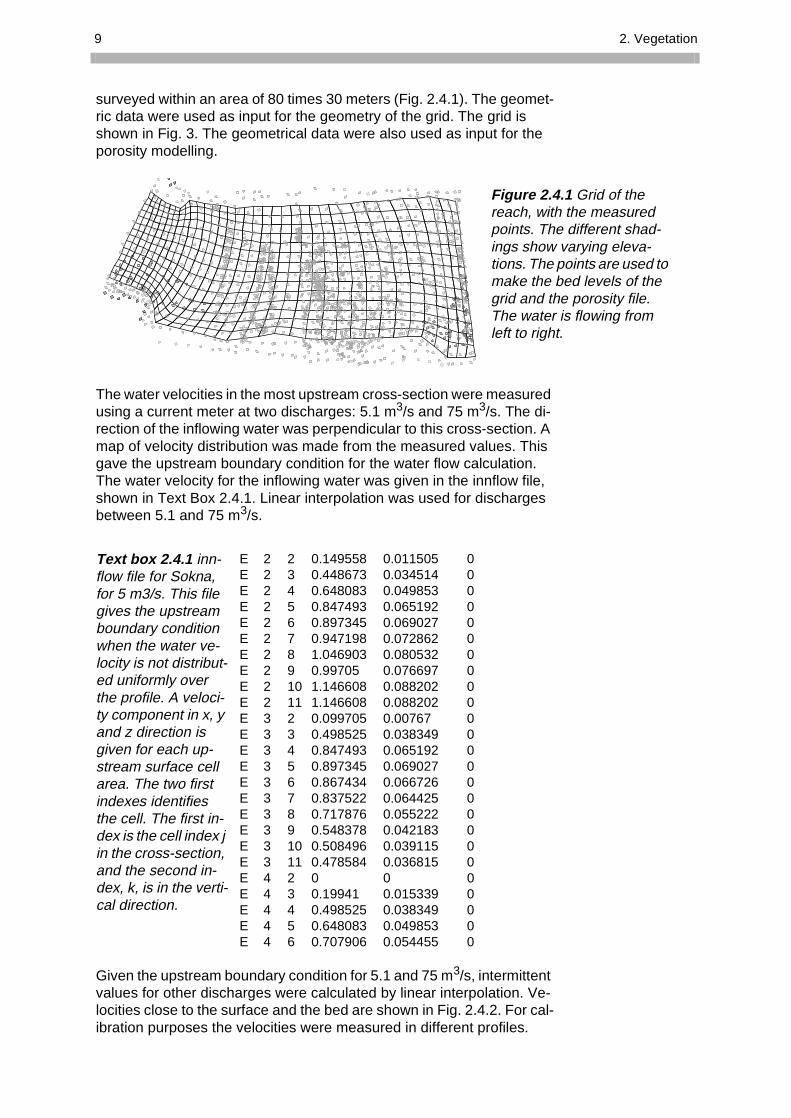
Grid of the the measured different shad-arying eleva-ints are used to d levels of the porosity file. flowing from

surveyed within an area of 80 times 30 meters (Fig. 2.4.1). The geomet-ric data were used as input for the geometry of the grid. The grid is shown in Fig. 3. The geometrical data were also used as input for the porosity modelling.

The water velocities in the most upstream cross-section were measured using a current meter at two discharges: 5.1 m3/s and 75 m3/s. The di-rection of the inflowing water was perpendicular to this cross-section. A map of velocity distribution was made from the measured values. This gave the upstream boundary condition for the water flow calculation. The water velocity for the inflowing water was given in the innflow file, shown in Text Box 2.4.1. Linear interpolation was used for discharges between 5.1 and 75 m3/s.

Given the upstream boundary condition for 5.1 and 75 m3/s, intermittent values for other discharges were calculated by linear interpolation. Ve-locities close to the surface and the bed are shown in Fig. 2.4.2. For cal-ibration purposes the velocities were measured in different profiles.

Figure 2.4.1reach, with points. The ings show vtions. The pomake the begrid and theThe water isleft to right.

E 2 2 0.149558 0.011505 0E 2 3 0.448673 0.034514 0E 2 4 0.648083 0.049853 0E 2 5 0.847493 0.065192 0E 2 6 0.897345 0.069027 0E 2 7 0.947198 0.072862 0E 2 8 1.046903 0.080532 0E 2 9 0.99705 0.076697 0E 2 10 1.146608 0.088202 0E 2 11 1.146608 0.088202 0E 3 2 0.099705 0.00767 0E 3 3 0.498525 0.038349 0E 3 4 0.847493 0.065192 0E 3 5 0.897345 0.069027 0E 3 6 0.867434 0.066726 0E 3 7 0.837522 0.064425 0E 3 8 0.717876 0.055222 0E 3 9 0.548378 0.042183 0E 3 10 0.508496 0.039115 0E 3 11 0.478584 0.036815 0E 4 2 0 0 0E 4 3 0.19941 0.015339 0E 4 4 0.498525 0.038349 0E 4 5 0.648083 0.049853 0E 4 6 0.707906 0.054455 0

Text box 2.4.1 inn-flow file for Sokna, for 5 m3/s. This file gives the upstream boundary condition when the water ve-locity is not distribut-ed uniformly over the profile. A veloci-ty component in x, y and z direction is given for each up-stream surface cell area. The two first indexes identifies the cell. The first in-dex is the cell index j in the cross-section, and the second in-dex, k, is in the verti-cal direction.


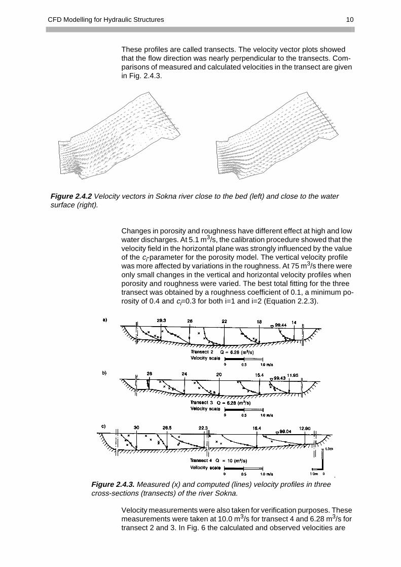
Figure 2.4.2 Velocitsurface (right).

Figure cross-se

These profiles are called transects. The velocity vector plots showed that the flow direction was nearly perpendicular to the transects. Com-parisons of measured and calculated velocities in the transect are given in Fig. 2.4.3.

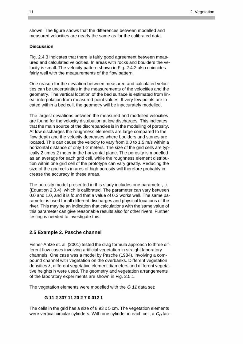
Changes in porosity and roughness have different effect at high and low water discharges. At 5.1 m3/s, the calibration procedure showed that the velocity field in the horizontal plane was strongly influenced by the value of the ci-parameter for the porosity model. The vertical velocity profile was more affected by variations in the roughness. At 75 m3/s there were only small changes in the vertical and horizontal velocity profiles when porosity and roughness were varied. The best total fitting for the three transect was obtained by a roughness coefficient of 0.1, a minimum po-rosity of 0.4 and ci=0.3 for both i=1 and i=2 (Equation 2.2.3).

Velocity measurements were also taken for verification purposes. These measurements were taken at 10.0 m3/s for transect 4 and 6.28 m3/s for transect 2 and 3. In Fig. 6 the calculated and observed velocities are

Level 11y vectors in Sokna river close to the bed (left) and close to the water

2.4.3. Measured (x) and computed (lines) velocity profiles in three ctions (transects) of the river Sokna.

11 2. Vegetation

shown. The figure shows that the differences between modelled and measured velocities are nearly the same as for the calibrated data.

Discussion

Fig. 2.4.3 indicates that there is fairly good agreement between meas-ured and calculated velocities. In areas with rocks and boulders the ve-locity is small. The velocity pattern shown in Fig. 2.4.2 also coincides fairly well with the measurements of the flow pattern.

One reason for the deviation between measured and calculated veloci-ties can be uncertainties in the measurements of the velocities and the geometry. The vertical location of the bed surface is estimated from lin-ear interpolation from measured point values. If very few points are lo-cated within a bed cell, the geometry will be inaccurately modelled.

The largest deviations between the measured and modelled velocities are found for the velocity distribution at low discharges. This indicates that the main source of the discrepancies is in the modelling of porosity. At low discharges the roughness elements are large compared to the flow depth and the velocity decreases where boulders and stones are located. This can cause the velocity to vary from 0.0 to 1.5 m/s within a horizontal distance of only 1-2 meters. The size of the grid cells are typ-ically 2 times 2 meter in the horizontal plane. The porosity is modelled as an average for each grid cell, while the roughness element distribu-tion within one grid cell of the prototype can vary greatly. Reducing the size of the grid cells in ares of high porosity will therefore probably in-crease the accuracy in these areas. The porosity model presented in this study includes one parameter, ci (Equation 2.3.4), which is calibrated. The parameter can vary between 0.0 and 1.0, and it is found that a value of 0.3 works well. The same pa-rameter is used for all different discharges and physical locations of the river. This may be an indication that calculations with the same value of this parameter can give reasonable results also for other rivers. Further testing is needed to investigate this.

2.5 Example 2. Pasche channel

Fisher-Antze et. al. (2001) tested the drag formula approach to three dif-ferent flow cases involving artificial vegetation in straight laboratory channels. One case was a model by Pasche (1984), involving a com-pound channel with vegetation on the overbanks. Different vegetation densities λ, different vegetative element diameters and different vegeta-tive heights h were used. The geometry and vegetation arrangements of the laboratory experiments are shown in Fig. 2.5.1.

The vegetation elements were modelled with the G 11 data set:

G 11 2 337 11 20 2 7 0.012 1

The cells in the grid has a size of 8.93 x 5 cm. The vegetation elements were vertical circular cylinders. With one cylinder in each cell, a CD fac-


tor of 1.0 and a cylinder diameter of 1.2 cm, the second-last parameter on the G 11 data set becomes:

Figure 2.5.2 shows the comparison of simulated results against ob-served velocity. The reduction of flow velocities through the vegetation elements can be simulated fairly well.

Fischer-Antze et al. (2001) also tested the model with varying number of grid densities, and obtained very good results for both fine and coarse grids. The water flow direction was fairly perpendicular to the grid for this case, so there were very little false diffusion.

CDnd 1.0x1x0.012 0.012= =

Figure 2.5.1 Cross-section of Pasche’s channel, showing an overbank with vege-tation rods and a main channel with-out.

a.

0.0

0.1

0.2

0.3

0.4

0.5

0 0.2 0.4 0.6 0.8 1W idth [m]

u [m

/s]

calculated measured

Figure 2.5.2 Ve-locity profile in the channel. The direction is op-posite of Fig. 2.5.1.

13 3. Spillways

3. Spillways

The hydraulic design of a spillway involves two problems:

1. Determination of coefficient of discharge2. Dissipation of the energy downstream.

Problem 2 is often more complex, as air entrainment causes two-phase flow. The algorithms described in the following is mainly focused on one-phase flow, and are therefore limited when modelling problem 2.

Early work on modelling spillways include a demonstration case from FLOW3D modelling a Parshall flume. This was presented as a demo at the IAHR Biennial Conference in London in 1995 and later by Richard-son (1997). FLOW3D uses a volume of fluid method (described below) on an orthogonal grid. Later work was given by Kjellesvig (1996) and Olsen and Kjellesvig (1998b), computing some of the examples given in the following chapters. Spaliviero and May (1998) used FLOW3D to computed coefficient of discharge for a spillway. Yang and Johansson (1998) computed coefficient of discharge for the same spillway using three CFD models (CFX, FLUENT and FLOW3D), and found the CFX model to give best results. The suggested reason was that the adaptive grid gave a more accurate location of the water surface.

3.1 Algorithms for free surface flow

There are a number of different methods to compute the location of the free surface in a CFD model:

1. 1D backwater computation2. 2D depth-averaged approach,3. Using the 3D pressure field4. Using water continuity in the cell closest to the water surface 5. The volume of fluid (VOF) method

The methods are described in more details in the following.

1D backwater computation

The 1D backwater computation is based on a friction loss, If, computed by Mannings formula:

(3.1.1)

U is the average velocity, n is Manning’s friction coefficient and r is the hydraulic radius of the flow. The 1D backwater computation uses the fol-lowing formula to compute the water elevation difference, ∆z, between two cross-sections 1 and 2:

(3.1.2)

IfnU

r

13---

-----------=

∆z If∆xU1

2

2g---------

U22

2g---------–

+=


The horizontal distance between the cross-sections is denoted ∆x, and g is the acceleration of gravity.

2D Depth-averaged approach

In a depth-averaged approach, it is assumed that the pressure distribu-tion in the vertical direction is hydrostatic. This gives a direct proportion-ality between the pressure, P, and the water depth, H:

(3.1.3)

The water density is denoted ρ. When the 2D CFD model computes the water depth, Eq. 3.1.3 is used, and after convergence, the water depth is also found.

Using the 3D pressure field

This method is often used when the water surface slope is not very large, but still has a spatial variation significant to be of interest. The principle is first to compute the pressure at the water surface.This is done by linear extrapolation from the surface cell and the cell below. The pressure is then interpolated from the cells to the grid intersections. Then a reference point is chosen, which does not move. This can typi-cally be a downstream boundary for subcritical flow. Then the pressure difference between the each grid intersection and the reference point is computed. This is assumed to be linearly proportional to the elevation difference between the two points, according to:

(3.1.4)

z is the level of the water surface, P is the pressure at the water surface, ρ is the water density and g is acceleration of gravity. The index of the variables are r for the reference point and i,j for the grid intersections.

The water surface is then moved for every n’th iteration, where n is de-termined by the user. After each movement, the grid is regenerated be-fore the computation proceeds.

Using water continuity in the cell closest to the water surface

This method is used by SSIIM in all computations of coefficient of dis-charge for spillways.

Most often, the gravity term is not included in the solution of the Navier-Stokes equations for computing river flow. This is because the gravity term is a very large source term and introduces instabilities. However, when the water surface is complex and an unknown part of the solution, the gravity term have to be included.

Normally, the SIMPLE method is used to compute the pressure in the whole domain. The pressure correction is based on the water continuity defect in each cell. The current method is based on using the SIMPLE method to compute the pressure in each cell except the cells bordering the water surface. Instead, the pressure in these cells are interpolated

P ρgH=

zij zr–Pij Pr–( )

ρg-----------------------=

15 3. Spillways

from the pressure at the surface and the pressure in the cell below the surface cell.

Volume of fluid method

This method is not used by SSIIM, but it is often used by other CFD models, computing free surfaces with complex shapes.

The main principle is to do a two-phase flow calculation, where the grid is filled with water and air. The fraction of water in each cell is computed. The location of the water surface is then computed to be in the cells with partial fraction of water. This allows for a very complex water surface, with air pocket inside the water and parts of water in the air. Such com-plexity is often encountered in hydraulic jumps downstream spillways.

Note that the grid is kept fixed trough out the computation. This gives a more stable solution, but some reduction in the accuracy may follow.


A spillway has fairly complex water surface, so it is necessary to use a fully 3D approach. Initially, it was tested if the pressure method could be used to model the spillway. This did not give any physically realistic re-sult. In all successful cases using SSIIM, the method of using water con-tinuity defect in the cell closest to the water surface has been used.

This method is invoked by specifying F 36 1 in the control file. The meth-od adds gravity to the Navier-Stokes equations in the vertical direction. Since this is a very large source term, the solution becomes unstable. A transient computation must be used, with very short time step. The time step is given on the F 33 data set. The first parameter is the time step, and the second parameter is the inner iterations for each time step. Ex-perience shows that it is advisable to use a shorter time step and keep a low number of inner iterations instead of vice versa. To improve stabil-ity, very low relaxation coefficients should also be used. A typical data set in the control file can be: K 3 0.1 0.1 0.1 0.02 0.05 0.05

Often, the spillway itself is vertical on the upstream side. This is usually modelled by blocking out cells in the spillway. The G 13 data set is then used.

The principle is to use a submerged spillway as the initial grid. Then the water surface adjusts itself to the flow field. Experience shows that using the default zero-gradient boundary condition gives better stability than using the G 7 data sets. If G 7 data sets are used, they must be used for all inflow and outflow boundaries.

3.3 Example 1. Standard spillway

The standard type spillway has a longitudinal bed profile corresponding to the theoretical shape of a free-fall spillway (US Bureau of Reclama-tion, 1973). The computed velocity field and water level at different times are given in Fig. 3.3.1. The computation starts with a horizontal water


Figure 3.3.1 Longituof discharge for a sp

surface. This is then updated based on the algorithm using a gravity term and water continuity for the cells closest to the water surface.

The spillway itself is modelled as an outblocked region, using the G 13 data set. A more detailed example on how this can be done is given in the next chapter. The computation is very unstable, so a very small time step is used, together with low relaxation coefficients. This is given on the following data sets, taken from the original control file:

F 33 0.0005 1 K 3 0.1 0.1 0.1 0.02 0.1 0.1

The specification of the boundary condition for the inflow/outflow and the water levels upstream and downstream is given in the timei file. The fol-lowing file was used for this case:

I 0.0 1.0 -1.0 -1.5 -0.5 I 120 1.0 -1.0 -1.5 -0.5

Each line in the timei file starts with a character. The I data set specifies a data set at a certain time. The time is given as the first number on the data set. In this case, there are only two data sets, at 0 and 120 sec-onds. The data sets that follow, are similar. A linear interpolation be-tween the data sets are used, for times between 0 and 120 seconds.

The data set after the time step is the inflowing water discharge: 1 m3/s. Then the outflowing water discharge is given. A negative number means that a zero gradient boundary condition is used, and the outflow water discharge is not specified. This is the only option that gives sufficient sta-bility for the computation to converge. A fixed downstream water dis-charge will not be correct anyway, as it will vary over time as the water level varies.

dinal profile of the water level and velocities for computation of coefficient illway. The numbers show the computed time.

0.5 sec.

5 ms

93 sec.

50 ms

17 3. Spillways

and trac-

The two last numbers are the upstream and downstream water level. Negative numbers are given, which means SSIIM tries to compute the values. The upstream water level has to be computed by the program, as this is used to find the coefficient of discharge. It is also very difficult to know the downstream water level, so the solution is to let the program compute it.

The deviation between the computed coefficient of discharge and the one given by US Bureau of Reclamation (1973) was 0.5 %.

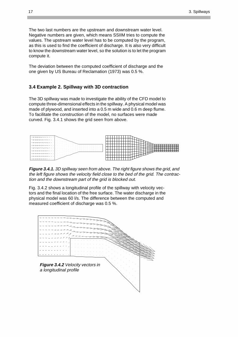
3.4 Example 2. Spillway with 3D contraction

The 3D spillway was made to investigate the ability of the CFD model to compute three-dimensional effects in the spillway. A physical model was made of plywood, and inserted into a 0.5 m wide and 0.6 m deep flume. To facilitate the construction of the model, no surfaces were made curved. Fig. 3.4.1 shows the grid seen from above.

Fig. 3.4.2 shows a longitudinal profile of the spillway with velocity vec-tors and the final location of the free surface. The water discharge in the physical model was 60 l/s. The difference between the computed and measured coefficient of discharge was 0.5 %.

Figure 3.4.1. 3D spillway seen from above. The right figure shows the grid,the left figure shows the velocity field close to the bed of the grid. The contion and the downstream part of the grid is blocked out.

Figure 3.4.2 Velocity vectors in a longitudinal profile


Defining the outblocked region

The spillway has a vertical upstream side. The only way to model such a structure in SSIIM is to block out some cells. Comparing Fig. 3.4.2 and Fig. 3.4.3, it can be seen which cells are blocked out. The outblocking is defined in the initial grid, shown in Fig. 3.4.4.

Looking at Fig. 3.4.4, the outblocked region is from i=13 to i=35 in the streamwise direction. In the vertical direction, the outblocked region is from k=2 to k=6. The transverse direction has 10 cells, numbered from 2 to 11. The data set in the control file to block out the cells becomes:

G 13 2 13 35 2 11 2 6

The first number, 2, indicates that wall laws are to be used at the top of the outblocked region. The six following numbers indicate the first and last cell number in the three directions.

For the spillway case, the water level will move. The size of the grid cells below the water level will then change in magnitude. However, it is im-portant that the top of the outblocked region does not move. Another

Blocked out

Figure 3.4.3 Longitudinal profile of the grid for the converged solution

i=2 i=13

i=35

Figure 3.4.4 Longitudinal grid at start of com-putation. The cell numbers are indicated. The block starts at i=13 in the horizontal direction. It ends at k=6 in the vertical direction.

k=2

k=6

k=11

19 3. Spillways

problem is to specify the slope of the downstream part of the spillway bed, on top of the outblocked region.

SSIIM distributes the grid cells in the vertical direction according to a ta-ble given on the G 3 data set. The table gives the vertical distance for each grid line above the bed as a percentage of the water depth. For the current case, the data set is given as:

G 3 0.0 10 20 30 40 50 60 70 80 90 100

There are 11 lines and 10 cells in the vertical direction. The first line is located at 0.0 % of the depth, the second line at 10 % of the depth etc. The top of the outblocked region is at the fifth grid line, or at 50 % of the water depth. Looking at Fig. 3.4.4, this means that the slope of the spill-way is 50 % of the slope of the grid at the lowest level. Since the lowest level is inside the block, there is no water there. The level can then be chosen so that the top of the block corresponds with the correct slope. The level at the bed or bottom of the block is given in the koordina file, which was generated by a spreadsheet.

An alternative approach would have been to use several G 16 data sets. These data sets specify a local grid distribution, similar to the G 3 data set. But before the distribution itself, four integers are read. This gives the location of the part of the grid where the data set is applied. The G 16 data sets are further described in Chapter 5.5.

3.5 Example 3. Shock waves

The shock wave is a classical test case for CFD modelling of supercrit-ical flow. Flow with high Froude number in a channel encounters a con-traction. This causes a standing wave to form, also called a shock wave.

The engineering problem of a shock wave is related to the design of spillways. Downstream a spillway the shock waves may form, and the structure needs to be designed to handle the increase in water depth.

The size and shape of the wave can be analysed using simplified theory, assuming hydrostatic pressure in the vertical direction etc. Measure-ments of shock waves in physical models have shown that 3D effects influence the results.

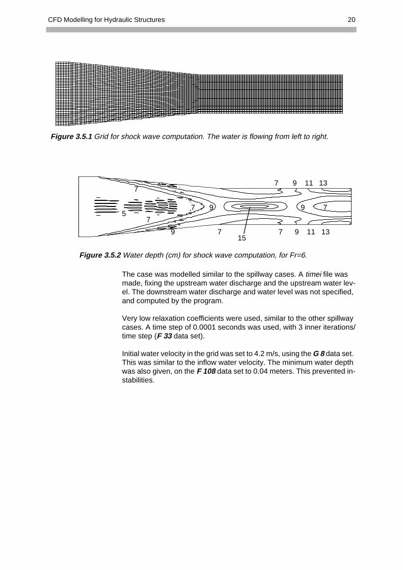
In the following, a physical model test case done by Reinauer (1984) was used. A 1 meter wide horizontal channel has an inlet with water depth 5 cm, and a Froude number of 6. The channel contracts, as shown in the grid in Fig. 3.5.1.

The case was computed by Krüger and Olsen (2001). The water velocity was relatively uniform throughout the domain, but the water depth var-ied, forming shock waves. The result (Fig. 3.5.2) is according to classi-cal theory and Reinauers experiments, but the maximum water depth is underpredicted. This may be due to air entrainment in the physical mod-el, which is not included in the CFD model.


Figure 3.5.1 Grid fo

Figure 3.5.

The case was modelled similar to the spillway cases. A timei file was made, fixing the upstream water discharge and the upstream water lev-el. The downstream water discharge and water level was not specified, and computed by the program.

Very low relaxation coefficients were used, similar to the other spillway cases. A time step of 0.0001 seconds was used, with 3 inner iterations/time step (F 33 data set).

Initial water velocity in the grid was set to 4.2 m/s, using the G 8 data set. This was similar to the inflow water velocity. The minimum water depth was also given, on the F 108 data set to 0.04 meters. This prevented in-stabilities.

r shock wave computation. The water is flowing from left to right.

5 7

7 9

77

9 9 7 7 11 13

9 11 13

9 7

15

2 Water depth (cm) for shock wave computation, for Fr=6.

21 4. Local scour

4. Local scour

Modelling local scour firstly requires the modelling of the water flow field around an obstacle. The bed shear stress is then found, and it is possi-ble to assess the potential for erosion. If movement of the bed is predict-ed, it is possible to try to predict the shape and magnitude of the scour hole. Then a computation with the new geometry can be carried out. Af-ter some iteration, it is possible to estimate the size of the scour hole. This approach was used by Richardson and Panchang (1998).

Olsen and Melaaen (1993) used a slightly different approach. The bed shear stress was used to compute the bed changes assuming a long time step with steady flow. This was iterated 10 time steps, giving a scour hole shape very similar to what was obtained in a physical model study. But neighter the CFD case nor the physical model test was run to equilibrium scour hole depth occurred. But this was later done by Olsen (1996) and Olsen and Kjellesvig (1998). This example is explained in more detail in Chapter 4.3.

Later, Roulund (2000) also computed maximum local scour hole depth using a similar approach as Olsen and Kjellesvig. Roulund, however, used a finer grid and the k-ω model instead of the k-ε model. Roulund also carried out a detailed physical modelling experiment to evaluate the CFD results.

4.1 Sediment transport modelling

Sediment transport is computed by solving the convection-diffusion equation for suspended sediment transport in addition to computing the bed load transport. Details are given by Olsen (1999).

Special algorithms for erosion on a sloping bed

The local scour case showed that the algorithms for erosion on a sloping bed is very important. There are two main algorithms:

1. Reduction in the critical shear stress 2. Sand slides

If the bed slopes upwards or sideways compared to the velocity vector, the critical shear stress for the particle will change. The decrease factor, K, as a function of the sloping bed was given by Brooks (1963):

(4.1.1)

The angle between the flow direction and a line normal to bed plane is denoted α. The slope angle is denoted φ and θ is a kind of angle of re-pose for the sediments. θ is actually an empirical parameter based on flume studies. The factor K is multiplied with the critical shear stress for

Kφ αsinsin

θtan-----------------------–

φ αsinsinθtan

----------------------- cos

2φ 1φtanθtan

----------- 2

––+=


a horizontal surface to give the effective critical shear stress for a sedi-ment particle.


The grid around the obstacle needs to be made. Often, an outblocking of the grid is used to model the geometry. The outblocking of the cells are given on the G 13 data set in the control file.

Data on the sediment type need to be given. This is done on the S data set in the control file, where sediment particle size and diameter is given. For non-uniform sediment grain size distribution, several particle sizes can be modelled simultaneously. Each size is then given on one S data set. The data sets are numbered, so that the coarsest size is given on the S 1 data set, the second coarsest size given on the S 2 data set etc. The fraction of each sediment size in the bed material is given on the N data sets. If there are n number of sediment sizes, there must also be n number of N data sets.

The algorithm for reduction of the shear stress as a function of the slop-ing bed is invoked by specifying F 7 B in the control file. The slope pa-rameter in Brook’s formula can be given on the F 109 data set. Default values are:

F 109 1.23 0.78 0.2

The two first floats are tan(θ) for uphill and downhill slopes, where θ is given in Eq. 4.1.1. The third float is a minimum value for the reduction factor. The default values were hard-coded in earlier versions of SSIIM.

The sand slide algorithm is invoked by using the F 56 data set. Two numbers are given, first an integer and then a float. The float is tan (an-gle of repose). When a grid line steeper then specified is encountered, this is corrected by the sand slide algorithm. However, after the correc-tion, the neighbouring grid lines may be steeper then specified, even if they were not before the correction. To handle the problem, al the lines are checked several times. The number of times is given on the first in-teger on the data set.

4.3 Example: Scour around a circular cylinder

The circular cylinder is the most commonly used case when studying lo-cal scour. There exist a number of empirical formulas for the scour depth. Also, studies have been made describing the scour process and evolution of the scour hole.The case presented here was done by Olsen and Kjellesvig (1998a). A cylinder with diameter 1.5 meter was used in a 8.5 meter wide and 23 meter long flume. The water depth was 2 me-ters, and the upstream average water velocity was 1.5 m/s. The sedi-ments on the bed had a uniform distribution with average diameter 20 mm.

The grid had 70x56x20 cells in the streamwise, lateral and vertical direc-tion, respectively. The grid seen from above is given in Fig. 4.3.1. The

23 4. Local scour

-

time step for the computation was 100 seconds, and a total of 1.5 million seconds were computed. The scour depth in front of the cylinder as a function of the computed time decreased similarly as given in Fig. 4.3.2. The steady state scour hole then had a geometry shown in Fig. 4.3.3. The maximum scour depth compared reasonably well with empirical for-mulas (Olsen and Kjellesvig, 1998a).

The sediments were modelled on the S data set, with the following val-ues: S 1 0.02 1.75. The last number is the fall velocity of the sediments. A value of 1.75 m/s was used. The current case was clear-water scour, so now sediment inflow was given the I data set therefore was: I 1 0.0

Figure 4.3.1 Grid of the cylinder, seen from above. The water flow direction is from left to right.

Figure 4.3.2 Exam-ple of time series of bed elevation in front of the cylinder (p.s. not from this case)


(i=18,j=19

(i=11,j=12

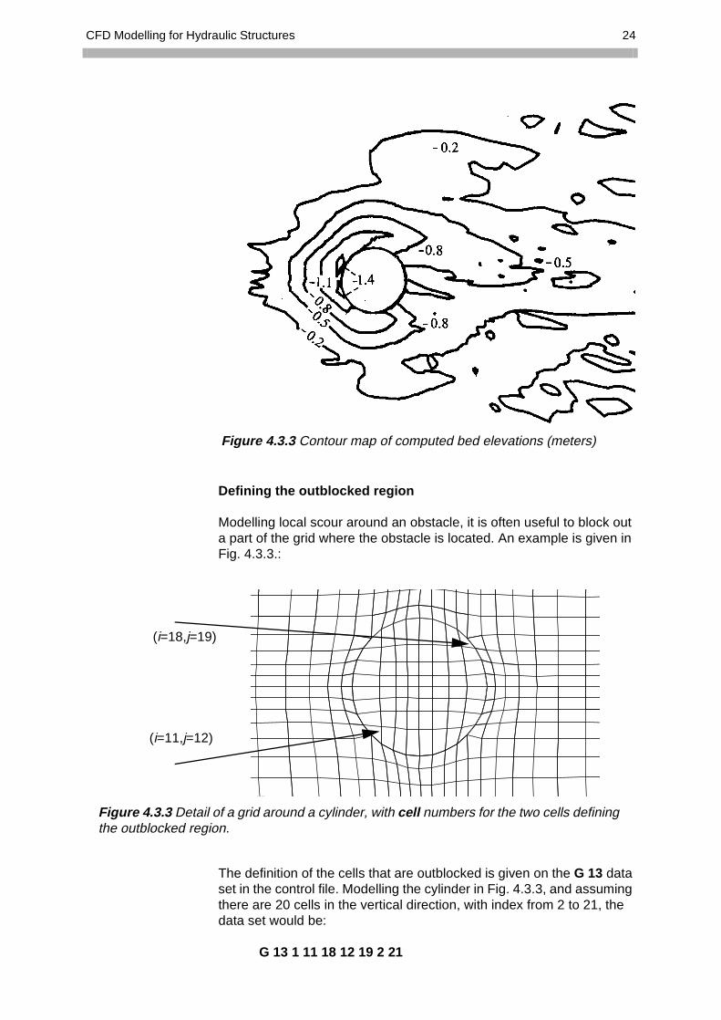
Figure 4.3.3 Detailthe outblocked reg

Defining the outblocked region

Modelling local scour around an obstacle, it is often useful to block out a part of the grid where the obstacle is located. An example is given in Fig. 4.3.3.:

The definition of the cells that are outblocked is given on the G 13 data set in the control file. Modelling the cylinder in Fig. 4.3.3, and assuming there are 20 cells in the vertical direction, with index from 2 to 21, the data set would be:

G 13 1 11 18 12 19 2 21

Figure 4.3.3 Contour map of computed bed elevations (meters)

Level 2

)

)

of a grid around a cylinder, with cell numbers for the two cells defining ion.

25 4. Local scour

ound-ers in

The first integer indicates which sides of the outblocked region has wall laws. The index 1 defines wall laws on the vertical sides. It is also pos-sible to model a submerged outblocked region, in which case the index should be 2. Such cases are described in Chapter 3.

When making the G 13 data set, it is advisable to test the numbers by looking at the grid in SSIIM. Red lines will be shown around the out-blocked region when velocity vectors are shown. Then it usually can be seen if the correct numbers are given.

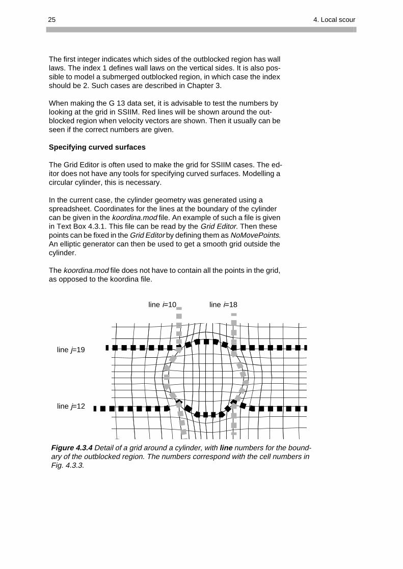
Specifying curved surfaces

The Grid Editor is often used to make the grid for SSIIM cases. The ed-itor does not have any tools for specifying curved surfaces. Modelling a circular cylinder, this is necessary.

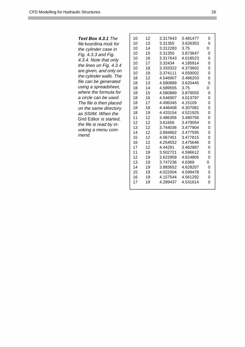
In the current case, the cylinder geometry was generated using a spreadsheet. Coordinates for the lines at the boundary of the cylinder can be given in the koordina.mod file. An example of such a file is given in Text Box 4.3.1. This file can be read by the Grid Editor. Then these points can be fixed in the Grid Editor by defining them as NoMovePoints. An elliptic generator can then be used to get a smooth grid outside the cylinder.

The koordina.mod file does not have to contain all the points in the grid, as opposed to the koordina file.

Level 2

line j=19

line j=12

line i=10 line i=18

Figure 4.3.4 Detail of a grid around a cylinder, with line numbers for the bary of the outblocked region. The numbers correspond with the cell numbFig. 4.3.3.


10 12 3.317643 3.481477 0 10 13 3.31355 3.626353 0 10 14 3.312283 3.75 0 10 15 3.31355 3.873647 0 10 16 3.317643 4.018523 0 10 17 3.32434 4.185914 0 10 18 3.333322 4.373602 0 10 19 3.374111 4.559002 0 18 12 4.546907 3.486203 0 18 13 4.580889 3.620445 0 18 14 4.589555 3.75 0 18 15 4.580889 3.879555 0 18 16 4.546907 4.013797 0 18 17 4.496345 4.15109 0 18 18 4.446408 4.307081 0 18 19 4.433154 4.521925 0 11 12 3.486356 3.480756 0 12 12 3.61656 3.479054 0 13 12 3.744036 3.477904 0 14 12 3.894862 3.477595 0 15 12 4.067451 3.477815 0 16 12 4.254552 3.475646 0 17 12 4.44291 3.462987 0 11 19 3.502721 4.596612 0 12 19 3.622959 4.624805 0 13 19 3.747236 4.6369 0 14 19 3.883652 4.628207 0 15 19 4.022004 4.599478 0 16 19 4.157544 4.561292 0 17 19 4.289437 4.531614 0

Text Box 4.3.1 The file koordina.mod for the cylinder case in Fig. 4.3.3 and Fig. 4.3.4. Note that only the lines on Fig. 4.3.4 are given, and only on the cylinder walls. The file can be generated using a spreadsheet, where the formula for a circle can be used. The file is then placed on the same directory as SSIIM. When the Grid Editor is started, the file is read by in-voking a menu com-mend.

27 5. Intakes

SSIIM is an acro-nym for Sediment Simulation In In-takes with Multi-block option

5. Intakes

Design of run-of-river water intakes is a particular problem in sediment-carrying rivers. Often, a physical model study is done to assist in hydrau-lic design. However, it is very difficult to model fine sediments in a phys-ical model. This was the main motivation for making the SSIIM model. The SSIIM model has been used to compute trap efficiency of a sand trap (Olsen and Skoglund, 1994), also shown in Chapter 5.3. Later it has been used to model bed changes in a sand trap (Olsen and Kjellesvig, 1998), further described in Chapter 5.4. Flow in a very complex intake structure, the Himalayan Intake is presented in Chapter 5.5.

Complex intakes has also been modelled by Demny et. al. (1998), using an in-house finite element model of the Aachen University of Technolo-gy, Germany. Sediment flow in intakes has been computed by Atkinson (1995), for two prototype cases. The CFD model PHOENICS was used.

5.1 Intake design and sediment problems

Most hydraulic structures will be surrounded by a fairly complex three-dimensional flow field. For water flow with sediments, the suspended particles will move with the flow. A good hydraulic design of an run-of-the-river intake is often essential for its performance.

There are some hydraulic principles involved in the intake design. One guideline is to avoid recirculation zones. These create turbulence, keep-ing suspended sediments in the water for a longer time, instead of set-tling out. When it comes to bed load, the creation of secondary currents is often used to prevent the sediments from entering the intake. An ex-ample is to have the intake located at the outside of a river bend, using the natural secondary current to sweep the bed load away from the in-take. It is also possible to use the secondary currents emerging from flow around obstructions to move the bed load away from the intake.

A CFD model including all these processes has to be fully three-dimen-sional, capable of modelling both secondary currents, recirculation zones and turbulence. It also should take into account bed changes as a function of sediment deposition/scour.

5.2 Modelling complex structures with SSIIM

Often, a hydraulic structure is best modelled by SSIIM 1. This is because of its outblocking options and the possibility to create walls along grid lines. A hydraulic structure often has vertical walls with channel open-ings, and this is problematic to model for SSIIM 2. The outblocked areas are modelled with the G 13 data sets in the control file. The walls be-tween cells are modelled with the W 4 data set.

An intake may also have a complex inflow and outflow. The default in-flow for SSIIM 1 is over the whole of the upstream cross-section. And the default outflow is over the whole downstream cross-section. The sides are modelled with walls as default. It is possible to change this, by


adding walls to parts of the upstream or downstream cross-section. Or specifying inflow/outflow on the side walls or in the bed. Removing or adding walls are done with the W 4 data set. Specifying inflow/outflow is done with the G 7 data set. Note that if the G 7 data set is used, one should specify inflow/outflow over the whole geometry, and not use the default inflow/outflow. Also, the W 4 data set must be used to remove the walls in the areas where the G 7 data set is used.

The water surface is modelled with zero gradients as default, but it is also possible to change this. There are two approaches:

1. Specify a closed conduit simulation on the K 2 data set2. Add walls on the surface by using the W 4 data set

If option 1 is used, the option K 2 0 0 should be used. The coordinates for the top of the geometry then has to be given in the koordina file. An extra double is then given on each line, specifying the vertical elevation of the roof of the conduit. This can also be used to model a curved roof.

If option 2 is used, the wall is specified with the W 4 data set and 3 -1 as the first and second integer.

Note that multiple G 7, G 13 and W 4 data sets can be given, enabling multiple walls, outblocked cells and inflow/outflows.

The default sediment inflow is at the upstream cross-section, and it is specified with the I data set of the control file. There is one I data set for each sediment fraction. This will distribute the sediment over the up-stream cross-section, so if this is partially blocked out by walls or out-blocked cells, the specification will not be correct. Then the G 20 data set should be used instead. This can also be used if there is sediment inflow from other locations than the upstream cross-section.

Modelling an intake, it is sometimes important to know how much sedi-ments enter the intake, and how much enters the spillway area. This can be determined using multiple G 21 data set. A region is then defined, where the water and sediment flows through. For each G 21 data set, the sediment flux will be written to the boogie file.

5.3 Example 1. Sediment deposition in a sand trap

The flow of water and sediments in a three-dimensional sand trap was calculated for a steady-state situation. A physical model study carried out to verify the results. It showed the recirculation zone to be shorter than the numerical model result, but modifications in the k-ε turbulence model gave better agreement. The sediment concentration calculations compare well with the experimental procedures. The concentration cal-culated by using the flow field from the original k-ε model gave 87.1 % trap efficiency, whereas calculation with the more correct flow field gave 88.3 %.

29 5. Intakes

eft to right. The

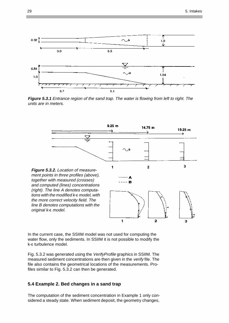
In the current case, the SSIIM model was not used for computing the water flow, only the sediments. In SSIIM it is not possible to modify the k-ε turbulence model.

Fig. 5.3.2 was generated using the VerifyProfile graphics in SSIIM. The measured sediment concentrations are then given in the verify file. The file also contains the geometrical locations of the measurements. Pro-files similar to Fig. 5.3.2 can then be generated.

5.4 Example 2. Bed changes in a sand trap

The computation of the sediment concentration in Example 1 only con-sidered a steady state. When sediment deposit, the geometry changes,

Figure 5.3.1 Entrance region of the sand trap. The water is flowing from lunits are in meters.

Figure 5.3.2. Location of measure-ment points in three profiles (above), together with measured (crosses) and computed (lines) concentrations (right). The line A denotes computa-tions with the modified k-ε model, with the more correct velocity field. The line B denotes computations with the original k-ε model.


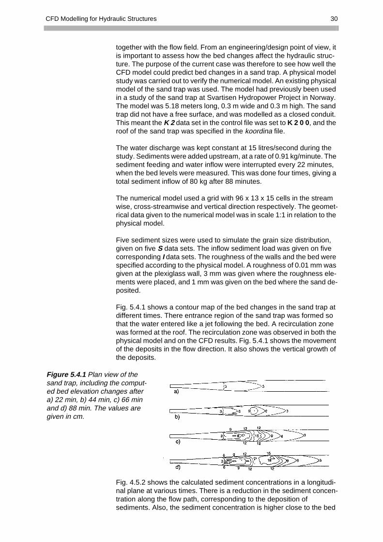
Figure 5.4.1 Plan viesand trap, including ted bed elevation chaa) 22 min, b) 44 min,and d) 88 min. The vgiven in cm.

together with the flow field. From an engineering/design point of view, it is important to assess how the bed changes affect the hydraulic struc-ture. The purpose of the current case was therefore to see how well the CFD model could predict bed changes in a sand trap. A physical model study was carried out to verify the numerical model. An existing physical model of the sand trap was used. The model had previously been used in a study of the sand trap at Svartisen Hydropower Project in Norway. The model was 5.18 meters long, 0.3 m wide and 0.3 m high. The sand trap did not have a free surface, and was modelled as a closed conduit. This meant the K 2 data set in the control file was set to K 2 0 0, and the roof of the sand trap was specified in the koordina file.

The water discharge was kept constant at 15 litres/second during the study. Sediments were added upstream, at a rate of 0.91 kg/minute. The sediment feeding and water inflow were interrupted every 22 minutes, when the bed levels were measured. This was done four times, giving a total sediment inflow of 80 kg after 88 minutes.

The numerical model used a grid with 96 x 13 x 15 cells in the stream wise, cross-streamwise and vertical direction respectively. The geomet-rical data given to the numerical model was in scale 1:1 in relation to the physical model.

Five sediment sizes were used to simulate the grain size distribution, given on five S data sets. The inflow sediment load was given on five corresponding I data sets. The roughness of the walls and the bed were specified according to the physical model. A roughness of 0.01 mm was given at the plexiglass wall, 3 mm was given where the roughness ele-ments were placed, and 1 mm was given on the bed where the sand de-posited.

Fig. 5.4.1 shows a contour map of the bed changes in the sand trap at different times. There entrance region of the sand trap was formed so that the water entered like a jet following the bed. A recirculation zone was formed at the roof. The recirculation zone was observed in both the physical model and on the CFD results. Fig. 5.4.1 shows the movement of the deposits in the flow direction. It also shows the vertical growth of the deposits.

Fig. 4.5.2 shows the calculated sediment concentrations in a longitudi-nal plane at various times. There is a reduction in the sediment concen-tration along the flow path, corresponding to the deposition of sediments. Also, the sediment concentration is higher close to the bed

w of the he comput-nges after c) 66 min alues are

31 5. Intakes

uted (A) and meas-es in the sand n the axis are in

than near the roof. This is in accordance with the theory. The figure shows the time evolution of the deposit. At the upstream end the mag-nitude of the deposit decrease as sediments are eroded at this location. This was also observed in the physical model.

Fig. 5.4.3 shows a comparison between the measured and calculated bed elevation changes after 88 minutes. There is good correspondence between the calculated and measured values. Some deviation at the start and at the front of the deposition will be discussed later.

A parameter sensitivity test was carried out to assess the effects of some important input parameters on the result. The chosen roughness (F 16 data set) affected the shear stress at the bed, which affected the sediment transport capacity. The parameter test showed that it is fairly important to use a correct roughness in the simulation.

The angle of repose for the sediments was changed from 40 degrees to 35 degrees (F 56 data set), only resulted in marginal changes. The for-mula for sediment concentration close to the bed was changed (F 6 data set), reducing the concentration by 33 %. The sediment deposits then became greater in magnitude and did not reach as far out in the sand trap as for the original simulation. This result is a logical consequence of the decrease in transport capacity. However, the changes are not very great, considering that the transport capacity was decreased by 33 %.

Figure 5.4.2 Longitudinal pro-files of the sand trap with pro-files of suspended sediment concentrations. The bed changes at the centerline of the profile is also shown, after a) 22 min, b) 44 min, c) 66 min and d) 88 min.

Figure 5.4.3 Compured (B) bed changtrap.The numbers ometers.


The numerical model was therefore not very sensitive to the accuracy of the formula for concentration at the bed for this case. Other parameter tests show very little effect of changing the number of inner iterations from 5 to 10 (F 33 data set) for each time step for the Na-vier-Stokes equations, and changing the time step 10 to 5 seconds (F 33 data set).

The deviation between the calculated and measured bed level changes can be caused by several phenomena. Fig. 5.4.3 shows that the meas-ured bed levels are lower than the calculated levels at the downstream part of the deposit. This may be caused by false diffusion as there is a recirculation zone in this region. Another explanation may be the shape of the deposit in this area. Looking at Fig. 5.4.1, after 88 minutes, the deposit is much greater at the centerline of the sand trap than at the sides. This effect is also observed in the physical model, but not to the same extent as in the calculated results.

5.5 Example 3. Complex geometries - Himalaya intake

An intake construction sometimes has a very complex geometry. One of the most complex flow cases modelled with SSIIM was the Himalayan Intake. The intake was designed by Prof. H. Støle as a mean of decreas-ing sediment problems for run-of-the-river hydropower plants taking water from steep rivers. The geometry of the CFD model was made by H. Kjellesvig (1995). (Kjellesvig and Støle, 1996).

The intake has gates both close to the surface and close to the bed. This allows both floating debris and bedload to pass the intake dam. The dam itself has a large intake in form of a tube, parallel to the dam axis. The longitudinal profiles shown in Fig. 5.5.1 are cross-sections of the dam and the tube. At the exit of this tube, the water goes to the hydropower plant. Most of the water enters at the upper part of the tube, where the sediment concentration is lowest. There is also a opening at the bottom of the tube, allowing deposited sediments to fall down into the river and be flushed out.

The tube and other parts of the intake are modelled partly as outblocked regions and partly with walls between cells. The outblocked regions are modelled with G 13 data sets, and the walls are modelled with W 4 data sets. These data sets and the corresponding location is given in Text Box 5.5.1 and Fig. 5.5.1.

Each wall that has water on both sides must be modelled with two W4 data sets. One data set will only provide wall functions for one side of the wall. In Text Box 5.5.1, the two corresponding W 4 data sets are placed after each other. As an example the data sets for wall g is given below:

W 4 1 -1 7 2 16 8 11 wall g W 4 1 1 8 2 16 8 11 wall g

33 5. Intakes

b

c

d

f

ie

Cells i=21

1 0 0 inlet a

0 0 outlet b

1 0 0 outlet c

ocked region d

h a

g

Cells i=2 Cells i=6

Figure 5.5.1 Longitudinal profile of the Himalayan In-take, close to the side facing away from the power plant (j=2). The top figure shows the walls, inlet and outlet ar-eas, where letters are also given to be described in more detail in the text. The middle figure shows the grid, with indexes for some of the cells. The lower figure shows a velocity vector plot.

G 7 0 1 2 16 2 14 0 0 126.75 G 7 1 -1 2 4 2 3 0 0 25.85 1

G 7 1 -1 2 16 12 14 0 0 37.20 G 13 3 20 21 2 16 8 11 outbl

W 4 1 -1 21 2 16 4 7 wall e

W 4 1 -1 7 2 16 8 11 wall gW 4 1 1 8 2 16 8 11 wall g

W 4 3 -1 7 8 16 2 16 wall hW 4 3 1 8 8 16 2 16 wall h

W 4 3 1 12 13 19 2 16 wall fW 4 3 -1 11 13 19 2 16 wall f

W 4 3 1 8 18 19 2 16 wall iW 4 3 -1 7 18 19 2 16 wall i

Text box 5.5.1 Data sets in the control file, defining in-flow, outflow, outblocked re-gion, internal and external walls. The letters corre-spond to Fig. 5.5.1. Note only the data sets relevant for Fig. 5.5.1 are shown.


G16 1 2 1 16 0.0 7.6G16 3 3 1 16 0.0 10.0G16 4 7 1 16 0.0 12.32G16 8 8 1 16 0.0 9.42G16 9 9 1 16 0.0 8.3G16 10 10 1 16 0.0 7G16 11 11 1 16 0.0 6G16 12 12 1 16 0.0 6G16 13 13 1 16 0.0 5G16 14 14 1 16 0.0 5G16 15 18 1 16 0.0 5G16 19 19 1 16 0.0 5G16 20 20 1 16 0.0 4G16 21 21 1 16 0.0 4

Text box 5.5.2 G 16

The first integer (1) says that the wall is in a cross-section. On the first line, the wall is in cell i=7 (third integer). The second integer, -1, says that the wall is in the direction of an increasing cell number. That is, in the direction of cell i=8.

On the second line, the wall function is in cell i=8, but the wall is now in the direction of decreasing i numbers (cell i=7).

The last four integers indicate the location of the wall in the cross-sec-tion. The fourth and fifth integer indicates the cell numbers in the trans-verse direction, from j=2 to j=16. Note that the cross-section shown in Fig. 5.5.1 is in layer j=2. The last two integers says the wall is in the ver-tical layer from k=8 to k=11. This can be verified by counting the cells in Fig. 5.5.1, noting the bed cell has cell number k=2.

Vertical distribution of grid cells

Looking at the grid in Fig. 5.5.1, the vertical distribution of grid cells var-ies greatly. The variation is given on the G 16 data sets. The distribution is made so that the location of the intake geometry should be as close to the prototype as possible. Also, the grid qualities, expansion ratio, or-thogonality etc. can be controlled by the G 16 data sets.

Text Box 5.5.2 gives all the G 16 data sets for the grid in Fig. 5.5.1.

9 15.38 23.08 30.77 38.46 46.15 53.85 61.54 69.23 76.92 84.62 92.31 100.01 20.01 30.02 40.02 50.03 60.03 64.97 69.90 74.83 79.77 86.51 93.26 100.0 24.64 36.96 49.28 61.59 73.91 76.09 78.26 80.43 82.61 88.41 94.20 100.0 18.84 28.26 37.68 47.10 58.66 65.15 71.64 78.12 84.61 89.74 94.87 100.0 3 16.67 25.00 33.33 41.67 50.00 58.06 67.13 76.50 86.26 90.85 95.44 100.0.25 14.49 21.74 28.99 36.23 43.48 50.52 63.56 76.00 87.65 91.76 95.86 100.0.38 12.75 19.13 25.51 31.88 38.26 43.48 60.87 75.00 89.13 92.75 96.38 100.0.09 12.17 18.26 24.35 30.43 37.33 43.48 60.87 75.17 89.48 92.98 96.48 100.0.65 11.30 16.96 22.61 28.26 33.91 43.48 60.87 76.09 91.30 94.20 97.10 100.0.51 11.01 16.52 22.03 27.54 33.04 43.48 60.87 76.09 91.30 94.20 97.10 100.0.36 10.72 16.09 21.45 26.81 32.17 43.48 60.87 76.09 91.30 94.20 97.10 100.0.01 10.01 15.02 20.03 25.04 30.04 41.70 59.64 75.34 91.03 94.02 97.01 100.0.55 9.09 13.64 18.18 22.73 28.18 40.91 59.09 75.00 90.91 93.94 96.97 100.0.55 9.09 13.64 18.18 22.73 27.27 40.91 59.09 75.00 90.91 93.94 96.97 100.0

data sets in the control file, defining the grid.

35 Literature

Literature

Ackers, P. and White, R. W. (1973) "Sediment Transport: New Approach and Analysis", ASCE Journal of Hydraulic Engineering, Vol. 99, No. HY11.

Atkinson, E. (1995) “A Numerical Model for Predicting Sediment Exclu-sion at Intakes”, HR Wallingford, UK, Report OD130.

Blench, T. (1970) “Regime theory design of canals with sand beds”, ASCE Journal of Irrigation and Drainage Engineering, Vol. 96, No. IR2, Proc. Paper 7381, June, pp. 205-213.

Brooks, H. N. (1963), discussion of "Boundary Shear Stresses in Curved Trapezoidal Channels", by A. T. Ippen and P. A. Drinker, ASCE Journal of Hydraulic Engineering, Vol. 89, No. HY3.

Demny, G., Rettemeier, K., Forkel, C. and Köngeter, J. (1998) “3D-numerical investigation for the intake of a river run power plant”, Hydroinformatics - 98, Copenhagen, Denmark.

Einstein, H. A., Anderson, A. G. and Johnson, J. W. (1940) “A distinc-tion between bed-load and suspended load in natural streams”, Trans-actions of the American Geophysical Union’s annual meeting, pp. 628-633.

Einstein, H. A. and Ning Chien (1955) "Effects of heavy sediment con-centration near the bed on velocity and sediment distribution", UCLA - Berkeley, Institute of Engineering Research.

Engelund, F. (1953) "On the Laminar and Turbulent Flows of Ground Water through Homogeneous Sand", Transactions of the Danish Acad-emy of Technical Sciences, No. 3.

Engelund, F. and Hansen, E. (1967) "A monograph on sediment trans-port in alluvial streams", Teknisk Forlag, Copenhagen, Denmark.

Fisher-Antze, T., Stoesser, T., Bates, P. and Olsen, N. R. B. (2001) “3D Numerical Modelling of Open-Channel Flow with Submerged Vegeta-tion”, IAHR Journal of Hydraulic Research, Vol. 39, No. 3.

Kjellesvig, H. M. and Stoele, H. (1996) "Physical and numerical model-ling of the Himalayan Intake", 2nd. International Conference on Model-ling, Testing and Monitoring for Hydro Powerplants", Lausanne, Switzerland.

Kjellesvig, H. M. (1996) “Numerical modelling of flow over a spillway”, Hydroinformatics 96, Zürich, Switzerland.

Krüger, S., Bürgisser, M., Rutschmann, P. (1998). Advances in calcu-lating supercritical flows in spillway contractions. Hydroinformatics' 98, 163-170.

Krüger, S. and Olsen, N. R. B. (2001) "Shock-wave computations in channel contractions", XXIX IAHR Congress, Beijing, China.

Lysne, D. K. (1969) “Movement of sand in tunnels”, ASCE Journal of Hydraulic Engineering, Vol. 95, No. 6, November.

Mayer-Peter, E. and Mueller, R. (1948) "Formulas for bed load trans-port", Report on Second Meeting of International Association for Hydraulic Research, Stockholm, Sweden.

Melaaen, M. C. (1992) "Calculation of fluid flows with staggered and


nonstaggered curvilinear nonorthogonal grids - the theory", Numerical Heat Transfer, Part B, vol. 21, pp 1- 19.

Olsen, N. R. B. and Melaaen, M. C. (1993) "Three-dimensional numeri-cal modelling of scour around cylinders", ASCE Journal of Hydraulic Engineering, Vol. 119, No. 9, September.

Olsen, N. R. B., Jimenez, O., Lovoll, A. and Abrahamsen, L. (1994) "Calculation of water and sediment flow in hydropower reservoirs", 1st. International Conference on Modelling, Testing and Monitoring of Hydropower Plants, Hungary.

Olsen, N. R. B. and Skoglund, M. (1994) "Three-dimensional numerical modelling of water and sediment flow in a sand trap", IAHR Journal of Hydraulic Research, No. 6.

Olsen, N. R. B. and Stokseth, S. (1995) "Three-dimensional numerical modelling of water flow in a river with large bed roughness", IAHR Jour-nal of Hydraulic Research, Vol. 33, No. 4.

Olsen, N. R. B. (1996) “Three-dimensional numerical modelling of local scour”, Hydroinformatics 96, Zürich, Switzerland.

Olsen, N. R. B. (1999) "Computational Fluid Dynamics in Hydraulic and Sedimentation Engineering", Class notes, Department of Hydraulic and Environmental Engineering, The Norwegian University of Science and Technology.

Olsen, N. R. B. and Kjellesvig, H. M. (1998a) "Three-dimensional numerical flow modelling for estimation of maximum local scour depth", IAHR Journal of Hydraulic Research, No. 4.

Olsen, N. R. B. and Kjellesvig, H. M. (1998b) "Three-dimensional numerical flow modelling for estimation of spillway capacity", IAHR Journal of Hydraulic Research, No. 5.

Olsen, N. R. B. (1999) "Two-dimensional numerical modelling of flush-ing processes in water reservoirs", IAHR Journal of Hydraulic Research, Vol. 1.

Olsen, N. R. B. and Kjellesvig, H. M. (1999) "Three-dimensional numer-ical modelling of bed changes in a sand trap", IAHR Journal of Hydraulic Research, Vol. 37, No. 2. abstract

Pasche, E. (1984) “Turbulence Mechanism in Natural Streams and the Possibility of its Mathematical Representation” (in German) Mitteilungen Institut für Wasserbau und Wasserwirtschaft No. 52. RWTH Aachen, Germany.

Patankar, S. V. (1980) "Numerical Heat Transfer and Fluid Flow", Mc-Graw-Hill Book Company, New York.

Reinauer, R. (1995). Kanalkontraktionen bei schiessendem Abfluss und Stosswellenreduktion mit Diffraktoren. PhD thesis, ETH Zurich, Diss No. 11320.

Rhie, C.-M, and Chow, W. L. (1983) "Numerical study of the turbulent flow past an airfoil with trailing edge separation", AIAA Journal, Vol. 21, No. 11.

Richardson, J. E. (1997) "Control of Hydraulic Jump by Abrupt Drop," XXVII IAHR Congress, San Francisco, USA.

37 Literature

Richardson, J. E. and Panchang, V. G. (1998) “Three-dimensional sim-ulation of scour-inducing flow at bridge piers“, ASCE Journal of Hydrau-lic Engineering, Vol. 124, No. 5, May, page 530-540.

van Rijn, L. C. (1982) “Equivalent roughness of alluvial bed”, ASCE Journal of Hydraulic Engineering, Vol. 108, No. 10.

van Rijn, L. C. (1987) "Mathematical modelling of morphological proc-esses in the case of suspended sediment transport", Ph.D Thesis, Delft University of Technology.

Roulund, A. (2000) “Three-dimensional numerical modelling of flow around a bottom mounted pile and its application to scour”, PhD Thesis, Department of Hydrodynamics and Water Resources, Technical Univer-sity of Denmark.

Schlichting, H. (1979) "Boundary layer theory", McGraw-Hill.

Shields, A. (1936) “Use of dimensional analysis and turbulence research for sediment transport”, Preussen Research Laboratory for Water and Marine Constructions, publication no. 26, Berlin (in Ger-man).

Seed, D. (1997) "River training and channel protection - Validation of a 3D numerical model", Report SR 480, HR Wallingford, UK.

Spaliviero, F. and May, R. (1998) “Numerical modelling of 3D flow in hy-draulic structures”, IAHR/SHSG seminar on Hydraulic Engineering, Glasgow, UK.

Sæterbø, E., Syvertsen, L. and Tesaker, E. (1998) “Handbook of rivers” (Vassdragshåndboka), Tapir forlag, Norway, ISBN 82-519-1290-3 (in Norwegian).

US Bureau of Reclamation (1973) “Design of small dams”, Washington, USA.

Vanoni, V., et al (1975) "Sedimentation Engineering", ASCE Manuals and reports on engineering practice - No54.

Yang, T. C. (1973) "Incipient Motion and Sediment Transport", ASCE Journal of Hydraulic Engineering, Vol. 99, No HY10.

Yang, J. and Johansson, N. (1998) “Determination of Spillway Dis-charge Capacity - CFD Modelling and Experiment Verification”, 3rd Int. Conf. on Advances in Hydroscience and -Engineering, Cottbus, Ger-many.

Wright, N. (2001) “Conveyance implications for 2-D and 3-D model-ling”, EPSRC Network on Conveyance in River/Floodplain Systems, UK, http://ncrfs.civil.gla.ac.uk/workplan.htm.

CFD for Hydraulic Structures (535 kB) - NTNUfolk.ntnu.no/nilsol/cfd/cfdstr.pdf · CFD modelling for...

Documents

Transcript of CFD for Hydraulic Structures (535 kB) - NTNUfolk.ntnu.no/nilsol/cfd/cfdstr.pdf · CFD modelling for...