Application of CFD to Safety and Thermal-Hydraulic ...435252/FULLTEXT01.pdfApplication of CFD to...
69
Master Thesis Application of CFD to Safety and Thermal-Hydraulic Analysis of Lead-Cooled Systems Marti Jeltsov Supervisor: Pavel Kudinov Division of Nuclear Power Safety Royal Institute of Technology Stockholm, Sweden June 2011 TRITA-FYS 2011:37 ISSN 0280-316X ISRN KTH/FYS/–11:37–SE
Transcript of Application of CFD to Safety and Thermal-Hydraulic ...435252/FULLTEXT01.pdfApplication of CFD to...

Master Thesis
Application of CFD to Safety and Thermal-Hydraulic Analysis ofLead-Cooled Systems
Marti Jeltsov
Supervisor:Pavel Kudinov
Division of Nuclear Power SafetyRoyal Institute of Technology
Stockholm, SwedenJune 2011
TRITA-FYS 2011:37 ISSN 0280-316X ISRN KTH/FYS/–11:37–SE

ii

ABSTRACT
Computational Fluid Dynamics (CFD) is increasingly being used in nuclear reactor safety analysis as a toolthat enables safety related physical phenomena occurring in the reactor coolant system to be described inmore detail and accuracy. Validation is a necessary step in improving predictive capability of a computationalcode or coupled computational codes. Validation refers to the assessment of model accuracy incorporatingany uncertainties (aleatory and epistemic) that may be of importance. The uncertainties must be identified,quantified and if possible, reduced.
In the first part of this thesis, a discussion on the development of an approach and experimental facilityfor the validation of coupled Computational Fluid Dynamics codes and System Thermal Hydraulics (STH)codes is given. The validation of a coupled code requires experiments which feature significant two-wayfeedbacks between the component (CFD sub-domain) and the system (STH sub-domain). Results of CFDanalysis that are used in the development of a flexible design of the TALL-3D experimental facility arepresented. The facility consists of a lead-bismuth eutectic (LBE) thermal-hydraulic loop operating in forcedand natural circulation regimes with a heated pool-type 3D test section. Transient analysis of the mixing andstratification phenomena in the 3D test section under forced and natural circulation conditions in the loopshow that the test section outlet temperature deviates from that predicted by analytical solution (which the1D STH solution essentially is). Also an experimental validation test matrix according to the key physicalphenomena of interest in the new experimental facility is developed.
In the second part of the thesis we consider the risk related to steam generator tube leakage or rupture(SGTL/R) in a pool-type design of lead-cooled reactor (LFR). We demonstrate that there is a possibilitythat small steam bubbles leaking from the SGT will be dragged by the turbulent coolant flow into the coreregion. Voiding of the core might cause threats of reactivity insertion accident or local damage (burnout)of fuel rod cladding. Trajectories of the bubbles are determined by the bubble size and turbulent flow fieldof lead coolant. The main objective of such study is to quantify likelihood of steam bubble transport tothe core region in case of SGT leakage in the primary coolant system of the ELSY (European Lead-cooledSYstem) design. Coolant flow field and bubble motion are simulated by CFD code Star-CCM+. First, wediscuss drag correlations for a steam bubble moving in liquid lead. Thereafter the steady state liquid leadflow field in the primary system is modeled according to the ELSY design parameters of nominal full poweroperation. Finally, the consequences of SGT leakage are modeled by injecting bubbles in the steam generatorregion. An assessment of the probability that bubbles can reach the core region and also accumulate inthe primary system, is performed. The most dangerous leakage positions in the SG and bubble sizes areidentified. Possible design solutions for prevention of core voiding in case of SGTL/R are discussed.
Keywords: Coupled Codes, Verification&Validation, CFD, System Thermal-Hydraulics, Lead Cooled sys-tems, Steam Generator Tube Rupture/Leakage, Bubble transport, Core voiding.
iii

iv

ACKNOWLEDGEMENTS
I would like to express my gratitude to my supervisor Pavel Kudinov for his priceless guidance and loading mewith exergy during this thesis project. I would like to thank Francesco Cadinu for the work and discussionson development of methods for coupling CFD-STH codes, Walter Villanueva for the help to get acquaintedwith CFD and discussions on TALL-3D and Aram Karbojian for providing the technical information and forthe development of the 3D-test section drawings.
I wish to thank also Johan Carlsson from JRC for the ELSY geometry and useful hints to get started.
Special thanks to Kaspar Koop who was the best Estonian buddy around and helped to settle into thedepartment and also for the constructive discussions on TALL-3D design.
Moreover, I would like to send a warm wishes to my program mates from the Nuclear Energy Engineering’09 masters, namely Paul, Simone, Greg, Song and HQ.
Big Thank you! to all Nuclear Power Safety, Reactor Physics and Reactor Technology guys and girls whomade my being here at KTH as cool as one could wish.
Last but not least I want to thank my family and friends in Estonia for offering me quality time during theshort visits I could do.
Suured tanud Teile koigile!
This work is performed with support of the European Commission’s 7th FP projects THINS and LEADER.
v

vi
LIST OF PAPERS AND PUBLICATIONS
I. F. Cadinu, M. Jeltsov, W. Villanueva, K. Koop, A. Karbojian and P. Kudinov, “Program of work forexperimental tasks, software development and validation tasks on TALL,” Technical Report, RoyalInstitute of Technology (KTH), 2011.
II. M. Jeltsov, F. Cadinu, W. Villanueva, A. Karbojian, K. Koop and P. Kudinov, “An approach tovalidation of coupled CFD and system thermal-hydraulic codes,” 14th International Topical Meetingon Nuclear Reactor Thermalhydraulics (NURETH-14), 2011.
III. M. Jeltsov and P. Kudinov, “Simulation of steam bubble transport in primary system of pool typelead cooled fast reactors,” 14th International Topical Meeting on Nuclear Reactor Thermalhydraulics(NURETH-14), 2011.
vii

viii

CONTENTS
1 Introduction and background 1
1.1 Motivation . . . . . . . . . . . . . . . . . . . . . . . . . . . . . . . . . . . . . . . . . . . . . . 1
1.1.1 Validation of coupled CFD and STH codes . . . . . . . . . . . . . . . . . . . . . . . . 1
1.1.2 Steam generator tube leakage in a pool-type LFR design . . . . . . . . . . . . . . . . . 1
1.2 Theoretical background . . . . . . . . . . . . . . . . . . . . . . . . . . . . . . . . . . . . . . . 3
1.2.1 Turbulent heat transfer in non-unity Prandtl number fluids . . . . . . . . . . . . . . . 3
1.2.2 Stratification and mixing . . . . . . . . . . . . . . . . . . . . . . . . . . . . . . . . . . 3
1.3 Goals and tasks . . . . . . . . . . . . . . . . . . . . . . . . . . . . . . . . . . . . . . . . . . . . 3
2 Development of the TALL-3D test section design 5
2.1 TALL-3D experimental facility . . . . . . . . . . . . . . . . . . . . . . . . . . . . . . . . . . . 5
2.1.1 Specific requirements and description of the TALL-3D design . . . . . . . . . . . . . . 6
2.2 Calculations in support of the design . . . . . . . . . . . . . . . . . . . . . . . . . . . . . . . . 8
2.2.1 Case I: Forced circulation . . . . . . . . . . . . . . . . . . . . . . . . . . . . . . . . . . 8
2.2.2 Case II: Natural circulation . . . . . . . . . . . . . . . . . . . . . . . . . . . . . . . . . 9
2.2.3 Transients . . . . . . . . . . . . . . . . . . . . . . . . . . . . . . . . . . . . . . . . . . . 10
2.3 Identification of key physical phenomena and development of validation test matrix . . . . . . 12
2.4 Conclusions . . . . . . . . . . . . . . . . . . . . . . . . . . . . . . . . . . . . . . . . . . . . . . 15
3 Analysis of a steam bubble transport in the primary system of a pool-type LFR design 17
3.1 Discussion of the scenarios and uncertainties . . . . . . . . . . . . . . . . . . . . . . . . . . . . 17
3.1.1 Bubbles size distribution . . . . . . . . . . . . . . . . . . . . . . . . . . . . . . . . . . . 19
3.1.2 Leak rate . . . . . . . . . . . . . . . . . . . . . . . . . . . . . . . . . . . . . . . . . . . 20
3.2 Selection of the bubble drag coefficient correlation in liquid lead . . . . . . . . . . . . . . . . . 21
3.2.1 Bubble shape and rise behavior regimes . . . . . . . . . . . . . . . . . . . . . . . . . . 21
3.2.2 Modeling bubble motion in a column of liquid lead . . . . . . . . . . . . . . . . . . . . 23
3.2.3 Drag coefficient correlations . . . . . . . . . . . . . . . . . . . . . . . . . . . . . . . . . 25
3.2.4 An approach to verification of modeling method . . . . . . . . . . . . . . . . . . . . . 26
3.2.5 Results of verification . . . . . . . . . . . . . . . . . . . . . . . . . . . . . . . . . . . . 27
ix

x CONTENTS
3.3 Bubble transport to the ELSY core in case of SGTL . . . . . . . . . . . . . . . . . . . . . . . 28
3.3.1 ELSY reactor design . . . . . . . . . . . . . . . . . . . . . . . . . . . . . . . . . . . . . 28
3.3.2 Modeling of primary system at nominal operational conditions . . . . . . . . . . . . . 30
3.3.3 Modeling of bubble transport . . . . . . . . . . . . . . . . . . . . . . . . . . . . . . . . 33
3.3.4 Strategy for estimation of core voiding . . . . . . . . . . . . . . . . . . . . . . . . . . . 36
3.3.5 Results and discussion . . . . . . . . . . . . . . . . . . . . . . . . . . . . . . . . . . . . 38
3.4 Suggestions for mitigation of consequences of SGTL . . . . . . . . . . . . . . . . . . . . . . . 47
3.5 Conclusions . . . . . . . . . . . . . . . . . . . . . . . . . . . . . . . . . . . . . . . . . . . . . . 48
4 Summary 49
5 Outlook 51
Bibliography 55

LIST OF FIGURES
1.1 General view of a pool-type LFR. Circular annulus in the middle accommodates the core. . . 2
2.1 TALL loop configuration after the introduction of the CFD test section (7). The temperatureof the fluid at the heat exchanger (14) inlet is defined by the temperature at the CFD testsection outlet. . . . . . . . . . . . . . . . . . . . . . . . . . . . . . . . . . . . . . . . . . . . . . 6
2.2 3D-test section geometry[18]. More than one train of thermocouples (1) will be used to measurenon-axisymmetric temperature field. There are TCs on the wall surface (2) to measure correcttemperature and determine heat losses. For CFD validation data, TCs on the disk surfaceare used (3). The section is heated with a band heater (4). For the velocity measurements,vertically and rotationally adjustable Pitot-Prandtl tube assembly is being implemented. . . . 7
2.3 2D temperature field (a), streamlines (b) and axial temperature distribution (c) for the steadystate forced circulation. . . . . . . . . . . . . . . . . . . . . . . . . . . . . . . . . . . . . . . . 9
2.4 2D temperature field (a), streamlines (b) and axial temperature distribution (c) for the steadystate natural circulation. . . . . . . . . . . . . . . . . . . . . . . . . . . . . . . . . . . . . . . . 10
2.5 Difference in outlet temperature between analytical and CFD solution. Transient from forcedto natural circulation, test section heater always at 5 kW. . . . . . . . . . . . . . . . . . . . . 11
2.6 Difference in outlet temperature between analytical and CFD solution. Transient from forcedto natural circulation, test section heater is switched switched to 5kW (from 0 kW) at thebeginning of the transient. . . . . . . . . . . . . . . . . . . . . . . . . . . . . . . . . . . . . . . 11
2.7 Different steady states and possible transients between them. . . . . . . . . . . . . . . . . . . 14
3.1 Three possible bubble behaviors in the core. . . . . . . . . . . . . . . . . . . . . . . . . . . . . 18
3.2 Bubble diameter distribution dB [mm]. The width of the slit is 0.015 mm. Gas flow rate is0.067 · 10−6 m3/s. . . . . . . . . . . . . . . . . . . . . . . . . . . . . . . . . . . . . . . . . . . 19
3.3 Effect of slit dimensions on bubble diameter. Gas flow rate is 0.83 · 10−6 m3/s. . . . . . . . 20
3.4 Vapor bubble size distribution. . . . . . . . . . . . . . . . . . . . . . . . . . . . . . . . . . . . 20
3.5 Shape regimes for bubbles and drops in unhindered gravitational motion through liquids. . . 22
3.6 Column geometry used for bubble model analysis. . . . . . . . . . . . . . . . . . . . . . . . . 23
3.7 Bubble terminal rise velocity vs. bubble diameter. Analytical predictions by Stokes andMendelsons laws. Experimental data for velocities in Hg. . . . . . . . . . . . . . . . . . . . . 27
3.8 Bubble terminal rise velocities calcuated with different drag coefficient correlations. . . . . . . 27
3.9 Bubble terminal rise velocity vs. bubble diameter. Results obtained with and without model-ing turbulent dispersion of a bubble. . . . . . . . . . . . . . . . . . . . . . . . . . . . . . . . . 28
3.10 ELSY reactor reference configuration [44]. . . . . . . . . . . . . . . . . . . . . . . . . . . . . . 29
xi

xii List of Figures
3.11 Scheme of the primary pump - steam generator unit [45]. . . . . . . . . . . . . . . . . . . . . 29
3.12 Tubes - headers connections. Upper header is attached to the feed water line and the lowerone to the steam line [45]. . . . . . . . . . . . . . . . . . . . . . . . . . . . . . . . . . . . . . . 30
3.13 3D volume mesh and a vertical cross-section of it. . . . . . . . . . . . . . . . . . . . . . . . . . 32
3.14 Temperature field during normal operation. . . . . . . . . . . . . . . . . . . . . . . . . . . . . 32
3.15 Velocity profiles in the steady state flow field . . . . . . . . . . . . . . . . . . . . . . . . . . . 33
3.16 Locations of the planes used as bubble injectors in SG. (Color bar legend shows the verticalupward velocity of the lead at these planes). . . . . . . . . . . . . . . . . . . . . . . . . . . . . 34
3.17 Locations of the planes used as bubble injectors in core and in pump. (Color bar legend showsthe vertical upward velocity of the lead at these planes). . . . . . . . . . . . . . . . . . . . . . 35
3.18 Emergence rate as a function of number of seeds. The span of respective Point InclusionProbabilities is from 0.005 to 1. Injection plane at 5.2 m was used. . . . . . . . . . . . . . . . 35
3.19 Different locations where the probabilities for a bubble to escape the primary loop are estimated(1-3). P1-P3 are defined at these locations as the probabilities for a bubble to stay in the loop. 36
3.20 Injection height 5.2 m. Bubble diameter 0.2 mm. . . . . . . . . . . . . . . . . . . . . . . . . . 38
3.21 Injection height 5.2 m. Bubble diameter 0.4 mm. . . . . . . . . . . . . . . . . . . . . . . . . . 38
3.22 Injection height 5.2 m. Bubble diameter 0.5 mm. . . . . . . . . . . . . . . . . . . . . . . . . . 39
3.23 Injection height 5.2 m. Bubble diameter 1.0 mm. . . . . . . . . . . . . . . . . . . . . . . . . . 39
3.24 Injection height 5.2 m. Bubble diameter 2.0 mm. . . . . . . . . . . . . . . . . . . . . . . . . . 39
3.25 Injection height 5.2 m. Bubble diameter 4.0 mm. . . . . . . . . . . . . . . . . . . . . . . . . . 40
3.26 Injection height 5.2 m. Bubble diameter 6.0 mm. . . . . . . . . . . . . . . . . . . . . . . . . . 40
3.27 Fraction of bubbles that reach the core inlet. Obtained with different drag correlations. . . . 41
3.28 Fraction of bubbles that are dragged to core. . . . . . . . . . . . . . . . . . . . . . . . . . . . 41
3.29 Fraction of the bubbles that are carried through the core and further into the pump and SG. 42
3.30 Fraction of bubbles that continue circulating in the primary loop. . . . . . . . . . . . . . . . . 42
3.31 Injection height 6.87 m. Bubble diameter 0.2 mm. . . . . . . . . . . . . . . . . . . . . . . . . 43
3.32 Injection height 6.87 m. Bubble diameter 0.4 mm. . . . . . . . . . . . . . . . . . . . . . . . . 44
3.33 Injection height 6.87 m. Bubble diameter 0.5 mm. . . . . . . . . . . . . . . . . . . . . . . . . 44
3.34 Injection height 6.87 m. Bubble diameter 1.0 mm. . . . . . . . . . . . . . . . . . . . . . . . . 44
3.35 Injection height 6.87 m. Bubble diameter 2.0 mm. . . . . . . . . . . . . . . . . . . . . . . . . 45
3.36 Injection height 6.87 m. Bubble diameter 4.0 mm. . . . . . . . . . . . . . . . . . . . . . . . . 45
3.37 Injection height 6.87 m. Bubble diameter 6.0 mm. . . . . . . . . . . . . . . . . . . . . . . . . 45
3.38 Fraction of the bubbles that reach the core inlet. . . . . . . . . . . . . . . . . . . . . . . . . . 46
3.39 Injection height 8.55 m. Bubble diameter 0.2 mm. Point inclusion probability is 1. . . . . . . 47
3.40 Injection height 8.55 m. Bubble diameter 1.0 mm. Point inclusion probability is 0.01. . . . . 47

LIST OF TABLES
2.1 Inlet boundary conditions corresponding to the two cases simulated for the design of the CFDtest section. In both cases, dinlet = 50 mm and is Qheater = 5 kW. . . . . . . . . . . . . . . . 8
2.2 Physical phenomena, which STH, CFD or STH-CFD coupled codes can be validated against.The check marks in the table indicate which transient allows a particular validation. . . . . . 13
2.3 Validation test matrix. . . . . . . . . . . . . . . . . . . . . . . . . . . . . . . . . . . . . . . . . 14
3.1 Liquid lead properties . . . . . . . . . . . . . . . . . . . . . . . . . . . . . . . . . . . . . . . . 24
3.2 Initial tentative parameters of ELSY plant [45], [46], [47]. . . . . . . . . . . . . . . . . . . . . 30
3.3 Defined source terms per region. . . . . . . . . . . . . . . . . . . . . . . . . . . . . . . . . . . 31
xiii

xiv List of Tables

CHAPTER 1
INTRODUCTION AND BACKGROUND
1.1 Motivation
1.1.1 Validation of coupled CFD and STH codes
Nuclear power plants are complex systems whose behavior is driven by the interactions between many differentphysical processes at different scales. Quite naturally then, the modeling and simulation (M&S) of nuclearpower plants requires coupling between different physical models (which can span different time and lengthscales).
In order to achieve high maturity of any (single or coupled) code, verification, validation and uncertaintyanalysis must be performed. The validation process targets the accuracy of the code results compared tothe experimental measurements. The validation of a coupled code consists of two steps. First, every singlecode has to be verified and validated (the validation is obtained by performing separate physical effecttests). Experiments designed to validate coupled codes should feature mutual interconnections betweensub-components of the complete system resolved by each sub-code. This brings us to the second step —the algorithm which ties the codes being coupled, must be validated. Important requirement for validationexperiments is a measurement system that can provide adequate quality data for validation of both STH andCFD. The importance, key aspects and a set of methods for validation of a code is described in a detailedmanner in Oberkampf et al. (2007)[1].
TALL facility was proposed as a platform for development of experiment for validation of coupled codes.Pre-design analysis with CFD is necessary to satisfy requirements for such type of experiments.
1.1.2 Steam generator tube leakage in a pool-type LFR design
Lead and lead-alloy cooled Fast Reactor (LFR) systems constitute one of the six concepts of advanced reactordesign considered for research and development under the Generation IV framework. Mission and criteriafor development and operation of future fast reactors were discussed by Spencer (2000)[2], who provided acomprehensive review of various aspects of using lead coolant technology. The use of heavy liquid metalcoolants (i.e. lead, LBE) presents an attractive potential for simpler, safer and economically efficient powerproduction due to the basic inherent inertness of the coolants, favorable neutronic and thermodynamicproperties. Nevertheless, in order to take advantage of mentioned features one needs to overcome problemssuch as corrosion, coolant chemistry and operational issues related to hot, opaque coolant. A fine balancebetween economics and safety of LFR lies on assuring the feasibility of having the steam generator (SG) inthe primary coolant circuit, thus eliminating the need for (and economic burden of) an intermediate circuitas such in sodium-cooled fast reactors.
Currently proposed pool-type design of LFR has still safety issues that are waiting for resolution. A discussionof different safety concerns associated with close proximity of steam generator to the core in pool type LFRdesign can be found in Spencer (2000)[2], Hwang (2005)[3] and Ciampichetti (2010)[4]. Due to the highpressure by design in the secondary side water circuit and of the large number of pipes housed in SG unit,
1

2 Introduction and background
the probability of a leak or rupture cannot be considered negligible. First, due to the high leak flow rates andwater–lead interaction in case of rupture of a SG tube there is a risk of over pressurization of the primaryvessel. This was shown by Ciampichetti et al. (2010)[4] when they injected water at 180◦C and 185 barinto LBE tank at 400◦C. First sharp pressure peak was detected in the bulk liquid followed by subsequentpressurization of the reaction vessel up to 2.4 MPa. Different story is when a small crack happens. Then oneneeds to consider the transport of small steam bubbles, injected from the SG secondary side to the primarysystem, by the turbulent coolant flow into the core region. Consecutive slow voiding of the core might thencause threats of reactivity insertion accident or local damage (burnout) of fuel rod cladding. Trajectories ofthe bubbles are determined by the bubble size and turbulent flow field of the lead coolant in the vicinity.Moreover, it is practically difficult to detect the leak and identify its location at small flow rates. Some waterleak detection techniques in liquid metal systems have been developed in the past (e.g. [5], [6]) but they havemainly been tested within sodium.
Leakage of SG tube is not a new safety issue per se. Significant efforts were devoted to changes in thedesign, coolant chemistry, and adjustment of frequencies of SG inspections, to keep under control the SGTLin pressurized water reactors (PWRs). Nevertheless, analysis of available statistics [7] for PWRs shows thatthere were 9 cases of SG tube rupture in US during 1975-2000 and about 40 cases of SG tube leak incidentsduring 9 years of 1990-1998. Comparing potential for occurrence of Steam Generator Tube Leakage/Rupture(SGTL/R) in PWR and in LFR it is important to mention that lead, as a coolant, has higher density andis more corrosive for the structural materials in comparison with water. These factors generally increasefrequency of SGTL/R occurrence.
In present thesis, a reactor system developed under the framework of European Lead-cooled SYstem (ELSY)is used as a reference design for the investigation. The ELSY design aims to be a competitive and safe fastcritical reactor using simple technical engineering solutions, whilst fully complying the Generation IV goals[8]. The ELSY is a 600 MWe pool-type reactor cooled by lead. Figure 1.1 illustrates a compact pool-typereactor system with submerged steam generators and decay heat removal heat exchanger. In this design, theprimary coolant system is not pressurized. Yet, the secondary system has a pressure of 20 MPa. From thePWR operational experience and from experiments performed on degraded SG tubing (e.g. [3]) it is wellknown that a small leak usually precede a large rupture of the tube. The leak can last for many days. Infact EPRI guidelines [9] recommend increased monitoring if leak exceeds 20 litres per day, and below thatvalue no specific actions are recommended during normal operation of a PWR.
Figure 1.1: General view of a pool-type LFR. Circular annulus in the middle accommodates the core.
Risk (probability multiplied by consequences) related to SGTL/R is one of the main criteria for licensingof a pool-type LFR design. Given that potential direct consequences of SGTL/R are high (core damage)and frequency is uncertain due to lack of operational experience, SGTL/R can become a show-stopper forlicensing of LFR technology. To assess the risk and provide adequate defense-in-depth for SGTL/R in LFRboth frequency and consequences need to be clarified.
Nevertheless, before one tackles to reduce the uncertainty in probability and consequences of SGTL accident,it is necessary to look into the possibility that a bubble can be transported to the core in the first place.

Theoretical background 3
1.2 Theoretical background
1.2.1 Turbulent heat transfer in non-unity Prandtl number fluids
The turbulent heat and momentum transfer is of high importance in a variety of engineering applications. Inthe framework of this thesis, we consider heat transfer in the flows with very low Prandtl number (order of10−2). In lead-cooled systems, the fraction of natural convection to the forced flow is more significant thanit is in water cooled systems, for example.
Prandtl number Pr is a dimensionless number which describes the ratio between kinematic (momentum)diffusivity to thermal diffusivity. It is defined as:
Pr =ν
α(1.1)
where ν and α are the kinematic viscosity and thermal diffusivity, respectively.
Pr number can be used to identify whether the heat transfer in the fluid takes place mainly in form ofconduction (low-Pr fluids) or of convection (high-Pr fluids). This is the reason why, when it comes to liquidmetals, the thickness of thermal boundary layer is bigger than velocity boundary layer. Therefore modelingof the thermal-hydraulics of such fluids is somewhat different than modeling fluids with Prandtl number closeto unity (e.g. 0.7-0.8 for air, 7 for water).
At very low Prandtl values the nature of turbulent natural convection must be studied in detail [10], [11].Turbulence modeling is important to obtain correct temperature and velocity fields. As an example, a DNS(Direct Numerical Simulation) study of turbulent heat transfer in pipe flows and the effect of Pr number isdone by [12].
The temperature fluctuations in the flow field increase with higher Pr number. In low-Pr fluids the fluctu-ations in velocity field are more frequent as the temperature field is smoother. This all implies the need tointroduce different turbulence modeling approaches for different fluids. Still today, there is lack of quantita-tively credible experimental results on heat and momentum transfer parameters [12]. It is also very difficultto measure many of the turbulence properties (stresses, turbulent heat flux etc), especially near the wall andwith non-intrusive methods.
1.2.2 Stratification and mixing
Mass and energy transport between interconnected enclosures is of interest, among many other industrialapplications, in nuclear reactor systems (containments, plenums, piping). The transport mechanisms canbe characterized by time and length scales which can differ by orders of magnitude, from low velocitystratification development to mixing due to high velocity jets. Stratified conditions are induced by thedifference in densities and/or temperatures. The main sources for mixing inside an enclosure are wall jetscreated by natural convection boundary layer on a heated wall and free jets generated by fluid injection orheat sources. Peterson et al. [13] showed that convenient scaling parameters for design of scaled experimentsfor large stratified volumes (e.g. in reactor containment system) can be derived for stratified conditions.Their work results in non-dimensional parameters which govern when the onset and breakdown of ambientstratification occurs for enclosure flows driven by wall jets and free jets. When considering a tank with fluidinjection from the bottom, a transient from thermally mixed to stratified is a rather slow process requiringheat source in the tank. In this process the injection rate from the bottom has to be low to form highertemperature layers the top of the tank. Essentially the injected jet (can be buoyant and/or forced) is of toolow momentum for causing the breakdown of the stratification and collection of hotter fluid to the top partis enhanced. The opposite transient is usually faster and is due to injection of sufficiently high momentumjet into the tank which gradually breaks the stratification down. Several useful references are available formixing by jets in mixed and non-mixed environments [14], [15] and [16].
1.3 Goals and tasks
The aim of the first part of the thesis is to develop a design of experimental facility for validation of multi-scale STH-CFD coupling methods for reliable prediction of steady state and transient thermal-hydraulicphenomena in liquid metal cooled reactors systems. The existing TALL facility is selected as a platformfor development of such experiments. The facility consists of a liquid lead-bismuth (low Prandtl number)

4 Introduction and background
thermal-hydraulic loop operating in forced and natural circulation regimes with a heated fuel rod simulator.In order to justify the need for CFD code taking part in calculations the facility loop must feature significant3D flow effects, for which we are adding a small pool in the loop. The pool, or 3D section, must be designedin a way that 3D effects are strong enough to impose significant two-way feedback between the loop andthe 3D section. Star-CCM+ CFD code will be used to analyze different designs of 3D section with respectto different loop configurations and physical phenomena taking place in the tank. The basis of the designdevelopment study is to achieve:
• Full mixing of the 3D test section when the TALL loop is in forced circulation conditions.
• Significant thermal stratification development in the 3D test section when the TALL loop is in nat-ural circulation conditions, which changes the 3D section outlet temperature and affects its transientbehavior.
After reaching these points, it is important to create surrogate model of a 3D test section within the TALLloop STH model to confirm the feedbacks and STH’s incapability in capturing the loop multi-scale behavior(transients essentially). This surrogate model development part, however is not embraced in this thesis. Afterthe design has been finalized, a test matrix for the experimental program that aims at providing systematicdata for validation of different coupling approaches and codes must be developed. The test matrix mustinclude all key physical phenomena possibly present in the TALL-3D loop and capture important system(1D) and local (3D) phenomena in separate effect and coupled behavior. Finally, in order to be able toperform reliable and comprehensive validation work, the requirements for instrumentation system are to bedefined.
The goal of the second part of this work is to perform analysis of the steam bubble transport to the coreof ELSY in case of a small leakage from the SG. We start with defining and quantifying the epistemicuncertainties playing role in the SGTL accident. Important unknowns such as uncertainty in the accidentscenario (size and morphology of the crack) and in the modeling (bubble size distribution and leak rates)must be defined and explained. Also the uncertainty in the drag coefficient closure model have to be reducedby selecting a drag correlation for steam bubble moving in liquid lead that fits the best with the availableexperimental data and analytical solutions. Next, we model the ELSY LFR geometry and simulate itsthermal hydraulics aiming to achieve the nominal full power operation conditions of the reactor. Thereafter,steam bubbles are injected to the system at different locations in the SG to simulate the SGTL. Here weuse the drag coefficient correlation that gives the best results in the previous point. The main objective isto quantify the likelihood that a steam bubble is transported by the primary coolant flow to the core andto estimate the probability that a steam bubble continues to circulate in the primary loop without escape.With these probabilities calculated, it is also possible to assess the void accumulation rate in the primaryloop at different leak rates and bubble size distribution. If the resulting probabilities suggest that in caseof SGT leakage it is probable to have void accumulation in the reactor core (or in the circulating primarycoolant flow), then it is necessary to develop solutions to prevent SGTL in the first place or mitigate theconsequences considering changing the design of the primary system..

CHAPTER 2
DEVELOPMENT OF THE TALL-3D TEST SECTION DESIGN
This chapter contains the description of work done in the support of development of the TALL-3D experi-mental facility and development of an approach for the validation of coupled Computational Fluid Dynamics(CFD) and System Thermal Hydraulics (STH) codes.
Firstly, a short overview of the existing TALL facility is given. Then we dig deeper into the TALL-3D specificissues – a discussion of requirements for the facility whose purpose is expressly validation of CFD, STH andcoupled codes. According to the specific needs, the development methods (criteria) for the geometry of the3D section in the TALL loop is given.
Second section comprises calculations that confirm that the selected design of the 3D section meets therequired criteria are. Results for both circulation steady state regimes, natural and forced, are presented.Transients, in which case the 1D STH code alone is expected not to perform correct results, are also discussed.
Two last sections are concentrating on the development of the experimental validation test matrix.
2.1 TALL-3D experimental facility
Any experimental facility that is going to be used for validation of coupled codes has to meet two basiccriteria. The first and perhaps most important one is that feedbacks between local and integral phenomenain different sub-domains resolved by different codes are significant. Secondly, a facility should allow separatevalidation of every code used in the coupled system. [17], [18]
The TALL-3D facility is a modification of KTHs TALL, a Lead-Bismuth eutectic, 7 meters tall, thermal-hydraulic loop which has previously been used for the study of natural and forced circulation transients.The TALL facility consists of a primary and secondary loop. In the current configuration, the primary loopconsists of a pump, an electrical heater, a heat exchanger and piping. The internal diameter of the mainpiping is 27.8 mm. The maximum LBE velocity in the heater section is 2 m/s. Experiments performed in theTALL facility, both, in the forced and natural circulation flow regimes, have already been used to validateSTH codes [19].
In TALL-3D, a new test section (Figure 2.1) is introduced in the existing loop-type facility, representing theCFD sub-domain in the coupled code analysis. The CFD test section provides different feedbacks to thesystem depending on experimental conditions.
5

6 Development of the TALL-3D test section design
Figure 2.1: TALL loop configuration after the introduction of the CFD test section (7). The temperature of thefluid at the heat exchanger (14) inlet is defined by the temperature at the CFD test section outlet.
2.1.1 Specific requirements and description of the TALL-3D design
In TALL-3D, the goal of the CFD test section design is to obtain a strong two-way feedback between thelocal thermal hydraulic phenomena inside the test section and the system dynamics of the loop. A STHcode, then, is not expected to capture the behavior of the system alone.
This goal is obtained by leveraging the dynamic interplay between the following key physical phenomena:(i) development of stratification at small flow rate (in natural circulation flow in the loop) inside a heatedpool-like CFD test section; (ii) mixing in the test section at high flow rate (at forced loop convection); (iii)transient natural circulation in the loop under conditions of changing 3D tests section outlet temperature(which is in turn affected by the loop flow velocity and mixing/stratification phenomena). It is important tonote that in the fully mixed regime or in steady state loop circulation a 1D modeling (heat balance and totalpressure drop) can be applied to resolve the effect of the 3D tests section on the loop. The local 3D phenomena(mixing/stratification) are important for the integral system behavior only in transients where the 3D testsection pool is not completely mixed and the instantaneous outlet temperature Tout can significantly deviatefrom what is predicted by a simple heat balance. Tout is important because it affects the natural circulationflow rate in the loop. This ensures the presence of multi-scale interactions between the component and thesystem dynamics, mediated by the physics of natural circulation.

TALL-3D experimental facility 7
CFD modeling has to resolve a number of physical phenomena to capture the outlet temperature transientbehavior. Specifically important are: (i) the buoyant plumes and forced jets, (ii) the jet/plume impingementand interactions with the obstacles and walls inside the test section, (iii) erosion of thermally stratified layerby buoyant plumes and forced jets, (iv) development of buoyant boundary layer on the 3D test section heatersurface, and finally (v) interactions between the jet/plume and flows created in buoyant boundary layersthat define the recirculation dynamics in the test section. Consistently with the theory of buoyant jets inpool-like geometries, a full mixing in the test section can then be achieved for inlet velocities above a certaincritical level Vcrit [14].
The goal of the pre-design CFD calculations (presented in the next section) is to select the main test sectionparameters (geometry, loop mass flow rate, heater power) in such a way that the pool is completely mixedin forced circulation regime and thermal stratification develops in natural circulation regime.
There other desirable requirements for the test section design. First, the design has to be as simple as possible,ideally 2D axisymmetric. Second, the design should be inherently flexible with respect to the parameters(dimensions etc.) in order to allow validating the widest range of code coupling strategies. Third, theboundary between pure 1D and 3D flows has to be defined as clearly as possible. Finally, the quantity ofinterest for the loop dynamics, which is the temperature profile inside the component, should be accuratelymeasured, providing data suitable for the separate effect validation of the CFD code. The instrumentationmust allow also measuring velocity profiles inside the 3D component and the integral pressure differenceover the section. Mass flow and temperature measurement instruments for the rest of the loop are alreadyimplemented in the existing facility.
Figure 2.2: 3D-test section geometry[18]. More than one train of thermocouples (1) will be used to measure non-axisymmetric temperature field. There are TCs on the wall surface (2) to measure correct temperature and determineheat losses. For CFD validation data, TCs on the disk surface are used (3). The section is heated with a bandheater (4). For the velocity measurements, vertically and rotationally adjustable Pitot-Prandtl tube assembly isbeing implemented.
8 Development of the TALL-3D test section design
The design that meets all above mentioned criteria is presented in Figure 2.2. Changeable test section inletnozzle (with different inlet diameters), vertically movable disk and band heater with adjustable power areconsidered in the design for flexibility in providing different configurations of the test section. The length ofthe inlet and outlet pipes is sufficient to provide fully developed flow, which enables to define realistic inletand outlet boundary conditions for 3D test section. The disk is introduced in the upper part of the testsection to provide an obstacle for the buoyant jet, thus enhancing the mixing in the test section. The inletdiameter is chosen to ensure that in forced flow conditions the jet reaches the disk and creates a large scalerecirculation flow that mixes the pool even if the heater is switched on. In natural circulation flow conditions,the momentum of the jet is not enough to penetrate the developing thermally stratified layer.
It is instructive to note that in the first version of the test section design an immersed heater along thecentral vertical axis, was considered. After preliminary CFD analysis it became obvious that this schemeis not capable to provide both stratification development in the natural circulation regime and mixing inforced circulation. This was related to the complicated interactions between the buoyant jet at the inletand buoyant boundary layer on the heater wall. Both flows had the same direction promoting mixing andinhibiting development of stratification in case of natural circulation regime in the loop. By decreasing theinlet jet velocity to the value at which stratification can be developed in natural circulation regime, it wasfound that sufficient mixing was not achievable in the forced circulation regime. Furthermore, the immersedheater represents an obstacle for the free jet which might introduce additional undesirable complications inthe 3D phenomena of tests section behavior. Therefore, the version of the design with the band heater waschosen.
2.2 Calculations in support of the design
The goal of the calculations in support of the design is to confirm that, for the test section geometry shownin Figure 2.2, full mixing is obtained in steady state forced circulation in the loop and thermal stratificationdevelops in steady state natural circulation conditions.
The simulations have been performed with the CFD code STAR-CCM+, version 5.06 [20], by solving thesteady state RANS equations using the segregated solver and treating the gravity term using the Boussinesqapproximation. Turbulence is modeled with the realizable k−εmodel, using a two layer formulation developedfor buoyancy driven flows (Xu model [21]). It can be expected that, from the quantitative point of view,some of these modeling hypotheses might have an adverse effect on the accuracy of the simulation results(in particular the hypothesis of the flow being 2D axisymmetric). On the other hand, the scope of thesecalculations is mainly to obtain a qualitative confirmation that stratification develops for a given set of inletconditions with sufficient margin. Therefore, the modeling hypotheses above were deemed to be reasonabledefaults. The calculation matrix with the corresponding inlet conditions is summarized in Table 2.1. Thecharacteristic values of mass flow rates in forced (4.77 kg/s) and natural (0.83 kg/s) circulation conditions aretaken from previous tests in the original configuration of the TALL facility. Performed assessments suggestthat additional pressure drop in the 3D test section is minor and characteristic values of the flow rates in themodified TALL-3D facility are not going to change significantly.
Table 2.1: Inlet boundary conditions corresponding to the two cases simulated for the design of the CFD test section.In both cases, dinlet = 50 mm and is Qheater = 5 kW.
Cases Inlet conditions Description
Case I Inlet velocity vin =0.239 m/sInlet temperature Tin =609 K
Inlet conditions corresponding to a steady stateforced circulation in the unmodified TALL loop withmass flow rate m =4.77 kg/s.
Case II Inlet velocity vin =0.042 m/sInlet temperature Tin =695 K
Inlet conditions corresponding to a steady state nat-ural circulation in the unmodified TALL loop withmass flow rate m =0.83 kg/s.
2.2.1 Case I: Forced circulation
In the forced circulation case the inlet velocity and temperature are, respectively, 0.239 m/s and 609 K (theinlet is located 35 cm below the test section). The calculated temperature distribution and the streamlinespattern in the pool are shown in Figure 2.3.

Calculations in support of the design 9
The interaction of the high momentum jet with the disk produces a recirculation pattern characterized bythe presence of two, large scale counter-rotating vortexes (Figure 2.3.b). The vortex at the top of the testsection mixes the cold jet fluid with the hot fluid adjacent to the heater. The vortex at the bottom of thetest section drives the hot fluid adjacent to the heater towards the bottom of the test section. Therefore, theaction of both vortexes tends to homogenize the temperature field inside the test section. Predictably, a hotspot is present in the stagnation point between the vortexes and the wall.
The resulting temperature field (Figure 2.3.a) shows that the recirculation induced by the jet-disk interactionand buoyant boundary layer on the heater mixes effectively the fluid in the test section. Figure 2.3.c illustratesthat temperature in most of the cells in the simulation domain is uniform around 625 K except the jet regionwhere it is determined by the inlet jet temperature (609 K) and thin layer in the vicinity of the heated wallwhere it has peak value of 642 K.
Figure 2.3: 2D temperature field (a), streamlines (b) and axial temperature distribution (c) for the steady stateforced circulation.
2.2.2 Case II: Natural circulation
In the natural circulation regime in the loop the inlet velocity and temperature for the 3D test sectionare, respectively, 0.042 m/s and 695 K. The calculated streamlines and temperature profiles are shown inFigure 2.4.
In this case, the low momentum jet is not able to penetrate thermally stratified layer and it dissipates notreaching the disk at the top. The top bulk part of the pool is mostly stagnant. A buoyant boundary layerflow develops along the heater surface and pushing hot liquid through the gap between the disc and the topwall of the test section to the outlet. Figure 2.4.c shows an almost constant temperature gradient in thetop part of the test section. The difference between temperatures at the bottom and at the top in steadystate conditions is about 50 K. Although the volume of the test section is stratified and the temperaturedistribution is not uniform, the outlet temperature in steady state is defined by the heat balance and can bepredicted by a STH 1D code. However, the transient development of stratification and mixing in the testssection is a complex 3D process that is generally not resolved by a 1D code.

10 Development of the TALL-3D test section design
Figure 2.4: 2D temperature field (a), streamlines (b) and axial temperature distribution (c) for the steady statenatural circulation.
2.2.3 Transients
Transient calculations were performed to show the behavior of the 3D test section. The analytical solutionfor the temperature at the 3D section outlet can be obtained with the assumption that the tank is alwaysuniformly stirred. Meaning that if the fluid with a temperature Ti enters the tank then it gets immediatelymixed and the bulk temperature, which is assumed to be also the outlet temperature can be obtained bysolving the following heat balance expression for the tank:
dT
dt=F
V(Ti − T ) +
Q
V ρcp(2.1)
where T is the bulk temperature of the 3D test section (equal to outlet temperature), F is the volumetricflow rate, V is the volume of the tank, Ti is the inlet temperature, Q is the heater power, ρ is density andcp is isobaric specific heat. Tank’s time constant can be defined as τ = V/F . After solving this equation fordifferent transients (different initial conditions) one obtains following expressions:
• Forced to natural(heater always on 5 kW)
T (t) = 738− 122 · e− 1259.6 ·t
• Forced to natural(heater 0 kW to 5 kW)
T (t) = 738− 129 · e− 1259.6 ·t
The comparison between the outlet temperatures of 3D section calculated with CFD code and with analyticalsolution, shows that with current design of 3D test section there is a deviation in CFD calculated 3D testsection temperature from the analytical solution. This implies that the 3D effects are present. Figure 2.5shows the difference in case of transient from forced circulation to natural (loss-of-pump) whereas the heateris always at 5 kW.

Calculations in support of the design 11
0 200 400 600 800 1000 12000
2
4
6
8
10
12
14
time [s]
tem
pera
ture
[K]
T
simulation−T
heat balance
Figure 2.5: Difference in outlet temperature between analytical and CFD solution. Transient from forced to naturalcirculation, test section heater always at 5 kW.
Figure 2.6 shows the difference in case of transient from forced circulation to natural (loss-of-pump) but theheater was at 0 kW in the forced steady state and is switched on in the beginning of the transient.
0 200 400 600 800 1000 1200−16
−14
−12
−10
−8
−6
−4
−2
0
2
4
time [s]
tem
pera
ture
[K]
T
simulation−T
heat balance
Figure 2.6: Difference in outlet temperature between analytical and CFD solution. Transient from forced to naturalcirculation, test section heater is switched switched to 5kW (from 0 kW) at the beginning of the transient.
Both transient CFD results show deviation from analytical solution. It is worth to mention that in the steady

12 Development of the TALL-3D test section design
states the deviation is zero, which implies that the flow 3D effects are affecting only the transient resultswhereas the deviation is always less than 13 K. Whether this is enough to influence the mass flow (andtemperatures) in the loop to desired extent regarding requirements for system-component feedback dependson the temperature differences between the cold and the hot leg. They should be in the comparable rangeto cause the strongest feedbacks.
2.3 Identification of key physical phenomena and development ofvalidation test matrix
Any attempt towards validation of coupled codes must be preceded by a separate validation of the STH andCFD components. The validation tasks can, then, be broken down into three sub-tasks:
• Separate effect validation of STH
• Separate effect validation of CFD
• Validation of Coupled Codes
Successful validation of separate STH, CFD and coupled codes implies that all important physical phenomenacan be resolved with sufficient accuracy by the respective codes. Important physical phenomena that definethe behavior of TALL-3D facility are presented in Table 2.2. The list of physical phenomena is divided inthree parts that correspond to validation of STH, SFD and coupled codes respectively. To provide data forcode validation against key physical phenomena we propose the validation test matrix presented in Table 2.3.Three classes of experiments are envisioned: forced circulation steady states (SSF), natural circulation steadystates (SSN) and transients (T). The nomenclature “On” and “Off” in Table 2.2 and Table 2.3 refers to thestate of the 3D test section heater. It is instructive to note that total number of steady states (4) is definedby 2 circulation regimes (natural or forced) in the loop and two states of the heater (On or Off). We usefollowing notations for defining the steady states (see also Figure 2.7):
• Forced circulation in the loop, 3D test section pool heater Off – SSF–Off• Forced circulation in the loop, 3D test section pool heater On – SSF–On• Natural circulation in the loop, 3D test section pool heater Off – SSN–Off• Natural circulation in the loop, 3D test section pool heater On – SSN–On

Identification of key physical phenomena and development of validation test matrix 13
Table 2.2: Physical phenomena, which STH, CFD or STH-CFD coupled codes can be validated against. The checkmarks in the table indicate which transient allows a particular validation.
Table 2.2 lists the physical phenomena relevant to each test. It is important to note that steady state dataonly enables separate effect validation against fewer basic phenomena. That helps to implement step by stepvalidation with gradually increasing complexity of the task.
Given the final goal, which is validation of coupled STH to CFD codes, we prioritize tests according to theexpected significance of the feedbacks between 3D test section and system (loop) behaviors. Tests #1 to #6belong to the high priority group and #7 to #12 belong to the low priority group. Both groups of transientscan be executed as a continuous sequence in a single experiment.

14 Development of the TALL-3D test section design
Table 2.3: Validation test matrix.
mas
s fl
ow
pool heater power
Steady stateForced circulation
Pool heater ON
Steady stateNatural circulationPool heater OFF
Steady stateNatural circulation
Pool heater ON
Steady stateForced circulationPool heater OFF
Figure 2.7: Different steady states and possible transients between them.
The validation tests matrix presented in Table 2.3 can be executed for each fixed configuration of the TALL-3D facility. The configuration of the CFD test section is defined by (values in bold are used as base caseconfiguration):
• The inlet diameter d (40 mm; 50 mm).• The disc axial position zD (15 mm (upper); 150 mm (middle); 285 mm (lower)).• The test section heater power Qheater (2.5 kW; 5 kW; 10 kW).

Conclusions 15
In addition to the above, the test section heater timing can be also considered as variable parameter, howevernumber of possible transients in this case is beyond reachable in practical sense.
2.4 Conclusions
We have presented an approach to design an experimental facility for validation of STH, CFD and coupledSTH-CFD codes. General requirements for a code validation experiments together with specific requirementsfor the proposed TALL-3D facility are described. In order to meet those criteria, we have performed acomputational analysis, which have shown qualitatively that the necessary significant two-way feedbackbetween the implemented 3D-test section and the system is achievable. Expected full mixing in steady stateforced flow conditions and thermal stratification in steady state natural circulation flow conditions are bothconfirmed. A preliminary design of the 3D test section with certain degree of flexibility has been selected.The list of key physical phenomena has been discussed and used for development of validation matrix andprocedures that cover both separate effect test measurements and complex transient tests which feature thetwo-way feedback. A series of transient pre-tests simulations is necessary to finalize selection of the testparameters for the transient tests.

16 Development of the TALL-3D test section design

CHAPTER 3
ANALYSIS OF A STEAM BUBBLE TRANSPORT IN THE PRIMARYSYSTEM OF A POOL-TYPE LFR DESIGN
The first section of this analysis discusses the uncertain parameters and scenarios that are related to steamgenerator tube leakage and associated possible threats to the LFR reactor core. Secondly, the epistemicuncertainty in the drag coefficient correlation for a steam bubble in liquid lead is addressed. Validationof the proposed approach to prediction of steam bubble trajectories in lead is presented. Using the dragcorrelation which matches best the analytical and available experimental data, analysis of a steam bubbletransport in the primary coolant system in case of leakage of steam generator tube is performed. Theprobabilities that bubbles can reach the core and the accumulation rates with respect to different bubblesizes are estimated.
3.1 Discussion of the scenarios and uncertainties
There are at least three different scenarios that can emerge as consequences of a leak from a steam generatortube:
• Homogeneous voiding of the coolant – Very small bubbles are leaking from the steam generatortube. Bubble size is up to 0.5 mm and the leak rate is very low, about 0.01 l/min, in the early stage ofthe crack development. This may lead to a situation where there are small steam bubbles circulatingin the primary system and passing through the core. Small bubbles are not expected to get stuckin the core region, instead they threaten the core by being homogeneously distributed over the coreand therefore representing an effective void present in the coolant. This can cause criticality (power)oscillations throughout the whole core. This is illustrated in Figure 3.1 (a).
• Bubbles stuck in spacers – Bubbles from the leak are somewhat bigger than in previous case, say0.5 mm to 2 mm. It can happen that they do not fit through the free space and at the same timethe surface tension forces are stronger than buoyancy forces driving bubble upwards. As additionalbubbles reach the same location, they coalesce, introduce higher amount of void and also a larger dry(voided) surface area on a fuel pin. This scenario is thought to cause problems mainly per assembly,meaning that local neutron multiplication factor of a particular assembly may increase or flow blockagecan cause damaging of fuel. This is illustrated in Figure 3.1 (b).
• Bubbles stuck at the core inlet – Depending on the geometry (see 3.3.1 for detailed description),there may be corners behind which local flow stagnation (closed vortexes) places may appear. Bubblescan get “caught” in these local vortex zones one after another, accumulate and eventually form a bigbubble there. Then, either due to its too big size or a disturbance in flow field, this bubble can startmoving towards the core. Now depending on its size and shape, it can get stuck at the core inlet or bedragged as a long slug into a core channel. This is a transient process and poses a risk of criticality,local overheat and flow blockage. This is illustrated in Figure 3.1 (c).
17

18 Analysis of a steam bubble transport in the primary system of a pool-type LFR design
Figure 3.1: Three possible bubble behaviors in the core.
Each of those scenarios contains a number of unknown factors and uncertain parameters.
The first step towards the reduction of uncertainties in an application is to identify and thereafter quantifythem. There are big uncertainties in SG degradation probability and types, in lead-cooled systems due tolack of experimental research and operational experience. The whole process, starting from the developmentof a small crack in one of the steam generators tube and its expansion in time, ending with a different set ofconsequences caused by bubbles that actually reach the core, is full of unknowns to begin with. In generalone can describe the approaches to treat the uncertainty in two principally distinct ways:
1. Epistemic or systematic uncertainties are due to the properties, sizes, conditions, factors that wepossibly could know but we do not. Also the assumptions and parts we neglect in the model rise thefraction of this type of uncertainty. This approach is based on deterministic way of estimating theerrors in the system. Identification of this type of errors is a step towards reduction of them. By doingmore accurate measurements, taking all possible factors in the system into account helps to reduce thisuncertainty. Still, it is deemed to be potential uncertainty, meaning that the inaccuracy may or maynot exist (even if there is lack of knowledge, we sometimes model the phenomena correctly)[22].
2. Aleatory or statistical uncertainties stem from the fact that every time we measure, observe, model,simulate some system we will have different results. The scenarios of the same accident can lead todifferent results. There is no real way for an experimentalist to eliminate those entirely. What oneshould do then is to quantify the uncertainty in this case. This can be done by increasing the numberof tests, using more particles, different methods/devices of measurements, increase the mesh sizes.Common examples is applying the Monte Carlo methods in analysis or performing mesh convergencestudies. Identification of this type of errors allows to quantify them.
The uncertainty in every system can be considered in both of the aforementioned ways. In reality, an engineerwho is performing such assessment must choose and distinguish which approach to use for quantification ofuncertainty considering the complexness of the system and costs of treating different sources of uncertaintiesas aleatory or epistemic.
To add the validity of decisions, choices, engineering competence of a user (human mostly) that can never beeliminated and is impossible to quantify too, the map of uncertainty becomes an extremely important issueto deal with. Therefore, in order to achieve most reliable M&S results, one first needs to turn as many type 1uncertainties into type 2 and then quantify the latter one. A deeper discussion on treatment of uncertaintieswith respect to safety in nuclear systems and respective computer codes can be found in papers by Theofanus(1996)[23] and by Pourgol-Mohamad et al. (2011)[24].
Discussion of the scenarios and uncertainties 19
In the following chapters the main sources of the uncertainties such as the size distribution of the bubbles,the leak rates from cracks, the correlation for bubble drag coefficient, are addressed.
3.1.1 Bubbles size distribution
The bubble size distribution is dependent on the gas-liquid properties, orifice dimensions and orientations,flow directions (co-current, counter-current, stagnant), gass flow rate, gas chamber volume. Out of manystudies performed on bubble formation at single submerged orifices, Leibson et al. (1956)[25] showed thatthe bubble size is relatively uniform at given Re and depends mainly on orifice diameter. Marmur and Rubin(1976)[26] found in the analysis of slow bubble formation process that a bubble sustains in equilibrium atmaximum the radius of the orifice and this radius depends on the liquid properties. Reported observationsshow that the size of the bubble formed, dB , is affected by the viscosity, however the effect diminishes atlarge bubble diameters and higher flow rates. Surface tension effect increases with bigger orifice sizes andthicknesses, this affects the detachment time and hence the diameter. Among aforementioned impactingfactors, also the concentration of surface active agents (surfactants) has a determining role since they causevariations in surface tension forces [27].
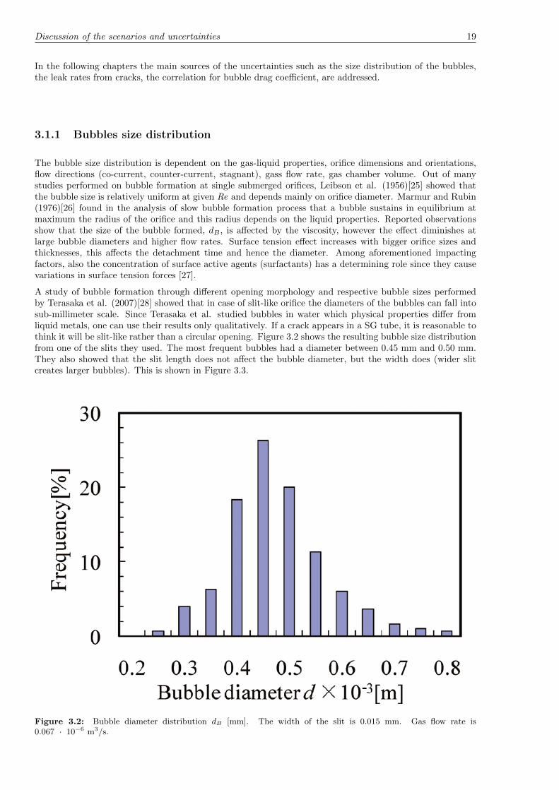
A study of bubble formation through different opening morphology and respective bubble sizes performedby Terasaka et al. (2007)[28] showed that in case of slit-like orifice the diameters of the bubbles can fall intosub-millimeter scale. Since Terasaka et al. studied bubbles in water which physical properties differ fromliquid metals, one can use their results only qualitatively. If a crack appears in a SG tube, it is reasonable tothink it will be slit-like rather than a circular opening. Figure 3.2 shows the resulting bubble size distributionfrom one of the slits they used. The most frequent bubbles had a diameter between 0.45 mm and 0.50 mm.They also showed that the slit length does not affect the bubble diameter, but the width does (wider slitcreates larger bubbles). This is shown in Figure 3.3.
Figure 3.2: Bubble diameter distribution dB [mm]. The width of the slit is 0.015 mm. Gas flow rate is0.067 · 10−6 m3/s.

20 Analysis of a steam bubble transport in the primary system of a pool-type LFR design
Figure 3.3: Effect of slit dimensions on bubble diameter. Gas flow rate is 0.83 · 10−6 m3/s.
Experimental data for bubbles formed into lead is very scarce. Together with uncertainties in the cracklocation, properties and flow field at that location, it is impossible to provide fully validated analysis for thebubble size distribution. Beznosov et al. (2005)[29] studied a process when water with pressure of 22–24MPa and temperature of 150–250 ◦C was pumped through a 10.0 mm diameter opening into liquid lead attemperatures 500–600 ◦C. The minimum radius they detected was 0.5 mm which is corresponding to thehighest resolution of the measurement system. According to their results, the most probable bubble radiusis around 1 mm. The measured distribution of vapor bubble radius is shown in Figure 3.4.
Figure 3.4: Vapor bubble size distribution.
According to the results of the above mentioned studies, we have chosen bubbles with diameters of 0.2 mm,0.4 mm, 0.5 mm, 1.0 mm, 2.0 mm, 4.0 mm and 6.0mm to be considered as possible realistic bubble sizes.
3.1.2 Leak rate
Among other factors, also the gas flow rate through the leak is determining the size of the appearing bubbles.Leakage flow rate, in turn, depends on morphology, area and geometry of the crack and the driving pressuredifference between two sides [30], [3]. In systems where heavy liquid metal, especially lead and lead-bismuth,is circulating, so called leak before break (LBB) is important due to possible slow corrosion and degradationof the SG tube wall. We assume that hard-detectable failures, mainly small cracks due to corrosion andstresses are the most dangerous. Critical chocked flow phenomena in case of a large opening (rupture of SG
Selection of the bubble drag coefficient correlation in liquid lead 21
tube) is not considered in this work.
To explain SG tube leakage and rupture phenomena further, it is useful to present studies performed byHwang et al. [3], [31] and [32]. These studies were initiated due to a plant outage in a Korean light waternuclear power plant where SG tube leaks were reported. Because cracks in highly corrosive environment candevelop already at relatively low stresses (high pressure difference is not necessary), even 100% through-wallcracks are found not to be a sufficient criterion for detectable leakage at normal operation conditions of PWR[3]. Therefore, it is expected that cracked tubes at operating pressure of 10.8 MPa will not show any leakage.Depending on the morphology of the opening (crack), first leaks were detected at pressures around 17 MPato 25 MPa (which is characteristic range of pressure difference in pool-type LFR). The corresponding flowrates were from 0.005 l/min (at 23.4 MPa) to 0.25 l/min (at 31.7 MPa). As a conclusion of all experimentsperformed by Hwang et al.(2004; 2005; 2008), including a series of burst rupture tests, the leak rates startfrom almost zero (initial state of the crack), develop up to several liters per minute after some time and canhave the maximum rate of 30-50 L/min (choke of the flow becomes the limiting factor).
For lead-cooled systems it is important to assess the impacts of small leak rates to the system, since they aredifficult to detect. In case of accumulation of smaller amounts of steam void takes place in the core, criticalsafety limits can be still tackled (and exceeded).
3.2 Selection of the bubble drag coefficient correlation in liquidlead
For validation of the approach, it is crucial to demonstrate that numerical solution obtained with selected dragcoefficient can reproduce experimentally observed terminal rise velocities for different bubble diameters. Thissection discusses the selection of a correlation for a steam bubble drag coefficient. For that purpose, terminalrise velocity of a steam bubble in steady liquid lead column is calculated with different drag correlationsdeveloped in the past. Then the predicted velocity is compared with analytically developed solutions andalso with available experimental data on a terminal rise velocity of a bubble in heavy liquid metals.
3.2.1 Bubble shape and rise behavior regimes
We begin with a theoretical description of the bubble shapes and motion in a quiescent viscous liquid.Dynamics of a bubble motion can be affected by many factors such as temperature, viscosity, pressure,purity of the surrounding fluid. Different regions of the bubble size, shape and the respective verticalupwards motion behavior are generally defined. The different properties and behavior of different bubblesmakes the realistic bubble size distribution in the system a very important part of the study. An overviewof the studies investigating bubble formation, sizes and rise velocities in water and in higher viscosity fluids(unfortunately not molten metals) is extensively presented in paper by Kulkarni and Joshi (2005) [27] andYang et al. (2007) [33]. Further into the theory behind the bubbles, drops and particles is explained in abook written by Clift et al. (1978) [34].
Therefore, prediction of terminal rise velocity is not a trivial task, especially taking into account a non-linearbehavior of drag coefficient, which dependents on the size and the shape of the bubbles. Different regimes,that govern the bubble motion in a continuous liquid with respect to different inter-facial shear (or drag) andresulting terminal velocity, can be defined as done by Maneri and Vassallo (2000) [35]:
• Spherical - dB < 0.25 mmIn this region viscous forces dominate and their shape is relatively spherical. The terminal rise velocityis well described by Stokes’ law (bubble velocity is proportional to the square of the diameter). Flowaround the bubble is smooth, streamlines reattach fully after the bubble, no separation occurs.
• Ellipsoidal - 0.25 mm < dB < 1.0 mmIn this region, with increasing bubble volume, the pressure on the front side increases which flattensthe bubble in the direction of motion.The rise velocity reaches the peak of about 20 cm/s (depends onthe gas and fluid of course) after which the smooth streamlines are destroyed and turbulent wake isformed. This wake grows with the bubble diameter and results in gradual decrease in terminal velocity.Nevertheless, this turbulent wake reattaches downstream rather steadily .
• Ellipsoidal (oscillatory) - 1.0 mm < dB < 2.5 mmWhen bubble diameter exceeds 1.0 mm, the vortexes behind the bubble do not reattach in a steady

22 Analysis of a steam bubble transport in the primary system of a pool-type LFR design
manner any longer – inwards rolling eddies produce oscillation. Bubble shape stretches out alternatelyin width and in motion direction. This elongation or compression in the vertical direction can beexplained by the varying pressure field below the bubble due to varying vortex field.
• Ellipsoidal (wobbly) - 2.5 mm < dB < 5.0 mmBubble size is large enough to be effectively affected by the surface tension forces present in the liquidfilm between the bubble sides and the wall of the injecting slit/crack/opening. This causes initialperturbation. The bubble starts to oscillate, wobble, stretch and distort about a planar ellipticalshape as rising. Now, after reaching the lowest rise velocity (happens in the mostly oscillating regime)increasing dB makes the buoyancy forces more dominating and the velocity starts to increase, again.
• Cylindrical cap - 5.0 mm < dB < 10.0 mmNow the bubble vertical cross section resembles a cap with flat bottom and spherical top. Top surface isrelatively stable, bottom may somewhat wobble and distort and cause vortex shedding. Inertial forcesare dominating from here on.
• Slug - dB < 10.0mm - The rise velocity approaches to a steady value around 18-19 cm/s and isindependent on the equivalent bubble diameter. The bubble is called slug when the horizontal cross-sectional area is larger than two-thirds of the test section area.
The resulting plot is shown in Figure 3.5. This brings qualitative but very broad insight to the relationsbetween terminal velocities (present in Re number) and shape regimes (Eo and Mo).
Figure 3.5: Shape regimes for bubbles and drops in unhindered gravitational motion through liquids.

Selection of the bubble drag coefficient correlation in liquid lead 23
The dimensionless groups, the Reynolds number (Re), the Etvs number (Eo) and the Morton number (Mo)are often used to describe the shape of a bubble and its rise behavior
Re =ρlubdbµl
(3.1)
Eo =g∆ρdb
2
σ(3.2)
Mo =g∆ρµl
4
ρ2l σ3
(3.3)
3.2.2 Modeling bubble motion in a column of liquid lead
In this work, I have used the Lagrangian model for bubble transport in a continuum flow field of liquidlead. For the task of validation of bubble drag correlation, a lead column of 0.5 m x 0.5 m x 5 m, wasmodeled. It was built using 3D-Cad software existing in Star-CCM+ package. The top and the bottomsurfaces of the column were defined as walls and particle interaction type was escape” there. The sidewallsof the column were defined as symmetry planes with “rebound” option for particles. The geometry can beseen in Figure 3.6. Both, the surface and the volume were meshed using internal mesher of Star-CCM+.Column geometry consists of 86 444 vertices, 23 826 cells and 116 788 faces.
Figure 3.6: Column geometry used for bubble model analysis.
Liquid lead material properties were defined in Star-CCM+ according to the recommended correlations formain thermo-physical properties [36]. All the values are based on reference temperature of 750 K (476.85◦C),which is in the range of operating temperatures of ELSY coolant (core inlet and outlet temperatures 400◦Cand480◦C, respectively). All defined material values are presented in Table 3.1.

24 Analysis of a steam bubble transport in the primary system of a pool-type LFR design
Table 3.1: Liquid lead properties
Parameter Value Parameter ValueTref (K) 750.00 Tboil (K) 2016.00Density (kg/m3) 10 471.2 Psat (Pa) 8.46·10−4
Thermal expansion coefficient (1/K) 1.14·10−4 Tsat (K) 2016.00Specific heat (J/kg·K) 145.5 Qvaporization (J/kg) 858 200Mol. viscosity (N·s/m2) 0.00124 Surface tension (N/m) 0.43425Therm. cond. (W/m·K) 17.45 Mol. weight (g/mol) 207.2Tcritical (K) 4870 Speed of sound (m/s) 1 737.97Pcritical (MPa) 100
Lead flow field, through which bubbles are transported, is described as a space with specified formulations init, called continuum. The physics continuum is a continuous phase whose governing equations are expressedin Eulerian frame of reference. In Star-CCM+, the continuum is a collection of models that representsthe substance (fluid or solid) being simulated [37]. Bubbles were assumed to be incompressible; their size(density) was not a function of pressure. Density and viscosity of the bubble gas was assumed equal to watervapor density at 100◦C under atmospheric pressure.
For modeling stagnant flow without turbulence, the steady state solution was imposed as initial condition.All the solvers for flow parameters were turned off, only Lagrangian Steady State solver is now active. Leadflow velocity was set to zero and temperature was 450◦C. Models chosen for this (liquid Pb) continuum, werefollowing:
• Constant density
• Gravity
• Segregated flow
• Segregated Fluid Temperature
• Steady
• Three dimensional
• Laminar
• Liquid
– Lead
• Lagrangian Multiphase
– Water vapor
In a reactor simulation, it is important to account the effect of turbulence, since it allows bubbles to “jump”from one “averaged” streamline to another. Without the effect of turbulence, the bubbles will always followthe same streamline, which is physically unreasonable for a turbulent flow. Set of used models for turbulenceis following:
• Constant density
• Gravity
• K-Epsilon turbulence
• Reynolds-Averaged Navier-Stokes
• Segregated flow
• Segregated Fluid Temperature
• Steady

Selection of the bubble drag coefficient correlation in liquid lead 25
• Three dimensional
• Turbulent
• Two-Layer All y+ Wall Treatment
• Liquid
– Lead
• Lagrangian Multiphase
– Water vapor
– Turbulent dispersion
So-called random-walk technique[20] is employed in turbulent dispersion model of Lagrangian phase to sim-ulate the fluctuating velocity field. A bubble is assumed to be affected by a sequence of eddies as it travelsthrough the turbulent flow field. Every eddy causes a local disturbance to the Reynolds-averaged velocityfield
v = v + v′ (3.4)
where v is the local Reynolds-averaged velocity and v′, is the eddy velocity fluctuation, unique to eachparticle. The magnitude of the fluctuation is random at each time instant and has a normal (Gaussian)distribution with zero mean value and a standard deviation given by eddy velocity scale, which is describedby the following formula
ue =ltτt
√2
3=
√2
3k (3.5)
where lt and τt are the length-scale and time-scale of the turbulence and k is turbulent kinetic energy providedby the turbulence model (k-epsilon used here) [37]. In present case, the value for turbulent kinetic energywas 0.1 J, which corresponds to eddy velocity fluctuation of about 0.25 m/s. No average flow was actuallymodeled in this case. One can envisage a situation when a steady pool is stirred to introduce eddies withconstant energy while the averaged flow is zero through the pool.
Terminal velocity of rising bubble in laminar stagnant column was detected as the bubble velocity at thecolumn outlet. In case of turbulent stagnant flow the terminal rise velocity was calculated based on thecolumn height and particles residence time.
3.2.3 Drag coefficient correlations
In 1992, Karamanev and Nikolov [38] experimentally showed that the trajectories of rising bubbles do differfrom the ones of free falling spherical particles. Also the terminal rise velocity was shown to be smaller incase of rising bubbles. Since, it was realized that in addition to skin drag (which is affected by internalcirculations too), there is so called form drag present in case of non-rigid bubbles (different shape regionsdescribed in earlier chapter). This makes the whole drag formulation for bubbles more complex. Productionof the drag force that tends to slow down the relative motion of a bubble is one of the most important effectsof viscosity on the displacement of the bubble in a liquid. The drag force is essentially a balance between thework done by the drag force and the viscous dissipation within the fluid environment and can be formulatedas
Fd =CdρvT
2A
2(3.6)
where Cd is the balancing (proportionality) constant (or drag coefficient) and can have different forms de-pending on Re number, systems’ physicochemical properties of the liquid and the bubble dimensions. vTis the terminal relative velocity between two phases and A is the cross-sectional area. One of the widestoverview for the drag coefficient and different correlations of the last, is performed by Kulkarni and Joshi(2005) [27].
The drag coefficient, Cd, has a determining influence on the bubble terminal rise velocity. Cd in turn is afunction of Re in most cases (the effect decreases with low Re). The complexity of estimation of Cd as well asRe is due to the time-dependent viscosity and its effect on the bubble shape. Since it is not straightforwardto obtain the rise velocities directly, one aims to develop correlations for one of its variants (viz. Cd, Re).In this thesis, I have tackled the uncertainty reduction in bubble terminal rise velocity by choosing the dragcorrelation that fits the best with both, existing data and analytical solutions.

26 Analysis of a steam bubble transport in the primary system of a pool-type LFR design
There are four different drag coefficient correlations in the analysis. Star-CCM+ provides two general methodsfor defining the drag coefficient:
• Schiller-Naumann correlation
• User-Defined Field Function (UDF)
Firstly, the only correlation implemented in Star-CCM+, Schiller-Naumann correlation, is used. This cor-relation is suitable for spherical solid particles and small diameter bubbles (as it is defined in [37]). It isformulated as:
Cd =
24
ReB(1 + 0.15Re0.687B ), ReB ≤ 103
0.44, ReB > 103(3.7)
The dispersed phase (bubble) Reynolds number is defined as:
ReB =ρc|vr|dB
µc(3.8)
where ρc and µc are the density and the dynamic viscosity of the continuous phase (lead) respectively, vr isthe relative velocity between the bubble and lead, and dB is spherical bubble diameter.
Secondly, Schiller-Naumann coefficient correlation with modification in the low Reynolds number regionaccording to Stokes law was used [39]. This was implemented using a User-Defined Field Function. It has aform of:
Cd =
24
ReB
2 + 3µd
µc
3 + 3µd
µc
ReB ≤ 2
24
ReB(1 + 0.15Re0.687B ), 2 < ReB ≤ 103
0.44, ReB > 103
(3.9)
where µd is the dynamic viscosity if the dispersed phase (steam bubble).
Thirdly, a correlation proposed by Rodrigue [40] was used:
Cd =16
ReB
(0.5 + 32Θ + 0.5
√1 + 128Θ)1/3
+ (0.5 + 32Θ− 0.5√
1 + 128Θ)1/3
+ 0.036(128
3
1/9
)Re8/9B Mo1/9
9/4
(3.10)
where Θ = (0.018)3( 23 )1/3)ReB
(8/3)Mo(1/3).
Fourth correlation used in this work was developed by Tomiyama et al. [41]:
Cd = max
{min
[16
ReB(1 + 0.15Re0.687B ),
48
ReB
],
8
3
Eo
Eo+ 4
}(3.11)
This general correlation fits well with available experimental data.
3.2.4 An approach to verification of modeling method
Since there is no available experimental data on bubble terminal rise velocity in lead, the simulation resultswere compared to Stokes law that predicts velocity for small, spherical shape bubbles and to Mendelsonsequation that predicts velocities in surface tension- and inertia-dominated regimes [42]. Comparison of Stokeslaw and Mendelson equation with experimental data for bubble terminal rise velocity in mercury obtainedby Mori et al. [43] is shown in Figure 3.7. As it can be seen, the bubble velocity is predicted reasonably wellby Mendelsons equation in the surface tension and buoyancy dominated regime. Small bubbles are expectedto behave as solid spheres and their terminal velocity is described by Stokes law. This agreement provides usa reference against which we are validating the results obtained with different drag coefficient correlations.

Selection of the bubble drag coefficient correlation in liquid lead 27
0 1 2 3 4 5 6 7 8 9 100
0.1
0.2
0.3
0.4
0.5
0.6
bubble diameter [mm]
velo
city
[m/s
]
Stokes lawMendelsons eq. for PbMori et al. data for Hg
Figure 3.7: Bubble terminal rise velocity vs. bubble diameter. Analytical predictions by Stokes and Mendelsonslaws. Experimental data for velocities in Hg.
3.2.5 Results of verification
Four different drag coefficient correlations discussed in previous system were tested. First calculations wereperformed without activating turbulent dispersion model for particles. Figure 3.8 presents the terminal risevelocities obtained using different drag correlations. It can be seen that Schiller-Naumann correlation isapplicable only for very small bubbles (which behave as they were rigid spheres). The modified Schiller-Naumann correlation does not improve the prediction. Rodrigues correlation shows a better agreement thanSchiller-Naumann, but is still deficient in capturing the peak in the curve. Tomiyamas drag correlation, whichaims to match the whole drag curve, provides the best agreement with the Stokes solution and Mendelsonequation for bubble rise velocities. Therefore, Tomiyamas correlation was used in following study of bubbletransport in reactor conditions.
0 1 2 3 4 5 6 7 8 9 100
0.1
0.2
0.3
0.4
0.5
0.6
bubble diameter [mm]
velo
city
[m/s
]
Stokes lawMendelson eq.Schiller−NaumannModif. Schiller−NaumannRodrigueTomiyama et al.
Figure 3.8: Bubble terminal rise velocities calcuated with different drag coefficient correlations.

28 Analysis of a steam bubble transport in the primary system of a pool-type LFR design
2 4 6 8
0.1
0.2
0.3
0.4
bubble diameter [mm]
velo
city
[m/s
]
Without turb. dispersionWith turb. dispersion
Figure 3.9: Bubble terminal rise velocity vs. bubble diameter. Results obtained with and without modelingturbulent dispersion of a bubble.
A comparison between the results obtained with and without turbulent particle dispersion modeling wasdone for Tomiyamas correlation. As it appears in Figure 3.9, a difference between terminal rising velocityof a bubble in laminar and in turbulent lead column is negligible as it is expected in isotropic homogeneousturbulent flow field.
3.3 Bubble transport to the ELSY core in case of SGTL
In this section we address the possibility of bubble transport from the steam generator to the core regionin the ELSY LFR design. First a brief overview of the preliminary configuration of ELSY design and itsnominal full power operation parameters are presented. Then the averaged steady state full power operationflow is resolved in a realistic model of the ELSY primary system. Injector features in Star-CCM+ are usedto initiate bubbles in the system. The behavior of individual bubbles in the obtained steady state flow fieldwill be calculated using Lagrangian specification, taking into account dispersion of the bubbles by turbulentvortexes. The results are containing estimation of the probability that a bubble of certain size and injectedat a certain location in the SG can reach the core region is given.
3.3.1 ELSY reactor design
Geometry
The primary system of ELSY design comprises of a circular reactor vessel that accommodates all the internalswhich are used for safe heat transfer from the core via moving liquid lead to the water as working fluid in thesecondary system. The vessel is a pool that has a fixed roof (large annular steel plate) and a half-sphericalbottom head. The volume between the primary coolant free level and the reactor roof is filled by a cover gasplenum. Reactor core is submerged in the middle part of the pool and surrounded by 8 steam generatorsin direct contact with molten lead, located at the top part of the pool. To fit all required components,the outline dimensions are: vessel outside diameter of 12.3 m by 8.65 m of height. The ELSY referenceconfiguration can be seen in Figure 3.10 [44].

Bubble transport to the ELSY core in case of SGTL 29
Figure 3.10: ELSY reactor reference configuration [44].
SG in lead-cooled systems provides heat removal from low-pressure heavy liquid metal on the primary side tothe high-pressure water/steam flow on the secondary side. The preliminary configuration of ELSY foresees8 Steam Generator Units (SGU) (see Figure 3.11), each of them characterized by spiral-wound tube bundlehoused in the bottom-closed, annular space with vertical inner and outer permeable shells. The inlet ofeach tube is connected to the feed water header and the outlet is connected to the steam header. EachSG has a coaxial flow pump in it which provides the head required to force the coolant radially throughperforated inner shell, past heat exchanger tube bundles, through the outer shell. Effectively this schemeis a counter-current heat transfer since the feed water in tubes circulates from outer spiral to inner spiral(Figure 3.12).
Figure 3.11: Scheme of the primary pump - steam generator unit [45].

30 Analysis of a steam bubble transport in the primary system of a pool-type LFR design
Figure 3.12: Tubes - headers connections. Upper header is attached to the feed water line and the lower one to thesteam line [45].
Operational parameters
The pool-type ELSY fast reactor, used as a reference case here, has electrical power of 600 MW [45]. Thermalefficiency is about 40%. The nominal operational parameters that are considered in the preliminary ELSYconfiguration for the steady state flow are following:
Table 3.2: Initial tentative parameters of ELSY plant [45], [46], [47].
Parameter ValueMass flow 16.05 ton/s/SGCore inlet temperature 400◦CCore inlet temperature 480◦CCore pressure drop 0.9 bar,Steam generator pressure drop 0.3 barTotal primary pressure drop 1.4 bar
3.3.2 Modeling of primary system at nominal operational conditions
The simulation domain represents 1/8th slice of the ELSY reactor vessel, comprising one SG including hotleg and pump and a slice of the core region together with corresponding parts of the hot/cold plenum anddowncomer.
The parameters that were presented in the previous section were used to determine a set of boundaryconditions and uniformly distributed heat source term in the core region, heat sink term in the steamgenerator region and momentum source term in the pump region (see Figure 3.13), which are presented inTable 3.3.

Bubble transport to the ELSY core in case of SGTL 31
Table 3.3: Defined source terms per region.
Region Kq[kg/m4] Q[W/m3] Porosity Mom. source [N/m3]
Core 112635 9.2 · 107 0.5 -
Steam generator 1.25 · 107 T−335◦C145◦C · −187.5MW
VSG0.65 -
Upper/lower plenum 112635 - 0.6 -
Pump 74093 - 0.9 540 000
Shielding 2.2527 · 107 - 0.9 -
A source of momentum in the pump was adjusted together with quadratic resistance coefficients in the core,SG, upper/lower plena and shielding regions, to obtain design mass flow rate. Heat sink expression, asdescribed in Table 3.3, assured that the lead temperature at the SG inlet was 480◦C. If the temperaturewas lower or higher than design temperature, then less or more heat was removed respectively in the steamgenerator. In total, 9 regions were defined in the simulation domain. All the solid boundaries in the designare modeled as adiabatic, no-slip walls. Left and right side of the simulation domain are defined as symmetryplanes. And free surfaces (hot and cold) are defined as adiabatic, slip walls.
Modeling flow physics
Firstly, to obtain design based operational steady state flow field, a physics continuum was defined, whichcontains the collection of all models that represent the simulated substance (liquid lead and steam particles).For mass, momentum and energy equations the coupled implicit solver was used. Density was modeledas constant (Boussinesq model is invoked when this option is chosen together with gravity, meaning thatvariation in density due to temperature is still taken account in gravity term in momentum equation by theuse of thermal expansion coefficient). Choice for the turbulence modeling was the RANS realizable k − εmodel, using a two-layer all−y+ formulation [37].
Modeling and meshing ELSY geometry
The geometry, used in the simulations, was extracted as boundary surface from initial volume mesh whichwas created with Pointwise Gridgen by our colleague Carlsson in JRC [48]. The new mesh was created withStar-CCM+ internal mesher.
The mesh used in the calculation consists of 679 480 polyhedral cells. Target characteristic size of a cell inthe domain was 0.07 m. We used 5 layers of prism cells for the modeling of boundary layers on the solidwalls. The total thickness of the prismatic cell layer was 0.02 m and smallest prism cell height near the wallwas 0.0015 m and the wall y+values were mostly below 100. The 3D volume mesh (with distinct regions)and the mesh on a vertical cross-section is shown in Figure 3.13.

32 Analysis of a steam bubble transport in the primary system of a pool-type LFR design
Figure 3.13: 3D volume mesh and a vertical cross-section of it.
Steady state flow results
A satisfactory steady state was achieved at nominal mass flow rate of 16.09 ton/s and area averaged tem-peratures at core inlet 402.7◦C and core outlet 485.3◦C, which gives an average temperature rise in the core82.6◦C. The predicted pressure drop over the core was 0.85 bars and 0.29 bars in the SG. Total pressure dropof 1.6 bars was calculated for the whole primary system. Coolant temperature distribution in the verticalcross-section plane is shown in Figure 3.14. Analysis of the velocity vector field presented in Figure 3.15suggests that there is a region with relatively high downward speed of the coolant flow near the vessel wall inthe downcomer. As we will show in the next section such flow is sufficient for dragging steam bubbles fromthe SG to the core region.
Figure 3.14: Temperature field during normal operation.
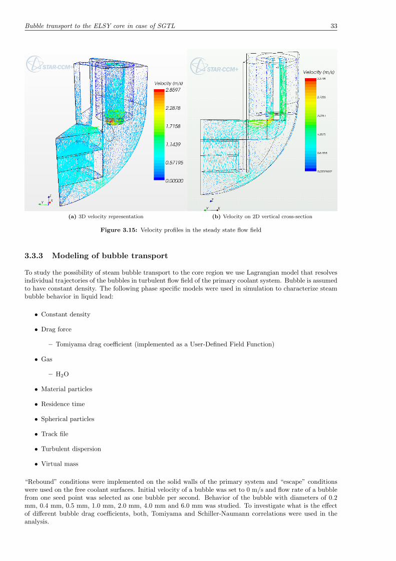
Bubble transport to the ELSY core in case of SGTL 33
(a) 3D velocity representation (b) Velocity on 2D vertical cross-section
Figure 3.15: Velocity profiles in the steady state flow field
3.3.3 Modeling of bubble transport
To study the possibility of steam bubble transport to the core region we use Lagrangian model that resolvesindividual trajectories of the bubbles in turbulent flow field of the primary coolant system. Bubble is assumedto have constant density. The following phase specific models were used in simulation to characterize steambubble behavior in liquid lead:
• Constant density
• Drag force
– Tomiyama drag coefficient (implemented as a User-Defined Field Function)
• Gas
– H2O
• Material particles
• Residence time
• Spherical particles
• Track file
• Turbulent dispersion
• Virtual mass
“Rebound” conditions were implemented on the solid walls of the primary system and “escape” conditionswere used on the free coolant surfaces. Initial velocity of a bubble was set to 0 m/s and flow rate of a bubblefrom one seed point was selected as one bubble per second. Behavior of the bubble with diameters of 0.2mm, 0.4 mm, 0.5 mm, 1.0 mm, 2.0 mm, 4.0 mm and 6.0 mm was studied. To investigate what is the effectof different bubble drag coefficients, both, Tomiyama and Schiller-Naumann correlations were used in theanalysis.

34 Analysis of a steam bubble transport in the primary system of a pool-type LFR design
Injectors
In Star-CCM+, injectors are used to define the location, direction, rate at which the bubbles enter the fluidcontinuum and the velocity of an entering bubble. Also the flow rate distribution type (rate per injectionpoint or the total rate), flow rate specification type (particle, mass or volume flow rate) and particle sizespecification type (diameter or mass) are defined by injector. Particle diameter, in turn, can be definedas: a) constant; b) by a specific size distribution (Log-Normal, Rosin-Rammler) or c) by User-Defined FieldFunction. In the main core of the analysis particle diameters are set to a constant value and changed manuallybetween discrete values that are of interest in SGTL. In one case we used an UDF according to Eq. 3.12 tosee how much the results are affected by the change of particle diameter due to changing hydrostatic pressurewhile traveling in the domain.
dB(Pdepth) = 3
√P0
Pdepth· dB0
(3.12)
where P0 is atmospheric pressure, Pdepth is the hydrostatic pressure at the depth of a bubble and dB0is the
bubble diameter at atmospheric conditions.
Figure 3.16: Locations of the planes used as bubble injectors in SG. (Color bar legend shows the vertical upwardvelocity of the lead at these planes).
The SG leakage was simulated by injecting bubbles at three different levels (see Figure 3.16) in the SG 5.2m, 6.87 m and 8.55 m from the bottom of the pool (the total depth of the pool is 8.65 m). All these injectorsare by type spherical planes belonging to SG region only. These particular heights are selected to simulatethe SG tube leakage happening in the bottom, center and upper part of the SG. Each plane contains all meshcells at this height inside SG, whereas each of those cells can be an injection point.
There were also two other injection locations used according to the requirements set by the method we usedfor estimation of the void accumulation rates (see Section 3.3.4). One of them is situated close to the exit ofthe core and the other in the vicinity of the pump outlet. They are shown in Figure 3.17.
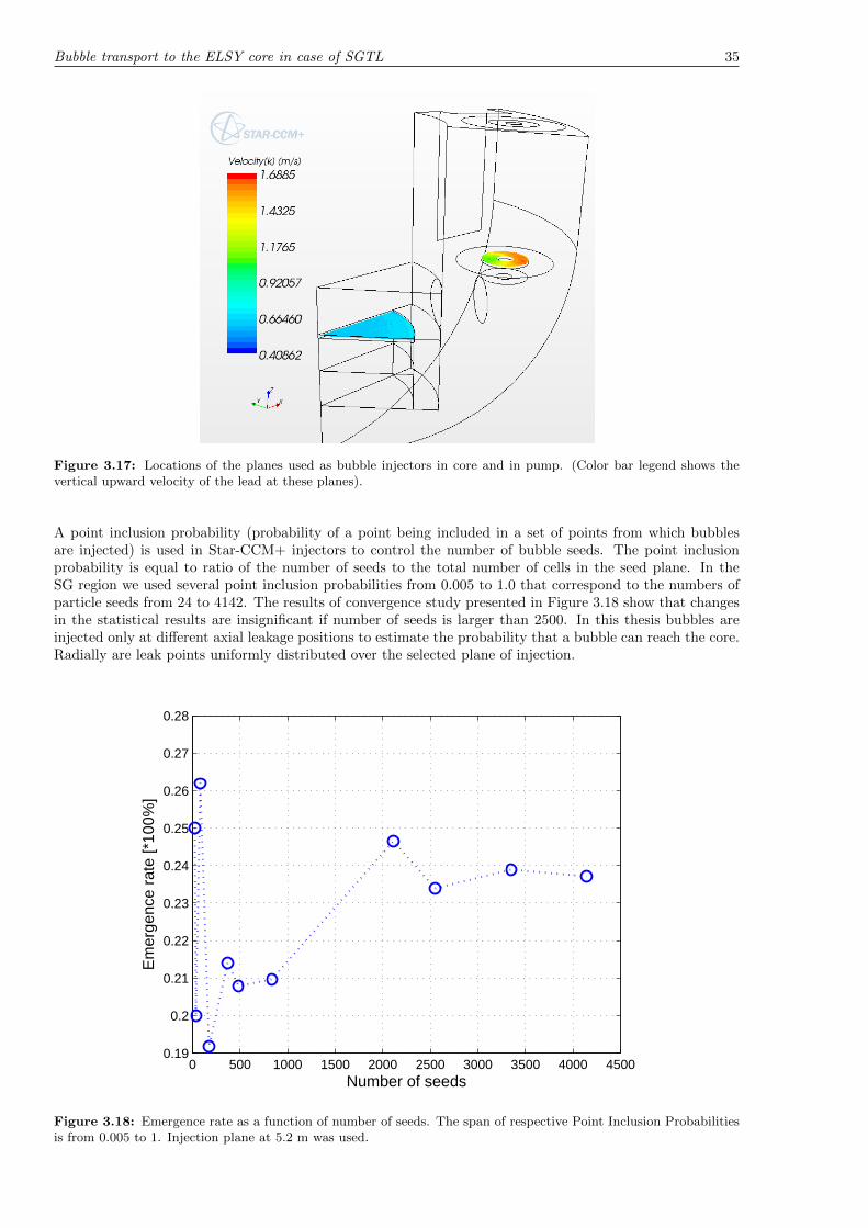
Bubble transport to the ELSY core in case of SGTL 35
Figure 3.17: Locations of the planes used as bubble injectors in core and in pump. (Color bar legend shows thevertical upward velocity of the lead at these planes).
A point inclusion probability (probability of a point being included in a set of points from which bubblesare injected) is used in Star-CCM+ injectors to control the number of bubble seeds. The point inclusionprobability is equal to ratio of the number of seeds to the total number of cells in the seed plane. In theSG region we used several point inclusion probabilities from 0.005 to 1.0 that correspond to the numbers ofparticle seeds from 24 to 4142. The results of convergence study presented in Figure 3.18 show that changesin the statistical results are insignificant if number of seeds is larger than 2500. In this thesis bubbles areinjected only at different axial leakage positions to estimate the probability that a bubble can reach the core.Radially are leak points uniformly distributed over the selected plane of injection.
0 500 1000 1500 2000 2500 3000 3500 4000 45000.19
0.2
0.21
0.22
0.23
0.24
0.25
0.26
0.27
0.28
Number of seeds
Em
erge
nce
rate
[*10
0%]
Figure 3.18: Emergence rate as a function of number of seeds. The span of respective Point Inclusion Probabilitiesis from 0.005 to 1. Injection plane at 5.2 m was used.

36 Analysis of a steam bubble transport in the primary system of a pool-type LFR design
3.3.4 Strategy for estimation of core voiding
In general, the quantification of the probability that a bubble of certain size can reach the core region iscalculated by dividing the number of bubbles that reached the core by the total number of bubbles releasedin a particular location (region of injection points) in SG. The bubbles are injected at three height levelsinside the SG.
The following three-step method is used in assessment of void accumulation rate in the core. The bubblesinjected through the crack in SGT into the primary coolant flow have generally three possibilities (dependingon their size, leak location and flow characteristics) to escape the system (see Figure 3.19):
1. They escape after injection immediately to the cold free surface above the downcomer and the SG.
2. They are dragged to the core for the first time and escape from the loop to the hot free surface abovethe core.
3. They stay in the primary coolant flow until they travel through the pump and reach the SG again andemerge to the cold free surface this time.
All the bubbles which do not escape the system at any of those steps, are considered to be carried continuouslyby the coolant flow through the primary loop. Having obtained valid probabilities to reach the core fordifferent size bubbles and different injection locations, is the starting point for assessment of the SGTLconsequences according to different scenarios of void behavior (see the first section in this chapter for scenariodefinitions).
Figure 3.19: Different locations where the probabilities for a bubble to escape the primary loop are estimated (1-3).P1-P3 are defined at these locations as the probabilities for a bubble to stay in the loop.
Here is a more detailed explanation on how to calculate the probabilities related to aforementioned ways ofescape with respect to different injection locations.
First, all bubbles are injected at one of the three injection levels in the SG. The injection rate per all injectionpoint in total has set to a constant value of one bubble per second. We can estimate the probabilities that

Bubble transport to the ELSY core in case of SGTL 37
a bubble will stay in the loop or will escape from the primary system by counting the number of bubblesthat reach the lower plenum and the number of those that escape through the cold free surface during thegiven residence time and relating them to the total number of bubbles injected during the same time. E.g.if 50% of the bubbles reach the lower plenum and 50% reach the cold free surface in the downcomer region,then the measured particle flow rate at both of them is 0.5 1/s. Now, after the liquid lead steady stateflow field has been calculated, the solvers for flow will be switched off by setting the number of cycles ofalgebraic multi-grid solver to 0. Only the trajectories of Lagrangian particles (with necessary parametersfor them) are calculated. This enables us to catch and count the bubbles that are entering the core (andthe reflector/dummy) region by changing the interface type at the bottom boundaries of lower plenum andreflector regions to baffle without affecting the flow field. Baffle is the only interface type on which theboundary condition for Lagrangian phase can be set to “escape”. This saves calculation time and moreimportantly, allowing to count the particles entering the core only once (they do not influence the results bygoing through the whole primary system and re-enter the core again) while keeping the maximum residencetime of particles sufficiently high, so the maximum number of bubbles will either escape to the core or emergeto the free surface. Bubbles that entered the core and reflector regions are counted at the inlet boundaries ofthese regions. The fraction of those to total number of bubbles is P1 – measure of probability that bubblesinjected in SG can reach the core.
Now we proceed to estimation of the second probability, P2. This step is in principal done only for the bubblesthat have already traveled through the core. The bubbles are injected at the horizontal plane slightly belowthe outlet of the core. The bubbles that will escape from the simulation domain to the hot free surface (theliquid lead surface above the core region) are counted. P2 is one minus the fraction of those bubbles to thetotal bubbles injected at the top of the core, namely the ones that are moving with the coolant flow backtowards the steam generator.
Finally, to assess the fraction of bubbles that will stay in the primary loop even after the third stage, havingjust passed through the pump, the bubbles are injected close to the exit of the pump and those that reachthe core inlet are counted. This is defined as probability P3.
Having these three probabilities, one can estimate the probability that a bubble can reach the core in thefirst place and also make an assessment about the the total probability for a bubble to stay in the primaryloop and therefore contribute to the accumulation of the void in the core. The accumulation rate dependson three parameters: 1) steam injection flow rate; 2) actual bubble size distribution of injected bubbles; 3)probability that bubbles of each size can stay in the primary loop. This can be expressed as follows:
Qprimary(t) = Qleak(t)
N∑i=1
fdi · P1di · P2di · P3di (3.13)
where Qprimary(t) is the rate of accumulation of void in the primary system, Qleak(t) is the volumetric leakrate [litres/day], fdi, P1di, P2di, P3di are volume fraction and respective probabilities for a bubble with sizedi, and N is the number of bubbles sizes considered in the bubble size distribution.
It is also interesting to estimate the void accumulation rate in the core (assuming that all bubbles that reachthe core will stay in the core, e.g. below spacers):
Qcore(t) = Qleak(t)
N∑i=1
fdi · P1di (3.14)
To estimate the realistic rate of void accumulation in the core one needs to consider the probability thatbubble will pass or stuck in the core given detailed geometry of the core internals. This task is beyond thescope of the present work.

38 Analysis of a steam bubble transport in the primary system of a pool-type LFR design
3.3.5 Results and discussion
Injection level 5.2 m
Trajectories of injected bubbles are shown below (Figures 3.20, 3.21, 3.22, 3.22, 3.23, 3.24, 3.25 and 3.26). Itcan be seen from these figures that small (0.2 mm and 0.4 mm in diameter) bubbles are dragged to the core,medium size (0.5 mm and 1.0 mm) bubbles escape the primary coolant system after certain residence timeand bigger bubbles (2.0 mm, 4.0 mm and 6.0 mm) again are more affected by the coolant flow and draggedto the core.
Figure 3.20: Injection height 5.2 m. Bubble diameter 0.2 mm.
Figure 3.21: Injection height 5.2 m. Bubble diameter 0.4 mm.

Bubble transport to the ELSY core in case of SGTL 39
Figure 3.22: Injection height 5.2 m. Bubble diameter 0.5 mm.
Figure 3.23: Injection height 5.2 m. Bubble diameter 1.0 mm.
Figure 3.24: Injection height 5.2 m. Bubble diameter 2.0 mm.
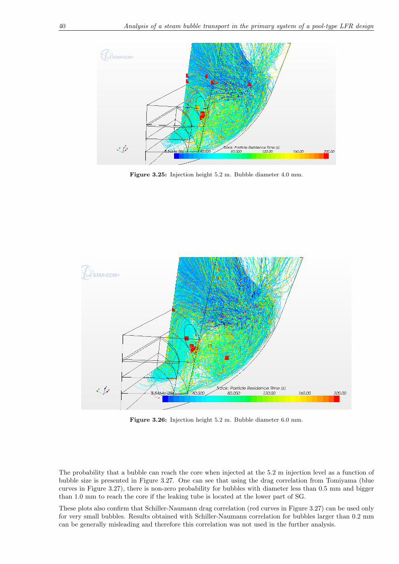
40 Analysis of a steam bubble transport in the primary system of a pool-type LFR design
Figure 3.25: Injection height 5.2 m. Bubble diameter 4.0 mm.
Figure 3.26: Injection height 5.2 m. Bubble diameter 6.0 mm.
The probability that a bubble can reach the core when injected at the 5.2 m injection level as a function ofbubble size is presented in Figure 3.27. One can see that using the drag correlation from Tomiyama (bluecurves in Figure 3.27), there is non-zero probability for bubbles with diameter less than 0.5 mm and biggerthan 1.0 mm to reach the core if the leaking tube is located at the lower part of SG.
These plots also confirm that Schiller-Naumann drag correlation (red curves in Figure 3.27) can be used onlyfor very small bubbles. Results obtained with Schiller-Naumann correlation for bubbles larger than 0.2 mmcan be generally misleading and therefore this correlation was not used in the further analysis.

Bubble transport to the ELSY core in case of SGTL 41
0 1 2 3 4 5 60
0.1
0.2
0.3
0.4
0.5
0.6
0.7
0.8
0.9
1
Bubble diameter [mm]
P1
− p
roba
bilit
y to
rea
ch th
e co
re a
fter
inje
ctio
n
TomiyamaSchiller−Naumann
Figure 3.27: Fraction of bubbles that reach the core inlet. Obtained with different drag correlations.
Figure 3.28 shows the probabilities that a bubble can reach the core inlet for simulations with constantbubble diameter and simulations where bubble diameter is a function of surrounding hydrostatic pressure.Two curves are exhibiting the same tendency, but are somewhat shifted. This shift can be explained bytwo facts: a) in case of pressure dependent bubble diameter we have chosen the free surface of lead as thereference altitude for diameter dB0 which means that the initial diameter of a bubble at location plane 5.2 mfrom the bottom ( 3.5 m hydrostatic head above it) is already about 1.5 times smaller and b) when a bubblemoves downward, its diameter decreases and it starts to behave as a smaller bubble. This moves the curverightwards.In this range of bubble diameters, according to Figure 3.28, the shifts are about half a millimeter. This canbe considered the within error of measurements of the bubble size distributions that we have used in thisanalysis since there are factors affecting bubble sizes that we have not taken into consideration in detail andwhich define the bubble sizes in real application (uncertainties in the crack morphology, pressure differencesin a particular accident scenario, bubble–hot lead interaction). Therefore the qualitative picture can becaptured well enough even with simulations with constant bubble diameters.
0 1 2 3 4 5 60
0.1
0.2
0.3
0.4
0.5
0.6
0.7
0.8
0.9
1
Bubble diameter [mm]
P1
− p
roba
bilit
y to
rea
ch th
e co
re a
fter
inje
ctio
n
constant d
B
dB=d
B(pressure)
Figure 3.28: Fraction of bubbles that are dragged to core.

42 Analysis of a steam bubble transport in the primary system of a pool-type LFR design
Figure 3.29 illustrates the probability P2 as a function of bubble diameter. One can see that there is asignificant fraction of bubbles which will escape to the hot free surface after passing through the core once(more than 50% of bubbles with diameter around 0.5 mm is removed). Nevertheless, the plot suggests thatmore than half of bubbles with diameter smaller than 0.5 mm and bigger than 1 mm will continue travelingin the system.
0 1 2 3 4 5 60
0.1
0.2
0.3
0.4
0.5
0.6
0.7
0.8
0.9
1
Bubble diameter [mm]
P2
− p
roba
bilit
y to
rea
ch th
e pu
mp
from
cor
e
Figure 3.29: Fraction of the bubbles that are carried through the core and further into the pump and SG.
Third escape possibility, however, seems to decrease the amount of void in the system significantly. Figure 3.30shows that except for very small (0.2 mm) bubbles, the probability to stay in the primary system after onecycle through the core is very low.
0 1 2 3 4 5 60
0.1
0.2
0.3
0.4
0.5
0.6
0.7
0.8
0.9
1
Bubble diameter [mm]
P3
− p
roba
bilit
y to
sta
y in
the
prim
ary
loop
afte
r on
e cy
cle
Figure 3.30: Fraction of bubbles that continue circulating in the primary loop.
According to the resulting probabilities that a bubble of certain size will stay in the primary loop we have

Bubble transport to the ELSY core in case of SGTL 43
estimated the void accumulation rate in the primary system. Analysis is done for two distinct cases and isbased on the procedure described in Section 3.3.4:
1. Assuming the size distribution of injected bubbles found by Sasaka and Terasada (2011) [28] and theminimum leak rate of about 0.005 L/min (7.2 L/day) (probable in the early stages after the SGTL).And the resulting accumulation rate of steam bubbles in the primary system is:
Q(t)small = Qleak(t)small · diSasaka&Terasaka· P1di · P2di · P3di = 0.012
L
day
2. Assuming the size distribution of injected bubbles found by Beznosov et al. (2005)[29] and the leakrate of about 0.25 L/min (360 L/day) (probable do develop upon some time after SGTL). And theresulting accumulation rate of steam bubbles in the primary system is:
Q(t)big = Qleak(t)big · diBeznosov· P1di · P2di · P3di = 0.85
L
day
Since there is uncertainty in the scenarios of how the void behaves in the primary system, we have analyzedalso a situation when bubbles are staying in the core (without passing it) due to getting stuck in vortexese.g. This means that we remove the probabilities which describe the bubble behavior after passing throughthe core, viz. P2di and P3di, from the accumulation rate expression. The void build-up values in the core ifthe bubbles would not leave it, are:
1. In case of smaller leakage:
Q(t)small = Qleak(t)small · diSasaka&Terasaka· P1di = 0.09
L
day
2. In case of bigger leakage:
Q(t)big = Qleak(t)big · diBeznosov· P1di = 96.44
L
day
Injection level 6.87 m
Trajectories of injected bubbles are shown below (Figures 3.31, 3.32, 3.33, 3.33, 3.34, 3.35, 3.36 and 3.37).
Figure 3.31: Injection height 6.87 m. Bubble diameter 0.2 mm.

44 Analysis of a steam bubble transport in the primary system of a pool-type LFR design
Figure 3.32: Injection height 6.87 m. Bubble diameter 0.4 mm.
Figure 3.33: Injection height 6.87 m. Bubble diameter 0.5 mm.
Figure 3.34: Injection height 6.87 m. Bubble diameter 1.0 mm.

Bubble transport to the ELSY core in case of SGTL 45
Figure 3.35: Injection height 6.87 m. Bubble diameter 2.0 mm.
Figure 3.36: Injection height 6.87 m. Bubble diameter 4.0 mm.
Figure 3.37: Injection height 6.87 m. Bubble diameter 6.0 mm.

46 Analysis of a steam bubble transport in the primary system of a pool-type LFR design
If the leak is located in the middle part of SG only very small (diameter less than 0.4 mm) bubbles can bedragged down to the core inlet (see the results in Figure 3.38). At this height level, both drag correlationsused suggest the same tendency.
0 1 2 3 4 5 60
0.1
0.2
0.3
0.4
0.5
0.6
0.7
0.8
0.9
1
Bubble diameter [mm]
P1
− p
roba
bilit
y to
rea
ch th
e co
re a
fter
inje
ctio
n
TomiyamaSchiller−Naumann
Figure 3.38: Fraction of the bubbles that reach the core inlet.
Here we used probabilities P2 and P3 that were presented in previous section. The void accumulation ratesin the system and in the core only, are:
1. In case of smaller leakage in the whole primary system:
Q(t)small = Qleak(t)small · diSasaka&Terasaka· P1di · P2di · P3di = 0.01
L
day
and in case of bigger leakage:
Q(t)big = Qleak(t)big · diBeznosov· P1di · P2di · P3di = 0.02
L
day
2. In case of smaller leakage in the core:
Q(t)small = Qleak(t)small · diSasaka&Terasaka· P1di = 0.02
L
day
and in case of bigger leakage:
Q(t)big = Qleak(t)big · diBeznosov· P1di = 0.03
L
day
It is instructive to mention that in each case the biggest contribution to the void comes from the smallest,0.2 mm, diameter size bubbles (as it can be seen from trajectory figures and probability plots as well).

Suggestions for mitigation of consequences of SGTL 47
Injection level 8.55 m
All bubbles injected at the topmost level (8.55 m) close to the cold free surface escape from the lead-pool.Therefore already P1 is zero and no threat is expected. We can already say that the higher location the SGtube leakage happens the smaller is the probability that a bubble can be dragged to the core. The trajectoriesof 0.2 mm and 1.0 mm bubbles that are injected at this height are presented in Figure 3.39 in Figure 3.40,respectively.
Figure 3.39: Injection height 8.55 m. Bubble diameter 0.2 mm. Point inclusion probability is 1.
Figure 3.40: Injection height 8.55 m. Bubble diameter 1.0 mm. Point inclusion probability is 0.01.
3.4 Suggestions for mitigation of consequences of SGTL
Significant fraction of the bubbles that can reach the core inlet in normal operation conditions suggest thatSGTL issue has to be considered in the design with adequate preventive and mitigative measures. First ofall, in case of SGTL (which seems to be likely), it is important to concentrate on the scenarios that mightpose the tendency to cause threat to the reactor. This means, to the scenarios in which the void actuallyreaches the core.
Therefore, one should definitely look into the design in order to have the flow path which prevents theappearance of so called local stagnation zones (corners) where bubbles can get stuck, accumulate and moveas bigger amount of void at a time into the core region. Also the flow path should be designed to let mostof the bubbles escape through the free surface of lead coolant.

48 Analysis of a steam bubble transport in the primary system of a pool-type LFR design
3.5 Conclusions
In this paper we consider potential consequences of a steam generator tube leakage in a pool type lead-cooledfast reactor design. Primary coolant flow in nominal operation conditions and steam bubble transport in theprimary coolant loop is simulated with CFD code Star-CCM+. Bubbles are injected at different locationsinside the steam generator volume. Tomiyamas drag model is selected for simulation of steam bubbles motionin lead. Fraction of the bubbles that can reach the core inlet has been estimated. We found that bubbleswith diameters between 0.5 mm and 1 mm, leaking from the bottom part of the SG, are likely to escapefrom the primary system before they reach the core inlet. The other bubbles can contribute to voiding ofprimary system. If the leakage is located in the middle of the SG, only bubbles with diameter less than 0.4mm can reach the core. There is a non-zero void accumulation rate in the primary system, especially dueto small bubbles. Bubbles appearing in the top part of the SG will escape from the primary loop regardlessof their diameter. Our finding about considerable fraction of the bubbles that can reach the core inlet innormal operation conditions as a result of SGTL infers that adequate preventive and mitigative measuresare necessary in the design of pool-type LFR systems with positive void reactivity coefficient.

CHAPTER 4
SUMMARY
First, an approach to the validation of coupled codes is described. The approach is implemented in thedesign of the TALL-3D experimental facility, expressly conceived for the validation of coupled CFD/STHcodes. The facility consists of a liquid lead-bismuth thermal-hydraulic loop operating in forced and naturalcirculation regimes with a heated pool-type 3D test section. A parametric analysis was performed with theCFD code Star-CCM+ to obtain the desired natural and forced circulation steady states with stratificationdevelopment and full mixing, respectively. Results of steady state calculations in support of the TALL-3Ddesign development showed the expected behavior of the tank flow profile (mixing, stratification, buoyant jetpenetration depth etc). Transient analysis illustrate the deviation of tank outlet temperature calculated byCFD from the analytical 0D tank outlet temperature. In order to have more pronounced two-way feedbackeffects, we would like to get a bigger difference in these temperatures than calculated so far. There is also atest matrix provided for the experimental program that aims at providing systematic data for validation ofdifferent coupling approaches and codes and captures important system (1D) and local (3D) phenomena inseparate effect and coupled behavior.
Second part describes a CFD analysis of the steam bubble transport to the core of ELSY in case of a smallleakage in the SG region. The main objective here is to quantify the likelihood that a steam bubble istransported in the primary coolant system to the core in case of SG tube leakage (if at all). Importantuncertainties in the accident scenario (size and morphology of the crack) and in the modeling (bubble sizedistribution, used turbulence and drag correlation models etc) are identified and addressed.
For the analysis of steam bubble transport, the theory of bubble motion in liquids is very important. Differentregimes, depending on the size of the bubbles, are discussed with respect to behavior of their terminalrise velocity. Predicted terminal rise velocity is dependent on the selection of the proper drag coefficientcorrelation. For simple bubble motion a validation test section with stagnant liquid lead was used to simulatebubble upward movement in it. Accordingly chosen drag coefficient correlation is used in modeling bubbletransport in ELSY reactor primary system.
Finally, a method for estimation of the probability that a steam bubble can reach the core and also stay inthe primary system, is proposed. These probabilities, together with injected bubble size distributions andleak rates, enabled us to estimate the accumulation rates of the void in the system. The main outcome ofthis study is that there is a real threat that steam bubbles can be dragged to the core in significant amounts.The extent to which this happens is dependent on the bubble size distribution, leak flow rate and injectionlocation. The results presented in this paper show that there may be steam void accumulation in the primarysystem with a rate up to 0.85 L/day and if bubbles should get stuck in the core, then the accumulation ratethere may be even up to 96.4 L/day.
49

50 Summary

CHAPTER 5
OUTLOOK
Since the TALL-3D test section design development for validation purposes is still still in progress, there aresubjects for the analysis in the future. Here are some ideas presented on how to reach the final goals set inthis project:
• In order to increase the feedbacks between 3D test section and loop behavior, it is necessary to have thedifference between the 3D section outlet temperature predicted with CFD and the outlet temperaturepredicted with 0D or 1D models, in the range that is comparable to the temperature differences betweenthe cold and the hot leg of the TALL loop in natural circulation conditions. This will increase the 3Dflow effects on the natural circulation flow. In order to achieve that, the main core simulator heatershould be rather low, so there is no need to use powerful secondary side to remove the heat, becauseheat transfer in the secondary side would dampen the 3D effects as well.
• 3D effects can be emphasized by changing the test section design. We have adjusted the inlet diameter(changes velocity) and the pool volume until now. We also added a circular plate that diverts the flowand enhances stratification (therefore 3D effects). So far we have kept the test section design axis-symmetrical, which simplifies CFD calculations, but in the future one could simulate non-symmetricaldesign of the tank so that flow path would change according to the velocity, for example. So, therewould be different outlet temperatures and time constant of the tank at different circulation conditions.
• Possible mock-up of the 3D test section based on water could be built where it is possible to analyze thethermal stratification and mixing behavior depending on the flow conditions. In this case the scalinganalysis must be done in order to represent the liquid lead flow with water.
The ideas for future work regarding the ELSY project are following:
• Apart from voiding issue, water causes the oxidation of lead depending on the oxygen content in thecoolant. As a results, solid slags of PbO can form and deteriorate the thermal-hydraulic performanceof the circuit or cause even flow blockage. Possible water dissolution into hydrogen and oxygen andconsecutive oxygen dissolving into lead can change the bubble size which affects the drag and bubbletransport. The magnitude of this phenomena in ELSY conditions should be assessed.
• Mesh convergence study for ELSY design should be done.
• Use of bubble size distribution in the injectors should be studied to quantify its effects.
• To build a facility for bubble terminal rise velocity analysis in liquid lead or LBE. This could be donejointly with planned modifications to TALL facility. To decrease the epistemic uncertainty in bubblesize distribution, a specific experiment could be developed with parameters used in ELSY.
• The analysis of the possible consequences depending on different void behavior scenarios in the coreshould be performed. How the amounts of void presented in this paper would affect the criticality andpower, essentially, would be informative with respect to further studies.
51

52 Outlook
It would be also possible to use the knowledge gained by doing this thesis in other future projects dealingwith heavy liquid metal cooled reactor systems and experimental facilities. For example the XT-ADS systemMYRRHA, which is selected as on of the priorities in the research in Europe now, can be the subject ofsimilar analysis as made here since the steam generator is also located in the primary lead-bismuth pool ofthe reactor.
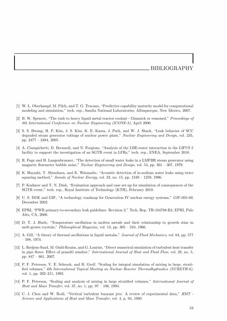
BIBLIOGRAPHY
[1] W. L. Oberkampf, M. Pilch, and T. G. Trucano, “Predictive capability maturity model for computationalmodeling and simulation,” tech. rep., Sandia National Laboratories, Albuquerque, New Mexico, 2007.
[2] B. W. Spencer, “The rush to heavy liquid metal reactor coolant - Gimmick or reasoned,” Proceedings of8th International Conference on Nuclear Engineering (ICONE-8), April 2000.
[3] S. S. Hwang, H. P. Kim, J. S. Kim, K. E. Kasza, J. Park, and W. J. Shack, “Leak behavior of SCCdegraded steam generator tubings of nuclear power plant,” Nuclear Engineering and Design, vol. 235,pp. 2477 – 2484, 2005.
[4] A. Ciampichetti, D. Bernardi, and N. Forgione, “Analysis of the LBE-water interaction in the LIFUS 5facility to support the investigation of an SGTR event in LFRs,” tech. rep., ENEA, September 2010.
[5] R. Fuge and H. Langenbrunner, “The detection of small water leaks in a LMFBR steam generator usingmagnetic flowmeter bubble noise,” Nuclear Engineering and Design, vol. 54, pp. 301 – 307, 1979.
[6] K. Hayashi, Y. Shinohara, and K. Watanabe, “Acoustic detection of in-sodium water leaks using twicesquaring method,” Annals of Nuclear Energy, vol. 23, no. 15, pp. 1249 – 1259, 1996.
[7] P. Kudinov and T. N. Dinh, “Evaluation approach and case set-up for simulation of consequences of theSGTR event,” tech. rep., Royal Institute of Technology (KTH), February 2010.
[8] U. S. DOE and GIF, “A technology roadmap for Generation IV nuclear energy systems,” GIF-002-00,December 2002.
[9] EPRI, “PWR primary-to-secondary leak guidelines Revision 2,” Tech. Rep. TR-104788-R2, EPRI, PaloAlto, CA, 2000.
[10] D. T. J. Hurle, “Temperature oscillation in molten metals and their relationship to growth stiae inmelt-grown crystals,” Philosophical Magazine, vol. 13, pp. 305 – 310, 1966.
[11] A. Gill, “A theory of thermal oscillations in liquid metalss,” Journal of Fluid Mechanics, vol. 64, pp. 577– 588, 1974.
[12] L. Redjem-Saad, M. Ould-Rouiss, and G. Lauriat, “Direct numerical simulation of turbulent heat transferin pipe flows: Effect of prandtl number,” International Journal of Heat and Fluid Flow, vol. 28, no. 5,pp. 847 – 861, 2007.
[13] P. F. Peterson, V. E. Schrock, and R. Greif, “Scaling for integral simulation of mixing in large, strati-fied volumes,” 6th International Topical Meeting on Nuclear Reactor Thermalhydraulics (NURETH-6),vol. 1, pp. 202–211, 1993.
[14] P. F. Peterson, “Scaling and analysis of mixing in large stratified volumes,” International Journal ofHeat and Mass Transfer, vol. 37, no. 1, pp. 97 – 106, 1994.
[15] C. J. Chen and W. Rodi, “Vertical turbulent buoyant jets: A review of experimental data,” HMT -Science and Applications of Heat and Mass Transfer, vol. 4, p. 94, 1980.
53

54 Bibliography
[16] E. J. List, “Turbulent jets and plumes,” Annual Review of Fluid Mechanics, vol. 14, pp. 189 – 212, 1982.
[17] F. Cadinu, M. Jeltsov, W. Villanueva, K. Koop, A. Karbojian, and P. Kudinov, “Program of work forexperimental tasks, software development and validation tasks on TALL,” tech. rep., Royal Institute ofTechnology (KTH), 2011.
[18] F. C. M. Jeltsov, W. Villanueva, K. Koop, A. Karbojian, and P. Kudinov, “An approach to validationof coupled CFD and System Thermal-Tydraulics codes,” 14th International Topical Meeting on NuclearReactor Thermalhydraulics (NURETH-14), 2011.
[19] W. Ma, E. Bubelis, A. Karbojian, B. R. Sehgal, and P. Coddington, “Transient experiments from thethermal-hydraulic ADS lead bismuth loop (TALL) and comparative TRAC/AAA analysis,” NuclearEngineering and Design, vol. 236, 2006.
[20] Star-CCM+ User Guide version 5.06.
[21] W. Xu, Q. Chen, and F. T. M. Nieuwstadt, “A new turbulence model for near-wall natural convection,”International Journal of Heat and Mass Transfer, vol. 41, 1998.
[22] W. L. Oberkampf, S. M. DeLand, B. M. Rutherford, K. V. Diegert, and K. F. Alvin, “Error anduncertainty in modeling and simulation,” Reliability Engineering & System Safety, vol. 75, no. 3, pp. 333– 357, 2002.
[23] T. G. Theofanus, “On the proper formulation of safety goals and assessment of safety margins for rareand high-consequence hazards,” Reliability Engineering and System Safety, vol. 54, pp. 243 – 257, 1996.
[24] M. Pourgol-Mohamad, A. Mosleh, and M. Modarres, “Structured treatment of model uncertainty incomplex thermal-hydraulics codes: Technical challenges, prospective and characterization,” NuclearEngineering and Design, vol. 241, pp. 285 –295, 2011.
[25] I. Leibson, E. G. Holcomb, A. G. Cacoso, and J. J. Jacmic, “Rate of flow and mechanics of bubbleformation from single submerged orifices,” AIChE Journal, vol. 2, p. 296, 1956.
[26] A. Marmur and E. Rubin, “Equilibrium shapes and quasi-static formation of bubbles at submergedorifice,” Chemical engineering Science, vol. 28, p. 1455, 1973.
[27] A. A. Kulkarni and J. B. Joshi, “Bubble formation and bubble rise velocity in gas-liquid systems: Areview,” Industrial & Engineering Chemistry Research, vol. 44, no. 16, pp. 5873–5931, 2005.
[28] K. Terasaka, Y. Sasada, D. Kobayashi, and S. Fujioka, “Submilli-bubble dispersion from a slit orificeinto water,” Journal of Chemical Engineering, vol. 44, no. 3, pp. 140 – 145, 2011.
[29] A. V. Beznosov, S. S. Pinaev, D. V. Davydov, A. A. Molodtsov, T. A. Bokova, P. N. Martynov, and V. I.Rachkov, “Experimental studies of the characteristics of contact heat exchange between lead coolantand the working body,” Atomic Energy, vol. 98, no. 3, 2005.
[30] B. Flesch and B. Cochet, “Leak-Before-Break in steam generator tubes,” International Journal of Pres-sure Vessels and Piping, vol. 43, pp. 165 – 179, 1990.
[31] S. S. Hwang, H. P. Kim, and J. S. Kim, “Evaluation of the burst characteristics for axial notches on SGtubings,” Nuclear Engineering and Design, vol. 232, pp. 139 – 143, 2004.
[32] S. S. Hwang, C. Namgung, M. K. Jung, H. P. Kim, and J. Kim, “Rupture pressure of wear degradedalloy 600 steam generators tubings,” Journal of Nuclear Materials, vol. 373, pp. 71 – 74, 2008.
[33] G. Yang, B. Du, and L. Fan, “Bubble formation and dynamics in gas-liquid-solid fluidization - A review,”Chemical Engineering Science, vol. 62, no. 1-2, pp. 2 – 27, 2007. Fluidized Bed Applications.
[34] R. Clift, J. R. Grace, and M. E. Weber, Bubbles, drops and particles. Academic Press, Inc., 1978.
[35] C. C. Maneri and P. F. Vassallo, “Dynamics of bubbles rising in finite and infinite media,” Tech. Rep.LM-00K048, Lockheed Martin Corporation, Schenectady, NY 12301 (US), 2000.
[36] OECD and NEA, “Handbook on lead-bismuth eutectic alloy and lead properties, materials compatibility,thermal-hydraulics and technologies,” 2007.
[37] CD-Adapco, Star-CCM+ User Guide version 5.02.

Bibliography 55
[38] D. G. Karamanev and L. N. Nikolov, “Free rising bubbles do not obey Newton’s law for free settling,”AIChE Journal, vol. 38, pp. 1993 – 1997, 1992.
[39] S. L. Sullivan and B. W. Hardy, “Formation of air bubbles at orifices submerged below liquid,” AIChEJournal, vol. 10, p. 848, 1964.
[40] D. Rodrigue, “A simple correlation for gas bubbles rising in power-law fluids,” Canadian Journal ofChemical Engineering, vol. 80, no. 2, p. 289, 2002.
[41] A. Tomiyama, I. Kataoka, I. Zun, and T. Sakaguchi, “Drag coefficients of single bubbles under normaland microgravity conditions,” JSME International Journal Series D, vol. 41, no. 2, p. 472, 1998.
[42] H. D. Mendelson, “The prediction of bubble terminal velocities from wave theory,” AIChE Journal,vol. 13, p. 250, 1967.
[43] Y. Mori, K. Hijikata, and K. Kuriyama, “Experimental study of bubble motion in mercury with andwithout a magnetic field,” Journal of Heat Transfer (Trans. ASME), vol. 99, pp. 404–410, 1977.
[44] A. Alemberti, J. Carlsson, E. Malambu, A. Orden, L. Cinotti, D. Struwe, P. Agostini, and S. Monti,“ELSY – European LFR activities,” Journal of Nuclear Science and Technology, vol. 48, no. 4, pp. 479– 482, 2011.
[45] L. Cinotti, “Reactor assembly preliminary configuration,” Tech. Rep. ELSY DOC 08 049, Del FungoGiera Energia S.p.A., 2008.
[46] M. Bottcher, “CFD analysis of decay heat removal scenarios of the lead cooled ELSY reactor,” Bench-marking of CFD Codes for Application to Nuclear Reactor Safety (CFD4NRS-3), September 14-16 2010.
[47] A. Onea, M. Bottcher, and D. Struwe, “Lead pressure loss in the heat exchanger of the ELSY fast lead-cooled reactor by CFD approach,” Benchmarking of CFD Codes for Application to Nuclear ReactorSafety (CFD4NRS-3), September 14-16 2010.
[48] J. Carlsson, “Steam generator tube leakage calculations on the ELSY design,” tech. rep., EC JRC,Institute for Energy, 2009.