International Journal of Current Engineering and Technology E-ISSN 2277 – 4106, P-ISSN 2347 – 5161 ©2016 INPRESSCO®, All Rights Reserved Available at http://inpressco.com/category/ijcet

Research Article

192| MIT College of Engineering, Pune, India, AMET 2016, INPRESSCO IJCET Special Issue-4 (March 2016)

CFD Analysis of Centrifugal Pump’s Impeller of Various Designs and Comparison of Numerical Results for Various Models Rajiv Kaul* College of Military Engg. Pune-31, India Accepted 03 March 2016, Available online 15 March 2016, Special Issue-4 (March 2016)

Abstract The flow through the impeller of a Centrifugal pump is complicated and tedious. Computational Fluid Dynamics (CFD) simulation of a pump provides a complete picture of its operation, and allows identifying most profound design parameters. Many technical applications of Centrifugal pumps cannot be fulfilled without proper analysis, especially regarding pumps parameters i.e. blades angle, material, head, discharge and number of blades. Pressure pulsations may be troublesome during the operation and performance of Centrifugal pumps. The output from the CFD analyses provides a time history of the pressure variation and performance characteristics as the impeller rotates in the volute for various impellers design (blades angles). This paper deals with the design and numerical analysis of Centrifugal pump. A design of Centrifugal pump is carried out and numerically analyzed to get the best performance point. The Centrifugal pumps impellers under consideration were designed and modeled as a “radial” type (6-blades, semi-shrouded) with blades angles (150, 280; 180,300) in which the flow noise or pulsation generally remains low. Keywords: Impeller, blade angles, Ansys, Introduction

1 Turbulent Flow is characterized by random and rapid fluctuations swirling regions of fluid (eddies) throughout the flow. These fluctuations provide an additional mechanism for momentum and energy transfer. The swirling eddies transport mass, momentum and energy to other regions of flow much more rapidly than molecular diffusion, greatly enhancing mass, momentum and heat transfer. As a result, turbulent flow is associated with much higher values of friction, heat transfer and mass transfer coefficients. Even when the average flow is steady, the eddy motion in turbulent flow causes significant fluctuations in the values of velocity, temperature, pressure and even density. Turbulence brings fluids of different momentum contents into contact. The reduction of the velocity gradient produced by the action of viscosity reduced the kinetic energy of the flow, so that the action is dissipative. In fully developed turbulent flow, the flow quantities are random quantities. It implies that in turbulent flow, the velocity flow field varies significantly and irregularly in both position and time. The flow may be considered to be the super- position of a main flow with irregular fluctuation in the velocity or in other fluids mechanical quantities. The velocity field is therefore represented as follows:

( ) ( ) ( ) (1)

*Corresponding author: Rajiv Kaul

This decomposition is particularly appropriate if the fluctuation velocity ui’ is much smaller than mean velocity . The magnitude of ui’ is just a few percent of but high frequencies of eddies makes them very effective for the transport of momentum, thermal energy and mass. Navier-Stokes equation for turbulent flow in 3D, for incompressible fluid

+

(2)

+

(3)

+

(4)

Where X,Y,Z are components of body forces in x-, y- and z-direction, respectively; whereas- , and p represent fluid density, dynamic viscosity and acting pressure, respectively. These equations are very much similar to the equations which are used for laminar flow except the viscous terms augmented by the Reynolds stresses. In order to determine the Reynolds stress term it becomes necessary to resort to assumptions about its behavior in turbulent flow. These assumptions are based partly on theoretical analysis and partly on experimental results, and are collectively known as

Rajiv Kaul CFD Analysis of Centrifugal Pump’s Impeller

193| MIT College of Engineering, Pune, India, AMET 2016, INPRESSCO IJCET Special Issue-4 (March 2016)

turbulence modeling. In all, aim is to express Reynolds stress as a function of the mean flow.

Turbulence Models

Turbulent flows are commonly encountered in practical applications. It is the time-mean behavior of the flows that is usually of practical interest. Therefore, the equations for unsteady laminar flow are converted into the time-averaged equations for turbulent flow by an averaging operation in which it is assumed that there are rapid and random fluctuations about the mean value. The additional terms arising from this operation are the Reynolds stresses, turbulent diffusion flux etc. To express these fluxes in terms of the mean properties of the flow is the task of turbulence model. Many turbulence models employ the concept of a turbulent viscosity or a turbulent diffusivity to express the turbulent stresses and fluxes. The result is that the time –averaged equations for the turbulent flow have the same appearance as the equations for the laminar flow, but the laminar exchange coefficients such as viscosity, diffusivity and conductivity are replaced by effective (laminar plus turbulent) exchange coefficients.

Turbulence Models Two Equation Models (Average Reynolds No N-S equation (RANS) based) :- (a) Standard k- (b) RNG k- (c) Realizable k- (d) Standard k- (e) Shear Stress Transport Model (SST) (f) Reynolds stress Model (g) SST Transition Model :- Standard k- Model: In this model, robust low –Reynolds number formulation down to the viscous sub-layer exists. It also takes care of compressibility effects, transitional flows and shear flow corrections and adverse pressure gradient. This model is very much sensitive to free-stream gradient. It is most widely adopted in the aerospace and turbo-machinery.

k- Model uses the turbulence frequency ( =/k) as

the second variable and length scale, ƪ=√ . Hence

eddy viscosity is given by .

Shear Stress Transport Model (SST Model) : It is the variation of the standard k-ε model. It is so named because the definition of turbulent viscosity is modified to account for the transport of the principal turbulent shear stress. It takes into account the transport of turbulent shear stress, and makes a gradual change of solution variables from the standard k-ε model in the inner region of the boundary layer to a high Reynolds number version in the outer part of the boundary layer. 1. The results of the k- are much less sensitive to the (arbitrary) assumed values in the free stream, but its near wall performance is unsatisfactory for boundary layers with adverse pressure gradients. This

led to use (i) a transformation of the k- model into a k- model in the near –wall region (ii) the standard k- model in the fully turbulence. CFD Design Considerations

Solid modeling is at the core of this integrated design and analysis system. The solid model also provides the grid for finite volume (FV) simulation. Geometry generation starts with curve manipulation, such as hub/shroud curve, blade angle, or thickness profiles. Most parameters are defined though interactively editable curves (for shaping blades). These curves have the distinct advantage of being continuous in each derivative and require a minimal number of points to define viable shape. A laboratory pump that can suit radial impellers with the same diameter (134 mm) has been designed and modeled. Initially, semi shrouded impellers with outlet blade angle 280 and 300 respectively, were designed and with the aid of computational flow dynamics, the flow patterns through the pump as well as its performance in design and off-design operation were analyzed/predicted. The pump is divided into three regions:- inlet, rotary, casing with outlet. First 3D modeling has been done using dimension of pumps impeller. Then inlet, impeller, casing and outlet region was meshed using tetra-hedral elements independently; structured grids are used for inlet and casing, but a mixture of structured and unstructured grids are used for the rotary regions and outlet region. Then using turbulence models (k-ω and SST) and inputs (inlet velocity and pressure, rotating speed of impeller, discharge), results were analyzed. In technically relevant fluid pressure, the flow occurs relative to stationary walls or moving structure (such as impeller). Although the fluid near the wall comprises only a fraction of the flow field, it largely determines losses and velocity distribution in or around a component. It is assumed that the relative motion is zero immediate at the wall (no-slip condition) and that no gradients of static pressure occurs perpendicular to the

wall within the boundary layer (

).

Consequently, the core flow imparts the pressure to the boundary layer and determines the pressure distribution in the flow field under consideration. All

streamlines have the same pressure gradient (

) in

the flow direction but posses different amount of kinetic energy. Owing to the no-slip condition, the fluid adhering to a stationary wall has absolute velocity of zero. In contrast, on the walls of a rotating impeller it has a relative velocity of zero. Accordingly, a fluid particle adhering to the blades of an impeller moves with the absolute velocity (u=ω.r). The transition from a laminar to a turbulent boundary layer depends on:- Reynolds Number, surface roughness, turbulence of the outer flow, pressure gradient, and wall curvature.

Rajiv Kaul CFD Analysis of Centrifugal Pump’s Impeller

194| MIT College of Engineering, Pune, India, AMET 2016, INPRESSCO IJCET Special Issue-4 (March 2016)

Table 1: Denomination of Impeller (type A)

Denomination Value (type A) Impeller blades angles β1 = 15°, β2 =280 Suction pipe diameter,

Ds =50mm ,

Number of blades, Head z = 6, 8—13 m

Impeller diameters ( Al)

D1 = 58mm, D2 = 134mm

Flow rate in best efficiency point,

Q = 0.55 -4 lit/s, N = 2500 to 3200rpm, vel—1.72—3.2m/s

Impeller blades widths, height

b1= 2m, b2= 4.2mm, h=8-9mm

Number of blades, Head z = 6, 10 -15 m

Table 2: Denomination of New Impeller (type B)

Denomination Value (type B) Impeller blades angles β1 = 18 °, β2 =30°

Suction pipe diameter Ds =50mm Number of blades, Head z = 6, 8—13 m

Impeller diameters (Al) D1 = 58mm, D2 = 134mm

Flow rate in best efficiency point,

Q = 0.5 — 4.5 lit/s, N =2200 — 3200 rpm, vel—1.5—3.78 m/s

Impeller blades width, height

b1=2mm, b2= 4 mm, h=8-9mm

Specific speed Ns = 650-1000

Fig.1: Boundary layer transition from laminar to

turbulent

In the present investigations, numerical analysis of

the various impellers design (β1 = 15°, β2 =280; β1 =

18 °, β2 =30°) were carried out assuming various

turbulent models (k-ω and SST). To make impeller

lighter and of high degree of surface finishing,

Aluminium has been selected while other parts are

made of CI.

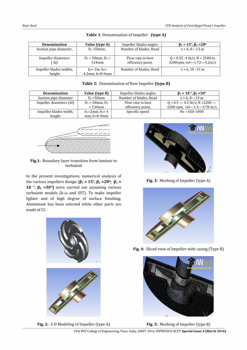
Fig. 2: 3-D Modeling of Impeller (type A)

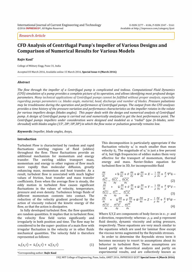
Fig. 3: Meshing of Impeller (type A)

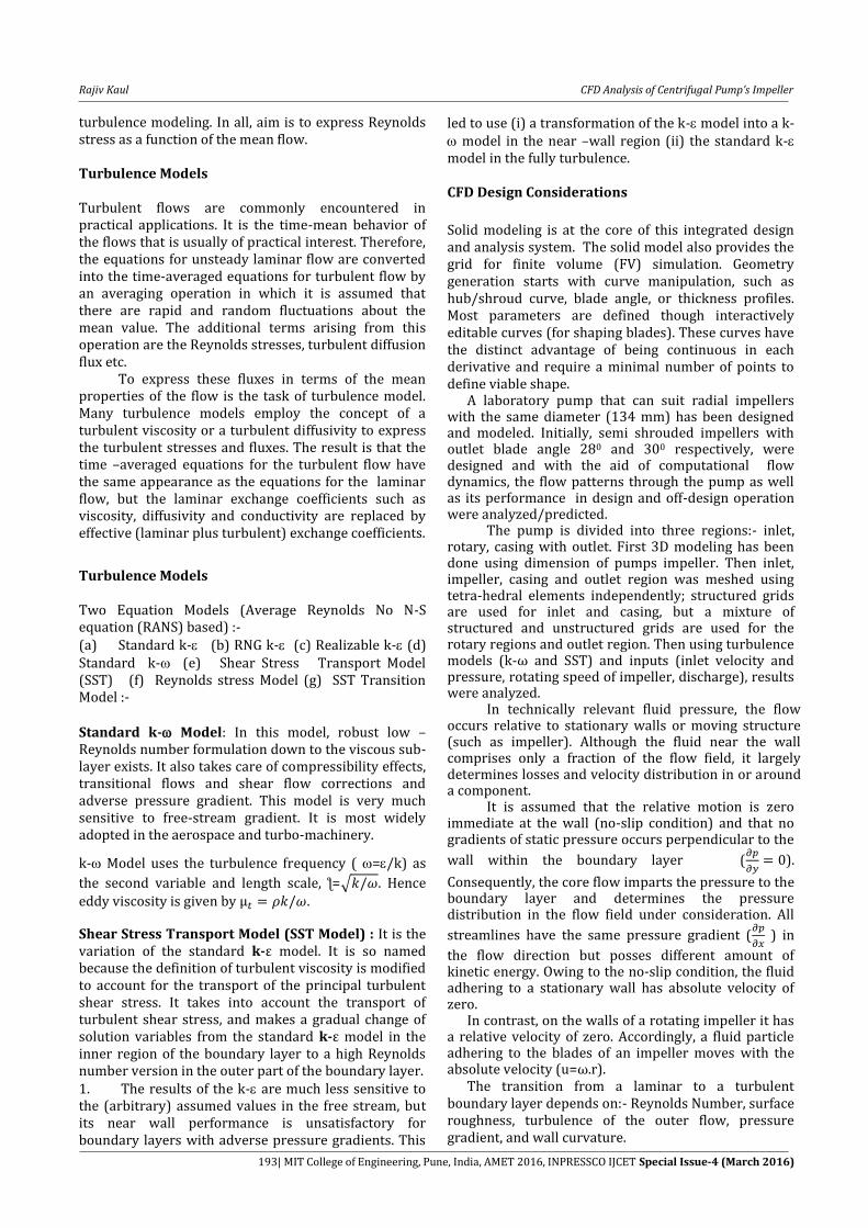
Fig. 4: Sliced view of Impeller with casing (Type B)

Fig. 5: Meshing of Impeller (type B)

Rajiv Kaul CFD Analysis of Centrifugal Pump’s Impeller

195| MIT College of Engineering, Pune, India, AMET 2016, INPRESSCO IJCET Special Issue-4 (March 2016)

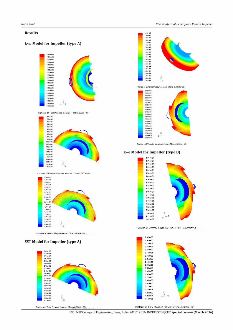
Results

k-ω Model for Impeller (type A)

SST Model for Impeller (type A)

k-ω Model for Impeller (type B)

Rajiv Kaul CFD Analysis of Centrifugal Pump’s Impeller

196| MIT College of Engineering, Pune, India, AMET 2016, INPRESSCO IJCET Special Issue-4 (March 2016)

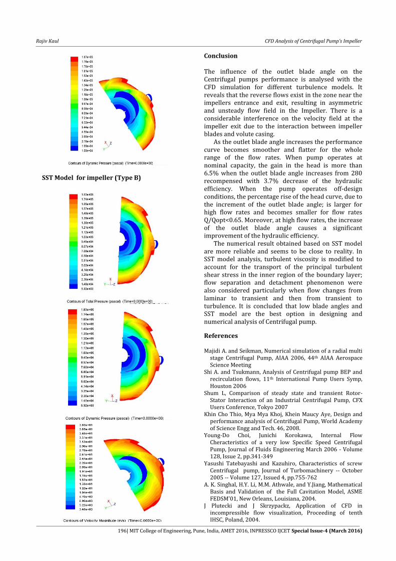
SST Model for impeller (Type B)

Conclusion

The influence of the outlet blade angle on the Centrifugal pumps performance is analysed with the CFD simulation for different turbulence models. It reveals that the reverse flows exist in the zone near the impellers entrance and exit, resulting in asymmetric and unsteady flow field in the Impeller. There is a considerable interference on the velocity field at the impeller exit due to the interaction between impeller blades and volute casing. As the outlet blade angle increases the performance curve becomes smoother and flatter for the whole range of the flow rates. When pump operates at nominal capacity, the gain in the head is more than 6.5% when the outlet blade angle increases from 280 recompensed with 3.7% decrease of the hydraulic efficiency. When the pump operates off-design conditions, the percentage rise of the head curve, due to the increment of the outlet blade angle; is larger for high flow rates and becomes smaller for flow rates Q/Qopt<0.65. Moreover, at high flow rates, the increase of the outlet blade angle causes a significant improvement of the hydraulic efficiency. The numerical result obtained based on SST model are more reliable and seems to be close to reality. In SST model analysis, turbulent viscosity is modified to account for the transport of the principal turbulent shear stress in the inner region of the boundary layer; flow separation and detachment phenomenon were also considered particularly when flow changes from laminar to transient and then from transient to turbulence. It is concluded that low blade angles and SST model are the best option in designing and numerical analysis of Centrifugal pump.

References Majidi A. and Seikman, Numerical simulation of a radial multi

stage Centrifugal Pump, AIAA 2006, 44th AIAA Aerospace Science Meeting

Shi A. and Tsukmann, Analysis of Centrifugal pump BEP and recirculation flows, 11th International Pump Users Symp, Houston 2006

Shum L, Comparison of steady state and transient Rotor-Stator Interaction of an Industrial Centrifugal Pump, CFX Users Conference, Tokyo 2007

Khin Cho Thio, Mya Mya Khoj, Khein Maucy Aye, Design and performance analysis of Centrifugal Pump, World Academy of Science Engg and Tech. 46, 2008.

Young-Do Choi, Junichi Korokawa, Internal Flow Cheracteristics of a very low Specific Speed Centrifugal Pump, Journal of Fluids Engineering March 2006 - Volume 128, Issue 2, pp.341-349

Yasushi Tatebayashi and Kazuhiro, Characteristics of screw Centrifugal pump, Journal of Turbomachinery -- October 2005 -- Volume 127, Issued 4, pp.755-762

A. K. Singhal, H.Y. Li, M.M. Athwale, and Y.Jiang, Mathematical Basis and Validation of the Full Cavitation Model, ASME FEDSM'01, New Orleans, Louisiana, 2004.

J Plutecki and J Skrzypackz, Application of CFD in incompressible flow visualization, Proceeding of tenth IHSC, Poland, 2004.