CERTAIN SYSTEMS ARISING IN STOCHASTIC GRADIENT …
103
CERTAIN SYSTEMS ARISING IN STOCHASTIC GRADIENT DESCENT Konstantinos Karatapanis A DISSERTATION in Mathematics Presented to the Faculties of the University of Pennsylvania in Partial Fulfillment of the Requirements for the Degree of Doctor of Philosophy 2019 Supervisor of Dissertation Robin Pemantle, Professor of Mathematics Acting Graduate Group Chairperson David Harbater, Professor of Mathematics Dissertation Committee: Robin Pemantle, Professor of Mathematics Philip Gressman, Professor of Mathematics Henry Towsner, Associate Professor of Mathematics
Transcript of CERTAIN SYSTEMS ARISING IN STOCHASTIC GRADIENT …

CERTAIN SYSTEMS ARISING IN STOCHASTIC GRADIENTDESCENT
Konstantinos Karatapanis
A DISSERTATION
in
Mathematics
Presented to the Faculties of the University of Pennsylvania in PartialFulfillment of the Requirements for the Degree of Doctor of Philosophy
2019
Supervisor of Dissertation
Robin Pemantle, Professor of Mathematics
Acting Graduate Group Chairperson
David Harbater, Professor of Mathematics
Dissertation Committee:Robin Pemantle, Professor of MathematicsPhilip Gressman, Professor of MathematicsHenry Towsner, Associate Professor of Mathematics

Acknowledgments
I would like to thank my advisor Robin Pemantle for his continuous support,
throughout my years at Penn. He was a teacher to me not only in math with
his knowledge but also in life with him kind character.
Also I wish to thank my friends at Penn for supporting me. Among them I wish
to especially thank Albert Chenchao, and Giorgos Gounaris for the stimulating
conversations about my research.
Lastly, I owe a big thanks to my family for always being there for me, and a
special thanks to my grandmother.
ii

ABSTRACT
CERTAIN SYSTEMS ARISING IN STOCHASTIC GRADIENT DESCENT
Konstantinos Karatapanis
Robin Pemantle
Stochastic approximations is a rich branch of probability theory and has a wide
range of application. Here we study stochastic approximations from the perspective
of gradient descent. An important question is what is the asymptotic limit of a
stochastic approximation. In that spirit we will provide a detailed description for
the limiting behavior of certain one dimensional stochastic approximations.
iii

Contents
1 Introduction 1
1.1 Introduction . . . . . . . . . . . . . . . . . . . . . . . . . . . . . . . 1
1.2 Step sizes . . . . . . . . . . . . . . . . . . . . . . . . . . . . . . . . 4
1.3 Stochastic gradient descent . . . . . . . . . . . . . . . . . . . . . . . 7
1.4 Stochastic approximations . . . . . . . . . . . . . . . . . . . . . . . 9
1.4.1 Historic development . . . . . . . . . . . . . . . . . . . . . . 9
1.4.2 Convergence in one dimension . . . . . . . . . . . . . . . . . 12
1.4.3 Convergence in multiple dimensions . . . . . . . . . . . . . . 14
1.4.4 Motivating example . . . . . . . . . . . . . . . . . . . . . . . 18
1.5 Non-convex optimization . . . . . . . . . . . . . . . . . . . . . . . . 19
1.6 Further discussion . . . . . . . . . . . . . . . . . . . . . . . . . . . . 22
1.7 Results for the continuous model . . . . . . . . . . . . . . . . . . . 23
1.8 Results for the discrete model . . . . . . . . . . . . . . . . . . . . . 26
1.9 Further conjectures . . . . . . . . . . . . . . . . . . . . . . . . . . . 32
iv
2 Preliminary results 37
3 Continuous model 41
3.1 Continuous model, simplest case . . . . . . . . . . . . . . . . . . . . 41
3.1.1 Introduction . . . . . . . . . . . . . . . . . . . . . . . . . . . 41
3.1.2 Analysis of Xt when k ≥ 1/2. . . . . . . . . . . . . . . . . . 43
3.1.3 Analysis of Xt when k < 1/2. . . . . . . . . . . . . . . . . . 48
3.2 Analysis of dLt = |Lt|ktγ
dt+ 1tγ
dBt. . . . . . . . . . . . . . . . . . . . 52
3.2.1 Introduction . . . . . . . . . . . . . . . . . . . . . . . . . . . 52
3.2.2 Analysis of Xt when 1/2 + 1/2k ≥ γ, k > 1 and γ ∈ (1/2, 1) 56
3.2.3 Analysis of Xt when 12
+ 12k< γ, and k > 1 . . . . . . . . . 60
3.3 Analysis of dLt = f(Lt)tγ
dt+ 1tγ
dBt . . . . . . . . . . . . . . . . . . 66
4 The discrete model 69
4.1 Analysis of Xn when 12
+ 12k> γ, k > 1 and γ ∈ (1/2, 1) . . . . . . 69
4.2 Analysis of Xn when 12
+ 12k< γ, k > 1 and γ ∈ (1/2, 1) . . . . . . 77
4.3 Analysis of Xt when k > 1/2 and γ = 1 . . . . . . . . . . . . . . . . 82
4.4 Analysis of Xn when k < 1/2 and γ = 1 . . . . . . . . . . . . . . . 86
v

Chapter 1
Introduction
1.1 Introduction
Let F : Rd → Rd, d ≥ 1 be a vector field. For much of what follows, F arises as
the gradient of a potential function V , namely V : Rd → R, and F = −∇V . Now,
we define a system driven by
Xn+1 = Xn + an (F (Xn) + ξn+1) . (1.1.1)
To elaborate on the parameters, let Fn be a filtration, then an, ξn are adapted,
and ξn constitute martingale differences, i.e., E(ξn+1|Fn) = 0. The sequence an
can be deterministic or stochastic, and the sequence is assumed to be positive al-
most surely and is either converging to zero or staying constant, for a discussion
on the different possibilities, see section 1.2. Also, when the dynamics of F are
1

complicated, we usually require some additional assumptions on the the noise; one
is a boundedness restraint in that we assume the existence of a constant M , such
that |ξn| ≤M a.s.; and secondly, we want ξn to be quasi-isotropic (see [DKLH18]),
i.e., P((θ · ξn)+ > δ) > δ for any unit direction θ ∈ Rd . This condition makes
sure that the process gets jiggled in every direction. However, in many instances
more relaxed conditions on ξn are enough. This versatile system is well-studied,
and it arises naturally in many different areas. In machine learning and statistics,
(1.1.1) can be a powerful tool used for quick optimization and statistical inference
(see [AAZB+17], [LLKC18], [CdlTTZ16]), among other uses. Furthermore, many
urn models are represented by (1.1.1). These processes play a central role in prob-
ability theory due to their wide applicability in physics, biology and social sciences;
for a comprehensive exposition on the subject see [Pem07].
Processes satisfying (1.1.1), when an goes to zero, are known as stochastic ap-
proximations, first introduced in [RM51]. These processes have been extensively
studied since [KY03]. An important feature is that the step size an satisfies
∑n≥1
an =∞ and∑n≥1
a2n <∞.
This property balances the effects of the noise in the system, so that there is an
implicit averaging that eventually, eliminates the effects of the noise. The pre-
viously described system hence behaves similarly to the mean flow: the ODE
whose right-hand side corresponds to the expectation of the driving term (F (Xt)).
2

The previous heuristic can help us identify the support S of the limiting process
X∞ := limn→∞Xn in terms of the topological properties of the dynamical system
dXtdt
= F (Xt) (see [KY03] chapter 5). More specifically, in most instances, one can
argue that attractors are in S, whereas repellers or “strict” saddle points are not
(see [KY03] chapter 5.8). However, there has not been a systematic approach find-
ing when a degenerate saddle point, i.e., a point that is neither an attractor nor a
repeller, belongs in S.
Stochastic approximations arise naturally in many different contexts. Some
early results were published by [Rup88] and [PJ92]. There, they dealt with averaged
stochastic gradient descent (ASGD) arising from a strongly convex potential V with
step size n−γ, γ ∈ (1/2, 1]. In their work they proved that one can build, with proper
scaling, consistent estimators xn (for the arg min(V )) whose limiting distribution
is Gaussian. In learning problems, a modified version of ASGD [RSS12] provides
convergence rates to global minima of order n−1. Additionally, many classical urn
processes can be described via (1.1.1), where an is of the order of n−1. Focused
effort is being placed in understanding the support of the limiting process X∞. In
specific instances, the underlying problem boils down to understanding an SGD
problem: characterizing the support of X∞ in terms of the set of critical points of
the corresponding potential V . For a comprehensive exposition on urn processes,
see [Pem07].
3

1.2 Step sizes
In the literature of stochastic approximations, there is are ample choices for the
behavior of the step sizes depending on the application at hand. Also, in different
contexts, the sequence an as in recursion (1.1.1) can appear with different names.
For example it is known as learning rate (machine learning), smoothing constant
(forecasting) or gain (signal processing).
1. In [EDM04] they study the rate of convergence for polynomial step sizes, i.e.,
an = n−γ where γ ∈ (1/2, 1) in the context of Q-learning for Markov decision
processes, and they experimentally demonstrate that for γ, approximately 1720
the rate of convergence is optimal.
2. Kesten algorithm [Kes58] introduced a stochastic approximation process in
hopes of accelerating the convergence of the Robbins-Monro algorithm [RM51].
The idea here is: when we are confident that the process is close to the value
θ we wish to estimate, we decrease the step size in order to stabilize the con-
vergence. And whenever we suspect we are far away from θ, we keep the step
size large in order to allow faster exploration. In order to determine when it
is warranted to decrease the step size, they followed the heuristic that when
the process is close to θ then the sign of Xn − Xn−1 should fluctuate more
intensely, as the process will keep overshooting. More formally, suppose that
we have a sequence an ≥ 0 such that∑
n=1 an =∞ and∑
n=1 a2n <∞. Then
4

we define a stochastic approximation whose step size is b1 = a1, b2 = a2 and
bn = akn
kn+1 =
kn if (Xn −Xn−1)(Xn−1 −Xn−2) > 0
kn + 1 if (Xn −Xn−1)(Xn−1 −Xn−2) ≤ 0
3. In Gaivoronski [EW88], we see another variation of the Robbins-Monro al-
gorithm where the step size is decreasing when |Xn−Xn−k|∑n−1i=n−k |Xi+1−Xi|
≤ γ for some
threshold value γ, and otherwise it stays the same. The intuition on why this
works is that the quantity |Xn−Xn−k|∑n−1i=n−k |Xi+1−Xi|
≤ γ is small when the iterates are
fluctuating, and this is likely to happen when you are in the proximity of the
minimum. Conversely, when the quantity |Xn−Xn−k|∑n−1i=n−k |Xi+1−Xi|
is big, the process
is likely to be far away from the minimum.
4. In [SR96], they study the adaptive behavior of a lizard. In this model, the
lizard wants to maximize the reward per unit of time in the long run. The
lizard is at its home, unless it is hunting, and at some random time τn an ant
appears whose weight is wn. If the lizard is at home and an ant appears, it
decides whether to go after the ant or not. If the lizard goes after the ant, it
will catch it with some probability and it will take the lizard rn to return to
its home, regardless of whether he has successfully captured its prey or not.
More formally, the lizard decides, based on past observations, to chase after
the ant having in mind to maximize Tn/Wn the ratio of the total time it has
5

taken him to successfully have caught ants whose total weight amounts to Wn.
This problem can be formulated as a stochastic approximation, whose step
size is W−1n . The purpose of this research is to compare whether the strategy
utilized by the lizard in this learning problem, will match the strategy that
would arise via different optimization techniques; for example via the “return
for effort” principle.
5. In [PJ92] and [Rup19] the step sizes are of polynomial order an = n−γ. Here,
they focus on studying an average of the iterates Sn =∑ni=1Xian
properly scaled
so that Sn converges in distribution to a normal. The optimal choice for γ is
shown be less than 1, indicating that if you allow more fluctuations then by
averaging you obtain a better estimate for the true value of the parameter.
The point estimation for Robbins-Monro can be shown to be optimal for step
size an = 1n
in terms of minimizing the square mean error at comparable rates
to the averaging scheme. Even though we do not improve the performance
in the long run, the averaging scheme is preferable since the larger step sizes
increase robustness because in the early stages it is favorable to increase the
rate of exploration.
6
1.3 Stochastic gradient descent
In machine learning, processes satisfying (1.1.1) appear in stochastic gradient de-
scent (SGD). First, to provide context, let us briefly introduce the gradient descent
method (GD) and then see why SGD arises naturally from it. The GD is an op-
timization technique which finds local minima for a potential function V via the
iteration
xn+1 − xn = −ηn∇V (xn), (1.3.1)
where in many applications we take ηn to be a positive and constant. Notice that
(1.3.1) is a specialization of (1.1.1), when F = −∇V , ξn+1 ≡ 0 and an = ηn. The
previous method when applied to non-convex functions has the shortcoming that
it may get stuck near saddle points, i.e., points where the gradient vanishes, that
are neither local minima nor local maxima, or locate local minima instead of global
ones. The former issue can be resolved by adding noise into the system, which,
consequently, helps in pushing the particle downhill and eventually escaping saddle
points (see [Pem90] and [KY03] chapter 5.8). For the latter, in general, avoiding
local minima is a difficult problem ([GM91] and [RRT17]), however, fortunately,
in many instances finding local minima is satisfactory. Recently, there have been
several problems of interest where this is indeed the case, either because all local
minima are global minima ([GHJY15] and [SQW17]), or because in other cases local
minima provide equally good results as global minima [CHM+15]. Furthermore, in
7

certain applications saddle points lead to highly sub-optimal results ([JJKN15] and
[SL16]), which highlights the importance of escaping saddle points.
An important variant of GD/SGD is the momentum GD/SGD, firstly intro-
duced by Polyak in [Pol64]. This algorithm diminishes the effects of the gradient in
directions where the iterates are fluctuating, and it increases the movement along
stable directions by accumulating momentum. In the literature the momentum
algorithm appears in two popular formats,
vt = bvt−1 + η∇V (xt)
xt = xt−1 − vt−1
and
vt = bvt−1 + (1− β)∇V (xt)
xt = xt−1 − ηvt−1
The parameter β ∈ (0, 1), plays an important role in the performance. In practice,
usually β is chosen around 0.9, but there is no fast and hard rule. SGD has difficulty
navigating along ravines, and in such instances adding momentum can significantly
improve performance.
A small variation of the previous algorithm, but which significantly improves
performance is the accelerated gradient descent, or the look-ahead momentum gra-
8

dient descent [NES83].
vt = bvt−1 + η∇V (xt − bvt−1)
xt = xt−1 − vt−1
Here, in order to make the transition from xt−1 to xt, we incorporate into the
gradient the quantity −bvt−1 which is a good predictor on where the xt−1 will land,
hence further improving the performance and giving a convergence rate of O(1/t2)
after t iterations.
One shortcoming of the momentum algorithms already described is that we have
to guess the value of the parameter b as the these algorithms do not have a way to
auto-tune. Some variations of SGD that try to ameliorate this are Adagard [DHS11],
and Adadelta [DZ12]. For an overview for SGD algorithms with a neural network
perspective, see [Rud16].
1.4 Stochastic approximations
1.4.1 Historic development
In 1951, R. Monro gave birth to stochastic approximation with his work [RM51].
Time proved that his ideas were very fruitful, and since then the theory has flour-
ished. Suppose we perform an experiment at level xn ∈ [0, 1] giving rise to a random
9
variable ξ(ω, xn), whose distribution is unknown depending on xn, measuring the
response of the experiment. Here, E(ξ(ω, xn)) is again unknown, however we know
it is increasing in its second coordinate. We wish to find the level x such that
E(ξ(ω, x)) = a, where a is a given constant. This should be done by establishing
a recursive rule on how, given the past observations, we can determine the next
level xn+1 for the experiment so that xn → θ in some sense. This can be accom-
plished by the recursion xn+1 − xn = 1n(a − ξ(ω, xn)) . To make the connection to
(1.1.1), an = 1n, F (xn) = a−E(ξ(ω, xn)) and ξn+1 = E(ξ(ω, xn))−ξ(ω, xn). One of
the main theorems is that when E(ξ(ω, x)) is differentiable such that ∂E(ξ(ω,x))∂x
> 0
then xn → θ in probability. The step size factor 1n
is chosen appropriately, so that
there is an implicit averaging that eliminates the effects of the noise, eventually.
The previously described system hence behaves similarly to the ODE whose right-
hand side corresponds to the expectation of the driving term in the sense that their
limiting points coincide.
Later Kiefer [KW52], in a short paper, relaxed the conditions on M(x) =
E(ξ(ω, x)). In the following years Julius R. Blum first established that the con-
vergence in the R. Monro model is almost surely, and then later on he proved the
multidimensional analogue [RB54].
In an effort to improve the rate of convergence, in the multidimensional setting,
and make it more applicable in the field of statistics in [PJ92] they consider an
average of the iterates, i.e., Sn =∑n
i=1 xi. Then they show that if Sn is averaged
10

properly then, it converges in distribution to a normal random variable. In that
way it is possible to perform statistical testing like confidence intervals or hypothesis
testing. Next, we provide a motivating example:
Example 1. In paper [HLS80], they consider a random variable Xn taking values
in (0, 1), which we interpret as counting the percentage of the red balls out of n balls
in accordance to Polya’s urn model. Recursively define Xn+1 to benXn + 1
n+ 1with
probability f(Xn), and Xn+1 =nXn
n+ 1with probability 1 − f(Xn). The main result
of [HLS80] is that Xn converges to a random variable X, whose range is a subset
of C = p|f(p) = p; moreover for all points p such that f ′(p) < 1 or (f ′(p) > 1),
we have P(X = p) > 0 (P(X = p) = 0).
This process fits the general form (1.1.1). Indeed, we may rewrite Xn in the
following form Xn+1 −Xn = An + Yn where Yn is the martingale
Yn =
1−f(Xn)n+1
, with probability f(Xn)
, and An = f(Xn)−Xnn+1
.
−f(Xn)n+1
, with probability 1− f(Xn)
Define gn =
1− f(Xn), with probability f(Xn)
−f(Xn), with probability 1− f(Xn)
.
Then, the SDE becomes Xn+1 − Xn = f(Xn)−Xnn+1
+gn
n+ 1= f(Xn)−Xn
n+1+
Θ(1)
n+ 1,
when f(Xn) is bounded away from 0, 1. We have already mentioned that Xn can
only converge to points p, such that f(p) = p, f ′(p) < 1. The idea is that the
11

condition f ′(p) < 1 implies that f(Xn) − Xn is positive when Xn ∈ (p − δ, p) and
negative when Xn ∈ (p, p + δ). Therefore, An pushes Xn towards p, when Xn lies
in a neighborhood of p, and since |Xn+1 −Xn| = O(1/n), the process (Xn)n≥0 may
eventually get trapped in the neighborhood. Consequentially, as p is the sole point
in the neighborhood that belongs in C, the convergence follows.
1.4.2 Convergence in one dimension
After the result of [HLS80], in recent years, the corresponding proofs have been
increasingly simplified using martingale techniques. Now, we offer a summary of
some of the most fundamental results taking place in the one dimensional setting.
Most of what follows is covered in [Pem07]. We define the following recursion,
Xn+1 −Xn = anF (Xn) + anξn+1 + anRn, (1.4.1)
where ξi are martingale differences and Rn is a predictable process, that represents
some approximation error or bias, depending on the context. The step sizes an
are positive and satisfy∑∞
n=1 an = ∞ and∑∞
n=1 a2n < ∞, the accumulated error
is summable, i.e., Rn =∑∞
n=1 an|Rn| < ∞. We will borrow some constraints
appearing in Urn processes and henceforth assume Xn ∈ [0, 1] and F ∈ [0, 1]. The
interval (0, 1) and the previous constrains, altogether, are chosen for illustrative
purposes. Next, we will see that the support of the limiting process is supported
on the zero set of F ,i.e., X∞ := limn→∞Xn ∈ p|F (p) = 0.
12

Theorem 1.1. Suppose that Xn solve (1.4.1). Also, E(ξ2n+1|Fn) ≤ M , for some
positive constant M . If F > δ or F < −δ on [a, b] ⊂ (0, 1), then for any closed
interval I ⊂ [a, b] we have P(X∞ ∈ I) = 0.
To see why this is true, assume that Xn eventually stays inside I, then because∑∞n=1 an =∞ the iterates Xn, would have to travel along a path of infinite length,
which contradicts the fact that there is a finite amount of noise in the system.
A direct corollary of the previous result is that X∞ ∈ p|F (p) = 0, when F is
continuous, as the sets F > 1n can be written as a countable union of open sets.
Corollary 1.2. Suppose that Xn solve (1.4.1). Also, E(ξ2n+1|Fn) ≤ M , for some
positive constant M . If F is a continuous function then X∞ ⊂ p|F (p) = 0.
The next two results provide a more detailed description for the support of X∞
as a subset of p|F (p) = 0.
Theorem 1.3. Suppose that Xn solve (1.4.1). Let p ∈ (0, 1), and assume that
F < 0 on (p − ε, p), F > 0 on (p, p + ε] and F (p) = 0. If Xn visits (p − ε, p + ε)
infinitely often then P(X∞ = 0) > 0.
Lastly, we provide a non-convergence theorem,
Theorem 1.4. Suppose that Xn solve (1.4.1). Let p ∈ (0, 1), and assume that
F = sign(x− p) on (p− ε, p+ ε) then P(X∞ = p) = 0.
We interpret the previous results in the context of SGD. In that setting corol-
lary 1.2 says that X∞ is supported on the stationary points of the corresponding
13

potential function V such that V ′ = F . Theorem 1.3 says that a local minimum
for V , when visited infinitely often, is a point where SGD may convergent to. And
finally, Theorem 1.4 argues that a local maximum is always avoided.
1.4.3 Convergence in multiple dimensions
Here, we will discuss the ODE-method for a more detailed exposition, see [KY03],
which is used to establish convergence results for stochastic approximations. This
method links the asymptotic behavior of the discrete process to the autonomous
continuous dynamical system. It can be shown that there is a sequence of continuous
approximation of the tail of the discrete process, that converges to the continuous
dynamical system. Subsequently, under certain conditions imposed on the discrete
process, our knowledge about the asymptotic behavior of the deterministic contin-
uous model transfers to the corresponding discrete stochastic approximation. All
this will be made more precise after we have laid out the necessary apparatus. The
main results, in this section, will be a convergence and a non-convergence result
Theorem 1.7, and [Pem90] respectively. We will provide a sketch for the Theorem
1.7 and the rest of the results will be quoted.
The main analytic concept for this method is equicontinuity. We give the defi-
nition
Definition 1.5. Let fn : R → R be a family of measurable functions. Then fn
is called equicontinuous in the extended sense if sup |fn(0)| is bounded and for all
14

δ > 0
lim supn→∞
sup0≤|s−t|<δ
|fn(t)− fn(s)| = 0
So, we have the following version of Arzela-Ascoli theorem.
Theorem 1.6. Let fn : R→ R be a family of measurable functions. Then, there is
a subsequence fkn such that fkn converges uniformly on a continuous function.
Next, we will see an application of the following theorem to a deterministic
model, which can serve as a template for establishing our main convergence result.
Example 2. Suppose that x′(t) = F (x(t)) for a continuously differentiable func-
tion F . Define xn(t) =∑∞
m=0 1[mn ≤t<m+1n ]x
(mn
). Then we can see that xn is an
equicontinuous family of functions, that satisfy xn(t) =∫ t0F (xn(u))du + ρn(t). It
is easy to see that ρn(t) → 0 uniformly. Therefore, the limiting object for xn(t)
satisfies x′(t) = F (x(t)).
We define the associated continuous process for the stochastic approximations
solving equation (1.1.1). Define tn =∑n−1
i=1 ai for n ≥ 1. Set
X1(t) =
X1 for t ≤ 0
Xn when tn ≤ t < tn+1
,
and for n > 1 define Xn(t) = X1(tn + t). Now that we have set up the necessary
terminology, we can state a general convergence theorem for processes that satisfy
(1.1.1).
15
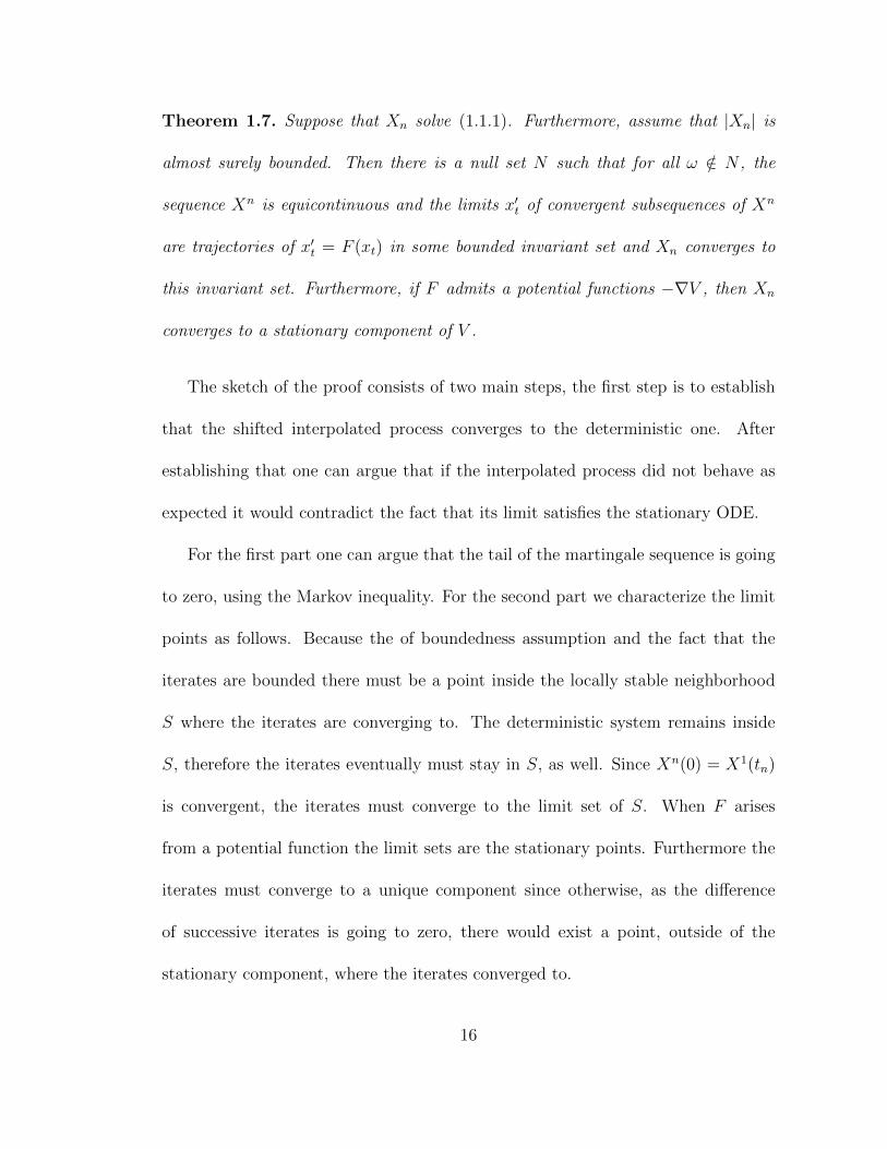
Theorem 1.7. Suppose that Xn solve (1.1.1). Furthermore, assume that |Xn| is
almost surely bounded. Then there is a null set N such that for all ω /∈ N , the
sequence Xn is equicontinuous and the limits x′t of convergent subsequences of Xn
are trajectories of x′t = F (xt) in some bounded invariant set and Xn converges to
this invariant set. Furthermore, if F admits a potential functions −∇V , then Xn
converges to a stationary component of V .
The sketch of the proof consists of two main steps, the first step is to establish
that the shifted interpolated process converges to the deterministic one. After
establishing that one can argue that if the interpolated process did not behave as
expected it would contradict the fact that its limit satisfies the stationary ODE.
For the first part one can argue that the tail of the martingale sequence is going
to zero, using the Markov inequality. For the second part we characterize the limit
points as follows. Because the of boundedness assumption and the fact that the
iterates are bounded there must be a point inside the locally stable neighborhood
S where the iterates are converging to. The deterministic system remains inside
S, therefore the iterates eventually must stay in S, as well. Since Xn(0) = X1(tn)
is convergent, the iterates must converge to the limit set of S. When F arises
from a potential function the limit sets are the stationary points. Furthermore the
iterates must converge to a unique component since otherwise, as the difference
of successive iterates is going to zero, there would exist a point, outside of the
stationary component, where the iterates converged to.
16

In the previous theorem an important assumption was that the iterates were
bounded. When the iterates are not constrained in a bounded domain the analysis
is more complicated. In this case the trajectories can possibly be unbounded, and
stability techniques, a prominent one is establishing the existence of a Liapunov
function, (see [KY03] chapter 5.4) is one of the main ways forward. These methods
can be used to establish that the iterates return to a bounded trajectory infinitely
often, in which case asymptotic analysis techniques similar to Theorem 1.7 can be
utilized.
The main ingredient for the proof of Theorem 1.7 was that the family of the
interpolated process was equicontinuous. In, principle, one can demand minimal
conditions for the step sizes and the stochastic approximation algorithm so that
this property is met. An effort to do that can be seen in [KY03] chapter 5.4,
producing results under weaker conditions. Furthermore, in a certain classes of
problems the conditions specified there can be seen not only being necessary, but
also sufficient.
We have established that the limit of a stochastic approximation is supported
on distinct stationary components. An important next step for the development of
the theory is the investigate which stationary points are limiting. Generally it is
hard to establish whether a saddle point is in the support of X∞, as the underlying
dynamics can lead to very complicated saddle point structures. However, a very
important result [Pem91], shows that when the linearization of F (·) as in (1.1.1),
17

at a point p, has a positive eigenvalue value then p will never be in the support of
X∞.
1.4.4 Motivating example
Here we will revisit Example 1, and the follow up paper of Pemantle [Pem91] which
provides a more detailed description for the support of X∞. The analysis developed
in section 1.4.1 establishes that the support of the limiting process is exactly the set
of fixed points of f (critical points of the corresponding potential). More precisely,
the iterates Xn will avoid local maxima with probability 1, and Xn will converge to
a local minimum with some positive probability. However, at that point in history,
it was unknown whether Xn can converge to saddle points. Later Pemantle, with his
work [Pem91], settled this; giving explicit conditions, and surprisingly depending on
the local behavior of f , the process may or may not converge there. Next, we will
define a quantity which we will need in the next paragraph. Let Zn,m =∑m−1
i=n Yi,
so E(Z2n,m) ≤
∑i≥n
1(i+1)2
∼ 1n. The last equation, after taking m → ∞, is called
the remaining variance for the process Xn, and it measures how much Xn can
potentially deviate from the “mean flow” by the influence of future noise.
We will give the high level intuition, in qualitative terms, utilizing objects al-
ready described, namely the mean flow and the remaining variance. It is clear that
18
the occurrence of convergence or non convergence to a point p, depends on the
behavior of the process Xn when lying in the stable trajectory. Now, for simplicity,
we assume the stable trajectory lies in a left neighborhood of p namely (p − δ, p),
and recalling that p is a saddle point (p, p + δ) realizes the unstable trajectory.
Consequently, assume Xn is moving towards p. The notion of the expected rate
of convergence o1(n) := (Xn − p) can be explicitly computed via solving the mean
flow differential equation. To continue further, as promised, we need to introduce
o2(n) =√E(Z2
n,∞) the order of the square root of the remaining variance. When
o1(n) = o(o2(n)), in every instance where Xn behaves as expected, with h.p. Xn will
be pushed, by the remaining noise, to the unstable trajectory i.e. Xn+k ∈ (p, p+ δ)
for some k > 0. Whenever this happens Xn+k may fail to return to (p− δ, p) with
some positive fixed probability. Finally, by Borel-Cantelli the process will not con-
verge to p with probability 1. Similarly, we can argue that when o2(n) = o(o1(n)),
Xn will converge to p with some positive probability. To elaborate, the probability
that Xn will escape the stable trajectory is decaying rapidly whence by Borel-
Cantelli, in the event that Xn behaves as expected, the process will fail to visit the
unstable trajectory, thereby establishing the convergence of Xn to p.
1.5 Non-convex optimization
Non-convex optimization problems are, generally, NP-hard (for a discussion in the
context of escaping saddle points see [AG16]). The difficulty with high order saddle
19

points can be seen from the fact that it is NP-hard to confirm when a polynomial
of degree 4 is non-negative. We have the following theorem
Theorem 1.8. It is NP-hard to determine whether a homogeneous polynomial of
degree 4 is non-negative.
For a reference see [Nes00] and [HL13]. This limitation does not mean that there
could not exist algorithms that distinguish higher order degenerate saddle points
efficiently when noise is added appropriately into the system. Which in turn could
provide fast convergence to local minima with high probability.
So far, there has been a lot of effort finding fast converging SGD type of al-
gorithms when assuming some non-degeneracy conditions on the Hessian matrix.
Although there are results when the Hessian is degenerate, all the results require
using knowledge of the second order terms (Hessian and higher derivatives) which
are computationally very expensive because they need to calculate the inverse of
the Hessian matrix etc.. So, in practice, they mostly use results that require only
first order information, or at least an oracle calculating the Hessian along one di-
rection. The latter has been shown that it can implemented efficiently by running
a subroutine of a cubic regularization problem [AAZB+17].
One popular condition that guarantees that the SGD will avoid saddle points is
the strict saddle property. Using the terminology of equation (1.1.1), a point p is
a strict saddle when the linearization of F at p contains a positive eigenvalue see
[Pem90] [JGN+17] and [Lev2006]. The paper [Pem90] establishes that if a stochastic
20

approximation satisfies (1.1.1) then it will avoid, asymptotically, a strict saddle
point with probability 1. A result of similar flavor is [LSJR16], where under the same
condition they show that if you randomly initialize GD, then with probability 1 you
avoid strict saddle points. Both of the problems use a stable manifold theorem. The
former result using this decomposition finds a good approximation of the trajectories
in the proximity of the saddle point, and by a change of coordinates it manages to
see how the process gets jiggled in the unstable direction. The latter, via the stable
manifold theorem argues that the set of stable trajectories is of measure zero, hence
if you randomly initialize and then do GD you will avoid the saddle points.
The previous results established some confidence that the first order information
is enough to evade saddle points asymptotically. Next, using the strict saddle
property, in [JGN+17] they managed to evade saddles point with high probability
in O(polylog(d) 1
ε2
)iterations. Here, using again the strict saddle property they
managed to find a novel description of the geometry surrounding a saddle point.
The idea is that when the Hessian has a negative eigenvalue, then only in a small
band parallel to the corresponding eigenvector the process can get stuck. Since
outside of this small band the eigenvector has a dominant effect which forces the
process to decrease rapidly. Using these ideas the algorithm they came up with,
repeats unperturbed gradient descent as long as the gradient is big. When the
gradient is smaller than a certain threshold value they perturb the process, having
in mind, that if the process lands outside the small band the gradient is dominant
21

again. Finally, since, the area of the band is small, with high probability the gradient
will become large so that performing gradient descent is efficient again.
1.6 Further discussion
Here, we will be occupied understanding the support of X∞ in an one dimensional
setting. More specifically, we will work with processes that solve
Xn+1 −Xn =f(Xn)
nγ+Yn+1
nγ, γ ∈ (1/2, 1]. (1.6.1)
To put in the SGD context, the antiderivative of −f would correspond to the
potential function −V . Therefore, if a point p has a neighborhood N such that f
is positive except f(p) = 0, then point p would be a saddle point.
Problem 1. Let (Xn)≥1 solve (1.6.1). Suppose that p is a saddle point. Find the
threshold value:=γ for γ, should it exist, such that:
1. When γ ∈ (1/2, γ), then P(Xn → p) = 0.
2. When γ ∈ (γ, 1], then P(Xn → p) > 0.
Part 1 of Problem 1 guarantees that the SGD avoids saddle points, and hence
converging to local minima. Choosing different γ in the first regime i.e. γ ∈ (1/2, γ),
enables us to optimize SGD’s performance by choosing γ appropriately. In practice
choosing a small step size can slow the rate of convergence, however a bigger step
22

size may lead the process to bounce around (see [BR95] and [SL87]). In [EDM04]
they study the rate of convergence for polynomial step sizes in the context of Q-
learning for Markov decision processes, and they experimentally demonstrate that
for γ approximately 1720
the rate of convergence is optimal.
Here, we are trying to establish that if we understand the underlining dynamical
system sufficiently, then by adding enough noise, the process will wander until it
is captured by a downhill path, and, eventually, will escape the unstable neighbor-
hood. Furthermore, an extension of the results, could, potentially, lead to SGD
type algorithms (in higher dimensions) that converge fast to local minima, even in
the proximity of degenerate saddle points, with high probability.
1.7 Results for the continuous model
We proceed by transitioning to a continuous model. For that purpose we need a
potential, a step size, and a noise term. However, it is natural to consider, without
the need to contemplate, a process defined by
dLt =f(Lt)
tγdt+
1
tγdBt, γ ∈ (1/2, 1]. (1.7.1)
We assume that f(0) = 0, and f is otherwise positive in a neighborhood N of zero.
What we wish to investigate is whether Lt will not converge to 0 with probability
1, or if it will converge there with some positive probability. The answer to these
23

questions depends only on the local behavior of f on N .
The main non-convergence result is the following:
Theorem 1.9. Suppose that N is a neighborhood of zero. Let (Lt)t≥1 be a solution
of (1.7.1), where f(x) is Lipschitz. We distinguish two cases depending on f and
the parameters of the system.
1. k|x| ≤ f(x), k ≥ 12
and γ = 1 for all x ∈ N .
2. |x|k ≤ f(x) , 12
+ 12k≥ γ and k > 1 for all x ∈ N .
If either 1 or 2 holds, then P(Lt → 0) = 0.
In part 1, we have only considered γ = 1 since that is the only critical case,
namely for γ < 1 the effects of the noise would be overwhelming and for all k, we
would obtain P(Lt → 0) = 0.
We now state the main convergence theorem:
Theorem 1.10. Suppose that N is a neighborhood of zero. Let (Lt)t≥1 be a solution
of (1.7.1). We distinguish two cases depending on f and the parameters of the
system.
1. k1|x| ≤ f(x) ≤ k2|x|, 0 < ki < 1/2 and γ = 1 for all x ∈ N ∩ (−∞, 0].
2. 0 < c|x|k ≤ f(x) ≤ |x|k, 12
+ 12k> γ and k > 1 for all x ∈ N ∩ (−∞, 0].
If either 1 or 2 holds, then P(Lt → 0) > 0.
24
This is accomplished by first establishing the previous results for monomials i.e.
f(x) = |x|k or f(x) = k|x|, which is done in sections 3.1, and 3.2. We prove the
stated theorems in section 3.3, by utilizing the comparison results found in section
2.
In section 3.1, we deal with the linear case, i.e. when f(x) = k|x|. There, the
SDE can be explicitly solved, which simplifies matters to a great extent. Firstly,
in subsection 3.1.2, we prove that when k > 1/2, the corresponding process a.s.
will not converge to 0, which is accomplished by proving that it will converge to
infinity a.s.. Secondly, in subsection 3.1.3 we show that process will converge to 0
with some positive probability.
In section 3.2, we move on to the higher order monomials, i.e., f(x) = |x|k.
Here, we show that the process will behave as the “mean flow” process h(t) infinitely
often, which is accomplished by studying the process Lt/h(t). In subsection 3.2.2,
the main theorem is that when 12
+ 12k≥ γ, then Lt →∞ a.s.. In subsection 3.2.3,
we show that when 12
+ 12k< γ holds, the process may converge to 0 with positive
probability.
Qualitatively, the previous constrains on the parameters are in accordance with
our intuition. To be more specific, when k increases, f becomes steeper, which
should indicate it is easier for the process to escape. When γ decreases the remaining
variance increases, hence we should expect that the process visits the unstable
trajectory with greater ease, due to higher fluctuations.
25
1.8 Results for the discrete model
In this section we will state the corresponding results for the discrete model. Fur-
thermore at the end we will provide some examples, and experimental results cor-
roborating the theoretical ones. The asymptotic behavior of the discrete processes
is the expected one, depending on the parameters of the problem. Here, we study
processes satisfying
Xn+1 −Xn ≥f(Xn)
nγ+Yn+1
nγ, γ ∈ (1/2, 1), (1.8.1)
and
Xn+1 −Xn ≤f(Xn)
nγ+Yn+1
nγ, γ ∈ (1/2, 1), (1.8.2)
or
Xn+1 −Xn ≥f(Xn)
n+Yn+1
n, (1.8.3)
and
Xn+1 −Xn ≤f(Xn)
n+Yn+1
n, (1.8.4)
where Yn are a.s. bounded, i.e., there is a constant M such that |Yn| < M a.s.,
E(Yn+1|Fn) = 0, and E(Y 2n+1|Fn) ≥ l > 0. The main non-convergence theorem is
the following
Theorem 1.11. Suppose that N is a neighborhood of zero. We separate two cases
1. Suppose (Xn)n≥1 solve (1.8.1), |x|k ≤ f(x) , 12
+ 12k> γ and k > 1 for all
26

x ∈ N
2. Suppose (Xn)n≥1 solve (1.8.3), k|x| ≤ f(x), k > 1/2 for all x ∈ N
then in both cases P(Xn → 0) = 0.
For the convergence result the non-degeneracy condition E(Y 2n+1|Fn) ≥ l is
replaced with the assumption stated in part 1 of Theorem 1.12.
Theorem 1.12. Let N = (−3ε, 3ε) be a neighborhood of zero. Suppose (Xn)n≥1
solve (1.8.1). We separate two cases
1. There exist −ε2 > −3ε, −ε1 < −ε, such that for all M > 0, there exists
n > M such that P(Xn ∈ (−ε2,−ε1)) > 0.
2. Suppose (Xn)n≥1 solve (1.8.2) 0 < f(x) ≤ |x|k, 12
+ 12k< γ and k > 1 for all
x ∈ N .
3. Suppose (Xn)n≥1 solve (1.8.4) 0 < k|x| ≤ f(x), k > 1/2 for all x ∈ N .
Then when the 1 holds in both cases 2 and 3 we have P(Xn → 0) > 0
The assumption imposed on Xn, part 1 of Theorem 1.12, says that the pro-
cess should be able visit a neighborhood of the origin for large enough n. If this
constraint is not imposed on the process, the previous result need not hold. For
instance, the drift could dominate the noise, and, consequentially, the process may
never reach a neighborhood of the origin with probability 1. There are processes
27
that naturally satisfy this property; such an example is the urn process defined seen
in [Pem91], which is discussed in section 1.4.4.
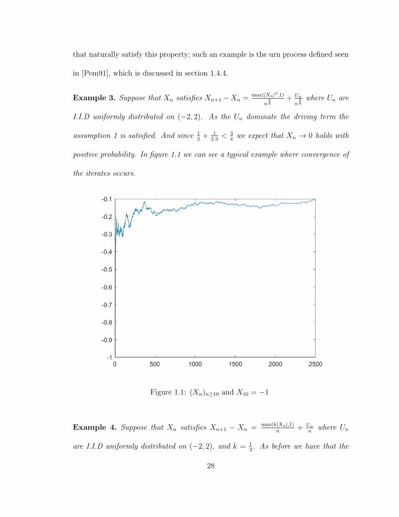
Example 3. Suppose that Xn satisfies Xn+1−Xn = max(|Xn|3,1)n
34
+ Un
n34
where Un are
I.I.D uniformly distributed on (−2, 2). As the Un dominate the driving term the
assumption 1 is satisfied. And since 12
+ 12·3 <
34
we expect that Xn → 0 holds with
positive probability. In figure 1.1 we can see a typical example where convergence of
the iterates occurs.
Figure 1.1: (Xn)n≥10 and X10 = −1
Example 4. Suppose that Xn satisfies Xn+1 − Xn = max(k|Xn|,1)n
+ Unn
where Un
are I.I.D uniformly distributed on (−2, 2), and k = 13. As before we have that the
28

assumption 1 is satisfied. And since k < 12
we expect Xn → 0 to hold with positive
probability. In figure 1.2 we can see a typical example where convergence occurs.
Figure 1.2: (Xn)n≥10 and X10 = −1
Next we will provide some corroborating experimental results. Suppose Xn
satisfies Xn+1 − Xn = f(Xn)nγ
+ Unnγ
where Un are I.I.D uniformly distributed on
(−.5, .5). In the next table we have run simulations in order to investigate whether
Xn converges to 0 or not for various values of γ. The simulations were run for initial
n = 100 and X100 = −1. The criteria for nonconvergence is whether the process at
some point exceeds Xn > 1, at which point the process explodes. The next table is
for the specialization f(x) = |x|3. According to Theorem 1.12 the threshold value
29

for γ is γ = 2/3.
γ iterations nonconv#/100
1 55/100 104 79%
2 55/100 105 100%
3 60/100 104 61%
4 60/100 105 86%
5 70/100 104 4%
6 70/100 105 17%
7 70/100 106 32%
8 70/100 107 38%
The next table is for the specialization f(x) = |x|2. According to Theorem 1.12
the threshold value for γ is γ = 3/4.
γ iterations nonconv#/100
1 60/100 104 91%
2 60/100 105 100%
3 70/100 104 33%
4 70/100 105 68%
5 70/100 106 94%
6 78/100 104 0%
7 78/100 105 1%
8 78/100 106 8%
30

Next we will provide a similar analysis for the linear case, i.e., when f(x) = k|x|
and γ = 1. Here, we have a threshold value for k, namely k = 1/2.
k iterations nonconv#/100
1 1 104 21%
2 1 105 64%
3 1 106 79%
4 2/5 104 0%
5 2/5 105 3%
6 2/5 106 6%
31

1.9 Further conjectures
Suppose that (Xn)n≥1 satisfies (1.1.1), where F = −∇V and an = 1nγ
. Here,
V : Rd → R is an analytic function, such that V (0) = ∇V (0) = 0. Hereby, we
assume that 0 is a saddle point that it is, also, an isolated critical point.
For this section we will focus on problem 1 part (1). More specifically, the goal
is to find γ ∈ (1/2, 1] such that P(Xn → 0) = 0. We will start by discussing about a
potential strategy for a generic analytic function F which arises from some potential
function V . Then we will provide specific examples.
One of the main tools we will need, for the initial discussion, is a Lojasiewicz
type inequality, for a reference see [Spr], Theorem 2 and [Son12], Lemma 3.2, page
315.
Definition 1.13. Suppose that V : Rn → R. Then denote the zero set of V by
ZV = x ∈ Rn : V (x) = 0.
Theorem 1.14. Let V be defined as before. Let ZV denote the zero set of V . Then,
there is an open set 0 ∈ O such that there is a positive constant k ∈ (1, 2) such that
the following holds:
(a) |∇V (x)| ≥ c|V (x)|k/2 for all x ∈ O.
The line of attack consists of three distinct steps.
• We start by studying the process (V (Xn))n≥1. Using Theorem 1.14 we get an
upper bound on the |V (Xn)|.
32
• Then the process Xn may wander into the realm where V (Xn) < 0 with
probability bounded from below.
• Lastly, we show that when V (Xn) < 0, the process may stay negative with
probability bounded from below, hence concluding that P(Xn → 0) = 0.
For the first step using Theorem 1.14, part (a) we see that Yn := V (Xn) satisfies a
recursion similar to the ones in section 1.8, namely
Yn+1 − Yn = −|Yn|k
nγ+
Noisen+1
nγ+ O
(1
n2γ
), (1.9.1)
where the noise satisfies E(Noise2n+1|Fn
)≥ |Yn|k. Proof of equation (1.9.1): We
expand V centered at Xn and we obtain
V (Xn+1)− V (Xn) = ∇V (Xn) · (Xn+1 −Xn) +M ||Xn+1 −Xn||2
≤ −||∇V (Xn)||2
nγ+∇V (Xn) ·Bn+1
nγ+
1
n2γ
< −|V (Xn)|k
nγ+∇V (Xn) ·Bn+1
nγ+
1
n2γ
Now, using that the noise is quasi-isotropic we see that the new noise satisfies
E((∇V (Xn) ·Bn+1)2|Fn) = E((
∇V (Xn)
||∇V (Xn)||·Bn+1)
2||∇V (Xn)||2|Fn)
= E((∇f(vn)
||∇V (Xn)||·Bn+1)
2|Fn)||∇V (Xn)− V (0)||2
≥ 1 · |V (Xn)|k.
33

The recursion defined in equation (1.9.1), can provide an upper bound |V (Xn)|,
however this could be far from optimal as we have the bias term 1n2γ that we need
take into account.
For the second part of the strategy we notice that the path from Xn to z ∈ ZV ,
along the flow x′t = −∇V (xt) has length V (Xn). So, we should expect that as long
as V (Xn) and the remaining noise in the recursion (1.1.1) are comparable, then Xn
may wander in the realm where V (Xn) < 0.
Definition 1.15. Suppose that V : Rn → R and let x ∈ Rn such that V (x) < 0.
Denote by Ox the connected component of x ∈ Rn : V (x) ≤ 0 such that x ∈ Ox.
For the last step of the strategy we ought to understand the geometry of the
conical region OXn ∩ ZV . For instance the surface OXn ∩ ZV can be very steep
so that under the slightest perturbation the iterate Xn may return to the realm
V (Xn) > 0.
Example 5. Suppose that V (x, y) = x4 + x2y2 − y4, that is V is a homogeneous
polynomial of degree 4. Then since V (r~x) = r4V (~x), we see that O~y ∩ZV is a cone
for any ~y such that V (~y) < 0. Define Wn = (Xn, Yn) given by
Wn+1 −Wn =∇V (Wn)
nγ+Bn+1
nγ
where for simplicity we assume that Bn+1 = (U1,n+1, U2,n+2) where Ui,n for i = 1, 2
and n ∈ N is a collection of independent uniforms on (−1, 1). Now, we may write
34
the recursion for Xn and Yn, namely
Xn+1 −Xn =−4X3
n − 2XnY2n
nγ+N1,n+1
nγ(1.9.2)
and
Yn+1 − Yn =−4Y 3
n + 2X2nYn
nγ+N2,n+1
nγ(1.9.3)
Using symmetry we may assume that Xn > 0. Under this assumption we obtain the
following bound
Xn+1 −Xn ≤−4X3
n
nγ+N1,n+1
nγ.
Therefore, by Theorem 4.1 it is always possible to choose γ such that Xn crosses 0.
From here, we can see that the process Wn will eventually land with probability 1 in
the realm V (Wn) < 0.
Example 6. Suppose that V (x, y) = x6 + x2y2 − y6. Here the conical surface is
similar to the surface y =√|x|. However, even though the region Oy is very steep,
see figure 1.3, simulations suggest that for certain values of γ the process defined by
Xn+1 −Xn =∇V (Xn)
nγ+Yn+1
nγ,
will not get stuck along a stable trajectory, i.e., P(Xn+1 → 0) = 0.
35

In the simulations the parameter γ was set γ = .6.
Figure 1.3: Vector flow
36

Chapter 2
Preliminary results
We will now prove two important lemmas that will be needed throughout. Let
f : R→ R, be Lipschitz such that for all ε > 0 there exists c such that f(x) > c > 0,
for all x ∈ R\ (−ε, ε). Also, we define a continuous function g : R≥0 → R, such that∫∞0g2(t)dt <∞. Let Xt satisfy
dXt = f(Xt)dt+ g(t)dBt. (2.0.1)
Lemma 2.1. lim supt→∞Xt ≥ 0 a.s..
Proof: We will argue by contradiction. Assume that lim supt→∞Xt < 0, and
pick δ > 0 such that lim supt→∞Xt < −δ with positive probability. Then there is a
time u, such that Xt ≤ −δ for all t ≥ u. But this has as an immediate consequence
that∫ t1f(Xs)ds → ∞. However, since the process Gt =
∫ t1g(s)dBs has finite
quadratic variation, i.e., supt〈Gt〉 =∫∞0g2(t)dt <∞, Gt stays a.s. finite. The last
37

two observations imply that Xt →∞, which is a contradiction.
Lemma 2.2. lim inft→∞Xt ≥ 0 a.s..
Proof: We will again argue by contradiction. Assume that lim inft→∞Xt < 0
on a set of positive probability. Take an enumeration of the pair of positive rationals
(qn, pn) such that qn > pn. Now, define An = Xt ≤ −qn i.o., Xt ≥ −pn i.o.. Since
lim supt→∞Xt ≥ 0, we have⋃n≥0An = lim inft→∞Xt < 0. Now, for t1 < t2
assume that Xt1 ≥ −pn and Xt2 ≤ −qn. Then, we see that Xt2 −Xt1 ≤ −qn + pn,
however
Xt2 −Xt1 =
∫ t2
t1
f(Xs)ds+
∫ t2
t1
g(s)dBs
≥∫ t2
t1
g(s)dBs.
Hence we conclude that∫ t2t1g(s)dBs ≤ −qn + pn. By the definition of An, on
event An we can find a sequence of times (t2k, t2k+1) such that t2k < t2k+1 and∫ t2k+1
t2kg(s)dBs ≤ −qn + pn. Now, if we define Gu,t =
∫ tug(s)dBs, we see that
G1,t converges a.s. since it is a martingale of bounded quadratic variation. Hence
P(An) = 0, i.e., P(lim inft→∞Xt < 0) = 0.
The next comparison result is intuitively obvious, however, it will be useful for
comparing processes with different drifts.
Proposition 2.3. Let (Ct)t≥0 and (Dt)t≥0 stochastic processes in the same Wiener
space, that satisfy dCt = f1(Ct)dt+ g(t)dBt, dDt = f2(Dt)dt+ g(t)dBt respectively,
38
where g, f1, f2 are deterministic real valued functions. Assume that f1(x) > f2(x)
for all x ∈ R and Cs0 > Ds0, then Ct > Dt∀t ≥ s0 a.s..
Proof: Define τ = infτ > s0|Cτ = Dτ, and setDτ = Cτ = c, for τ <∞. Now,
from continuity of f1, and f2 we can find δ such that f1(x) > f2(x),∀x ∈ (c− δ, c].
However, for all s we have Cτ−Dτ−(Cs−Ds) = −(Cs−Ds) =∫ τsf1(Cu)−f2(Du)du.
Thus, for s such that Cy, Dy ∈ (c− δ, c)∀y ∈ (s, τ) we have
0 > −(Cs −Ds)
=
∫ τ
s
f1(Cu)− f2(Du)du
> 0.
Therefore, τ <∞ has zero probability.
In what follows, we will prove two important lemmas, corresponding to Lemma
2.1 and Lemma 2.2, for the discrete case. We will assume that Xn satisfies
Xn+1 −Xn ≥f(Xn)
nγ+Yn+1
nγ, γ ∈ (1/2, 1) (2.0.2)
where f satisfies ∀ε > 0,∃c > 0, f(x) ≥ c, x ∈ (−∞,−ε), and the Yn are defined
similarly, as in (1.8.1).
Lemma 2.4. lim supXn ≥ 0 a.s..
Proof: The proof is nearly identical as in the continuous case (Lemma 2.1).
39

Lemma 2.5. lim inft→∞Xt ≥ 0 a.s..
Proof: The proof is identical as in the continuous case (Lemma 2.2).
We provide a suitable version of the Borel-Cantelli lemma (for a reference see
Theorem 5.3.2 in [Dur13]).
Lemma 2.6. Let Fn, n ≥ 0 be a filtration with F0 = 0,Ω, and An, n ≥ 1 a
sequence of events with An ∈ Fn. Then
An i.o. =
∑n≥1
P(An|Fn−1) =∞
.
40
Chapter 3
Continuous model
3.1 Continuous model, simplest case
3.1.1 Introduction
Let Lt be defined by (1.7.1), for f(x) = k|x| and γ = 1. To simplify, we make a
time change and consider Xt := Let , and subsequently we obtain,
Xt+dt −Xt = Let+etdt − Let
= k|Let |dt+ e−t(Bt+etdt −Bet)
= k|Xt|dt+ e−t2 dBt.
41

Which will be the model we will study. We begin with some definitions.
dXt = k|Xt|dt+ e−t2 dBt. (3.1.1)
We introduce another SDE closely related to the previous one, which will be useful.
dKt = kKtdt+ e−t2 dBt. (3.1.2)
It is easy to see that both of these SDEs admit unique strong solutions, for a
reference see theorem (11.2) in chapter 6 in [RWW87]. Therefore, we can construct
Xt, Kt in the classical Wiener space (Ω,F ,P). The solution for SDE (3.1.2), is
given by Kt = ekt(e−t0kKt0 +∫ tt0e−s(k+
12)dBs). Indeed, substituting in (3.1.2), and
using Ito’s formula we get
dKt = a′(t)(k0 +
∫ t
t0
b(s)dBs) + a(t)b(t)dBt
=a′(t)
a(t)Kt + a(t)b(t)dBt.
Where a(t) = ek(t−t0), and b(t) = e−t(12+k)+kt0 . Therefore, a′(t)
a(t)= k, a(t)b(t) = e−
t2 ,
so we conclude.
Proposition 3.1. Let (Xt)t≥t0 , (Kt)t≥t0 in the Wiener probability space (Ω,F ,P)
be the solutions of (3.1.1),(3.1.2) respectively. We start them at time t0, Xt0 ≥
Kt0 ≥ 0. Then Xt ≥ Kt, ∀t ≥ t0.
42

It is a direct application of Proposition 2.3.
3.1.2 Analysis of Xt when k ≥ 1/2.
We start by stating the main result of this subsection, which we will prove at the
end of the subsection.
Theorem 3.2. Let (Xt)t≥1 the solution of (3.1.1) for k ≥ 12, then Xt →∞ a.s..
We will prove the theorem at the end of the subsection. Now, we will show that
(Xt)t≥1 cannot stay negative for all times. This will be accomplished by a direct
computation, after solving the SDE.
Proposition 3.3. Let (Xt)t≥1 the solution of (3.1.1) for k > 12. Assume that at
time s, Xs < 0, then Xt will reach 0 with probability 1, i.e. P(supu≥sXu > 0) = 1
Proof: First, note that the solution of the SDE (3.1.1), run from time s with
initial condition Xs < 0 coincides with the solution of the SDE dXt = −kXtdt +
e−t2 dBt before Xt hits 0. Formally, we define τ0 = inft|t ≥ s, Xt = 0. Using the
same method when solving SDE (3.1.2), we obtain Xt = e−kt(eksXs+∫ tseu(k−
12)dBu),
on t < τ0. First we deal with the case k 6= 12. Set Gt =
∫ tseu(k−
12)dBu, and
calculate the quadratic variation of Gt, namely 〈Gt〉 = (e2t(k−12)−e2s(k− 1
2))/(2k−1).
43
Next, we compute the probability of never returning to zero.
P(τ =∞) = P(
sups<u<∞
Xu ≤ 0
)= P
(sup
s<u<∞Gu ≤ −eksXs
)= 1− P
(sup
s<u<∞Gu > −eksXs
)= 1− lim
t→∞P(
sups<u<t
Gu > −eksXs
)= 1− lim
t→∞2P(Gt > −eksXs
), from the reflection principle
= 1− limt→∞
2P
(N
(0,e2t(k−
12) − e2s(k− 1
2)
2k − 1
)> −eksXs
)
= 0, sincee2t(k−
12) − e2s(k− 1
2)
2k − 1→∞
When k = 12, the solution simplifies to Xt = e−kt(eksXs + Bt) in distribution,
where Btt≥s with initial condition Bs = 0. We repeat the previous calculation,
P(τ =∞) = P(
sups<u<∞
Xu ≤ 0
)= P
(sup
s<u<∞Bu ≤ −eksXs
)= 0
as for a Brownian motion we have lim supt→∞Bt =∞ almost surely.
We will now prove two important lemmas, that are true for solutions of (3.1.1)
for any k > 0.
44

Lemma 3.4. Let (Xt)t≥1 the solution of (3.1.1). Then on the event Xt ≥ 0 i.o.,
there is a positive constant c < 1 such that Xt ≥ ce−t/2 i.o. holds a.s..
Proof: Assume we start the SDE at time ti with initial condition Xti ≥ 0. Then
we see that Xt ≥∫ ttik|Xu|du+
∫ ttie−
u2 dBu ≥
∫ ttie−
u2 dBu.
Set Gt =∫ ttie−
u2 dBu. The quadratic variation of Gt, is 〈Gt〉 = e−t1 − e−t.
Fix 0 < c < 1. Now, observe that we can always choose t big enough such that
〈Gt〉 ≥ ce−t1 for any t1.
Then,
P( supti<u<t
Xt > e−t1/2) ≥ P( supti<u<t
Gt > e−t1/2)
= 2P(Gt > e−t1/2)
≥ 2P(N(0, ce−t1) > e−t1/2)
= 2P(N(0, c) > 1) > γ > 0.
Let g(x) = infy|e−x − e−y ≥ ce−x. Now, we can formally define the sequence of
the stopping times. The first stopping time is τ1 = inft|Xt ≥ 0, then we define
recursively τi+1 = inft|t > τi, t > g(τi), Xt ≥ 0. We, also, define the associated
filtration Fn = Fτn , for n ≥ 1 and F0 = 0,Ω. Now, let An = ∃t, τn−1 <
t < τn , s.t. Xt ≥ ce−t/2. So, by definition An ∈ Fn. We find a lower bound for
45

P(An|Fn−1).
P(An|Fn−1) ≥ P( supτn−1<u<τn
Xu > ce−tn−1/2|Fn−1)
≥ P( supτn−1<u<g(tτn−1)
Xu > ce−τn−1/2|Fn−1)
> γ.
On Xt ≥ 0 i.o. the sum∑
n≥1 P(An|Fn−1) has infinite non zero terms bigger than
γ, hence∑
n≥1 P(An|Fn−1) = ∞ a.s.. Finally, by Lemma 2.6 (Borel-Cantelli) we
conclude.
The next lemma uses the previous lemma to establish that on Xt ≥ 0 i.o. we
have lim inft→∞Xt > 0.
Lemma 3.5. Let (Xt)t≥1 the solution of (3.1.1). Then on the event Xt ≥ 0 i.o.
we have that lim inft→∞Xt > 0 holds a.s..
Proof: Indeed, if we start the process at time s with initial condition Xs ≥ ce−s2 ,
then the solution of (3.1.1), before hitting 0, is given by
Xt = ekt(e−ksXs +
∫ t
s
e−u(k+12)dBu
)≥ ekt
(ce−s(k+
12) +
∫ t
s
e−u(k+12)dBu
).
Denote Gt =∫ tse−s(k+
12)dBs. We calculate its quadratic variation
〈Gt〉 =e−2tk−t
−2k − 1+e−2sk−s
2k + 1.
46

Taking t→∞, shows 〈G∞〉 =e−2sk−s
2k + 1. Therefore,
P( infs≤u<∞
Xu >c
2e−
s2 ) = P( inf
s≤u<∞eku(ce−s(k+
12) +Gu) >
c
2e−
s2 )
≥ P( infs≤u<∞
eks(ce−s(k+12) +Gu) >
c
2e−
s2 )
= P( infs≤u<∞
ce−s(k+12) +Gu >
c
2e−s(k+
12))
= P( infs≤u<∞
Gu > −c
2e−s(k+
12)) (3.1.3)
= 1− P( sups≤u<∞
Gu >c
2e−s(k+
12))
= 1− 2 limt→∞
P(Gt > −c
2e−s(k+
12)), by the reflection principle
= 1− 2P(N(0,e−s(2k+1)
2k + 1) >
c
2e−s(k+
12))
= 1− 2P(N(0,1
k + 1) >
c
2) > δ > 0.
We know that on Xt ≥ 0 i.o. the event Xt ≥ ce−t2 i.o. holds a.s.. Therefore, on
Xt ≥ 0 i.o., if we define τ0 = 0, and τn+1 = t > τn + 1|Xt ≥ ce−t2 we see that
τn <∞ a.s., and τn →∞ a.s.. Also, we define the corresponding filtration, namely
Fn = σ(τn).
To show that on the event Xt ≥ ce−t2 i.o. the event A = lim inf→∞Xt ≤ 0
has probability zero, it suffices to argue that there is a δ such that P(A|Fn) < 1−δ,
47
a.s. for all n ≥ 1. This is immediate from the previous calculation. Indeed,
P(A|Fn) ≤ 1− P( infτn≤u<∞
Xu >c
2e−
τn2 |Fn)
< 1− δ.
Now, we can prove Theorem 3.2.
Proof of Theorem 3.2: From Proposition 3.3 we know that Xt ≥ 0 i.o.
has probability 1. Therefore, from Lemma 3.5 we deduce lim inft→∞Xt > 0 almost
surely. Consequently,∫∞0|Xu|du→∞ a.s.. At the same time lim supt→∞
∫ t0e−
u2 dBu <
∞ a.s., hence Xt →∞ a.s..
3.1.3 Analysis of Xt when k < 1/2.
As before, (Xt)t≥1 is the solution of the stochastic differential equation dXt =
k|Xt|dt + e−t2 dBt.
The behavior of Xt, when k < 1/2 is different. The process in this regime can
converge to 0 with positive probability. More specifically, we have the following
theorem:
Theorem 3.6. Let (Xt)t≥1 solve (3.1.1) with k < 12, and define A = Xt → 0,
B = Xt →∞. Then the following hold:
1. Let A,B as before. Then P(A ∪B) = 1.
48

2. Both A and B are non trivial, i.e., P(A) > 0 and P(B) > 0.
3. On Xt ≥ 0 i.o. we get Xt →∞.
Before proving the theorem, we need to prove a proposition first. We will show
that that the process, starting from a negative value, will never cross 0 with positive
probability.
Proposition 3.7. Let (Xt)t≥1 solve (3.1.1) with k < 12. Assume that at time s,
Xs < 0. Then (Xt)t≥1 will hit 0 with probability α where 0 < α < 1.
Proof: Define the stopping time τ1 = inft ≥ s|Xt = 0. As in Proposition 3.3,
the solution for Xt started at time s up till time τ1, is given by Xt = e−kt(eksXs +∫ tseu(k−
12)dBu).
P(τ =∞) = P( sups<u<∞
Xu ≤ 0)
= 1− limt→∞
2P(N(0,e2t(k−
12) − e2t(k− 1
2)
2k − 1) > −eksXs), as in Proposition 3.3
= 1− 2P(N(0,−e2s(k−12)/(2k − 1)) > −eksXs) = 1− α.
Therefore 0 < α < 1.
Proof of Theorem 3.6:
1. Define the events N = ∃s, s.t.Xt < 0∀t ≥ s, and P = Xt ≥ 0 i.o.. Of
course N and P are disjoint and P(P ∪N) = 1. To prove 1, we will show that
N ⊂ Xt → 0 up to a null set and P = Xt →∞.
49
From Lemma 2.2 we know that lim inft→∞Xt ≥ 0 a.s., therefore on N ⊂
Xt → 0 up to a null set.
To show that P = Xt → ∞, note that Lemma 3.5 shows that on Xt ≥
0 i.o., lim inft→∞Xt > 0 almost surely. Consequently, on Xt ≥ 0 i.o., we
have Xt → ∞, as∫∞0|Xu|du → ∞ and lim supt→∞
∫ t0e−
u2 dBu < ∞ a.s..
Therefore, P = Xt →∞. Which concludes part 1.
2. The fact that P(A) > 0, follows immediately from Proposition 3.7. Now, we
will prove that P(B) > 0. Define the stopping time τ0 = inft|Xt = 0. Also,
define Y (t, ω) = 1 if Xs ≥ 0 for all s ≥ t + 1. Observe that Yτ0 = 1, τ0 <
∞ ⊂ P . Hence, using the strong Markov property
P(Yτ = 1, τ <∞) =
∫ ∞0
P(τ = u)P0(Xt ≥ 0,∀t ≥ 1)du
≥∫ ∞0
P(τ = u)P0(Kt ≥ 0,∀t ≥ 1)du since Xt ≥ Kt
= αP0(Kt ≥ 0,∀t ≥ 1) > 0.
3. Follows immediately from the proof of 1.
Lastly, we prove a proposition that will be used in section 3.3.
Proposition 3.8. Suppose (Xt)t≥1, (Yt)t≥1 solve (3.1.1), with constants k and k1
respectively. Suppose, that 0 < k1 < k < 1/2. Let ε > 0, if Xs, Ys ∈ (−2ε,−ε)
50
a.s., then there is an event A with positive probability, such that both Xt, Yt ∈
(−3ε, 0), ∀t > s.
Proof: Solving the SDE before it hits zero we find, Xt = e−kt(eksXs+∫ tseu(k−
12)dBu)
and Yt = e−k1t(ek1sYs +∫ tseu(k1−
12)dBu). Let ε > 0. Since, the process Gt =∫ t
seu(k−
12)dBu has finite quadratic variation, the event A = Gt ∈ (−ε, ε) ∀t > s
has positive probability. Set Gt =∫ tseu(k1−
12)dBu, and define Nt = Gte
t(k1−k). Using
Ito’s formula, we find dNt = et(k−12)e(k1−k)tdBt + (k1 − k)e(k1−k)tGtdt. Therefore,
Gte(k1−k)t = Gt +
∫ t
s
(k1 − k)e(k1−k)uGudu.
So,
Gte(k1−k)t −
∫ t
s
(k1 − k)e(k1−k)uGudu = Gt.
To bound |Gt| observe that
−∫ t
s
(k1 − k)e(k1−k)uGudu ≤ −ε∫ t
s
(k1 − k)e(k1−k)udu
= −ε(e(k1−k)t − e(k1−k)s
)
Similarly we obtain −∫ ts(k1 − k)e(k1−k)uGudu ≥ ε
(e(k1−k)t − e(k1−k)s
). Thus on A,
we obtain the following inequalities
−εe(k1−k)t + ε(e(k1−k)t − e(k1−k)s
)≤ Gt ≤ εe(k1−k)t − ε
(e(k1−k)t − e(k1−k)s
).
51

Simplifying, we obtain |Gt| ≤ εe(k1−k)s ≤ ε. Now, we will estimate Xt on A. Using
that ε < |eksXs| we obtain the following upper bound,
Xt = e−kt(eksXs +
∫ t
s
eu(k−12)dBu
)≤ e−kt
(eksXs + ε
)< 0.
and lower bound
Xt = e−kt(eksXs +
∫ t
s
eu(k−12)dBu
)≥ e−kt(−2eksε− ε)
≥ −3ε.
Doing similarly for Yt, we conclude.
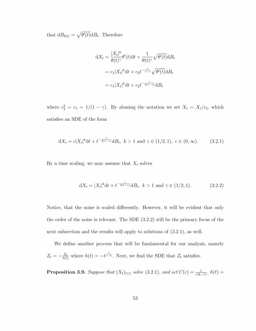
3.2 Analysis of dLt =|Lt|ktγ dt + 1
tγdBt.
3.2.1 Introduction
As in the previous section, to simplify matters, we will work with reparametrizing
Lt. Set θ(t) = t1
1−γ , and let Xt = Lθ(t). To obtain the SDE that Xt obeys, notice
52
that dBθ(t) =√θ′(t)dBt. Therefore
dXt =|Xt|k
θ(t)γθ′(t)dt+
1
θ(t)γ
√θ′(t)dBt
= c1|Xt|kdt+ c2t− γ
1−γ√θ′(t)dBt
= c1|Xt|kdt+ c2t− γ
2(1−γ) dBt
where c22 = c1 = 1/(1 − γ). By abusing the notation we set Xt = Xt/c2, which
satisfies an SDE of the form
dXt = c|Xt|kdt+ t−γ
2(1−γ) dBt, k > 1 and γ ∈ (1/2, 1), c ∈ (0,∞). (3.2.1)
By a time scaling, we may assume that Xt solves
dXt = |Xt|kdt+ t−γ
2(1−γ) dBt, k > 1 and γ ∈ (1/2, 1). (3.2.2)
Notice, that the noise is scaled differently. However, it will be evident that only
the order of the noise is relevant. The SDE (3.2.2) will be the primary focus of the
next subsection and the results will apply to solutions of (3.2.1), as well.
We define another process that will be fundamental for our analysis, namely
Zt = − Xth(t)
where h(t) = −t1
1−k . Next, we find the SDE that Zt satisfies.
Proposition 3.9. Suppose that (Xt)t≥1 solve (3.2.1), and set C(c) = 1c(k−1) , h(t) =
53

−t1
1−k . Then, the process Zt = − Xth(t)
satisfies
Zt − Zs =
∫ t
s
cXu
h(u)
(C|h(u)|k
h(u)− |Xu|k
Xu
)du+
∫ t
s
− 1
h(u)u−
γ2(1−γ) dBu. (3.2.3)
Also, before Xt hits zero we get a solution purely in terms of Zt,
Zt − Zs =
∫ t
s
c|h(u)|k−1Zu(C − (−Zu)k−1
)du+
∫ t
s
− 1
h(u)u−
γ2(1−γ) dBu. (3.2.4)
Proof: Recall that since h(t) is a continuous function, the covariance 〈h(t), Zt〉 =
0. Using Ito’s formula we obtain
dZt = − 1
h(t)dXt +Xtd
(− 1
h(t)
).
Thus,
Zt − Zs =
∫ t
s
− 1
h(u)c|Xu|kdu+
∫ t
s
− 1
h(u)u−
γ2(1−γ) dBu +
∫ t
s
Xuh′(u)
h(u)2du
=
∫ t
s
Xuh′(u)
h(u)2− 1
h(u)c|Xu|kdu+
∫ t
s
− 1
h(u)u−
γ2(1−γ) dBu
=
∫ t
s
cXu
h(u)
(h′(u)
ch(u)− |Xu|k
Xu
)du+
∫ t
s
− 1
h(u)u−
γ2(1−γ) dBu
=
∫ t
s
cXu
h(u)
(1
c(k − 1)
|h(u)|k
h(u)− |Xu|k
Xu
)du+
∫ t
s
− 1
h(u)u−
γ2(1−γ) dBu.
The SDE (3.2.4) is an immediate consequence of the last line of the previous calcu-
lation.
54

In the next proposition, we describe some properties of the noise for the process
Zt, and give a very important inequality for subsection 3.2.2, which relates the order
of the deterministic system converging to zero and order of the remaining noise for
Xt, i.e., the order of 〈∫∞su−
γ2(1−γ) dBu〉.
Proposition 3.10. Set G′s,t =∫ ts− 1h(u)
u−γ
2(1−γ) dBu, the noise term of (3.2.4) and
(3.2.3).
1. In the regime 12
+ k2≥ γ, 〈G′s,∞〉 =∞
2. In the regime 12
+ k2< γ, 〈G′s,∞〉 <∞
3. Also, given the same conditions as in part 1 for the pair (k, γ), the following
inequality is true
1
k − 1≥ 2γ − 1
2(1− γ)
Proof: We calculate its quadratic variation at time t, namely, 〈G′s,t〉 =∫ ts
1h(u)2
u−γ
(1−γ) du.
Notice that by the definition of h(t), we have h(t)−1 = Θ(t1
k−1 ), therefore− 1h(u)2
u−γ
(1−γ) =
Θ(u2
k−1− γ
1−γ ). Consequently, 〈G′s,∞〉 =∞ when
2
k − 1− γ
1− γ≥ −1 ⇐⇒ 2
k − 1+
1
γ − 1≥ −2.
55

In the first regime we have,
1
2+
1
2k≥ γ ⇐⇒ k − 1
2k≤ 1− γ ⇐⇒ 2k
k − 1≥ 1
1− γ
⇐⇒ 2
k − 1+ 2 ≥ 1
1− γ⇐⇒ 2
k − 1+
1
1− γ≥ −2 (3.2.5)
So, indeed, when 12
+ 12k≥ γ, 〈G′s,∞〉 =∞. Also, from the previous calculation we
see that when 12
+ 12k< γ then 2
k−1−γ
1−γ < −1, therefore when 12
+ 12k< γ, 〈G′s,t〉 <
∞. Finally, rearranging the first inequality of (3.2.5) we obtain 1k−1 ≥
2γ−12(1−γ) .
The solution of the SDE (3.2.2), when Xt is positive, explodes in finite time.
However, since we are interested in the behavior of Xt when Xt < M for a positive
constant M , we may change the drift when Xt surpasses the value M , which in turn
it would imply that SDE (3.2.2) admits strong solutions. One way to do this is by
studying the SDE whose drift term is equal to |x|k when |x| < M and M when
|x| > M . This SDE can be seen to admit strong solutions for infinite time. The
reason is that this process Xt is a.s. bounded from below, as the drift is positive.
Also, Xt cannot explode to plus infinity in finite time since the drift is bounded
from above when Xt is positive. However, for simplicity, we will use the form as
shown in (3.2.2).
3.2.2 Analysis of Xt when 1/2+1/2k ≥ γ, k > 1 and γ ∈ (1/2, 1)
The main result of this subsection is the following theorem.
56

Theorem 3.11. Let (Xt)t≥1, that solves (3.2.2). When 1/2 + 1/2k ≥ γ,Xt → ∞
a.s.
We will see its proof at the end of the subsection. Now, we will prove an
important proposition, which shows that Xt cannot stay far away from the left of
the origin.
Proposition 3.12. Let (Xt)t≥1 solve (3.2.1) for c = 1. Then, for some β < 0, the
event Xt ≥ βt1−2γ2(1−γ) i.o. has probability 1.
Proof: Set G′t =∫ ts− 1h(u)
u−γ
2(1−γ) dBu, which corresponds to the noise term
of (3.2.4). First, we will prove that Xt ≥ C ′h(t), i.o. a.s., where C ′ > C1
k−1
and C = C(1) = 1k−1 . To do so, we will argue by contradiction. Assume that
A = ∃ s,Xt < C ′ · h(t)∀t > s has positive measure. Take ω ∈ A, and find s(ω)
such that Xt < C ′ · h(t) for all t > s. Notice, that this implies that Zt < −C ′ for
t > s. Take u > s, since |x|k
xis increasing we see that |Xu|
k
Xu< C ′k−1 |h(u)|
k
h(u)< C |h(u)|
k
h(u).
This in turn gives C |h(u)|k
h(u)− |Xu|
k
Xu> 0. Therefore
∫ ts
Xu
h(u)
(C |h(u)|
k
h(u)− |Xu|
k
Xu
)du > 0
for all t > 0. However, since G′w,t :=∫ tw− 1h(u)
u−γ
2(1−γ) dBu for any fixed w has infinite
quadratic variation, we may find G′s,t > −Zs. Now, from (3.2.3) we get
Zt =
∫ t
s
Xu
h(u)
(C|h(u)|k
h(u)− |Xu|k
Xu
)du+ Zs +G′s,t
> 0.
This contradicts the fact that Zt < −C ′. Therefore Xt > C ′h(t), i.o. a.s.
57

Finally, in Proposition 3.10 part 3 we have shown that 1k−1 ≥
2γ−12(1−γ) , therefore
−t1
1−k ≥ −t1−2γ2(1−γ) . So, we conclude that there exists a constant β < 0 such that
Xt ≥ βt1−2γ2(1−γ) i.o. holds a.s.
Corollary 3.13. Let (Xt)t≥1 solve (3.2.1) for c = 1. Then lim inft→∞Xt > 0
almost surely.
Proof: Set Gs,t =∫ tsu−
γ2(1−γ) dBu and note that 〈Gs,∞〉 = Θ(s
1−2γ(1−γ) ). Fix γ > 0,
since 〈Gs,∞〉 = Θ(s1−2γ(1−γ) ) for any u > 0, it is possible to find by using the reflection
principle W (u) > u > 0 such that
P
(sup
u<t<W (u)
Gu,t > γu1−2γ2(1−γ)
)> δ, (3.2.6)
for δ independent of u. Take γ > −β, where β is such that Xt ≥ βt1−2γ2(1−γ) i.o. (as
in Proposition 4.3). Now, using the lower bound Xt −Xs ≥ Gs,t, we obtain
P
(sup
s<t<W (s)
Xt −Xs > γs1−2γ2(1−γ)
)≥ P
(sup
s<t<W (s)
Gs,t > γs1−2γ2(1−γ)
)> δ. (3.2.7)
When Xs ≥ βs1−2γ2(1−γ) observe that on the event sups<t<W (s)Xt − Xs > γs
1−2γ2(1−γ)
there is τs such that Xτs ≥ Xs + βs1−2γ2(1−γ) = (γ + β)s
1−2γ2(1−γ) ≥ 0. Hence, if we choose
a sequence of stopping times such that Xτn ≥ βτn1−2γ2(1−γ) and τn+1 > W (τn), we have
P(supτn<t<τn+1Gτn,t > γτn
1−2γ2(1−γ) |Fτn) > δ. So, by Borel-Cantelli (Lemma 2.6) on
the events supτn<t<τn+1Xt −Xτn > γτ
1−2γ2(1−γ)n we may conclude that Xt ≥ 0 i.o.
has probability 1. Define τn as before, except that instead of Xτn ≥ βτn1−2γ2(1−γ) we set
58

Xτn ≥ 0, by Borel-Cantelli we obtain that Xt ≥ γt1−2γ2(1−γ) i.o. has probability 1.
Since Gs,t is symmetric and 〈Gs,∞〉 = Θ(s1−2γ(1−γ) )
P( infs<t<∞
Xt −Xs > −γ
2s
1−2γ2(1−γ) ) ≥ P( inf
s<t<∞Gs,t > −
γ
2s
1−2γ2(1−γ) )
= 1− P( sups<t<∞
Gs,t >γ
2s
1−2γ2(1−γ) )
> δ′ > 0.
for some δ′ independent of s.
Define τn such that Xτn ≥ γτn1−2γ2(1−γ) , and set Fτn = Fn To show that A =
lim inf→∞Xt ≤ 0 has probability zero, it suffices to argue that there is a δ such
that P(A|Fn) < 1 − δ, a.s. for all n ≥ 1. This is immediate from the previous
calculation. Indeed,
P(A|Fn) ≤ 1− P( infτn≤u<∞
Xu −Xτn > −γ
2τn
1−2γ2(1−γ) |Fn)
< 1− δ′.
Proof of Theorem 3.11: Since Xt is a solution of (3.2.2), we have Xt −
X1 =∫ t1|Xu|kdu + G1,t. From Corollary 3.13 we know that lim inft→∞Xt > 0 a.s.,
therefore∫ t1|Xu|kdu→∞ almost surely. However, since 〈G1,∞〉 <∞, we have that
lim supt→∞ |G1,t| <∞ a.s.. Therefore, Xt →∞ a.s..
59

3.2.3 Analysis of Xt when 12 + 1
2k < γ, and k > 1
We now state the main theorem of this subsection, which we will prove at the end.
Theorem 3.14. The process (Xt)t≥1 the solution of (3.2.1), converges to zero with
positive probability, when X1 < 0.
We prove a technical lemma first.
Lemma 3.15. Let (Zt)t≥s solve (3.2.3), and set G′t =∫ ts− 1h(u)
u−γ
2(1−γ) dBu. Sup-
pose that Zs > −(Ck
) 1k−1 . Define A = G′t ∈ (−ε, ε)∀t ∈ (s, s + δ), and G′t ∈
(−2ε,− 910ε)∀t ∈ (s+ δ,∞). Then:
1. P(A) > 0, ∀ε, δ > 0.
2. For all ε > 0 small enough, there is δ > 0 such that Zt < −5ε
3, ∀t ∈ (s, s+ δ)
on A.
3. Define τC = inft > s|Zt = −2(Ck
) 1k−1, then τC > s+ δ almost surely, where
δ is the same as part 2.
Proof:
1. This is immediate, since in Proposition 3.10 part 2 we have shown that
〈G′∞〉 <∞.
60
2. The first restriction on ε is such that Zs < −3ε. Next, we begin by defining
f1 and f2 on (s, s+ δ) satisfying
f ′(x) = c|h(x)|k−1f(x)(C − (−f(x)k−1)) (3.2.8)
where c and C are the same as the parameters of SDE (3.2.3), with initial
conditions satisfying −(Ck
) 1k−1 < Zs + ε < f1(s) < −
5ε
3, and −
(Ck
) 1k−1 <
f2(s) < Zs − ε.
Also, we define the function q(x) = x(C − (−x)k−1), whose derivative is
q′(x) = C − k(−x)k−1, which implies that q(x) is increasing on ((−C
k
) 1k−1 , 0).
This function will be important later. We should also note, that f is decreasing
in intervals where f(x) ∈ (−(Ck
) 1k−1 , 0), since there f ′(x) < 0.
We can pick the δ > 0, such that f2(t) > −(Ck
) 1k−1 , ∀t ∈ (s, s + δ). We will
show that Zt > f2(t) on (s, s+ δ) by contradiction. Using the SDE (3.2.4) for
Zt, we get that
Zt − Zs =
∫ t
s
c|h(u)|k−1Zu(C − (−Zu)k−1
)du+ g(t), (3.2.9)
where g(t) is a continuous function such that supt∈(s,s+δ) |g(t)| ≤ ε. Assume
that f2, Z become equal at some point, and choose t to be the first time. Using
61

the integral form of (3.2.8), and subtracting it from (3.2.4), we get
0 = Zt − f2(t) = Zs − f2(s) +
∫ t
s
c|h(u)|k−1Zu(C − (−Zu)k−1
)− c|h(u)|k−1f2(u)
(C − (−f2(u))k−1
)du+ g(t)
= Zs + g(t)− f2(s) + (t− s)(c|h(ξ)|k−1Zξ(C − (−Zξ)k−1
)− c|h(ξ)|k−1f2(ξ)
(C − (−f2(ξ))k−1
))
> (t− s)(c|h(ξ)|k−1Zξ(C − (−Zξ)k−1
)− c|h(ξ)|k−1f2(ξ)
(C − (−f2(ξ))k−1
)),
where in the last line we used that Zs + g(t)− f2(s) > 0. Since ξ < t, we have
that Zξ > f2(ξ) > −(Ck
) 1k−1 , and consequently q(Zξ) > q(f2(ξ)), so
|h(ξ)|k−1q(Zξ) > |h(ξ)|k−1q(f2(ξ)).
Therefore,
0 < c|h(ξ)|k−1Zξ(C − (−Zξ)k−1
)− c|h(ξ)|k−1f2(ξ)
(C − (−f2(ξ))k−1
),
which gives a contradiction.
Arguing similarly we can show that f1(t) > Zt on (s, s+ δ), which completes
part 2.
3. Finally, for part 3 we observe that Zt > f2(t) for t ∈ (s, s+δ), hence τC > s+δ
62

almost surely.
Before proving the theorem we will need the following proposition.
Proposition 3.16. Let (Xt)t≥s solve (3.2.1). Assume that at time s, Xs < 0, and
Zs > −(Ck
) 1k−1 . Then the process with positive probability never returns to 0.
Proof: The condition 1/2+1/2k < γ as it has already been shown in Proposition
3.10 part 2, implies that 〈G′∞〉 < ∞. On the event A as defined in Lemma 3.15,
using (3.2.3), we get the following upper and lower bounds for all t ≥ s+ δ
− Xt
h(t)≤ − Xs
h(s)+
∫ t
s
cXu
h(u)
(C|h(u)|k
h(u)− |Xu|k
Xu
)du− 9
10ε (3.2.10)
− Xt
h(t)≥ − Xs
h(s)+
∫ t
s
cXu
h(u)
(C|h(u)|k
h(u)− |Xu|k
Xu
)du− 2ε (3.2.11)
Claim: On the event A, Xt < 0, for all t > s.
Proof: We will argue by contradiction. Assume that P(τ0 < ∞ ∩ A) > 0.
We choose ε, such that 3ε2< C
1k−1 . Now, define τl = supt ≤ τ0| −
Xt
h(t)= −3ε
2
and notice that Lemma 3.15, implies that τlε > s+ δ, since Zt < −5ε
3, on (s, s+ δ).
Also, on τ0 <∞ ∩ A we have τl <∞. Then from (3.2.11) we see that
∫ τl
s
cXu
h(u)
(C|h(u)|k
h(u)− |Xu|k
Xu
)du ≤ Xs
h(s)+ε
2.
63

Therefore,
− Xs
h(s)+
∫ τl
s
cXu
h(u)
(C|h(u)|k
h(u)− |Xu|k
Xu
)du− 9
10ε ≤ −2ε
5. (3.2.12)
Now, notice that Xt >32εh(t), ∀t ∈ (τl, τ0), so if w ∈ (τl, τ0), we get C |h(w)|
k
h(w)− |Xw|
k
Xw<
C |h(w)|k
h(w)− C |h(w)|
k
h(w)= 0 and of course Xw
h(w)> 0. So, we conclude that
∫ τ0
τl
cXu
h(u)
(C|h(u)|k
h(u)− |Xu|k
Xu
)du < 0. (3.2.13)
Combining (3.2.12), and (3.2.13), we get that
0 = − Xτ0
h(τ0)≤ − Xs
h(s)+
∫ τ0
s
cXu
h(u)
(C|h(u)|k
h(u)− |Xu|k
Xu
)du− 9
10ε
= − Xs
h(s)+
∫ τl
s
cXu
h(u)
(C|h(u)|k
h(u)− |Xu|k
Xu
)du− 9
10ε+
+
∫ τ0
τl
cXu
h(u)
(C|h(u)|k
h(u)− |Xu|k
Xu
)du
≤ −2ε
5,
a contradiction.
We have developed all the tools necessary, to prove the theorem.
Proof of Theorem 3.14: Define a stopping time σ = inft|Zt > −(Ck
) 1k−1.
If the event σ < ∞ has positive probability, then Proposition 3.16 implies that
Xt converges to zero with positive probability. Indeed, remember from Lemma 2.2
that lim inft→∞Xt ≥ 0 a.s.. Therefore, since on the event A as defined in Lemma
64

3.15 we have lim supt→∞Xt ≤ 0, we deduce limt→∞Xt = 0. To finish the proof, it
suffices to show that when σ <∞ has zero probability then Xt → 0 with positive
probability. This is easy to see since P(σ < ∞) = 0 implies that Zt, never hits
zero, therefore lim supt→∞Xt ≤ 0 on σ <∞.
We now prove a proposition that will be used in the next section.
Proposition 3.17. Let (Xt)t≥s solve (3.2.1). Take the event A, such that Lemma
3.15 holds, where ε <(Ck
) 1k−1 , where C(c) = 1
c(k−1) as in the parameter C of SDE
(3.2.3). Then, on A the process Xt stays within a region of the origin. More
specifically, Zt > −2(Ck
) 1k−1 .
Proof: Let τC = inft > s|Zt = −2(Ck
) 1k−1, and define σ = supτC > t >
s|Zt = −(Ck
) 1k−1. We will show that τC =∞ a.s.. We assume otherwise, and reach
a contradiction. From Lemma 3.15 part 3, we know that τC > s+ δ. Therefore,
ZτC ≥ Zs +
∫ t
s
c|h(u)|k−1Zu(C − (−Zu)k−1
)du− 2ε
≥ Zσ − Zσ + Zs +
∫ t
s
c|h(u)|k−1Zu(C − (−Zu)k−1
)du− 2ε
≥ Zσ +9ε
10− 2ε > −2
(C
k
) 1k−1
,
the desired contradiction.
65

3.3 Analysis of dLt =f(Lt)tγ dt + 1
tγdBt .
For this section, we assume that f is globally Lipschitz. For f as before, we define
dLt =f(Lt)
tγdt+
1
tγdBt, γ ∈ (
1
2, 1] (3.3.1)
By our assumptions on f , the SDE (3.3.1) admits strong solutions. Also, we define
a more general SDE, namely
dXt = f(Xt)dt+ g(t)dBt (3.3.2)
where g : R≥0 → R>0 is continuous, and T =∫∞0g2(t)dt is possibly infinite.
Proposition 3.18. Let (Xt)t≥1 be a solution of (3.3.2). Then for every t, c > 0,
and x ∈ R, P(Xt ∈ (x− c, x+ c)) > 0.
Proof: Firstly, we change time. Let ξ(t) =∫ t0g2(t)dt, and define Xt = Xξ−1(t).
Then,
dXt =f(Xt)
g2(ξ−1(t))dt+ dBt (3.3.3)
This gives a well defined SDE whose solution is defined on [0, T ′] for T ′ ∈ R, T ′ < T .
The path space measure of Xt is mutually absolutely continuous to the one induced
from the Brownian motion. Since the Brownian motion satisfies the property de-
scribed in the proposition, so does Xt.
We give the proof of Theorems 1.9 and 1.10. For the proofs, we use that the
66
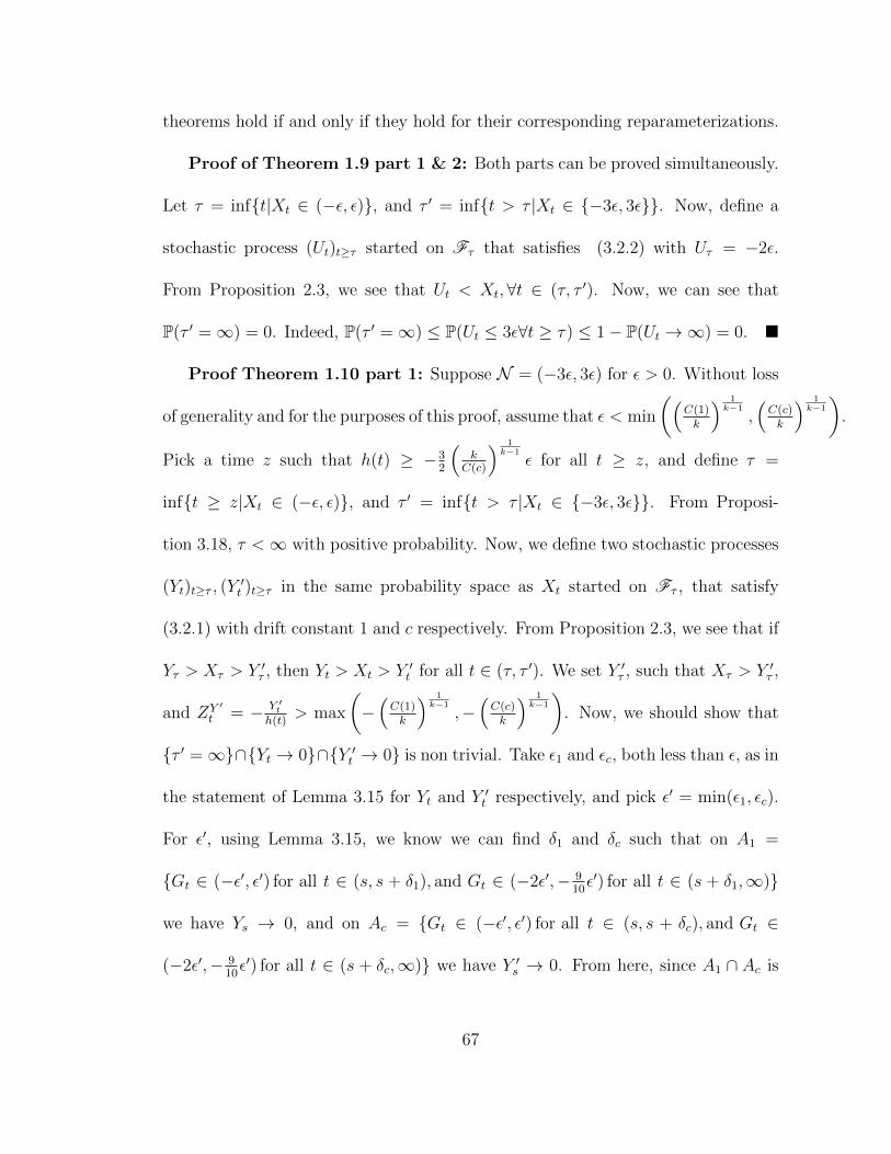
theorems hold if and only if they hold for their corresponding reparameterizations.
Proof of Theorem 1.9 part 1 & 2: Both parts can be proved simultaneously.
Let τ = inft|Xt ∈ (−ε, ε), and τ ′ = inft > τ |Xt ∈ −3ε, 3ε. Now, define a
stochastic process (Ut)t≥τ started on Fτ that satisfies (3.2.2) with Uτ = −2ε.
From Proposition 2.3, we see that Ut < Xt,∀t ∈ (τ, τ ′). Now, we can see that
P(τ ′ =∞) = 0. Indeed, P(τ ′ =∞) ≤ P(Ut ≤ 3ε∀t ≥ τ) ≤ 1− P(Ut →∞) = 0.
Proof Theorem 1.10 part 1: Suppose N = (−3ε, 3ε) for ε > 0. Without loss
of generality and for the purposes of this proof, assume that ε < min
((C(1)k
) 1k−1
,(C(c)k
) 1k−1
).
Pick a time z such that h(t) ≥ −32
(k
C(c)
) 1k−1
ε for all t ≥ z, and define τ =
inft ≥ z|Xt ∈ (−ε, ε), and τ ′ = inft > τ |Xt ∈ −3ε, 3ε. From Proposi-
tion 3.18, τ <∞ with positive probability. Now, we define two stochastic processes
(Yt)t≥τ , (Y′t )t≥τ in the same probability space as Xt started on Fτ , that satisfy
(3.2.1) with drift constant 1 and c respectively. From Proposition 2.3, we see that if
Yτ > Xτ > Y ′τ , then Yt > Xt > Y ′t for all t ∈ (τ, τ ′). We set Y ′τ , such that Xτ > Y ′τ ,
and ZY ′t = − Y ′t
h(t)> max
(−(C(1)k
) 1k−1
,−(C(c)k
) 1k−1
). Now, we should show that
τ ′ =∞∩Yt → 0∩Y ′t → 0 is non trivial. Take ε1 and εc, both less than ε, as in
the statement of Lemma 3.15 for Yt and Y ′t respectively, and pick ε′ = min(ε1, εc).
For ε′, using Lemma 3.15, we know we can find δ1 and δc such that on A1 =
Gt ∈ (−ε′, ε′) for all t ∈ (s, s + δ1), and Gt ∈ (−2ε′,− 910ε′) for all t ∈ (s + δ1,∞)
we have Ys → 0, and on Ac = Gt ∈ (−ε′, ε′) for all t ∈ (s, s + δc), and Gt ∈
(−2ε′,− 910ε′) for all t ∈ (s + δc,∞) we have Y ′s → 0. From here, since A1 ∩ Ac is
67
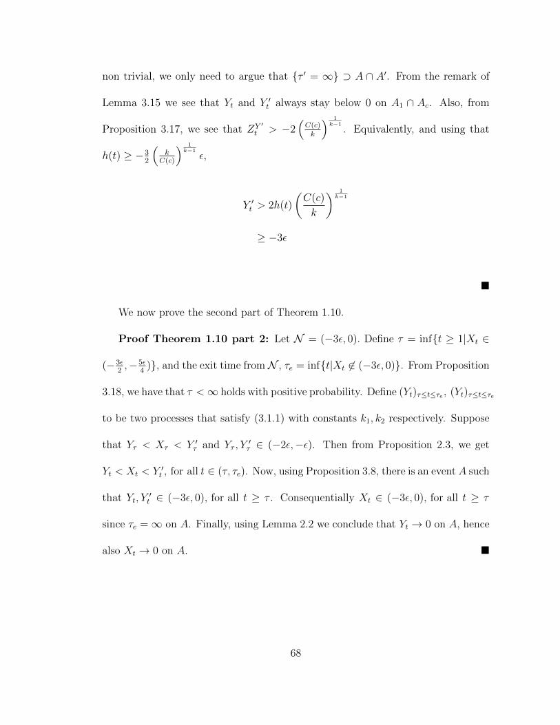
non trivial, we only need to argue that τ ′ = ∞ ⊃ A ∩ A′. From the remark of
Lemma 3.15 we see that Yt and Y ′t always stay below 0 on A1 ∩ Ac. Also, from
Proposition 3.17, we see that ZY ′t > −2
(C(c)k
) 1k−1
. Equivalently, and using that
h(t) ≥ −32
(k
C(c)
) 1k−1
ε,
Y ′t > 2h(t)
(C(c)
k
) 1k−1
≥ −3ε
We now prove the second part of Theorem 1.10.
Proof Theorem 1.10 part 2: Let N = (−3ε, 0). Define τ = inft ≥ 1|Xt ∈
(−3ε2,−5ε
4), and the exit time fromN , τe = inft|Xt 6∈ (−3ε, 0). From Proposition
3.18, we have that τ <∞ holds with positive probability. Define (Yt)τ≤t≤τe , (Yt)τ≤t≤τe
to be two processes that satisfy (3.1.1) with constants k1, k2 respectively. Suppose
that Yτ < Xτ < Y ′τ and Yτ , Y′τ ∈ (−2ε,−ε). Then from Proposition 2.3, we get
Yt < Xt < Y ′t , for all t ∈ (τ, τe). Now, using Proposition 3.8, there is an eventA such
that Yt, Y′t ∈ (−3ε, 0), for all t ≥ τ . Consequentially Xt ∈ (−3ε, 0), for all t ≥ τ
since τe =∞ on A. Finally, using Lemma 2.2 we conclude that Yt → 0 on A, hence
also Xt → 0 on A.
68

Chapter 4
The discrete model
4.1 Analysis of Xn when 12 + 1
2k > γ, k > 1 and
γ ∈ (1/2, 1)
Throughout this section we assume 12
+ 12k> γ. We will prove Theorem 1.11 at the
end of the subsection with the help of Theorem 4.1. The former theorem is a local
version of the latter. For Theorem 4.1 we will need Xn that satisfy
Xn+1 −Xn ≥|Xn|k
nγ+Yn+1
nγ, k > 1 and γ ∈ (1/2, 1), (4.1.1)
where Yn are a.s. bounded and E(Yn+1|Fn) = 0. In this subsection we additionally
require Yn to satisfy E(Y 2n+1|Fn) ≥ l > 0.
Theorem 4.1. Let (Xn)n≥1 solve (4.1.1). Then Xt →∞ a.s..
69

Now, we develop the necessary tools to prove this theorem.
Proposition 4.2. Let (Xn)n≥1 solve (4.1.1). The process (Xn)n≥1 gets close to the
origin infinitely often. More specifically, for β < 0 the event Xn ≥ βn1−2γ
2 i.o. has
probability 1.
Proof: Now, from the restrictions on k we obtain
1
2+
1
2k> γ ⇐⇒ k − 1
2k< 1− γ.
Set h(t) = −t1−γ1−k , and define Zn = −Xn
hn. From here, on the event Xm <
0 for allm ≥ n, we get the following recursion,
Zn+1 − Zn ≥ −Xn+1
h(n+ 1)+
Xn
h(n)(4.1.2)
≥ −Xn
(1
h(n+ 1)− 1
h(n)
)− |Xn|k
nγh(n+ 1)− Yn+1
nγh(n+ 1)
≥ Xn1− γk − 1
ξ− 1−γ
1−k−1n − |Xn|k
nγh(n+ 1)− Yn+1
nγh(n+ 1), where ξn ∈ (n, n+ 1)
≥ Xn
h(n+ 1)nγ
(1− γk − 1
ξ− 1−γ
1−k−1n h(n+ 1)nγ − |Xn|k
Xn
)− Yn+1
nγh(n+ 1)
≥ Xn
h(n+ 1)nγ
(−an
1− γk − 1
|h(n)|k−1 − |Xn|k
Xn
)− Yn+1
nγh(n+ 1)(4.1.3)
≥ Xn
h(n+ 1)nγ
(−2(1− γ)
k − 1|h(n)|k−1 − |Xn|k
Xn
)− Yn+1
nγh(n+ 1)(4.1.4)
where
an =ξ−(1−γ)1−k −1
n h(n+ 1)nγ
−|h(n)|k−1. (4.1.5)
70

To justify the inequality (4.1.4) for large enough n, notice that an → 1.
Define G′s,n =∑n−1
i=sY i+1ih(i+1)
. As seen in 4.1
Lemma 4.3. lim supn→∞G′1,n =∞ a.s..
Proof: We use the following theorem, for a reference see [Fis92] page 676 The-
orem 1,
Theorem 4.4. Let Xn be a martingale difference such that E(X2i |Fi−1) < ∞.
Set s2n =∑n
i=1E(X2i |Fi−1), and define φ(x) = (2 log2(x
2 ∨ e2)) 12 . We assume
that sn → ∞ a.s. and that |Xi| ≤ Kisiφ(si)
a.s. where Ki is Fi−1 measurable with
lim supi→∞Ki < K for some constant K. Then there is a positive constant ε(K)
such that lim supn→∞∑n
i=1Xi
snφ(sn)≥ ε(K) a.s..
It is clear that G′1,n satisfies all the hypothesis required for the aforementioned
theorem to hold.
From Lemma 4.3, it is immediate that for any random time s (not necessarily a
stopping time) lim supn→∞G′s,n =∞, a.s..
Now, we return to prove proposition 4.2. Assume that there is n0 such that
Xn < −(
3(1−γ)k−1
) 1k−1
n1−γ1−k , for all n ≥ n0. Then, since |x|
k
xis increasing we get that
|Xn|kXn
< −3(1−γ)k−1 n−1+γ. Therefore,
−2(1− γ)
k − 1|h(n)|k−1 − |Xn|k
Xn
> −2(1− γ)
k − 1n1−γ +
3(1− γ)
k − 1n1−γ =
(1− γ)
k − 1n−1+γ > 0
71

So,
Zn ≥ Zn0 +n∑
i=n0
Xn
h(n+ 1)nγ
(−2(1− γ)
k − 1|h(n)|k−1 − |Xn|k
Xn
)− Yn+1
nγh(n+ 1)+G′n0,n
> Zn0 +G′n0,n,
which gives lim supn→∞ Zn = ∞ which is a contradiction since this would imply
Xn ≥ 0.
Since n1−γ1−k = o(n
1−2γ2 ), for every constant β < 0, the event Xn ≥ βn
1−2γ2 i.o.,
holds a.s.
We define Gn,u =∑u−1
i=nY i+1iγ
, which is an important quantity for the next lemma
and the remaining of the section.
Lemma 4.5. For any n large enough, we can find a1 > 0, δ > 0 such that P(supu≥nGn,u ≥
a1n1−2γ
2 |Fn) > δ and P(Gn,∞ ≥ a1n1−2γ
2 |Fn) > δ.
Proof: Define τ = infu ≥ n|Gn,u /∈ (−a2n1−2γ
2 , a2n1−2γ
2 ). We calculate the
72

stopped variance of Gτ := Gn,τ . We will do so recursively; fix m ≥ n and calculate,
E((Gτ∧m+1)2|Fn)− E(Gτ∧m)2|Fn) = E
(1τ>m
(2Ym+1
mγGm +
Y 2m+1
m2
)|Fn
)= E
(1τ>m2
Ym+1
mγGm|Fn
)+ E
(1τ>m
Y 2m+1
m2|Fn
)= 0 + E
(1[τ>m]E
(Y 2m+1
m2γ|Fm
)|Fn
)≥ ε
1
m2γE(1[τ>m]|Fn)
≥ ε1
m2γP(τ =∞|Fn).
Therefore,
E((Gτ∧m)2|Fn) ≥ E((Gτ∧n)2|Fn) + cP(τ =∞|Fn)(n1−2γ − (m− 1)1−2γ)
= cP(τ =∞|Fn)(n1−2γ − (m− 1)1−2γ). (4.1.6)
Notice that since Yn are a.s. bounded, |Gτ | ≤ a2n1−2γ
2 + Mnγ
, and since γ > γ − 1/2,
we get that |Gτ | ≤ 2a2n1−2γ
2 for n large enough. For m large, we can find a constant
c′ such that n1−2γ − (m− 1)1−2γ ≥ c′n1−2γ. Using (4.1.6), we obtain
4a22n1−2γ
εc′n1−2γ =4a22εc′≥ P(τ =∞|Fn).
Choosing a2 small enough we may conclude P(τ < ∞|Fn) > 1/2, for all n large
enough.
73

Now, we take any martingale Mn starting at 0, such that it exits an interval
(−2a, 2a), with at least probability p, and |Mn+1 −Mn| < a, a.s.. Then, we stop
the martingale upon exiting the interval (−2a, 2a); namely, define τ− to be the first
time Mn goes below −2a and τ+ to be the first time that Mn surpasses 2a, and set
τ = τ−∧ τ+. Using the optimal stopping theorem for the bounded martingale Mτ∧n
and taking n to infinity we obtain
0 = E(Mτ ) ≤ −2aP(τ− < τ+) + 3aP(τ− > τ+) + 2aP(τ =∞)
= −2ap+ 2a(1− p) + 5aP(τ− > τ+).
So, P(τ− > τ+) ≥ 4p− 2
5, which implies that P(supnMn ≥ 2a) ≥ 4p− 2
5.
The previous applied to Gn,u given Fn, concludes the lemma. Indeed, since
the probability p, of exiting the interval is bigger than 1/2, we may deduce that
4p− 2
5> 0.
For the second part of the lemma, we use the following inequality: let Mn be
a martingale such that M0 = 0 and E(M2n) < ∞. Then P(maxn≥u≥0Mu ≥ λ) ≤
E(M2n)
E(M2n)+λ
2 (for a reference see [Dur13], page 213, exercise 5.4.5). Let τ be the first time
Gn,u, surpasses a2n1−2γ. Condition on [τ < ∞], and notice that Gn,∞ ≥ a2
2n1−2γ
when infu≥τ Gτ,u > −a22n1−2γ. Using the previous inequality, and the fact that x
x+1
74

is increasing gives
P(Gn,∞ ≤a22n
1−2γ2 |Fτ , [τ <∞]) ≤ P(inf
u≥τGτ,u ≤ −
a22n1−2γ|Fτ , [τ <∞])
≤ E((Gτ,∞)2|Fτ , [τ <∞])
E((Gτ,∞)2|Fτ , [τ <∞]) +a224n1−2γ
≤ cτ 1−2γ
cτ 1−2γ +a224n1−2γ
≤ c
c+a224
.
Therefore, P(Gn,∞ ≥ a22n
1−2γ2 |Fn) ≥ P(τ < ∞)
a224
c+a224
, which concludes the lemma.
So, for any stopping time σ, we get the following version of the previous lemma:
Lemma 4.6. For any n, we can find a1 > 0, δ1 > 0, δ2 > 0 such that P(supu≥σ Gσ,u ≥
a1σ1−2γ
2 |Fσ) > δ1 and P(Gσ,∞ ≥ a1σ1−2γ
2 |Fσ) > δ2.
Before proving Theorem 4.1 we will need the following corollary.
Corollary 4.7. Let (Xn)n≥1 solve (4.1.1). The event Xn ≥ 0 i.o. holds a.s.
Proof: For any m,n we get the lower bound Xm − Xn ≥ Gn,m. Now, we
define an increasing sequence of stopping times τn, going to infinity a.s., such that
Xτn ≥ βτ1−2γ
2n for |β| < a1, where a1 is such that the statement of Lemma 4.6 holds.
From Proposition 4.2, we can do so, with all τn a.s. finite. Hence, P(sup∞≥u≥τn Xm−
Xτn ≥ a1τn1−2γ
2 |Fτn) ≥ P(sup∞≥u≥τn Gτn,u ≥ a1τn1−2γ
2 |Fτn) > δ1 > 0. Therefore,
75

by Borel-Cantelli on the events Xτn ≥ βτ1−2γ
2n , we get Xτn ≥ 0 i.o.. Therefore
Xn ≥ 0 i.o. holds a.s.
Proof of Theorem 4.1: Define τn, as in the proof of the previous corollary,
such that Xτn ≥ 0. Since P(Gτn,∞ ≥ a1τ1−2γ
2n |Fτn) > δ2, an application of Borel-
Cantelli shows that Xn ≥ a12n
1−2γ2 i.o. holds a.s.. We claim a.s. there are constants
c(ω) > 0 m(ω) such that Xn > c for all n ≥ m = lim inf→∞Xn > 0. Indeed, if
we define τ0 = 0 and τn+1 = infm > τn + 1|Xm ≥ a12m
1−2γ2 we see that τn < ∞
a.s. and τn →∞. This gives a corresponding filtration, namely Fn = σ(τn).
To finish the claim, we show that A = lim inf→∞Xn ≤ 0 has probability zero.
To do so, it is sufficient to argue that there is a δ such that P(A|Fn) < 1 − δ a.s.
for all n ≥ 1. This is immediate from the previous calculation. Indeed,
P(A|Fn) ≤ 1− P(
lim infn
Xn ≥3a12τ
1−2γ2
n |Fn
)= 1− P
(lim inf
nXn −
a12τ
1−2γ2
n ≥ a1τ1−2γ
2n |Fn
)≤ 1− P(lim inf
nGτn,n ≥ a1τ
1−2γ2
n |Fn)
< 1− δ2.
The process Gm,∞ is a.s. finite, and since the drift term∑
i≥n|Xi|kiγ→ ∞, we get
that Xn →∞.
Finally, we can prove Theorem 1.11. In the next proof Xn, X′n solve (1.8.1) and
(4.1.1), respectively.
76

Proof of Theorem 1.11: We define, τ = infn|Xn ∈ (−ε, ε), and τ ′ = infτ ′ >
τ |Xn 6∈ (−ε′, ε′). When ε is small enough, we may assume that τ <∞ with positive
probability, otherwise we have nothing to prove. On τ <∞, couple Xn with X ′n,
so that P(Xn = X ′n, τ ≤ n ≤ τ ′|[τ < ∞]) = 1, where X ′n is a process that solves
(4.3.1). Since X ′n →∞, a.s., we have that τ ′ <∞ a.s.. Thus, on limn→∞Xn = 0,
Borel-Cantelli implies Xn = 0 i.o.. Therefore, P(limn→∞Xn = 0) = 0.
4.2 Analysis of Xn when 12 + 1
2k < γ, k > 1 and
γ ∈ (1/2, 1)
Before proving the main theorem Theorem 1.12, as described in subsection 1.8 we
will study a process (Xn)n≥1 that satisfies
Xn+1 −Xn ≤f(x)
nγ+Yn+1
nγ, γ ∈ (1/2, 1), k ∈ (1,∞), (4.2.1)
where, f(x) ≤ |x|k when x ∈ (−ε, ε), and f(x) = |x|k when x ∈ R \ (−ε, ε).
Also, as before, |Yn| < M a.s. and E(Yn+1|Fn) = 0. Let x0 < 0, such that
f(x) > M, ∀x ≤ x0. We will use x0 in the next lemma.
Lemma 4.8. Take C = max(M, |X1|, |x0|). Then Xn > −2C for all n a.s..
Proof: We can show this by induction. Of course X1 > −2C. For the inductive
77

step, we distinguish two cases. First, assume that −2C < Xn < −C. Then
Xn+1 = Xn +f(Xn)
nγ+Yn+1
nγ
≥ −2C +f(Xn)
nγ− M
nγ
> −2C.
Now, assume Xn ≥ −C. Then
Xn+1 = Xn +|Xn|k
nγ+Ynnγ
≥ −C + 0− M
nγ
> −2C.
Pick ε > 0 such that ε ≤ min
(14, 12
(1−γ
3(k−1)
) 1k−1
). Let an, be defined as in the
previous subsection 4.1, first appearing in (4.1.3) and defined in (4.1.5).
Claim: Any n0 large enough satisfies the following properties
1. an > 1/2, n ≥ n0.
2. if − Xn+1
h(n+1)> −2ε, and − Xn
h(n)≤ −2ε, then − Xn+1
h(n+1)< −ε, when n ≥ n0.
3. P(G′n0,n ∈ (−ε2, ε2)∀n ≥ n0|Fn0) > 0.
Proof:
78
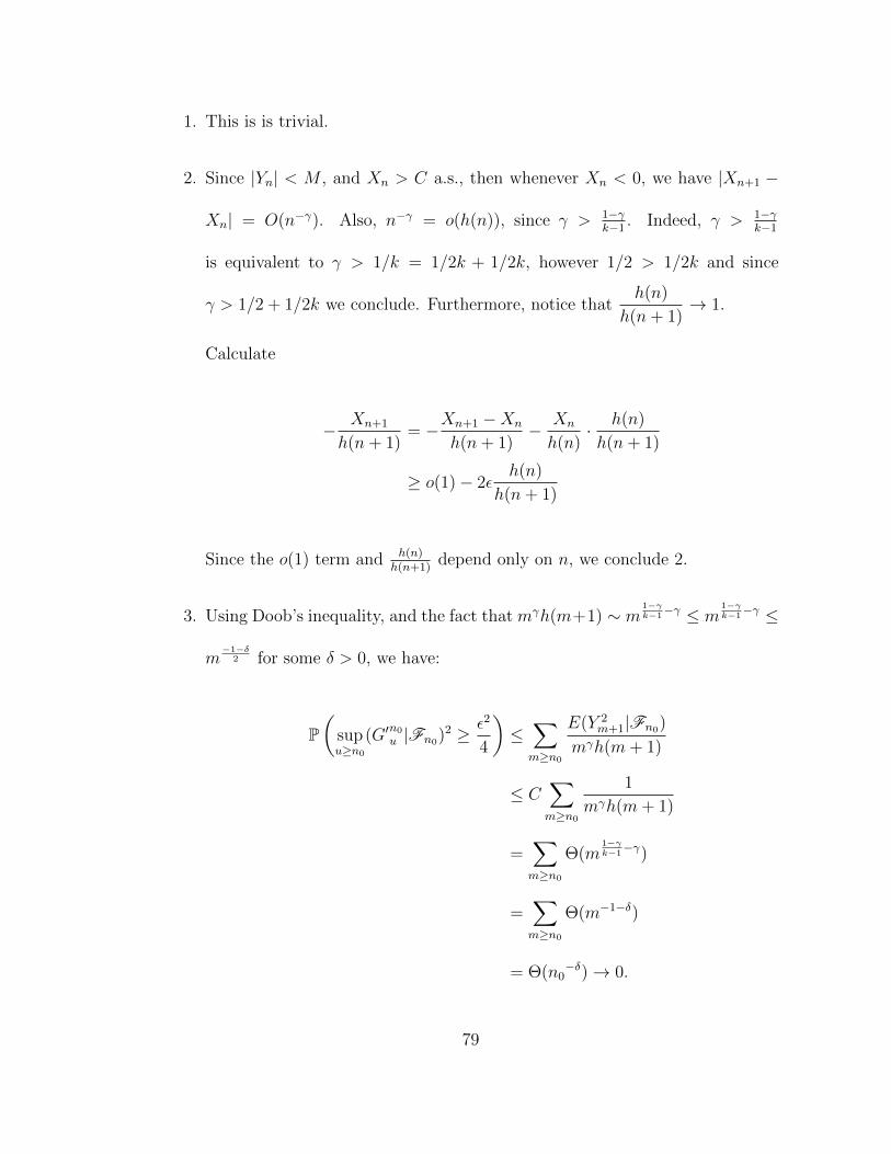
1. This is is trivial.
2. Since |Yn| < M , and Xn > C a.s., then whenever Xn < 0, we have |Xn+1 −
Xn| = O(n−γ). Also, n−γ = o(h(n)), since γ > 1−γk−1 . Indeed, γ > 1−γ
k−1
is equivalent to γ > 1/k = 1/2k + 1/2k, however 1/2 > 1/2k and since
γ > 1/2 + 1/2k we conclude. Furthermore, notice thath(n)
h(n+ 1)→ 1.
Calculate
− Xn+1
h(n+ 1)= −Xn+1 −Xn
h(n+ 1)− Xn
h(n)· h(n)
h(n+ 1)
≥ o(1)− 2εh(n)
h(n+ 1)
Since the o(1) term and h(n)h(n+1)
depend only on n, we conclude 2.
3. Using Doob’s inequality, and the fact that mγh(m+1) ∼ m1−γk−1−γ ≤ m
1−γk−1−γ ≤
m−1−δ
2 for some δ > 0, we have:
P(
supu≥n0
(G′n0
u |Fn0)2 ≥ ε2
4
)≤∑m≥n0
E(Y 2m+1|Fn0)
mγh(m+ 1)
≤ C∑m≥n0
1
mγh(m+ 1)
=∑m≥n0
Θ(m1−γk−1−γ)
=∑m≥n0
Θ(m−1−δ)
= Θ(n0−δ)→ 0.
79

Notice, that the previous claim holds for any stopping time τ , in place of n. So,
we obtain a version of the previous lemma for stopping times.
Lemma 4.9. Let τ be a stopping time such that τ ≥ n0, where n0 is the same as
in the previous claim. Then, P(G′τ,n ∈ (−ε2, ε2)∀n ≥ τ |Fτ ) > 0
Let ε ≤ min
(14, 12
(1−γ
3(k−1)
) 1k−1
), and define a stopping time τ = infn ≥
n0|Zn < −2ε.
Proposition 4.10. Let (Xn)n≥1 that satisfies (4.2.1). When τ <∞, with positive
probability, then P(Xn → 0) > 0. More specifically, the process (Xn : n ≥ τ)
converges to zero with positive probability.
Proof: On the event Xm < 0 for allm ≥ n we use the expression for Zn =
− Xn
h(n)and obtain, as done in (4.1.3), expect, now the inequalities are reversed,
Zn+1 − Zn ≤Xn
h(n+ 1)nγ
(−an
1− γk − 1
|h(n)|k−1 − |Xn|k
Xn
)− Yn+1
nγh(n+ 1)
<Xn
h(n+ 1)nγ
(− 1− γ
2(k − 1)|h(n)|k−1 − |Xn|k
Xn
)− Yn+1
nγh(n+ 1).
Set Dn =Xn
h(n+ 1)nγ
(− 1− γ
2(k − 1)|h(n)|k−1 − |Xn|k
Xn
). Then we have
Zm − Zτ ≤m−1∑i=τ
Di +G′τ,m. (4.2.2)
80
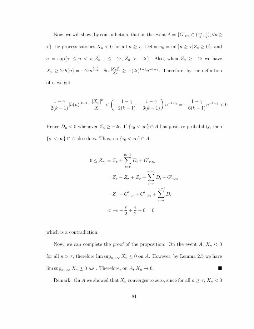
Now, we will show, by contradiction, that on the eventA = G′τ,n ∈ (−ε2, ε2), ∀n ≥
τ the process satisfies Xn < 0 for all n ≥ τ . Define τ0 = infn ≥ τ |Zn ≥ 0, and
σ = supτ ≤ n < τ0|Zn−1 ≤ −2ε, Zn > −2ε. Also, when Zn ≥ −2ε we have
Xn ≥ 2εh(n) = −2εn1−γ1−k . So |Xn|k
Xn≥ −(2ε)k−1n−1+γ. Therefore, by the definition
of ε, we get
− 1− γ2(k − 1)
|h(n)|k−1−|Xn|k
Xn
<
(− 1− γ
2(k − 1)+
1− γ3(k − 1)
)n−1+γ = − 1− γ
6(k − 1)n−1+γ < 0.
Hence Dn < 0 whenever Zn ≥ −2ε. If τ0 <∞ ∩ A has positive probability, then
σ <∞ ∩ A also does. Thus, on τ0 <∞ ∩ A,
0 ≤ Zτ0 = Zτ +
τ0−1∑i=τ
Di +G′τ,τ0
= Zτ − Zσ + Zσ +
τ0−1∑i=τ
Di +G′τ,τ0
= Zσ −G′τ,σ +G′τ,τ0 +
τ0−1∑i=σ
Di
< −ε+ε
2+ε
2+ 0 = 0
which is a contradiction.
Now, we can complete the proof of the proposition. On the event A, Xn < 0
for all n > τ , therefore lim supn→∞Xn ≤ 0 on A. However, by Lemma 2.5 we have
lim supn→∞Xn ≥ 0 a.s.. Therefore, on A, Xn → 0.
Remark: On A we showed that Xn converges to zero, since for all n ≥ τ , Xn < 0
81
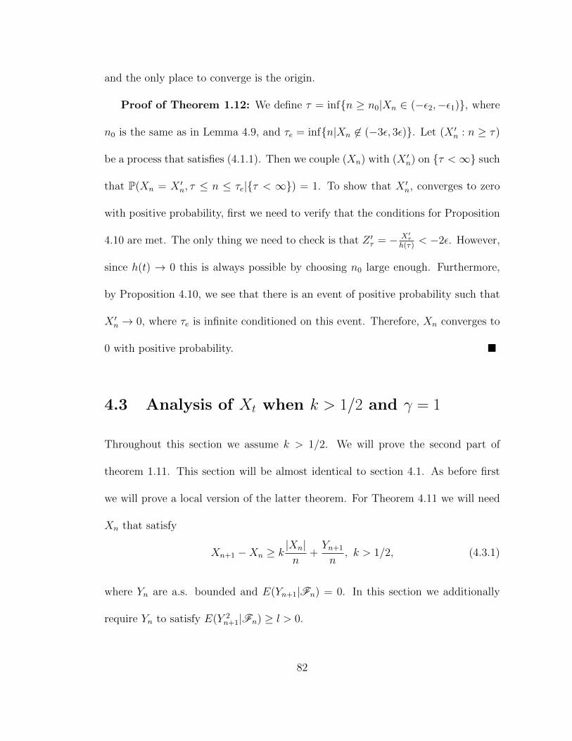
and the only place to converge is the origin.
Proof of Theorem 1.12: We define τ = infn ≥ n0|Xn ∈ (−ε2,−ε1), where
n0 is the same as in Lemma 4.9, and τe = infn|Xn 6∈ (−3ε, 3ε). Let (X ′n : n ≥ τ)
be a process that satisfies (4.1.1). Then we couple (Xn) with (X ′n) on τ <∞ such
that P(Xn = X ′n, τ ≤ n ≤ τe|τ < ∞) = 1. To show that X ′n, converges to zero
with positive probability, first we need to verify that the conditions for Proposition
4.10 are met. The only thing we need to check is that Z ′τ = − X′τh(τ)
< −2ε. However,
since h(t) → 0 this is always possible by choosing n0 large enough. Furthermore,
by Proposition 4.10, we see that there is an event of positive probability such that
X ′n → 0, where τe is infinite conditioned on this event. Therefore, Xn converges to
0 with positive probability.
4.3 Analysis of Xt when k > 1/2 and γ = 1
Throughout this section we assume k > 1/2. We will prove the second part of
theorem 1.11. This section will be almost identical to section 4.1. As before first
we will prove a local version of the latter theorem. For Theorem 4.11 we will need
Xn that satisfy
Xn+1 −Xn ≥ k|Xn|n
+Yn+1
n, k > 1/2, (4.3.1)
where Yn are a.s. bounded and E(Yn+1|Fn) = 0. In this section we additionally
require Yn to satisfy E(Y 2n+1|Fn) ≥ l > 0.
82

Theorem 4.11. Let (Xn)n≥1 solve (4.3.1). Then Xn →∞ a.s..
We have the following proposition corresponding to Proposition 4.2.
Proposition 4.12. Let (Xn)n≥1 solve (4.1.1). The process (Xn)n≥1 gets close to
the origin infinitely often. More specifically, for β < 0 the event Xn ≥ βn−12 i.o.
has probability 1.
Proof: Set h(t) = −t−k, and define Zn = −Xnhn
. Also we pick 1/2 < k1 < k.
From here, on the event Xm < 0 for allm ≥ n, we get the following recursion,
Zn+1 − Zn ≥ −Xn+1
h(n+ 1)+
Xn
h(n)(4.3.2)
≥ −Xn
(1
h(n+ 1)− 1
h(n)
)− k |Xn|
nh(n+ 1)− Yn+1
nh(n+ 1)
≥ Xnkξk−1n − k |Xn|
nh(n+ 1)− Yn+1
nh(n+ 1), where ξn ∈ (n, n+ 1)
≥ Xn
h(n+ 1)n
(kξk−1n h(n+ 1)n− k |Xn|
Xn
)− Yn+1
nh(n+ 1)
≥ Xn
h(n+ 1)n
(−ank − k
|Xn|Xn
)− Yn+1
nh(n+ 1)(4.3.3)
≥ Xn
h(n+ 1)n
(−k1 − k
|Xn|Xn
)− Yn+1
nh(n+ 1)(4.3.4)
≥ Xn
h(n+ 1)n(k − k1)−
Yn+1
nh(n+ 1)(4.3.5)
where
an = −ξk−1n h(n+ 1)n. (4.3.6)
To justify the inequality (4.3.4) for large enough n, notice that an → 1.
83

Define G′s,n =∑n−1
i=sY i+1ih(i+1)
as done in section 4.1 To this end, we have the
following lemma,
Lemma 4.13. lim supn→∞G′1,n =∞ a.s..
Proof: Same proof as Lemma 4.3.
From Lemma 4.13, it is immediate that for any random time s (not necessarily
a stopping time) lim supn→∞G′s,n =∞, a.s..
Now, we return to prove proposition 4.12. Assume that there is n0 such that
Xn < 0, for all n ≥ n0. Then,
Zn ≥ Zn0 +n∑
i=n0
Xi
h(i+ 1)i(k − k1) +G′n0,n
> Zn0 +G′n0,n,
which gives lim supn→∞ Zn = ∞ which is a contradiction since this would imply
Xn ≥ 0.
We define Gn,u =∑u−1
i=nY i+1iγ
. We are almost done since, the noise estimates done
in section 4.1 was a big bulk of the work and they also hold when γ = 1.
Before proving Theorem 4.1 we will need the following corollary.
Corollary 4.14. Let (Xn)n≥1 solve (4.3.1). The event Xn ≥ 0 i.o. holds a.s.
Proof: For any m,n we get the lower bound Xm − Xn ≥ Gn,m. Now, we
define an increasing sequence of stopping times τn, going to infinity a.s., such that
84

Xτn ≥ βτ− 1
2n for |β| < a1, where a1 is such that the statement of Lemma 4.6 holds.
From Proposition 4.2, we can do so, with all τn a.s. finite. Hence, P(sup∞≥u≥τn Xm−
Xτn ≥ a1τn− 1
2 |Fτn) ≥ P(sup∞≥u≥τn Gτn,u ≥ a1τn− 1
2 |Fτn) > δ1 > 0. Therefore, by
Borel-Cantelli on the events Xτn ≥ βτ− 1
2n , we get Xτn ≥ 0 i.o.. Therefore
Xn ≥ 0 i.o. holds a.s.
Proof of Theorem 4.11: Define τn, as in the proof of the previous corollary,
such that Xτn ≥ 0. Since P(Gτn,∞ ≥ a1τ− 1
2n |Fτn) > δ2, an application of Borel-
Cantelli shows that Xn ≥ a12n−
12 i.o. holds a.s.. We claim a.s. there are constants
c(ω) > 0 m(ω) such that Xn > c for all n ≥ m = lim inf→∞Xn > 0. Indeed, if
we define τ0 = 0 and τn+1 = infm > τn + 1|Xm ≥ a12m−
12 we see that τn <∞ a.s.
and τn →∞. This gives a corresponding filtration, namely Fn = σ(τn).
To finish the claim, we show that A = lim inf→∞Xn ≤ 0 has probability zero.
To do so, it is sufficient to argue that there is a δ such that P(A|Fn) < 1 − δ a.s.
for all n ≥ 1. This is immediate from the previous calculation. Indeed,
P(A|Fn) ≤ 1− P(
lim infn
Xn ≥3a12τ− 1
2n |Fn
)= 1− P
(lim inf
nXn −
a12τ− 1
2n ≥ a1τ
− 12
n |Fn
)≤ 1− P(lim inf
nGτn,n ≥ a1τ
− 12
n |Fn)
< 1− δ2.
The process Gm,∞ is a.s. finite, and since the drift term∑
i≥n k|Xi|i→ ∞, we get
85
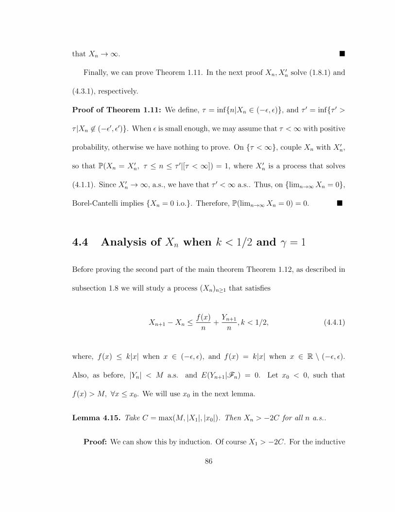
that Xn →∞.
Finally, we can prove Theorem 1.11. In the next proof Xn, X′n solve (1.8.1) and
(4.3.1), respectively.
Proof of Theorem 1.11: We define, τ = infn|Xn ∈ (−ε, ε), and τ ′ = infτ ′ >
τ |Xn 6∈ (−ε′, ε′). When ε is small enough, we may assume that τ <∞ with positive
probability, otherwise we have nothing to prove. On τ <∞, couple Xn with X ′n,
so that P(Xn = X ′n, τ ≤ n ≤ τ ′|[τ < ∞]) = 1, where X ′n is a process that solves
(4.1.1). Since X ′n →∞, a.s., we have that τ ′ <∞ a.s.. Thus, on limn→∞Xn = 0,
Borel-Cantelli implies Xn = 0 i.o.. Therefore, P(limn→∞Xn = 0) = 0.
4.4 Analysis of Xn when k < 1/2 and γ = 1
Before proving the second part of the main theorem Theorem 1.12, as described in
subsection 1.8 we will study a process (Xn)n≥1 that satisfies
Xn+1 −Xn ≤f(x)
n+Yn+1
n, k < 1/2, (4.4.1)
where, f(x) ≤ k|x| when x ∈ (−ε, ε), and f(x) = k|x| when x ∈ R \ (−ε, ε).
Also, as before, |Yn| < M a.s. and E(Yn+1|Fn) = 0. Let x0 < 0, such that
f(x) > M, ∀x ≤ x0. We will use x0 in the next lemma.
Lemma 4.15. Take C = max(M, |X1|, |x0|). Then Xn > −2C for all n a.s..
Proof: We can show this by induction. Of course X1 > −2C. For the inductive
86

step, we distinguish two cases. First, assume that −2C < Xn < −C. Then
Xn+1 = Xn +f(Xn)
n+Yn+1
n
≥ −2C +f(Xn)
n− M
n
> −2C.
Now, assume Xn ≥ −C. Then
Xn+1 = Xn +k|Xn|n
+Ynn
≥ −C + 0− M
n
> −2C.
Let an, be defined as in the previous subsection 4.3, first appearing in (4.3.3)
and defined in (4.3.6).
Claim: Any n0 large enough satisfies the following properties
1. an > 1/2, n ≥ n0.
2. if − Xn+1
h(n+1)> −2ε, and − Xn
h(n)≤ −2ε, then − Xn+1
h(n+1)< −ε, when n ≥ n0.
3. P(G′n0,n ∈ (−ε2, ε2)∀n ≥ n0|Fn0) > 0.
Proof:
87

1. This is is trivial.
2. Since |Yn| < M , and Xn > C a.s., then whenever Xn < 0, we have |Xn+1 −
Xn| = O(n−1) and n−1 = o(h(n)). Furthermore, notice thath(n)
h(n+ 1)→ 1.
Calculate
− Xn+1
h(n+ 1)= −Xn+1 −Xn
h(n+ 1)− Xn
h(n)· h(n)
h(n+ 1)
≥ o(1)− 2εh(n)
h(n+ 1)
Since the o(1) term and h(n)h(n+1)
depend only on n, we conclude 2.
3. Using Doob’s inequality, and the fact that mh(m + 1) ∼ m1−k ≤ m−1−δ
2 for
some δ > 0, we have:
P(
supu≥n0
(G′n0
u |Fn0)2 ≥ ε2
4
)≤∑m≥n0
E(Y 2m+1|Fn0)
m2h2(m+ 1)
≤ C∑m≥n0
1
m2h2(m+ 1)
=∑m≥n0
Θ(m−1−δ)
= Θ(n0−δ)→ 0.
Notice, that the previous claim holds for any stopping time τ , in place of n. So,
we obtain a version of the previous lemma for stopping times.
88
Lemma 4.16. Let τ be a stopping time such that τ ≥ n0, where n0 is the same as
in the previous claim. Then, P(G′τ,n ∈ (−ε2, ε2)∀n ≥ τ |Fτ ) > 0
Let ε > 0, and define a stopping time τ = infn ≥ n0|Zn < −2ε.
Proposition 4.17. Let (Xn)n≥1 that satisfies (4.2.1). When τ <∞, with positive
probability, then P(Xn → 0) > 0. More specifically, the process (Xn : n ≥ τ)
converges to zero with positive probability.
Proof: Pick k2 > k. On the event Xm < 0 for allm ≥ n we use the expression
for Zn = − Xn
h(n)and obtain, as done in (4.3.3), expect, now the inequalities are
reversed,
Zn+1 − Zn ≤Xn
h(n+ 1)n
(−ank − k
|Xn|Xn
)− Yn+1
nh(n+ 1)(4.4.2)
≤ Xn
h(n+ 1)n
(−k2 − k
|Xn|Xn
)− Yn+1
nh(n+ 1)(4.4.3)
≤ Xn
h(n+ 1)n(k − k2)−
Yn+1
nh(n+ 1)(4.4.4)
Set Dn = Xnh(n+1)n
(k − k2). Then we have
Zm − Zτ ≤m−1∑i=τ
Di +G′τ,m. (4.4.5)
Now, we will show, by contradiction, that on the eventA = G′τ,n ∈ (− ε2, ε2),∀n ≥
τ the process satisfies Xn < 0 for all n ≥ τ . Define τ0 = infn ≥ τ |Zn ≥ 0, and
89

σ = supτ ≤ n < τ0|Zn−1 ≤ −2ε, Zn > −2ε. Also Dn < 0 whenever Zn ≥ −2ε.
If τ0 < ∞ ∩ A has positive probability, then σ < ∞ ∩ A also does. Thus, on
τ0 <∞ ∩ A,
0 ≤ Zτ0 = Zτ +
τ0−1∑i=τ
Di +G′τ,τ0
= Zτ − Zσ + Zσ +
τ0−1∑i=τ
Di +G′τ,τ0
= Zσ −G′τ,σ +G′τ,τ0 +
τ0−1∑i=σ
Di
< −ε+ε
2+ε
2+ 0 = 0
which is a contradiction.
Now, we can complete the proof of the proposition. On the event A, Xn < 0
for all n > τ , therefore lim supn→∞Xn ≤ 0 on A. However, by Lemma 2.5 we have
lim supn→∞Xn ≥ 0 a.s.. Therefore, on A, Xn → 0.
Remark: On A we showed that Xn converges to zero, since for all n ≥ τ , Xn < 0
and the only place to converge is the origin.
Proof of Theorem 1.12: We define τ = infn ≥ n0|Xn ∈ (−ε2,−ε1), where
n0 is the same as in Lemma 4.9, and τe = infn|Xn 6∈ (−3ε, 3ε). Let (X ′n : n ≥ τ)
be a process that satisfies (4.1.1). Then we couple (Xn) with (X ′n) on τ <∞ such
that P(Xn = X ′n, τ ≤ n ≤ τe|τ < ∞) = 1. To show that X ′n, converges to zero
with positive probability, first we need to verify that the conditions for Proposition
90

4.17 are met. The only thing we need to check is that Z ′τ = − X′τh(τ)
< −2ε. However,
since h(t) → 0 this is always possible by choosing n0 large enough. Furthermore,
by Proposition 4.17, we see that there is an event of positive probability such that
X ′n → 0, where τe is infinite conditioned on this event. Therefore, Xn converges to
0 with positive probability.
91

Bibliography
[AAZB+17] Naman Agarwal, Zeyuan Allen-Zhu, Brian Bullins, Elad Hazan, and
Tengyu Ma. Finding approximate local minima faster than gradient
descent. In Proceedings of the 49th Annual ACM SIGACT Symposium
on Theory of Computing, STOC 2017, pages 1195–1199, New York,
NY, USA, 2017. ACM.
[AG16] Animashree Anandkumar and Rong Ge. Efficient approaches for es-
caping higher order saddle points in non-convex optimization. In Vi-
taly Feldman, Alexander Rakhlin, and Ohad Shamir, editors, 29th
Annual Conference on Learning Theory, volume 49 of Proceedings of
Machine Learning Research, pages 81–102, Columbia University, New
York, New York, USA, 23–26 Jun 2016. PMLR.
[BR95] Robert W. Brennan and Paul Rogers. Stochastic optimization ap-
plied to a manufacturing system operation problem. In Proceedings of
the 27th Conference on Winter Simulation, WSC ’95, pages 857–864,
Washington, DC, USA, 1995. IEEE Computer Society.
92

[CdlTTZ16] Xi Chen, jason d. lee, Xin T. Tong, and Yichen Zhang. Statistical
inference for model parameters in stochastic gradient descent, 10 2016.
[CHM+15] Anna Choromanska, Mikael Henaff, Michael Mathieu, Grard Ben
Arous, and Yann LeCun. The loss surfaces of multilayer networks.
Journal of Machine Learning Research, 38:192–204, 2015.
[DHS11] John Duchi, Elad Hazan, and Yoram Singer. Adaptive subgradient
methods for online learning and stochastic optimization. J. Mach.
Learn. Res., 12:2121–2159, July 2011.
[DKLH18] Hadi Daneshmand, Jonas Kohler, Aurelien Lucchi, and Thomas Hof-
mann. Escaping saddles with stochastic gradients. In Jennifer Dy
and Andreas Krause, editors, Proceedings of the 35th International
Conference on Machine Learning, volume 80 of Proceedings of Ma-
chine Learning Research, pages 1155–1164, Stockholmsmssan, Stock-
holm Sweden, 10–15 Jul 2018. PMLR.
[Dur13] R. Durrett. Probability: Theory and Examples. Duxbury Press, 2013.
[DZ12] Matthew D. Zeiler. Adadelta: An adaptive learning rate method. 1212,
12 2012.
[EDM04] Eyal Even-Dar and Yishay Mansour. Learning rates for q-learning. J.
Mach. Learn. Res., 5:1–25, December 2004.
93

[EW88] Y.M. Ermoliev and R.J.-B. Wets. Numerical Techniques for Stochastic
Optimization. Springer-Verlag, Heidelberg, 1988.
[Fis92] Evan Fisher. On the law of the iterated logarithm for martingales.
Ann. Probab., 20(2):675–680, 1992.
[GHJY15] Rong Ge, Furong Huang, Chi Jin, and Yang Yuan. Escaping from
saddle points — online stochastic gradient for tensor decomposition.
In Peter Grnwald, Elad Hazan, and Satyen Kale, editors, Proceedings
of The 28th Conference on Learning Theory, volume 40 of Proceedings
of Machine Learning Research, pages 797–842, Paris, France, 03–06
Jul 2015. PMLR.
[GM91] Saul B. Gelfand and Sanjoy K. Mitter. Recursive stochastic algorithms
for global optimization in Rd. SIAM Journal on Control and Optimiza-
tion, 29(5):999–1018, 1991.
[HL13] Christopher J. Hillar and Lek-Heng Lim. Most tensor problems are
np-hard. J. ACM, 60(6):45:1–45:39, November 2013.
[HLS80] Bruce M. Hill, David Lane, and William Sudderth. A strong law for
some generalized urn processes. Ann. Probab., 8(2):214–226, 1980.
[JGN+17] C. Jin, R. Ge, P. Netrapalli, S. M. Kakade, and M. I. Jordan. How to
Escape Saddle Points Efficiently. ArXiv e-prints, March 2017.
94

[JJKN15] Prateek Jain, Chi Jin, Sham M. Kakade, and Praneeth Netrapalli.
Computing matrix squareroot via non convex local search. CoRR,
abs/1507.05854, 2015.
[Kes58] Harry Kesten. Accelerated stochastic approximation. Ann. Math.
Statist., 29(1):41–59, 03 1958.
[KW52] J. Kiefer and J. Wolfowitz. Stochastic estimation of the maximum of a
regression function. The Annals of Mathematical Statistics, 23(3):462–
466, 1952.
[KY03] H. Kushner and G.G. Yin. Stochastic Approximation and Recursive
Algorithms and Applications. Stochastic Modelling and Applied Prob-
ability. Springer New York, 2003.
[LLKC18] Tianyang Li, Liu Liu, Anastasios Kyrillidis, and Constantine Carama-
nis. Statistical inference using sgd, 2018.
[LSJR16] J. D. Lee, M. Simchowitz, M. I. Jordan, and B. Recht. Gradient
Descent Converges to Minimizers. ArXiv e-prints, February 2016.
[NES83] Y. E. NESTEROV. A method for solving the convex programming
problem with convergence rate O(1/k2). Dokl. Akad. Nauk SSSR,
269:543–547, 1983.
95

[Nes00] Yurii Nesterov. Squared Functional Systems and Optimization Prob-
lems, pages 405–440. Springer US, Boston, MA, 2000.
[Pem90] Robin Pemantle. Nonconvergence to unstable points in urn models
and stochastic approximations. Ann. Probab., 18(2):698–712, 1990.
[Pem91] Robin Pemantle. When are touchpoints limits for generalized Polya
urns? Proc. Amer. Math. Soc., 113(1):235–243, 1991.
[Pem07] Robin Pemantle. A survey of random processes with reinforcement.
Probab. Surveys, 4:1–79, 2007.
[PJ92] B. T. Polyak and A. B. Juditsky. Acceleration of stochastic approxi-
mation by averaging. SIAM J. Control Optim., 30(4):838–855, 1992.
[Pol64] Boris Polyak. Some methods of speeding up the convergence of iter-
ation methods. Ussr Computational Mathematics and Mathematical
Physics, 4:1–17, 12 1964.
[RB54] Julius R. Blum. Approximation methods which converge with proba-
bility one. Ann. Math. Statist, 25, 06 1954.
[RM51] Herbert Robbins and Sutton Monro. A stochastic approximation
method. Ann. Math. Statistics, 22:400–407, 1951.
96
[RRT17] M. Raginsky, A. Rakhlin, and M. Telgarsky. Non-convex learning via
Stochastic Gradient Langevin Dynamics: a nonasymptotic analysis.
ArXiv e-prints, February 2017.
[RSS12] Alexander Rakhlin, Ohad Shamir, and Karthik Sridharan. Making
gradient descent optimal for strongly convex stochastic optimization.
In Proceedings of the 29th International Coference on International
Conference on Machine Learning, ICML’12, pages 1571–1578, USA,
2012. Omnipress.
[Rud16] Sebastian Ruder. An overview of gradient descent optimization algo-
rithms. CoRR, abs/1609.04747, 2016.
[Rup88] D. Ruppert. Efficient estimations from a slowly convergent robbins-
monro process. Technical report, Cornell University Operations Re-
search and Industrial Engineering, Cornell University Operations Re-
search and Industrial Engineering, 1988.
[Rup19] David Ruppert. Efficient estimators from a slowly converging robbins-
monro process. 03 2019.
[RWW87] L. C. G. Rogers, D. Williams, and John Wiley. Diffusions, Markov
processes and Martingales, vol 2: Ito calculus. 1987.
[SL87] Rajan Suri and Ying Tat Leung. Single run optimization of a siman
model for closed loop flexible assembly systems. In Proceedings of the
97

19th Conference on Winter Simulation, WSC ’87, pages 738–748, New
York, NY, USA, 1987. ACM.
[SL16] R. Sun and Z. Q. Luo. Guaranteed matrix completion via non-
convex factorization. IEEE Transactions on Information Theory,
62(11):6535–6579, Nov 2016.
[Son12] Pham Tin Son. An explicit bound for the ojasiewicz exponent of real
polynomials. Kodai Math. J., 35(2):311–319, 2012.
[Spr] Springer Verlag GmbH, European Mathematical So-
ciety. Encyclopedia of Mathematics. Website.
URL:https://www.encyclopediaofmath.org/index.php/Lojasiewicz inequality.
Accessed on 2017-10-11.
[SQW17] J. Sun, Q. Qu, and J. Wright. Complete dictionary recovery over the
sphere i: Overview and the geometric picture. IEEE Transactions on
Information Theory, 63(2):853–884, Feb 2017.
[SR96] Sharoni Shafir and Jonathan Roughgarden. Adaptive individuals in
evolving populations. chapter The Effect of Memory Length on Indi-
vidual Fitness in a Lizard, pages 173–186. Addison-Wesley Longman
Publishing Co., Inc., Boston, MA, USA, 1996.
98