Publication No. 04-069-233

CENTRIFUGAL SLURRY PUMP CONCENTRATION LIMIT TESTING AND

EVALUATION -- EXPANSION OF FIPR 04-069-215

FINAL REPORT

Prepared by

GIW INDUSTRIES, INC.

under a grant sponsored by

March 2009

The Florida Institute of Phosphate Research was created in 1978 by the Florida Legislature (Chapter 378.101, Florida Statutes) and empowered to conduct research supportive to the responsible development of the state’s phosphate resources. The Institute has targeted areas of research responsibility. These are: reclamation alternatives in mining and processing, including wetlands reclamation, phosphogypsum storage areas and phosphatic clay containment areas; methods for more efficient, economical and environmentally balanced phosphate recovery and processing; disposal and utilization of phosphatic clay; and environmental effects involving the health and welfare of the people, including those effects related to radiation and water consumption. FIPR is located in Polk County, in the heart of the Central Florida phosphate district. The Institute seeks to serve as an information center on phosphate-related topics and welcomes information requests made in person, or by mail, email, or telephone.

Executive Director Paul R. Clifford

G. Michael Lloyd, Jr.

Director of Research Programs

Research Directors

G. Michael Lloyd, Jr. -Chemical Processing J. Patrick Zhang -Mining & Beneficiation Steven G. Richardson -Reclamation Brian K. Birky -Public & Environmental Health

Publications Editor

Karen J. Stewart

Florida Institute of Phosphate Research 1855 West Main Street Bartow, Florida 33830

(863) 534-7160 Fax: (863) 534-7165

http://www.fipr.state.fl.us

CENTRIFUGAL SLURRY PUMP CONCENTRATION LIMIT TESTING AND EVALUATION - EXPANSION OF FIPR 04-069-215

FINAL REPORT

Graeme R. Addie, VP Engineering and R&D Lee Whitlock, Hydraulic Test Lab Manager

GIW Industries, Inc. Principal Investigators

with

Dr. Anders Sellgren

Luleå University of Technology, Sweden

Prepared for

FLORIDA INSTITUTE OF PHOSPHATE RESEARCH 1855 West Main Street

Bartow, FL 33830

Contract Manager: Patrick Zhang FIPR Contract #04-04-069S

March 2009

DISCLAIMER

The contents of this report are reproduced herein as received from the contractor. The report may have been edited as to format in conformance with the FIPR Style Manual. The opinions, findings and conclusions expressed herein are not necessarily those of the Florida Institute of Phosphate Research, nor does mention of company names or products constitute endorsement by the Florida Institute of Phosphate Research. © 2009, Florida Institute of Phosphate Research.

iii

PERSPECTIVE

Patrick Zhang, Research Director, Beneficiation & Mining

Over 100 million tons of phosphate matrix are transported from mining pits to beneficiation plants in Florida every year. The phosphate matrix is first slurried using high-pressure water guns and then pumped to the beneficiation plants using large-diameter pipelines. Assuming an average slurry density of 35%, the industry needs to pump approximately 300 million tons of matrix slurry annually. In many cases, the mining operations are several miles away from the processing plants. The energy cost for long-distance pumping of such a huge amount of slurry is tremendous. During its peak production years, the Florida phosphate industry consumed about 4 billion KWH of electricity annually, equivalent to $200 million at a price of five cents per KWH. Slurry pumping is believed to account for about one third of the total energy consumption. In general, pipeline friction increases moderately with increasing solids concentrations and particle deposition velocity decreases with increasing mean concentration. Thus, provided there is enough water to make a fluid slurry and the slurry velocity is sufficiently high, higher slurry concentrations lead to higher pipeline transport efficiencies. High concentrations also provide opportunities for reductions in capital cost for equipment. However, centrifugal pumps have upper-limit concentrations beyond which increasing solids becomes less efficient, even without choking the pipeline. Currently very little data are available for the different matrices, tails and consolidated clays at very high concentrations and with large pumps, particularly for the new low NPSH (Net Positive Suction Head) pit pumps. The initial study successfully addressed one of the major problems in a matrix pipeline—that of the variability of the slurry entering the pit pump and the suction lift condition under which the pump operates. In the pit pump operation, a vacuum at the suction inlet is used to draw solids into the pump. The higher the vacuum, the higher the solids concentration ingested. Generally, the higher the concentration in the line, the higher the output and the higher the efficiency of the pipeline. This extension to the initial study rounds out the work of the initial study by providing additional (necessary) matrix models and a way the mine planning personnel can identify which geographical model to use. The extension also provides additional models in the Excel spreadsheet graphical representation format for clay, sand-clay mix, transfer matrix, and tails slurries to provide a one-stop shop for all pipeline pumping needs.

iv

ACKNOWLEDGMENTS

GIW would first like to thank Mosaic and CF Industries for their participation in this project. We would especially like to also thank Pratt Bose, George McQuien, Rick Grove, Glen Oswald, and Greg Long for their input and cooperation in carrying out the field evaluations at Lonesome Mine which was necessary for establishing two of the transport models reported herein. We would also like to thank David Gossett, Bob Klobuchar, Henry Lilly, Amry Tayebi, Chuck Wylie, Damon Lawrence, and Tim Casey for their contributions in regard to the sand-clay mix test program. We are thankful for the model generation by Dr. Kenneth Wilson of Queen’s University, Canada, for the matrix, transfer matrix, and tails models. We also appreciate the contributions of Bob Visintainer in updating the Microsoft Excel model spreadsheets. We would like to express our sincere thanks to Roy Duvall, Scott Yeo, and Jack Condon of the GIW Florida office for their effort with regard to providing field support in arranging the numerous meetings and visits necessary to perform this project. In addition, we are appreciative of the input by Roy relating to the various existing and future slurry transport systems throughout the Florida Phosphate Industry. This project would not have been as successful otherwise. In closing we want to acknowledge the extra effort exhibited by GIW Hydraulic Test Lab staff to ensure this program was completed professionally and in a timely manner. Luís Encarnación and Jonathan Latta contributed to the instrumentation setup, calibrations, and data collection associated with the sand-clay mix test program and field test trailer preparation.

v

ABSTRACT

In the original study, tests were carried out on three different types of phosphate matrix slurries with regards to their pipeline friction, effect on pump head quantity and cavitation performance at (high) concentrations of solids around 40, 50, and 60% by weight. Rheological tests were also carried out as part of FIPR contract No. 04-04-070 (Publication No. 04-069-215) on the fine carrier liquid component of the slurries by the University of Florida. In this extension additional (necessary) matrix, transfer matrix, clay, sand-clay mix, and tails-type slurry models are provided as requested. These are all in the form of one Microsoft Excel spreadsheet for models with graphical output for use by mine planners to cover all phosphate mine pumping needs.

vii

TABLE OF CONTENTS PERSPECTIVE ................................................................................................................. iii ABSTRACT ......................................................................................................................... v ACKNOWLEDGMENTS ................................................................................................. vi EXECUTIVE SUMMARY ................................................................................................. 1 INTRODUCTION ............................................................................................................... 3 GOALS ................................................................................................................................ 5 CHARACTERIZATION OF MATRIX .............................................................................. 7 EXTENSION-STUDY WORK TASKS ........................................................................... 11 FIELD AND LABORATORY TEST WORK .................................................................. 13 Transfer Type Matrix Evaluation........................................................................... 13 Type C Lonesome Matrix Evaluation .................................................................... 15 Type D Wingate Matrix Evaluation ....................................................................... 19 Clay Tests .............................................................................................................. 19 Sand-Clay Laboratory Tests .................................................................................. 20 Tailings Tests ......................................................................................................... 21 HYDRAULIC ANALYSIS AND MODELLING ............................................................. 23 Background ............................................................................................................ 23 Hydraulic Characterization of Matrices ................................................................. 25 B-Type Matrix ........................................................................................... 25 C-Type Matrix ........................................................................................... 26 F-Type Matrix ............................................................................................ 27 Transfer Matrix Slurry ............................................................................... 28 Modelling ............................................................................................................... 29 Matrix Types B, C, and F .......................................................................... 29 Matrix Type D ........................................................................................... 31 Tailings ...................................................................................................... 31 Clay ............................................................................................................ 31 Sand-Clay ................................................................................................... 32 Variability Coefficient ............................................................................... 33 Effect of Solids on Head and Efficiency ............................................................... 33

viii

TABLE OF CONTENTS (CONT.) USE OF THE EXCEL SPREADSHEET .......................................................................... 35 General Notes for Using the Excel Spreadsheet .................................................... 36 Spreadsheet Protection ........................................................................................... 36 EXCEL SPREADSHEET RESULTS AND GRAPHICAL OUTPUT ............................. 39 DISCUSSION .................................................................................................................... 43 Pipeline Pumping ................................................................................................... 43 Pit Operation .......................................................................................................... 43 Flow Mechanisms .................................................................................................. 44 SUMMARY OBSERVATIONS ....................................................................................... 47 CONCLUSIONS ............................................................................................................... 49 REFERENCES .................................................................................................................. 51 APPENDICES (ON ENCLOSED CD) A. Transfer Type Matrix Evaluation Data and Slysel Analysis Sheets ............. A-1 B. Type C Matrix Train 18 Lonesome Data and Slysel Analysis Sheets ........... B-1 C. Type C Train 18 Lonesome Solids Size Analysis Test .................................. C-1 D. Sand-Clay Mix Lab Tests ............................................................................. D-1 E. Clay-Only Lab Test Data ............................................................................... E-1 F. Modelling Pipeline Flow of Non-Newtonian Slurries (Paper) ....................... F-1 G. Validation of a Four-Component Pipeline Friction Loss Model (Paper) ..... G-1 H. Microsoft Excel Spreadsheet Model Output for All Types of Slurries ........ H-1 I. PCS Matrix Transportation Optimization (Presentation) ................................. I-1 J. Type D Matrix Wingate Pumping Evaluation .................................................. J-1

ix

LIST OF FIGURES

Figure Page

1. Central Florida Phosphate Area Mine Locations ..................................................... 9 2. Triangular Coordinate Matrix Sizing ..................................................................... 10 3. The Field Test of the Train 18 Pipeline and Transfer Matrix System ................... 16 4. Hydraulic Gradient j Versus Velocity for Cw=60%, D =21” ................................ 17 5. Hydraulic Gradient j Versus Velocity for Cw = 35 and 50%, D = 21” ................. 18 6. Pipe Wall Shear Stress in psf Versus the Scaling Parameter 8V/D, D=3” ............ 20 7. Wall Shear Stress Versus 8V/D for Sand-Clay Slurry .......................................... 21 8. Friction Loss Gradient j in Feet of Slurry per Foot of Pipe for Type B ................ 25 9. Friction Losses for the C Matrix Based on the Evaluations in Figures 4 & 5 ....... 26 10. Friction Loss Gradient for F Matrix in Table 8 ..................................................... 27 11. Friction Loss Gradient for a Pretreated Transfer Matrix Slurry ............................ 28 12. Schematic Description of Clay Friction Loss Modelling ...................................... 32 13. Sketch Defining the Reduction in Head and Efficiency of a Pump ....................... 33 14. Head Loss Versus Velocity Plot ............................................................................ 39 15. Energy Versus Production Plot with Cw and Velocity .......................................... 40 16. Energy Versus Production with Cw and Gun Water ............................................. 40 17. Friction Losses for Cw from 40 to 64% (Sand 3) .................................................. 44 18. Estimated Span of Particle Size Distribution for Pumped Matrix Ore .................. 45 19. Schematic Illustration of the Matrix Slurry Friction Losses .................................. 46

xi

LIST OF TABLES Table Page 1. List of Matrix Mines, Solids Size, and Type ........................................................... 8 2. List of Mosaic Transfer Pipeline Pumps ................................................................ 14 3. Lonesome Transfer Matrix Filtered Field Data, D = 21” ...................................... 15 4. Type C Matrix Lonesome Train 18 Pumps ........................................................... 15 5. Lonesome Mine Train 18 Pipeline Lengths ........................................................... 16 6. Background Laboratory and Field Data for Type B .............................................. 25 7. Background Field Data for Type C Matrix ............................................................ 26 8. Background Laboratory and Field Data for Type F Matrix ................................... 27 9. Background Field Data for Transfer Type Matrix ................................................. 28 10. Summary of Average Friction Losses in Feet of Slurry per Foot of Pipe ............. 29 11. Empirically Determined Values of B and p in Equation 5 .................................... 31 12. Evaluation of Increased Capacity Effects on Water and Energy Savings ............. 43

1

EXECUTIVE SUMMARY

This extension complements the work of an earlier study, Publication No. 04-069-215, designed to categorize phosphate matrix, to put its pipeline pumping characteristics into an Excel format with an easy-to-use graphical output and utilize those to achieve energy cost savings. It also provides additional models in the same format for transfer matrix, clay, sand-clay mix, and tails slurries requested by the mine personnel. The original work, while successful in itself, did not cover all types of matrix now being pumped and it did not provide a clear way for mine planners to identify geographically what model to use. This extension provides the additional models necessary to cover all types of matrix and a guide on when to use them. The extra models for transfer matrix, clay, sand-clay mix, and tails are now included so that all of the mine planners’ phosphate solids, pipeline transport, pipe friction, and energy assessment needs are in one easy-to-use tool. The main purpose was to categorize the pipeline friction and energy needs of all types of matrix along with methodology of when (geographically) to use those in an easy-to-use Excel spreadsheet format. It was also a goal to provide similar models for transfer matrix, clays, sand-clay mix, and tails phosphate slurries in the same common Excel format, complete with easy-to-interpret geographical output. The field and laboratory results up to February 2007 have formed the background for the hydraulic analysis. Furthermore, available large-scale loop test and field measurement results with matrix ore slurries from the first FIPR study in 1988 have been re-analyzed and used as background data for the modelling of slurry friction losses. The modelling of typical clay-only slurries has been based on loop test results for various diameters while the detailed sand-clay model was based on small modifications of the clay model based on experimental results. Finally the tails model mainly goes back to sand data obtained over the years at the GIW Hydraulic Laboratory. The specific energy consumption to overcome pipeline friction losses for the central Florida Type B and Type C matrices at 60w% was about 0.34 and 0.31 hp-hr/ton-mile, respectively, when pumped at 16 fps in a 21” pipeline. The corresponding energy requirement for Northern Florida Type F at the same conditions was 0.38 hp-hr/ton-mile. The field evaluations of the pump performance in matrix slurry pumping indicated together with earlier full-scale laboratory results that the overall reduction in efficiency, including the influence of successive wear increases in proportion to the solids concentration, to be about 10% at 60w%.

2

The favorable pumping conditions in the field for the B- and C-type matrices may be related to a seemingly well balanced particle size distribution with pebbles and fines content of about 25% and 15%, respectively. Tests, analysis, and spreadsheet development were carried out for the different types of matrices, a transfer matrix, a tails, a clay-sand mix, and a clay-only type of phosphate slurries. Excel spreadsheets and models with graphical output were developed for all of these and made available in this report. A way of selecting the different matrix models and other types of slurries has been provided such that a mine planner can use these for a variety of different pipeline diameters, concentrations, and other cases. As laid out, it is hoped the spreadsheet will cover all the phosphate mine planner’s pumping pipeline friction needs. All of the model plots provide the ability to evaluate energy consumption for different scenarios. The matrix models include special plots that show how gun water needs to be controlled to reduce pumping costs. These models and plots indicate significant savings could be achieved by operating at the most efficient point for a particular slurry. The evaluation data collected supports that operating this way is indeed possible from a pumping viewpoint.

3

INTRODUCTION Over 100 million tons of phosphate matrices are transported from mining pits to beneficiation plants in Florida every year. The phosphate matrix is first removed from the ground using drag lines then slurried in a hole (pit) in the ground using high-pressure water guns and then pumped to the beneficiation plants using large pumps pumping into large diameter pipelines. The electrical operating cost, the wear parts, and capital (interest) cost for the pump portion of a typical eleven pump matrix train transporting 1500 TPH of dry solids at a concentration by weight of 30% by weight is in excess of 5 million dollars per year. There are approximately 17 matrix trains in operation in Florida throughout the industry. Pipeline lengths are expected to grow, thus increasing this cost. Studies are able to show that if the solids concentration is increased to 50% by weight without increasing pipeline velocities, then pumping costs can be reduced by 40% or more. This could result in savings to the industry of $50 million or more a year. Consistent higher concentration operation has not been possible in the past because of limitations at the pit and lack of knowledge on how and when higher concentrations may be used. The pit (pump) limitation has been, to a large extent, eliminated by larger, slower-running special pit pumps. The pipeline pumping knowledge and control techniques necessary to take advantage of this have not yet been established. Work has been done in the past to categorize Florida Phosphate matrix as to its pipeline performance and how it may be more cost effectively transported from the mine (pit) to the wash plant. Tests in 1989 (Publication No. 04-037-078) were carried out on difficult (Noralyn mine), easy (Suwannee mine), and average (Hookers Prairie mine) types of matrix. The later high-concentration (Publication No. 04-069-215) 2005 test was carried out on matrix from PCS Swift Creek, IMC Kingsford, and Cargill South Fort Meade. While the above tests provided a wide variety of data on matrix it turned out that the criteria for energy-effectiveness were different and site-specific. Some of the mines where the data came from have also shut down and it is not clear to the mine planning people when the data from the types tested could be used at other mines or geographical locations. In preparation for this proposal, a study of all of the matrix mines in Florida was carried out. This indicated that they could be geologically broken down and identified as being of one of six different types for the purposes of pipeline performance evaluation.

4

A further review shows the data collected previously could cover four of the above six, but that additional data and analysis were needed for the remaining two, including the pre-washer (transfer matrix) type. A part of the 2004 study (Publication No. 04-069-215) was the establishment of a Microsoft Excel spreadsheet model with easy-to-use graphs for determination of pipe friction, minimum energy and gun water. While matrix pumping forms the largest part of the pumping, there is also a need for a spreadsheet-format, easy-to-use graphical pumping guide for tails, transfer matrix (noted earlier), clay and sand-clay mix type of phosphate slurries. This portion of the work extends the spreadsheet to cover the remaining slurry types. Lab tests had to be carried out for the sand-clay mix types, extra field tests for the missing matrix types, and existing data was used for the tails and clay-only types to create the additional spreadsheets. In its completed form, this study provides the mine planning personnel with one tool to cover all pipeline performance and energy needs. This was the main goal of this study extension and report.

5

GOALS

To categorize the pipeline friction and energy needs of all known types of matrix along with a methodology of when (geographically) to use those in an easy-to-use Excel spreadsheet format. To provide similar models for transfer matrix, clays, sand-clay mix, and tails phosphate slurries in the same common Excel format, complete with easy-to-interpret graphical output.

7

CHARACTERIZATION OF MATRIX

As higher-grade deposits have been depleted, the mining of matrix has moved south in the Central Florida Phosphate district into lower-grade deposits. The deposits currently being mined are mainly composed of clay and quartz sand, with widely varying amounts of sand-sized phosphate (Scott and Courtney 2006). In northern Florida there is one deposit actively mined at present. The geological background and local variability has a strong influence on the pumping characteristics. It is necessary for mine planning people to know the geological characteristics of the matrix slurry and what its pumping characteristics will be in the setting up of the pumping equipment. A dragline digs out the phosphate matrix (ore) and dumps it into a pit. The dragline operators are often able to avoid the poorest ore spots or dump some clay-sand buckets at the side. The ore is then successively pushed into the pit with the bucket which gives some mixing before the matrix is slurried using a high-pressure water gun. In the pit the matrix passes through 6”-wide bars and the flow is picked up by the pit pump, which is located slightly above the pit water level. Thereafter the slurry is pumped, typically in a 19” ID-pipeline, with booster pumps distributed along the line to the wash or processing plant. The described “beneficiation” or screening in the handling of the raw ore up to the pit pumping may result in a transported product with a smaller content of fines than indicated by the geological survey data. For example, in one area (Area F), overall averaged values from 590 boreholes showed that the pebble-to-fines %-content ratio was 2.4/24. Matrix pumping testing from that area indicated a maximum fines content of about 13%. Similar comparisons at other locations for various field and laboratory tests indicate that the fines content, as an average, is about half the maximum values observed in boreholes. There is an infinite variation in the solids size and solids distribution of the slurries pumped. In reality, a finite number of types may be established that for all practical purposes could cover the range encountered. As a result of discussions between the geological personnel and the GIW investigators, six types have been chosen to represent all matrix types for the purpose of pipeline calculations and planning. These, along with a description of the associated matrix type, are shown in Table 1, and the mines they are purported to represent are shown in Figure 1. It should be noted that the Type E (Noralyn) mine has closed permanently and the Type D mine (Wingate) has recently started up again.

8

Table 1. List of Matrix Mines, Solids Size, and Type.

No. Mine % Pebble

% Fines

Friction Matrix Type Suggested Comments

1 Four Corners 6.2 37.0 A

2 Hookers Prairie 14.0 24.0 B Ref.: 1989 Publication No. 04-037-078

3 South Fort Meade 13.3 34.1 B Ref.: 2005 Publication No. 04-069-215

4 Kingsford 17.5 25.0 B Ref.: 2005 Publication No. 04-069-215

5 Hopewell 13.8 33.9 B 6 Fort Green 6.6 27.4 C* 7 Lonesome 8.5 29.4 C* 8 Pine Level 6.5 20.5 C* New Mine 9 Ona 6.1 33.2 C* New Mine 10 Pioneer 4.5 30.8 C* New Mine 11 Keys 6.5 26.1 C* 12 Hardee County 6.8 29.4 C* 13 Wingate Creek 5.7 16.4 D*

14 Noralyn 46.0 28.0 E Ref.: 1989 Publication No. 04-037-078

15 Suwannee River-White Springs 1.0 12.0 F Ref.: 1989 Publication No. 04-037-

078

16 Swift Creek-White Springs 2.0 13.0 F Ref.: 2005 Publication No. 04-069-

215

9

Figure 1. Central Florida Phosphate Area Mining Locations (see Table 1).

10

As a result of the segregation at the pit (noted earlier), experience has shown that Type A can, for all intents and purposes, be regarded as being equivalent to the Type B matrix. The new transfer type of preprocessed matrix and Type C, as noted in the extension proposal, were categorized by studies at the Lonesome mine (Train 18) pipeline. The solids size of the different matrix slurries is shown in respect of fines, pebble, and feed in Figure 2 below using the industry common method where fines are % by weight < 100 micron, and pebble is % by weight > 1000 micron. The inset figure denotes the pumpability.

Figure 2. Triangular Coordinate Matrix Sizing.

11

EXTENSION-STUDY WORK TASKS As noted earlier, categorization of tails, sand-clay mix, transfer type matrix, and the Type C matrix are included in this extension and are to be combined with data collected in the original study. Microsoft Excel models have been created for all of these; they are set up in the one-stop-shop pipeline evaluation spreadsheet. As noted earlier, the tailings model was developed using data collected earlier. A separate section on the tailings model follows in this report. The sand-clay mix slurry is a special mix of clay and tailings in different defined proportions. The basis of the sand-clay model(s) is GIW test data and tests carried out in the GIW lab on samples provided by CF Industries. The results of these tests and the evaluation are reported later in this document. The clay-only model is based on tests carried out at GIW and again is reported separately later in this document. Matrix Types A, B, and F have already been reported (Publication No. 04-037-078) as part of the process of looking at the complete pumping picture. Matrix Types B and F (reported earlier) have been reviewed and adjusted as necessary based on the latest tests. They, along with the models and spreadsheet pages, are included later in this report. Field tests were carried out on C matrix and transfer matrix as part of this extension. The Mosaic mine production schedule was such that the installation of the GIW ‘U’ loop density meter could not be installed before early 2007; therefore, initial data was collected using an evaluation of the matrix slurry. In February of 2007, Mosaic enabled GIW to perform a field test at the pit of Train 18, Lonesome Mine, enabling data collection up to higher concentrations without pump cavitation. The results presented here are based on both the evaluation and the February field test.

13

FIELD AND LABORATORY TEST WORK

TRANSFER TYPE MATRIX EVALUATION As noted earlier, the production situation at Mosaic initially would not allow a stoppage for installation of the GIW inverted U-loop density meter and magnetic flow meter. An evaluation of transfer system matrix slurry was therefore carried out as an alternative method of determining the pipeline friction characteristics. In a normal pipe friction test, the head loss over a length of horizontal pipe is measured at a given flow and concentration. The head loss per foot of pipe is then calculated at various solids concentrations and velocities and evaluated against different models. In a lab, the distance (for reasons of practicality) may be only 50 feet and the slurry is recirculated in a closed loop. Good accuracy is generally achieved here, the main disadvantage being the possibility of degradation of the slurry and the sample being in some way biased. In the field, the same test may be carried out over a longer horizontal run, correcting for the less accurate readings. Here the slurry is more real in the sense that it is actually what is going down the pipeline. The main disadvantage of the field test is that production determines what happens and the range of concentrations and velocities is likely to be more restricted than it is in a lab test. In this case, the patented GIW inverted U-loop is usually used with a magnetic flow meter to get density and pipeline velocity. The instrumentation and operation data now available in the mines is quite good compared to 10-15 years ago. Data is now monitored, stored, and maintained where it can be made available as needed. In this case, pipeline flow rate, mean density, and drive train ampere readings from all of the operating pump units were available. The pumps employed in the pipeline can be hydraulically identified along with the driver details. Tested water performances are available for most of these pumps. Derates for slurry solids effect can be applied and component wear accounted for. Subsequently, if we have the pump speed, we can calculate the head produced by each pump. If the head produced by each pump in the line is summed and any known static head (Hs) subtracted (usually about 80 feet), then the pipe friction for a given mean concentration and velocity can be determined using the simple relation:

))ft(lengthpipeline

Hsheadpump()pipeofft/mixtureft(frictionPipe ∑ −

=

14

This, of course, is for a given moment or period in time, at a given operating flow, a given solids concentration, and given (maximum) motor speed(s). Where the motor speed is variable (and/or unknown) the motor amps can be used to estimate the speed. Motor output power (P) is calculated using the relations:

P=v3 EI cos f where E (volts) is normally 4160, cos f is power factor (normally 0.8) and

?3960SGHQ

P×××

=

where Q is flow in GPM, H is TDH in feet of mixture, SG is relative density of mixture, ? is pump and drive train combined efficiency. Here the efficiency, ?, needs to include the effect of the solids, the drive train efficiency (motor and gearbox), and an allowance for any wear or maladjustment. The Mosaic data collected over time and provided to the investigators in Excel format can be sorted and filtered to identify flow, concentration, and amp readings that can be used as data for a model. In the case of the transfer type matrix system, the pumps employed are as shown in Table 2 (below) along with the equivalent GIW assembly, impeller diameter, power, max RPM, and duty speed used in the November 15th calibration tests. Table 2. List of Mosaic Transfer Pipeline Pumps.

Pump Assembly

Slysel No.

Mosaic No.

Pump Type

Impeller Diameter (in) Motor hp/rpm

RPMon 11/15

5252C 1 CSS WBC 54 53" 2000/5105252C 2 10 UBD 54 52" 2000/500 DC 3485252C 3 9 UBD 54 52" 2000/5106135D 4 8 TBD 54 52" 2000/510 VF 2466135D 5 7 TBC 54 52" 2000/5106135D 6 6 TBC 54 52" 2000/5106135D 7 5 TBC 54 52" 2000/510 VF 257Z0001 8 4 T 52 48" 1600/505Z0001 9 3 TBC 54 52" 2000/510Z0001 10 2 TBC 54 52" 2000/510 Z0001 11 1 TBC 54 52" 2000/510 VF 514

At a mean flow rate value of 19,000 gpm during the November 15th calibration runs over a 53,888 foot long pipeline, the solids concentration averaged 30% by weight.

15

During the time period of the test, the calculated total pump head less the 100 feet of static resulted in a hydraulic gradient of 0.0339 feet of mixture per foot of pipe. The Slysel program summary and Microsoft Excel spreadsheet are provided in Appendices A and H, respectively. By filtering data provided by Mosaic it was possible to establish gradient values for different concentrations as shown in Table 3. Full Slysel program output sheets and filtered data are provided in Appendix A. Table 3. Lonesome Transfer Matrix Filtered Field Data, D = 21”.

Cw (%) Flow Rate (GPM) j (ft/ft) 30 19000 0.0339 30 20621 0.0367 25 18902 0.0339 20 19255 0.0340

TYPE C LONESOME MATRIX EVALUATION The Type C Train 18 Lonesome matrix system was evaluated in a similar way to that described in the Transfer Matrix section. In this case, the pumps employed were as shown in Table 4. Table 4. Type C Matrix Lonesome Train 18 Pumps.

Assembly Slysel No. Mosaic No. Pump Type Imp Dia Motor Hp/rpm

6223C 1 LSA 62 62” 1500 / 325 9220D 2 4 WBC 50 49” 1600 /505 8334D 3 3 WBC 46 45” 1500 / 505 7450D 4 2 WBC 54 48” 1500 / 510 2260D 5 1 WBC 48 48” 1600 / 505

During the calibration runs on November 15th, all pumps were operated at maximum speed at an average concentration of 35% at approximately 16,880 gpm against a pipeline configuration as shown in Table 5.

16

Table 5. Lonesome Mine Train 18 Pipeline Lengths. The static head was 86.1 feet, resulting in a net hydraulic gradient of 0.0434 feet of mixture per foot of pipe (not adjusted to account for the varying pipe diameters).

Figure 3. Field Test of the Train 18 Pipeline and Transfer Matrix System. Figure 3 shows the field test unit as set up for data collection on February 14-15, 2007. Operating data collected during the field test were evaluated in terms of friction loss gradients versus velocities. Results for three solids concentrations based on a sorting and filtering spreadsheet procedure are presented in Figures 4 and 5 together with a modelling approach (dashed line).

Conduit Pipe ID (inch) Pipe Length (ft) Suction 23.2 25

Disch. #1 21.0 693 Disch. #2 21.0 668 Disch. #3 19.0 1453 Disch. #4 19.0 4752 Disch. #5 19.0 4858 Disch. #6 19.0 3802

Total Line Length: 16251

17

Summary of data averages for velocity versus hydraulic gradient, J

0

0.01

0.02

0.03

0.04

0.05

0.06

0.07

0 2 4 6 8 10 12 14 16 18

Velocity (ft/sec)

Hyd

rau

lic G

rad

ien

t, J

(ft

/ft)

60w%, 13 ft/sec 60w%, 14 ft/sec 60w%, 15 ft/sec Water Modeling Approach

Figure 4. Hydraulic Gradient j Versus Velocity for Cw=60% D, = 21”. The dashed model approach in Figure 4 may conservatively estimate the friction loss gradient to about 0.035 feet of slurry per foot of pipe for 16 fps. The fluctuations seen in Figure 4 as observed in the 100 foot long test section are typical for dredge-like systems. Based on the results in Figure 4, friction losses in the whole system for lower solids concentrations should not exceed the values in Figure 4 for the considered velocities, following accepted theories and experiences. However, it was observed that the degree of fluctuations was larger at lower solids concentrations and velocities (see Figure 5).

18

Summary of data averages for velocity versus hydraulic gradient, J

0

0.01

0.02

0.03

0.04

0.05

0.06

0.07

0 2 4 6 8 10 12 14 16 18

Velocity (ft/sec)

Hyd

rau

lic G

rad

ien

t, J

(ft

/ft)

35w%, 13 ft/sec 35w%, 14 ft/sec Water Modeling Approach

Summary of data averages for velocity versus hydraulic gradient, J

0

0.01

0.02

0.03

0.04

0.05

0.06

0.07

0 2 4 6 8 10 12 14 16 18

Velocity (ft/sec)

Hyd

rau

lic G

rad

ien

t, J

(ft/

ft)

50w%, 13 ft/sec 50w%, 14 ft/sec 50w%, 15 ft/sec Water Modeling Approach

Figure 5. Hydraulic Gradient j Versus Velocity for Cw= 35 and 50%, D = 21”. In a matrix pipeline system operating with a low average velocity of Cw about 35%, more particles are transported close to the bottom of the pipe than for a Cw of about 60%. The associated variations in the local particle velocities contribute to density fluctuations in the flow generated from the pit. For modelling in this study, only average operating velocities in excess of 14 fps will be considered. Realistic operating friction loss conditions have been represented by the dashed line in Figures 4 and 5, which serve as the basis for the modelling. Subsequently, the considered gradient is approximately independent of the solids

19

concentration and corresponds to favorable operating conditions close to the corresponding water curve. However, the system must be designed to cope with the inherent sudden fluctuations. Slurry samples collected in the pit indicated that about 15% of the particles were smaller than 100 micron, with 25% being larger than 1000 micron, i.e., rather broad gradings. TYPE D WINGATE MATRIX EVALUATION The Type D matrix (Wingate) is similar to Type F except that it has 3-4% higher pebble and fines contents. As a check, a field evaluation was carried out by Roy Duvall and the results are provided in Appendix J. CLAY TESTS

Florida phosphate clays (from a variety of locations) have been tested and analyzed many times over the years in multiple test loop systems at the GIW Hydraulic Lab. Though referred to as pure clays, this slurry in fact contains a small proportion of up to 100 micron sand solids. Full scale tests were carried out in 1991 for the Cargill Company in the 19¼” diameter pipe loop. Furthermore, every year a sample is tested at the annual GIW Slurry Course. Dr. M. R. Carstens, one of GIW’s former consultants, has written reports which form the basis for the GIW Slysel clay model. Recent tests have been performed in the 3” loop allowing GIW to gather data up to a slurry SG of 1.20, which is well beyond field capabilities. Examples of various results are shown in Figure 6, which forms the basis for model development. This figure presents data in the familiar form of scaling parameter (8V/D) versus pipe wall shear stress (t 0). V is velocity and D is pipeline inner diameter.

20

Figure 6. Pipe Wall Shear Stress in psf Versus the Scaling Parameter 8V/D, D = 3”. From Figure 6, it is apparent how sensitive the friction resistance is in relation to the slurry SG. Values of 1.10 and 1.20 correspond to solids concentrations by weight of 16 and 26%, respectively. The wall shear stress at 8V/D=100, for example, is about 5 times larger for 26 than for 16%. The primary data used to create the clay model are shown in Appendix E. SAND-CLAY LABORATORY TESTS The sand-clay mix type of slurry represents a special type which is currently applied at CF Industries. Sand-clay consists of combining a stream of phosphate clay from an impoundment area with a stream of semi-dry sand tailings to form a mixture that is believed to dewater more quickly than clay alone. The clays are provided from the bottom of an impoundment area using a floating dredge. The sand is provided separately and mixed in a special tank which is then pumped away to the reclamation area in a 19” pipeline. Illustrative diagrams of this process have been provided in Appendix D for combining clay SGs from 1.08-1.14 with tailings sand at a rate of 1,000-1,200 tons/hour.

21

In order to create the model, GIW carried out tests on clay and sand tails samples provided by CF Industries in the 3” test loop. The tests consisted of starting with 1.08, 1.11, and 1.14 SG clay slurry in the 3” loop and adding different quantities of sand tails to achieve the desired mixture ratios. Then pipe friction tests were performed at different velocities and concentrations. Full details of the test rig and the different tests are provided in Appendix D for slurry SG up to about 1.34. Figure 7 gives an example of results.

Figure 7. Wall Shear Stress Versus 8V/D for Sand-Clay Slurry. TAILINGS TESTS Experimental tests for various types of sand are the background for the friction loss algorithm in the GIW Slysel software. Roy Duvall indicated that this model appears to represent Florida tailings sand transport acceptably well, based on recent field experience. Therefore, the same model has been used during this study. Additionally, sand products have been pumped many times in the GIW Hydraulic Lab using different diameter pipelines and varying concentrations.

23

HYDRAULIC ANALYSIS AND MODELLING

BACKGROUND The field and laboratory results through February 2007, presented in the previous section, formed the background for the hydraulic analysis. Available large-scale loop tests and field results pertaining to the matrix ore slurries from the first FIPR study (Publication No. 04-069-215) have been reanalysed and used as background data for the modelling of slurry friction losses. The modelling of typical clay-only slurries has been based on loop test results for various pipe diameters. The sand-clay model is an expansion of the clay-only model based on the experimental results in Appendix D. The tails model was derived from sand data obtained by the GIW Hydraulic Laboratory over the years. The clay content is kept to a minimum to optimize the amount of phosphate ore in the matrix that leaves the pit for pumping to the wash plant. It was observed that the dragline operator accomplishes this by visually identifying and discarding clay-rich buckets. The manual reduction of clay content may mean that the actual ore being pumped is not identical to samples taken during (i.e., indicated in) the geological survey (mainly affecting A, B, and C matrices). The pressure requirement or friction losses in slurry pumping are generally strongly influenced by the particle sizes and the corresponding size distribution. In the mining of ore and coal (underground and open pit) where the flow of raw product is well defined due to crushing, grinding, or other various separation steps, the particle size distributions for the slurry being pumped are predetermined. In the dredge-like handling and transportation of mined phosphate, a central processing plant receives matrix slurries from various feed lines. This means that any particle size analysis results from the processing plant cannot be coupled to conditions in one particular feed pipeline. In a pre-preparation plant with one feed line, an overall mass balance can indicate the initial amount of fines and the portion that is transferred further to the central processing plant. It can be observed that large chunks of solids aggregates enter the pit pump together with the slurry. These lumps break down successively and liberate the fines during exposure in the pipeline pumping system. This means that coarse particle behavior may dominate the friction loss in the pipeline at the first pumps while at the end of the pipeline; the viscous fine particles may dominate the loss. It is well known that the upstream pumps see more wear, presumably related to the increased particle sizing near the front of the line. It is also well known that the particle size distribution of a mined matrix is difficult to define and measure. For example, the rigorous sieving procedure at the University of Florida (Zaman 2005) was based on agitation for at least four hours at 400 rpm (using a mixer) using the samples associated with the large scale pipeline loop tests

24

at the GIW Hydraulic Laboratory shown in Table 1 (Addie and Whitlock 2005). Size distributions obtained for corresponding matrix samples taken from the pipeline loop tests were similar. In the full-scale loop tests for the high solids concentrations (Type B matrices) in Table 1, a tendency of increasing friction losses for long exposure times in the loop with numerous pump passages was also observed, which is believed to be related to the liberation of fine particles that increased the viscous influence. There were mainly two distinct patterns of behavior during the loop tests. The clay-rich Type B matrix showed a complex behavior with laminar flow at concentrations by weight above 50%. For the Type F matrix (see Table 1), which had a low content of fines and pebbles, the behavior had some similarities to that of sand-water mixtures transported in turbulent flow also at high solids concentrations. The field measurements of matrices characterized as Type C (see Table 1) showed favorable pumping conditions up to 60w% (see Figure 4). The exact particle size distribution is not known; however, the sampling results indicated a well-balanced broad grading with a modest amount of fines (about 15%) entering the pipeline system. Because of the similarities between Types B and C (Figure 1), a detailed evaluation was carried out for matrix pipeline friction loss data collected at South Ft. Meade (Type B) in connection with a field study on the suction performance of a pit pump (Addie and Whitlock 2001). The result of the evaluation showed losses that were much lower than those observed in the loop tests. Therefore in the subsequent modelling, the data resulting from long-time exposure in the loop (high solids concentrations) has been disregarded. The composition of the ore that reaches the pumping pit depends on both the local geological background and the handling up to the pit. A clay-rich matrix (Type B or C) that breaks up easily and liberates the fines quickly during pumping may have losses similar to matrix with a long exposure time in the closed loop lab tests. Under such conditions, pumping concentrations should preferably be less than 50w% maximum based on the capabilities of typical pumping installations. For higher concentrations, a spacing of pumps that is half of what is common practice could be required with friction loss gradients in excess of 0.1 feet of slurry per foot of pipe. Operating under these circumstances will not be considered in the detailed modelling here; however, they can be briefly considered through a variability coefficient that will be introduced in a subsequent section. Background laboratory and field results to be used for the modelling for the matrix slurries categorized in connection with Table 1 and previously discussed are now hydraulically characterized in detail as a basis for modelling.

25

HYDRAULIC CHARACTERIZATION OF MATRICES B-Type Matrix Based on the previous discussion for Type B, the limited loop data that was used and the field data are shown in Table 6. Friction loss results are shown in Figure 8 for D = 19”. A modelling approach is shown in Figure 8 as a dashed line based on weighting the loop and the field data, which results in a slightly conservative use of the field data. Table 6. Background Laboratory and Field Data for Type B.

Mine Year Fines%

d50 micron

Pebble%

Conc. CW% Comments

Hookers Prairie 1989 25 250 15 40 Loop Kingsford 2005 28 250 27 43 to 51 Loop South Fort Meade 2005 22 500 35 29 to 50 Loop (x-Table 6) South Fort Meade 1998 - - - 30 to 55 Field (Table 6)

Figure 8. Friction Loss Gradient j in Feet of Slurry per Foot of Pipe for Type B. It follows from Figure 8 that the modelled hydraulic gradient (friction losses) at 16 fps is about 0.040 feet of slurry per foot of horizontal pipe independent of the solids concentration. As in Figures 4 and 5, the dashed line is parallel to the water curve, which will be discussed later in the modelling section. The loop data in Figure 8 also include some field observations (Hookers Prairie).

0.00

0.01

0.02

0.03

0.04

0.05

0.06

0.07

0 2 4 6 8 10 12 14 16 18

Velocity (ft/sec)

Hyd

rau

lic G

rad

ien

t, J

(ft/

ft)

Water Type B Model Table 6 Loop Data 35% Cw, Field

40% Cw, Field 45% Cw, Field 50% Cw, Field 55% Cw, Field

26

C-Type Matrix Results related to a 21”diameter pipeline from the field measurements at Mosaic in November 2006 and February 2007 are shown in Table 7 and Figure 9. Also included is a modeling approach based on the discussion in connection with Figures 4 and 5. Table 7. Background Field Data for Type C Matrix.

ID Year Fines % d50

micron Pebble % CW % Comments

Lonesome 2006 9-25 200-450 5-30 35-60 Field Lonesome 2007 15-20 350-400 15-35 35-60 Field

Figure 9. Friction Losses for the C Matrix Based on the Evaluations in Figures 4

and 5. It follows from Figure 9 that the friction loss gradient at 16 fps in a 21” diameter pipe is about 0.035 feet of slurry per foot of pipe. As was observed for the Type B matrix in Figure 8, the gradient for Type C matrix also appears to be somewhat independent of the concentration. Samples taken of the C matrix slurry indicated an average fines and pebble content of 15% and 25%, respectively.

27

F-Type Matrix Laboratory and field data related to Type F matrix (see Table 1) are given in Table 8. Friction loss results are shown schematically in Figure 10. Table 8. Background Laboratory and Field Data for Type F Matrix.

ID Year Fines % d50 micron Pebble % CW % Comments

Suwannee 1989 5 200 2 50 and 30 Loop/Field Swift Creek 2005 13 270 3 43 to 60% Loop

Figure 10. Friction Loss Gradient for F Matrix in Table 8. It follows from Figure 10 that the gradient at Cw 60% and 16 fps was about 0.045 feet of slurry per foot of pipe. Figure 10 implies friction losses for F matrix increase with Cw, whereas friction losses in Figures 8 and 9 appear to be somewhat independent of Cw. In Figure 10, an “equivalent fluid” behavior with slurry friction losses close to the water curve occurs at low concentrations (= 30 Cw %), with gradually increasing losses at higher concentrations. The F-matrix is “sand-like,” with a rather narrow size distribution and a small content of fines and coarse particles.

28

Transfer Matrix Slurry Results for the pre-treated transfer matrix slurry at the Lonesome Mine are shown in Table 9 and Figure 11. Table 9. Background Field Data for Transfer Type of Matrix.

ID Year Fines % d50

micron Pebble % CW% Comments

Lonesome 2006 5-10 200-450 5-30 20-30 Field

Figure 11. Friction Loss Gradient for a Pre-treated Transfer Matrix Slurry. The results in Figure 11 from the Mosaic transfer pipeline were for comparatively low solids concentrations with velocities of 17 to 18.5 fps. This is the first experience of friction loss data with a transfer type of slurry that has gone through various processing steps, and the evaluations were not related to direct measurements of losses in the pipeline. By definition, the transfer type of slurry should have similarities with the F-type due to a low content of fines. In addition, the connection to the feed line above (Type C), also means coarser particles of up to about 10,000 µm and other similarities with the C-type of slurry. All of the mentioned factors mean that there is some uncertainty in the background for modelling friction losses for transfer type of matrix slurries.

29

MODELLING Matrix Types B, C, and F The resulting matrix friction loss gradients, j, from Figures 8 to 11 have been summarized in Table 10 for various solids concentrations and related to 16 fps in a 21” diameter pipeline. Table 10. Summary of Average Friction Losses in Feet of Slurry per Foot of Pipe.

Matrix Type B C F Transfer Cw = 30% 0.038 0.035 0.026 0.028

50% 0.038 0.035 0.034 0.033 60% 0.038 0.035 0.043 0.035

Clay-rich phosphate slurries that are loop-tested with long exposure at high solids concentrations in excess of about 50w% appear to flow as laminar non-Newtonian materials. However, with particle sizes of up to an inch, some of the solid particles will settle under these conditions, forming a sliding contact load layer near the bottom of the pipe. A new general model for friction losses for matrix slurries was developed during the FIPR 2004 study (Addie and Whitlock 2005) and it was recently presented at an international conference (Wilson and Visintainer 2006); see Appendix F. A mechanistic-oriented discussion applied to an alternative modelling approach for Cw below 50% has also been given by Sellgren and Wilson (2007); see Appendix G. The simplified adaptation of the Wilson/Visintainer model that was used and discussed here is expressed in Equation 5. The empirically determined values of B and p for Equation 5 are based upon field and lab results provided in Tables 6-10 and Figures 8-11. The matrix pumping installations were mainly operating in pipelines with diameters of 17-21” with velocities of 14-18 fps. Parameter values obtained from the tests are presented in Table 11. The hydraulic gradient im of the mixture (expressed in height of water per unit length of pipe) has a fluid effect component written if and a solids effect component written is. For given properties of fluid and solids, it is expected that both of these components may depend on volumetric solids concentration Cv, mixture velocity V (discharge divided by area of pipe cross-section), and internal pipe diameter D. Within the range of variables of commercial interest, it can be assumed that the effects of each of these variables can be approximated by a power law, as shown below.

im =MAX[ifL,ifT] +B(Cv)p/(VD)q (1)

The laminar fluid-effect component is based on typical behavior of non-Newtonian fluids.

ifL = A(Cv)m(V)n/D(1+n) (2)

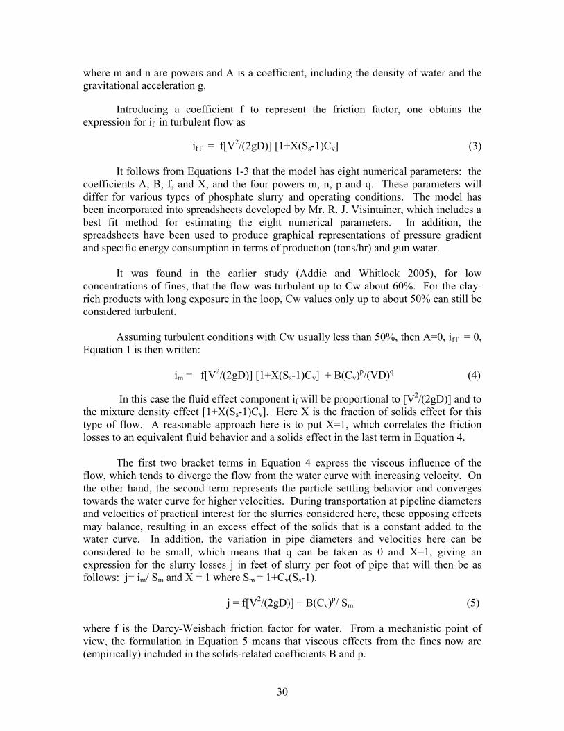
30

where m and n are powers and A is a coefficient, including the density of water and the gravitational acceleration g.

Introducing a coefficient f to represent the friction factor, one obtains the expression for if in turbulent flow as

ifT = f[V2/(2gD)] [1+X(Ss-1)Cv] (3) It follows from Equations 1-3 that the model has eight numerical parameters: the coefficients A, B, f, and X, and the four powers m, n, p and q. These parameters will differ for various types of phosphate slurry and operating conditions. The model has been incorporated into spreadsheets developed by Mr. R. J. Visintainer, which includes a best fit method for estimating the eight numerical parameters. In addition, the spreadsheets have been used to produce graphical representations of pressure gradient and specific energy consumption in terms of production (tons/hr) and gun water. It was found in the earlier study (Addie and Whitlock 2005), for low concentrations of fines, that the flow was turbulent up to Cw about 60%. For the clay-rich products with long exposure in the loop, Cw values only up to about 50% can still be considered turbulent. Assuming turbulent conditions with Cw usually less than 50%, then A=0, ifT = 0, Equation 1 is then written: im = f[V2/(2gD)] [1+X(Ss-1)Cv] + B(Cv)p/(VD)q (4)

In this case the fluid effect component if will be proportional to [V2/(2gD)] and to the mixture density effect [1+X(Ss-1)Cv]. Here X is the fraction of solids effect for this type of flow. A reasonable approach here is to put X=1, which correlates the friction losses to an equivalent fluid behavior and a solids effect in the last term in Equation 4. The first two bracket terms in Equation 4 express the viscous influence of the flow, which tends to diverge the flow from the water curve with increasing velocity. On the other hand, the second term represents the particle settling behavior and converges towards the water curve for higher velocities. During transportation at pipeline diameters and velocities of practical interest for the slurries considered here, these opposing effects may balance, resulting in an excess effect of the solids that is a constant added to the water curve. In addition, the variation in pipe diameters and velocities here can be considered to be small, which means that q can be taken as 0 and X=1, giving an expression for the slurry losses j in feet of slurry per foot of pipe that will then be as follows: j= im/ Sm and X = 1 where Sm = 1+Cv(Ss-1). j = f[V2/(2gD)] + B(Cv)p/ Sm (5) where f is the Darcy-Weisbach friction factor for water. From a mechanistic point of view, the formulation in Equation 5 means that viscous effects from the fines now are (empirically) included in the solids-related coefficients B and p.

31

Values of B and p obtained from the representation of the field and laboratory data in Figures 8-11 are summarized in Table 11. Table 11. Empirically Determined Values of B and p in Equation 5.

Matrix Type B C F Transfer B in eq.5 0.029 0.024 0.43 0.06 p in eq.5 0.28 0.28 2.6 1.2

Matrix Type D The Wingate Type D matrix, as noted earlier, is similar to Type F except that it has higher pebble and fines concentrations. A field evaluation carried out by Roy Duvall (see Appendix J) shows this to be the case. Subsequently, the slurry is to be represented by the following modelling constants: B = 0.085 p = 1.0. Tailings It is assumed that the tailings product is essentially free from fine material and that the size distribution is rather narrow, with d50 about 275 µm and maximum particle size about 500 µm. Tests conducted at GIW for various types of sand have been the background for the friction loss algorithm in the GIW Slysel software and have therefore been used here to define the parameters B and p in Equation 5. The result was: B= 0.075 p= 0.95. If there is a considerable portion of pebbles in the tails then the overall size distribution will be broader, which may compensate for a larger average particle size (i.e., the B and p values above may still simulate the losses reasonably well). This will be covered in the discussion section of this report. Clay The clay model is mainly based on GIW tests. For laminar flow, the pipe wall shear stress or the friction losses are empirically related to the scaling parameter 8V/D including a yield stress, as shown earlier in Figure 6. The pumping of clay takes place at fairly low velocities in large-diameter pipelines, which means that the scaling parameter 8V/D will normally be in the range of 10-40. In this region, the wall shear stress is not linearly related to the scaling parameter, and Equation 2 for the general model has been adapted with values of A, m, and n determined from measured data (see Figure 12).

32

Estimated yield stresses formed the background to which a criterion can be applied (Sellgren and Wilson 2007) for the transition velocity, VT (see Figure 12). From the VT point, turbulent flow is considered to (approximately) increase with velocity in parallel with the water curve. The actual spreadsheet model is provided in Appendix H.

Figure 12. Schematic Description of Clay Friction Loss Modelling. Sand-Clay The behavior of the sand-clay mixture shown in Appendix G, up to a total sand-clay mixture SG of 1.34 and a clay SG from 1.08-1.14, showed sand-clay as having a similar flow pattern to clay. However, the addition of sand increased the friction losses considerably. In order to avoid the tendency of sand particles to settle on the bottom of the pipe, a larger velocity should be used compared to clay-only pumping. More attention has therefore been paid to larger values of 8V/D for the sand-clay mix than for the clay-only modelling. The clay-only data in the sand-clay mix tests was evaluated with constants which are not linked directly to the A, m, and n used in the clay model. An empirical relationship was also established to express the effect of adding sand by using a constant multiplied by the total slurry SG minus clay SG. Due to the principal similarity with the clay-only behavior, a similar modelling technique was used for the sand-clay model.

33

Variability Coefficient The various matrices categorized and modelled here may at times and at certain locations behave differently due to varying solids size and clay content of the in-situ matrix. Therefore a matrix variability coefficient has been introduced in the spreadsheet model. The coefficient can also be used for tails, clay, and clay-mix types to adjust the resulting values for the effect based on field experience. The variability coefficient can also be used to adjust for the actual surface condition of the pipeline. EFFECTS OF SOLIDS ON HEAD AND EFFICIENCY

The energy consumption of pumping the slurry in a pipeline system also includes the total efficiency ηT of the pumps in a system. Assume that the power lost in the motor and in the transmission corresponds to an efficiency factor ηM. Then ηT can be related to the pump efficiency,η, in the following way: η⋅η=η MT (6)

The pump head and efficiency when pumping water are generally lowered by the presence of solids. When pumping slurries, the relative reduction of the clear water head and efficiency for a constant flow rate and rotary speed may be defined by the ratios and factors shown in Figure 13.

Head ratio: HR = H/H0 Efficiency ratio: ER = η/η0 Head reduction factor: RH = 1 – HR Efficiency reduction factor: Rη = 1 – ER Figure 13. Sketch Defining the Reduction in Head and Efficiency of a Pump. In Figure 13, H and H0 are head in feet of slurry and water, respectively. Efficiencies in slurry and water service are denoted η and η0 respectively. With the definition of Rη it follows that:

34

)R1(??? ?0MT −⋅= (7) The earlier lab study (Publication No. 04-069-215) was comprised of full-size pumps and pipelines. The pump solids effect on head was negligible even for the highest concentration investigated for the clay-rich matrix which had friction loss gradients over 0.1. The pump solids effect on efficiency for these slurries at 60w% was up to R?, about 13%. The data collected during the field evaluations reported here at high concentrations resulted in low gradients (Figure 9). R? was about 10%, which included the effect of operating with worn pump parts. R? can be related approximately linearly to the solids concentration by weight. The reduction in efficiency is then expressed in the following way with Cw in percent. R? = 10(Cw/60) (8) For example, R? = 7.5% for Cw= 45% gives a multiplication factor of 0.925 to be applied against the pump’s water efficiency.

35

USE OF THE EXCEL SPREADSHEET To begin using the spreadsheet, go to the worksheet titled “Input.” The spreadsheet should open to this location. First, choose the model you will be using from the green highlighted drop-down box. Nine models are available (Type B, Type C, Type D and Type F Matrix, Transfer Matrix, Phosphate Tailings, Phosphate Clay and Clay-Sand Mix). The Matrix models are selectable by mine name and the type letters can be correlated against a Feed-Pebble-Fines chart seen on the right-hand side of this worksheet. All cells highlighted in yellow are input cells. All other cells are fixed or calculated; they are protected and cannot be altered. Most inputs have an allowable range. If this range is exceeded, red highlighted text will appear to point out the over-range values. Over-range values will not be plotted in the output. (Limits have been selected according to the available data and other theoretical considerations. For more detail, consult the project reports.) Inputs Include: Titling. This is for information only and appears on all of the plots. Fluid SG. Currently limited to 1.0 (water) for all models except Sand-Clay. Pipe diameter. Limits for each model are given above the entry box. Pipe length. Used to calculate total Pipeline Head. Variability Coefficient. This is a user defined coefficient that allows the results of the spreadsheet to be adjusted to match local experience and variability in the composition of the solids. It is valid for all models and is multiplied directly into the calculated friction loss value (j and iM). The default value of 1.0 should be used if there is no better information available. If a value other than 1.0 is selected, it will be displayed on the output sheets. Lines of constant CW. These will be plotted on all of the output plots. Lines of constant mixture velocity V. These will be plotted on the Velocity version of the Specific Energy plot. Lines of constant gun water. These apply to the matrix models only and will be plotted on the Gun Water version of the Specific Energy plot.

36

Matrix moisture. This applies to the matrix models only and is needed to complete the gun water calculations. Output Plots Include: iM plot. Friction Loss iM (ft water/ft) against Mixture Velocity V (ft/sec) at various CW (%). J plot. Friction Loss J (ft slurry/ft) against Mixture Velocity V (ft/sec) at various CW (%). GPM plot. Pipeline Head (ft slurry) against Flowrate (gpm) at various CW (%). V plot. Specific Energy Consumption (hp-hr/ton-mile) against Production (tons/hr) with lines of constant CW (%) and V (ft/sec). Gun Water plot. Specific Energy Consumption (hp-hr/ton-mile) against Production (tons/hr) with lines of constant CW (%) and Gun Water (gpm). GENERAL NOTES FOR USING THE EXCEL SPREADSHEET Microsoft Excel is required. The spreadsheet contains macros, and macros must be enabled for it to work properly.

Some functionality may be lost if older versions of Excel are used. If problems occur, try installing system updates or updating to a later version. SPREADSHEET PROTECTION The spreadsheet is protected to prevent accidental alteration of fixed text and calculations. It is highly recommended that the spreadsheet be left in this state during normal use to prevent corruption of the calculations or text. Protection can, however, be disabled (worksheet by worksheet) by going to the “Tools” menu, selecting “Protection,” and then “Unprotect Sheet.” There is no password. There are also several hidden worksheets where the individual models are calculated. These can be unhidden by going to the “Format” menu, selecting “Sheet,” then “Unhide.” There are also several hidden lines on the “Input” worksheet. These can be un-hidden by highlighting all of the rows on this sheet, going to the “Format” menu, selecting “Row,” then “Unhide.”

37

There are two macros included with this spreadsheet for instantly unprotecting and unhiding all worksheets: CTRL "u" unprotects and unhides all sheets and hidden rows so the spreadsheet can be altered. CTRL "p" protects all sheets, hides the calculation sheets and hides some special rows on the INPUT sheet to prepare the spreadsheet for normal use. Programmer’s Note: If rows are added or subtracted from the INPUT sheet, it may be necessary to adjust the VB code for these macros accordingly so that the correct rows are hidden.

39

EXCEL SPREADSHEET RESULTS AND GRAPHICAL OUTPUT The results of all the different tests are provided in the form of the Excel spreadsheet and plots. These are printed out in full in Appendix H. A CD of the spreadsheet is attached. The spreadsheets are set up so that values such as Solids SG, Fluid SG, Pipeline Diameter, Solids Concentration, etc., are in yellow and may be varied as necessary. The spreadsheet has an input tab which directs the user to the appropriate matrix type based on the mine location for Types B, C, and F. The input tab also enables the user to select from transfer type matrix, sand-clay mix, clay only, and tails slurries. Model constants for the input sheet are set as outlined in the Hydraulic Analysis and Modelling Section of this report. The required high pressure water (gun water) used to break down the matrix in the pit is also determined and related to the pumped solids content based on an assumed water content in the matrix. Resulting water contents from F and B samples were about 15 and 20%, respectively (Zaman 2005). Graphical output is provided for each of the different noted types. For example, a plot for the hydraulic gradient j in feet of mixture per foot of pipe for the Type F matrix as shown in Figure 14 (below) is provided. The Excel model also provides a separate sheet with output in terms of im, in feet of water per foot of pipe.

Figure 14. Head Loss Versus Velocity Plot.

40

The specific energy consumption versus tons per hour of dry solids transported is also shown with different constant concentrations and mean mixture velocities or with constant gun water.

Figure 15. Energy Versus Production Plot with Cw and Velocity.

Figure 16. Energy Versus Production with Cw and Gun Water.

41

Here it should be noted that in the case of transfer, tails, sand-clay mix, and clay-only matrix types that the gun water plots have been deleted. Below are some clay and clay-mix results for comparison with modelled values. Note: the limitations of operating conditions are given as comments on the attached Excel model spreadsheets. Clay model results have been used here to compare two systems with the same capacity in dry solids: one with 4w% in a 19” pipeline at 3 fps and the other for 15w% at 9.2 fps in an 8” pipeline. The gradient in feet of slurry for the large diameter system was 1.1 feet per 1,000 foot horizontal pipeline while the corresponding value in the 8” system was 53 feet. The amount of water transported in the high concentration system is less than 25% of the water in the large system. In the case of the sand-clay mixture, it should be noted that while the tests were carried out in a 3” pipe with different sand contents against a 1.08-1.14 SG clay carrier, the test results have been used to directly model the flow in a large-scale application with a velocity of 6 fps in a 19” pipeline in the example below. Clay Clay + Sand Slurry S.G. 1.08 1.28 Friction loss gradient, j: 0.01 0.019 Slurry S.G. 1.14 1.34 Friction loss gradient, j: 0.035 0.046 It follows that the head requirement (i.e., j), is nearly doubled when adding sand up to an S.G. of 1.28 in a clay slurry with an S.G. of 1.08. With a slightly larger SG of 1.34, the head requirement is about 2.5 times larger when the clay SG is 1.14. The increase is mainly related to the comparatively large increase in the resistance to flow from the larger clay portion. In the sand-clay example, the flows tended to be laminar, which means that larger sand particles may deposit on the bottom of the pipe.

43

DISCUSSION PIPELINE PUMPING The field results for Types B and C indicated that the pumping head requirement (i.e., the gradient j), could be considered to be constant up to very high solids concentrations. The favorable outcome of this is expressed in Table 12 for a Type C matrix being transported in a 21” diameter pipeline when considering operation at higher concentrations for 16 fps. Table 12. Evaluation of Increased Capacity Effects on Water and Energy Savings.

Solids Cw% 30 45 60 Water req. gal/ton 1485 777 467 Capacity, tons/hr 1595 2702 4140 Energy requirement (Hp-hr/ton-mile) 0.62 0.42 0.31

It follows from Table 12 that an increase in Cw from 30 to 60% reduces the energy consumption required to overcome pipeline friction by half and reduces the water requirement by more than two-thirds. In addition, the capacity in dry tons increases 2.6 times with the higher concentration. The favorable pumping conditions for the Type C matrix in Table 12 may be related to a seemingly well-balanced particle size distribution within the pipeline with pebbles and fines content of about 25% and 15%, respectively. Similar distributions are expected for Type B. PIT OPERATION Operation at higher concentrations means that limitations imposed by the pit must be considered. Here the solids must be slurried and enter the first pit pump suction. The drag line usually dumps semi-dry solids on the side of the pit where water jets are used to drift it through a 6” spaced grizzly into the pit. The slurry then gravitates to the suction pipe end located near the bottom of the pit and the suction vacuum at its entrance draws the slurry into the suction pipe and pump. In the past, the slurry pumps used at the pit cavitated at about 35% Cw, limiting the solids concentrations at which they could be consistently and reliably operated. The new generation of slow-running, improved suction LSA 62” pumps have eliminated (for the most part) this limitation, allowing cavitation-free operation up to around 60w%. This is seen in the evaluation test data.

44

The drifting of the slurry through the grizzly into the pit currently utilizes large quantities of high-pressure water. If energy savings are to be achieved, this water consumption must be reduced and controlled. It has been shown that at times gun water can be reduced. Unfortunately there is limited or no control here and a methodology does not exist to reduce gun water on a consistent basis. Work is currently being done on this at PCS Phosphate North Carolina by Hagler Systems of North Augusta, SC. A presentation on the status of this work is included as Appendix I. FLOW MECHANISMS The favorable operating conditions shown in Table 12 (above) are typical for broad particle grading and do not necessarily rely on a content of very fine particles (see Figure 17).

Figure 17. Friction Losses for Cw from 40 to 64% (Sand 3). It follows from Figure 17 that the friction loss remained approximately constant in feet of slurry per foot of pipe when the solids concentration was increased from 40 to

45

64w%. The average particle size was about 600 micron, with a negligible amount smaller than 40 micron. The important role of particles with sizes 0.1 to 0.5 in diminishing friction was pointed out by Sundqvist and others (1999). With the narrower sands in Figure 17, there was an increase in the friction loss gradient, j, with increased concentrations. Sometimes “mud (clay) balls” of substantial diameter are formed during the matrix pipeline pumping. The estimated variations in particle size distributions for pumped matrices are schematically summarized in Figure 18.

Figure 18. Estimated Span of Particle Size Distributions for Pumped Matrix Ore. Clay balls can be formed when clay rich matrix enters the pit pump. There are no indications in the literature of increased friction related to clay balls. It has been discussed earlier how settling and non-settling friction loss mechanisms seem to balance when pumping matrices. This balance of the partly opposing settling and non-settling effects formed the overall background for the simplified modelling approach adopted here, as discussed in connection with equation 5 and shown schematically in Figure 19.

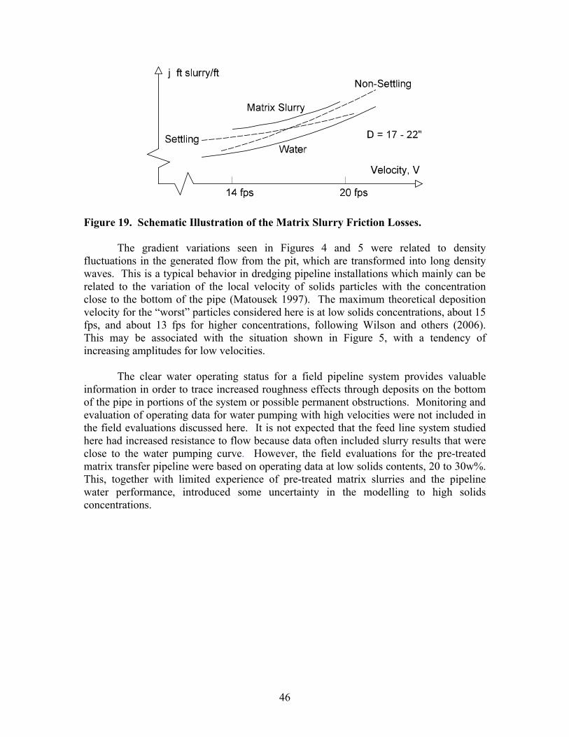
46

Figure 19. Schematic Illustration of the Matrix Slurry Friction Losses. The gradient variations seen in Figures 4 and 5 were related to density fluctuations in the generated flow from the pit, which are transformed into long density waves. This is a typical behavior in dredging pipeline installations which mainly can be related to the variation of the local velocity of solids particles with the concentration close to the bottom of the pipe (Matousek 1997). The maximum theoretical deposition velocity for the “worst” particles considered here is at low solids concentrations, about 15 fps, and about 13 fps for higher concentrations, following Wilson and others (2006). This may be associated with the situation shown in Figure 5, with a tendency of increasing amplitudes for low velocities. The clear water operating status for a field pipeline system provides valuable information in order to trace increased roughness effects through deposits on the bottom of the pipe in portions of the system or possible permanent obstructions. Monitoring and evaluation of operating data for water pumping with high velocities were not included in the field evaluations discussed here. It is not expected that the feed line system studied here had increased resistance to flow because data often included slurry results that were close to the water pumping curve. However, the field evaluations for the pre-treated matrix transfer pipeline were based on operating data at low solids contents, 20 to 30w%. This, together with limited experience of pre-treated matrix slurries and the pipeline water performance, introduced some uncertainty in the modelling to high solids concentrations.

47

SUMMARY OBSERVATIONS

The specific energy consumption to overcome pipeline friction losses for Type B and C at 60w% was about 0.34 and 0.31 hp-hr/ton-mile, respectively, when pumped at 16 fps in a 21” pipeline. The corresponding value for Type F was 0.38. Slurry data collected on two different occasions at the Lonesome Train 18 pipeline are modelled here as Type C matrix. The data indicates operating at higher concentration (about 60w%) would result in a more efficient operation. An increase from 30 to 60w% reduces the energy consumption required to overcome pipeline friction by half and reduces the water requirement by more than two-thirds. In addition, the capacity in dry tons increases 2.6 times with the higher concentration. The favorable pumping conditions may be related to a seemingly well-balanced particle size distribution during the pumping. A similar behavior was observed during field tests conducted at South Ft. Meade (Type B matrix). Field and large-scale loop test results for Type F matrix slurries with a fines content well below 15% and negligible pebble content showed that F matrix slurries also can be pumped effectively at 60w%. The field evaluations of the pump performance in matrix slurry pumping indicated, together with earlier full-scale laboratory results, that the reduction in efficiency, including the influence of successive wear, increases in proportion to the solids concentration to be about 10% at 60w%. For example, with Cw= 45% the water efficiency of the pump is reduced through multiplication with a factor of 0.925. The reduction in head can be considered to be negligible. The composition of the ore that reaches the pumping pit depends on both the local geological background and the handling up to the pit. A clay-rich matrix (Type B or C) that breaks up easily and liberates the fines quickly during pumping may have losses similar to a matrix with a long exposure time in the closed loop lab tests. Under such conditions, pumping concentrations should preferably be less than 50w% maximum based on the capabilities of typical pumping installations. The average fines content published in the geological surveys at the various listed mining locations seem in practice to correspond to average maximum values of about 25% when pumped. The result indicates that the screening that takes place in the mining and handling up to the pit is a leading factor for effective pumping, provided that the pit operation does not impose restrictions. When operating at higher concentrations, limitations imposed by the pit must be considered. The handling in the pit and the use of gun water shall be seen from the perspective of the new generation of slow-running pumps allowing cavitation-free operation up to around 60% by weight.

48

The gun water flow rate is calculated for the matrix flow modelling. The corresponding energy consumption depends on the pressure requirement and the transportation to the pit. With free surface gravity flow, a considerable amount of water is lost through evaporation. The results for clay-only and sand-clay mixtures demonstrated the strong effect of the clay content on the friction losses for clay concentrations over a few percent.

49

CONCLUSIONS

Tests, analysis, and spreadsheet development have been carried out for different types of matrix (transfer matrix, tails, sand-clay mix, and a clay-only type of phosphate slurry). Excel spreadsheets and models with graphical output have been developed for all of these and are made available in this report. A way of selecting the different matrix models and other types of slurries is provided such that a mine planner can use them for a variety of different pipeline diameters, concentrations, and other cases. As laid out, it is hoped the spreadsheet will cover all the phosphate mine planners’ pumping pipeline friction needs. All of the model plots provide the ability to evaluate energy consumption for different scenarios. The matrix models include special plots that show how gun water needs to be controlled to reduce pumping costs. The models, and in particular the plots, indicate that significant savings are possible by tailoring the operation to the specific matrix type. The test data collected verifies this is possible from a pumping point of view.

51

REFERENCES

Addie GR. 1989. Phosphate matrix pipeline design data and tools for efficiency improvement. Bartow (FL): Florida Institute of Phosphate Research. Publication nr 04-037-078. Addie GR, Hagler TW. 1989. Potential operating cost improvements in Florida matrix transportation. Paper presented at: Environmental Education from the Ground Up: an AIME/AIChE/AIPG/FIPR regional phosphate conference; 1989 Oct 27-28; Lakeland, FL. Addie GR, Whitlock L. 2001. Matrix pump performance evaluation while cavitating. Bartow (FL): Florida Institute of Phosphate Research. Publication nr 04-069-215. Addie GR, Whitlock L. 2005. Centrifugal slurry pump concentration limit testing and evaluation: Phase I. Bartow (FL): Florida Institute of Phosphate Research. Publication nr 04-069-215. Matoušek V. 1997. Flow mechanism of sand-water mixtures in pipelines [DPhil dissertation]. Netherlands: Delft University. 258 p.

Scott T, Courtney J. 2006. The southern extension of the Central Florida phosphate district - a stratigraphic discussion and future mining plans. Unpublished paper presented at the 21st Annual Regional Phosphate Conference; 2006 Oct 11-12; Lakeland, FL.

Sellgren A, Wilson KC. 2007. Validation of a four-component pipeline friction loss model. In: Proceedings, 17th International Conference on Hydrotransport; 2007 May 7-10; Capetown, South Africa. Sundqvist A, Sellgren A, Addie GR. 1999. Pipeline friction losses of coarse sand slurries. Powder Technology 89: 8-9. Wilson KC, Addie GR, Sellgren A, Clift R. 2006. Slurry transport using centrifugal pumps. New York: Springer. Wilson KC, Visintainer RJ. 2006. Modelling pipeline flow of non-Newtonian slurries with settling particles. In: Proceedings, 13th International Conference on Transport and Sedimentation of Solid Particles; 2006 Sep 18-20; Tbilisi, Republic of Georgia. Zaman A. 2005. Characterization of phosphate slurries for pump effects and pipe effects. Bartow (FL): Florida Institute of Phosphate Research. Publication nr 04-04-070.