CENTRIFUGAL COMPRESSOR DIFFUSER ROTATING STALL: … · Centrifugal compressor diffusers rotating...
12
Paper ID: ETC2017-157 Proceedings of 12th European Conference on Turbomachinery Fluid dynamics & Thermodynamics ETC12, April 3-7, 2017; Stockholm, Sweden OPEN ACCESS Downloaded from www.euroturbo.eu 1 Copyright © by the Authors CENTRIFUGAL COMPRESSOR DIFFUSER ROTATING STALL: VANELESS VS. VANED M. Giachi a * - E. Belardini a - G. Lombardi b - A. Berti b - M. Maganzi c a GE Oil&Gas, Florence, Italy b University of Pisa - Dept. of Civil and Industrial Engineering - Aerospace Section, Pisa, Italy c CUBIT s.c.a.r, Pisa, Italy * Corresponding author, email: [email protected] ABSTRACT Diffuser rotating stall (in both cases of a vaneless or a vaned configuration) is still one of the open questions which has never been fully understood because of the complexity of the phenomenon and the experimental difficulties to get reliable measurements in such a complex environment. Under this perspective, Computational Fluid Dynamics (CFD) is an interesting tool to "see" the flow and to provide a basic understanding of the associated physics. Several published work have shown that a simplified model of the diffuser without the upstream impeller and the downstream return channel, with some realistic boundary conditions entering the diffuser, can provide a qualitative analysis of the stall onset. Thanks to the simplified model it has been possible to change progressively the boundary conditions in such a way that the continuous reduction of flow in time, as it is the experimental procedure, has been fully simulated. Vaneless and vaned options have been compared. Nomenclature AR diffuser aspect ratio (AR=b 4 /R 2 ) b diffuser width (mm) Cp pressure coefficient Cp (R) =(p (R) -p 2 )/P 2 -p 2 ) f frequency (1/sec) f r reduced frequency f/1xREV p static pressure (Pa) P total pressure (Pa) R radius (mm) Re Reynolds number Re=V 2 ·b 4 · ~·0.00295·15.8/0.0000175=1.9·10 5 U impeller peripheral speed (m/sec) V absolute gas velocity (m/sec) Greek letters flow angle from tangential (°degs) loss coefficient R) P 2 -P (R) )/(P 2 -p 2 ) vorticity (1/sec) Subscripts CFD from CFD results r radial t tangential m mean VL vaneless case VD vaned case 2 impeller outlet 4 diffuser outlet
Transcript of CENTRIFUGAL COMPRESSOR DIFFUSER ROTATING STALL: … · Centrifugal compressor diffusers rotating...

Paper ID: ETC2017-157 Proceedings of 12th European Conference on Turbomachinery Fluid dynamics & Thermodynamics ETC12, April 3-7, 2017; Stockholm, Sweden
OPEN ACCESS Downloaded from www.euroturbo.eu
1 Copyright © by the Authors
CENTRIFUGAL COMPRESSOR DIFFUSER ROTATING STALL:
VANELESS VS. VANED
M. Giachia* - E. Belardini
a - G. Lombardi
b - A. Berti
b - M. Maganzi
c
aGE Oil&Gas, Florence, Italy
bUniversity of Pisa - Dept. of Civil and Industrial Engineering - Aerospace Section, Pisa, Italy
cCUBIT s.c.a.r, Pisa, Italy
*Corresponding author, email: [email protected]
ABSTRACT
Diffuser rotating stall (in both cases of a vaneless or a vaned configuration) is still one of the
open questions which has never been fully understood because of the complexity of the
phenomenon and the experimental difficulties to get reliable measurements in such a complex
environment. Under this perspective, Computational Fluid Dynamics (CFD) is an interesting
tool to "see" the flow and to provide a basic understanding of the associated physics. Several
published work have shown that a simplified model of the diffuser without the upstream
impeller and the downstream return channel, with some realistic boundary conditions entering
the diffuser, can provide a qualitative analysis of the stall onset. Thanks to the simplified model
it has been possible to change progressively the boundary conditions in such a way that the
continuous reduction of flow in time, as it is the experimental procedure, has been fully
simulated. Vaneless and vaned options have been compared.
Nomenclature
AR diffuser aspect ratio (AR=b4/R2)
b diffuser width (mm)
Cp pressure coefficient Cp(R)=(p(R)-p2)/P2-p2)
f frequency (1/sec)
fr
reduced frequency f/1xREV
p static pressure (Pa)
P total pressure (Pa)
R radius (mm)
Re Reynolds number Re=V2 ·b4·~·0.00295·15.8/0.0000175=1.9·105
U impeller peripheral speed (m/sec)
V absolute gas velocity
(m/sec)
Greek letters
flow angle from tangential (°degs)
loss coefficient R)P2-P(R))/(P2-p2)
vorticity (1/sec)
Subscripts
CFD from CFD results
r radial
t tangential
m mean
VL vaneless case
VD vaned case
2 impeller outlet
4 diffuser outlet
2
INTRODUCTION
Centrifugal compressor diffusers rotating stall is still an open question in the radial machine community
and in the most of the cases the know-how is limited to the critical angle at which a rotating
phenomenon occurs. There are examples of some analytical approach to the problem of diffuser
stability done in the past as the one by Jansen (1964). However, they have never arrived at a practical
application and, typically, the problem has been investigated experimentally always with large
difficulties even considering the most advanced experimental techniques as described in Camatti et al.
(1997), Ferrara et al. (2004), Gau et al. (2007) and Bianchini et al. (2014), Bianchini et al. (2015),
Dazin et al. (2015). It is a matter of fact, that the “historical” definition by Kinoshita & Senoo (1985) of
the critical flow angle has still a fundamental role in the industrial environment, as discussed by Fulton
& Blair (1995) and the theory is left to manuals and textbooks as the one by Japikse (1996). Vaned
diffuser rotating stall has been also studied by Benichou et al. (2016), Dodds et al.(2015), Ješe et
al.(2015). Having said that, CFD appears to be an intersting tool to understand something more about
the physics of diffuser rotating stall and to produce useful information about viscous losses and flow
separation which can be used to develop again some analytical model with new inputs from numerical
analysis. CFD is not an easy task because one needs to solve heavy, time-dependent, three-dimensional
Navier Stokes equations but nowadays it can be done both running the entire stage as done by
Marconcini et al. (2016) and Pavesi et al. (2011) or running a simplified model of the diffuser alone as
done by Ljevar et al. (2006), Ljevar (2007). The simulations with the simplified model have been
performed in a 2D environment assuming that in case of wide diffuser the wall boundary layers play a
minor role and a core instabiltiy occurs which can be studied in the framework of a simplified 2D
assumption. Boundary conditions are kept fixed at a given flow angle and several runs are performed at
different flow angles to identify the critical value of flow angle at which some rotating cells develop. In
the present work a simplified model approach has been applied but the model is a full three-
dimensional model of the diffuser and the downstream 180° degs U-bend. The velocity profiles coming
from the usptream impeller, which is not included in the model, have been applied at the inlet of the
computational domain and, thanks to the (relatively) simplicity of this approach, the boundary
conditions have been changed in time to simulate the experimental procedure where the throttling valve
is progressively closed to reduce continuously the flow angle from design point to stall onset as already
described in Giachi et al. (2016). The major advantage of this approach is the possibility of following
continuously the stall onset and the rotating cells development. This is even more important in case of
vaned diffuser where the wakes of the vanes are expected to play an important role. The rotating stall
mechanism is even less understood in case of vaned diffuser which are relatively easy to design in order
to get good performance but with a significant operating range reduction as shown in Camatti et al.
(1995). In this paper, the flow behavior and performance of a vaned diffuser are also described.
GEOMETRY
The numerical domain is shown in Fig.1 from the exit of the impeller to the end of the 180°degs U-
bend. The diffuser aspect ratio AR=0.015 classifies the current diffuser as a "thin" diffuser where, in
principle, the hub and shroud boundary layers are expected to play a role in the stability of the flow.
The vane is obtained from a traditional NACA airfoil without any special study or treatment and the
incidence has been preliminarly adjusted to have a smooth flow with no separation close to design
point.
Numerical model
The analysis has been done using a commercial software based on Reynolds Averaged Navier-Stokes
model run in an incompressible and unsteady mode (URANS). The grids for the vaneless case and the
vaned one contain 35 and 51 millions of trimmed cells respectively with 11 prismatic layers with a
stretching factor of 1.1 for a resulting total thickness of 1.3 mm at both walls, hub and shroud.
3
Figure 1: Main dimensions of the diffuser channel and blade profile
The turbulence model is a standard realizable k- with a two-layer all y+ model having assumed an
intensity i=1% and a viscosity ratio of 10. The time step is 0.0002 sec. which corresponds to a
frequency of 5 kHz i.e. three times the passing frequency of the blades having assumed that the blade
passing frequency is the highest frequency of interest.
Before running the final cases some preliminary tests were done to get confidence with such a new
simulation in a simplified 2D case. The main conclusion, shown in Fig.2, is that below a certain critical
angle a rotating phenomenon always occurs even (and this was the most surprising to us) even in a 2D
case without any kind of boundary layers at the walls and with an uniform inlet flow without any jet-
wake flow distortion.
Figure 2: Preliminar runs to check the effect of the numerical discretization on the presence of
rotating instability
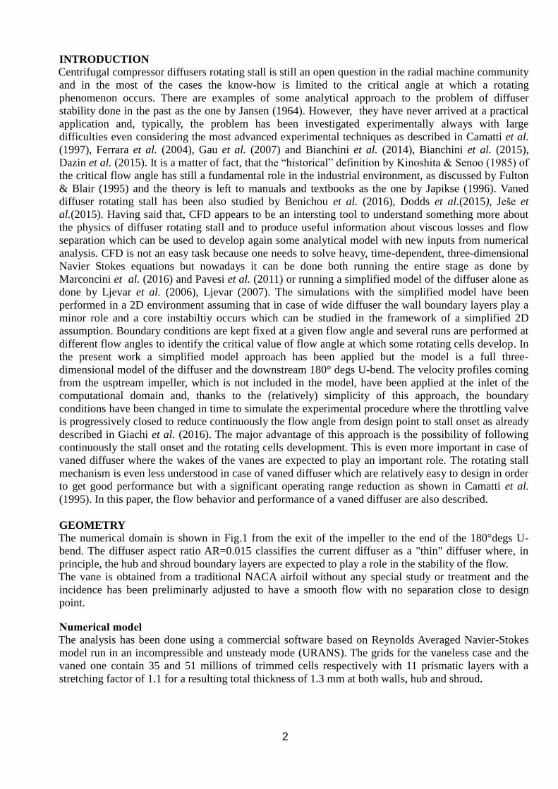
The grid sensitivity has been repeated for the 3D case running a 250 millions node fine grid and a
coarse grid, as shown in Fig.3, as well as a turbulence model sensitivity check (realizable k- and k-
SST). In both cases no significant effects have been found .
Figure 3: Grid sensitivity on 3D case (top): fine (left), coarse (right) as used for this work. The
purpose of the figure is to show the grid. The details of the pinch region are not relevant.

4
Boundary conditions
The boundary conditions have been assigned in terms of the inlet velocity profiles at section 2 and
the outlet mean value of the static pressure at the outlet of the computational domain.
The inlet velocity profiles have been derived from a preliminary steady calculation on the whole stage
(impeller, diffuser and return channel) as shown in Fig.4. They represent a typical profile where the
flow coming from the impeller is visible as well as the flow from hub and shroud cavities and the
blockage due to the hub/shroud wall thickness.
A certain amount of blockage at the exit of the impeller has been taken into account assuming no radial
velocity and a tangential velocity equal to the impeller rotational speed (U2=76.8 m/sec) in 24 sectors
approximately 2 degrees each. In Fig.5 an overall view of the velocity distribution is given as it appears
from an external point of view where the blockage corresponds to a 13% reduction of the exit area of
the impeller. The whole set of boundary conditions is rotating at the peripheral speed of the impeller
which corresponds to a 1xREV frequency f1xREV=62.5 Hz and a disturbance passing frequency of 1.5
kHz. The simulation covers 15 seconds in time in which the radial component of the absolute velocity
entering the diffuser is continuously reduced and the tangential component is increased in order to
replicate the testing procedure where, in fact, the throttling valve is progressively closed from the
design flow down to the minimum sustainable flow immediately before surge as shown in Fig.6. The
duration of the test is much longer (10 min approximately) than the numerical simulation (15.6
seconds), but it has been assumed a quasi-steady conditions where the speed of the closure of the valve
is not relevant. This assumptions is supported by the fact that there are several orders of magnitude
between the velocity of a rotating stall (between 0.16-0.32 seconds for one revolution) and the velocity
of the valve closure (0.2° degs/sec) which means that the flow angle changes of approximately 0.03°
degs only in one revolution.
The gas is nitrogen at a diffuser inlet conditions of 14 bar and 25 °C. The Reynolds number in such
conditions referred to diffuser width and diffuser inlet absolute velocity is 1.9·105
Figure 4: Velocity profiles (typical) from the impeller as computed by CFD (top) and simplified
applied boundary conditions: radial velocity (bottom left) and tangential velocity (bottom
right). Dark regions indicate the flow coming from the impeller
5
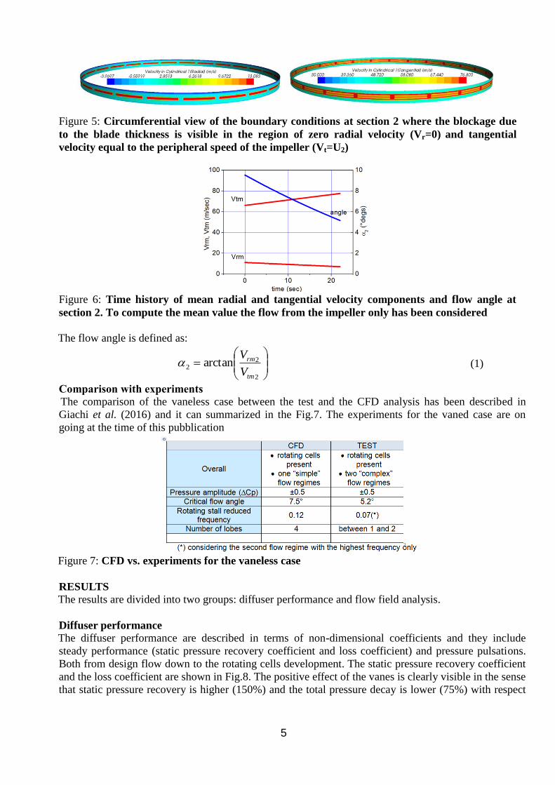
Figure 5: Circumferential view of the boundary conditions at section 2 where the blockage due
to the blade thickness is visible in the region of zero radial velocity (Vr=0) and tangential
velocity equal to the peripheral speed of the impeller (Vt=U2)
Figure 6: Time history of mean radial and tangential velocity components and flow angle at
section 2. To compute the mean value the flow from the impeller only has been considered
The flow angle is defined as:
2
22 arctan
tm
rm
V
V (1)
Comparison with experiments
The comparison of the vaneless case between the test and the CFD analysis has been described in
Giachi et al. (2016) and it can summarized in the Fig.7. The experiments for the vaned case are on
going at the time of this pubblication
Figure 7: CFD vs. experiments for the vaneless case
RESULTS
The results are divided into two groups: diffuser performance and flow field analysis.
Diffuser performance
The diffuser performance are described in terms of non-dimensional coefficients and they include
steady performance (static pressure recovery coefficient and loss coefficient) and pressure pulsations.
Both from design flow down to the rotating cells development. The static pressure recovery coefficient
and the loss coefficient are shown in Fig.8. The positive effect of the vanes is clearly visible in the sense
that static pressure recovery is higher (150%) and the total pressure decay is lower (75%) with respect

6
to the vaneless configuration. This gives an overall increase in the efficiency of the stage. It is
remarkable the fact that the static pressure increase is higher than the total pressure decay reduction.
This is due to the fact that the flow angle in the diffuser is changed, thanks to the effect of the vanes,
and the pressure recovery increases according to the effect of the flow angle 4 according to where, for
CFD expression, all quantities are mass averaged values:
CFDCFD
CFDCFDCFD
pstPtot
pstpstCp
22
24
(2a)
CFD
CFD
CFDTheoryD
A
ACp
2
44
221
sin
sin1 (2b)
CFDCFD
CFDCFDCFD
pstPtot
PtotPtot
22
42
(2c)
Figure 8: Diffuser performance in terms of non-dimensional quantities, static pressure recovery
coefficient (left) and loss coefficient (right)
The simple model given in (2b), shown in Fig.8, confirms that the main effect of the vanes is to
change the flow angle in the diffuser and it can be well captured by a simple 1D-model. On the other
hand, stall behavior is impossible to predict by means of such a simple model and experiments are
still needed. In order to detect the stall limit the pressure pulsations in the diffuser at a radius R=220
mm have been monitored during the simulation having introduced in the model a virtual probe
(shown in Fig.1) as it is done in the test and the signal has been processed applying Wavelet theory.
Both the signals and the spectra analysis are shown in Fig.9. Rotating stall occurs at low flow angle
hence in the figures the “normal” operating condition are on the right of the plot.
In case of the vaneless diffuser the pulsations show a frequency of 30 Hz and a stall onset at
crVL=7.5 °degs with a regular increase of the pulsations amplitude. The vaned configuration is not so
simple. There are at least two different regions and the critical flow angle is higher at crVD=8.3 °degs. The two regions show a clear evolution from a low frequency phenomenon at 5 Hz (7.3°
degs<VD<8.3° degs) to a more complex situation (6.2° degs<VD<6.9° degs). In between (6.9°
degs<VD<7.3° degs) a transitional region where the frequency increases. The two different regimes
correspond to a first blade wakes instability without the presence of real well-defined stall cells and a
final state with three evident rotating cells.
7
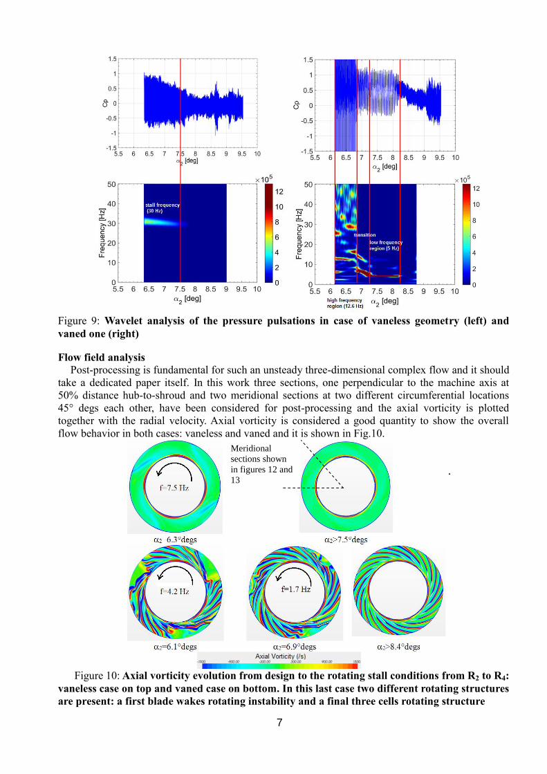
Figure 9: Wavelet analysis of the pressure pulsations in case of vaneless geometry (left) and
vaned one (right)
Flow field analysis
Post-processing is fundamental for such an unsteady three-dimensional complex flow and it should
take a dedicated paper itself. In this work three sections, one perpendicular to the machine axis at
50% distance hub-to-shroud and two meridional sections at two different circumferential locations
45° degs each other, have been considered for post-processing and the axial vorticity is plotted
together with the radial velocity. Axial vorticity is considered a good quantity to show the overall
flow behavior in both cases: vaneless and vaned and it is shown in Fig.10.
Figure 10: Axial vorticity evolution from design to the rotating stall conditions from R2 to R4:
vaneless case on top and vaned case on bottom. In this last case two different rotating structures
are present: a first blade wakes rotating instability and a final three cells rotating structure
Meridional
sections shown
in figures 12 and
13
8
In Fig.10 the smooth behavior of the vaneless case is clearly visible on bottom and one can see the
evolution from a potential (zero vorticity) flow in regular conditions (2>crVL=7.5°degs) to the
occurrence of rotating instability. There are four lobes rotating at a frequency of fVL=30/4=7.5 Hz
which, in terms of reduced frequency, corresponds to frVL=0.12. In case of the vaned geometry the
scenario is more difficult even because the location of the virtual probe is sensitive to the wakes of
the vanes. However three different flow regimes are evident as already mentioned. The wakes of the
blades become unstable and the instability start to rotate at 8.4 °degs then a transition regime and the
final stable flow fields with three rotating cells.
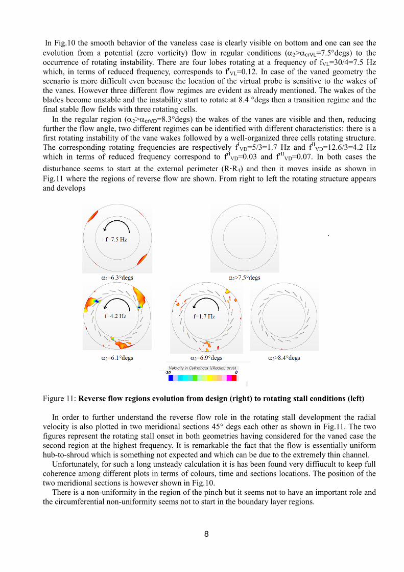
In the regular region (2>crVD=8.3°degs) the wakes of the vanes are visible and then, reducing
further the flow angle, two different regimes can be identified with different characteristics: there is a
first rotating instability of the vane wakes followed by a well-organized three cells rotating structure.
The corresponding rotating frequencies are respectively fIVD=5/3=1.7 Hz and f
IIVD=12.6/3=4.2 Hz
which in terms of reduced frequency correspond to frI
VD=0.03 and frII
VD=0.07. In both cases the
disturbance seems to start at the external perimeter (R˜R4) and then it moves inside as shown in
Fig.11 where the regions of reverse flow are shown. From right to left the rotating structure appears
and develops
Figure 11: Reverse flow regions evolution from design (right) to rotating stall conditions (left)
In order to further understand the reverse flow role in the rotating stall development the radial
velocity is also plotted in two meridional sections 45° degs each other as shown in Fig.11. The two
figures represent the rotating stall onset in both geometries having considered for the vaned case the
second region at the highest frequency. It is remarkable the fact that the flow is essentially uniform
hub-to-shroud which is something not expected and which can be due to the extremely thin channel.
Unfortunately, for such a long unsteady calculation it is has been found very diffiucult to keep full
coherence among different plots in terms of colours, time and sections locations. The position of the
two meridional sections is however shown in Fig.10.
There is a non-uniformity in the region of the pinch but it seems not to have an important role and
the circumferential non-uniformity seems not to start in the boundary layer regions.

9
Figure 12: Radial velocity for vaneless geometry (top) and vaned one (bottom)
The flow uniformity in hub-to-shroud direction is further investigated in Fig.13 where the axial
vorticity is shown again but with a different scale and in different sections. The data are availble for
the vaneless case only. In the figure a certain degree of boundary layer instability is visible but at a
very low flow angle and it seems that it is not responsible of rotating stall occurrence.
Figure 13: Axial vorticity for vaneless geometry: detailed view of the diffuser channel
The region of the pinch for the vaneless case is shown in details in Fig.14 where a reverse flow
bubble is visible. This separation bubble is a consequence of the sudden jet expansion in the non-
symmetrical volume of the pinch but it has a very minor impact on the overall flow field.
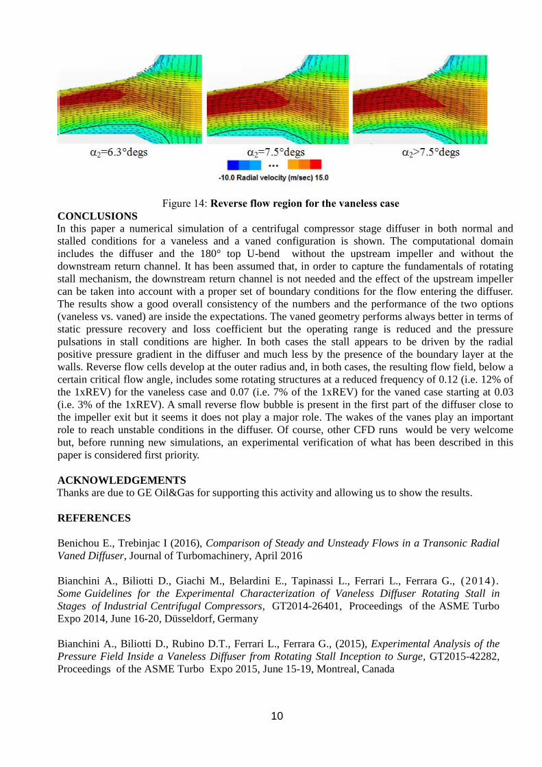
10
Figure 14: Reverse flow region for the vaneless case
CONCLUSIONS
In this paper a numerical simulation of a centrifugal compressor stage diffuser in both normal and
stalled conditions for a vaneless and a vaned configuration is shown. The computational domain
includes the diffuser and the 180° top U-bend without the upstream impeller and without the
downstream return channel. It has been assumed that, in order to capture the fundamentals of rotating
stall mechanism, the downstream return channel is not needed and the effect of the upstream impeller
can be taken into account with a proper set of boundary conditions for the flow entering the diffuser.
The results show a good overall consistency of the numbers and the performance of the two options
(vaneless vs. vaned) are inside the expectations. The vaned geometry performs always better in terms of
static pressure recovery and loss coefficient but the operating range is reduced and the pressure
pulsations in stall conditions are higher. In both cases the stall appears to be driven by the radial
positive pressure gradient in the diffuser and much less by the presence of the boundary layer at the
walls. Reverse flow cells develop at the outer radius and, in both cases, the resulting flow field, below a
certain critical flow angle, includes some rotating structures at a reduced frequency of 0.12 (i.e. 12% of
the 1xREV) for the vaneless case and 0.07 (i.e. 7% of the 1xREV) for the vaned case starting at 0.03
(i.e. 3% of the 1xREV). A small reverse flow bubble is present in the first part of the diffuser close to
the impeller exit but it seems it does not play a major role. The wakes of the vanes play an important
role to reach unstable conditions in the diffuser. Of course, other CFD runs would be very welcome
but, before running new simulations, an experimental verification of what has been described in this
paper is considered first priority.
ACKNOWLEDGEMENTS
Thanks are due to GE Oil&Gas for supporting this activity and allowing us to show the results.
REFERENCES
Benichou E., Trebinjac I (2016), Comparison of Steady and Unsteady Flows in a Transonic Radial
Vaned Diffuser, Journal of Turbomachinery, April 2016
Bianchini A., Biliotti D., Giachi M., Belardini E., Tapinassi L., Ferrari L., Ferrara G., (2014).
Some Guidelines for the Experimental Characterization of Vaneless Diffuser Rotating Stall in
Stages of Industrial Centrifugal Compressors, GT2014-26401, Proceedings of the ASME Turbo
Expo 2014, June 16-20, Düsseldorf, Germany
Bianchini A., Biliotti D., Rubino D.T., Ferrari L., Ferrara G., (2015), Experimental Analysis of the
Pressure Field Inside a Vaneless Diffuser from Rotating Stall Inception to Surge, GT2015-42282,
Proceedings of the ASME Turbo Expo 2015, June 15-19, Montreal, Canada

11
Camatti M., Betti D., Giachi M., (1997). Vaned Diffuser Development Using Numerical and
Experimental Techniques, The International Journal of Hydrocarbon Engineering, v.2 no.3 1997, pp.
46-54
Dazin A., Coudert S., Dupont P., Caignaert G., Bois G., (2008), Rotating Instability in the Vaneless
Diffuser of a Radial Flow Pump., Journal of Thermal Science 17(4), pp. 368-374
Dazin A., Cavazzini G., Pavesi G., Dupont P., Coudert S., Ardizzon G., Caignaert G., Bois G.,
(2011), High-Speed Stereoscopic PIV Study of Rotating Instabilities in a Radial Vaneless Vaneless
Diffuser., Exp. Fluids 51, pp. 83-93
Dodds J., Vahdati M., (2015), Rotating Stall Observation in a High Speed Compressor-Part 1:
Experimental Study, Journal of Turbomachinery 137(5), 051002
Dodds J., Vahdati M., (2015), Rotating Stall Observation in a High Speed Compressor-Part II:
Numerical Study, Journal of Turbomachinery 137(5), 051003
Ferrara G., Ferrari L., Baldassarre L., (2004) Rotating Stall in Centrifugal Compressor Vaneless
Diffuser: Experimental Analysis of Geometrical parameters Influence on Phenomenon Evolution,
International Journal of Rotating Machinery, Vol. 10(6), pp. 433-442
Fulton J.W., Blair W.G., (1995) . Experience with Empirical Criteria for Rotating Stall in
Radial Vaneless Diffusers, Proceedings of the Twenty-Fourth Turbomachinery Symposium Gas
Turbine Laboratories,Texas A&M, pp.97-105
Gau C., Gu C., Wang T., Yang B., Analysis of Geometries’ Effects on Rotating stall in Vaneless
diffuser with Wavelet Neural Networks, International Journal of Rotating Machinery, Volume 2007,
pp. 1-10
Giachi M., Lombardi G., Maganzi M., (2016). Centrifugal Compressors Diffuser Rotating Stall
Deep Insight, Proceedings of 3rd
International Rotating Equipment Conference, Sept. 3-4,
Düsseldorf, Germany
Jansen W., (1964). Rotating Stall in a Radial Vaneless Diffuser, Paper No.64-FE-6, ASME
Journal of Basic Engineering, pp.750-758
Japikse D., (1996). Centrifugal Compressor Design and Performance, Concepts ETI, 1996
Ješe U., Fortes-Patella R., Dular M., (2015), Numerical Study of Pump-Turbine Instabilities Under
Pumping Mode Off-Design Conditions, AJKFluids2015-33501, Proceedings of the
ASME/JSME/KSME 2015 Joint Fluids Engineering Conference, July 26-31, Seoul, South Korea
Kinoshita Y., Senoo Y., (1985). Rotating Stall Induced in Vaneless Diffusers of Very Low
Specific Speed Centrifugal Blowers, ASME Journal of Engineering for Gas Turbines and Power,
Vol.107 April 1985, pp.514-521
Ljevar S., De Lange H.C., Van Steenhoven A.A., ( 2 0 0 6 ) Two-Dimensional Rotating Stall
Analysis in a Wide Vaneless Diffuser, ID 56420, International Journal of Rotating Machinery, Vol.
2006, pp 1-11
Lievar S., (2007), Rotating Stall in Wide Vaneless Diffusers, Phd Thesis, Eindhoven University

12
Press, 2007
Marconcini M., Bianchini A.,Checcucci M., Ferrara G., Arnone A., Ferrari L., Biliotti D., Rubino
D.T., (2016). A 3D Time-Accurate CFD Simulation of the Flow Field Inside a Vaneless Diffuser
During Rotating Stall Conditions, GT2016-57604, Proceedings of ASME Turbo Expo 2016, June
13-17, Seoul, South Korea.,
Pavesi G., Dazin A., Cavazzini G., Caignaert G., Bois G., Ardizzon G., (2011). Experimental and Numerical Investigation of Un-Forced Unsteadiness in a Vaneless Radial Diffuser, Proceedings of the 9th European Conference on Turbomachinery-fluid dynamics and thermodynamics, Turkey, 2011