CENTER FOR

MACHINE PERCEPTION

CZECH TECHNICAL

UNIVERSITY

RESEARCH

REPO

RT

ISSN

1213

-236

5Learning Efficient Linear

Predictors for Motion Estimation(Version 1.13)

Jirı Matas, Karel Zimmermann, Tomas Svoboda,Adrian Hilton1

zimmerk@cmp.felk.cvut.cz

1: Centre for Vision Speech and Signal ProcessingSchool of Electronics and Physical Sciences

University of Surrey Guildford GU2 7XH UK

CTU–CMP–2006–05

May 15, 2006

Available atftp://cmp.felk.cvut.cz/pub/cmp/articles/zimmerk/ctu-cmp-2006-05.pdf

This work has been supported by The European Commission underproject IST-004176, by The Czech Academy of Sciences under project1ET101210407 and by The STINT under project Dur IG2003-2 062

Research Reports of CMP, Czech Technical University in Prague, No. 5, 2006

Published by

Center for Machine Perception, Department of CyberneticsFaculty of Electrical Engineering, Czech Technical University

Technicka 2, 166 27 Prague 6, Czech Republicfax +420 2 2435 7385, phone +420 2 2435 7637, www: http://cmp.felk.cvut.cz

Learning Efficient Linear Predictors for MotionEstimation

Jirı Matas, Karel Zimmermann, Tomas Svoboda, Adrian Hilton1

Abstract

A novel object representation for tracking is proposed. The tracked objectis represented as a constellation of spatially localised linear predictors whichare learned on a single training image. In the learning stage, sets of pixelswhose intensities allow for optimal least square predictions of the transfor-mations are selected as a support of the linear predictor.

The approach comprises three contributions: learning object specific lin-ear predictors, explicitly dealing with the predictor precision – computationalcomplexity trade-off and selecting a view-specific set of predictors suitablefor global object motion estimate. Robustness to occlusion is achieved byRANSAC procedure.

The learned tracker is very efficient, achieving frame rate generally higherthan 30 frames per second despite the Matlab implementation.

1 IntroductionReal-time object or camera tracking requires establishing correspondence in a short-baseline pair of images followed by robust motion estimation. In real-time tracking,computation time together with the relative object-camera velocity determine the max-imum displacement for which features must be matched. Local features (corners, edges,lines) or appearance templates have both been widely used to estimate narrow baselinecorrespondences [1, 8, 12] Recently more discriminative features have been introduced toincrease robustness to changes in viewpoint, illumination and partial occlusion allowingwide-baseline matching but their are too computationally expensive for tracking applica-tions [7, 6, 10, 11].

In the paper we propose a novel object representation for tracking. The tracked objectis represented as a constellation of spatially localised linear predictors. The predictorsare learned using a set of transformed versions of a single training image. In a learningstage, sets of pixels whose intensities allow for optimal prediction of the transformationsare selected as a support of the linear predictor.

The approach comprises three contributions: learning object specific linear predictorswhich allow optimal local motion estimation; explicitly defining the trade-off betweenlinear predictor complexity (i.e. size of linear predictor support) and computational cost;and selecting an view-specific set of predictors suitable for global object motion estimate.We introduce a novel approach to learn a linear predictor from a circular region aroundthe reference point which gives the best local estimation, in the least square sense, of theobject motion for a predefined range of object velocities. Spatial localisation robust to oc-clusions is obtained from predicted reference points motions by RANSAC. The approachmakes explicit the trade-off between tracker complexity and frame-rate.

Tracking by detection [3, 5] establishes the correspondences between distinguishedregions [10, 7] detected in successive images. This approach relies on the presence ofstrong, unique features allowing robust estimation of large motions by matching acrosswide-baseline views. Detection approaches also allow automatic initialisation and re-initialisation during tracking. Methods dependent on distinguished regions are not able totrack fast, saccadic motions with acceptable accuracy due to their low frame-rate.

Displacement estimation methods achieve higher frame rates but are not able to reli-ably estimate large inter-frame motions. The methods assume that there exists a neigh-bourhood where displacement can be found directly from gradients of image intensities.The well known Kanade-Lucas tracker [8, 1] assumes that total intensity difference (dis-similarity) is a convex function in some neighbourhood. Thus, the motion is estimated bya few iterations of the Newton-Raphson method, where the difference image is multipliedby the pseudo-inverse of the image gradient. This idea was extended by Cootes [2] and ap-plied to tracking by Jurie et al. [4, 9] who learn a linear approximation of the relationshipbetween the local dissimilarity image and displacement. Online tracking is performed bymultiplying the difference image by a matrix representing the linear function. This is com-putationally efficient because no gradient or pseudo-inversion are required. Recently thisapproach [13] has been extended to more general regression functions, where displace-ments are estimated by RVM. Such methods can learn a larger range of pose changes buttracking is more complex resulting in a lower frame-rate.

The computation cost of tracking is a trade-off between the time required for dis-placement estimation and the distance moved between successive frames. Therefore, wepropose a tracking method which explicitly models the trade-off between tracker com-plexity and frame-rate. Given the expected maximum velocity of the object we learn theoptimal support of linear predictors for frame-rate tracking.

It is desirable to have efficient tracking and motion estimation to limit the object move-ment between successive estimates. In this paper, we extend the computationally efficienttracking using linear models of motion proposed by Jurie et al. [4], whose linear predic-tors use a support around pixels with high gradient values. Instead, our approach learnsthe support suitable for estimation of the linear motion model. Given a circular regionaround a reference point we learn the k best pixels to estimate the linear motion fromsynthesised training images with known motion giving the optimal linear predictor sup-port. Selection of predictors, suitable for the global object motion is performed online.This approach tracks a view-specific set of reference points using the optimal supports forefficient tracking with a known relationship between maximum object-camera velocity,motion estimation accuracy and computation time.

The rest of the paper is organised as follows. Section 2 introduces learning of linearpredictors templates and reference points set, respectively. Section 3 describes trackingand the optimal size of the template neighbourhood. Following Section 4 shows the ex-periments and the last Section 5 summarises the results and conclusions.

2 Motion EstimationIn this section we introduce a method for learning a linear predictor as well as a subset ofa given size from a circular region around the reference point, which minimise a trainingerror. This subset is called a linear predictor support and the size is called complexity of

Region

Reference point

Object

Linear predictor support

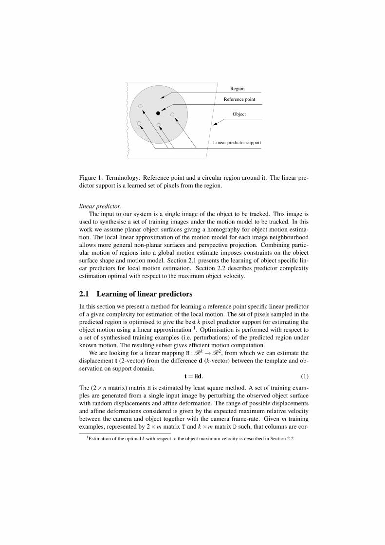
Figure 1: Terminology: Reference point and a circular region around it. The linear pre-dictor support is a learned set of pixels from the region.

linear predictor.The input to our system is a single image of the object to be tracked. This image is

used to synthesise a set of training images under the motion model to be tracked. In thiswork we assume planar object surfaces giving a homography for object motion estima-tion. The local linear approximation of the motion model for each image neighbourhoodallows more general non-planar surfaces and perspective projection. Combining partic-ular motion of regions into a global motion estimate imposes constraints on the objectsurface shape and motion model. Section 2.1 presents the learning of object specific lin-ear predictors for local motion estimation. Section 2.2 describes predictor complexityestimation optimal with respect to the maximum object velocity.

2.1 Learning of linear predictorsIn this section we present a method for learning a reference point specific linear predictorof a given complexity for estimation of the local motion. The set of pixels sampled in thepredicted region is optimised to give the best k pixel predictor support for estimating theobject motion using a linear approximation 1. Optimisation is performed with respect toa set of synthesised training examples (i.e. perturbations) of the predicted region underknown motion. The resulting subset gives efficient motion computation.

We are looking for a linear mapping H : Rk → R2, from which we can estimate thedisplacement t (2-vector) from the difference d (k-vector) between the template and ob-servation on support domain.

t = Hd. (1)

The (2×n matrix) matrix H is estimated by least square method. A set of training exam-ples are generated from a single input image by perturbing the observed object surfacewith random displacements and affine deformation. The range of possible displacementsand affine deformations considered is given by the expected maximum relative velocitybetween the camera and object together with the camera frame-rate. Given m trainingexamples, represented by 2×m matrix T and k×m matrix D such, that columns are cor-

1Estimation of the optimal k with respect to the object maximum velocity is described in Section 2.2

responding pairs of displacements and intensity differences, the least-squares solution is:

H = TD+ = TD>(DD>)−1 (2)

Supporting set need not include all the pixels from a predicted region. For example inuniform image areas pixels will add no additional information to the transformation es-timation whereas pixels representing distinct features (edges, corners, texture) will beimportant for localisation. We therefore want to select the subset of k pixels for a pre-dicted region which provides the best local estimate of the motion according to the linearmodel defined in equation 1. The quality of a given subset of the pixels can be measuredby the error of the transform estimated on the training data:

e = ‖HD−T‖F (3)

For k pixels from the radius s we have(

πs2

k

)possible subsets of pixels. Explicit evalua-

tion of the training error for all possible subsets is prohibitively expensive, we thereforeestimate an optimal subset by randomised sampling.

The above analysis considers a single linear function H approximating the relationshipbetween the observed image difference and object motion for a predicted region. Thisallows motion estimation upto a known approximation error. For a given region of radiusR the linear model gives an approximation error r << R such that 95% of the estimatedmotions are within r of the known true value. Typically in this work R ≈ 20− 30 pixelsand the resulting r ≈ 2− 5 pixels for a planar homography. Given a set of local motionestimates for different regions a robust estimate of the global object motion is obtainedusing RANSAC to eliminate the remaining 5% of outliers Section 3.

To increase the range across which we can reliably estimate the object motion wecan approximate the non-linear relationship between image displacement and motion bya piece-wise linear approximation of increasing accuracy. For a given region we learn aseries of linear functions H0, . . . ,Hq giving successive 95% approximation errors r0, . . . ,rqwhere r0 > r1 > .. . > rq. This increases the maximum object velocity without a significantincrease in computational cost.

2.2 Learning of predictor complexityIn this section we analyse the performance of the motion estimation algorithm versusframe-rate. To achieve real-time tracking we generally want to utilise the observationsat each frame to obtain a new estimate of the motion. This requires a trade-off betweentracking complexity and estimation error due to object motion. Here we assume a maxi-mum object velocity and optimise the motion estimation for tracking at frame-rate.

For a single linear predictor the error of displacement estimation decreases with re-spect to its complexity (i.e. the number of pixels k selected from the predicted region).However, as k increases the error converges to a constant value with decreasing negativegradient. The error will only decrease when new structural information about the localvariation in surface appearance is added. In uniform regions the variation is due to imagenoise and will not decrease localisation error. The computation cost increases linearlywith the number of pixels used, k. Therefore, we seek to define an optimal trade-offbetween computation time and motion estimation error.

Since the time needed for displacement estimation is a linear function of the numberof pixels t = ak, the displacement error e(t) is also a decreasing function of time. During

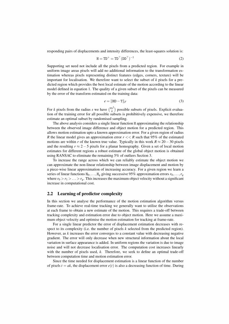
Figure 2: Distance d(t) from the real position of the object and its minimum.

the displacement estimation, the object moves away from the observation. The distanced(t) from the real position of the object in the worst case is

dmax(t) = e(t)+ vmaxt, (4)

where vmax is the maximum velocity of the object in pixels. Figure 2 shows the char-acteristic of the maximum distance and the motion estimation error e(t) with increasingnumber of pixels k or time.

Assuming e(t) = de(t)dt is a monotonically decreasing function, Equation 4 has a unique

solution given by:t∗ = argmin

t(d(t)) = e−1(−vmax) (5)

The complexity of the tracker which minimises motion estimation error for real-time trac-ing is k∗ = t∗

a . The worst expected accuracy error is e(t∗)+ vmaxt∗. Similarly, given therequired accuracy, the maximum speed of the object could be estimated.

3 TrackingMotion estimation for each individual prediction support requires a single matrix multi-plication using Equation 1. The cost of this operation is proportional to the number k ofpixels in the regions. Matrix H is estimated offline in a pre-processing stage using thesynthesised training examples. Iterative refinement of the linear approximation using ahierarchy of q linear approximations H0, ...,Hq requires O(pkq) operations, where p is thenumber of regions and k is the predictor complexity.

Global motion estimation for a set of p regions is estimated using RANSAC to pro-vide robustness to errors in local motion estimates and partial occlusion. In this workwe assume planar object surfaces giving image motion defined by a homography with

eight degrees-of-freedom. Once the motion of each region is estimated, we use 4-pointRANSAC to filter out outliers and compute the correct motion of the object. Note, thatthis homography is applied to both the reference point positions and the supporting sets.

3.1 Active region setRobust motion estimation in the presence of occlusion requires regions to be distributedacross the object surface. It is not possible to find the set of regions suitable for objecttracking independently on the object position, because if the object gets closer to thecamera some regions can disappear and the global motion estimation can easily becomeill-conditioned. In this section we present an online method which automatically selectsthe p-regions subset, called active region set, from all visible regions which provide themost accurate motion estimate and is sufficiently robust.

To optimise the distribution of regions across the surface, we define a coverage mea-sure of the region set X ,

c(X) = ∑x∈X

d(x,X \x), (6)

where distance between point x and set X is defined as the distance from the closestelement of the set

d(x,X) = miny∈X

‖x−y‖. (7)

Ideally for optimal robustness to occlusion the coverage measure would be max-imised. In practice, individual regions have an associated localisation error which mustbe taken into account. The quality q(x) of individual regions is measured by their meanerror e(x) on the training data.

q(x) = maxy∈X

(e(y)

)− e(x). (8)

To find a suitable subset X of regions from all visible regions X we seek to optimise theweighted combination of the coverage and quality:

f (X) = wc(X)c(X)

+(1−w)q(X)q(X)

, (9)

where w ∈ [0;1] is the coverage weight. Given the maximum number of regions p wesearch for the optimal set of regions using the greedy search strategy presented in Algo-rithm 1.

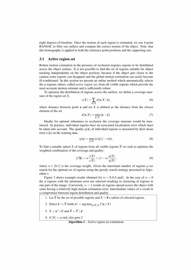
Figure 3 shows example results obtained for w = 0,0.5,and1. In the case of w = 0the p regions with the minimum error are selected resulting in clustering of regions inone part of the image. Conversely, w = 1 results in regions spread across the object withsome having a relatively high motion estimation error. Intermediate values of w result ina compromise between region distribution and quality.

1. Let X be the set of possible regions and X = /0 a subset of selected regions.

2. Select x∗ ∈ X holds x∗ = argmaxx∈X\X f (x∪X)

3. X = x∗∪X and X = X \x∗

4. if |X |= p end, else goto 2Algorithm 1 - Active region set estimation.

4 ExperimentsThe proposed method was tested on several different sequences of planar objects. Wedemostrate robustness to large scaling and strong occlusions as well as saccadic motions(e.g. like shaking), where object motion is faster than 30 pixels per frame. Section 4.1investigates region suitability and influence of the coverage weight. We show that eventhe regions which are strong features, in the sense of Shi and Kanade [12] definition, maynot be suitable for tracking. Section 4.2 summaries advantages and drawbacks of methodsfor linear predictor support estimation and Section 4.3 shows real experiments and discussvery low time complexity.

4.1 Active region set estimation

Figure 3: Object coverage by regions for w = 0,0.5,1. Blue circles correspond to the allpossible regions, red crosses to the selected regions. Size of crosses corresponds to thetraining error.

In this experiment, we show influence of coverage weight on active region set anddiscuss region suitability for tracking. Different region sets selected for different weightsare shown at Figure 3. The set of all possible regions is depicted by blue circles. Activeregion set of the most suitable 17 regions is labeled by red crosses, where size of thecross corresponds to the training error of the particular region. The weight defines thecompromise between coverage and quality of the regions. The higher is the weight, themore uniform is the object coverage.

In the last case (w = 1), we can see that the teeth provide very high tracking error,although they are one of the strongest features due to the high values of gradient in theirneighbourhood. The repetitive structure of teeth causes that different displacements cor-respond to the almost same observations. If the range of displacement had been smallerthan teeth period, the training error would have been probably significantly smaller. Inthis sense, region quality is depends on the expected object velocity (or machine perfor-mance).

4.2 Comparison of different methods for linear predictor supportestimation

In this experiment we compare several different methods for linear predictor support se-lection. The experiment was conducted on approximately 100 regions. From each regionof 30-pixel radius a subset of 63 pixels was selected supporting by different methods.

Figure 4: Comparison of different methods for linear predictor support estimation.

Figure 4.2 compares average errors of tracking on artificial testing examples for dif-ferent ranges of displacements of the following methods:

• Equally distributed pixels over the region - the support consists of pixels lying on aregular grid.

• Equally distributed with gradient based selection - pixels are divided into the grid-bins. The pixels with the highest gradient from each bin forms the support.

• Normal re-projection - First the least square solution is found for the whole n-pixel region. Each row of the obtained matrix H corresponds to the normal vectorof n-dimensional hyper-plane. Particular components provide an information aboutpixel significance. The pixels corresponding to the highest components are utilised.

• Randomised sampling - Random subsets are repetitively selected from the region.Those which provide the lowest training error are utilised..

Since the global minimum estimation is for reasonable regions simply intractable, itis necessary to use a heuristic method. Randomized sampling seems as the best choice,because even as few as 20 iterations provide very good results. The more iterations isperformed, the closer to the global minimum we can get. In the other hand, randomisedsampling requires as many estimation of least square problem as iterations. If someonelooks for a fast heuristic (e.g. for online learning) then normal re-projection method is anatural compromise.

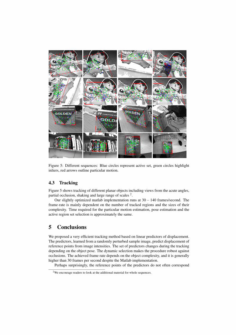
Figure 5: Different sequences: Blue circles represent active set, green circles highlightinliers, red arrows outline particular motion.

4.3 TrackingFigure 5 shows tracking of different planar objects including views from the acute angles,partial occlusion, shaking and large range of scales 2.

Our slightly optimized matlab implementation runs at 30− 140 frames/second. Theframe-rate is mainly dependent on the number of tracked regions and the sizes of theircomplexity. Time required for the particular motion estimation, pose estimation and theactive region set selection is approximately the same.

5 ConclusionsWe proposed a very efficient tracking method based on linear predictors of displacement.The predictors, learned from a randomly perturbed sample image, predict displacement ofreference points from image intensities. The set of predictors changes during the trackingdepending on the object pose. The dynamic selection makes the procedure robust againstocclusions. The achieved frame rate depends on the object complexity, and it is generallyhigher than 30 frames per second despite the Matlab implementation.

Perhaps surprisingly, the reference points of the predictors do not often correspond

2We encourage readers to look at the additional material for whole sequences.

to classical feature points which are mostly anchored at points with high gradient. Thestrength of method lies in the learning stage. The predictors are learned from the expectedmaximum velocity. The predictors are linear but strong enough to cover wide range ofmotions. The linearity allows for efficient learning.

References[1] S. Baker and I. Matthews. Lucas-kanade 20 years on: A unifying framework. Inter-

national Journal of Computer Vision, 56(3):221–255, 2004.

[2] T.F. Cootes, G.J. Edwards, and C.J. Taylor. Active appearance models. PAMI,23(6):681–685, June 2001.

[3] I. Gordon and D.G. Lowe. Scene modelling, recognition and tracking with invari-ant image features. In International Symposium on Mixed and Augmented Reality(ISMAR), pages 110–119, 2004.

[4] F. Jurie and M. Dhome. Real time robust template matching. In British MachineVision Conference, pages 123–131, 2002.

[5] V. Lepetit, P. Lagger, and P. Fua. Randomized trees for real-time keypoint recogni-tion. In Computer Vision and Pattern Recognition, pages 775–781, 2005.

[6] D. Lowe. Distinctive image features from scale-invariant keypoints. IJCV, 60(2),2004. 91-110.

[7] D.G. Lowe. Object recognition from local scale-invariant features. In InternationalConference on Computer Vision, pages 1150–1157, 1999.

[8] B.D. Lucas and T. Kanade. An iterative image registration technique with an appli-cation to stereo vision. In IJCAI, pages 674–679, 1981.

[9] L. Masson, M. Dhome, and F. Jurie. Robust real time tracking of 3d objects. InInternational Conference on Pattern Recognition, 2004.

[10] J. Matas, O. Chum, M. Urban, and T. Pajdla. Robust wide-baseline stereo frommaximally stable extremal regions. Image and Vision Computing, 22(10):761–767,September 2004.

[11] K. Mikolajczyk, T. Tuytelaars, C. Schmid, A. Zisserman, J. Matas, F. Schaffalitzky,T. Kadir, and L. van Gool. A comparison of affine region detectors. IJCV, 65(7):43–72, 2005.

[12] Jianbo Shi and Carlo Tomasi. Good features to track. In Computer Vision andPattern Recognition (CVPR’94), pages 593 – 600, 1994.

[13] O. Williams, A. Blake, and R. Cipolla. Sparse bayesian learning for efficient visualtracking. Pattern Analysis and Machine Intelligence, 27(8):1292–1304, 2005.