ccc.illinois.educcc.illinois.edu/s/Reports14/Secondary Cooling and Control... · DISTRIBUTED...

DISTRIBUTED PARAMETER CONTROL OF HEAT DIFFUSION WITHSOLIDIFICATION

BY

BRYAN PETRUS

DISSERTATION

Submitted in partial fulfillment of the requirementsfor the degree of Doctor of Philosophy in Mechanical Engineering

in the Graduate College of theUniversity of Illinois at Urbana-Champaign, 2014

Urbana, Illinois

Doctoral Committee:

Professor Joseph Bentsman, ChairProfessor Brian G. Thomas, Co-ChairProfessor Naira HovakimyanProfessor Tamer Basar

ABSTRACT

Continuous casting is an important engineering process which produces nearly all steel cur-

rently used worldwide. Regulation of the temperature of the steel during casting with water

sprays is known to be important to final product quality and safely operating the caster. Yet

most current control methods are effectively open-loop, due to the complicated nature of the

process. Measurements of the steel temperature cannot be made reliably due to the high

temperatures and constant water spray in the caster. Even if feedback could be obtained,

the temperature of the steel is governed by a nonlinear partial differential equation (PDE),

which presents a challenge for existing control techniques.

In the first part of this dissertation, the state-of-the art in industrial control systems

for this process is described. The primary difficulty this system deals with is the sensing

problem. Instead of physical sensors, a real-time computational model of the caster is

used as a “software sensor.” Using the model for feedback, a simple proportional integral

(PI) controller bank is able to adequately regulate the surface temperature. Using multiple

independent 1-D models interpolated to provide a 2-D prediction of the steel temperature,

the model is able to run in real-time even at the high casting speeds of a thin-slab steel caster.

The model is calibrated through steady state measurements of the thin-slab caster from

reliable pyrometer measurements outside the spray zone and metallurgical length detection

trials. The use of independent 1-D models is verified by comparing model predictions with

transient measurements of roll forces in another caster. The model is further used to perform

a computational study of the temperature and shell thickness in a caster during sudden speed

changes.

In the second part, the control problem is studied for a simpler, but still fundamentally

nonlinear PDE model of the caster. Using Lyapunov stability theory for infinite-dimensional

ii

systems, a control law is designed that matches the entire distributed temperature of a 1-D

slice through control of the heat flux at the steel surface. In the first version, the control law

is based on only examining the temperature error, and produces a control law with sharply

varying and unbounded heat flux. In the second version, a control law that performs much

better is found by considering the error in enthalpy for feedback. The second control design

is also proven to work for models better approximating the real system, in particular limits

on the heat flux due to the spray water piping system design.

In the final part, the control law designed in the second part is simulated on a model

including some of the most important difficulties of the real system, namely non-symmetric

boundary conditions and actuator saturation, and performs admirably. The controller still

uses a software sensor, as in the first part, so the uncertainty of the model is quantitatively

examined. Finally, some additional unproven conjectures are offered that are based on

simulation evidence. In particular, a boundary sensing solution is proposed that is not yet

proved, but works well in simulation.

iii

To my parents, Jim and Karen Petrus, for everything.

iv

ACKNOWLEDGMENTS

To paraphrase John Donne, no grad student is an island; ask not by whom the dissertation

is written, it was written with the help of a lot of people. In my research and writing, I

have borrowed ideas and hard work from numerous others whose names are not on the front

page. I have tried to thank as many as I could below, but the list is by no means complete.

I apologize to the many whose names I forgot to include.

Professor Joseph Bentsman is the reason I fell in love with the field of control systems. If

I can keep a small fraction of the enthusiasm and knowledge he has for the subject, I will

count myself very lucky.

I am very grateful for the opportunity to work in the Continuous Casting Consortium,

created and run by Professor Brian G. Thomas. The consortium exemplifies two qualities

of its founder: excitement for the making of steel, and the belief that great engineering

research is not isolated to academic labs but can be accomplished by working hand in hand

with industry.

I have often told incoming graduate students that the single greatest part of graduate

school was the ability to listen to some of the greatest minds in your field teach classes

about their favorite subjects and new research. When I said this, I was specifically thinking

of the classes I have taken from Professors Naira Hovakimyan and Tamer Basar. I was

indebted to them before they agreed to serve on my committee, and am only more grateful

now.

Kai Zheng, formerly of the University of Illinois and now of ArcelorMittal Global R&D,

did the original design and programming of the Cononline system.

Xiaoxu Zhou, formerly of the University of Illinois and currently of SSAB Americas R&D,

calibrated CON1D to the Nucor Decatur steel mill, and worked on the CON1D code

v

that is part of Cononline. This calibration was aided by Sami Vapalahti, formerly Helsinki

University of Technology, and also by Roger Yang during his undergrad research at the

University of Illinois.

Prathiba Duvuuri, of the University of Illinois, performed empirical investigations into

mold heat flux, and numerical investigations into spray cooling, for the Nucor Decatur Steel

Mill as part of the work in this dissertation.

Rob Oldroyd, currently of Nucor, wrote the TCP/IP and shared memory code in Conon-

line, and the initial version of CononlineMonitor.

Kris Sledge and Terri Morris of Nucor were the primary forces in implementation and

integration of Cononline with Nucor automation. They also guided all work discussed here

that involved the plant database at Nucor Decatur.

This work would not have been possible without the contributions of many plant operators,

metallurgists, engineers, and supervisors at Nucor Decatur to testing and improvements of

the Cononline system. With sincere apologies to the many important names not on this list,

those include: Steve Dunnavant, Caster Green, Danny Hammond, Mike Langley, Megan

Miller, Ron O’Malley, Rodney Thrasher, Wes Wadell, and Bob Williams.

Rudolf Moravec and Ken Blazek of ArcelorMittal Global R&D graciously provided some

additional information on the trials at Burns Harbor that allowed more accurate simulations

of the trials.

The numerical simulations performed in Part II are based off of code originally written

by Vivek Natarajan, formerly of the University of Illinois and currently of the University of

Tel Aviv.

Lance Hibbeler graciously guided the uncertainty analysis of CON1D.

This work has been funded in part by two NSF grants, DMI-0500453 and CMMI-0900138.

My heartfelt thanks to the sponsors of the Continuous Casting Consortium, both in par-

ticular for funding this research, and in general for funding a group where I have been able

to watch researchers at a major research university work with the best operators, engineers,

and metallurgists in the industry.

Thank you to the many students of the Control Systems Design and Applications Lab,

and the Material Process Modelling Lab, for their occasional help, and continuing friendship.

vi

I want to especially thank all of the staff of the Department of Mechanical Science and En-

gineering at the University of Illinois, including Kathy Smith, Kara Breyer, Debbie Richard-

son, Pam Vanetta, and others who helped during some of the most stressful times in my

life.

vii

TABLE OF CONTENTS

LIST OF TABLES . . . . . . . . . . . . . . . . . . . . . . . . . . . . . . . . . . . . . x

LIST OF FIGURES . . . . . . . . . . . . . . . . . . . . . . . . . . . . . . . . . . . . xi

LIST OF ABBREVIATIONS . . . . . . . . . . . . . . . . . . . . . . . . . . . . . . . xv

LIST OF SYMBOLS . . . . . . . . . . . . . . . . . . . . . . . . . . . . . . . . . . . . xvi

CHAPTER 1 INTRODUCTION . . . . . . . . . . . . . . . . . . . . . . . . . . . . 11.1 Motivating application . . . . . . . . . . . . . . . . . . . . . . . . . . . . . . 11.2 Literature review . . . . . . . . . . . . . . . . . . . . . . . . . . . . . . . . . 31.3 Overview . . . . . . . . . . . . . . . . . . . . . . . . . . . . . . . . . . . . . . 61.4 Process model . . . . . . . . . . . . . . . . . . . . . . . . . . . . . . . . . . . 7

I State-of-the-art industrial model and control for steel contin-uous casters . . . . . . . . . . . . . . . . . . . . . . . . . . . . . 11

CHAPTER 2 STATE-OF-THE-ART INDUSTRIAL CONTROL METHOD: CONON-LINE . . . . . . . . . . . . . . . . . . . . . . . . . . . . . . . . . . . . . . . . . . . 122.1 Introduction . . . . . . . . . . . . . . . . . . . . . . . . . . . . . . . . . . . . 122.2 Control system overview . . . . . . . . . . . . . . . . . . . . . . . . . . . . . 132.3 System Architecture and Implementation . . . . . . . . . . . . . . . . . . . . 152.4 System Components . . . . . . . . . . . . . . . . . . . . . . . . . . . . . . . 172.5 Additional control problems and solutions . . . . . . . . . . . . . . . . . . . 37

CHAPTER 3 VALIDATION OF CONSENSOR MODEL . . . . . . . . . . . . . . . 443.1 Steady-state validation of CON1D at Nucor Decatur . . . . . . . . . . . . . 443.2 Transient validation with Burns Harbor results . . . . . . . . . . . . . . . . . 50

CHAPTER 4 SIMULATION CASE STUDIES FOR THIN-SLAB CASTER . . . . 604.1 Casting conditions . . . . . . . . . . . . . . . . . . . . . . . . . . . . . . . . 604.2 Constant secondary cooling (no spray control) . . . . . . . . . . . . . . . . . 614.3 Sequential speed changes, and effect of control strategy . . . . . . . . . . . . 74

viii

II Developing a control theory for nonlinear PDEs describingsolidification . . . . . . . . . . . . . . . . . . . . . . . . . . . . . 82

CHAPTER 5 CONTROL LAW FROM TEMPERATURE-BASED LYAPUNOVFUNCTIONAL . . . . . . . . . . . . . . . . . . . . . . . . . . . . . . . . . . . . . 835.1 The two–phase Stefan Problem . . . . . . . . . . . . . . . . . . . . . . . . . 845.2 Control law . . . . . . . . . . . . . . . . . . . . . . . . . . . . . . . . . . . . 865.3 Simulation results . . . . . . . . . . . . . . . . . . . . . . . . . . . . . . . . . 925.4 Summary . . . . . . . . . . . . . . . . . . . . . . . . . . . . . . . . . . . . . 94

CHAPTER 6 CONTROL LAW FROM ENTHALPY-BASED LYAPUNOV DESIGN 996.1 Modeling simplification: the one-phase Stefan problem . . . . . . . . . . . . 996.2 Preliminaries and notation . . . . . . . . . . . . . . . . . . . . . . . . . . . . 1006.3 Control law . . . . . . . . . . . . . . . . . . . . . . . . . . . . . . . . . . . . 1026.4 Discussion and Simulation Results . . . . . . . . . . . . . . . . . . . . . . . . 1046.5 Summary . . . . . . . . . . . . . . . . . . . . . . . . . . . . . . . . . . . . . 108

CHAPTER 7 EXTENSIONS FOR BETTER MODEL FIDELITY . . . . . . . . . . 1107.1 The two–sided Stefan Problem . . . . . . . . . . . . . . . . . . . . . . . . . . 1107.2 Input saturation . . . . . . . . . . . . . . . . . . . . . . . . . . . . . . . . . . 1137.3 Summary . . . . . . . . . . . . . . . . . . . . . . . . . . . . . . . . . . . . . 120

III Synthesis and future work . . . . . . . . . . . . . . . . . . 122

CHAPTER 8 LOOP CLOSURE ISSUES AND UNCERTAINTY ANALYSIS . . . . 1238.1 Applicability of assumptions to steel casting . . . . . . . . . . . . . . . . . . 1238.2 Quantitative uncertainty analysis of the estimator . . . . . . . . . . . . . . . 1278.3 Use of sparse measurements for re-calibration . . . . . . . . . . . . . . . . . 133

CHAPTER 9 CONJECTURES, SUGGESTIONS FOR FUTURE WORK, ANDCONCLUSIONS . . . . . . . . . . . . . . . . . . . . . . . . . . . . . . . . . . . . 1419.1 Conjectures . . . . . . . . . . . . . . . . . . . . . . . . . . . . . . . . . . . . 1419.2 Future work . . . . . . . . . . . . . . . . . . . . . . . . . . . . . . . . . . . . 1469.3 Conclusions . . . . . . . . . . . . . . . . . . . . . . . . . . . . . . . . . . . . 148

APPENDIX A NUMERICAL SIMULATION BACKGROUND . . . . . . . . . . . . 149

APPENDIX B MATH BACKGROUND . . . . . . . . . . . . . . . . . . . . . . . . 152B.1 Lyapunov stability and LaSalle invariance . . . . . . . . . . . . . . . . . . . 152B.2 Infinite–dimensional systems . . . . . . . . . . . . . . . . . . . . . . . . . . . 153B.3 Useful inequalities and estimates . . . . . . . . . . . . . . . . . . . . . . . . . 156

REFERENCES . . . . . . . . . . . . . . . . . . . . . . . . . . . . . . . . . . . . . . . 157

ix

LIST OF TABLES

2.1 Separate software programs in Cononline control system . . . . . . . . . . . 152.2 Controller assignments. . . . . . . . . . . . . . . . . . . . . . . . . . . . . . . 352.3 Controller gains . . . . . . . . . . . . . . . . . . . . . . . . . . . . . . . . . . 36

4.1 Results of linear regression on metallurgical length data in Figure 4.6 . . . . 654.2 Calculation of k-factor for steady-state MLs predicted by Consensor. . . . . . 68

5.1 Thermodynamic properties used in section 5.3 . . . . . . . . . . . . . . . . . 93

6.1 Thermodynamic properties used in section 6. . . . . . . . . . . . . . . . . . . 105

8.1 Assumed uncertainties in calibration of computational model / estimatorof thin-slab caster. . . . . . . . . . . . . . . . . . . . . . . . . . . . . . . . . 132

8.2 Assumed uncertainties in measurements input to computational model /estimator of thin-slab caster. . . . . . . . . . . . . . . . . . . . . . . . . . . . 133

x

LIST OF FIGURES

1.1 Schematic diagram of continuous steel caster (B.G. Thomas and L.C. Hibbeler) 2

2.1 Overview of Cononline control system with software sensor, Consensor,and PI controller, Concontroller. . . . . . . . . . . . . . . . . . . . . . . . . . 14

2.2 Cononline system architecture. . . . . . . . . . . . . . . . . . . . . . . . . . . 162.3 Closed loop block diagram with Consensor predictor and Concontroller PI

controller bank. . . . . . . . . . . . . . . . . . . . . . . . . . . . . . . . . . . 202.4 Thermodynamic properties of 0.05 wt-% Carbon steel, using the referenced

microsegregation and material property models. . . . . . . . . . . . . . . . . 222.5 Comparison of Cononline predicted mold heat flux with measurements. . . . 242.6 Illustration of heat transfer coefficients in spray zone. . . . . . . . . . . . . . 252.7 Illustration of Consensor simulation domain. . . . . . . . . . . . . . . . . . . 272.8 Illustration of Consensor delay interpolation technique. . . . . . . . . . . . . 292.9 Linear interpolation of slice surface temperatures, with 200 slices in 15 m

long Nucor Decatur caster. . . . . . . . . . . . . . . . . . . . . . . . . . . . . 302.10 Illustration of transient estimation error due to Consensor delay interpo-

lation technique. . . . . . . . . . . . . . . . . . . . . . . . . . . . . . . . . . 322.11 Diagram of spray zones in the Nucor Decatur casters. . . . . . . . . . . . . . 342.12 Screen shots of CononlineMonitor during casting. . . . . . . . . . . . . . . . 38

3.1 Pyrometer installation in the Nucor Decatur south caster. . . . . . . . . . . 453.2 Comparison of CON1D surface temperature predictions with measure-

ments from optical pyrometers. . . . . . . . . . . . . . . . . . . . . . . . . . 463.3 Schematic illustration of sensor-less metallurgical length detection. . . . . . . 483.4 Data collected during performance of metallurgical length detection trial

at Nucor Decatur. . . . . . . . . . . . . . . . . . . . . . . . . . . . . . . . . . 493.5 Predictions of dynamic temperature, solidification, and thermal shrinkage

model during series of speed change in Burns Harbor caster, compared tomeasured roll loads. . . . . . . . . . . . . . . . . . . . . . . . . . . . . . . . . 52

3.6 Temperature, solid fraction, and TLE profile through transverse slice ofthe strand at several points in the caster, traveling at constant 1.1 m/mincasting speed. . . . . . . . . . . . . . . . . . . . . . . . . . . . . . . . . . . . 54

3.7 Inner radius surface temperature, shell thickness, and average TLE of aslice of the strand as it travels through the caster at steady 1.1 m/mincasting speed. . . . . . . . . . . . . . . . . . . . . . . . . . . . . . . . . . . . 54

xi

3.8 Illustration of method for calculating dynamic TLE in Consensor. . . . . . . 57

4.1 Illustration of “spray-table” of speed-based water flow rates used in NucorDecatur secondary cooling zone. . . . . . . . . . . . . . . . . . . . . . . . . . 61

4.2 Model prediction of thin-slab caster during sudden 0.5 m/min speed drop. . 624.3 Model prediction of thin-slab caster during sudden 1 m/min speed drop. . . 634.4 Model prediction of thin-slab caster during sudden 2 m/min speed drop. . . 634.5 Model prediction of thin-slab caster during sudden 3 m/min speed drop. . . 644.6 Metallurgical length during sudden speed drops. . . . . . . . . . . . . . . . . 654.7 Illustration of liquid pool being pinched off during sudden speed drop from

3.5 to 0.5 m/min . . . . . . . . . . . . . . . . . . . . . . . . . . . . . . . . . 664.8 Model prediction of thin-slab caster during sudden 0.25 m/min speed increase. 694.9 Model prediction of thin-slab caster during sudden 0.5 m/min speed increase. 704.10 Model prediction of thin-slab caster during sudden 1 m/min speed increase. . 704.11 Model prediction of thin-slab caster during sudden 2 m/min speed increase. . 714.12 Settling times for surface temperature in bender, straightener, and final

segment showing calculated values from simulations and estimated valuesusing equation (4.9). . . . . . . . . . . . . . . . . . . . . . . . . . . . . . . . 72

4.13 Metallurgical length during sudden speed increases. . . . . . . . . . . . . . . 734.14 Settling times for metallurgical length calculated from simulations. . . . . . . 744.15 Model prediction of thin-slab caster during sequential sudden 1 m/min

slow-down and speed-up, with 5 minutes in between speed changes, withconstant spray cooling. . . . . . . . . . . . . . . . . . . . . . . . . . . . . . . 75

4.16 Model prediction of thin-slab caster during sequential sudden 1 m/minslow-down and speed-up, with 4 minutes in between speed changes, withconstant spray cooling. . . . . . . . . . . . . . . . . . . . . . . . . . . . . . . 76



4.19 Model prediction of thin-slab caster during sequential sudden 1 m/minslow-down and speed-up, with 1 minute in between speed changes, withconstant spray cooling. . . . . . . . . . . . . . . . . . . . . . . . . . . . . . . 77

4.20 Model prediction of thin-slab caster during sequential sudden 1 m/minslow-down and speed-up, with 5 minutes in between speed changes, withspeed-based spray cooling control. . . . . . . . . . . . . . . . . . . . . . . . . 79

4.21 Model prediction of thin-slab caster during sequential sudden 1 m/minslow-down and speed-up, with 1 minute in between speed changes, withspeed-based spray cooling control. . . . . . . . . . . . . . . . . . . . . . . . . 79

4.22 Model prediction of thin-slab caster during sequential sudden 1 m/minslow-down and speed-up, with 5 minutes in between speed changes, withtemperature-based PI spray cooling control. . . . . . . . . . . . . . . . . . . 80

xii

4.23 Model prediction of thin-slab caster during sequential sudden 1 m/minslow-down and speed-up, with 1 minute in between speed changes, withtemperature-based PI spray cooling control. . . . . . . . . . . . . . . . . . . 80

5.1 Simplified block diagram . . . . . . . . . . . . . . . . . . . . . . . . . . . . . 845.2 Initial condition for simulations in Section 5 . . . . . . . . . . . . . . . . . . 935.3 Simulation of system (1.7)-(1.10) with initial condition mismatch and no

control adjustment . . . . . . . . . . . . . . . . . . . . . . . . . . . . . . . . 955.4 Simulation of system (1.7)-(1.10) with initial condition mismatch and con-

trol law (5.5) . . . . . . . . . . . . . . . . . . . . . . . . . . . . . . . . . . . 965.5 Simulation of system (1.7)-(1.10) with initial condition mismatch and con-

trol law (5.12) . . . . . . . . . . . . . . . . . . . . . . . . . . . . . . . . . . . 975.6 Overview block diagram for Chapter 5. . . . . . . . . . . . . . . . . . . . . . 985.7 Block diagram showing equations from Chapter 5. . . . . . . . . . . . . . . . 98

6.1 Initial condition for simulations in Chapter 6 . . . . . . . . . . . . . . . . . . 1066.2 Simulation of system (1.7)-(1.10) with initial condition mismatch and con-

trol law (6.6) . . . . . . . . . . . . . . . . . . . . . . . . . . . . . . . . . . . 1076.3 Overview block diagram for Chapter 6. . . . . . . . . . . . . . . . . . . . . . 1096.4 Block diagram showing equations from Chapter 6. . . . . . . . . . . . . . . . 109

7.1 Initial condition for simulations in Section 7.1.2. . . . . . . . . . . . . . . . . 1147.2 Temperature error T for two-sided Stefan Problem (7.1)-(7.4), with initial

conditions from Figure 7.1 and Neumann boundary control (7.10). . . . . . . 1157.3 Temperature error T for two-sided Stefan Problem (7.1)-(7.4), with initial

conditions from Figure 7.1 and Neumann boundary control (7.11). . . . . . . 1167.4 Illustration of Theorem 7.2.1 by numerical simulation of Stefan Problem

(1.7)–(1.10), with initial conditions from Figure 6.1 and Neumann bound-ary control (6.6) under saturation. . . . . . . . . . . . . . . . . . . . . . . . . 119

7.5 Control block diagram for Chapter 7. . . . . . . . . . . . . . . . . . . . . . . 1217.6 Block diagram showing equations from Chapter 7. . . . . . . . . . . . . . . . 121

8.1 Control block diagram for Section 8.1. . . . . . . . . . . . . . . . . . . . . . 1258.2 Application of enthalpy-based control algorithm to computational model

of Nucor Decatur steel caster. . . . . . . . . . . . . . . . . . . . . . . . . . . 1268.3 Grid convergence study of finite difference parameters in CON1D. . . . . . 1288.4 Effect of changing spray zone heat flux parameters on shell thickness. . . . . 1318.5 Results of uncertainty quantification in CON1D, including uncertainty in

numerical method, calibration, and measurements. . . . . . . . . . . . . . . . 1348.6 Block diagram of measurements and predictions in software sensor Consensor. 1358.7 Simulation of CON1D showing mid-simulation re-calibration to match

surface temperature measurement 6 m from meniscus. . . . . . . . . . . . . . 1388.8 Block diagram of measurements and predictions in proposed slice software

sensor with sparse re-calibration. . . . . . . . . . . . . . . . . . . . . . . . . 1398.9 Control block diagram for Section 8.3. . . . . . . . . . . . . . . . . . . . . . 140

xiii

9.1 Simulations investigating exponential convergence for Stefan problem (1.7)–(1.10) with control law (6.6). . . . . . . . . . . . . . . . . . . . . . . . . . . . 142

9.2 Block diagram showing equations from Section 9.1.2. . . . . . . . . . . . . . 1449.3 Simulation of system (1.7)-(1.10) with initial condition mismatch and out-

put feedback control law (9.7) with estimator (9.3)-(9.6) . . . . . . . . . . . 145

A.1 Comparison of analytical solution of (1.7)-(1.10) with numerical calcula-tion described in Appendix A. . . . . . . . . . . . . . . . . . . . . . . . . . . 151

xiv

LIST OF ABBREVIATIONS

BC Boundary conditions

BOF Basic oxygen furnace

EAF Electric arc furnace

FDM Finite difference method

IC Initial conditions

IR Inner radius

MIMO Multiple input multiple output

ML Metallurgical length

OR Outer radius

PDE Partial differential equation

PI Proportional-integral

SISO Single input single output

TCP/IP Transmission Control Protocol / Internet Protocol

ULC Ultra-low carbon

xv

LIST OF SYMBOLS

Hm(0, `) Sobolev space of functions which have weak derivatives up to order m in L2(0, `)

K Parameter in “k-factor” model of shell growth in Part I; control gain in Parts IIand III

KAWj Anti-windup gain for zone j in Concontroller

KIj Integral gain for zone j in Concontroller

KPj Proportional gain for zone j in Concontroller

L Estimator gain

L(T ) Temperature-dependent length of a material, when calculating TLE

L2(0, `) Hilbert space of functions square-integrable on the interval (0, `)

Lroll Length of containment roll contacts the steel surface in the z-direction.

Lspray Length water sprays on the steel surface in the z-direction.

Lzone Total length of a spray zone in the z-direction.

N Number of CON1D slices used by Consensor

Nzone Number of spray zones, i.e. separate parts of the caster with one spray water inletfeed per zone

Qspray Spray water flux, i.e. volume of water impacting the steel surface per unit areaper unit time

T Temperature

TLE(T ) Thermal linear expansion at temperature T relative to reference temperature Tref ,Eq. (2.1)

TLE(z) Total TLE of strand at distance z from the meniscus, Eq. (3.2)

T (z, t) Surface temperature estimate from Consensor

xvi

Tamb Ambient temperature

TambK Ambient temperature expressed in Kelvin units

Ti(x, t) Temperature of ith CON1D slice used by Consensor

T i Spatially-discretized temperature at point i∆x

Tf Melting temperature

Ti,sK Surface temperature of slice i, expressed in Kelvin

Tref Reference temperature used to calculate TLE

T s(z, t) Surface temperature setpoint for Concontroller

Tspray Spray water temperature

cp Specific heat of a single phase

c∗p Effective specific heat, including latent heat, Eq. (1.5)

fi Phase fraction, where i = l, s, γ, δ, α depending on phase

fs,cohere Solid fraction at which steel strand is coherent

h Specific enthalpy

hf Latent heat of fusion

hnconv Heat transfer coefficient for heat removed by natural convection in spray zone

hrad Heat transfer coefficient for heat removed by radiation in spray zone, Eq. (2.11)

hroll Heat transfer coefficient for heat removed by conduction to support rolls in sprayzone, Eq. (2.12)

hspray Heat transfer coefficient for heat removed by water sprays in spray zone, Eq. (2.10)

htotal Sum of all relevant heat transfer coefficients in spray zone

k Thermal conductivity

` Half-width of strand (in the x-direction)

n Fitting parameter defining shape of exponential portion in Cononline predictedmold heat flux qmold

qa Intermediate parameter in Cononline predicted mold heat flux qmold, Eq. (2.7)

qb Intermediate parameter in Cononline predicted mold heat flux qmold, Eq. (2.8)

xvii

qfac Fitting parameter setting initial heat flux in Consensor predicted mold heat fluxqmold

qmold Consensor prediction for heat flux in the mold at a particular time for a particularslice, Eq. (2.3)

qmold Measured average heat flux in mold at a particular time

qmold0 Estimated average heat flux in mold under particular casting conditions, Eq. (2.21)

s Shell thickness

t Time variable

tc Time length of linear portion of Consensor mold heat flux curve qmold, Eq. (2.6)

tfac Fitting parameter setting length of linear portion of Consensor predicted moldheat flux qmold

ti(z) Time at which the ith CON1D slice in Consensor is located a distance z from themeniscus, Eq. (2.15)

t0i Time at which the ith CON1D slice used by Consensor is at the meniscus

tm Approximate dwell time in the mold, Eq. (2.5)

u Heat flux on the surface of the steel

uj Spray water flow rate in spray zone j from Concontroller, Eq. (2.17)

uIj Integral part of spray water flow rate in spray zone j from Concontroller, Eq. (2.19)

uPj Proportional part of spray water flow rate in spray zone j from Concontroller,

Eq. (2.18)

vc Casting speed

x Spatial variable, smaller of the two slab dimensions transverse to casting direction;x = 0 is either at the outer radius of the strand surface or the center of the stranddepending on context

xzone x-coordinate of the surface for a given spray zone, either ±`.

z Spatial variable in casting direction; z = 0 is usually at the meniscus

zc Length of the caster in the z-direction, starting from the meniscus.

zcohere Distance in z-direction from the meniscus where steel strand is coherent

zi(t) Position of the the ith CON1D slice in Consensor at time t, Eq. (2.13).

xviii

zm Length of the mold in the z-direction, starting from the meniscus

zML Metallurgical length

∆Tj(t) Average surface temperature error in spray zone j

∆x Grid spacing in x-direction

∆t Consensor and Concontroller update time step

∆tFD Finite-difference time step

ε Emissivity in Chapter 2; an arbitrary small number elsewhere

η Scaled enthalpy used to simplify notation, Eq. (6.3)

ρ Density

ρavg(z) Average density over transverse cross-section of strand, at distance z from themeniscus.

ρcohere Density at location where steel strand is first coherent, Eq. (3.1)

σ Stefan-Boltzman constant

τ(z) Dwell-time for distance z from the meniscus

(•)v Where v is a variable, the partial derivative with respect to v

:= “is defined as”

xix

CHAPTER 1

INTRODUCTION

1.1 Motivating application

Although a relatively new technology, continuous casting is now overwhelmingly the most

common method of casting steel today. In 2013, 95.3% of the steel produced world-wide was

made by continuous casting methods[1]. A schematic of this process is shown in Figure 1.1.

The defining characteristic of this process is a continuous feed of liquid steel into and solid

steel out of the caster. The initial part of the caster, the mold, surrounds the liquid metal

on all four sides, giving it time to form a solid shell. The bottom of the mold is open, and

the steel flows downward into the area called the spray chamber or secondary cooling region.

This portion of the caster consists of interspersed rolls and sprays.

The rolls serve two primary purposes. First, they allow the steel in the caster, called the

strand, to move through without sticking. Second, they push back against the ferrostatic

pressure of the liquid steel. Without the containment provided by the rolls, this pressure

is large enough to bulge the shell outward, distorting the shape of the steel. Therefore, a

constraint on the process is that the steel should be fully solid underneath the last roll. The

distance from the top of the strand to where the steel is fully solid, as illustrated in Figure 1.1,

is called the metallurgical length (ML). So, equivalently, the ML should be shorter than the

total length of the caster. If this constraint is failed, the bulged steel forms a defect known as

a whale, which cannot fit through the cut-off device located after the caster. Casting must

be stopped until the steel is fully solid, and then the whale must be cut out and removed

before casting can resume. In exceptionally dangerous cases, the liquid steel can escape

through the shell, causing a “spouting whale.” To help prevent this from happening, water

sprays are installed between rolls to cool the steel sufficiently to prevent whales.

1

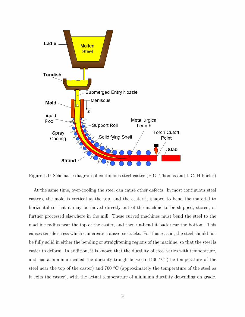
Figure 1.1: Schematic diagram of continuous steel caster (B.G. Thomas and L.C. Hibbeler)

At the same time, over-cooling the steel can cause other defects. In most continuous steel

casters, the mold is vertical at the top, and the caster is shaped to bend the material to

horizontal so that it may be moved directly out of the machine to be shipped, stored, or

further processed elsewhere in the mill. These curved machines must bend the steel to the

machine radius near the top of the caster, and then un-bend it back near the bottom. This

causes tensile stress which can create transverse cracks. For this reason, the steel should not

be fully solid in either the bending or straightening regions of the machine, so that the steel is

easier to deform. In addition, it is known that the ductility of steel varies with temperature,

and has a minimum called the ductility trough between 1400 C (the temperature of the

steel near the top of the caster) and 700 C (approximately the temperature of the steel as

it exits the caster), with the actual temperature of minimum ductility depending on grade.

2

Hence, a common practice for preventing surface cracks is to ensure that the temperature at

the surface in the bender or straightener, where tensile stresses are greatest, is either below

or above this trough.

Another root cause of cracking is the low relative strength of the material at the solid-

ification front. Cracks called “hot tears” can form there, and several criteria have been

developed to predict these hot tears[2]. These criteria can be thought of as conditions on

the temperature history of the steel at the solidification front that determine whether hot

tearing occurs.

Thus, many steel quality and productivity goals can be met by regulating the strand

temperature using the secondary-cooling water sprays. This would appear to be a classi-

cal application for feedback control. Yet, most steel mills only use open-loop methods for

controlling their water sprays. This is because casting presents several key challenges that

modern control theory has not yet developed methods of solving. The most important of

these, I argue, is that the process is inherently distributed and non-linear. As discussed

above, in order to ensure steel process and quality constraints, the temperature of the steel

must be simultaneously regulated at the surface for transverse crack prevention, the interior

for hot tearing prevention, and the center for whale prevention. That is, the entire dis-

tributed temperature profile must be controlled. Moreover, while the classical heat equation

is perhaps the most well-studied partial differential equation (PDE) in the burgeoning field

of distributed parameter control systems, the material in a caster is solidifying. This makes

the system non-linear, and not a small perturbation of the linear heat equation. Therefore,

existing methods for controlling linear parabolic PDEs do not apply.

1.2 Literature review

Previous work on control of solidification in continuous casting can be generally divided

into three categories: numerical optimization methods [3, 4], solutions of the inverse Stefan

problem [5, 6, 7], and feedback control methods [8, 9, 10, 11, 12, 13, 14].

The numerical optimization methods in [3] and [4] can take into account realistic metal-

lurgical constraints and quality conditions. However, since the simulation involved is highly

3

complicated and nonlinear, they cannot realistically run in real-time. The inverse problem,

as solved in [5] and [6] directly and in [7] by minimizing a cost functional, is similarly very

numerically complex and thus limited to design of open-loop control schemes.

The feedback control methods are better suited for real-time control, but the control in

[8] and [9] is simplified to the thermostat-style. The work is mathematically rigorous, but

unfortunately not suited to implementation. Moreover, like the inverse methods [5, 6, 7] and

feedback control method [13], they focus on control of the boundary position, which would

ensure whale prevention, but not necessarily crack prevention. Within the industry, the focus

has been on model-based systems with simple control laws for surface temperature. This

means they have the opposite problem of the previously mentioned approaches, focusing on

surface quality and not whale prevention.

Okuno et al[15] and Spitzer et al[16] each proposed real-time model-based systems to track

the temperature in horizontal slices through the strand to maintain surface temperature at

4–5 set points. Computations were performed every 20 s and online feedback-control sensors

calibrated the system. In practice, these systems have been problematic, owing to the

unreliability of temperature sensors such as optical pyrometers.

Barozzi et al developed a system to dynamically control both spray cooling and casting

speed simultaneously[17]. Feedforward control was used to allow the predicted temperatures

to match the setpoints, but their heat flow model was relatively crude, owing to the slow

computer speed of that time. Optimizing spray cooling to avoid defects using fundamentally-

based computational models was proposed by Lally[18]. At that time, the slow computer

speed and inefficient fundamental computational models and control algorithms made online

control infeasible.

In more recent years, several open-loop model-based control systems have been developed

to control spray-water cooling under transient conditions for conventional thick-slab casters.

These systems employ online computational models to ensure that each portion of the shell

experiences the same cooling conditions. Spray-water flow rates have been controlled in

a thick slab caster using a one-dimensional (1-D) finite difference model[19] that updates

about once every minute. Hardin et al[11] and Louhenkilpi and coworkers[20, 10, 21, 22]

have developed 2-D and 3-D heat flow models for the online control of spray cooling. One

4

model, DYN3D, uses steel properties and solid fraction / temperature relationships based

on multicomponent phase diagram computations[21]. Another, DYNCOOL, has been used

to control spray cooling at Rautaruukki Oy Raahe Steel Works[22].

The controllers involved in these works tended to be fairly simplistic. In [11], the authors

designed a static look-up table to change the water flow rate as a function of surface tem-

perature error. The paper [14] gives little detail on the control methodology. Furenes et al

[13] designed a proportional integral (PI) controller, but in contrast to the other approaches,

only considered the solidification boundary instead of surface temperature.

Although these model-based control systems are significant achievements, none of the

models are robust enough for general use. Each must be tuned extensively on an individ-

ual caster, owing to non-general heat transfer coefficients and the use of ad-hoc heuristic

methods, rather than rigorous control algorithms. None of the previous models uses sensor

data input for the mold water cooling, which is readily available and reliable. Finally, none

of these models has been applied to a thin-slab caster, which has the control problems as-

sociated with higher speed, and where cooling in the mold is more important. The design

of my advisers, co-workers, and I [23, 12] was the first built to work on thin-slab casters,

which tend to have faster speed and consequently require faster model updates. This was

done by adapting a 1-D model instead of trying to make a 2-D model coarse enough to run

in real-time. Surprisingly to us, simple PI controllers with anti-windup sufficed to control

the surface temperature adequately. However, this system cannot directly prevent whales,

as it only considered the surface temperature.

My papers [24] and [25], in contrast, attempt to deal with the distributed 1-D control

problem using Lyapunov stability analysis on the underlying nonlinear Stefan PDE. These

are the first, to my knowledge, results giving control of both the temperature (distributed

throughout the material and not just at the surface) and solidification front at the same time.

The follow-up paper [26] gave some extensions to improve the fidelity of the control-oriented

model with respect to actual continuous casters.

5

1.3 Overview

Several mathematical descriptions of the temperature and solidification in a continuous

caster are discussed below in this chapter. After that, this dissertation is broken up into

three parts, which respectively focus on modeling of the process, control of the process, and

synthesizing the two approaches.

Part I describes the current, state-of-the-art model-based industrial control system. This

system, like the other real-time industry control systems described above, is focused on

dealing with the lack of sensing in continuous casters. Chapter 2 describes the control

system itself, in which a real-time model acts as an open-loop estimator of the surface

temperature of the strand. A simple bank of PI controllers then are used to regulate this

estimated surface temperature. The use of a model as a software sensor in place of a physical

sensor of course requires good accuracy. Chapter 3 discusses the various measurements used

calibrate and validate the model, including trials performed on-site at a thin-slab caster,

and a case taken from the literature. In Chapter 4, the validated model model is used to

perform computational experiments of a thin-slab caster.

In the first part, the control methods are ad-hoc and proven. Part II describes attempts

to use control theory to find provable methods of regulating the temperature. A more

simplistic control-oriented model is considered, which simplifies the PDE for the temperature

error throughout the thickness allowing for easier analysis. Chapter 5 describes a control

law which was proven successful in controlling the entire internal temperature of a slice of

the caster in theory, but un-implementable in practice. The methods behind the design,

though, are put to better use in Chapter 6, in which a much better performing control law

is developed. Then, in Chapter 7, the control-oriented model of Part II is extended to be

closer to the more complicated and accurate model of Part I.

In the final part, I bring the two approaches as close as I am able. The control law of

Part II is applied to a model more closely resembling the model of Part I, and is able to

control the temperature. However, it still requires full-state feedback, which means relying

on the same sort of open-loop estimation described in Part I. Simulations on this control

method, a quantitative analysis of the uncertainty of this open-loop estimator, and some

6

thoughts on possible re-calibration to reduce this uncertainty are given in Chapter 8. In

Chapter 9, I discuss the open issues lying between the completed work and implementation,

giving some unproven conjectures and describing a complete output feedback solution for

the slice problem, which works in simulation but is as yet unproven. Other suggestions for

future work and conclusions, are also offered.

1.4 Process model

The solidifying steel in a continuous slab caster, called the strand, is rectangular in shape.

While dimensions may vary between casters and applications, the strand will typically have

a thickness and a width on the order of 0.1 m and 1 m, respectively. The solidification length

will vary with steel composition and casting speed, but is typically on the order of 10 m. The

temperature evolution for the strand in this domain is three dimensional, and must take into

account, at the least, heat diffusion, advection at the casting speed, and the phase change.

However, due to the large aspect ratio of slabs, the problem reduces to two dimensions in

most of the strand. A scaling argument can be used to show that advection in the casting

direction dominates over heat diffusion in that direction, further reducing the problem to a

one-dimensional “slice” that moves through the strand at the casting speed. Finally, I will,

at least for most of this dissertation, assume that the slice temperature is symmetric, and

only consider the region between the strand surface and center. A more detailed discussion

of this modeling setting can be found in [27].

1.4.1 Enthalpy PDE

In this dissertation, the 1-D temperature within the slice will be denoted as T (x, t), with

0 ≤ x ≤ ` and t ≥ ∞, where x = 0 and x = ` correspond to the outer surface and the center

of the strand, respectively. As discussed above, the control objective for this process is to

match a temperature profile that meets multiple criteria governing final product quality.

Determining a suitable reference profile is a difficult task on its own, and beyond the scope

of this dissertation. For now, assume that a metallurgist has provided, typically through

7

prior experience with the caster and steel grade, a temperature profile that produces good

quality steel under nominal conditions. The goal of the controller, then, is to match this

reference temperature profile in response to changes in initial conditions due to variations

upstream of the spray chamber in the ladle, tundish, and mold.

When solidification is not present, the temperature of the material evolves according to

the classical (linear parabolic) heat equation, in which heat diffuses through the material

based on Fourier’s law. In this linear heat equation, the material absorbs thermal energy

proportional to its (assumed to be) constant specific heat. When solidifying, in contrast,

the material stores an additional amount of energy called the latent heat, which must be

accounted for.

The thermodynamic energy of the material is called enthalpy. In a single-phase material,

the enthalpy is approximately proportional to the temperature, with the constant of pro-

portionality equal to ρcp where ρ is the density of the material and cp is the specific heat.

However, for a solidifying pure material, there is a step change in enthalpy at the melting

temperature, Tf , equal to the latent heat of solidification, hf . Altogether, this means the

enthalpy, denoted h, can be described as a function of temperature:

h(T ) :=

cpT T < Tf

cpT + hf T > Tf

(1.1)

Then the following PDE models the evolution of temperature within the slice:

(ρh(T (x, t)))t = kTxx(x, t) , x ∈ (0, `) , (1.2)

Tx(0, t) = u(t) , Tx(`, t) = 0, (1.3)

T (x, 0) = T0(x) (1.4)

where k is the thermal conductivity. The controlled input to the process u is Neumann

boundary condition on the left-hand side. In the continuous caster, this is directly propor-

tional to the heat flux removed from the steel at the surface.

This PDE is difficult to analyze mathematically due to the discontinuity in the function

8

h(T ) . In [28], the authors prove that the state operator forms a semi-group on L1. This

does not necessarily imply that a strong solution to the PDE exists. An advantage of this

formulation, though, is that it is easier to simulate numerically. The simulations in Part II

were all performed on this method, as described in Appendix A.

A second advantage of the enthalpy formulation is that it generalizes well to alloys. Alloys

do not have a single melting temperature. Instead, they are partially solid and partially liquid

in the so-called “mushy” temperature range. This can be accounted for by adjusting (1.1)

to have a gradual increase from latent heat rather than a step change.

An alternative to (1.1)–(1.4) that is conceptually the same is to use an effective specific

heat. Mollifying (1.1) slightly gives a similar function h∗(T ) that is differentiable. Define

the effective specific heat, c∗p to be this derivative,

c∗p(T ) :=dh∗

dT(1.5)

Then, using the chain rule, the equivalent of (1.2) using this notation is:

ρc∗p(T )Tt(x, t) = kTxx(x, t) , x ∈ (0, `) . (1.6)

The effective specific heat c∗p(T ) is nonlinear, being much larger during phase changes than

at other temperatures. This equation is therefore quasilinear and parabolic[29] in nature.

This PDE is the one numerically calculated in Part I.

1.4.2 Stefan problem

A simpler PDE describing this system is known as the Stefan problem, which treats the liquid

and solid as occupying separate subdomains. The boundary between the two moves over

time as the material solidifies. The Stefan problem uses an additional differential equation

for this solidification front to enforce the energy balance including latent heat[30], which

requires the temperature gradient to be discontinuous at the moving boundary.

For the Stefan problem, denote the position of the boundary between solid and liquid

phases as s(t). Then the following PDE models the evolution of temperature within the

9

slice:

Tt(x, t) = aTxx(x, t) , x ∈ (0, s(t)) ∪ (s(t) , `) , (1.7)

T (s(t) , t) = Tf , Tx(0, t) = u(t) , Tx(`, t) = 0, (1.8)

T (x, 0) = T0(x) (1.9)

s(t) = b(Tx(s−(t) , t

)− Tx

(s+(t) , t

)), s(0) = s0 (1.10)

In physical terms, Tf is the melting temperature, a is the thermal diffusivity, and b = k/ρhf .

Both of these physical quantities are strictly positive.

Existence and uniqueness of solutions to the Stefan problem, in contrast to the enthalpy

method, is very well studied[30, 31, 32]. Moreover, for the purposes of designing of a model-

reference controller, the resulting error system from the enthalpy PDE is fully nonlinear in

a way that is difficult to analyze. By comparison, the reference error system for the Stefan

problem, described in Part II, has a similar form to the Stefan problem itself, linear on

sub-domains with nonlinear moving boundaries. For this reason, it is used for the control

design in Part II.

Since the moving boundary point s(t) in the Stefan problem would require a time-varying

spatial discretization scheme, the enthalpy PDE (1.2), which can be used on a fixed grid, is

used for simulations. This means that control design and simulations are for different PDEs,

but the two are practically equivalent. Appendix A verifies this by comparing an analytical

solution to the Stefan problem with an equivalent simulation of the enthalpy PDE.

10

Part I

State-of-the-art industrial model and

control for steel continuous casters

11

CHAPTER 2

STATE-OF-THE-ART INDUSTRIAL CONTROLMETHOD: CONONLINE

Current work within the steel industry on control of water sprays in continuous steel casting

has focused on the lack of reliable sensing. As of now, no reliable measurement-feedback

system has been implemented in an operating steel caster due to the difficulty of installing

and maintaining reliable temperature sensors. As a result, researchers and engineers focused

on creating a “software sensor,” an accurate model fast enough to run in real time, as a

replacement for physical sensors. This chapter is based on the papers [23], [12], and [33],

which originally presented a breakthrough real-time model and control system for the Nucor

Steel Decatur continuous steel casters.

2.1 Introduction

This chapter presents a control system called Cononline that has been developed to con-

trol spray cooling in thin-slab casters, and has recently been implemented at the Nucor

Steel casters in Decatur, Alabama. This system features an efficient fundamentally-based

solidification heat-transfer model of a longitudinal cross section of the strand as a software

sensor of surface temperature. The model, called Consensor, estimates the entire shell sur-

face temperature and solidification profile in real time, based on tracking multiple horizontal

slices through the strand with a subroutine version of a previous computational model,

CON1D[27]. Then, 10 independently-tuned proportional-integral (PI) controllers together

with classical anti-windup are designed to maintain the shell surface temperature profile at

the desired setpoints in each of the 10 spray cooling zones throughout changes in casting

speed, steel grade, and other casting conditions.

In addition to the software sensor and the controller, this real-time spray-cooling control

12

system also includes a monitor interface that provides real-time visualization of the predicted

shell surface temperature predictions, the predicted metallurgical length, spray-water flow

rates, setpoints, and other important information to the operator. The monitor also allows

operator input through the choice of temperature setpoints. The system uses shared memory

and Transmission Control Protocol / Internet Protocol (TCP/IP) server and client routines

for communication among the software sensor, controller, monitor interface and the caster

automation systems.

2.2 Control system overview

The dynamic control system for thin-slab casters is based on the control diagram shown

in Figure 2.1. The core of the system is a software sensor based on the CON1D heat-

conduction model. The software sensor, Consensor, provides a real-time estimate/prediction

of the strand state, including the shell surface temperature profile and metallurgical length.

It updates based on all the available casting conditions, which include: 1) conditions updated

every second, including mold heat flux, casting speed, tundish temperature (for superheat),

slab width, and spray flow rates; 2) the steel composition, which is updated during ladle

exchanges; and 3) conditions updated only when the software sensor is calibrated, including

slab thickness, the mold, roll, and spray nozzle configuration and parameters in the heat-

transfer coefficient models. The estimated shell temperature profile is then compared against

a pre-determined surface-temperature profile setpoint. The mismatch between the estimate

and the setpoint, i.e. the tracking error, is then sent to a dynamic controller to compute

the water flow rate command required to drive the mismatch to zero. Finally, the computed

command set of spray-water flow rates is sent to the spray zone actuators in the operating

caster, to the Monitor program for visual display to caster operators, and also to the software

sensor for estimation at the next second.

13

Human-Machine Interface

Shell thickness and surface temperature estimation

Spray water flow rates

Setpointoptions

Software Sensor2-D transient thermal model

(200 moving 1-D slices)

steelsteel P steel

T TC k

t x xρ ∗ ∂ ∂ ∂ = ∂ ∂ ∂

ControllerSeparate PI controller for each spray zone

caster data

ΣΣΣΣ+

-

Caster

AUTOMATIC CONTROL LOOP

MAN/MACHINE SUPERVISORY

LOOP

SetpointGenerator

Surface temperature setpoint

Pjk

Ijk ( )

0

tdt⋅∫

ΣΣΣΣ

ΣΣΣΣ

Saturation

ΣΣΣΣ +-awjk

Figure 2.1: Overview of Cononline control system with software sensor, Consensor, and PIcontroller, Concontroller.

14

Table 2.1: Separate software programs in Cononline control system

Program name FunctionConsensor estimating/predicting the profile of strand temperature and shell

thickness based on CON1DConcontroller computing the required spray water flow rate to maintain tem-

perature setpointCononlineMonitor displaying in real-time Consensor predictions, computed water

flow rate and casting conditionsCommServer working with CommClient programs to transfer data between

computersCommClient working with CommServer programs to transfer data between

computersActiveXServer TCP server working with monitor programs to transfer data be-

tween controller server and PCs running CononlineMonitor

2.3 System Architecture and Implementation

The control diagram in Figure 2.1 is realized in Cononline, which consists of several pro-

grams running in real time on several different linked computers. As shown in Figure 2.2,

the main system hardware consists of two servers. The “Model” server runs the software

sensor, Consensor, on the CentOS operating system. The Consensor model is a FOR-

TRAN program, owing to its computational efficiency. The “Controller” server runs the

controller, Concontroller, on the Slackware Linux operating system. Concontroller is writ-

ten in C to take advantage of real-time OS commands not available in FORTRAN. The

various programs communicate through “shared memory,” which is a block of memory with

the same contents on each computer that is accessible by any program and is updated con-

tinuously via TCP/IP by programs CommServer and CommClient. A separate TCP server

program called ActiveXServer transmits the information to up to 16 Windows PCs running

a human-interface Visual C# program called CononlineMonitor. CononlineMonitor, which

can be run independently on multiple computers, displays the results and accepts user input.

These programs are listed in Table 2.1.

As shown in Figure 2.2 in the “Caster Automation Systems” block, the control system

can be tested and tuned using real caster data while the existing controller manages the

secondary cooling. During this so-called “shadow mode” of operation, many causes of crashes

15

Controller Computer

(Slackware Linux)

CommServer

shared memory

CommServer

CONCONTROLLER

ActiveXServer Model Computer

(CentOS Linux)

shared memory

CommClientCONSENSOR

Windows Computers

CononlineMonitor

CononlineMonitor

TCP/IP connection

Shared memory connection

Legend:

Caster Automation Systems

CommClient

Current control logic

Figure 2.2: Cononline system architecture.

16

and errors were identified and solved, with the help of checks to ensure that input data stays

within reasonable bounds. The system is now very robust and maintains stable operation

through all sets of conditions tested, including serious disruptions or errors in input data.

In either shadow or direct control mode, the caster automation systems send casting con-

ditions, discussed in Section 2.4, once every second to the Controller server via CommClient.

The casting conditions are received by CommServer in the Controller server and relayed to

the Model server via its CommClient. These data are available immediately to the sensor

and controller via the shared memory in each server. The software sensor then estimates the

shell temperature distribution in approximately 0.5 s. The controller reads this distribution

from shared memory and computes the spray-water flow rates to maintain the selected set-

points, every 1 s. To ensure timely updating, data are exchanged between the two servers

approximately 10 times per second with transmissions taking less than 20 ms each.

The predicted shell surface temperature and shell thickness profiles are transmitted via

ActiveXServer to any CononlineMonitor programs running, to be displayed on the operator

console and elsewhere in real time. The CononlineMonitor programs update every 3 s, which

is slower than the 0.1 s updates between the primary Cononline servers in order to lessen

transmission traffic on the steel mill’s general network. The spray-water flow-rate commands

are also sent to the caster automation systems to be applied by the flow actuators in the

actual caster. Finally, changes to the temperature setpoints or control mode requested

by the operator through a CononlineMonitor program are sent to the other computers, in

preparation for the next time increment.

2.4 System Components

2.4.1 Heat transfer model — CON1D

CON1D is a simple but comprehensive fundamentally-based model of heat transfer and

solidification of the continuous casting of steel slabs, including phenomena in both the mold

and the spray regions[27]. The accuracy of this model in predicting heat transfer with

solidification has been demonstrated previously through comparison with analytical solutions

17

of plate solidification and plant measurements[27, 34]. Because of its accuracy, CON1D has

been used by the steel industry to predict the effects of changes in casting conditions on

solidification and to develop practices to prevent problems such as whale formation[35].

The simulation domain in this work is a transverse slice through the strand thickness that

spans from the shell surface at the inner radius to the outer radius surface. The CON1D

model computes the complete temperature distribution within the solid, mushy, and liquid

portions of the slice as it traverses the path from the meniscus down through the spray

zones to the end of the caster at torch cutoff. CON1D uses an explicit-in-time, centered-

in-space finite-difference algorithm to solve the 1-D transient heat conduction equation with

solidification included via effective specific heat, i.e. (1.6).

CON1D is actually much more complicated than the simplified PDE (1.6). A brief

overview is given below, but for more detail the reader is directed to [27]. The effect of

non-uniform distribution of superheat is incorporated using the results from previous 3-

D turbulent fluid flow calculations within the liquid pool. Thermal properties vary with

temperature according to composition and phase-dependent material property models. Mi-

crosegregation effects are included via a modified Clyne-Kurz model [36]. Thus, rather than

(1.5), the effective specific heat is

c∗p(T ) := cp(T )− hfdfs

dT

where the temperature dependent specific heat cp(T ) and solid fraction fs(T ) come from ma-

terial property and microsegregation models, respectively. These solidification and thermal

property models depend on the steel composition.

Using a more general temperature-dependent solid fraction means the material may have

solidus temperature (solid fraction 1, or completely solid) different from its liquidus temper-

ature (solid fraction 0, or completely liquid), rather than changing immediately at a single

melting temperature. That is, there is not a clearly-defined boundary between liquid and

solid. In the simulations in this part of the dissertation, shell thickness is defined by a solid

fraction of 0.7, which is commonly considered to be solid enough to prevent whales. This is

justified also by comparison with measurements of the caster in the next chapter.

18

The numerical method is kept efficient by using a post-time-step correction to better

enforce the energy balance at the liquidus temperature, where the solid fraction slope is

steepest. Good accuracy is achieved using a grid spacing, ∆x, of approximately 1 mm and

finite-difference time-stepping size, ∆t, of 0.03 s. With this tool used as a subroutine by the

software sensor, Consensor, the closed-loop diagram of Figure 2.2 takes the form shown in

Figure 2.3. The model box contains the explicit discretized form of Equation (1.6) solved

by CON1D. The initial condition (IC) is the pour temperature Tpour, measured in the

tundish, and boundary conditions (BC) are summarized below, with further detail provided

elsewhere.

I will denote the CON1D numerical prediction of the temperature as Ti (x, t). In order

to produce an estimate for the entire caster, the software sensor uses multiple simultaneous

runs of CON1D, hence the subscript i indicates the temperature history of a particular

slice.

Material properties

The temperature and phase-dependent thermal properties are described in [27] and plotted

for a representative low (0.05 wt-%) Carbon steel in Figure 2.4. Phase fractions during

solidification were found using a simple microsegregation model[36]. Density is constant in

the temperature calculation. The Thermal Linear Expansion (TLE) function, needed as a

post processing step to predict the average shrinkage, is based on measurements from the

literature. For a material of length L, the TLE is the relative change in length when the

temperature is changed from a reference temperature,

TLE(T ) :=∆L(T )

L(Tref):=

L(T )− L(Tref)

L(Tref)(2.1)

To get this from the measurements of density, at a given temperature, the density ρ(T )

is calculated as the weighted average of the density of the individual phases using published

19

Fig

ure

2.3:

Clo

sed

loop

blo

ckdia

gram

wit

hC

onse

nso

rpre

dic

tor

and

Con

contr

olle

rP

Ico

ntr

olle

rban

k.

20

empirical models[37, 38, 39], and from this the TLE is

TLE(T ) = 3

√ρ(Tref)

ρ(T )− 1 (2.2)

In Figure 2.4, this reference is chosen to be the liquidus temperature, but other reference

densities could have been chosen, and in fact will be in Section 3.2.

Boundary conditions in the mold

In previous work, the CON1D model computes the surface heat flux within the mold region

by solving a two-dimensional heat equation in the mold and several mass and heat balance

equations within the interfacial gap[27, 40]. Its accuracy to predict mold heat transfer

has been verified against a full three-dimensional finite element analysis, as well as plant

measurements[34]. It is not currently possible to solve all of these equations in real-time, so

a simpler model was developed to accurately yet quickly define the surface heat flux profile

in the mold.

In a continuous caster, the average heat flux in the mold can be easily calculated from the

measured temperature rise and flow rate of the cooling water, and is supplied to Consensor

through the caster automation systems in real time. The heat flux profile as a function of

time, qmold(t) (MW/m2), is fit with the following empirical function of time to match the

average measured mold heat flux, qmold (MW/m2). This function is split into a linear portion

and an exponential portion:

−k∂Ti(±`, t)∂x

= qmold :=

q0 − qa · (t− t0i ) , 0 ≤ t− t0i < tc

qb · (t− t0i )−n

, tc < t− t0i < tm(2.3)

where t0i is the start time for the slice and hence t− t0i is the time since the slice was at the

meniscus. There are three fitting parameters. The first is n, which controls the shape of the

curve and is currently chosen to be 0.4. The initial heat flux, q0, is the maximum heat flux

at the meniscus, calculated as:

q0 := qfac · qmold (2.4)

21

00.250.5

0.751

Pha

se fr

actio

n

600

700

800

900

Spe

cific

hea

t(J

/kg−

K)

1300 1350 1400 1450 1500 155030

35

40

Temperature (oC)

The

rmal

con

duct

ivity

(W/m

−K

)

liquidferriteaustenite

−0.02

−0.01

0

TLE

(m/m

)

Figure 2.4: Thermodynamic properties of 0.05 wt-% Carbon steel, using the referencedmicrosegregation and material property models.

22

where qfac is another parameter, currently set to 2.3. The total time spent in the mold tm is

calculated by

tm :=zm

vc

(2.5)

where zm is the mold length and vc is the casting speed. For complete accuracy, this should

be defined by an integral equation, but that would require knowing future casting speeds

while the slice is in the mold. This method allows real-time prediction of temperatures in

the mold, but will cause additional error during sudden changes in casting speeds. Using

this approximation for tm, the duration of the linear portion, tc, is assumed to be

tc := tfac · tm (2.6)

where tfac is the third parameter, currently set to 0.07.

With the fitting parameters chosen, the intermediate parameters qa and qb are defined

below, calculated to keep the curve continuous and match the total mold heat flux in the

mold with the area beneath the curve.

qa :=q0 · (tc)n · (tm)1−n − (1− n) · qmold · tm − n · q0 · tc

(tc)1+n · (tm)1−n − 1

2(1 + n) · (tc)2 (2.7)

qb := q0 · (tc)n − qa · (tc)1+n (2.8)

Figure 2.5 compares heat flux profiles predicted with this new model to previous measure-

ments in thin-slab casting molds[34, 41].

Boundary conditions in the spray zone

Below the mold, heat flux from the strand surface is given by

−k∂Ti(±`, t)∂x

= htotal · (Ti(±`, t)− Tamb) (2.9)

where Tamb is the ambient temperature and htotal (W/m2K) varies greatly between each pair

of support rolls and consisting of four components: spray nozzle cooling (based on water

23

0

1

2

3

4

5

6

7

8

9

0 100 200 300 400 500 600 700 800 900

Distance Below Mensicus (mm)

Hea

t F

lux

(MW

/m2)

Park heat flux [2.82 MW/m2]

Park heat flux (CONONLINE)

Santillana heat flux [2.63 MW/m2]

Santillana heat flux (CONONLINE)

Figure 2.5: Comparison of Cononline predicted mold heat flux, Equations (2.3)–(2.8), withmeasurements from [34] and [41].

24

Surface Temperature (°°°°C)

Dis

tan

ce (

mm

)

1000 1100 1200 1400

1

300

1

200

1

100

Slab

Roll

Spray nozzle

natural/forced convection, hconv

radiation, hrad

spray impinging, hspray

roll contact, hroll

Heat Transfer Coefficient

Figure 2.6: Illustration of heat transfer coefficients in spray zone.

flux) hspray, radiation hrad, natural convection hnconv, and heat conduction to the rolls hroll,

as shown in Figure 2.6. Incorporating these phenomena enables the model to simulate heat

transfer throughout the entire continuous casting process.

Spray cooling heat extraction is specified as the following function of water flow rate[42]:

hspray := A · (Qspray)c · (1− bTspray) (2.10)

where Qspray (L/m2s) is spray water flux and Tspray is the temperature of the spray cooling

water (C). For air-mist nozzles, this work assumes that air flows are consistent functions of

water flow, so are not considered separately. Finding parameters to accurately predict spray

cooling heat extraction presents a significant challenge that has been the focus of several

previous experimental studies. In Nozakis empirical correlation[42], A = 0.3925, c = 0.55,

and b = 0.0075, which has been used successfully by other modelers[43, 42, 44]. The well-

25

known drop in heat extraction from the sprays on the bottom surface of the strand, and the

increase in heat extraction due to the Leidenfrost effect at lower temperatures, both can be

accommodated, but await additional measurements.

Radiation, hrad, is calculated by:

hrad := σ · ε · (Ti,sK + TambK) ·(T 2i,sK + T 2

ambK

)(2.11)

where Ti,sK is the surface temperature of the strand, Ti(±`, t), expressed in Kelvin, σ is the

Stefan-Boltzman constant (5.67 x 10-8 W/m2K4), ε is the emissivity of the strand surface,

assumed to be 0.8, and TambK is ambient temperature, 298 K. Natural convection, hrad, is

typically much smaller than the other heat losses, so is treated here as a constant 8.7 W/m2K.

The heat transfer coefficient extracting heat into each roll, hroll, is expressed as a fraction,

froll, of the total heat extracted. This fraction is calibrated separately for each spray zone[27]:

hroll :=(hrad + hnconv + hspray) · Lroll + (hrad + hnconv) · (Lzone − Lspray − Lroll)

Lroll · (1− froll)(2.12)

where Lzone, Lspray, and Lroll, are the total lengths in the casting direction of the entire spray

zone, the nozzle sprays, and roll contact, respectively. All of these, and also froll may be

different in each segment of the caster.

Increasing froll increases the severity of local temperature drops beneath the rolls. Severity

also depends on the length of the roll contact region, Lroll, based here on assuming a contact

angle with the roll, θroll of 10. Beyond the spray zones, heat transfer simplifies to only

include radiation and natural convection. Calibration of these results is discussed in the

next chapter.

2.4.2 Software sensor — Consensor

The function of the software sensor is to accurately predict the temperature distribution in

the strand in real time. The program Consensor was developed to produce the temperature

profile along the entire caster (z) and through its thickness (x) in real time (t), by exploiting

CON1D as a subroutine. It does this by managing the simulation of N different CON1D

26

Figure 2.7: Illustration of Consensor simulation domain.

slices, each starting at the meniscus at a different time to achieve a fixed z-distance spacing

between the slices. This is illustrated in Figure 2.7 using N = 10 slices for simplicity.

The goal for Consensor is to provide an updated temperature estimate, T (x, z, t), every

∆t seconds. The surface temperature estimate T is assembled from individual CON1D slice

profile histories Ti, as follows.

During each time interval, the N different CON1D simulations track the evolution of

temperature in each slice over this interval, given the previously-calculated and stored tem-

perature of that slice at the start of the interval. The computation time required is about

the same as just one complete CON1D simulation of the entire caster length, which takes

about 0.6 seconds on the CentOS “Model” server when casting at 4.5 m/min. During pro-

gram startup, the simulation for slice i + 1 begins when slice i passes 75 mm from the

27

meniscus. After startup, a new slice begins immediately from the meniscus whenever a slice

reaches the end of the caster. Currently, Consensor always manages exactly 200 slices, which

corresponds to a uniform spatial interval of 75 mm along the overall simulation domain for

the Nucor Decatur casters, ztotal = 15 m, covering the space between the top of the mold

and the shear cut. The complete temperature history for each slice is stored from when it

started at the meniscus, t0i , to the current time, t. To assemble the complete temperature

profile needed each time interval requires careful interpolation of the results of each slice at

different times.

When plotted on a two-dimensional t-z grid, the desired output domain of the software

sensor is a horizontal line, as shown in Figure 2.8. For instance, at time t∗ the sensor must

give a prediction T (x, z, t∗) for the entire caster length, 0 ≤ z ≤ zc. However, the surface

temperature included in a single slice history from CON1D traverses a monotonic-increasing

curve in the t-z plane. At constant casting speed vc, these curves are straight diagonal lines

with slope 1/vc. Figure 2.8. shows two such lines representing two slices created at times t01

and t02. It is clear from Figure 2.8 that each run of CON1D contributes only one temperature

profile to the desired software sensor output at each time, T (x, zi(t) , t∗), where zi(t) is the

location of the ith slice at time t, which is calculated by

zi(t) :=

∫ t

t0i

vc(τ) dτ, i = 1, . . . , N (2.13)

With constant casting speed, this integral simplifies to vc · (t− t0i ). Data points in the tem-

perature profile estimate such as (x, zi(t∗) , t∗), which come directly from CON1D output,

can be thought of as “exact” estimation points.

Figure 2.9 illustrates the error introduced by interpolating spatially between these exact

points. The 75 mm span between slices in this work can pass over the temperature dips

and peaks caused by the roll and spray spacing, resulting in errors of 100 C or more. This

problem is overcome by delay interpolation, interpolating temporally between the latest

temperature histories available from each CON1D slice, described as follows and illustrated

in Figure 2.8 using N = 2 slices.

For locations between the exact estimate points, the surface temperature is approximated

28

Figure 2.8: Illustration of Consensor delay interpolation technique.

29

Figure 2.9: Linear interpolation of slice surface temperatures, with 200 slices in 15 m longNucor Decatur caster.

30

at the current time using the most recent available temperature at that location from the

CON1D slice histories. Applying this method everywhere along the caster, the control-

oriented steel temperature profile prediction T (x, z, t) is obtained at any time t:

T (x, z, t) = Ti(x, z, ti(z)) (2.14)

where ti(z) is the time when the ith slice was located at the distance z from the meniscus,

which is the inverse of Equation (2.13)

ti(z) := t0i +

∫ z

0

1

vc

dζ (2.15)

For constant casting speed, this simplifies to t0i + z/vc.

Figure 2.8 illustrates this process at time t∗, with constant casting speed for simplicity.

In the figure, there are two slices that began at different times, giving temporally-exact

estimates at two locations at time t∗. The point (z∗, t∗) lies between the locations of these

exact estimates, so according to the delay interpolation scheme, the surface temperature at

this point is approximated by the surface temperature of slice 1 when it passed the distance

z∗ from the meniscus. Thus, the temperature T1(x, z∗, t0i + z∗/vc) from the history of slice 1

is used as the the temperature profile estimate t(x, z∗, t∗).

The delay interpolation error introduced at location z∗ in Figure 2.8 is the temperature

change at this location from time t1(z∗) to t∗, which is a function of the extent of transient

effects in the laboratory frame, and slice spacing. An example of this error is shown in

Figure 2.10 under the worst-case scenario, shortly after a sudden drastic decrease in casting

speed. In the figure, slices 151, 152, and 153 were consecutively created slices. Slice 153 is the

newest, and has only traveled 2.10 m from the meniscus at the time the data was collected.

Slice 152 is the second newest, and has traveled slightly further, 2.22 m from the meniscus.

Slice 151 is the oldest. Therefore, before 2.10 m, Consensor takes the temperature and shell

thickness from the history of slice 151. Between 2.10 m and 2.22 m, the history of slice 152 is

taken. Above 2.22 m, the history of slice 151 is used. Because the strand is cooling quickly

after the speed dropped suddenly, slice 153 is much colder than slice 152, which is much

31

600

800

1000

1200

Sur

face

tem

epra

ture

(o C)

2.00 2.05 2.10 2.15 2.20 2.25 2.3015

20

25

30

Distance from meniscus (m)

She

ll th

ickn

ess

(mm

)

slice 151 slice 152 slice 153 interpolated

Figure 2.10: Illustration of transient estimation error due to Consensor delay interpolationtechnique.

colder than slice 151. This leads to the jumps in temperature and shell thickness at the

points where Consensor switches from an older slice to a newer one. The most reliable data

is the newest, i.e. at the current location of each slice, just before the jumps.

It follows that slices should be evenly distributed to minimize the approximation error,

and that the magnitude of this error decays to zero during steady operation. Even during

times of extreme transients, this error is easily recognized by operators from the jagged

appearance of the temperature profile, as seen in Figure 2.10. During operation, the distance

simulated during each time interval increases with casting speed, but is usually less than the

distance between slices. Specifically, the 75 mm span in this work is achieved only for speeds

of 4.5 m/min or more. At lower speeds, the points further along each jag in the casting

direction are most accurate, because they contain the most recent temperature estimates.

32

2.4.3 Control algorithm — Concontroller

Because heat transfer between slices is negligible, a simple set of uncoupled single-input-

single-output (SISO) controllers can be used to control the spray-water flow rates to minimize

the error between the Consensor prediction and a setpoint temperature profile. A single

multi-input-multi-output (MIMO) controller is another option, but is more complicated to

design and implement and does not offer much better performance.

The temperature control problem can be regarded as a disturbance rejection problem,

in which the heat flux from the liquid core inside the strand can be treated as a slowly-

changing disturbance and the control goal is to maintain shell surface temperature under

this disturbance. In light of this observation, the control law is simply chosen as the stan-

dard Proportional-Integral (PI) control. Here, the integral part is necessary for maintaining

the surface temperature with no steady-state error under a constant setpoint and rejecting

constant disturbances. Derivative control, which is normally introduced to increase damping

and stability margin, is not used since the system itself is well damped, owing to the high

thermal inertia of the solidifying steel strand.

An important feature of the caster spray configuration is that the rows of individual spray

nozzles are grouped into Nzone spray zones according to nozzle location and control authority

(which depends on how nozzles are connected via headers and pipes to a given valve). Each

individual spray zone corresponds to an area where the spray water to the nozzles has a single

inlet valve. This means that all rows of nozzles in a zone have roughly the same spray-water

flow rate and spray density profile. This configuration is shown in Figure 2.11 and listed in

Table 2.2, where uj refers to the jth spray zone[45]. High in the caster, where the strand is

vertical, nozzles on the inner and outer radii are part of the same spray zone. For the Nucor

Decatur casters, this is the case for the first 4 spray regions. The lower 3 zones each have

a separate zone and spray command for the inner and outer radius surfaces. Therefore, a

total of Nzone = 4 + 2 × 3 = 10 independent PI controllers are needed. The parameters of

each controller are tuned separately to meet the control performance in each zone, and are

listed in Table 2.3. These gains were chosen by assigning initial values based on the average

total water flow through each zone, and then tuning by trial and error in offline simulations

33

Figure 2.11: Diagram of spray zones in the Nucor Decatur casters.

and later plant trials. Cononline provides model-based control only for the center-line zones.

Based on these 10 control signals, the spray flow rates for other zones across the strand

width are prescribed as a function of slab width using separate logic. Generally, the flow

rates per unit area are kept constant across the width, except in zones containing strand

edges, where they are turned down slightly to lessen overcooling of the slab corners.

In accordance with this spray area configuration, the control algorithm proceeds through

the following steps (see also Figure 2.3). At each time, t, the inner and outer radii shell

surface temperature profile estimate, T (xzone, z, t), is obtained by the software sensor as the

multi-slice temperature calculation aggregated with the interpolation procedure illustrated

in Figure 2.8. The desired shell surface-temperature profile setpoints will be denoted as

T s(z, t), and are discussed in more detail in Section 2.5.

34

Table 2.2: Controller assignments [45].

Spray Zone Segment Side Lspray Lzone Wspray Controller(m) (m) (m)

1 foot rolls both 0.05× 2 0.090× 2 1.640 u1

2 upper bender both 0.25× 2 0.827× 2 0.987 u2

3 lower bender both 0.30× 2 1.061× 2 1.008 u3

4 segment 1 both 0.25× 2 0.946× 2 1.620 u4

5 segments 2/3inner 0.50 2.130 1.620 u5

outer 0.50 2.130 1.680 u6

6 segments 4/5inner 0.50 2.356 1.680 u7

outer 0.50 2.356 1.680 u8

7 segments 6/7inner 0.50 2.986 1.680 u9

outer 0.50 2.986 1.680 u10

1. Calculate the average tracking error for each zone:

∆Tj(t) :=

∫zone j

(T s(z, t)− T (xzone, z, t)

)dz

Lzone

(2.16)

where Lzone and xzone change for each zone, j, as in Table 2.2. For outer radius zones

xzone = −`, and for inner radius zones xzone = `. In the upper caster, where the spray

zones cover both sides of the strand, the integral must be done over both sides.

2. Calculate the spray-water flow rate command for the next time interval, via the classic

PI control law:

uj(t+ ∆t) := uPj (t+ ∆t) + uI

j(t+ ∆t) (2.17)

where the proportional and integral components are defined as:

uPj (t+ ∆t) := KP

j ·∆Tj(t+ ∆t) (2.18)

uIj(t+ ∆t) := uI

j(t) +KIj ·∆Tj(t+ ∆t) ·∆t (2.19)

where (2.19) is a discrete-time integral over the time interval ∆t (1 s, currently). The

proportional and integral gains for each controller, KPj and KI

j , respectively, are given

in Table 2.3.

35

Table 2.3: Controller gains

Controller KPj KI

j

1 0.4 0.42 2.0 1.03 1.2 0.64 0.5 0.4

5–6 5.0 0.1257–8 5.0 0.59–10 1.8 0.8

Note that (2.19) is a recursive definition, and so the initial settling time of the PI controller

will depend on the initial choice of the control output, uIj(0), supplied when the control

algorithm begins its calculations. During casting startup, PI control starts in a given zone

only after steel has entirely filled the zone. Before this time, control is chosen based on the

existing spray-table control method. When the PI control calculation begins for zone j, the

spray-water flow rate from the spray table is assumed as an initial value of uIj, to reduce the

initial settling time.

The control command uj, which is the requested water flow rate to spray zone j in L/s,

is sent to the caster automation systems. The flow rate through the valve governing spray

zone j, u′j(t), is measured by the caster automation systems and sent to Consensor in order

to estimate the surface heat flux using Equation (2.10). The spray-water flux is currently

assumed uniform over the nozzle footprints in each zone, and is calculated by:

Qspray =uj

LsprayWspray

(2.20)

where Qspray is the spray-water flux in each row of nozzles in spray zone j. The width,

Wspray, and length, Lspray, of the area of the steel surface upon which sprays impinge may

be different for each zone j, and are given in Table 2.2 for the Nucor Decatur casters.

2.4.4 Visualization — CononlineMonitor

The monitor is an important component in the control system because it provides real-time

display of many variables, setpoints, and results, permitting plant operators and metallur-

36

gists to monitor the caster and the control system performance and to make adjustments

as needed. In addition to the instantaneous casting conditions, the monitor displays for

both the outer and inner radii: the estimated shell surface temperature profiles, the cor-

responding temperature setpoints in each zone, estimated shell thickness growth profile,

controller-requested water flow rates control commands in each zone, the corresponding

measured flow rates, and other parameters. To avoid network traffic problems, the refresh

rate on the Monitor is 3 seconds.

Figure 2.12 shows typical screen shots of both monitor interface windows. Figure 2.12a

shows the “profile screen.” This screen serves two purposes. The first purpose is to relay

key simulation outputs to the operators and plant engineers. Important caster parameters

such as casting speed and final solidification point are noted at the top of the screen. The

two opposing shell profiles form the estimated V-shape of the real liquid pool. Together with

the superimposed temperature profiles, it is easy to visualize the state of the caster.

The second purpose of the profile screen is to supply an interface for operator input to

the controller, via a drop-down box of setpoint generation options, and individual controls

to change the temperature setpoint in any zone manually. The controller can generate

temperature setpoints in several ways, as described in the next section. Figure 2.12b shows

the “parameter screen,” which displays the most important caster measurements input to

the model. This allows for easy checking of the casting conditions, and TCP/IP server and

client operation.

The importance of the monitor as part of the control system should not be underestimated.

By presenting accurate information to the operator in real time in a natural visual manner,

this system empowers the operator to react better to unforeseen situations. Ultimately, a

truly “expert” caster control system should recognize and take appropriate action to prevent

potential problems, in addition to controlling sprays to maintain surface temperature.

2.5 Additional control problems and solutions

In the process of developing, testing, and tuning Consensor and Concontroller, several chal-

lenges arose that are unique to continuous steel casters. Many of these problems had simple

37

(a) profile screen

(b) parameter screen

Figure 2.12: Screen shots of CononlineMonitor during casting.

38

solutions, or at least workarounds, that are discussed in [12] and [33]. The methods in this

section are well-known in the control field, but not always among the casting industry. They

are collected here in the hopes that others will avoid some of the early mistakes made in

completing this work.

2.5.1 Surface temperature setpoints

Choosing good setpoints for spray cooling is as challenging and important as the control task

itself. Several different methodologies have been explored for Concontroller. The current (old

controller) spray practice is based on “spray-table control.” The spray flow rates in each zone

down the caster, or “spray pattern,” that produces good quality steel for a specific group of

steel grades in a specific caster are determined from previous experience with the caster and

grades. Higher casting speeds require higher water flow rates to maintain the same cooling

conditions. Thus, for each spray pattern, a different spray profile is tabulated for each casting

speed in a grid (database) that spans the range of normal operation. During casting, spray

setpoints are interpolated from the spray-table database for the chosen pattern, according to

the current casting speed. This method has the disadvantage that it does not accommodate

transient behavior in the strand.

Previous theoretical knowledge on optimizing spray cooling is defined in terms of steady-

state surface-temperature profiles to avoid various embrittlement and cracking problems

that are associated with particular temperature ranges[46]. Furthermore, surface temper-

ature variations with time, such as occur during speed changes, startup, and tailout, are

detrimental because they cause surface stress and defects. To combine these two types of

knowledge, the spray tables were converted to tables of surface temperature profile setpoints.

As shown in Figure 2.3, this is a two-step process comprised of the generation of setpoint

profiles offline, and the interpolation of these profiles during casting. To generate the set-

points, CON1D was run for every casting speed and all patterns according to the tabulated

spray profiles. The resulting temperatures are stored in a two-dimensional array (according

to speed and pattern). During operation, these profiles are interpolated to find the desired

temperature profile for the current casting speed and pattern, indicated as vc and npattern

39

respectively in Figure 2.3, to use as the setpoint for the PI controller, T s(z, t). This second

approach is referred to as “speed-dependent temperature setpoints”.

However, the temperature setpoints need not vary with casting speed during operation. If

the computational model is reliable, it is better to use a constant temperature setpoint for all

casting speeds to prevent defects. For this system, a representative profile was chosen from

each pattern in the speed-dependent temperature-setpoint database, reducing the setpoint

table by one dimension. This approach takes advantage of the fact that steel thermal prop-

erties are relatively independent of steel grade and casting speed, so that quality depends

mainly on surface temperature profile.

During offline (shadow mode) plant testing, the controller output using fixed temperature

setpoints called for sharp changes in spray rate in the first few spray zones. It was discovered

that this was caused by significant variations in strand surface temperature at mold exit with

changes in mold heat flux, casting speed, and steel grade. Forcing the surface temperature to

change quickly to a specified temperature setpoint causes detrimental sharp changes in shell

surface temperature, especially in the first two spray zones below the mold. Such changes,

and the associated thermal stresses, are what setpoint-based control is supposed to avoid.

The root of the problem is that temperature profiles are sensitive to the mold heat flux,

which is not accounted for in the spray table. To generate the setpoints, the average mold

heat flux needed for Equation (2.3), qmold, was estimated as a function of mold powder and

casting speed, originally from the following empirical correlation [47]:

qmold0 := 4.63 · 106 · µ−0.09 · T−1.19flow · v0.47

c ·

(1− 0.152exp

(−(

0.107− pC0.027

)2))

(2.21)

where: qmold0 is the estimated average mold heat flux (MW/m2), µ is the mold flux viscosity

at 1300C (Pa-s), Tflow is the melting temperature of the mold flux (C), vc is the casting

speed (m/min), and pC is the carbon content (wt-%). The first issue is that this empirical

relationship was based on data from a conventional caster, and does not match perfectly with

the Nucor Decatur caster. Instead, the average measured mold heat flux at each casting speed

in the spray table, collected from the Nucor Decatur plant database, were used to generate

the speed-dependent setpoints. More recently, [48], another researcher used the database to

40

generate a better-fitting empirical prediction equation that can be used to further improve

these setpoints.

Even though this method reasonably predicts mold heat flux at the caster in this work,

the effects of unaccounted variables (such as mold powder changes, superheat effects, and

random variations) will always cause the measured mold heat flux, and the corresponding

surface temperature at mold exit, to change significantly with time at a given casting speed.

Yet, the temperature still needs to be regulated in the bender (spray zones 2 and 3 for

the Nucor Decatur caster, as indicated in Figure 2.11), since the steel undergoes significant

bending stress during this time and transverse cracks can form as discussed above. Thus,

the new setpoint strategy, called “speed-fixed temperature setpoints,” only fixes the surface

temperature below a specified zone, currently the upper bender. In between the mold and the

specified start of fixed setpoints, the temperature setpoint is linearly interpolated based on

distance to gradually change from the mold exit temperature to the first fixed temperature

setpoint.

The final (fourth) control strategy is to accept zone setpoint temperatures from the op-

erator through the monitor interface. The automatic setpoints can be over-ridden in any

zone(s). Even with this strategy, however, manual control is not given to the first spray

zone, which is interpolated to avoid the problems previously mentioned.

2.5.2 Special control modes

The Cononline system, as discussed, is designed around the regulation problem, maintaining

a steady temperature profile. Continuous casting is, as the name implies, a continuous

process, so this is the proper primary objective of a control system. Tracking changes in

reference profiles, for example, is not a primary concern. However, the current version of the

Cononline system was developed to run at the thin-slab casters at Nucor Steel Decatur, with

Electric Arc Furnaces (EAFs). Startups and tailouts are more common than in traditional

casters with thicker slabs and Basic Oxygen Furnaces (BOFs). In these situations, i.e. when

steel is first being poured into, or is being removed from the caster, Consensor naturally does

not give a temperature prediction in locations in the caster where there is no steel. When

41

a zone is not completely full of steel, therefore, Concontroller reverts to spray-table-based

control.

Another unique transient behavior occurs because Nucor Decatur has a breakout preven-

tion system that sometimes slows down the casting speed to 0.5 m/min when thermocouple

readings in the mold indicate a thin spot. However, since Consensor uses average mold

heat removal, it does not predict the highly localized thin spot. PI control would lower the

spray rates during sudden slowdowns, which could cause the thin spot to break out. The

same problem occurs in the spray table during these so-called “sticker slowdowns,” and the

caster automation reverts to a larger spray rate while the slowdown is in effect. Similarly,

Concontroller has been programmed to override PI control in the first three spray zones with

default based on the spray table.

2.5.3 Integral anti-windup

Finally, classical anti-windup[49] is adopted to avoid integrator windup when the transient

control commands fall outside the range of feasible spray rates. Due to the physical lim-

itations of the spray cooling system at the caster, it is common that the instantaneous

spray rate requested by the control logic, uj(t), exceeds the maximum or is less than the

minimum limit achievable by the nozzles and piping system, so the measured spray rate,

u′j(t), is different. These differences tend to cause an integral controller instability, known

as “windup.”

This problem is prevented by subtracting the difference from the integral portion of the

control command, uIj(t), as follows:

uIj(t+ ∆t) := uI

j(t) +KIj ·∆Tj(t+ ∆t) ·∆t−KAW

j ·(u′j(t)− uj(t)

)(2.22)

where KAWj is a tuning parameter which can be used to relax the rate of windup. Here,

this parameter are set to 1. The computational closed-loop diagram Figure 2.3 shows this

antiwindup scheme graphically.

However, in practice, this method sometimes led to increased oscillations in the spray

42

rates. The valves had some chattering that lead to sinusoidal noise in the spray rates. The

classical anti-windup method transmitted these oscillations directly to the control signal. To

prevent this, the oscillations were removed by filtering the anti-windup signal, u′j(t)− uj(t).

Currently, this is done through a simple low-pass moving-average filter over a time longer

than the period of the observed oscillations. This worked well enough that further filter

design was not needed.

43

CHAPTER 3

VALIDATION OF CONSENSOR MODEL

The design of the previous chapter is in essence a sophisticated open-loop method, with no

measurements available that have feedback from the controlled output (steel surface temper-

ature). This was done intentionally, because physical temperature sensors are unreliable in

continuous casters, but it does open up questions about the system performance. While the

PI controllers have been tuned to track temperatures well, which will be shown in the next

chapter, the system will only be able to control temperature as accurately as the model can

predict. In this chapter, the model is validated against steady state measurements at the

Nucor Decatur casters. A validation case for another caster is used to test the key modeling

assumption that allows the software sensor to run in real time — that the temperatures of

the moving 1-D slices are independent of each other — to validate the transient predictions.

3.1 Steady-state validation of CON1D at Nucor Decatur

The previous chapter discussed how Consensor builds a transient prediction of the strand

temperature using CON1D, which was originally a steady-state model, as a subroutine.

This section discusses the steady-state measurements used to validate CON1D at Nucor

Decatur.

3.1.1 Steady-state temperature validation with pyrometers

CON1D has been validated with plant measurements in the spray zones on several other

operating slab casters [27, 34, 35] and applied to a wide range of practical problems in

continuous casters. For the current work, the model was further calibrated to match the

44

Pyrometer

Spray Nozzle

Strand Surface

Roll Supports

Casting Direction

Figure 3.1: Pyrometer installation in the Nucor Decatur south caster.

average surface temperatures measured under steady-state conditions using five pyrometers

installed along the south caster at Nucor Decatur in January, 2006. Each pyrometer was

centered between two neighboring rolls (in the z-direction) and between spray nozzles (in the

y-direction) with an approximate stand-off distance of 203 mm from the strand surface, as

shown in Figure 3.1. Pyrometers were located 3866 mm, 6015 mm, 8380 mm, 11385 mm and

13970 mm, from the meniscus. Temperature was converted using a linear transformation

of the voltage signal and averaged over 450 seconds. Each measurement was estimated to

average over a 15 mm diameter spot.

A typical example of the steady state experiments is given here to demonstrate the cal-

ibration. A 90 mm-thick × 1396 mm-wide thin slab of low carbon steel was cast at 3.61

m/min. Pour temperature was 1548C, and average mold heat removal was 2.42 MW/m2.

The average pyrometer temperatures with error bars to indicate the standard deviation are

45

(a) along entire caster (b) near one pyrometer

Figure 3.2: Comparison of CON1D surface temperature predictions with measurementsfrom optical pyrometers.

shown in Figure 3.2a together with the strand outer surface temperature profile predicted

by CON1D. The dips in temperature profile are caused by roll contact and spray cooling,

whereas the temperature peaks occur where convection and radiation are the only mecha-

nisms of heat extraction. Dips and peaks are shown in Figure 3.2b for a zoom-in on a single

roll spacing. Local temperature drops beneath the rolls of slightly over 100C are produced

from a typical froll value of 0.36. Local drops beneath each spray-nozzle impingement region

vary from 30–80 C according to spray zone conditions.

The predicted temperatures generally exceed those measured by the pyrometers, except for

the last pyrometer, which is outside the spray chamber and expected to be most reliable. The

difference is believed to be due to the pyrometers reading lower than the real temperature,

owing to steam-layer absorption and surface emissivity problems.

The shell thickness predicted by the model (based on a solid fraction of 0.7) is also shown

in Figure 3.2a. Note that the entire cross-section is solid just prior to exit from the roll

support region, which is consistent with plant experience for these conditions..

3.1.2 Steady-state metallurgical length validation trial

Since pyrometer measurements in the spray zone are not reliable, another approach was

required to get calibration data for the secondary cooling zone. In particular, measurements

46

of the shell thickness were desired, as one of the primary benefits of Cononline is the use of

Consensor to anticipate and prevent whales. In fact, in the six years since the installation

of Consensor on both casters at Nucor Decatur, the mill has not experienced a whale. For

comparison, the mill had three whales in the previous eight years of operation. Of course,

the shell thickness cannot be directly measured during casting. Much work by steel mills and

their equipment suppliers has focused on finding indirect measurements of shell thickness.

For example, the paper discussed in the next section[50] used strain gauges on support rolls

to detect changes in the force the steel exerts on the roll. When there is liquid under the roll,

ferrostatic pressure keeps the shell pushed against the roll, and the forces high. When there

is no liquid, the lack of pressure and the presence of thermal shrinkage reduce the forces.

This of course requires previously installed strain gauges, which does not apply to most steel

mills.

To measure metallurgical length, Toshi Hirose, an engineer at the Nucor Hertford steel

mill in Hertford County, CT, developed a method based on the same principle that did not

require the use of strain gauges or any additional sensors. The general idea is illustrated

in Figure 3.3. The caster at Nucor Hertford has dynamic liquid core reduction capability,

i.e. the gap between rolls can be changed to some extent during operation. Doing this well,

however, requires knowing the actual position of final solidification. Mr. Hirose’s came up

with a way to use the dynamic gap to find the liquid core. His method was to pick a segment

that was known to be beyond the metallurgical length and open up the gap slightly. Without

liquid under the roll to push the shell up, contact between the shell and roll was lost and the

roll stopped turning. Then, the casting speed was slowly increased. Eventually, the liquid

core moved underneath the roll and pushed the shell against the roll, causing the roll to

start turning again. Thus, the metallurgical length could be located to approximately the

location of the roll.

With the help of many operators, engineers, and metallurgists at the Nucor Decatur mill,

in particular Danny Hammond, this trial was adapted to run on the two casters at Nucor

Decatur. Instead of an entire segment, only one drive roll was able to be lifted in the Decatur

caster, as illustrated in Figure 3.3. Figure 3.4 shows the data collected during the trial. The

blue line is the casting speed, and the red line is Consensor’s predicted metallurgical length.

47

Figure 3.3: Schematic illustration of sensor-less metallurgical length detection.

48

Figure 3.4: Data collected during performance of metallurgical length detection trial atNucor Decatur.

As the speed increases, the metallurgical length increases after a slight delay. The green line

is the location of the roll being lifted in the trial. Starting from the beginning of the trial,

referring to the numbers in Figure 3.4:

1. The casting speed was lowered to 115 in/min to ensure the metallurgical length was

above the roll to be lifted. This was determined by lifting the roll and waiting for it

to stop moving, as well as waiting for the predicted metallurgical length in Consensor

to reach a steady state.

2. The casting speed was increased in steps of 5 in/min. More than enough time was

waited after each increase to allow the caster to reach steady state (approximately

5 min at these casting speeds). The roll during this time would occasionally shift,

but never continuously. This could be local dynamic bulging, asymmetrical thermal

distortion of the roll, intermittent scale, or some other cause.

3. At 130 in/min casting speed, the roll began turning continuously. To prevent this

49

bulging from causing centerline segregation and cracking issues in the steel, the speed

was immediately lowered.

4. In order to check for hysteresis, the speed was returned to 115 in/min in the same steps

as the slow down. No difference was seen between the roll behavior after increasing

and after decreasing casting speed.

5. The trial concluded and normal production resumed.

The conclusion of this trial is that the metallurgical length, under the casting conditions of

the trial, reaches the location of the roll at a speed between 125 and 130 in/min. As shown,

the ML predicted by the current version of Consensor matches the observations during the

trial.

3.2 Transient validation with Burns Harbor results

To investigate the transient change in metallurgical length during casting speed changes,

Consensor was applied to the ArcelorMittal 260 mm thick slab caster at the Burns Harbor

CC1 caster where measurements during transient conditions were recently reported[50]. As

discussed in the previous section, actual measurement of shell thickness requires expensive

additional equipment that many continuous steel casters do not have. During trials to

redesign the roll gap in CC1, strain gauges were installed on some of the support rolls to

measure the changing forces exerted on those rolls by the strand. Figure 16 in that paper

illustrates those measurements, and they are reproduced below in Figure 3.5. After a delay,

the roll loads decrease when the casting speed decreases and increase when the casting speed

increases. After a delay, the roll loads decrease when the casting speed decreases and increase

when the casting speed increases. This change appears to be related to the movement of the

liquid core. When there is still liquid beneath a given support roll, the ferrostatic pressure of

the liquid pushes the shell against the roll, causing high roll loads. When the strand is solid

beneath the support roll, there is no ferrostatic pressure and the measured loads are smaller.

By predicting the shrinkage of the shell cross section from the simulated temperature and

50

shell thickness profile, the relative roll force can be predicted by CON1D. If the assumption

of ignoring axial conduction is invalid as argued in [11], then some of the measured transients

should be significantly longer than those predicted by Cononline.

3.2.1 Casting conditions

Many of the casting conditions for the reported trial, including caster geometry, roll pitches,

and casting speeds, were taken from the text and figures in [50]. Other parameters, like

steel grade, pour temperature, and heat flux in the mold and secondary cooling zone were

either inferred from information in the paper, or completely assumed. The cold roll gap

was consistently used, although the authors note that the gap expanded when steel was in

the caster. As the steel grade was not given, a simple steel with 0.05 wt-% carbon and a

pour temperature of 1550C were assumed. The boundary heat fluxes in the mold and spray

zones were treated as calibration parameters to match the steady-state metallurgical lengths

reported in the paper. These steady-state boundary conditions were then interpolated or

extrapolated, as explained below, to determine conditions for the dynamic case.

For simplicity, boundary heat flux is assumed to be the same on either side of the strand.

Based on an empirical correlation for a thin slab caster in [48], average heat flux in the mold

was assumed to be related to casting speed by

qmold = 0.9535 · (vc)0.5

where qmold is in MW/m2 and vc is in m/min. The exponent is chosen to be 0.5, the

theoretical value for constant surface temperature in the mold[51], and close to the empirical

values reported both in [48] and [47], and the coefficient was chosen to match the reported

metallurgical lengths in [50], 28 m at a casting speed of 1.1 m/min and 23 m at a casting

speed of 0.9 m/min. This average mold heat flux was converted into a heat flux profile using

Equations (2.3)–(2.8) in Section 2.4.1.

Similarly, secondary cooling was assumed to be uniform throughout the caster, and the

total secondary cooling water flow flux impacting the steel surface was assumed to be linear

51

0.5

1

1.5

Cas

ting

spee

d(m

/min

)

0

50

100

Mea

sure

dro

ll lo

ads

Roll 75 Roll 76 Roll 78 Roll 79

−20

−10

0

x 10−4

Pre

dict

ed T

LE(m

/m)

18

20

22

24

26

28

Dis

tanc

e fr

omm

enis

cus

(m)

Predicted met. lengths:

Roll 79 location Roll 78 locationRoll 76 location Roll 75 location

fs = 0.999

fs = 0.7

fs = 0.001

0 500 1000 1500 2000 2500 3000 3500 4000800

1000

1200

1400

Pre

dict

ed s

urfa

cete

mpe

ratu

re (

o C)

Time from simulation start (s)

End of mold

Start of seg. 3

Start of seg. 6Start of seg. 9Start of seg. 13

End of seg. 13

Figure 3.5: Predictions of dynamic temperature, solidification, and thermal shrinkage modelduring series of speed change in Burns Harbor caster, compared to measured roll loads.

52

with casting speed according to the relationship

Qspray = −160 + 600vc

where Qspray is in L/m2/min and vc is again in m/min. All sprays were assumed to cover

a length of 50 mm in the z-direction, and the slope and intercept were again chosen to

match the reported metallurgical lengths. Obviously, this is unrealistic for low speeds, and

furthermore the cooling sprays are usually not uniform through the caster. Therefore, the

model-predicted surface temperatures using these cooling conditions will not be accurate.

Hopefully, however, since this was calibrated to metallurgical lengths, the model predictions

for shell thickness and internal temperature will be more accurate. Parameters for the Nozaki

spray cooling model Eq. (2.10) and roll heat transfer Eq. (2.12) were left the same as for the

Nucor Decatur caster.

As discussed, these two equations were chosen to match the reported metallurgical lengths

in [50] at casting speeds of 1.1 and 0.9 m/min. During the dynamic trial being used for

validation, the speed changed between 1.143 and 0.762 m/min, and these equations were

assumed to hold for all speeds in that range.

3.2.2 Calibration to steady state metallurgical lengths

As mentioned above, model calibration was performed by choosing mold heat removal and

secondary cooling water spray rates to match reported metallurgical lengths in the referenced

paper. Figures 3.6 and 3.7 display some of the outputs of the simulation at a steady casting

speed of 1.1 m/min, for which the reported metallurgical length was 28 m. Figure 3.6 shows

the entire profile through the strand thickness at 4 different locations down the caster. In

this figure, 0 mm on the x-axis is the inner radius surface and 259 mm is the outer radius

surface. Figure 3.7 shows some predictions of interest down the entire length of the caster

from the meniscus to the last containment roll.

The middle graph in Figure 3.7 illustrates that there is some ambiguity in the metallurgical

length. Steel, being an alloy, has a range of temperatures in which it is partially liquid and

53

800

1000

1200

1400

1600

Tem

pera

ture

(o C)

0

0.5

1

Fra

ctio

n so

lid

0 50 100 150 200 250−0.03

−0.02

−0.01

0

Distance from inner radius surface (mm)

TLE

(m/m

)

2 10 20 30Distance frommeniscus (m):

Figure 3.6: Temperature, solid fraction, and TLE profile through transverse slice of thestrand at several points in the caster, traveling at constant 1.1 m/min casting speed.

800

1000

1200

1400

1600

Sur

face

tem

pera

ture

(o C)

0

25

50

75

100

125

Thi

ckne

ss(m

m)

0 5 10 15 20 25 30−0.03

−0.02

−0.01

0

0.01


TLE

(m/m

)

liquiduscoherency (70% solid)solidus

average over cross−sectiontruncated at coherency point

Figure 3.7: Inner radius surface temperature, shell thickness, and average TLE of a slice ofthe strand as it travels through the caster at steady 1.1 m/min casting speed.

54

partially solid. This temperature range, and also the locations in the caster in which the steel

is in this temperature range, are both called the “mushy zone.” As seen in Figure 3.7, the

centerline of the caster reaches the liquidus temperature 25.4 m from the meniscus, and the

solidus temperature 28.2 m from the meniscus, giving a lower and upper bound respectively

for the metallurgical length. Although different definitions are possible, the “metallurgical

length” of primary interest for this section is when the dendrites provide enough coherency

to prevent the ferrostatic force from the liquid pool from pushing the strand against the

containment rolls, leading to a drop in roll force. As discussed in Section 3.1.2, a solid

fraction of 0.7 has been found to match well with predicting this metallurgical length, which

in this case gives 27.8 m, as shown in Figure 3.7.

However, the bottom graph in Figure 3.6 illustrates a potential problem with relying on

this single number to predict roll forces, namely the drastic thermal shrinkage that accom-

panies solidification. The figure illustrates that a large amount of thermal shrinkage occurs

when the material solidifies from liquid to ferrite. Another, less drastic but still noticeably

large, shrinkage occurs during the phase change from ferrite to austenite.

As an aside, in Figure 3.7, the thermal shrinkage actually accelerates at the very end of the

caster, after the strand is fully solid. This contradicts the usual casting assumption that the

largest amount of shrinkage occurs while the centerline is in the mushy temperature zone.

However, this is dependent on the steel grade and secondary cooling practice. Obviously a

peritectic steel grade would undergo more drastic shrinkage during final solidification. Also,

as illustrated in the top graph of Figure 3.7, secondary cooling was assumed to be uniform

for the entire caster when calibrating Consensor to the Burns Harbor caster. This is not

the usual practice in casters, and if the cooling water spray rates are smaller after final

solidification, the thermal shrinkage will clearly be less drastic there.

3.2.3 Thermal shrinkage prediction for dynamic model

In order to investigate this behavior, a model of thermal shrinkage was added to Consensor. A

true multi-physics model of coupled temperature and thermal mechanical behavior would not

be able to run in real time. Instead, the goal is to develop a thermal shrinkage model that can

55

be calculated by a post-processing step using the predicted temperature and shell thickness

that Consensor already provides. The basic idea is illustrated in Figure 3.8. Ferrostatic

pressure will tend to push liquid into any not yet coherent section of the strand. Hence,

where the material is not coherent, the width of the strand is defined only by roll gap.

However, in areas where the material is coherent, the steel will shrink according to its

temperature and natural thermal expansion.

Therefore, Consensor applies the following procedure to estimate thermal shrinkage:

1. Calculate temperature, T (x, z), and phase fractions, fi (x, z), everywhere in the strand,

as usual.

2. Using the density models of Harste et al [37, 38, 39], calculate the average nominal

density over the cross-section, ρavg (z), everywhere in the strand, as a function of the

temperatures, phase fractions, and steel composition. This is the natural density of

the material, absent the effects of ferrostatic pressure or containment rolls.

3. Assuming the material is coherent for a solid fraction fs ≥ fs,coherent, find the point

of coherency, i.e. position zcohere such that fs(x, z) ≥ fs,coherent for all points in the

strand z ≥ zcohere. Before this point, ferrostatic pressure will keep the strand pushed

out to the containment rolls. After this point, normal thermal shrinkage will apply.

Hence, the density at this point will be used as the reference density for the shrinkage

calculation. The average density at this point will be denoted as

ρcohere := ρavg(zcohere) (3.1)

4. Calculate the Thermal Linear Expansion, TLE (z). For z ≤ zcohere, TLE (z) = 0. For

z ≥ zcohere,

TLE (z) := 3

√ρcohere

ρavg (z)− 1 (3.2)

In the steady-state simulation, this predicted thermal shrinkage is illustrated by the green

dotted line in the bottom graph of Figure 3.7. In the following section, this method will be

compared with the measured transient roll forces.

56

Figure 3.8: Illustration of method for calculating dynamic TLE in Consensor.

57

The referenced paper reports improved slab centerline quality when the machine taper

is set at 0.34 mm/m. It is well known that centerline quality is best when machine taper

approximately matches the natural shrinkage of the steel, which provides a possibility for

quantitative comparison with Cononline’s TLE prediction. Examining the dotted line in

Figure 3.7, the predicted TLE shrinks from -20.131 mm/m when coherency is reached to

-21.378 mm/m at the end of the caster, for a difference of 1.247 mm/m. On the 259 mm

(0.259 m) thick slab, this is a total shrinkage of 0.323 mm. Coherency occurs at 27.77 m,

and the end of the caster is at 30 m, so this occurs over a distance of 2.23 m. Thus, the

predicted ideal machine taper is 0.323/2.23 ≈ 0.145 mm/m. This is off from the reported

machine taper by a factor of slightly more than 2.

However, the TLE equation (3.2) assumes equal thermal shrinkage in all directions, as

usually assumed for an isotropic material. In the case of continuous casting, though, this

assumption is not valid. Recent numerical results[52] have shown that the slab shrinks more

in the thickness direction, since it is more strongly constrained in the axial (casting) and

width directions. The specific coefficient would likely be different for different slab cross-

sections and steel grades, though.

3.2.4 Validation of dynamic model with transient measurements

The fourth plot in Figure 3.5 shows the metallurgical length output from dynamic simulation

of the recorded speed change trial using Consensor. An important feature of the Cononline

model ignoring axial conduction and simulating independent 1-D slices (spatial domains

that move at the local casting speed) is that transient behavior can last no longer than

one “dwell time” of the caster, i.e. the time it takes for steel to travel from the meniscus

to the caster exit. A previous model [11] which did include the effect of axial conduction,

reported that transient effects after a slow down took longer to settle than after a speedup,

and exceeded the dwell time. This important discrepancy was investigated in the current

work by comparison with plant measurements from the literature. Figure 3.5 supports that

the timing of the true transient behavior matches closely to that predicted by Consensor,

indicating that the assumption of negligible axial heat conduction is valid in actual casting

58

conditions, and the model is reliable for the prediction and control of transient casting

conditions.

Comparing the measurements in the second plot of Figure 3.5 to the model output in

the third plot shows surprisingly good qualitative matches between the measured roll forces

and the predicted TLE at the rolls. In particular, Consensor quantitatively matches the

timing of changes in roll force. It also correctly predicts sharp changes still occur after the

strand is completely solid under the roll, that the changes are steeper while the caster is

speeding up than when it is slowing down, and the undershoot and rebound that are present

in the measurements. These results are specific to the transient conditions, machine design,

and cooling practice, and are not general for all casters. In particular, other casters and

steel grades may have steeper TLE gradients in the mushy zone than the fully solid portion

of the strand. Most importantly, these results reiterate that the timing of the measured

transient response agrees with Consensor, meaning that the assumption of axial heat transfer

dominated by advection is validated by these results.

For further examination, the last plot in Figure 3.5 shows the surface temperatures at

important locations in the strand during these transient conditions. As discussed above,

the actual temperature values should not be considered to be quantitatively accurate, but

the timing of the transient behavior should be. For reference, Segment 13 contains the four

instrumented rolls where load was measured and TLE was predicted.

One aspect of the temperatures that is of interest is the temperature increases after the

speed slows down. Intuitively, steel moving at a slower speed should be colder at a given

point in the caster. However, these are surface temperatures, which are strongly influenced

by boundary cooling, which in most casters is lessened in direct proportion to speed. Hence,

while the overall strand is growing colder, as can be seen in the metallurgical length or

thermal shrinkage, the steel temporarily becomes hotter at the surface. This temperature

increase is due to the sudden drop in cooling associated with “spray table” control, and is

also present in simulations to follow which use the actual secondary cooling practices.

59

CHAPTER 4

SIMULATION CASE STUDIES FOR THIN-SLABCASTER

A computational model, while difficult to design, program, and validate, has at least two

clear benefits over an actual experiment. First, experiments can be performed on a model

that would be expensive, dangerous, or impossible on the actual system. Furthermore, the

conditions can be designed systematically and controlled precisely. Second, a model can

produce outputs that cannot be measured practically. In this chapter, both benefits of the

computational model, validated as discussed in the previous chapter, are utilized to explore

the dynamic behavior of a thin-slab caster.

4.1 Casting conditions

The following simulations are based on the thin (90 mm-thick) slab caster at Nucor Steel

Decatur in Decatur, Alabama. The caster makes mostly low and medium carbon steels.

Therefore, these simulations also use the low-carbon steel grade described in Section 2.4.1.

The mold heat flux in this caster was characterized in [48] from extensive plant measure-

ments. In this chapter, mold heat flux is set according to the speed-based estimate from

that paper,

qmold0 = 1.197 (vc)0.544 , (4.1)

where the units are still MW/m2 for qmold0 and m/min for vc.

For secondary cooling, several different approaches will be used. First, the spray water flow

rates will be kept constant, to investigate the dynamics of the heat transfer and solidification

alone. Second, the spray water will be chosen based on casting speed according to the current

open-loop practice of the Nucor Decatur mill. This is illustrated in Figure 4.1 for two of the

60

0 10 20 30 40 500

50

100

150

200

Spray row number

Wat

er fl

ow r

ate

(L/m

in)

0.53.5

Casting speed(m/min)

Figure 4.1: Illustration of “spray-table” of speed-based water flow rates used in Nucor De-catur secondary cooling zone.

casting speeds in the simulations below. Third, a proportional-integral controller regulating

the surface temperature, as described in Section 2.4.3 will be used.

4.2 Constant secondary cooling (no spray control)

The first set of simulations are for the case of a sudden speed down. The most common

casting speed at the Nucor Decatur mill is around 3.5 m/min, so that is chosen as the

initial condition. At time t = 0 seconds, in each of the following simulations, the speed is

suddenly dropped. The most severe drop that occurs is in the case of a sticker (potential

breakout) alarm, in which case the casting speed is immediately dropped to 0.5 m/min

(in this particular case, a drop of 3 m/min). Therefore, this is the lowest casting speed

considered. The secondary cooling sprays were left constant during this set of simulations.

61

2

3

4

Cas

ting

spee

d(m

/min

)8

9

10

11

Met

. len

gth

(m)

−50 0 50 100 150 200 250

1000

1100

1200

Time after speed change (s)

Avg

. sur

face

tem

p.(o C

)

mold bender straightener last segment

Figure 4.2: Model prediction of thin-slab caster during sudden 0.5 m/min speed drop.

The spray rates used are the values for 3.5 m/min casting speed in Figure 4.1.

Figures 4.2 through 4.5 illustrate casting speed drops of 0.5, 1, 2, and 3 m/min, respec-

tively. Note the difference in how the transient behavior changes for surface temperatures

and metallurgical lengths. For the purposes of this chapter, the temperature settling time

is defined to be the time after which the temperature stays within 10C of its final value.

(This is not the common definition in the control field, which defines settling time relative to

the overall change, but these results are meant to be applied by plant operators, engineers,

and metallurgists who are more concerned with specific temperatures than linearized system

dynamics.) The temperatures take significantly longer to settle for the larger speed drops.

The settling time remains about the same for the metallurgical length, slightly less than

200 seconds. Figure 4.6 compares the transient behavior of metallurgical length for the four

different speed drops. All four lines appear to be linear for a short time after t = 0 s, when

the speed change begins. In the case of the larger two speed drops, there is a sudden drop

in metallurgical length due to “pinching off” of the liquid core. This is illustrated in the

snapshots of the shell thickness profile in Figure 4.7. In the figure, 90 seconds after the speed

62

0

1

2

3

4

Cas

ting

spee

d(m

/min

)6

8

10

12

Met

. len

gth

(m)

−50 0 50 100 150 200 250 300800

1000

1200


Avg

. sur

face

tem

p.(o C

)


Figure 4.3: Model prediction of thin-slab caster during sudden 1 m/min speed drop.

0

1

2

3

4

Cas

ting

spee

d(m

/min

)

024681012

Met

. len

gth

(m)

0 100 200 300 400 500 600

600

800

1000

1200


Avg

. sur

face

tem

p.(o C

)



63

0

1

2

3

4

Cas

ting

spee

d(m

/min

)024681012

Met

. len

gth

(m)

0 200 400 600 800 1000 1200 14000

500

1000


Avg

. sur

face

tem

p.(o C

)



dropped, the shell thickness no longer strictly increases with distance from the meniscus.

Between approximately 6.5 and 7 m from the meniscus, the predicted shell actually grows

thinner. (As an aside, the error due to delay interpolation, discussed in Section 2.4.2 is also

clearly noticeable. Each jump in the shell thickness profile is at the location of a slice. Since

conditions changed drastically in a short period of time, there is considerable error due to

the delay interpolation. Therefore, the most recent data, i.e. the points just before each

jump in the profile, will be the most accurate.) By 115 seconds after the speed change, the

steel is actually fully solid around 5.75 m while there is still liquid further down the caster.

After enough time passes, this liquid solidifies as well, as seen in the final profile, 140 seconds

after the speed change.

To put some numbers on the behavior of the MLs, a simple linear regression on the initial

linear part of the slope for each line in Figure 4.6 was performed. The results are collected

in Table 4.1. The slope is nearly exactly equal to the drop in casting speed.

In fact, this is actually what is predicted by the simplest models of shell growth used

by caster operators. A common rule of thumb in casting is that the shell thickness s at a

64

−50 0 50 100 150 2000

2

4

6

8

10


Met

. Len

gth

(m)

3210.5

Size of speed change(m/min)

Figure 4.6: Metallurgical length during sudden speed drops.

Table 4.1: Results of linear regression on metallurgical length data in Figure 4.6

Final casting speed Casting speed drop Slope of ML from 0 to 60 seconds(m/min) (m/min) (m/min)

3 0.5 -0.49982.5 1 -0.97791.5 2 -1.99080.5 3 -2.9617

65

0 2 4 6 8 10 120

5

10

15

20

25

30

35

40

45


She

ll th

ickn

ess

(mm

)

90115140

Time after speed change(s)

Figure 4.7: Illustration of liquid pool being pinched off during sudden speed drop from 3.5to 0.5 m/min

66

distance z from the meniscus is approximately

s = K√τ(z) (4.2)

where τ(z) in this equation is the time it would take the steel to travel from the meniscus

to that point in the caster. When the casting speed is constant, this is simply

s = K

√z

vc

. (4.3)

Since the metallurgical length will be the first point at which the shell thickness s is equal

to the caster half-thickness `, the metallurgical length can be calculated by setting the two

equal in Equation (4.2) to get

` = K√τ(zML) (4.4)

When the casting speed is constant, using Equation (4.3), this can be easily solved to give

the predicted metallurgical length

zML =`2

K2 · vc

(4.5)

However, in these simulations, the casting speed changes from vc1 to vc2 at time t = 0. Since

the casting speed is just a sudden drop, τ(z, t) at any time during this transient process can

be calculated directly:

τ (z, t) =

zvc1, t < 0

zvc1

+ tvc1−vc2

vc1, 0 < t < z

vc2

zvc2, z

vc2< t

(4.6)

Then, combining equations (4.6) and (4.4),

zML(t) =

`2

K2vc1 , t < 0

`2

K2vc1 + t · (vc1 − vc2) , 0 < t < `2

K2

`2

K2vc2 ,`2

K2 < t

(4.7)

Thus, the k-factor models would predict two things. First, the metallurgical length moves at

67

Table 4.2: Calculation of k-factor for steady-state MLs predicted by Consensor.

Casting speed Steady-state ML Time from meniscus to ML K(m/min) (m) (min) (in/min0.5)

3.5 10.045 2.870 1.0373 8.420 2.807 1.048

2.5 6.855 2.742 1.0602 5.280 2.640 1.081

1.75 4.510 2.577 1.0941.5 3.850 2.567 1.0960.5 1.645 3.290 0.968

exactly the difference between the two casting speeds after a sudden speed change. Second,

the transient in metallurgical length always takes exactly the same time, i.e. `2/K2. In

these simulations, as seen in Figure 4.6 and Table 4.1, the first conclusion only holds shortly

after the speed change. The second conclusion seems to only hold approximately. The

transient times in metallurgical length are definitely more equal than the transient times in

temperature, but there are differences.

These differences are due to the effect of secondary cooling practice. The k-factor at final

solidification is calculated for each of the steady metallurgical lengths and speeds in these

simulations in Table 4.2, based on a slab thickness of 89.2 mm (3.51 in). Each speed has

a slightly different k-factor associated with it. In particular, the k-factor at 0.5 m/min is

smaller than the others. I argue that this is due to the secondary cooling practice, and shows

the limits of these k-factor models. As illustrated in Figure 4.1, the spray cooling in the

early segments of the caster are much higher than the spray rates in the lower caster. In

those first several zones in which the spray rate is high, the shell will grow relatively faster

(i.e. follow a larger k-factor) than in the lower zones with smaller spray rates, which can

be seen in Table 4.2 for all but the lowest casting speed (0.5 m/min). At that speed, the

metallurgical length is small enough that mold heat flux is more important. As shown in

Figure 4.5, the average temperature in the mold increases slightly due to the mold heat flux

chosen in equation (4.1), causing slower shell growth and a smaller k-factor.

Therefore, the k-factor approximation only truly describes the transient behavior for small

changes in casting speed. With this reasoning in mind, the behavior of the temperatures

68

0

1

2

3

4

Cas

ting

spee

d(m

/min

)3.5

4

4.5

5

Met

. len

gth

(m)

0 100 200 300 400

600

800

1000

1200


Avg

. sur

face

tem

p.(o C

)


Figure 4.8: Model prediction of thin-slab caster during sudden 0.25 m/min speed increase.

can be similarly explained. With the two smaller speed drops, Figures 4.2 and 4.3, the

temperature gradually lowers. It takes longer to change in the straightener and last segment

because those segments, being further from the meniscus, have longer dwell times. In the

two figures where the liquid pool is pinched off, Figures 4.4 and 4.5, there are inflection

points in the temperatures in these latter two segments. The non-uniform spray cooling

causes the hotter internal temperatures that lead to the pinched-off portion of the liquid

pool discussed above, and also the reduced cooling rates at the surface seen in these figures.

Figures 4.8 through 4.11 show the results of sudden increases in speed, for comparison.

Similar to when the caster slows down, the initial slope of the metallurgical length is ap-

proximately equal to the change in casting speed. Although it is not as obvious as in the

slow-down figures, the rate of change of the metallurgical length does increase as time goes

on. However, unlike the slow-down cases, there is an upper bound to how fast the liquid

pool can move forward: the casting speed itself. Therefore, there is no dramatic sudden

change in metallurgical length, leading to the differences between the two sets of figures.

Figure 4.12 shows the settling times for the surface temperatures in all simulations in

69

0

1

2

3

4

Cas

ting

spee

d(m

/min

)3

4

5

6

Met

. len

gth

(m)

0 100 200 300 400

600

800

1000

1200


Avg

. sur

face

tem

p.(o C

)


Figure 4.9: Model prediction of thin-slab caster during sudden 0.5 m/min speed increase.

0

1

2

3

4

Cas

ting

spee

d(m

/min

)

3

4

5

6

7

Met

. len

gth

(m)

−50 0 50 100 150 200 250 300

600

800

1000

1200


Avg

. sur

face

tem

p.(o C

)


Figure 4.10: Model prediction of thin-slab caster during sudden 1 m/min speed increase.

70

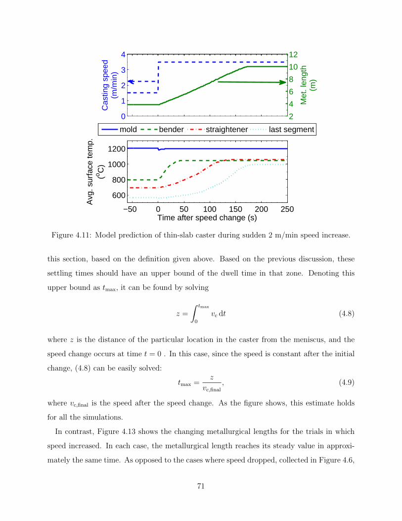
0

1

2

3

4

Cas

ting

spee

d(m

/min

)2

4

6

8

10

12

Met

. len

gth

(m)

−50 0 50 100 150 200 250

600

800

1000

1200


Avg

. sur

face

tem

p.(o C

)


Figure 4.11: Model prediction of thin-slab caster during sudden 2 m/min speed increase.

this section, based on the definition given above. Based on the previous discussion, these

settling times should have an upper bound of the dwell time in that zone. Denoting this

upper bound as tmax, it can be found by solving

z =

∫ tmax

0

vc dt (4.8)

where z is the distance of the particular location in the caster from the meniscus, and the

speed change occurs at time t = 0 . In this case, since the speed is constant after the initial

change, (4.8) can be easily solved:

tmax =z

vc,final

, (4.9)

where vc,final is the speed after the speed change. As the figure shows, this estimate holds

for all the simulations.

In contrast, Figure 4.13 shows the changing metallurgical lengths for the trials in which

speed increased. In each case, the metallurgical length reaches its steady value in approxi-

mately the same time. As opposed to the cases where speed dropped, collected in Figure 4.6,

71

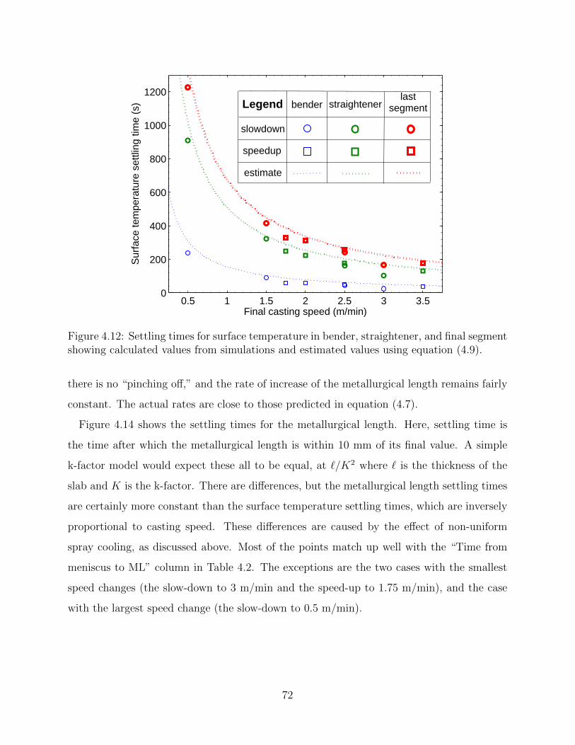
0.5 1 1.5 2 2.5 3 3.50

200

400

600

800

1000

1200

Final casting speed (m/min)

Sur

face

tem

pera

ture

set

tling

tim

e (s

)

lastsegmentstraightenerbender

slowdown

speedup

Legend

estimate

Figure 4.12: Settling times for surface temperature in bender, straightener, and final segmentshowing calculated values from simulations and estimated values using equation (4.9).

there is no “pinching off,” and the rate of increase of the metallurgical length remains fairly

constant. The actual rates are close to those predicted in equation (4.7).

Figure 4.14 shows the settling times for the metallurgical length. Here, settling time is

the time after which the metallurgical length is within 10 mm of its final value. A simple

k-factor model would expect these all to be equal, at `/K2 where ` is the thickness of the

slab and K is the k-factor. There are differences, but the metallurgical length settling times

are certainly more constant than the surface temperature settling times, which are inversely

proportional to casting speed. These differences are caused by the effect of non-uniform

spray cooling, as discussed above. Most of the points match up well with the “Time from

meniscus to ML” column in Table 4.2. The exceptions are the two cases with the smallest

speed changes (the slow-down to 3 m/min and the speed-up to 1.75 m/min), and the case

with the largest speed change (the slow-down to 0.5 m/min).

72

−50 0 50 100 150 2003

4

5

6

7

8

9

10

11


Met

. Len

gth

(m)

0.250.512

Size of speed change(m/min)

Figure 4.13: Metallurgical length during sudden speed increases.

73

0.5 1 1.5 2 2.5 3 3.5140

150

160

170

180

190

Final casting speed (m/min)

Met

. len

gth

settl

ing

time

(s)

slow−downspeed−up

Figure 4.14: Settling times for metallurgical length calculated from simulations.

4.3 Sequential speed changes, and effect of control strategy

The validation case in Section 3.2.4 showed that complicated behavior can occur when the

casting speed changes multiple times without allowing the strand to come to a steady state

in between. In this section, this behavior is examined for the thin-slab Nucor Decatur

caster. Moreover, since Cononline was developed specifically to control the spray cooling

in this caster, additional simulations have been performed to investigate how this behavior

is affected by the spray cooling practice. In these simulations, the casting speed has been

changed from 3.5 to 2.5 m/min and then back, with different amounts of time between the

two speed changes.

The first set of Figures, 4.15 through 4.19 use constant spray water flow rates, as in

the previous section. The caster is 11.2 m long, so at 2.5 m/min it takes approximately

4.5 m for the first speed change to complete. Thus, Figure 4.15, in which 5 minutes pass

between speed changes, shows a change from one steady-state to another, similar to the

figures in Section 4.2. Figure 4.16, in which 4 minutes pass, appears much the same, with

the temperatures and metallurgical length beginning to increase immediately after the speed

74

2

2.5

3

3.5

4

Cas

ting

spee

d(m

/min

)6

7

8

9

10

11

Met

. len

gth

(m)

0 100 200 300 400 500

900

1000

1100

1200


Avg

. sur

face

tem

p.(o C

)


Figure 4.15: Model prediction of thin-slab caster during sequential sudden 1 m/min slow-down and speed-up, with 5 minutes in between speed changes, with constant spray cooling.

increases.

However, Figure 4.17, in which 3 minutes pass, is different. In this figure, the temperature

in the last segment continues to decrease after the speed increases. This is because the

second speed change occurred before steady state was reached after the first speed change. In

Figures 4.18 and 4.19, in which 2 and 1 minute pass respectively, this affects the metallurgical

length as well. The dynamic behavior of the metallurgical length can similarly be understood

as the conflict of these two separate transient behaviors. In Figure 4.15, during the slow-

down, the ML decreases at one speed for the first 120 seconds, and faster afterwards. During

the speed-up, the ML increases at a consistent speed. In Figure 4.19, immediately after the

speed-up, the ML stays approximately constant. In the separate transient behaviors, this

time corresponds to when the slopes of the ML lines are the same size in opposite directions.

Just before the slow-down transient finishes, the ML decreases faster, as it does during the

slow-down. Shortly after, the effect of the slow-down transient is complete, and the ML

increases due to the speed-up alone.

75

2

2.5

3

3.5

4

Cas

ting

spee

d(m

/min

)

6

7

8

9

10

11

Met

. len

gth

(m)

0 100 200 300 400

900

1000

1100

1200

1300


Avg

. sur

face

tem

p.(o C

)



2

2.5

3

3.5

4

Cas

ting

spee

d(m

/min

)

6

7

8

9

10

11

Met

. len

gth

(m)

0 100 200 300 400900

1000

1100

1200

1300


Avg

. sur

face

tem

p.(o C

)



76

2

2.5

3

3.5

4

Cas

ting

spee

d(m

/min

)6

7

8

9

10

11

Met

. len

gth

(m)

0 100 200 300900

1000

1100

1200


Avg

. sur

face

tem

p.(o C

)



2

2.5

3

3.5

4

Cas

ting

spee

d(m

/min

)

6

7

8

9

10

11

Met

. len

gth

(m)

−50 0 50 100 150 200 250 300

1000

1100

1200


Avg

. sur

face

tem

p.(o C

)


Figure 4.19: Model prediction of thin-slab caster during sequential sudden 1 m/min slow-down and speed-up, with 1 minute in between speed changes, with constant spray cooling.

77

Now, Figures 4.20 and 4.21 illustrate two of these cases when the just-presented constant

spray rates are replaced with the “spray-table” open-loop control method to control the

secondary cooling sprays. With this method, the spray rates are chosen based on casting

speed alone. They will decrease as soon as the speed decreases, and increase when the

speed increases. In Figure 4.20, 5 minutes pass, allowing the caster to reach a new steady

state. However, note that the surface temperatures are actually higher in some locations at

the lower speed. This is because the spray rates were not exactly tuned to give constant

temperatures at all casting speeds. Also note that the temperature in the bender and

straightener overshoot before coming to steady state. This is because the sprays change

immediately when the speed changes, and do not account for the dwell time of the material

in the caster. This is also the reason why the metallurgical length has inflection points both

during the slow-down and speed-up. The transient behavior of the steel and the transient

behavior of the sprays conflict with each other. Thus, in Figure 4.21, with only 1 minute

between speed changes, there are overlapping transients of not only the speed changes, but

the spray changes as well. This causes complicated behavior in the metallurgical length and

temperature profile histories.

Figures 4.22 and 4.23 show the same two casting speed cases, but using the surface tem-

perature PI controller described in Section 2.4.3. As shown in 4.22, the PI controller gives

much more consistent temperatures when moving from one steady-state to the other, and

almost linear metallurgical length movement. The PI controllers are responding directly to

the heat transfer dynamics of the steel, as modelled by Consensor. Even with only 1 minute

between speed changes, the performance is equally good, as seen in Figure 4.23. The tem-

perature in the bender does vary more than the temperature in other segments, by design.

For quality reasons, the temperature in each slice should not change drastically through the

bender. This is achieved by tuning the PI gains in that spray zone to sacrifice temperature

tracking for smoothly varying water flow rates.

With the spray control keeping constant surface temperatures, the metallurgical length

still moves around about 2.5 m in these examples. This has significant importance to product

quality, as soft reduction in the caster needs to be located at final solidification. Machines

with dynamic soft reduction can change roll spacing to account for this, necessitating a

78

2

2.5

3

3.5

4

Cas

ting

spee

d(m

/min

)6

7

8

9

10

11

Met

. len

gth

(m)

0 100 200 300 400 500 600

1000

1100

1200


Avg

. sur

face

tem

p.(o C

)


Figure 4.20: Model prediction of thin-slab caster during sequential sudden 1 m/min slow-down and speed-up, with 5 minutes in between speed changes, with speed-based spray coolingcontrol.

2

2.5

3

3.5

4

Cas

ting

spee

d(m

/min

)

6

7

8

9

10

11

Met

. len

gth

(m)

−50 0 50 100 150 200 250 300

1000

1100

1200


Avg

. sur

face

tem

p.(o C

)


Figure 4.21: Model prediction of thin-slab caster during sequential sudden 1 m/min slow-down and speed-up, with 1 minute in between speed changes, with speed-based spray coolingcontrol.

79

2

2.5

3

3.5

4

Cas

ting

spee

d(m

/min

)6

7

8

9

10

11

Met

. len

gth

(m)

0 100 200 300 400 500 600

1000

1100

1200


Avg

. sur

face

tem

p.(o C

)


Figure 4.22: Model prediction of thin-slab caster during sequential sudden 1 m/min slow-down and speed-up, with 5 minutes in between speed changes, with temperature-based PIspray cooling control.

2

2.5

3

3.5

4

Cas

ting

spee

d(m

/min

)

6

7

8

9

10

11

Met

. len

gth

(m)

−50 0 50 100 150 200 250 300

1000

1100

1200


Avg

. sur

face

tem

p.(o C

)


Figure 4.23: Model prediction of thin-slab caster during sequential sudden 1 m/min slow-down and speed-up, with 1 minute in between speed changes, with temperature-based PIspray cooling control.

80

real-time model like Consensor to accurately predict where soft reduction should occur.

Another feature of the figures is that the metallurgical length slightly undershoots its final

value on the slow-down, and slightly overshoots on the speed-up. This is the natural trade-

off between temperature tracking and metallurgical length tracking goals. If this overshoot

extends out of containment, a catastrophic whale event would occur. Zheng suggested an

ad hoc method of adjusting the temperature setpoints to prevent these whales in [53]. How-

ever, a preferable solution would be to have a control method that simultaneously regulated

shell thickness and surface temperature. This, however, is a significantly more complicated

problem, as it requires controlling the entire distributed, nonlinearly evolving, temperature

profile of the strand.

81

Part II

Developing a control theory for

nonlinear PDEs describing

solidification

82

CHAPTER 5

CONTROL LAW FROM TEMPERATURE-BASEDLYAPUNOV FUNCTIONAL

The key aspects of the control system presented in the previous part are illustrated in Fig-

ure 5.1. The control system design was focused on the inability to measure the temperature

of the steel in the caster, and the most sophisticated part of the system was the model acting

as an open-loop estimator of the process. The controlled input to the process is the flow

rates of the water cooling sprays in the caster. The controller itself was a simple bank of

SISO PI controllers, and the only error considered was at the surface of the steel, in part

due to the difficulty of analyzing the nonlinear PDE governing the process. This represented

a great improvement over existing control systems, but is not fully satisfactory. This part

presents control algorithms for controlling the entire temperature of the material, surface

and internal. To do so, however, the complexity of the system must at first be reduced,

by simplifying the boundary condition (actuator) and material models to the more basic

nonlinear Stefan problem PDE discussed in Section 1.4.2.

This chapter is based on the paper [24], presented at the Conference on Decision and

Control in December 2010. The goal is to stabilize the solution to the Stefan problem relative

to a reference solution. The reference is assumed to be safe and provide good metallurgical

quality under nominal conditions, so that the process goals are met by reducing the reference

error to zero. The key tool is a Lyapunov functional on solutions of the Stefan problem with

a moving boundary. This allows for the construction of a control law that stabilizes the

error, and shows convergence of the error to zero asymptotically. It will turn out that this

procedure gives a control law that is not realistically implementable. These results will be

improved on in the next chapter, and the reader should feel free to skip ahead. The results

here are included for the sake of completeness.

In Section 5.1, the necessary assumptions are given and the partial differential equations for

83

Figure 5.1: Simplified block diagram

the error are introduced. In Section 5.2, a control law for the Neumann boundary condition

of the Stefan problem is provided, and the associated proof of convergence. In Section 5.3,

simulation results are presented that support the theorems and conjectures made in this

section.

5.1 The two–phase Stefan Problem

5.1.1 Assumptions

For the convergence proof, the following assumptions on the initial conditions are needed:

(A1) 0 < s0 < `, T0(s0) = Tf , T0(x) < Tf for 0 ≤ x < s0 and T0(x) ≥ Tf for s0 ≤ x ≤ `.

(A2) T0 (x) is continuous on the interval [0, `] and infinitely differentiable inside, except at

s0.

The assumptions, respectively, ensure that the equations are well defined at t = 0 and that

solutions have sufficient regularity. Furthermore, only the case in which ε < s(t) < ` − ε

for some ε > 0, is considered, that is when the slice is neither fully solid nor liquid and the

Stefan problem is well defined. If this is not true, the problem is linear and may be dealt

with using known distributed parameter control methods, e.g. those in [54].

84

5.1.2 Reference system and error

Assume that a known reference temperature T (x, t) and solidification front position s(t) ,

have been determined that are the solutions to (1.7)-(1.10) under known reference control

input u(t) with initial conditions T (x, 0) = T0 and s(0) = s0 satisfying assumptions (A1)

and (A2). This reference temperature profile should satisfy the metallurgical goals and

constraints of the process, and could, for example, be calculated for the continuous caster

via the optimization methods of [3, 4] or the inverse methods of [5, 6, 7]. That is, matching

the reference temperature should result in safe operation and good quality steel. One more

assumption on the reference profile is required:

(A3) ˙s(t) ≥ 0 for all t ≥ 0

Denote the reference errors as T (x, t) = T (x, t) − T (x, t) , and s(t) = s(t) − s(t) . Also,

denote the addition to the boundary heat flux as u(t) = u(t)− u(t) . Subtracting the PDEs

yields

Tt(x, t) = aTxx(x, t) , x ∈ (0, `)− s, s . (5.1)

T (0, t) = u(t) T (`, t) = 0 (5.2)

Also, since solutions to (1.7) are twice spatially differentiable away from the solidifica-

tion front, they must have continuous first spatial derivatives. Thus, if s(t) 6= s(t) , then

Tx(s+(t) , t) = Tx(s−(t) , t) , and so

s(t) = b(Tx(s−(t) , t

)− Tx

(s+ (t) , t

)). (5.3)

Similarly,

˙s (t) = −b(Tx(s−(t) , t

)− Tx

(s+ (t) , t

)). (5.4)

From here on, notation will be simplified for clarity and space, using T (x) to represent

T (x, t) , or omitting both arguments altogether.

85

5.2 Control law

The main result of this chapter is stated as follows:

Theorem 5.2.1. Let the system (1.7)–(1.10) be controlled such that

u(t) = u(t)− 1

T (0) + Txx(0)

[Tx(x)

(T (x) + Txx(x)

)∣∣∣s+s−

+ Tx(x)(T (x) + Txx(x)

)∣∣∣s+s−

+1

2as(t) T 2

x (x)∣∣∣s+s−

+1

2a˙s(t) T 2

x (x)∣∣∣s+s−

] (5.5)

where the initial conditions satisfy (A1) and (A2), and the reference solidification front

position satisfies (A3). Then the reference error T (x, t) converges uniformly to 0 as t→∞.

Proof. Consider the Lyapunov functional

V(T)

:=1

2

∫ `

0

(T 2 + T 2

x

)dx

=1

2

[∫ s1

0

(T 2 + T 2

x

)dx+

∫ s2

s1

(T 2 + T 2

x

)dx+

∫ `

s2

(T 2 + T 2

x

)dx

],

(5.6)

where s1 := min s, s and s2 := max s, s . Note that V(T)

is equivalent to the square of

the Sobolev norm, ∥∥∥T∥∥∥1,2

:=∥∥∥T∥∥∥

2+∥∥∥Tx∥∥∥

2,

in the sense that1

2

∥∥∥T∥∥∥1,2

2

≥ V(T)≥ 1

4

∥∥∥T∥∥∥1,2

2

. (5.7)

Since solutions of the Stefan problem are continuous and twice differentiable except at

the boundary, the first weak derivative exists and such solutions are in the Sobolev space

H1(0, `) .

Assuming that s(t) 6= s(t) , and ignoring the degenerate case for now, the time derivative

86

of (5.6) is given by:

V(T , t)

=1

2

(T 2(s−1)

+ T2

x

(s−1))s1 +

1

2

[(T 2(s−2)

+ T2

x

(s−2))s2

−(T 2(s−1)

+ T2

x

(s−1))s1

]− 1

2

(T 2(s−2)

+ T2

x

(s−2))s2

+

∫ s1

0

(T Tt + TxTxt

)dx +

∫ s2

s1

(T Tt + TxTxt

)dx+

∫ `

s2

(T Tt + TxTxt

)dx.

Inserting the PDE from (5.1) yields:

V(T , t)

= − 1

2s1

(T 2 (x) + T

2

x (x))∣∣∣s+1

s−1

− 1

2s2

(T 2 (x) + T

2

x (x))∣∣∣s+2

s−2

+

∫ s1

0

(T Txx + TxTxxx

)dx+

∫ s2

s1

(T Txx + TxTxxx

)dx

+

∫ `

s2

(T Tx + TxTxxx

)dx.

Note that the expression above contains the third spatial derivative. Since T and T are

solutions to the parabolic heat equation on the time-varying domains (0, s) ∪ (s, `) and

(0, s) ∪ (s, `), respectively, they will be at least three times differentiable, as shown in a

techical lemma in [24]. Therefore, T will also have the third spatial derivative except at the

boundary points.

Now, integrating by parts,

V(T , t)

= − 1

2s1

(T 2 (x) + T

2

x (x))∣∣∣s+1

s−1

− 1

2s2

(T 2 (x) + T

2

x (x))∣∣∣s+2

s−2

+ a(T Tx + TxTxx

)∣∣∣s10− a

∫ s1

0

(T 2x + T 2

xx

)dx

+ a(T Tx + TxTxx

)∣∣∣s2s1− a

∫ s2

s1

(T 2x + T 2

xx

)dx

+ a(T Tx + TxTxx

)∣∣∣`s1− a

∫ `

s1

(T 2x + T 2

xx

)dx.

87

Then, applying the boundary conditions from (1.8) and combining like terms gives

V(T , t)

= − a∫ `

0

(T 2x + T 2

xx

)dx− au (0)

(T (0) + Txx (0)

)− a Tx (x)

(T (x) + Txx (x)

)∣∣∣s+1s−1

− a Tx (x)(T (x) + Txx (x)

)∣∣∣s+2s−2

− 1

2s1 T

2

x (x)∣∣∣s+1s−1

− 1

2s2 T

2

x (x)∣∣∣s+2s−2

.

Hence, if the control u (t) satisfies (5.5), then

V(T , t)

= −a∫ `

0

(T 2x + T 2

xx

)dx =: W

(T)≤ 0. (5.8)

Now, consider the degenerate case, in which s (t) = s (t) for some time interval of length

greater than zero. This means T (s (t) , t) = 0 in this interval, and since the boundaries move

as governed by (1.10),

Tx(s−)− Tx

(s+)

= Tx(s−)− Tx

(s+)

⇒ Tx(s+)

= Tx(s−)

=: T (s) .

Then (5.5) simplifies to

u (t) = u (t)− 2Tx (s)

T (0) + Txx (0)Txx (x)

∣∣∣s+s−.

Using these relationships and (5.1), the time derivative of (5.6) can be calculated, which in

the degenerate case only has a single boundary. After integrating by parts,

V(T , t)

= −a∫ `

0

(T 2x + T 2

xx

)dx+ aTx (s) Txx (x)

∣∣∣s+s−. (5.9)

If Tx (s) = 0, then (5.8) clearly holds. If Tx (s) > 0, then for all ε > 0 sufficiently small,

T (s+ ε) > 0. If Txx (s+) > 0, then by (5.1), Tt (s+ ε) > c > 0 for all ε > 0 sufficiently

small. This means T (s (t) + ε, t+ δ) > 0 for all δ > 0 sufficiently small. But, by assumption

88

(A3), within the degenerate time interval,

s (t+ δ) = s (t+ δ) > s (t) = s (t)⇒ s (t+ δ) = s (t) + ε

for some ε > 0. This means, taking δ small enough,

0 = T (s (t+ δ) , t+ δ) = T (s (t) + ε, t+ δ) > 0.

By contradiction, then, Txx (s+) ≤ 0. Similarly, Txx (s−) ≥ 0. Therefore,

aTx (s) Txx (x)∣∣∣s+s−≤ 0

and (5.8) follows from (5.9). The same argument holds under reversed signs in the case

Tx (s) < 0. Thus, in the degenerate case, under the given control law, the estimate (5.8) is

still valid.

As an immediate conclusion of (5.7) and (5.8), under this control law the reference error T

is bounded in the H1 (0, `) Sobolev norm. The proof is completed by applying an invariance

principle for general evolution equations from [55], summarized in Appendix B.2. Define the

spaces X := H1 (0, `) and Y := C0 (0, `), and let f (x) be an admissible initial value for the

reference error. That is, f (x) = T0− T0 where T0 and T0 satisfy assumptions (A1) and (A2).

Define G := γ (f) :=⋃t≥0

S (t)f where S (t)f is the solution to the error equations under the

given control law. Since solutions to the Stefan problem are continuous and piecewise-C2,

G ⊂ X , and by Lemma B.2.1, X is compactly embedded in Y . Therefore, G is compactly

embedded in Y and, as noted above, G is X -bounded. Define

V (y) :=

∫ `

0

(T 2 + T 2

x

)dx

and

W (y) :=

∫ `

0

(T 2x + T 2

xx

)dx

to be, respectively, the extensions of V and W (defined in (5.8)) to ClYG. the closure of G

89

in the supremum norm. Since functions in G will be twice differentiable almost everywhere,

both of these functionals are well defined, positive semi-definite, and lower semi-continuous

on ClYG. Thus, all the conditions of Theorem 6.3, p. 195, in [55] are met, giving the following

result:

limt→∞

dy (S (t) f,M3) = 0 (5.10)

where

M3 :=y ∈ ClYG : W (y) = 0

. (5.11)

In general, M3 :=T (x) : Tx (x) ≡ 0 ≡ Txx (x)

, that is T (x) = T (x) + C for some

constant C. So, consider any constant element T (x) ≡ C in G. If C 6= 0, then s 6= s, but

since T is continuously differentiable except at s,

Tx(s+)

= Tx(s+)

= Tx(s−)

= Tx(s−).

Then by (1.10),

˙s = −b(Tx(s+)− Tx

(s−))

= 0.

This contradicts assumption (A3). This means that M3 ∩ G = 0, and since M3 ⊂ ClYG,

M3 = 0. Therefore, (5.10) is equivalent to

limt→∞

∥∥∥T (x, t)∥∥∥∞

= 0.

There are two important points to make about Theorem 5.2.1. First, it does not follow

from Theorem 5.2.1 that the solidification front position converges as well. If the temper-

ature gradient in the reference profile is small, the solidification front position error may

be arbitrarily large for small temperature errors. For practical applications, though, this

gradient is not small, and the solidification front converges close to the reference position as

illustrated in the simulations in Section 5.3.

Second, the well-posedness of the 1-D Stefan problem has been examined in depth, e.g.

in [30, 31, 32], typically requiring boundedness of the boundary conditions and their time

derivatives. The control law (5.5) may be unbounded. In the simulations, some regularity is

90

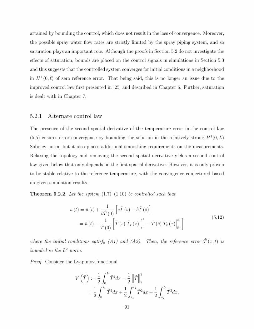
attained by bounding the control, which does not result in the loss of convergence. Moreover,

the possible spray water flow rates are strictly limited by the spray piping system, and so

saturation plays an important role. Although the proofs in Section 5.2 do not investigate the

effects of saturation, bounds are placed on the control signals in simulations in Section 5.3

and this suggests that the controlled system converges for initial conditions in a neighborhood

in H1 (0, `) of zero reference error. That being said, this is no longer an issue due to the

improved control law first presented in [25] and described in Chapter 6. Further, saturation

is dealt with in Chapter 7.

5.2.1 Alternate control law

The presence of the second spatial derivative of the temperature error in the control law

(5.5) ensures error convergence by bounding the solution in the relatively strong H1(0, L)

Sobolev norm, but it also places additional smoothing requirements on the measurements.

Relaxing the topology and removing the second spatial derivative yields a second control

law given below that only depends on the first spatial derivative. However, it is only proven

to be stable relative to the reference temperature, with the convergence conjectured based

on given simulation results.

Theorem 5.2.2. Let the system (1.7)–(1.10) be controlled such that

u (t) = u (t) +1

bT (0)

[sT (s)− ˙sT (s)

]= u (t)− 1

T (0)

[T (s) Tx (x)

∣∣∣s+s−− T (s) Tx (x)

∣∣∣s+s−

] (5.12)

where the initial conditions satisfy (A1) and (A2). Then, the reference error T (x, t) is

bounded in the L2 norm.

Proof. Consider the Lyapunov functional

V(T)

:=1

2

∫ L

0

T 2dx =1

2

∥∥∥T∥∥∥2

2

=1

2

∫ s1

0

T 2dx+1

2

∫ s2

s1

T 2dx+1

2

∫ L

s2

T 2dx,

91

where s1 := min s, s and s2 := max s, s. As in Theorem 5.2.1, take the time derivative

and integrate by parts, substituting in the PDEs and boundary conditions where appropriate.

The result is

V(T , t)

= −a∫ L

0

T 2xdx− au (t) T (0)

− a Tx (x)∣∣∣s+1s−1

T (s1)− a Tx (x)∣∣∣s+2s−2

T (s2)

= −a[∫ L

0

T 2xdx− u (t) T (0) +

1

bsT (s)− 1

b˙sT (s)

].

If the control law satisfies (5.12),

V(T , t)

= −a∫ L

0

T 2xdx ≤ 0. (5.13)

In the degenerate case s = s, control law (5.12) reduces to u = u. Again taking the time

derivative and integrating by parts gives (5.12), where the boundary terms drop out because

u = 0 and T (s) = T (s) = 0. Therefore, V(T)

, and consequently∥∥∥T∥∥∥

2, is bounded over

time.

5.3 Simulation results

The following simulation results, from [24], use the parameters in Table 1. These are based

on the thermal properties of ULC (ultra-low carbon) steel. The initial conditions are shown

in Figure 5.2. As discussed above, the simulations employ an enthalpy-based method to

model solidification, rather than an actual moving boundary. The controlled simulations

were found to be very noisy, as seen in Figure 5.4c, and a hard bound was put on the

permitted control values. This also better corresponds to the continuous casting process

constraints, as heat fluxes below zero and above the maximum available by the water spray

cooling system cannot be achieved.

Figure 5.3 shows the behavior of the system under open-loop control with u (t) = u (t)

for all t ≥ 0. In this case, the reference errors in both temperature and solidification front

92

Table 5.1: Thermodynamic properties used in section 5.3

Symbol Description Valuea thermal diffusivity 6.051× 10−6 W/m · Kb Stefan condition constant 1.496× 10−8 m2/K · sTf melting temperature 1782 K` half-thickness of strand 0.05 m

Figure 5.2: Initial condition for simulations in Section 5

93

position appear to converge to constant, non-zero values. This approximates the current

spray cooling state-of-the-art in most continuous casters, in which spray practices do not

account for changes in superheat or mold heat removal.

Figure 5.4 shows simulation results using control law (5.5). Although Theorem 5.2.1 does

not demonstrate convergence for the solidification front, the simulated solidification front

position does converge to the reference. Similarly, although convergence for the saturated

control laws was not proven, the simulations demonstrate that the bounded control values

do allow for good convergence. Still, the lack of bounded control output is a serious concern

regarding this result.

Figure 5.5 shows simulation results using control law (5.12). Once again, the behavior in

simulation is better than the proven in the theorem. Theorem 5.2.2 only ensures bounded

temperature error in the L2 norm, but the temperature and solidification front both appear

to be converging to the reference. However, despite the lack of second derivative in the

control denominator, the control is not any less noisy in Figure 5.5c than in Figure 5.4c.

It is very important to note that these simulation results are very sensitive to the simulation

parameters – both physical and numerical.

5.4 Summary

As of now, the designed controller has the form of the block diagram in Figure 5.6. The

details of the math are in Figure 5.7. Compared with the control system of the previous part,

in Figure 5.1, this is obviously a greatly simplified setting. Only a single slice of the caster

is considered, and full-state feedback of the slice temperature is required. However, this was

the first, to my knowledge, example of feedback control of the distributed temperature in

solidification, governed by a non-linear PDE. The techniques first presented in [24] can, as

will be shown in the following chapters, be extended to produce a more reasonable control

law. Chapter 6 focuses on dealing with the issue of unbounded and non-smooth control seen

in Figures 5.4c and 5.5c. Chapter 7, adds back in some of the missing complexity to the

system model, while maintaining temperature convergence.

94

(a) Temperature error T (x, t)

(b) Solidification front s(t)

Figure 5.3: Simulation of system (1.7)-(1.10) with initial condition mismatch and no controladjustment

95



(c) Boundary control u(t)

Figure 5.4: Simulation of system (1.7)-(1.10) with initial condition mismatch and controllaw (5.5)

96



(c) Boundary control u(t)


97

Figure 5.6: Overview block diagram for Chapter 5.

Figure 5.7: Block diagram showing equations from Chapter 5.

98

CHAPTER 6

CONTROL LAW FROM ENTHALPY-BASEDLYAPUNOV DESIGN

I claim that the key weakness that led to the unbounded control is actually conceptual.

The previous attempt used the temperature, because it was the output of interest, for the

Lyapunov functional used for controller design. Instead, the design should have focused on

the enthalpy. As discussed in Section 1.4.1, the enthalpy is the actual energy of interest in

the problem. In [25], the control law was re-designed based on this principle, and the results

are summarized in this chapter. This method produced more well-behaved dynamics in the

controlled system, but required another slight simplification of the problem.

6.1 Modeling simplification: the one-phase Stefan problem

In actual casting conditions, the temperature in the liquid is negligible. A typical superheat

(the difference between the initial temperature in the liquid and the melting temperature) is

only around 25C. In comparison, the average surface temperature of the steel in the caster

is around 500C less than the melting temperature. Moreover, due to fluid flow in the liquid,

the temperature in the liquid reaches steady state much more quickly than conduction alone

would achieve. Hence, a common modeling assumption for this problem is to assume the

initial temperature in the liquid is uniformly equal to the melting temperature, Tf .

This reduces the dynamics of the problem to only those of the solid phase. However, for

ease of notation and calculation, this chapter will continue to use the PDE (1.7)-(1.10), with

the following assumption:

(A4) The initial conditions satisfy: 0 < s0 < `, T0 (x) < Tf and is non-decreasing for all

0 ≤ x < s0, and T0 (x) = Tf for all x ≥ s0, and are piece-wise smooth.

Also, assume the control input u (t) is bounded:

99

(A5) inf u (t) ≥ 0 and supu (t) <∞.

These assumptions are physically sensible for the target application. Castings solidify from

the outside in, and since they are at high temperatures there is always some minimum cooling

at the surface due to radiation and natural convection. Whenever possible, conditions will

be given that ensure the assumptions are satisfied. As in the previous chapter, only the case

when 0 < s < ` is considered.

The reference temperature T (x, t) and solidification front position s(t), and the reference

errors T (x, t) and s(t) are defined as in Chapter 5. In particular, the error PDEs still satisfy

(5.1)–(5.4).

As they are continuous and piecewise continuously differentiable, T , T , and T are all

in the Sobolev space H1(0, `) at all times. Continue to denote, when needed, s1(t) =

min s(t) , s(t) and s2(t) = max s(t) , s(t). As in the previous section,notation will be

simplified by dropping the argument(s) for most terms.

6.2 Preliminaries and notation

If the solution (T, s) to the PDE (1.7)-(1.10) satisfies assumptions (A4)–(A5), a few facts

immediately follow. First, T0 (x) < Tf and is non-decreasing for all 0 ≤ x < s (t), which

in turn implies s (t) ≥ 0 for all t ≥ 0. For the single-phase Stefan problem, T (x) ≡ 0

when s2 ≤ x ≤ `. Since (1.7) is parabolic on the subdomains, if (A6) holds then Tx is

uniformly bounded by a constant depending on the initial condition and bounds on u. (See,

e.g., Theorem 11.1 from Section III.11, p. 211 of [29].) By (1.10), this means that the

solidification front speed is bounded, i.e.

0 ≤ vmin ≤ s ≤ vmax <∞ (6.1)

Also, as a consequence of the version of Poincares inequality given in [54] (Lemma 2.1,

p. 17), there is a bound on ‖T‖2:

∫ `

0

T 2 dx ≤ 2T 2 (s) + 4`2

∫ `

0

T 2x dx = 2T 2

f + 4`2

∫ `

0

T 2x dx. (6.2)

100

That is, both T and Tx are bounded in the L2 (0, `) norm, and hence T is bounded in the

Sobolev space H1 (0, `). Similarly, Agmons Inequality (Lemma 2.4, p. 20, ibid) ensures that

|T | is also uniformly bounded.

Similar to the discussion of enthalpy in Chapter 1, let the “enthalpy function” η (T ) be

defined as:

η(T ) :=

1aT, if T < Tf

1aT + 1

b, if T ≥ Tf

. (6.3)

This is not the same as the physical enthalpy, defined as (1.1) in Section 1.4.1, but it is dif-

ferent only by multiplication by a constant. However, this form will simplify the calculations

to follow. Hence, the uncommon notation of η is used for this function. In this section, the

notation

η := η(T )− η(T)

is used for the difference in enthalpy and

H :=

∫ `

0

η dx =1

a

∫ `

0

T dx− 1

bs, (6.4)

for the total difference. Taking the time derivative of this value, and using the fact that T

is continuous,

d

dtH =

d

dt

(1

a

∫ `

0

T dx− 1

bs

)=

1

a

∫ `

0

Tt dx− 1

b˙s

.

Using equations (5.1)-(5.4),

d

dtH =

∫ `

0

Txx −1

bs+

1

b˙s

= Tx

∣∣∣s−10

+ Tx

∣∣∣s−2s+1

+ Tx

∣∣∣`s+2

+ Tx

∣∣∣s+s−

+ Tx

∣∣∣s+s−

= −Tx (0) + Tx (`) = −u.

(6.5)

101

6.3 Control law

With these estimates in mind, the main result of this section can be stated:

Theorem 6.3.1. Suppose the initial conditions satisfy assumption (A4), the reference tem-

perature profile satisfies assumptions (A4) and (A5), the boundary condition satisfies the

control law

u (t) = u (t) +KH (t) , (6.6)

and the closed-loop system satisfies assumptions (A5). Then the reference temperature error

T converges asymptotically to 0 uniformly over the domain, and the interface position error

s converges to 0 asymptotically as well.

Proof. In light of (6.5), if the control law (6.6) is used,∣∣∣H∣∣∣ and |u| are exponentially de-

creasing. As noted above, if all assumptions are satisfied, T and T , and consequently also

T are bounded in H1 (0, `) over time. Then, by the definition of H in (6.4), |s| must also be

bounded.

Similar to the Chapter 5, the proof here will be an application the infinite-dimensional

invariance principle from [55], summarized in Appendix B. Consider the Lyapunov functional

candidate

V(T)

:=1

2

∫ `

0

T 2 dx− a

bTf (s+ s) + 2

a

bTf`

on the state space of the error system,(T , s

)∈ H1 (0, `) × R. This function is clearly

continuous on that space, and non-negative on trajectories of the system.

Taking the time derivative of the first term,

d

dt

1

2

∫ `

0

T 2 dx =1

2

d

dt

[∫ s

0

T 2 dx+

∫ s

s

T 2 dx+

∫ `

s

T 2 dx

]=

∫ s

0

T Tt dx+

∫ s

s

T Tt dx+

∫ `

s

T Tt dx.

(6.7)

102

Then, applying the PDE (1.7), and integrating by parts,

d

dt

1

2

∫ `

0

T 2 dx = a

∫ s1

0

T Txx dx+ a

∫ s2

s1

T Txx dx+ a

∫ `

s2

T Txx dx

= aT Tx

∣∣∣s−10− a

∫ s1

0

T 2x dx+ aT Tx

∣∣∣s−2s+1

− a∫ s2

s1

T 2x dx+ aT Tx

∣∣∣`s+2

− a∫ `

s2

T 2x dx

= −aT (0) Tx (0)− aT Tx

∣∣∣s+s−− aT Tx

∣∣∣s+s−

+ aT (`)Tx (`)− a∫ `

0

T 2x dx.

Applying the boundary conditions from (1.8) and the relationships (5.3) and (5.4),

d

dt

1

2

∫ `

0

T 2 dx = −aT (0) u− a∫ `

0

T 2x dx+

a

bT (s) s− a

bT (s) ˙s (6.8)

Differentiating the second term using gives

d

dt

a

bTf s =

a

bTf (s+ ˙s) . (6.9)

Combining (6.8) and (6.9),

d

dtV(T)

= −aT (0) u− a∫ `

0

T 2x dx+

a

b

(T (s)− Tf

)s− a

b

(T (s) + Tf

)˙s

= −aT (0) u− a∫ `

0

T 2x dx− a

b

(T (s) s+ T (s) ˙s

).

(6.10)

It was already noted that |u| decreases exponentially, and

∣∣∣T (0)∣∣∣ =

∣∣∣T (0)− T (`)∣∣∣ =

∣∣∣∣∫ `

0

Tx dx

∣∣∣∣ ≤ √`∥∥∥Tx∥∥∥2

(6.11)

where the final inequality follows from that of Cauchy-Schwarz. Thus, the first term is

exponentially decreasing. Under the assumptions, both s and ˙s are positive and bounded

below, as discussed above. Since the temperatures are bounded, choosing an appropriate

temperature scale ensures T (s) and T (s) are also non-negative. So, after enough time,

d

dtV (t) ≤ −a

∫ `

0

T 2x dx

103

Then, applying the Poincare inequality given in [54] (Lemma 2.1, p. 17),

−a∫ `

0

T 2xdx ≤ −

a

4`2

∫ `

0

T 2 dx+ 2T 2 (`)

= − a

4`2

∫ `

0

T 2 dx := −W(T).

The infinite dimensional invariance principle can now be applied. Using the notation of

[55] and Appendix B, denote X to be H1 (0, `)×R, the state space of the problem, and Y to

be C0 (0, `)× R. Denote W and V to be the extensions of W and V respectively to Y . As

discussed in Appendix B, by application of the Rellich-Kondrakov theorem (Theorem 5.5,

p. 269 in [56]) and the Ascoli-Arzela criterion (Appendix C.7, p. 635, ibid), X can be shown

to be compactly embedded in Y . As noted above, the trajectories of the error system are

bounded in the space X . All conditions of the theorem are met, and therefore all trajectories

of the system converge to the set

M3 ⊂y ∈ Y : W (y) = 0

=T ≡ 0

in the Y-norm. That is, T converges to 0 uniformly.

Then, since both T and∣∣∣H∣∣∣ converge to 0, according to the definition (6.4), s must

converge to 0 as well.

6.4 Discussion and Simulation Results

The main weakness of this result lies in the applicability of the assumptions. Assump-

tion (A4) depends only on the initial conditions, and is entirely reasonable. Assumption (A5)

can be satisfied by choosing the controller gain k sufficiently small. For example,

K <inf u

H (t = 0)

will ensure that assumption (A5) holds on u. This gain can be further adjusted to limit the

amount of control actuation, at the trade-off of reducing the rate of convergence.

104

Table 6.1: Thermodynamic properties used in section 6.

Symbol Description Valuea thermal diffusivity 2.27× 10−5 W/m · Kb Stefan condition constant 4.13× 10−8 m2/K · sTf melting temperature 1811 K` half-thickness of strand 0.2 mu constant reference input 3000 K/m

Also, as in Chapter 5, the proof above assumes that 0 < s(t) < `. In in the alternate

cases, s(t) = 0 or s(t) = `, the system is linear, and can be controlled using linear methods.

The conclusion, that the temperature error converges uniformly to 0, will still hold, but this

is not a satisfying result. For certain initial errors and reference profiles, the temperature

error may not converge very closely before solidification is completed. In general, as the

speed ˙s of the reference solidification front speed gets smaller, the temperature and interface

position errors will converge closer to 0 before the material is completely solidified.

A stronger result would be to guarantee the rate of convergence, but I am currently unable

to prove this mathematically. There is, however, simulation evidence that this is the case.

Figure 6.2 show a simulation of this control algorithm. The actual system (T, s) is given a

different initial condition than the reference system(T , s

). The specific initial conditions

used are shown in Figure 6.1, and the rest of the simulation parameters are given in Table

6.1.

Due to the spatial discretization, the location of the interface s has some inherent uncer-

tainty that can lead to numerical noise in control law (6.6). Since the simulation method

used is based on the calculated enthalpy at each node, this was used directly in the control

calculations instead. This ensures the control response, seen in Figure 6.2c, does not spike

whenever the estimated interface position passes a node.

In this simulation, the reference temperature and interface position errors, in Figures 6.2a

and 6.2b, respectively, are clearly converging exponentially fast. Further simulation evidence

of this exponential convergence is given in Chapter 9.

Finally, note that the proof was only specific to the single-phase Stefan problem in applying

Agmons and Poincares Inequalities, e.g. in (6.11), which required that T (`) = 0, and in

105

0 0.01 0.02 0.03 0.04 0.051760

1770

1780

1790

1800

1810

1820

distance from surface, x (m)

initi

al te

mpe

ratu

re, T

0 (K

)

referenceactual

Figure 6.1: Initial condition for simulations in Chapter 6

106

0

1000

2000

00.05

0.10.15

0.2

−20

−10

0

10

20

time, t (s)distance from

strand surface, x (m)

refe

renc

ete

mpe

ratu

re e

rror

(K

)


0 500 1000 1500 20000

0.05

0.1

0.15

0.2

time, t (s)

solid

ifica

tion

fron

tpo

sitio

n, s

(m

)

referencestate−feedback control


0 500 1000 1500 20001000

1500

2000

2500

3000

3500

4000

time, t (s)

Neu

man

n bo

unda

ryco

ntro

l, u

(K/m

)

referencestate−feedback

(c) Boudary control u(t)


107

using the estimate (6.1) to ensure negative definiteness of the Lyapunov functional time

derivative. The former is easily dealt with by using a weaker bound on∥∥∥T∥∥∥

∞based on

compactly embedding H1 (0, `) into C0 (0, `), as described above. The inequality (6.1) is

still usually true for the two-phase Stefan problem, but it is difficult to determine exact

conditions on the inputs and initial conditions that ensure the condition holds. Currently,

the best that can be proven for the two-phase Stefan problem is the following:

Corollary 6.4.1. Suppose the system satisfies the conditions of Theorem 6.3.1, with the

exception that T0 (x) > Tf is allowed in the range s0 < x ≤ `, and a similar condition on the

reference. Then, if both s ≥ 0 and ˙s ≥ 0 for the entire time, the reference temperature error

converges to 0 in the uniform norm, and the interface position error converges to 0 as well.

6.5 Summary

Figure 6.3 shows a block diagram for the control law developed in this chapter, with equations

in the block diagram in Figure 6.4. There is little substantive difference between this one

and the block diagrams for the previous chapter, Figures 5.6 and 5.7, with the control law

being the major difference. The governing model is also slightly simpler. This is not a

major weakness, as the simplifying assumption is actually quite appropriate for the intended

application, which will be backed up by more sophisticated simulations in the final part of

this dissertation. The major change to the controller is changing the control law to use

enthalpy rather than temperature. Enthalpy cannot be directly measured, but temperature

and enthalpy have a nonlinear but static relation, as shown in the block diagrams by the

function (6.3). After this one complication, the actual control law can be greatly simplified,

yet produce much better performance.

108

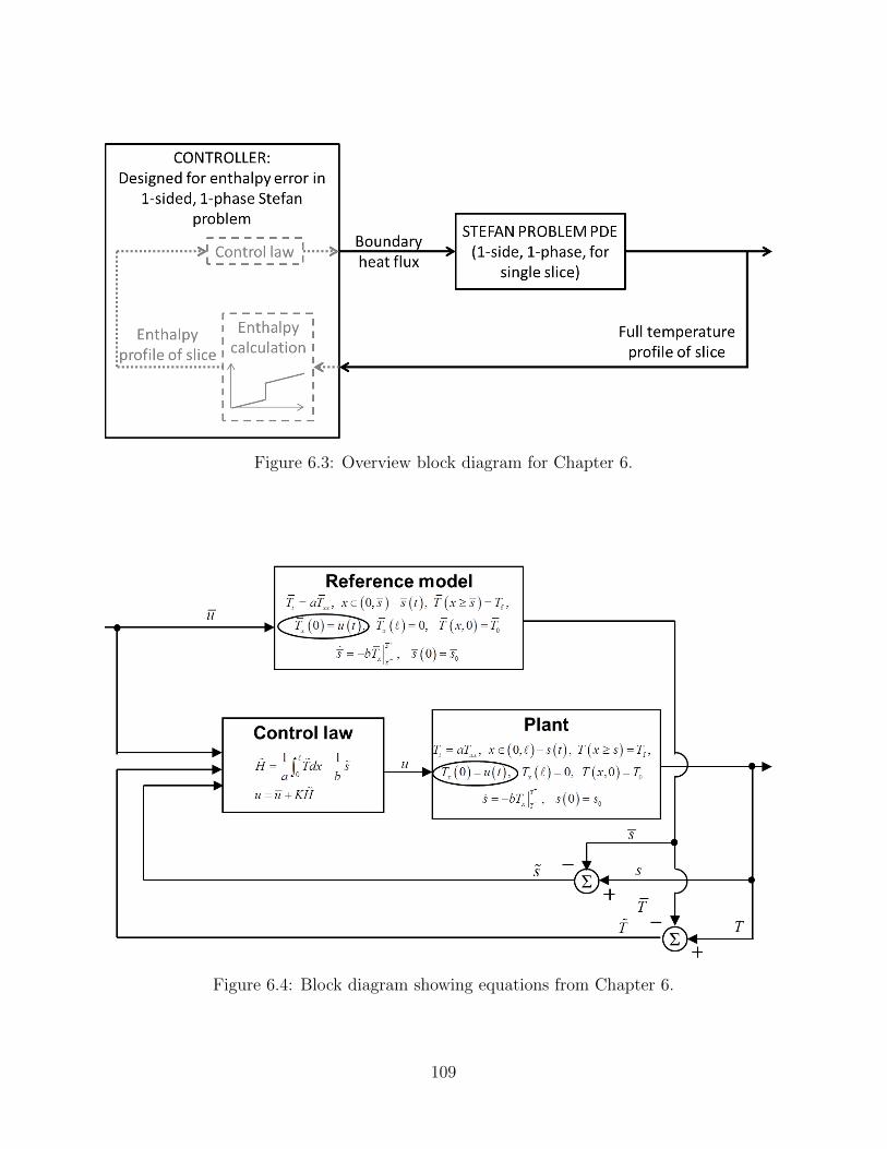
Figure 6.3: Overview block diagram for Chapter 6.


109

CHAPTER 7

EXTENSIONS FOR BETTER MODEL FIDELITY

7.1 The two–sided Stefan Problem

As mentioned in Chapter 1, the strand is bent from vertical to horizontal while in the caster.

This means that spray water will tend to pool on the top of the strand, but not the bot-

tom, leading to significantly different heat transfer, and therefore a symmetric temperature

distribution is not possible. Moreover, the inner and outer sides of the strand will undergo

tensile stresses at different points within the caster (times, in the 1D moving slice model),

so symmetric tensile distributions are not even necessarily desirable. Hence, the assumption

of symmetry should be dropped. The model (1.7)–(1.10) can be extended easily by includ-

ing both sides of the caster, giving two moving solid-liquid boundaries and two Neumann

boundary conditions.

Tt(x, t) = aTxx(x, t) , x ∈ (0, `)− s1 (t) , s2 (t) , (7.1)

T (s1(t) , t) = Tf = T (s2(t) , t) ,

Tx(0, t) = u1(t) , Tx(2`, t) = u2(t) ,(7.2)

T (x, 0) = T0(x) (7.3)

s1(t) = b(Tx(s−1 , t

)− Tx

(s+

1 , t)), s1(0) = s1,0

s2(t) = b(Tx(s−2 , t

)− Tx

(s+

2 , t)), s2(0) = s2,0.

(7.4)

Here, the material is liquid between s1 and s2, and solid otherwise. Assumption (A4) can

be adjusted to reflect this.

(A6) The initial conditions satisfy: 0 < s1,0 < s2,0 < 2`; T0 is piecewise smooth, continuous,

110

and non-decreasing; T0 (x) < Tf for all x ∈ (0, s1,0) ∪ (s2,0, 2`) and T0 (x) = Tf for all

x ∈ (s1,0, s2,0).

The reference profiles and errors can be defined equivalently.

7.1.1 Convergence proof

For the two-sided Stefan problem, Theorem 6.3.1 can be extended to the following:

Theorem 7.1.1. Denote

H2 :=

∫ 2`

0

h dx =1

a

∫ `

0

T dx+1

b(s1 − s2) . (7.5)

Let the reference and actual system both satisfy Assumptions (A6) and (A5), and the Neu-

mann boundary conditions satisfy

u1 (t) + u2 (t) = KH2 (t) , (7.6)

where gain K > 0. Then the reference temperature error T converges asymptotically to 0

uniformly over the domain, and both interface position errors converge to 0 asymptotically

as well.

Proof. The proof follows the same basic principle as the proof of Theorem 6.3.1. As in that

case, the Neumann boundary control can be shown to directly affect the total enthalpy error.

d

dtH = −u1 − u2. (7.7)

So, the control law (7.6) drives the enthalpy error to 0.

As in the previous chapters, temperature convergence is proven with a Lyapunov func-

111

tional. In this case,

V(T)

:=1

2

∫ `

0

T 2 dx

− a

bTf (s1 + s1)− a

bTf (s2 + s2)

+ 8a

bTf`

(7.8)

Taking the time derivative, using the PDE (7.1)-(7.4), and integrating by parts,

d

dtV(T)

= −aT (0) u1 + aT (2`) u2

− a∫ 2`

0

T 2x dx

− a

b

(T (s1) s1 + T (s1) ˙s1

)− a

b

(T (s2) s2 + T (s2) ˙s2

)(7.9)

To complete the proof requires the bounds on T and Tx that came from Poincare’s and

Agmon’s inequalities. These relied on knowing that T (`) = 0 due to symmetry, which is not

necessarily true any more.

There are two possible cases. First, the liquid phases of the reference and actual system

overlap at some point, i.e. T (xeq) = T (xeq) = Tf , for some 0 < xeq < 2`. Second, there

is no overlap. This necessarily means that s2 < s1, or s1 > s2. If the former is true,

Assumption (A6) means that T (s2) = Tf and T (s1) < Tf , while T (s2) < Tf and T (s1) = Tf ,

and the two temperature profiles are continuous. Therefore, they must intersect at some

point s2 < xeq < s1. Similar reasoning holds if s1 > s2. Thus, there must have a point

where the temperatures are equal, and T (xeq) = 0, which means Poincare’s and Agmon’s

inequalities can still be applied.

The remainder of the proof follows the same as for Theorem 6.3.1.

Unfortunately, as illustrated below, convergence under this proof is not necessarily guar-

anteed until after final solidification occurs.

112

7.1.2 Simulation results and discussion

In this section two algorithms for control of the two-sided Stefan problem are compared:

u1 = u2 =K

2

(1

a

∫ `

0

T dx+1

b(s1 − s2)

), (7.10)

and

u1 = K

(1

a

∫ `

0

T dx+1

bs1

)u2 = K

(1

a

∫ 2`

`

T dx− 1

bs2

).

(7.11)

Note that both (7.10) and (7.11) meet the criterion (7.6) for Theorem 7.1.1. However,

suppose the initial condition has an error as shown in Figure 7.1. Since the error in enthalpy

is symmetric, the control law (7.10) will not make any adjustment. The errors will eventually

converge, but not until after final solidification, as shown in Figure 7.2. For the intended

application of continuous casting, this puts the caster at risk of a whale.

Compare this with control law (7.11), which is simulated in Figure 7.3. The second control

law converges before final solidification. While these initial conditions are unrealistic, they

illustrate the importance of considering the convergence rate when using this control method.

7.2 Input saturation

An additional concern in actual casting applications is actuator saturation. The steel is

cooled by water sprays, and there are a strict upper and lower bounds on the spray rates.

The upper bound comes from the limits of the piping system, and the lower bound from the

minimum water flow rate necessary to produce a steady spray fan. Chapter 6 suggested that

this may be dealt with by decreasing the controller gain K. However, due to clogging, loss of

pressure, or other problems, the saturation bounds may even not be known. It is therefore

important to know whether the control law works if saturation is applied. So, denote input

113

Figure 7.1: Initial condition for simulations in Section 7.1.2.

114

Figure 7.2: Temperature error T for two-sided Stefan Problem (7.1)-(7.4), with initial con-ditions from Figure 7.1 and Neumann boundary control (7.10).

115

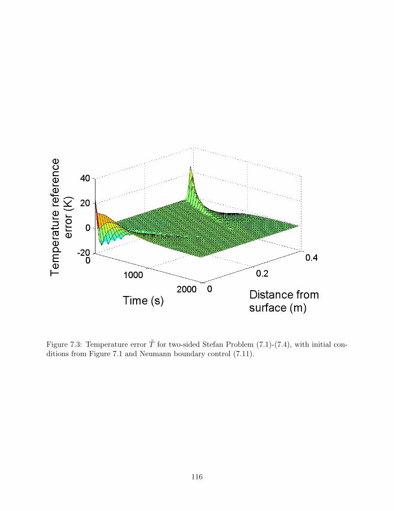
Figure 7.3: Temperature error T for two-sided Stefan Problem (7.1)-(7.4), with initial con-ditions from Figure 7.1 and Neumann boundary control (7.11).

116

saturation by

usat :=

uL, if u ≤ uL

u, if uL ≤ u ≤ uU

uU u ≥ uU

(7.12)

7.2.1 Convergence proof

It turns out that the enthalpy-based control algorithm will still converge, as long as some

control adjustment is possible around the reference profile. Specifically:

Theorem 7.2.1. Let u and usat be defined as in (1.8) and (7.12) respectively. Suppose there

exists ε > 0 such that

uL < u± ε < uU (7.13)

for all time, and T and s satisfy system (1.7)-(1.10) with boundary condition Tx (0, t) = usat,

then T converges uniformly to T and s converges to s.

Proof. In order to simplify notation, u will continue to denote the error between the desired

control effort and the reference control, and usat := usat − u will denote the difference under

actuator saturation. Using this notation, the derivative of H, calculated in (6.5), becomes

d

dtH = −usat (7.14)

If

−ε < u (t) = KH (t) < ε, (7.15)

at any time t, then (7.13) ensures uL ≤ u ≤ uU and saturation does not occur, i.e. u = usat.

In this case, (7.14) is the same as the calculation (6.5) in the proof to Theorem 6.3.1, so the

conditions for the proof still hold. Under those conditions, u from (6.6) is exponentially de-

creasing, and so (7.15) will continue to hold, the boundary control input will never saturate,

and convergence occurs as normal.

If saturation does occur, then either usat = uL− u or usat = uU − u. In either case, (7.13)

117

ensures that usat ≥ ε and furthermore

sign(usat) = sign(u) = sign(KH

)= sign

(H)

and also that |usat| ≥ ε Therefore, using (7.14),

d

dt

∣∣∣H∣∣∣ = sign(H) d

dtH = −sign(usat) usat = − |usat| ≤ −ε.

Therefore, the magnitude of H is strictly decreasing, and eventually (7.15) will be true,

which ensures convergence.

7.2.2 Simulation results and discussion

The condition (7.13) simply requires that there be some actual control adjustment available.

As long as there is any consistent room, however small, between the reference control and the

saturation bounds, the error will converge to 0. Under this assumption, the enthalpy error

will still move towards 0 until it is close enough that control law (6.6) does not saturate.

Figure 7.4 illustrates this convergence. The parameters used are still those given in Table 6.1,

and the initial conditions are still from Figure 6.1. The saturation bounds are uL = 2500

W/m · K and uU = 3500 W/m · K. As proven, despite saturation, the reference errors still

converge to 0.

An important extension of this result is to the case where the saturation bounds are

time-varying.

usat :=

uL(t) , if u ≤ uL(t)

u, if uL(t) ≤ u ≤ uU(t)

uU(t) u ≥ uU(t)

(7.16)

This should be considered because of the containment rolls mentioned in Chapter 1. While

the slice is under the containment rolls, the sprays cannot reach the surface. The sprays

have an indirect effect by drawing heat from the rolls, but the upper bound is very small.

However, the key to convergence is still to match the enthalpy. That is,

118

(a) Temperature error T with actuator saturation.

(b) Neumann boundary control with actuator saturation.

(c) Solidification front position s(t), comparing result with no control and (6.6) under saturation.

Figure 7.4: Illustration of Theorem 7.2.1 by numerical simulation of Stefan Problem (1.7)–(1.10), with initial conditions from Figure 6.1 and Neumann boundary control (6.6) undersaturation.

119

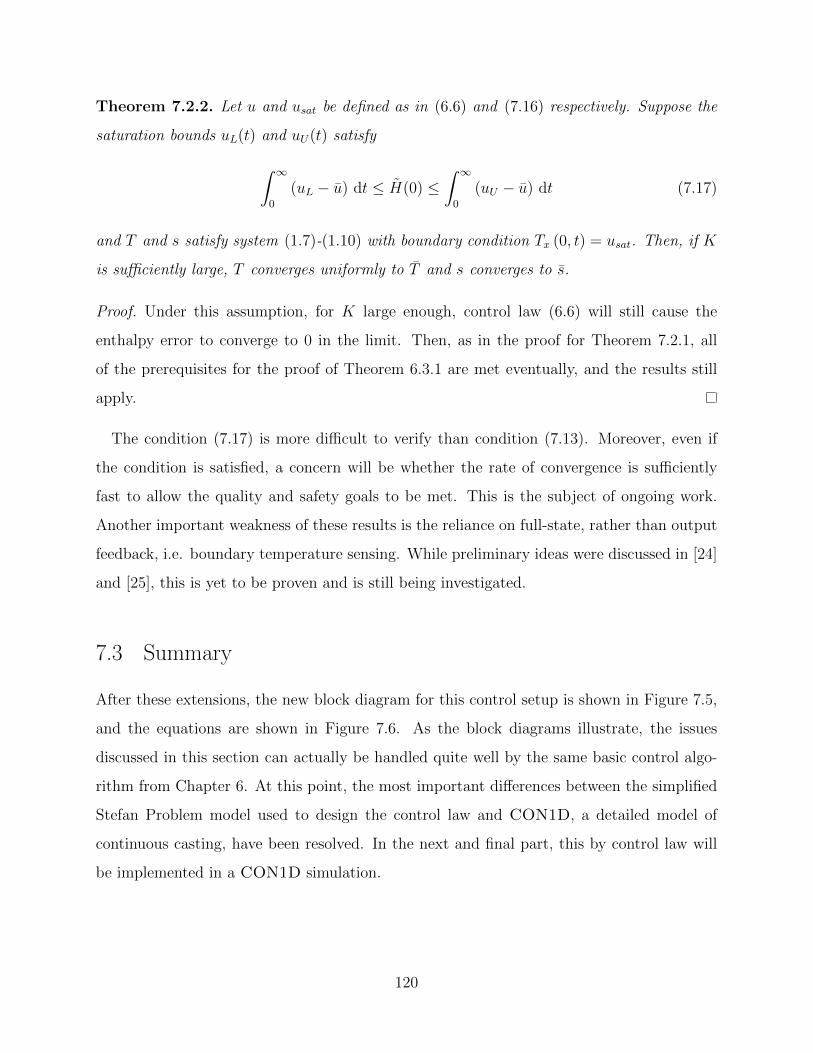
Theorem 7.2.2. Let u and usat be defined as in (6.6) and (7.16) respectively. Suppose the

saturation bounds uL(t) and uU(t) satisfy

∫ ∞0

(uL − u) dt ≤ H(0) ≤∫ ∞

0

(uU − u) dt (7.17)

and T and s satisfy system (1.7)-(1.10) with boundary condition Tx (0, t) = usat. Then, if K

is sufficiently large, T converges uniformly to T and s converges to s.

Proof. Under this assumption, for K large enough, control law (6.6) will still cause the

enthalpy error to converge to 0 in the limit. Then, as in the proof for Theorem 7.2.1, all

of the prerequisites for the proof of Theorem 6.3.1 are met eventually, and the results still

apply.

The condition (7.17) is more difficult to verify than condition (7.13). Moreover, even if

the condition is satisfied, a concern will be whether the rate of convergence is sufficiently

fast to allow the quality and safety goals to be met. This is the subject of ongoing work.

Another important weakness of these results is the reliance on full-state, rather than output

feedback, i.e. boundary temperature sensing. While preliminary ideas were discussed in [24]

and [25], this is yet to be proven and is still being investigated.

7.3 Summary

After these extensions, the new block diagram for this control setup is shown in Figure 7.5,

and the equations are shown in Figure 7.6. As the block diagrams illustrate, the issues

discussed in this section can actually be handled quite well by the same basic control algo-

rithm from Chapter 6. At this point, the most important differences between the simplified

Stefan Problem model used to design the control law and CON1D, a detailed model of

continuous casting, have been resolved. In the next and final part, this by control law will

be implemented in a CON1D simulation.

120

Figure 7.5: Control block diagram for Chapter 7.


121

Part III

Synthesis and future work

122

CHAPTER 8

LOOP CLOSURE ISSUES AND UNCERTAINTYANALYSIS

In the first part of this dissertation, I described a real-time model that is, in control ter-

minology, an open-loop estimator/predictor of the temperature and solidification in a steel

caster. Through rigorous validation to past plant trials, and integration of measurements of

numerous casting conditions during operation, that computational model achieves excellent

accuracy. The information

In the second part, I considered a greatly simplified model that allowed me to develop a

working control law for the distributed temperature profile. In this chapter, I will link the

two approaches together to move towards a practical control solution for continuous steel

casting.

8.1 Applicability of assumptions to steel casting

In Part II, the Stefan problem was used as a model of the continuous caster to design a control

law. The control law (7.11) was proven to work for the two-sided Stefan problem, even under

actuator saturation. However, saturation is not the only problem with the actuation in a

caster. Figure 2.6 in Chapter 2 shows the actual boundary conditions in the caster, in terms

of convection heat transfer coefficients. The applicable limit on the boundary condition is

(7.16) which was proven to converge under the condition (7.17). I have not been able to

verify this directly, but I will nonetheless attempt to control the temperature of a slice of

the continuous caster using only water sprays in simulation.

One important detail this creates is that control law (6.6) required direct control of the

heat flux at the surface. However, heat flux from the water sprays follows the nonlinear

convection heat transfer coefficient of Nozaki, in Equation (2.10). Combining these two

123

equations, the change in spray water flow rate, Qspray that will satisfy equation (6.6)

Qspray :=

(u+KH

A (1− bTamb) (T − Tamb)

) 1c

(8.1)

where A, b, and c are the parameters of the Nozaki model as in Section 2.4.1.

The control law also requires feedback of the entire distributed temperature profile of the

slice, which is clearly not available. Even if the surface temperature could be measured, which

cannot be reliably done, the internal temperature is impossible to measure. The obvious

approach here is to borrow the idea of Part I and use an open-loop, but comprehensive and

well-calibrated computational model as a replacement for physical sensors. For the slice, this

would be CON1D. Although CON1D is based on the effective specific heat PDE, (1.6),

the enthalpy can still be calculated as the inverse of (1.5)

h(T ) =

∫ T

0

c∗p(τ) dτ. (8.2)

In practice, since the control law will end up subtracting enthalpies, the integral can start

at a higher reference temperature to speed up the calculation.

Incorporating these two changes, the proposed control algorithm is shown as a block

diagram in Figure 8.1. The control algorithm gets an estimate of the slice temperature from

CON1D calculates the enthalpy by (8.2) (a static nonlinear function), computes the control

law (7.11) for the two-sided Stefan Problem, and then uses equation (8.1) (a second static

nonlinear function) to get the requested water flow rates. These are sent to the caster, and

may be changed due to saturation or physical behavior of the piping system. As discussed

in Chapter 7, neither effect should prevent convergence.

Figure 8.2a shows a simulation of the Nucor Decatur caster under normal casting condi-

tions for a low carbon steel. Note the characteristic jumps in temperature at the surface,

where the steel moves between rolls and sprays. Figure 8.2b shows what happens to the

temperature relative to this nominal result when the superheat increases by 10C, e.g. from

an incoming ladle of new steel, and the mold heat flux decreases by 25%, e.g. due to a

change in the gap from mold powder solidifying or sticking, but no adjustment is made to

124

Figure 8.1: Control block diagram for Section 8.1.

the water spray rates. The steel exits the mold approximately 14 s into the simulation,

where the temperature error reaches the peaks. After this point, as in the uncontrolled sim-

ulations of the Stefan problem in previous chapters, the temperature approaches a non-zero

steady-state error, but only after the shell is fully solid, and indeed after the slice has left

the caster, around 200 s into the simulation.

Now, Figure 8.2c shows what happens when the water is adjusted according to (8.1). In

this case, the temperature returns to its nominal value over time. The trade-off, of course, is

that the surface temperature is lower than desired in the early zones, while the control law

seeks to cancel out the difference in enthalpy. Figure 8.2d shows that the “shell thickness”

is converging as well. Since this is an alloy, there is a mushy zone in the steel, so the

shell thickness is not well-defined. As discussed in Section 3.1.2, a solid fraction of 0.7 is

commonly given as sufficient to contain the liquid core, so that is used to define the shell

thickness in Figure 8.2d. Without control, the metallurgical length is longer, which could

lead to a whale. With this control law, however, the metallurgical length is the same as its

original length.

125

(a) Temperature at Nucor Decatur casterunder nominal casting conditions.

(b) Temperature error when conditions inmold change, and water flow rates are notadjusted.

(c) Temperature error when conditions inmold change, and water flow rates are ad-justed according to (8.1).

(d) Shell thicknesses for the nominal, un-controlled, and controlled cases.

Figure 8.2: Application of enthalpy-based control algorithm to computational model ofNucor Decatur steel caster.

126

8.2 Quantitative uncertainty analysis of the estimator

This work assumes that a computational model was used as the basis of full-state feedback in

certainty equivalence. I claimed earlier, without giving reason, that the computational model

would be more trustworthy than in-plant measurements. In this chapter, I will attempt to

quantitatively estimate the uncertainty in the model.

There are, roughly speaking, three sources of error in the model: error in the numerical

method, error in the calibration of certain parameters in the model to the actual caster, and

error in the measurements of casting conditions used as inputs to the model. I will deal with

each of these separately.

8.2.1 Numerical error: grid convergence study

The numerical model CON1D employs a finite-difference scheme that is “second-order ac-

curate” in space step size and “first-order accurate” in time step size. That is, the error

should be O(∆x2,∆tFD). In practice, this only holds true until the grid spacing becomes

small enough that floating point error begins to dominate the finite-difference error, as will

be shown shortly. Hence, I will assume that the finite difference error is approximately

∆TFDM ≈ C∆tFD∆tFD + C∆x∆x2. (8.3)

To put numbers to the constants C∆tFDand C∆x, I performed a grid convergence study,

changing the finite difference grid size and comparing the results. I ran CON1D repeatedly

under the nominal casting conditions used in the previous section, based on the Nucor De-

catur thin-slab casting at their most common casting speed of 3.5 m/min. Then, I averaged

the difference between the predicted temperatures and a baseline case. The choice of base-

line is arbitrary, but the trend of the differences is meaningful. These results are shown in

Figure 8.3.

As seen in Figure 8.3a, the temperature tends changes linearly with decreasing finite

difference time step ∆t, as expected for this method. The baseline case here is ∆tFD = 0.03 s

and ∆x = 0.99 mm. The last two points show the error increasing again due to floating

127

(a) Temperature versus finite difference stepsize ∆tFD, with ∆x = 0.99 mm showing bestlinear fit.

(b) Temperature versus finite difference stepsize ∆x, with ∆tFD = 0.005 s showing bestquadratic fit.

Figure 8.3: Grid convergence study of finite difference parameters in CON1D.

point error. The least-squares linear fit to these errors is

difference = −3.35− 98.2∆tFD,

and the resulting value of R2 is 0.936, indicating a very good fit.

In Figure 8.3b, the temperature changes with the square of the finite difference space step

∆x2, again as expected. The baseline case here is different from the previous figure. For

this figure, ∆tFD = 0.005 s and ∆x = 1.98 mm for the baseline. The reason for the smaller

time step is because the explicit finite difference method is numerically unstable when

α∆tFD

∆x2>

1

2

Hence, reducing the space step can make the numerical method unstable, but stability can

be gained by reducing the time step. The time step for Figure 8.3b was chosen small enough

that all cases were numerically stable without changing the time step, ∆tFD. In this case,

the least-squares quadratic fit is

difference = 4.07− 0.929∆x2,

128

with an R2 of 0.956. Again, this is a very strong fit.

However, two features of Figure 8.3b deserve special discussion. First, the error does not

appear to ever increase due to floating point error. Any smaller space step would require

reducing the time step further to maintain numerical stability. As seen in Figure 8.3b,

decreasing the ∆t below 0.005 s could lead to floating point errors from the small time

step. Hence, no further cases with smaller time step can be performed with these material

properties. Second, the temperature increases as ∆x decreases, whereas it decreased as ∆tFD

decreased. The error for this FDM is only known to be O(∆x2,∆tFD). This implies nothing

about the sign of the error. Hence, I will consider the least squares coefficients to be bounds

on the absolute error due to the finite difference approximation, and discard the signs. That

is,

∆TFDM ≈ ±98.2∆tFD ± 0.929∆x2. (8.4)

8.2.2 Calibration error: comparison with measured values

The primary source of calibration error is in the boundary conditions. In the mold, the

boundary heat flux qmold is set according to the simplified model discussed earlier. Figure 2.5

shows this prediction relative to more accurate predictions from more detailed models. The

maximum error in heat flux relative to the more accurate values is 30.2 %. However, the

error appears to be consistently positive higher in the mold, and negative lower in the mold.

Since the average is matched, it would over estimate the uncertainty in the temperatures.

Instead, the error is simply assumed to be linear in distance from the meniscus, z. Assuming

the error is linear with z, this would mean that

∆qmold ≈ 0.302z − 1

2zm

12zm

qmold (8.5)

In the spray region, the boundary heat flux from water sprays is modelled with Nozaki’s

relationship, with parameters A, b, and c. The heat flux for the rolls is chosen relative to

the Nozaki heat transfer coefficient, along with parameter froll. The uncertainty in these

parameters is more difficult to determine, as there are not as many reliable measurements to

129

compare to in the spray zones. As discussed in Chapter 3, the primary measurement these

coefficients were calibrated to match was the observed ML during the caster trial at Nucor

Decatur. This trial was able to determine the ML to be approximately at one of the drive

rolls. This means any error these parameters induce in the prediction of ML should be less

than one roll pitch in either direction, i.e. 207 mm. Consensor’s resolution for ML is only

10 mm, so I will round this to 210 mm. Another complication is that during the trial, the

casting speed could only be changed in increments of 5 in/min (0.127 m/min). The casting

speed that led to the roll turning in the trial cannot be known with any more precision then

that. Thus, a reasonable upper bound for the uncertainty in these parameters is whatever

change causes the metallurgical length to increase or decrease at least 210 mm when the

casting speed is decreased or increased, respectively, by 0.127 m/min.

Looking at equations (2.10) and (2.12), it is clear that increasing A, c, and froll will increase

the heat transfer coefficients in the spray zone, and increasing b will decrease the heat transfer

coefficients. Thus, increasing the first three will decrease the predicted temperature, and

increasing the latter will increase the temperature. Unfortunately, the ML measurement

only truly allows comparison with the overall heat flux, and not the effect of each individual

parameter. Hence, I will assume that each parameter is off by the same percentage relative

to its calibrated value. Since b has the opposite effect of the other three, I will assume it

changes in the opposite direction of the other parameters. I will also assume that these

parameters are off by the same percentage in every spray zone.

Figure 8.4 shows the results of a simple iterative search on these parameters. As shown

in the figure, increasing or decreasing the parameters by at most 6.5% relative to their

calibrated values changes the predicted ML by 210 mm for the given uncertainty in speed.

Hence, this is considered to be the calibration error in these parameters. This is, as discussed

above, only a rough estimate, as there are many ways to vary parameters that would result

in greater differences but the same predicted ML. For example, increasing A but decreasing

froll could leave the ML the same, or changing parameters differently in different parts of

the caster.

This gives reasonable assumptions of uncertainty in the boundary heat fluxes in the mold

and spray regions of the caster, summarized in Table 8.1. However, these are only the

130

Figure 8.4: Effect of changing spray zone heat flux parameters on shell thickness.

131

Table 8.1: Assumed uncertainties in calibration of computational model / estimator ofthin-slab caster.

Description Variable Nominal ±Uncertainty Units Effect on surf. temp.Mold heat flux ∆qmold 2.366 Eq. (8.5) MW/m2 decreases

Spray param. A A 0.3925 0.1052 decreasesSpray param. b b 0.0075 0.0005 increasesSpray param. c c 0.55 0.037 decreases

Roll fraction froll 0.29 0.0195* decreases*Averaged over all spray zones.

boundary conditions, and the real uncertainty of interest is the strand temperature. This

will be addressed in the next subsection.

8.2.3 Input error: parametric study

The final source of error is error in the measurements from the caster that are input to the

model when it is run. There are a wide variety of these, and they are specified in table

8.2, with nominal values under usual casting conditions at Nucor Decatur, and assumed

uncertainty in the measurement. Wherever possible, these are based on actual data collected

from the steel mill. In her work on mold heat removal, Duvvuri [48] collected and processed

two years of casting conditions from the Nucor Decatur plant database included maximum

and minimum values over a ten minute interval. Those ranges were used for the uncertainties

where available. For measurements for which this data is not available, measurement error

is estimated from experience with casters.

The analytical method that modelers use to examine the effect of all of these on the output

temperature is to find the derivatives of temperature with respect to each input, and get a

first-order approximation of the output uncertainty in this manner. While this is currently

being performed for this model, results are not yet available. Instead, for the purposes of

this work, I have used a simple parameteric study to estimate the uncertainty.

Increasing any given measurement, at least in a neighborhood of the nominal conditions,

either increases or decreases the surface temperature. For some of the measurements, e.g.

pour temperature, the effect is obvious and needs no explanation. For others, the effect

132

Table 8.2: Assumed uncertainties in measurements input to computational model / esti-mator of thin-slab caster.

Description Variable Nominal ±Uncertainty Units Surf. temp. changeCasting speed vc 3.5 0.03 m/min increases

Pour temp. Tpour 1550 5 C increasesMold heat flux qmold 2.366 0.05 MW/m2 decreasesCarbon content pC 0.05 0.002 weight-% increases**

Spray water Qspray 93.5* 1* L/min/row decreasesSpray width Wspray 1.37* 0.01* m increasesSpray length Lspray 0.05* 0.01* m increasesRoll contact θroll 10 5 increases**

Ambient temp. Tamb 25 10 C increases**

*Averaged over all spray zones.**Average effect on surface temperature determined by simulation near these nominal conditions,and may not hold for all conditions.

is less certain. For example, increasing the length that the spray impinges on the steel

surface increases the area where heat is removed, but decreases the local water flux. These

simultaneous changes have opposite effects on temperature, and it is not clear which, if any,

dominates. As indicated in the table, in this case, CON1D was run to determine the effect,

and the temperature was higher on average for higher spray lengths. It is important to note

that the effect of these inputs is nonlinear and related to many other parameters, so this

may not hold for all spray lengths.

Once the effect of each individual parameter was determined, an approximate upper and

lower uncertainty bound for the temperature could be determined by choosing the parameters

to maximize or minimize, respectively, the temperature. The results are shown in Figure 8.5.

8.3 Use of sparse measurements for re-calibration

Figure 8.6 shows the information used and produced by the software sensor Consensor,

as described in Chapter 2. As the block diagram illustrates, the method is open-loop in

nature. The only measurements available are not affected by the output to be controlled,

temperature of the strand. As discussed in Section 3.1.1, pyrometers in the spray zone

are not reliable, and the computational model is actually assumed to have more accuracy.

133

(a) Uncertainty in the temperature predic-tion of CON1D.

(b) Uncertainty in the shell thickness predic-tion of CON1D.

Figure 8.5: Results of uncertainty quantification in CON1D, including uncertainty in nu-merical method, calibration, and measurements.

However, Figure 8.5 clearly shows that there is significant uncertainty in the computational

model as well. The estimation problem will be discussed in the next chapter. In this Section,

instead of estimation, the problem of automated re-calibration will be considered. This still

relies on a perfectly accurate temperature measurement, but only at one point in the caster.

Looking at the problem another way, this is a common problem in modelling: adjust

parameters in a computational model to match sparse measurements, as described in Sec-

tion 3.1. In general, this calibration problem assumes that the system dynamics are known

except for a finite set of unknown parameters. In this case, the least-well-known of these

parameters are all related to the boundary heat flux. Although the Stefan problem is non-

linear, it is still parabolic in most of the strand, which allows some hope of re-calibrating

the model in real-time.

Lemma 8.3.1. Let T1(x, t), s1(t), and T2(x, t), s2(t), be solutions to the 1-D Stefan problem

(1.7)–(1.10) with the same initial condition, T1(x, 0) = T2(x, 0), s1(0) = s2(0), that satisfies

the single-phase Stefan problem assumption (A4), and the same material properties a and

b. Then, if the boundary heat fluxes satisfy u1(t) ≥ u2(t) ≥ 0∀t, the temperatures satisfy

T1(x, t) ≤ T2(x, t).

Proof. The proof is a straight forward application of the maximum principle for parabolic

PDEs. Even though the Stefan problem itself is nonlinear, for given boundary positions s1

134

Figure 8.6: Block diagram of measurements and predictions in software sensor Consensor.

135

and s2, the PDEs are uniformly parabolic on the open spatial domain (0, `) − s1, s2. In

particular, the maximum principle for parabolic PDEs applies [29], i.e. that the maximum

and minimum values of the functions or its spatial derivatives at any given time occur either

at the boundaries or initial conditions.

Moreover, since∂

∂t(T1 − T2) = a

∂2

∂x2(T1 − T2) ,

so the maximum principle applies to T1 − T2 as well. By assumption,

u1(t) =∂T1

∂x(0, t) ≥ u2(t) =

∂T2

∂x(0, t) ,

and∂T1

∂x(`, t) =

∂T2

∂x(`, t) = 0.

From the maximum principle, this means that

∂T1

∂x≥ ∂T2

∂x∀x, t. (8.6)

Then, comparing the above relationship with the boundary velocity (1.10), s1 ≥ s2 for any

time t, and since the initial conditions are identical, s1 ≥ s2 also.

On the interval (s1, `), trivially T1(x, t) = Tf = T2(x, t), and on the interval (s2, s1), equally

trivially, T1(x, t) ≤ Tf = T2(x, t). Thus, it is only necessary to consider the interval (0, s2).

Under the boundary conditions (1.8) for the Stefan problem, T2(s2, t) = Tf ≥ T1(s2, t).

Then, for any x in this subinterval,

T1(x, t) = T1(s2, t)−∫ s2

x

∂T1

∂xdx ≤ T2(s2, t)−

∫ s2

x

∂T2

∂xdx = T2(x, t) ,

where the inequality follows from (8.6).

An immediate consequence of this Lemma is that certain simple calibration problems

must have a unique solution. For example, if the heat flux follows the models discussed

in 2.4.1 excepting only that the spray parameter A is unknown. From (2.10), increasing A

136

increases the boundary heat flux. Then, by the lemma, if the pour temperature Tpour and a

measurement of the temperature at any single point in the caster, T (xmeasure, t), are known,

the actual value of A can be exactly determined. More precisely,

Theorem 8.3.1. Let T (x, t) be the solution to the single-phase Stefan problem (Equations

(1.7)–(1.10) with initial condition satisfying assumption (A4)) with boundary condition (2.9),

where one parameter is unknown, but the initial condition T (x, 0) and one single other

point and time, T (xmeasure, tmeasure) are known. If the boundary heat flux has a monotonic

dependence on the parameter, then the parameter can be found exactly.

Proof. Given Lemma 8.3.1, and the monotonic dependence on heat flux, there is only one

parameter that will match the measurement from the initial condition. Furthermore, the

monotonicity means that the parameter can be found by, for example, a simple search

algorithm.

Obviously this is a very weak conclusion. Many of the model parameters, in particular A,

b, c, and froll do have a monotonic dependence on heat flux locally. However, they may vary

through the caster, so the assumption of a single missing parameter is not very likely. Still,

this the most that I can say at present.

Figure 8.7 shows a simulation of this. In the simulated case shown in the figure, the

parameter A is equal to 2 for the actual system and 1.57 for the estimate. At 6 m from the

meniscus, the surface temperature of the steel is collected, for example from a pyrometer,

dragging thermocouple, or infrared camera. Then, the estimate adjusts the parameter A

using the basic Newton search method. The algorithm reduces the temperature error to less

than 1% in two iterations, which can be easily performed in time to continue the simulation

on an actual caster. The calculated A is 1.99. This was then used for the remainder of the

simulation.

Figure 8.8 shows the adjusted information flow used in these simulations. Compared

to Figure 8.6, this proposed estimator is no longer completely open-loop, and is able to

temporarily close the loop when pyrometer measurements are received. Figure 8.1 shows a

block diagram for this final suggested control system of this Chapter. The dash-dot lines

for the surface temperature measurement are meant to indicate that re-calibration can only

137

(a) Inner radius surface temperature. (b) Inner radius shell thickness.

Figure 8.7: Simulation of CON1D showing mid-simulation re-calibration to match surfacetemperature measurement 6 m from meniscus.

occur only when whatever few temperature sensors are available give a measurement. As

more temperature measurements become available, this re-calibration can occur more often.

There may even eventually be enough measurements to allow true output-feedback, which is

discussed in the next chapter. The other weakness of this proposed control system is that it

is limited to a single slice of the caster, rather than the entire strand. This is also discussed

in the next chapter.

138

Figure 8.8: Block diagram of measurements and predictions in proposed slice software sensorwith sparse re-calibration.

139

Figure 8.9: Control block diagram for Section 8.3.

140

CHAPTER 9

CONJECTURES, SUGGESTIONS FOR FUTUREWORK, AND CONCLUSIONS

As has been discussed throughout the preceding chapters, the simulations have tended to

produce better results than can currently be proven. In this chapter, the simulation evidence

supporting various extensions of the existing work is collected, and conjectures are given

regarding possible future areas of investigation.

9.1 Conjectures

9.1.1 Exponential convergence

The typical linear heat equation, under a similar control law to the ones presented in this pa-

per, can be shown to have exponential convergence [54]. The simulations shown (Figures 6.2,

8.2, and even the output feedback in 9.3) appear to be showing exponential convergence of

the temperature and solidification front. Unfortunately, I was unable to prove this.

Figure 9.1 shows repeated simulations of the Stefan problem (1.7)–(1.10) with the full-

state-feedback control law (6.6), and a wide range of initial conditions, collected in Fig-

ure 9.1a. As Figure 9.1b shows, there appears to be an exponential bound on the L1 norm

of the enthalpy error, i.e.

∥∥∥h(x)∥∥∥

1=

∫ `

0

∣∣h(T (x))− h(T (x)

)∣∣ dx. (9.1)

Although all simulations appear to be bounded by this exponential convergence rate, I cannot

prove that it holds.

141

(a) Initial conditions of simulations, andnominal initial condition.

(b) Normalized L1 error of enthalpy fromsimulations, and estimated rate of exponen-tial convergence.

Figure 9.1: Simulations investigating exponential convergence for Stefan problem (1.7)–(1.10) with control law (6.6).

9.1.2 Output-injection observer

Work in the industry continues on installing reliable pyrometers in the spray zone, but an

actual product is likely years away from completion. Once such a product is available, the

sparse recalibration method discussed in the previous section could be replaced by actual

estimation. Even with such sensors, only the surface temperature could realistically be

measured. So, the problem to resolve in this hypothetical future is to find a control law that

works with boundary (Dirichlet) sensing. The obvious approach is to design an estimator

and use certainty equivalence.

Returning to the calculation (6.10), if

u (0) T (0) ≥ 0 (9.2)

then the estimate (6.3) still holds, and the invariance principle can be applied. However, the

total enthalpy may not converge to 0, so temperature convergence does not imply convergence

of the interface position. In fact, for an arbitrarily small temperature error, the interface

position error can still be arbitrarily large. To summarize:

Theorem 9.1.1. Suppose the reference system and actual system satisfy assumptions (A4)-

142

(A6) and condition (9.2). Then the reference temperature error converges uniformly to 0.

In [24], a similar result was proposed as the basis for an estimator: set an estimate(T , s

)of the actual system that is a solution to (1.7)-(1.10) with left-hand boundary condition

T (0, t) = T (0, t) .

Under Theorem 9.1.1, the temperature estimation error should converge to 0, but the inter-

face position estimation may not converge to the true location. Moreover, in simulation, this

estimate converges only slowly. Still, this is one possible approach to an output-feedback

control law.

In simulations, better performance has been achieved using an estimation procedure that

adjusts the solidification front position as a function of the surface temperature estimation

error. The method, which is not yet proven to work, is as follows:

Let T and s be an estimate of the temperature T and interface location s, respectively.

Let the estimates satisfy the following PDE:

Tt (x, t) = aTxx (x, t) , x ∈ (0, `)− s (t) , (9.3)

T (s (t) , t) = Tf , Tx (0, t) = u (t) , Tx (`, t) = 0 (9.4)

T (x, 0) = T0 (x) , (9.5)

˙s (t) = −b(Tx(s(t)+)− Tx (s(t)−))+ L

(T (0, t)− T (0, t)

), s (0) = s0 (9.6)

where the initial conditions satisfy Assumption (A4) and the estimation gain L > 0.

Conjecture 9.1.1. Suppose (T, s),(T , s

), and

(T , s

)all satisfy the conditions for Theorem

6.3.1. Then under the control law

u = u−K[

1

a

∫ `

0

(T − T

)dx− 1

b(s− s)

], (9.7)

the temperature reference and estimation errors uniformly converge to 0, and the interface

position reference and estimation errors converge to 0.

143

Figure 9.2: Block diagram showing equations from Section 9.1.2.

A block diagram showing the structure of the equations is given in Figure 9.2. Figure 9.3

shows a simulation using this output-feedback control law. The initial estimation is the same

as the reference, i.e. T0 = T0 The estimation and reference errors appear to be converging

to 0 exponentially. However, this apparent result remains conjecture, and is a subject of

ongoing work. The key problem in applying the ideas of the previous chapters lies in showing

the enthalpy of the estimator, system, and reference all converge. In theory, the output

estimation error T (0)−T (0) can be zero while the solidification front estimation error s− s,

and consequently the enthalpy estimation error, is arbitrarily small. In simulations, this

output injection avoids such cases, but I cannot prove it.

144

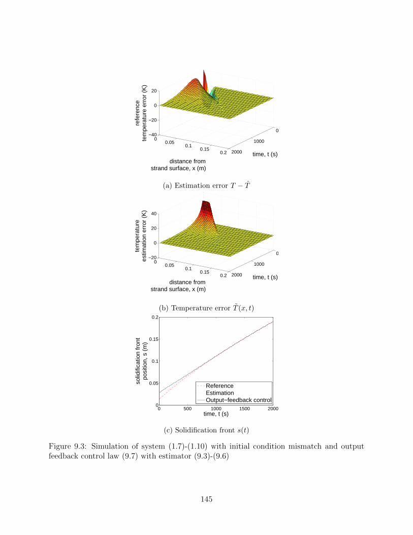
0

1000

2000

00.05

0.10.15

0.2

−40

−20

0

20



refe

renc

ete

mpe

ratu

re e

rror

(K

)

(a) Estimation error T − T

0

1000

2000

00.05

0.10.15

0.2

−20

0

20

40



tem

pera

ture

estim

atio

n er

ror

(K)

(b) Temperature error T (x, t)

0 500 1000 1500 20000

0.05

0.1

0.15

0.2

time, t (s)

solid

ifica

tion

fron

tpo

sitio

n, s

(m

)

ReferenceEstimationOutput−feedback control

(c) Solidification front s(t)

Figure 9.3: Simulation of system (1.7)-(1.10) with initial condition mismatch and outputfeedback control law (9.7) with estimator (9.3)-(9.6)

145

9.2 Future work

The issues this thesis attempts to deal with have not been definitively solved. There are

problems, both in the application of these results and the development of new control theory,

that I believe are waiting to be solved.

9.2.1 Proving conjectures

Obviously, the clear next objective in this work is to prove the conjectures of the previous

section. I think the approach most likely to work is to follow the method used in Part II:

finding a Lyapunov functional and using estimates and inequalities to prove the desired

result. For exponential convergence, based on Figure 9.1, the clear choice of a Lyapunov

functional is the L1 norm of the enthalpy. I have tried studying this, and was unable to prove

exponential convergence for it. It is very possible that there is something that I have missed.

Of course, it is also possible that Figure 9.1 is misleading, and the exponential convergence

shown does not hold for all initial or boundary conditions. For output feedback, I do not

see an obvious Lyapunov functional. I have not yet been able to prove even convergence of

the estimator, much less convergence of the output-feedback control law. Again, it is likely

that I am looking at the wrong Lyapunov functional, or am missing a key estimate.

Finally, the use of this control law for allows, in Chapter 8, is not yet proven either, despite

it performing well in simulation. This is more difficult to resolve with the current approach,

because the “mushy” zone of the alloy means the problem cannot be neatly divided into

subdomains on which the error follows a linear parabolic PDE. Another possible approach

to this, and the other conjectures, is to abandon the Lyapunov stability theory and examine

the solutions of the error system using more sophisticated functional analysis.

9.2.2 Analysis of the non-linear operator

As mentioned in Chapter 1, mathematicians (see [57], which references [28]) have been

able to prove that the Stefan problem PDE generates a nonlinear semigroup in the Banach

space of L1 functions on the spatial domain. This semigroup defines “generalized” solutions,

146

meaning not necessarily differentiable in time, to the Stefan problem. It may be possible

to prove differentiability under some assumptions to regularize the system. Moreover, the

semigroup can be shown to be bounded in the operator norm, making the system stable in

the Lyapunov sense. These results can be also easily extended to the general enthalpy PDE

1.2.

It would seem possible that further examination of these operators could prove the desired

convergence, and at the same time extend the results to alloys. However, this is certainly

not trivial. In particular, two problems need to be resolved. First, exponential, rather

than simple stability must be proven. For the semigroup, this requires conditions on the

spectrum of the operator. Second, the error system is actually time-varying. The paper [28]

does discuss conditions under which time-dependent operators generate semigroups, which

may be possible to apply to the enthalpy PDE reference error system.

9.2.3 Spray-zone control

The most critical step standing between the current algorithm and implementation is that

the current control only follows a single slice of the caster. At any point in the caster, the

work in this dissertation implicit assumed that the water flow rate can be chosen to best suit

that particular slice’s temperature. Casters, however, only have a handful of spray zones

in which the water flow rate through every nozzle is the same. Any slice in each zone will

receive the same water flow rate. Rather than following material as it moves through the

caster, which was useful for simplifying the governing nonlinear PDE to a 1-D problem that

could be easily analyzed mathematically, the spray zone covers a fixed 2-D spatial domain.

There are two problems with designing a similar enthalpy-based control law.

First, the temperature upstream of the spray zone cannot be controlled by changing the

water in the spray zone. Second, by studying a fixed spatial domain, advection must be

considered at the same time as conduction. This shows up as a term vc∂T∂z

in the PDE. That

is, changing casting speed actually changes the differential operator. Both problems lead

to the same conclusion: matching a fixed reference profile in a spray zone is fundamentally

impossible.

147

That being said, this does not mean control of the spray zone is impossible. The real

process goals discussed in Chapter 1 only require controlling certain parts of the spray

zone, for example controlling the surface temperature to prevent transverse cracks and the

temperature at the end of the zone to prevent whales. Hence, I believe the best option for

applying this approach to the actual caster is to develop a reference profile generator. The

goal of such a program is to develop a good, in terms of safety, production, and quality,

reference profile in response to changing casting speed and upstream conditions. Then a

similar control law to the ones presented here could regulate the temperature to match the

desired reference.

9.3 Conclusions

The main conclusion I would offer future researchers on this problem is to work with the

system dynamics (as in Chapter 6), not against them (as in Chapter 5). In effect, the idea

behind the control law of Chapter 6 is to match the internal energy, and then let diffusion

take over to get the temperature to match. Despite the simplicity, this method even works

on the more complicated model in Chapter 8.

In retrospect, it also suggests an explanation for why the PI controllers of Chapter 2 is

able to handle the system so well in Chapter 4. Although the system nonlinearity is difficult

to analyze mathematically, in function it acts as linear heat diffusion with a nonlinear state-

dependent heat sink that luckily only changes slowly. Thus, the surface temperature acts as

a linear first-order system with a constant disturbance.

148

APPENDIX A

NUMERICAL SIMULATION BACKGROUND

The simulation technique used in Part II and Chapter 9 is a straightforward calculation of

(1.2) using the Finite Difference Method (FDM). Denote the discretized temperature as

T i (t)

ni=0

:= T (i∆x, t)ni=0 (A.1)

where

∆x :=`

n(A.2)

is the grid spacing. Then, the well-known second–order accurate difference approximation

for the second spatial derivative is

d

dth(T i)

= kTxx (i∆x, t) = k

(T i+1 − 2T i + T i−1

(∆x)2 +O((∆x)2)) . (A.3)

Therefore, using the simple forward Euler integration scheme in time for the PDE (1.2),

h(T i (t+ ∆tFD)

)≈ h

(T i (t)

)+ k

T i+1 − 2T i + T i−1

(∆x)2 ∆tFD. (A.4)

Obviously, this only applies to the internal nodes, for which T i−1 and T i+1 are within

the problem domain. For this to be applied to the boundary nodes i = 0 and i = n would

require values for T−1 and T n+1, respectively, which are not physically meaningful in the

discretization scheme given, since they refer to points outside the problem domain.

However, the boundary conditions (1.3) should apply, and this suggests a way of creating

these “dummy node” values. If T−1 did exist, then applying the boundary condition and

the second–order accurate difference equation would mean that

149

Tx(0, t) =T 1 − T−1

2∆x+O

((∆x)2) = u. (A.5)

Solving this for the dummy node T−1, and gives the approximation

T−1 ≈ T1 − 2u∆x. (A.6)

This approximation can be used in (A.4) to update the boundary node i = 0. Similarly,

the approximation for node i = n uses the dummy node

Tn1 ≈ Tn−1, (A.7)

based on the boundary conditions.

Altogether, the following procedure is used to numerically integrate the PDE using this

FDM.

1. From the previous nodal temperature values, calculate the new nodal values of the

enthalpy h(Ti) using equations (A.4)–(A.7).

2. From these new enthalpy values, calculate the new nodal values of the temperature by

inverting equation (1.1).

To check the equivalence of the two methods, the Figure A.1 compares an analytical

solution for (1.7)-(1.10) from [51] to a numerical simulation of (1.1)-(1.2). The two outputs

match very closely.

150

0 10 20 30 40 50 600

0.01

0.02

0.03

0.04

0.05

time (s)

solid

ifica

tion

fron

t pos

ition

(m

)

analytical solution enthalpy−based numerical solution

Figure A.1: Comparison of analytical solution of (1.7)-(1.10) with numerical calculationdescribed in Appendix A.

151

APPENDIX B

MATH BACKGROUND

In this section, I will collect the mathematical background necessary for the proofs in the

dissertation. For the sake of brevity, I will not be able to give the proofs of each result, but

will sometimes give some brief background to understand why the specific result is needed.

I will also focus on the results for convergence and stability, and neglect results on existence,

uniqueness, and well-posedness. For further reading, the main references for this section are

[58] for Section B.1, [55] for Section B.2, and [56] and [54] for Section B.3.

B.1 Lyapunov stability and LaSalle invariance

A “finite-dimensional” dynamical system is one that can be described by the differential

equation

x = f(x) (B.1)

where x is the state of the system in the state space X = Rn, with Euclidean norm ‖x‖.

The function f(x) is a (possibly nonlinear) function. In general, the main focus of modern

control theory is finding ways to put some limits on the behavior of the system without

actually having to solve the differential equations.

One of the most important tools is LaSalle’s invariance principle, which is written as

follows (Theorem 4.4, [58]):

Theorem B.1.1. Let Ω ⊂ D be a compact set that is positively invariant with respect to

(B.1). Let V : D → R be a continuously differentiable function such that V (x) ≤ 0 in Ω.

Let E be the set of all points in Ω where V (x) = 0. Let M be the largest invariant set in E.

Then, every solution starting in Ω approaches M as t→∞.

152

The result can be strengthened further if V to be radially unbounded (the limit as ‖x‖ →

∞ of V (x) is ∞) with V ≤ 0. In that case, any sublevel set x |V (x) ≤ c is compact and

positively invariant.

Without repeating the full proof, the basic idea is that if the trajectory stays in a compact

set, it must have “positive limit points,” a set of points to which some subset of the trajectory

converges. It turns out that the trajectory itself must converge to the set of all such positive

limit points. This set is then proven to be contained in M , which finishes the proof.

B.2 Infinite–dimensional systems

An “infinite-dimensional” (or often, “distributed parameter”) system is defined similar to

(B.1), but instead of Rn, the state space is some infinite-dimensional space X with norm

‖y‖. In this dissertation, the space I use most commonly is the Sobolev space H2(0, `), the

space of all functions with a weak derivative in L2(0, `). The norm in this case is

‖y‖ := ‖y‖2 +

∥∥∥∥∂y∂x∥∥∥∥

2

where ‖y‖2 is the usual L2 norm, ∫ `

0

y(x)2 dx.

The problem with applying LaSalle’s theorem to this system is that the idea of compact-

ness is different for infinite-dimensional systems. LaSalle’s theorem used the fact that the

trajectory x(t) is closed and bounded to say that it contained convergent subsequences, with

limits in the postive limit set. In finite-dimensional spaces, any sequence that is closed and

bounded is compact, in the sense that it has such limits. If the state-space is infinite di-

mensional, this is not true, and compactness of the trajectory has to be proven some other

way.

The book [55] by Walker gives some examples of extensions of LaSalle’s principle to infinite

dimensional system. In that book, a dynamical system is defined by a strongly continuous

semigroup, S(t), where S(t)y0 maps the initial condition of the system y(0) = y0 to its state

153

at time t,

y(t) = S(t)y0.

In finite dimensions, this is the state-transition matrix. In infinite-dimensions, it has a more

abstract definition.

Theorem 6.3 in Chapter IV of [55] is the equivalent of LaSalle’s theorem used in this

dissertation:

Theorem B.2.1. Let S(t) be a dynamical system on metric space X , and let V : X → R be

a Lyapunov function on a set G ⊂ X . Let Y be a complete metric space such that X ⊂ Y and

the injection I : X → Y is compact and continuous. Let there exist lower semicontinuous

functions V : Y → R, W : ClYG → R+, such that

V (x) = V (x) , x ∈ G ⊂ Y ,

V (x) ≤ W (x) , x ∈ G ⊂ Y ,

V (x) > −∞, y ∈ ClYG.

If the set γ(x) := S(t)x | t ≥ 0 satisfies γ(x) ⊂ G and γ(x) is bounded in X , then

dY(S(t)x,M3)→ 0 as t→∞, where

M3 :=y ∈ ClYG | W (y) = 0

∈ Y .

Comparing Theorems B.1.1 with B.2.1, the equivalents of the space, X , subset containing

the trajectory, G, and invariant limit set M3 in Theorem B.2.1 are respectively X, Ω, and

M in Theorem B.1.1. Although G is not bounded by assumption like Ω is, the trajectories

γ(x) are. The new wrinkle is showing that γ(x) is compact, in order to have positive limit

points. This is done by embedding X compactly in another state space Y , which has a

different norm. This means that sets that are bounded by the norm in X are precompact

(i.e. their closure is compact) in the norm in Y , which means the invariance principle can

be stated using the norm in Y .

A useful theorem for determining when a set is precompact is the Arzela-Ascoli Theorem

154

(see Appendix C.7 in [56]):

Theorem B.2.2. A set of continuous functions fn(x) on the closed and bounded interval

[a, b] is compact in the supremum norm if and only if the functions are uniformly bounded,

i.e.

fn(x) ≤M ∀n

and equicontinuous, i.e. for any ε > 0, there exists a δ such that

|fn(x)− fn(y)| ≤ ε, ∀ |x− y| < δ, ∀n.

In conjunction with this theorem, there is also the Rellich-Kondrachov Theorem (Theorem

5.5 in [56]) which gives continuous, but not necessarily compact embeddings of Sobolev

spaces into other spaces. There are multiple such embeddings for different Sobolev spaces

and spatial dimensions. Since the only space used here is H2(0, `), the only embedding of

interest is:

Theorem B.2.3. The Sobolev space H2(0, `) can be continuously embedded in the Holder

space C0, 12 (0, `), i.e. the set of functions f(x) for which

‖f‖0, 12

:= supx,y∈(0,`),x 6=y

|f(x)− f(y)|12

|x− y|<∞. (B.2)

A continuous embedding maps bounded sets to bounded sets, not precompact sets. How-

ever, this can be used sequentially with Ascoli-Arzela, since a continous embedding into of

one space into a second space, followed by a compact embedding of the second space into a

third space, is overall a compact embedding of the first space into the third. In this case:

Lemma B.2.1. The Sobolev space H2(0, `) can be compactly embedded in C0(0, `), the space

of continuous functions under the norm

‖f‖∞ := supx∈(0,`)

|f(x)| . (B.3)

Proof. By Theorem B.2.3, H2(0, `) can be continuously embedded in C0, 12 (0, `). Take any

155

bounded subset of C0, 12 (0, `), which means

|f(x)− f(y)|12

|x− y|≤M. (B.4)

Then, for ε > 0, choose δ :=)

εM

) 12 . Plugging this into (B.4), for any |x− y| < δ

|f(x)− f(y)| ≤M |x− y|2 ≤Mδ2 = ε.

That is, the functions are uniformly equicontinuous and Ascoli-Arzela means the set is

precompact in C0, 12 (0, `).

B.3 Useful inequalities and estimates

The previous section gives the functional analysis results that allow the extension of LaSalle’s

theorem to infinite-dimensions for the purposes of this dissertation. However, to apply these

results requires estimates on the norms of functions on the interval (0, `).

The first few of these apply to functions either in L2(0, `), when there is no derivative in

the inequality, or the Sobolev space H2(0, `), when a derivative is present. More details on

the inequalities, and their use in examining stability of PDEs, can be found in [54]. The

Cauchy-Schartz inequality bounds the inner product of two functions by their individual L2

norms: ∫ `

0

y1(x) y2(x) dx ≤ ‖y1‖2 ‖y2‖2 (B.5)

Poincare’s inequality bounds the L2 norm of a continuously differentiable function by the

L2 norm of its derivative:

‖y‖22 ≤ 2 (y(`))2 + 4`2 ‖yx‖2

2 (B.6)

Finally, Agmon’s inequality gives an absolute bound for a function in terms of the L2 norms

of the function and its derivative:

∥∥y2∥∥∞ ≤ (y(`))2 + C ‖y‖2 ‖yx‖2 . (B.7)

156

REFERENCES

[1] “Steel statistical yearbook 2013,” http:\\worldsteel.org, World Steel Association, 2013.

[2] Y. Won, H. Han, T.-J. Yeo, and K. Oh, “Analysis of solidification cracking using thespecific crack susceptibility,” ISIJ International, vol. 40, no. 2, pp. 129–136, 2000.

[3] C. Saguez, Optimal control of free boundary problems. Heidelberg: Springer Berlin,1986, pp. 776–788.

[4] P. Neittaanmaki and D. Tiba, Optimal Control of Nonlinear Parabolic Systems: Theory,Algorithms, and Applications. New York: Marcel Dekker, 1994.

[5] W. B. Dunbar, N. Petit, P. Rouchon, and P. Martin, “Boundary control of a nonlinearStefan problem,” in 42nd IEEE Conference on Decision and Control, 2003, pp. 1309–1314.

[6] S. Kang and N. Zabaras, “Control of the freezing interface motion in two-dimensionalsolidification processes using the adjoint method,” International Journal for NumericalMethods in Engineering, vol. 38, pp. 63–80, 1995.

[7] M. Hinze and S. Zigenbalg, “Optimal control of the free boundary in a two-phase Stefanproblem,” Journal of Computational Physics, vol. 223, pp. 657–684, 2007.

[8] K.-H. Hoffmann and J. Sprekels, Real-time control of a free boundary problem connectedwith the continuous casting of steel. Basel, Switzerland: Birkhauser, 1984, pp. 127–143.

[9] P. Colli, M. Grasselli, and J. Sprekels, “Automatic control via thermostats of a hyper-bolic stefan problem with memory,” Applied Mathematics and Optimization, vol. 39,pp. 229–255, 1999.

[10] S. Louhenkilpi, J. Laine, T. Raisanen, and T. Hatonen, “On-line simulation of heattransfer in continuous casting of steel,” in 2nd International Conference on New Devel-opments in Metallurgical Process Technology, Riva del Garda, Italy, September 2004.

[11] R. A. Hardin, K. Liu, A. Kapoor, and C. Beckermann, “A transient simulation anddynamic spray cooling control model for continuous casting,” Metallurgical and MaterialTransactions B, vol. 34B, pp. 297–306, June 2003.

157

[12] B. Petrus, K. Zheng, X. Zhou, B. Thomas, and J. Bentsman, “Real-time model-basedspray-cooling control system for steel continuous casting,” Metallurgical and MaterialsTransactions B, vol. 42B, no. 2, pp. 87–103, 2011.

[13] B. Furenes and B. Lie, “Solidification and control of a liquid metal column,” SimulationModelling Practice and Theory, vol. 14, pp. 1112–1120, 2006.

[14] J. Ma, Z. Xie, and G. Jia, “Applying of real-time heat transfer and solidification modelon the dynamic control system of billet continuous casting,” ISIJ International, vol. 48,no. 12, pp. 1722–1727, 2008.

[15] K. Okuno, H. Naruwa, T. Kuribayashi, and T. Takamoto, Iron and Steel Engineering,vol. 12, no. 4, pp. 34–38, 1987.

[16] K.-H. Spitzer, K. Harste, B. Weber, P. Monheim, and K. Schwerdtfeger, Iron and SteelInstitute of Japan, vol. 32, no. 7, pp. 848–856, 1992.

[17] S. Barozzi, P. Fontana, and P. Pragliola, Iron and Steel Engineering, vol. 11, pp. 21–26,1986.

[18] B. Lally, L. Biegler, and H. Henein, Metallurgical and Material Transactions B, vol.21B, pp. 761–770, 1990.

[19] K. Dittenberger, K. Morwald, G. Hohenbichler, and U. Feischl, “Dynacs cooling model- features and operational results,” in Proceedings of the VAI 7th International Contin-uous Casting Conference, Linz, Austria, 1996, pp. 44.1–44.6.

[20] S. Louhenkilpi, E. Laitinen, and R. Nienminen, Metallurgical and Material TransactionsB, vol. 24B, pp. 685–693, 1999.

[21] T. Raisanen, S. Louhenkilpi, T. Hatonen, J. Toivanen, J. Laine, and M. Kekalainen, “Acoupled heat transfer model for simulation of continuous casting,” 2004.

[22] M. Jauhola, E. Kivela, J. Konttinen, E. Laitinen, and S. Louhenkilpi, “Dynamic sec-ondary cooling model for a continuous casting machine,” in Proceedings of the 6thInternational Rolling Conference, vol. 1, Dusseldorf, Germany, June 1994, pp. 196–200.

[23] K. Zheng, B. Petrus, B. G. Thomas, and J. Bentsman, “Design and implementation ofa real-time spray cooling control system for continuous casting of thin steel slabs,” inAISTech 2007, Steelmaking Conference Proceedings, Indianapolis, IN, 2007.

[24] B. Petrus, J. Bentsman, and B. Thomas, “Feedback control of the Stefan problemwith an application to continuous casting of steel,” in 49th Conference on Decision andControl, Atlanta, GA, December 2010.

[25] B. Petrus, J. Bentsman, and B. Thomas, “Enthalpy-based feedback control of the Stefanproblem,” in 51st Conference on Decision and Control, Maui, HI, December 2012.

158

[26] B. Petrus, J. Bentsman, and B. Thomas, “Applications of enthalpy-based feedbackcontrol methodology,” in American Control Conference 2014, Portland, OR, June 2014.

[27] Y. Meng and B. G. Thomas, “Heat transfer and solidification model of continuous slabcasting: CON1D,” Metallurgical and Material Transactions B, vol. 34B, pp. 685–705,2003.

[28] M. G. Crandall and T. M. Liggett, “Generation of semi-groups of nonlinear transfor-mations on general Banach spaces,” American Journal of Mathematics, vol. 93, no. 2,pp. 265–298, 1971.

[29] O. A. Ladyzenskaja, V. A. Solonnikov, and N. N. Uralceva, Linear and QuasilinearEquations of Parabolic Type. Providence, Rhode Island: American Mathematical So-ciety, 1968.

[30] L. I. Rubinstein, The Stefan Problem. Providence, RI: American Mathematical Society,1971.

[31] S. C. Gupta, The Classical Stefan Problem: Basic Concepts, Modelling and Analysis.Amsterdam: Elsevier, 2003.

[32] A. M. Meirmanov, The Stefan Problem. Berlin, Germany: Walter de Gruyter, 1986.

[33] B. Petrus, K. Zheng, X. Zhou, B. Thomas, J. Bentsman, and R. O’Malley, Implemen-tation of a Real-Time Model-Based Spray-Cooling Control System for Steel ContinuousCasting. Hoboken, New Jersey: John Wiley & Sons, 2011, pp. 77–84.

[34] B. Santillana, L. C. Hibbeler, B. G. Thomas, A. Hamoen, A. Kamperman, and W. vander Knoop, “Investigating heat transfer in funnel-mould casting with CON1D: Effectof plate thickness,” ISIJ International, vol. 48, no. 10, pp. 1380–1388, 2008.

[35] J. Sengupta, M.-K. Trinh, D. Currey, and B. G. Thomas, “Utilization of CON1D atArcelorMittal Dofascos No. 2 continuous caster for crater end determination,” in AIS-Tech 2009 Steelmaking Conference Proceedings, vol. 1, St. Louis, MO, May 2009.

[36] Y. M. Won and B. G. Thomas, “Simple model of microsegregation during solidificationof steels,” Metallurgical and Material Transactions A, vol. 32A, no. 7, pp. 1755–1767,2001.

[37] K. Harste, “Investigation of the shrinkage and the origin of mechanical tension dur-ing the solidification and successive cooling of cylindrical bars of Fe-C alloys,” Ph.D.dissertation, Technical University of Clausthal, 1989.

[38] A. Jablonka, K. Harste, and K. Schwerdtfeger, 1997, vol. 9, ch. Thermomechanicalproperties if iron and iron-carbon alloys: density and thermal contraction, p. 155.

[39] I. Jimbo and A. A. W. Cramb, “The density of liquid iron-carbon alloys,” Metallurgicaland Material Transactions B, vol. 24B, no. 1, pp. 5–10, 1993.

159

[40] Y. Meng and B. G. Thomas, “Modeling transient slag layer phenomena in the shell/moldgap in continuous casting of steel,” Metallurgical and Material Transactions B, vol. 34B,pp. 707–725, 2003.

[41] J.-K. Park, B. G. Thomas, I. V. Samarasekera, and U.-S. Yoon, “Thermal and mechan-ical behavior of copper moulds during thin slab casting (i): Plant trial and mathemati-cal modelling,” Metallurgical and Material Transactions B, vol. 33B, pp. 425–436, June2002.

[42] T. Nozaki, J. Matsuno, K. Murata, H. Ooi, and M. Kodama, “A secondary coolingpattern for preventing surface cracks of continuous casting slab,” Transactions ISIJ,vol. 18, pp. 330–338, 1978.

[43] J. Brimacombe, P. Agarwal, S. Hibbins, B. Prabhaker, and L. Baptista, Spray Coolingin Continuous Caasting, 1984, vol. 2, pp. 105–123.

[44] R. Hardin, H. Shen, and C. Beckermann, “Heat transfer modeling of continuous steelslab caster using realistic spray patterns,” in Proceedings of Modelling of Casting, Weld-ing and Advanced Solidification Processes IX, Aachen, Germany, 2000, pp. 729–736.

[45] Trico Steel L.L.C., “Spray nozzle arrangement,” Internal Document, Nucor Steel De-catur, 1995.

[46] M. M. Wolf. Warrendale, PA: Iron and Steel Society, 1997, vol. 9, pp. 1–111.

[47] C. Cicutti, M. Valdez, T. Perez, G. Gresia, W. Balante, and J. Petroni, “Mould thermalevaluation in a slab continuous casting machine,” in Proceedings of the 85th SteelmakingConference, vol. 85, Nashville, TN, USA, 2002, pp. 97–107.

[48] P. Duvvuri, B. Petrus, and B. G. Thomas, “Correlation for mold heat flux measured ina thin slab casting mold,” in Proceedings of AISTech 2014, Indianapolis, IN, May 2014.

[49] C. Edwards and I. Postlethwaitex, “Anti-windup and bumpless transfer schemes,” inProceedings of the UKACC International Conference on CONTROL, 1996, pp. 394–399.

[50] N. Gregurich, G. Flick, R. Moravec, and K. Blazek, “In-depth analysis of continuouscaster machine behavior during casting with different roll gap taper profiles,” Iron &Steel Technology, December 2012.

[51] J. A. Dantzig and C. L. Tucker, Modeling in Materials Processing. New York: Cam-bridge University Press, 2001.

[52] K. Xu and B. G. Thomas, “Heat transfer, bulging, and machine taper modelling,”Continuous Casting Consortium, Mechanical and Industrial Engineering Department,University of Illinois at Urbana-Champaign, Tech. Rep., June 2013.

[53] K. Zheng, B. Petrus, J. Bentsman, and B. G. Thomas, “Online control of spray coolingusing cononline,” Continuous Casting Consortium, Mechanical and Industrial Engineer-ing Department, University of Illinois at Urbana-Champaign, Tech. Rep., June 2006.

160

[54] M. Krstic and A. Smyshlyaev, Boundary Control of PDEs: A course on BacksteppingDesigns. Philadelphia: SIAM, 2008.

[55] J. A. Walker, Dynamical Systems and Evolution Equations: Theory and Applications.New York: Plenum Press, 1980.

[56] L. C. Evans, Partial Differential Equations. Providence, Rhode Island: AmericanMathematical Society, 1998.

[57] A. E. Berger, H. Brezis, and J. C. W. Rogers, “A numerical method for solving theproblem ut − δf(u) = 0,” Numerical Analysis, vol. 13, no. 4, pp. 297–312, 1979.

[58] H. K. Khalil, Nonlinear Systems. Upper Saddle, New Jersey: Prentice Hall, 2002.

161

ccc.illinois.educcc.illinois.edu/s/Reports14/Secondary Cooling and Control... · DISTRIBUTED...

Documents

Transcript of ccc.illinois.educcc.illinois.edu/s/Reports14/Secondary Cooling and Control... · DISTRIBUTED...