CBMS Lecture 1

Alan E. GelfandDuke University

Introduction to spatial data and models

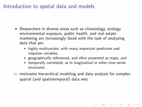
I Researchers in diverse areas such as climatology, ecology,environmental exposure, public health, and real estatemarketing are increasingly faced with the task of analyzingdata that are:

I highly multivariate, with many important predictors andresponse variables,

I geographically referenced, and often presented as maps, andI temporally correlated, as in longitudinal or other time series

structures.

⇒ motivates hierarchical modeling and data analysis for complexspatial (and spatiotemporal) data sets.

Introduction (cont’d)

Example: In an epidemiological investigation, we might wish toanalyze lung, breast, colorectal, and cervical cancer rates

I by county and year in a particular state

I with risk factors, e.g., age, race, smoking, mammography, andother important screening and staging information alsoavailable at some level.

Introduction (cont’d)

Example: In a meteorological investigation, we might wish toanalyze temperature and precipitation data

I with say hourly or daily measurements at a network ofmonitoring station

I with a mean surface that reflects say elevation, perhaps atrend in elevation

Introduction (cont’d)

Example: In an ecological setting, we may be interested in thepoint pattern of locations for say two different species, e.g., junipertrees and pine trees

I with geo-coded locations for each of the trees and a labelindicating which species

I and environmental features to explain species distribution

I possibly collected over time in order to see change, evolution,diffusion of the patterns

Existing spatial statistics booksI Cressie (1990, 1993): the legendary “bible” of spatial

statistics, but rather high mathematical level, lacks modernhierarchical modeling/computing

I Update is Cressie and Wikle (2011) Statistics forSpatio-temporal Data

I The Handbook of Spatial Statistics (Gelfand et al., 2010)

I Wackernagel (1998): terse; only geostatistics

I Chiles and Delfiner (1999): only geostatistics

I Stein (1999a): theoretical treatise on kriging

I So, of course Banerjee, Carlin, and Gelfand (2014)!

I More descriptive presentations: Bailey and Gattrell (1995),Fotheringham and Rogerson (1994), or Haining (1990).

Our primary focus is on modeling, computing, and dataanalysis.

Types of spatial data

I point-referenced data, where Y (s) is a random vector at aselected location s ∈ <r and s varies continuously over D, afixed subset of <r ;

I areal data, where D is again a fixed subset (of regular orirregular shape), but now partitioned into a finite number ofareal units with well-defined boundaries and observations areassociated with the areal units; discrete spatial data

I point pattern data, where now the set of locations in D isitself random; its index set gives the locations of randomevents that are the spatial point pattern. Can assign Y (s) = 1for all s ∈ D (indicating occurrence of the event), or possiblyassign labels to the points (producing a marked point patternprocess).

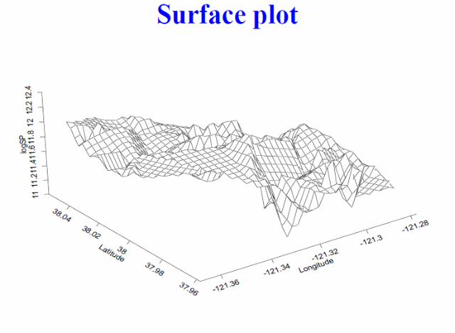
Point-level (geostatistical) data

< 12.9 12.9 - 13.7 13.7 - 14.6 14.6 - 15.5 15.5 - 16.4 16.4 - 17.3 17.3 - 18.1 18.1 - 19 19 - 19.9 > 19.9

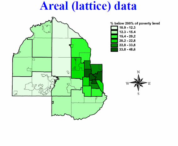
Notes on areal data

I This figure is an example of a choropleth map, which usesshades of color (or greyscale) to classify values into a fewbroad classes, like a histogram

I From the choropleth map we know which regions are adjacentto (share a boundary or a corner) which other regions.

I Thus the “sites” s ∈ D in this case are actually the regions (orblocks) themselves, which we will denote not by si but byBi , i = 1, . . . , n.

A few words on cartography

I The earth is round! So (longitude, latitude) 6= (x , y)!

I A map projection is a systematic representation of all or partof the surface of the earth on a plane.

I Theorem: The sphere cannot be flattened onto a planewithout distortion

I Instead, use an intermediate surface that can be flattened.The sphere is first projected onto the this developable surface,which is then laid out as a plane.

I The three most commonly used surfaces are the cylinder, thecone, and the plane itself.

I Using different orientations of these surfaces leads to differentclasses of map projections...

cont.

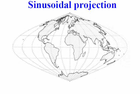
Writing (longitude, latitude) as (λ, θ), projections are

x = f (λ, φ), y = g(λ, φ) ,

where f and g are chosen based upon properties our map mustpossess. This sinusoidal projection preserves area.

cont.

While no projection preserves distance (Gauss’ TheoremaEggregium in differential geometry), this famous conformal(angle-preserving) projection distorts badly near the poles.

Basics of Point-Referenced Data Models

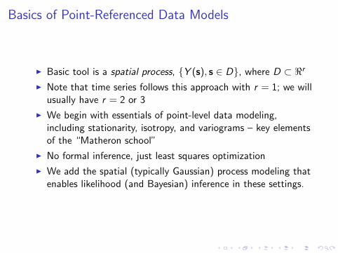
I Basic tool is a spatial process, Y (s), s ∈ D, where D ⊂ <r

I Note that time series follows this approach with r = 1; we willusually have r = 2 or 3

I We begin with essentials of point-level data modeling,including stationarity, isotropy, and variograms – key elementsof the “Matheron school”

I No formal inference, just least squares optimization

I We add the spatial (typically Gaussian) process modeling thatenables likelihood (and Bayesian) inference in these settings.

Stationarity

Suppose our spatial process has a mean, µ (s) = E (Y (s)), andthat the variance of Y (s) exists for all s ∈ D.

I The process is said to be strictly stationary (also calledstrongly stationary) if, for any given n ≥ 1, any set of n sitess1, . . . , sn and any h ∈ <r , the distribution of(Y (s1) , . . . ,Y (sn)) is the same as that of(Y (s1 + h) , . . . ,Y (sn + h)).

I A less restrictive condition is given by weak stationarity (alsocalled second-order stationarity): A process is weaklystationary if µ (s) ≡ µ and Cov (Y (s) ,Y (s + h)) = C (h) forall h ∈ <r such that s and s + h both lie within D.

Notes on Stationarity

I Weak stationarity says that the covariance between the valuesof the process at any two locations s and s + h can besummarized by a covariance function C (h) (sometimes calleda covariogram), and this function depends only on theseparation vector h.

I Note that with all variances assumed to exist, strongstationarity implies weak stationarity.

I The converse is not true in general, but it does hold forGaussian processes

Gaussian processes

I The process Y (s) is said to be Gaussian, i.e., a Gaussianprocess, a GP, if, for any n ≥ 1 and any set of sitess1, s2, ..., sn, Y = (Y (s1),Y (s2), ...,Y (sn)) has amultivariate normal distribution.

I How do we create the multivariate normal distribution?

I We specify a mean function µ(s) and a “valid” covariancefunction C (s, s′) ≡ cov(Y (s),Y (s′))

I Then, Y ∼ N(µ,Σ) where µi = µ(si ) and Σij = C (si , sj).

I The mean function is usually some sort of regressionspecification

I The covariance function is specified through a few parameterssay θ, so we have Σ(θ) providing structured dependence

Why do we love GPs?I Restriction to Gaussian processes enables several advantages.I Convenient specification: the mean function and the

covariance function determine all distributions.I Convenient distribution theory. Joint marginal and conditional

distributions are all immediately obtained from standardtheory given the mean and covariance structure.

I With hierarchical modeling, a Gaussian process assumption forspatial random effects at the second stage of the model alignswith the way independent random effects with variancecomponents are customarily introduced in foregoing linear orgeneralized linear mixed models.

I Technically, with Gaussian processes and stationary models,strong stationarity is equivalent to weak stationarity

I It is difficult to criticize a Gaussian assumption. We haveY = (Y (s1),Y (s2), ...,Y (sn)), a single realization from ann-dimensional distribution. With a sample size of one, howcan we criticize any multivariate distributional specification?

Wait a minute!

I Strictly speaking this last assertion is not quite true with aGaussian process model.

I That is, the joint distribution is a multivariate normal withmean, say, 0, and a covariance matrix that is a parametricfunction of the parameters in the covariance function.

I As n grows large enough, the effective sample size will alsogrow.

I By linear transformation we can obtain a set of approximatelyuncorrelated variables through which the adequacy of thenormal assumption might be studied.

Variograms

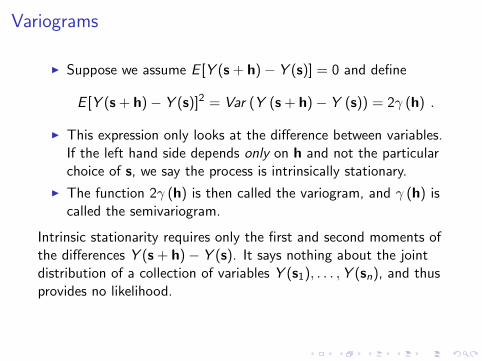
I Suppose we assume E [Y (s + h)− Y (s)] = 0 and define

E [Y (s + h)− Y (s)]2 = Var (Y (s + h)− Y (s)) = 2γ (h) .

I This expression only looks at the difference between variables.If the left hand side depends only on h and not the particularchoice of s, we say the process is intrinsically stationary.

I The function 2γ (h) is then called the variogram, and γ (h) iscalled the semivariogram.

Intrinsic stationarity requires only the first and second moments ofthe differences Y (s + h)− Y (s). It says nothing about the jointdistribution of a collection of variables Y (s1), . . . ,Y (sn), and thusprovides no likelihood.

Relationship between C (h) and γ(h)

I We have

2γ(h) = Var (Y (s + h)− Y (s))

= Var(Y (s + h)) + Var(Y (s))− 2Cov(Y (s + h),Y (s))

= C (0) + C (0)− 2C (h)

= 2 [C (0)− C (h)] .

I Thus,γ (h) = C (0)− C (h) .

I So given C , we are able to determine γ.

I But what about the converse: can we recover C from γ?...

Relationship between C (h) and γ(h)

I In the relationship γ (h) = C (0)− C (h) we can ± a constanton the right side so C (h) is not identified

I Usually, we want the spatial process to be ergodic. Otherwise,no good inference properties.

I This means C (h)→ 0 as ||h|| → ∞, where ||h|| is the lengthof h.

I If so, then, as ||h|| → ∞, γ(h)→ C (0)

I Hence, C (h) = C (0)− γ(h) and both terms on the right sidedepend on γ(·) So C (h) is now well defined given γ(h)

So, previous slide showed that weak stationarity implies intrinsicstationarity. The converse is not true in general but is with theabove condition on γ(h)

Isotropy

I If the semivariogram γ (h) depends upon the separation vectoronly through its length ||h||, then we say that the process isisotropic.

I For an isotropic process, γ (h) is a real-valued function of aunivariate argument, and can be written as γ (||h||).

I If the process is intrinsically stationary and isotropic, it is alsocalled homogeneous.

Isotropic processes are popular because of their simplicity,interpretability, and because a number of relatively simpleparametric forms are available as candidates for C (and γ).Denoting ||h|| by t for notational simplicity, the next two tablesprovide a few examples...

Some common isotropic covariograms

Model Covariance function, C (t)

Linear C (t) does not exist

Spherical C (t) =

0 if t ≥ 1/φ

σ2[1− 3

2φt + 12 (φt)3

]if 0 < t ≤ 1/φ

τ2 + σ2 if t = 0

Exponential C (t) =

σ2 exp(−φt) if t > 0τ2 + σ2 if t = 0

Poweredexponential

C (t) =

σ2 exp(−|φt|p) if t > 0

τ2 + σ2 if t = 0Maternat ν = 3/2

C (t) =

σ2 (1 + φt) exp(−φt) if t > 0

τ2 + σ2 if t = 0

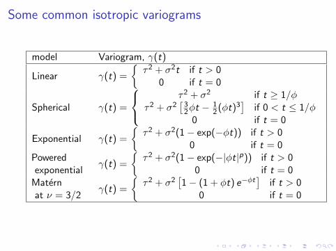
Some common isotropic variograms

model Variogram, γ(t)

Linear γ(t) =

τ2 + σ2t if t > 0

0 if t = 0

Spherical γ(t) =

τ2 + σ2 if t ≥ 1/φ

τ2 + σ2[

32φt −

12 (φt)3

]if 0 < t ≤ 1/φ

0 if t = 0

Exponential γ(t) =

τ2 + σ2(1− exp(−φt)) if t > 0

0 if t = 0Poweredexponential

γ(t) =

τ2 + σ2(1− exp(−|φt|p)) if t > 0

0 if t = 0Maternat ν = 3/2

γ(t) =

τ2 + σ2

[1− (1 + φt) e−φt

]if t > 0

0 if t = 0

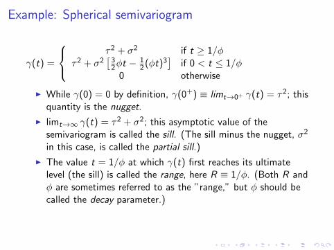
Example: Spherical semivariogram

γ(t) =

τ2 + σ2 if t ≥ 1/φ

τ2 + σ2[

32φt −

12 (φt)3

]if 0 < t ≤ 1/φ

0 otherwise

I While γ(0) = 0 by definition, γ(0+) ≡ limt→0+ γ(t) = τ2; thisquantity is the nugget.

I limt→∞ γ(t) = τ2 + σ2; this asymptotic value of thesemivariogram is called the sill. (The sill minus the nugget, σ2

in this case, is called the partial sill.)

I The value t = 1/φ at which γ(t) first reaches its ultimatelevel (the sill) is called the range, here R ≡ 1/φ. (Both R andφ are sometimes referred to as the ”range,” but φ should becalled the decay parameter.)

The exponential model

I The sill is only reached asymptotically, meaning that strictlyspeaking, the range is infinite.

I To define an ”effective range”, for t > 0, we see that ast →∞, γ(t)→ τ2 + σ2 which would become C (0).

I Again,

C (t) =

τ2 + σ2 if t = 0

σ2 exp(−φt) if t > 0.

I Then the correlation between two points distance t apart isexp(−φt);

I We define the effective range, t0, as the distance at which thiscorrelation = 0.05. Setting exp(−φt0) equal to this value weobtain t0 ≈ 3/φ, since log(0.05) ≈ −3.

cont.

I We introduce an intentional discontinuity at 0 for both thecovariance function and the variogram.

I To clarify why, suppose we write the error at s in our spatialmodel as w(s) + ε(s) where w(s) is a mean 0 process withcovariance function σ2ρ(t) and ε(s) is so-called “white noise”,i.e., the ε(s) are i.i.d. N(0, τ2)

I Then, we can compute var(w(s) + ε(s)) = σ2 + τ2

I And, we can computeCov(w(s) + ε(s),w(s + h) + ε(s + h)) = σ2ρ(||h||)

I So, the form of C (t) shows why the nugget τ2 is often viewedas a “nonspatial effect variance,” and the partial sill (σ2) isviewed as a “spatial effect variance.”

The Matern Correlation Function

I The Matern is a very versatile family:

C (t) =

σ2

2ν−1Γ(ν)(2√νtφ)νKν(2

√(ν)tφ) if t > 0

τ2 + σ2 if t = 0

Kν is the modified Bessel function of order ν (computationallytractable in C/C++ or geoR)

I ν is a smoothness parameter:I ν = 1/2⇒ exponential; ν →∞⇒ Gaussian; ν = 3/2⇒

convenient closed form for C (t), γ(t)I in two-dimensions, the greatest integer in ν indicates the

number of times process realizations will be mean-squaredifferentiable.

A bit more on covariance functions

I To be a valid covariance function the function must bepositive definite

I Whether a function is positive definite or not can dependupon dimension

I c is a valid covariance functions if and only if it is thecharacteristic function of a symmetric about 0 randomvariable (Bochner’s Theorem), i.e., c(h) =

∫cos(wTh)G (dw)

I Fourier transform, spectral distribution, spectral density

I In principle, the inversion formula could be used to check ifc(h) is valid

Constructing valid covariance functions

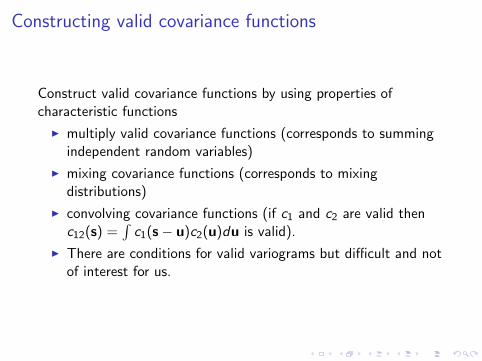
Construct valid covariance functions by using properties ofcharacteristic functions

I multiply valid covariance functions (corresponds to summingindependent random variables)

I mixing covariance functions (corresponds to mixingdistributions)

I convolving covariance functions (if c1 and c2 are valid thenc12(s) =

∫c1(s− u)c2(u)du is valid).

I There are conditions for valid variograms but difficult and notof interest for us.

Variogram model fitting

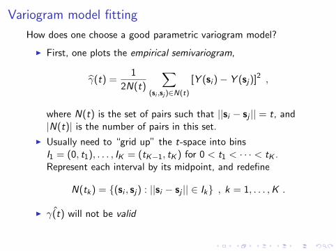
How does one choose a good parametric variogram model?

I First, one plots the empirical semivariogram,

γ(t) =1

2N(t)

∑(si ,sj )∈N(t)

[Y (si )− Y (sj)]2 ,

where N(t) is the set of pairs such that ||si − sj || = t, and|N(t)| is the number of pairs in this set.

I Usually need to “grid up” the t-space into binsI1 = (0, t1), . . . , IK = (tK−1, tK ) for 0 < t1 < · · · < tK .Represent each interval by its midpoint, and redefine

N(tk) = (si , sj) : ||si − sj || ∈ Ik , k = 1, . . . ,K .

I ˆγ(t) will not be valid

Variogram model fitting (cont’d)

I This method of moments estimator (analogue of the usualsample variance s2) has problems:

I It will be sensitive to outliers

I A sample average of squared differences can be badly behaved.

I It uses data differences, rather than the data itself.

I The components of the sum will be dependent within andacross bins, and N(tk) will vary across bins.

I Informally, one plots γ(t), and then an appropriately shapedtheoretical variogram is fit by eye or by trial and error tochoose the nugget, sill, and range.

I Formal fitting using least squares, weighted least squares orgeneralized least squares

Anisotropy

I Isotropy implies circular contours in terms of decay in spatialdependence, i.e., association doesn’t depend upon direction

I Stationarity is more general in that it allows association todepend upon the separation vector between locations (i.e.,direction and distance).

I As special case is geometric anisotropy, where

c(s− s′) = σ2ρ((s− s′)TB(s− s′)) .

I B is positive definite with ρ a valid correlation function.

I Since the equation (s− s′)TB(s− s′) = k is an ellipse in2-dim space, spatial dependence is constant on ellipses. Thismeans dependence depends on direction. In particular, thecontour corresponding to ρ = .05 provides the effective rangein each spatial direction.

Anisotropy (cont’d)

I Both geometric anisotropy and product geometric anisotropyare special cases of range anisotropy (Zimmerman, 1993)

I Suggests we might also define sill anisotropy: Given avariogram γ(h), what is the behavior of γ(ch/ ‖h‖) asc →∞? Does it depend upon h

I nugget anisotropy: Given a variogram γ(h), what is thebehavior of γ(ch/ ‖h‖) as c → 0? Does it depend upon h.

Exploration of Spatial Data

I First step in analyzing data

I First Law of Geostatistics: Mean + Error

I Mean: first-order behavior

I Error: second-order behavior (covariance function)

I Wide variety of EDA tools to examine both first and secondorder behavior (Cressie’s book)

I Crucial point: the spatial structure you might see in the Y (s)surface need not look anything like the spatial structure in theresidual surface, after you have fit an explanatory model forthe mean, say µ(s).

E ((Y (s)− µ(s))(Y (s′)− µ(s′)) = E ((Y (s)− µ)(Y (s′)− µ)

+(µ− µ(s))(µ− µ(s′))

Classical spatial prediction (Kriging)

I Named in honor of D.G. Krige, a South African miningengineer whose seminal work on empirical methods forgeostatistical data inspired the general approach

I Optimal spatial prediction: given observations of a randomfield Y = (Y (s1) , . . . ,Y (sn))′, predict the variable Y at asite s0 where it has not been observed

I Under squared error loss, the best linear prediction minimizesE [Y (s0)− (

∑`iY (si ) + δ0)]2 over δ0 and `i .

I Under intrinsic stationarity, adopting unbiasedness, δ0 dropsout. Obviously, Y is not best.

I With an estimate of γ, one immediately obtains the ordinarykriging estimate.

I No distributional assumptions are required for the Y (si ).

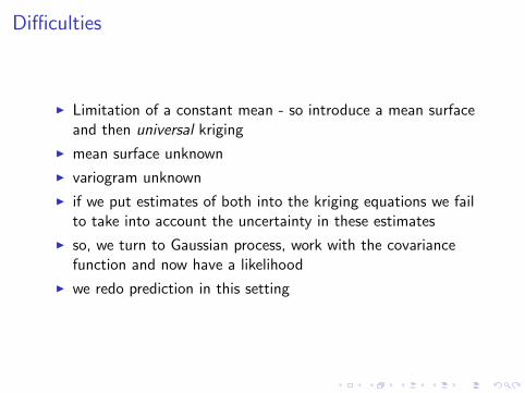
Difficulties

I Limitation of a constant mean - so introduce a mean surfaceand then universal kriging

I mean surface unknown

I variogram unknown

I if we put estimates of both into the kriging equations we failto take into account the uncertainty in these estimates

I so, we turn to Gaussian process, work with the covariancefunction and now have a likelihood

I we redo prediction in this setting

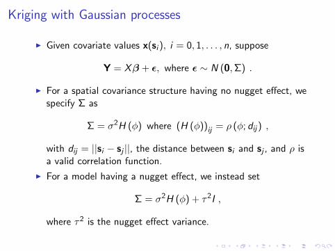
Kriging with Gaussian processes

I Given covariate values x(si ), i = 0, 1, . . . , n, suppose

Y = Xβ + ε, where ε ∼ N (0,Σ) .

I For a spatial covariance structure having no nugget effect, wespecify Σ as

Σ = σ2H (φ) where (H (φ))ij = ρ (φ; dij) ,

with dij = ||si − sj ||, the distance between si and sj , and ρ isa valid correlation function.

I For a model having a nugget effect, we instead set

Σ = σ2H (φ) + τ2I ,

where τ2 is the nugget effect variance.

Kriging with Gaussian processes

I We seek the function g (y) that minimizes the mean-squared

prediction error, E[(Y (s0)− g (y))2 y

], i.e., we work with

the conditional distribution of Y (s0)|yI It is well known that the (posterior) mean minimizes expected

squared error loss.

I So, it must be that the predictor g(y) that minimizes theerror is the conditional expectation, E (Y (s0)|y).

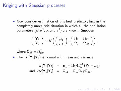
Kriging with Gaussian processes

I Now consider estimation of this best predictor, first in thecompletely unrealistic situation in which all the populationparameters (β, σ2, φ, and τ2) are known. Suppose(

Y1

Y2

)∼ N

((µ1

µ2

),

(Ω11 Ω12

Ω21 Ω22

)),

where Ω21 = ΩT12.

I Then f (Y1|Y2) is normal with mean and variance

E [Y1|Y2] = µ1 + Ω12Ω−122 (Y2 − µ2)

and Var [Y1|Y2] = Ω11 − Ω12Ω−122 Ω21 .

Kriging with Gaussian processes

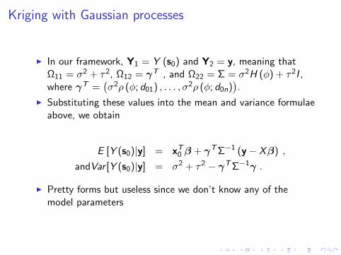
I In our framework, Y1 = Y (s0) and Y2 = y, meaning thatΩ11 = σ2 + τ2, Ω12 = γT , and Ω22 = Σ = σ2H (φ) + τ2I ,where γT =

(σ2ρ (φ; d01) , . . . , σ2ρ (φ; d0n)

).

I Substituting these values into the mean and variance formulaeabove, we obtain

E [Y (s0)|y] = xT0 β + γTΣ−1 (y− Xβ) ,

andVar [Y (s0)|y] = σ2 + τ2 − γTΣ−1γ .

I Pretty forms but useless since we don’t know any of themodel parameters

Kriging with Gaussian processes

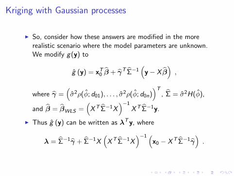
I So, consider how these answers are modified in the morerealistic scenario where the model parameters are unknown.We modify g(y) to

g (y) = xT0 β + γT Σ−1(y− X β

),

where γ =(σ2ρ(φ; d01), . . . , σ2ρ(φ; d0n)

)T, Σ = σ2H(φ),

and β = βWLS =(XT Σ−1X

)−1XT Σ−1y.

I Thus g (y) can be written as λTy, where

λ = Σ−1γ + Σ−1X(XT Σ−1X

)−1 (x0 − XT Σ−1γ

).

Kriging with Gaussian processes

I If X (s0) is unobserved, we can still do the spatial prediction

I We estimate X (s0) and Y (s0) jointly by iterating between theformula for g(y) and a corresponding one for x0, namely

x0 = XTλ ,

which arises simply by multiplying both sides of the previousequation by XT and simplifying.

I This is essentially an EM (expectation-maximization)algorithm, with the calculation of x0 being the E step and theupdating of λ being the M step.

I In the classical framework, restricted maximum likelihood(REML) estimates are often plugged in above and have someoptimal properties.