Cavanaugh 2011 Environmental Controls of Santa Barbara Kelp
17
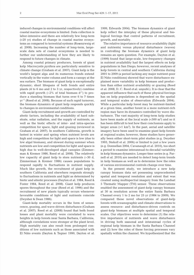
MARINE ECOLOGY PROGRESS SERIES Mar Ecol Prog Ser Vol. 429: 1–17, 2011 doi: 10.3354/meps09141 Published May 16 INTRODUCTION Climate-related changes in the oceans appear to be accelerating: oceans are becoming warmer and more acidic, nutrient distributions are changing, and, in some regions such as the Northeast Pacific, the fre- quency and intensity of large storms are increasing (e.g. Easterling et al. 2000, Behrenfeld et al. 2006, Doney et al. 2009). Many marine ecosystems have displayed dramatic responses to recent fluctuations in climate, and accumulating evidence suggests that coastal marine ecosystems are especially vulnerable to the effects of climate change (e.g. Harley et al. 2006, Przeslawski et al. 2008, Hoegh-Guldberg & Bruno 2010). However, our understanding of how climate- © Inter-Research 2011 · www.int -res.com *Email: [email protected] .edu FEATURE ARTICLE Environmental controls of giant-kelp biomass in the Santa Barbara Channel, California Kyle C. Cavanaugh 1, *, David A. Siegel 1, 2 , Daniel C. Reed 3 , Philip E. Dennison 4 1 Earth Research Institute, 2 Department of Geography , and 3 Marine Science Institute, University of California, Santa Barbara, Calif ornia 9310 6, USA 4 Department of Geography , University of Utah, Salt Lake City, Utah 84112, USA ABSTRACT: Synthesizing long-term observations at multiple scales is vital for understanding the environ- mental drivers of ecosystem dynamics. We assessed the role of several environmental drivers in explaining temporal and spatial patterns in the abundance of giant kelp Macrocystis pyrifera in the Santa Barbara Channel between 1984 and 2009. We developed a novel method for estimating the canopy biomass of giant kelp from Landsat 5 Thematic Mapper satellite imagery, which allowed us to examine the dynamics of giant-kelp biomass on spatial scales ranging from 100s of m 2 to 100s of km 2 and temporal scales ranging from several weeks to 25 yr. Comparisons of changes in canopy biomass with oceanographic and climatic data revealed that winter losses of regional kelp canopy biomass were positively correlated with significant wave height (r 2 = 0.50), while spring recoveries were negatively correlated with sea surface temperature (r 2 = 0.30; used as a proxy for nutrient availability). On interannual timescales, regional kelp-canopy biomass lagged the variations in wave heights, sea surface tem- peratures, and the North Pacific Gyre Oscillation index by 3 yr, indicating that these factors affect cycles of kelp recruitment and mortality. Results from cluster analysis showed that the response of kelp biomass to environmental conditions varied among different sub- regions of the Santa Barbara Channel. The dynamics of kelp biomass in exposed regions were related to wave disturbance, while kelp dynamics in sheltered regions tracked sea surface temperatures more closely. These results depict a high level of regional hetero- geneity in the biomass dynamics of this important foundation species. KEY WORDS: Giant k elp · Spatial and temporal vari- abilit y · Dist urban ce · Remote sensi ng · Long- term data Resale or republication not permitted without written consent of the publisher Canopy biomass of Macrocystis pyrifera (top) can be quanti- fied from Landsat 5 imagery (bottom). Photo: Stuart Halewood O PE N EN A CCESS CESS
-
Upload
mbcmillerbiology -
Category
Documents
-
view
219 -
download
0
Transcript of Cavanaugh 2011 Environmental Controls of Santa Barbara Kelp

8/3/2019 Cavanaugh 2011 Environmental Controls of Santa Barbara Kelp
http://slidepdf.com/reader/full/cavanaugh-2011-environmental-controls-of-santa-barbara-kelp 1/17
MARINE ECOLOGY PROGRESS SERIES
Mar Ecol Prog Ser
Vol. 429: 1–17, 2011
doi: 10.3354/meps09141Published May 16
INTRODUCTION
Climate-related changes in the oceans appear to be
accelerating: oceans are becoming warmer and moreacidic, nutrient distributions are changing, and, in
some regions such as the Northeast Pacific, the fre-
quency and intensity of large storms are increasing
(e.g. Easterling et al. 2000, Behrenfeld et al. 2006,
Doney et al. 2009). Many marine ecosystems have
displayed dramatic responses to recent fluctuations in
climate, and accumulating evidence suggests that
coastal marine ecosystems are especially vulnerable to
the effects of climate change (e.g. Harley et al. 2006,
Przeslawski et al. 2008, Hoegh-Guldberg & Bruno
2010). However, our understanding of how climate-
© Inter-Research 2011 · www.int-res.com*Email: [email protected]
FEATURE ARTICLE
Environmental controls of giant-kelp biomass inthe Santa Barbara Channel, California
Kyle C. Cavanaugh1,*, David A. Siegel1, 2, Daniel C. Reed3, Philip E. Dennison4
1Earth Research Institute, 2Department of Geography, and 3Marine Science Institute, University of California, Santa Barbara,
California 93106, USA4Department of Geography, University of Utah, Salt Lake City, Utah 84112, USA
ABSTRACT: Synthesizing long-term observations at
multiple scales is vital for understanding the environ-
mental drivers of ecosystem dynamics. We assessedthe role of several environmental drivers in explaining
temporal and spatial patterns in the abundance of
giant kelp Macrocystis pyrifera in the Santa Barbara
Channel between 1984 and 2009. We developed a
novel method for estimating the canopy biomass ofgiant kelp from Landsat 5 Thematic Mapper satellite
imagery, which allowed us to examine the dynamics of
giant-kelp biomass on spatial scales ranging from 100s
of m2 to 100s of km2 and temporal scales ranging from
several weeks to 25 yr. Comparisons of changes in
canopy biomass with oceanographic and climatic datarevealed that winter losses of regional kelp canopy
biomass were positively correlated with significant
wave height (r2 = 0.50), while spring recoveries were
negatively correlated with sea surface temperature
(r2 = 0.30; used as a proxy for nutrient availability). On
interannual timescales, regional kelp-canopy biomasslagged the variations in wave heights, sea surface tem-
peratures, and the North Pacific Gyre Oscillation index
by 3 yr, indicating that these factors affect cycles of
kelp recruitment and mortality. Results from cluster
analysis showed that the response of kelp biomass to
environmental conditions varied among different sub-regions of the Santa Barbara Channel. The dynamics
of kelp biomass in exposed regions were related to
wave disturbance, while kelp dynamics in sheltered
regions tracked sea surface temperatures more closely.
These results depict a high level of regional hetero-geneity in the biomass dynamics of this important
foundation species.
KEY WORDS: Giant kelp · Spatial and temporal vari-
ability · Disturbance · Remote sensing · Long-term data
Resale or republication not permitted without written consent of the publisher
Canopy biomass of Macrocystis pyrifera (top) can be quanti-fied from Landsat 5 imagery (bottom).
Photo: Stuart Halewood
OPENEN ACCESSCESS
8/3/2019 Cavanaugh 2011 Environmental Controls of Santa Barbara Kelp
http://slidepdf.com/reader/full/cavanaugh-2011-environmental-controls-of-santa-barbara-kelp 2/17
Mar Ecol Prog Ser 429: 1–17, 2011
induced changes in environmental conditions will affect
coastal marine ecosystems is limited. Data collection is
labor-intensive and there are relatively few long-term
(>20 yr) studies of change in coastal marine ecosys-
tems as compared to terrestrial systems (Rosenzweig et
al. 2008). Increasing the number of long-term, large-scale data sets of coastal ecosystems is needed to
further our understanding of how they are likely to
respond to future changes in climate.
Among coastal primary producers, forests of giant
kelp Macrocystis pyrifera are particularly sensitive to
climate change (Graham et al. 2007). Giant kelp is the
world’s largest alga and its numerous fronds extend
vertically in the water column and form a canopy at the
sea surface. The biomass of giant kelp is exceptionally
dynamic; short lifespans of both fronds and entire
plants (4 to 6 mo and 2 to 3 yr, respectively) combine
with rapid growth (~2% of total biomass d–1) to pro-
duce a standing biomass that turns over 6 to 7 timesyr–1 (Reed et al. 2008). Because of such rapid turnover,
the biomass dynamics of giant kelp responds quickly
to changes in environmental conditions.
Giant-kelp recruitment and growth are controlled by
abotic factors, including the availability of hard sub-
strate, solar radiation, and the supply of nutrients, as
well as the biotic effects of inter- and intra-species
competition for space, light and grazing (reviewed in
Graham et al. 2007). In southern California, growth is
fastest in winter and spring when nutrient levels are
high and competition for light and space is low (due to
low algal biomass), and slowest during summer when
nutrients are low and competition for light and space is
high due to well-developed algal canopies (Zimmer-
man & Kremer 1986, Reed et al. 2008). The relatively
low capacity of giant kelp to store nutrients (~30 d,
Zimmerman & Kremer 1986) causes populations to
respond rapidly to fluctuations in nutrient supply.
Much like growth, the recruitment of giant kelp in
southern California and elsewhere responds strongly
to fluctuations in nutrients and light as determined by
biotic and abiotic processes (Dayton et al. 1984, Reed &
Foster 1984, Reed et al. 2008). Giant kelp produces
spores throughout the year (Reed et al. 1996) and the
recruitment of new plants typically occurs wheneverfavorable conditions of light and nutrients coincide
(Deysher & Dean 1986).
Giant-kelp mortality occurs in the form of senes-
cence, grazing, and wave-driven disturbance (Graham
et al. 2007). Reed et al. (2008) found that both frond
losses and plant mortality were correlated to wave
heights in kelp forests near Santa Barbara, California,
although correlations were stronger at the plant level.
High mortality can also result from prolonged con-
ditions of low nutrients such as those associated with
El Niño events (Dayton & Tegner 1990, Dayton et al.
1999, Edwards 2004). The biomass dynamics of giant
kelp reflect the interplay of these physical and bio-
logical forcings that control patterns of recruitment,
growth, and mortality.
The relative importance of resource availability (light
and nutrients) versus physical disturbance (waves)in controlling the biomass dynamics of giant kelp
remains an open question. For example, Dayton et al.
(1999) found that large-scale, low-frequency changes
in nutrient availability had the largest effects on kelp
populations in San Diego; however, recent analyses of
kelp forests in central and southern California during
2001 to 2009 (a period lacking any major nutrient-poor
El Niño conditions) showed that wave disturbance ex-
plained more variability in kelp biomass and produc-
tion than either nutrient availability or grazing (Reed
et al. 2008, D. C. Reed et al. unpubl.). It is clear that the
apparent influence that each of these physical forcings
has on kelp populations is dependent on the spatialand temporal scales of observation (Edwards 2004).
While a particular kelp forest may be nutrient-limited
at a given time, another forest in a more nutrient-rich
region may have its dynamics controlled by wave dis-
turbance. The vast majority of long-term kelp studies
have been made at the local scale (<500 m2) and so it
has been difficult to test how their conclusions apply to
larger areas (>1 km2). In the past, aerial and satellite
imagery have been used to examine giant kelp forests
at regional scales; however, these studies have gener-
ally been either short-term pilot studies (e.g. Deysher
1993, Stekoll et al. 2006) or limited to just a few years
(e.g. Donnellan 2004, Cavanaugh et al. 2010), too short
a period to examine interannual-to-decadal variability
in kelp biomass dynamics. Longer time series (e.g. Par-
nell et al. 2010) are needed to detect long-term trends
in kelp biomass as well as to determine how the roles
of various environmental controls change over time.
In the present study, we introduce a new kelp
canopy biomass data set possessing unprecedented
spatial and temporal resolution and extent that was
created using multispectral imagery from the Landsat
5 Thematic Mapper (TM) sensor. These observations
enabled the assessment of giant-kelp canopy biomass
at 30 m resolution across the entire Santa BarbaraChannel every 1 to 2 mo for 25 yr (1984 to 2009). We
compared these novel observations of giant-kelp
forests with oceanographic and climate observations to
assess resource- and disturbance-driven controls on
giant-kelp biomass at multiple spatial and temporal
scales. Our objectives were to determine (1) the rela-
tive importance of nutrients and wave disturbance
in driving both seasonal and interannual cycles of
regional kelp biomass in the Santa Barbara Channel
and (2) how the roles of these forcing processes vary
spatially within the channel. We hypothesized that the
2

8/3/2019 Cavanaugh 2011 Environmental Controls of Santa Barbara Kelp
http://slidepdf.com/reader/full/cavanaugh-2011-environmental-controls-of-santa-barbara-kelp 3/17
Cavanaugh et al.: Environmental controls of giant-kelp biomass
negative effects of wave disturbance and nutrient
limitation on giant-kelp biomass vary greatly in space
and time due to the highly dynamic environmental
conditions of the Santa Barbara Channel. We showed
that kelp biomass was significantly negatively related
to wave heights and sea surface temperatures (SST;a proxy for nutrient levels) at seasonal timescales.
Interannual relationships were more complex as kelp
biomass lagged wave heights, SST, and the North
Pacific Gyre Oscillation (NPGO) climate index by 3 yr.
We also demonstrated that these dependencies varied
between distinct subregions within the Santa Barbara
Channel.
MATERIALS AND METHODS
Study site. We tracked giant-kelp canopy biomass
across the entire Santa Barbara Channel from 1984 to2009. The study area included the coastline from Pismo
Beach, CA to Oxnard, CA and each of the northern
Channel Islands (Fig. 1). Giant kelp in this region is
found primarily on shallow rocky reefs that are distrib-
uted in patches. The light-attenuation properties of the
waters in the channel limit giant kelp to depths <30 m.
The Santa Barbara Channel experiences pronounced
seasonal cycles in SST, nutrient conditions, and wave
energy (Harms & Winant 1998, Otero & Siegel 2004).
During the winter, large storms in the North Pacific
create large northwesterly swells (>4 m) that enter the
Santa Barbara Channel. Wave energy from these
storms is a major source of giant-kelp mortality in the
region (Reed et al. 2008). Nutrient levels are relatively
high (~3 µmol l–1
nitrate, Fram et al. 2008) in the winteras a deepening of the mixed layer entrains nutrients
into surface waters (McPhee-Shaw et al. 2007). SST
and nutrients (specifically nitrate and nitrite) are
inversely correlated in the Santa Barbara Channel (r2 =
0.87, Fram et al. 2008) and elsewhere in southern Cal-
ifornia. Studies done to date indicate that the growth of
giant kelp in southern California is more commonly
limited by low nutrients than by high SST (Clenden-
ning & Sargent 1971, North & Zimmerman 1984).
Spring represents a period of transition in surface
wave conditions as the frequency of large northwest-
erly wave events decreases, giving way to smaller
southerly swells (2 to 3 m) that are characteristic ofsummer months (Adams et al. 2008). Nitrate levels
in the nearshore regions generally reach maximums
(>10 µmol l–1, McPhee-Shaw et al. 2007; Fram et al.
2008) during spring months due to coastal upwelling.
During the summer and fall, vertical stratification
increases, creating warmer temperatures and lower
nitrate levels (<1 µmol l–1, Fram et al. 2008). Less
intense southerly swells are common in the summer
months and can affect exposed south-facing coastlines.
The seasonal cycles in resource availability and
physical disturbance are super-imposed on longer
period cycles driven by El Niño-Southern Oscillation,
Pacific Decadal Oscillation (PDO), and NPGO events.
These lower-frequency climate cycles alter seawater
temperatures, nutrient levels, and storm patterns, and
can have dramatic effects on kelp populations (Dayton
et al. 1999, Edwards 2004).
The Santa Barbara Channel also experiences a great
deal of spatial variability in oceanographic conditions.
The region is located at the convergence of the equa-
torward-flowing California Current and the recirculat-
ing Southern California Eddy and Inshore Counter-
current (Hickey 1979). Strong upwelling north of
Point Conception creates cool, nutrient-rich conditions
throughout most of the year, while regions in the east-ern portion of the channel experience warmer, more
nutrient-limited conditions during summer months
(Otero & Siegel 2004). While there is spatial variability
in the SST of the Santa Barbara Channel, the vast
majority of the region’s temporal variability is homoge-
neous across the entire channel (Otero & Siegel 2004,
see ‘Materials and methods–regional physical and cli-
mate data sets’).
Even more dramatic is the spatial variability in wave
exposure. Again, Point Conception represents a natural
boundary: the coastline north of Point Conception is
3
Fig. 1. Landsat 5 Thematic Mapper image displaying studyarea; Point Arguello, Harvest, and Harvest platform buoys;
and Long Term Ecological Research (LTER) diver transects atthe Arroyo Quemado (AQUE) and Mohawk (MOHK) kelp
forests

8/3/2019 Cavanaugh 2011 Environmental Controls of Santa Barbara Kelp
http://slidepdf.com/reader/full/cavanaugh-2011-environmental-controls-of-santa-barbara-kelp 4/17
Mar Ecol Prog Ser 429: 1–17, 2011
exposed to both powerful winter northwest swells as
well as weaker summer southern swells while the
coastline south of Point Conception is sheltered from
northern swells by Point Conception and from south-
ern swells by the Channel Islands (O’Reilly & Guza
1993). The Channel Islands themselves present a myr-iad of exposures, but in general the north sides of the
islands are exposed to northwest swells and sheltered
from southern swells, while the opposite is true for the
south-facing sides of the islands. Note that while these
descriptions depict wave exposure in general, the pre-
cise spatial distribution of wave energy along the coast
of our study area depends on the specific direction of a
given swell (Adams et al. 2008). As with SST and nutri-
ents, large, long-period swells affect the entire chan-
nel, but to varying degrees due to the large amount of
spatial variability in wave exposure. Clearly, subtidal
ecosystems of the Santa Barbara Channel such as giant
kelp forests experience physical conditions that varysubstantially in space and time.
Satellite estimation of giant-kelp canopy biomass.
Giant kelp forms a dense floating canopy at the sea
surface that is distinctive when viewed from above. In
our study area, giant kelp is the only canopy-forming
macrophyte in water depths from 5 to 30 m. This
greatly simplifies its quantification from satellite
imagery. The spectral signature of a giant-kelp canopy
is similar to that of photosynthetically active terrestrial
vegetation, namely a high near-infrared and signifi-
cantly lower visible reflectance (Jensen et al. 1980,
Cavanaugh et al. 2010). Water absorbs almost all in-
coming near-infrared energy so kelp canopy is easily
differentiated using its near-infrared reflectance signal.
The Landsat 5 TM sensor has acquired 30 m spatial
resolution multispectral imagery nearly continuously
from 1984 to the present on a 16 d repeat cycle
(Markham et al. 2004). TM obtains data in 7 spectral
bands: blue (450 to 520 nm), green (520 to 600 nm), red
(630 to 690 nm), near-infrared (760 to 900 nm), short-
wave infrared (1500 to 1750 and 2080 to 2350 nm), and
longwave (thermal) infrared (10400 to 12 500 nm)
(http://landsat.gsfc.nasa.gov/about/tm.html). TM data
is stored as 8-bit encoded radiance, with 256 possible
‘brightness values’ representing the range of radiancefor each band. The kelp near-infrared (Band 4) radi-
ance signal, while elevated compared to that of water,
spans only the lowest ~40 brightness values detectable
by TM.Each Landsat scene covers an area170 × 180 km;
the scene we used for the present study included the
entire study area described above (‘Study site’) (Fig. 1).
During preprocessing, Landsat images were geometri-
cally corrected using ground control points and a digi-
tal elevation model to achieve a scene-to-scene regis-
tration accuracy <7.3 m (Lee et al. 2004). We selected
209 relatively cloud-free images that provided us with
coverage of the study area approximately every 2 mo
from April 1984 to September 2009 (http://glovis.usgs.
gov/).
We developed an automated classification and quan-
tification process in order to consistently and effi-
ciently transform the 209 TM images into maps ofkelp canopy biomass. First, a single orthorectified TM
image was atmospherically corrected to apparent
surface reflectance using an atmospheric transmission
model (MODTRAN4; Berk et al. 1998). We used this
corrected image as a reference and standardized the
radiometric signals from all other images to this refer-
ence using 50 targets that were assumed to be spec-
trally stable across the time series (i.e. airport runways,
highways, sand dunes, lakes; Furby & Campbell 2001,
Baugh & Groeneveld 2008). Outliers were manually
removed to reduce the effects of temporal changes in
target reflectance. This ‘target matching’ procedure
accounted for all atmospheric, sensor, and processingdifferences between the scenes and created a time-
series of standardized TM imagery.
We estimated kelp canopy abundance from the cali-
brated TM reflectance data using multiple endmember
spectral mixture analysis (MESMA). Spectral mixture
analysis models the fractional cover of 2 or more ‘end-
members’ within a pixel. Each endmember represents
a pure cover type, and endmembers are assumed to
combine linearly (Adams et al. 1993). Standard spec-
tral mixture analysis uses a uniform set of endmembers
for the entire image. One challenge in the near-shore
marine zone is that the ‘water’ reflectance is influ-
enced by e.g. sun glint, breaking surface waves,
phytoplankton blooms, dissolved organic matter, and
sediment runoff. Since water reflectance is highly
variable in space and time, a single water endmember
cannot be used (Fig. 2A).
Roberts et al. (1998) developed MESMA to allow
endmembers to vary on a per-pixel basis. By selecting
from multiple endmembers for 1 or more cover types,
MESMA can better capture the spectral variability of
the cover type within an image and through time.
MESMA has been extensively used for mapping ter-
restrial vegetation, including aridland vegetation (Okin
et al. 2001), shrublands (Dennison & Roberts 2003a),forests (Youngentob et al. 2011), and salt marsh (Li et
al. 2005).
We modeled pixel reflectance as the linear mixture
of reflectance of 2 endmembers: kelp and water. Thirty
water endmembers were selected from non-kelp-
covered areas within each TM scene using the end-
member selection technique described by Dennison
& Roberts (2003b). A single kelp endmember was
selected by extracting kelp-covered pixel spectra from
each image and finding the single spectrum that fit the
entire library of kelp spectra with the lowest root mean
4
8/3/2019 Cavanaugh 2011 Environmental Controls of Santa Barbara Kelp
http://slidepdf.com/reader/full/cavanaugh-2011-environmental-controls-of-santa-barbara-kelp 5/17
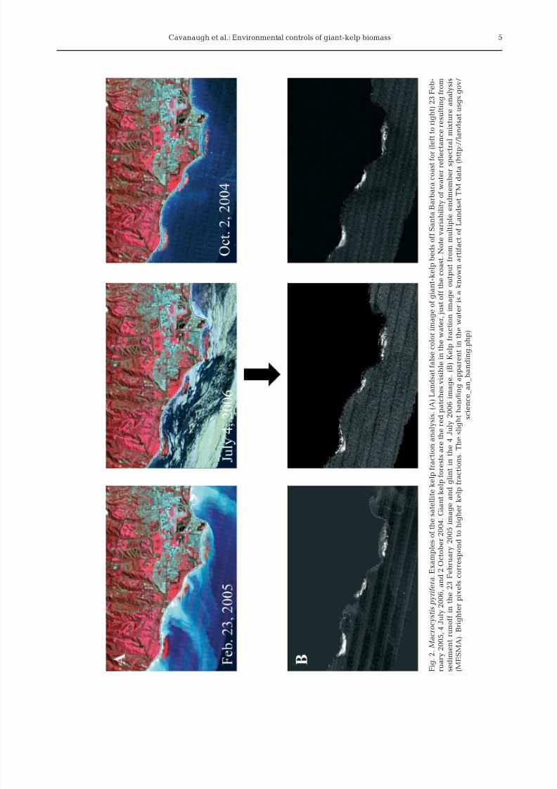
Cavanaugh et al.: Environmental controls of giant-kelp biomass 5
F i g . 2 .
M a c r o c y s t i s p y r i f e r a . E x a m p
l e s o f t h e s a t e l l i t e k e l p f r a c t i o n a n a l y s i s . ( A ) L a n d s a t f a l s e c o l o r i m a g e o f g i a n t - k
e l p b e d s o f f S a n t a B a r b a r a c o a s t f o r ( l e f t
t o r i g h t ) 2 3 F e b -
r u a r y 2 0 0 5 , 4 J u l y 2 0 0 6 , a n d 2 O c t o
b e r 2 0 0 4 . G i a n t k e l p f o r e s t s a r e t h e r e d p a t c h e s v i s i b l e i n t h e w a t e r , j u s t o f f t h e c o a s t . N o t e v a r i a b i l i t y o f w a t e r r e f l e c t a n c e r e s u l t i n g f r o m
s e d i m e n t r u n o f f i n t h e 2 3 F e b r u a r
y 2 0 0 5 i m a g e a n d g l i n t i n t h e 4 J u l y 2 0 0 6 i m a g e . ( B ) K e l p f r a c t i o n i m a g e o u t p u t f r o m
m u l t i p l e e n d m e m b e r s p e c t r a l
m i x t u r e a n a l y s i s
( M E S M A ) . B r i g h t e r p i x e l s c o r r e s p o n d t o h i g h e r k e l p f r a c t i o n s . T h e s l i g h t b a n d i n g a p p a r e n t i n t h e w a t e r i s a k n o w n a r t i f a c t o f L a n d s a t T M d a t a ( h t t p : / / l a n d s a t . u s g s . g o v /
s c
i e n c e_ a n_
b a n d i n g . p h p )

8/3/2019 Cavanaugh 2011 Environmental Controls of Santa Barbara Kelp
http://slidepdf.com/reader/full/cavanaugh-2011-environmental-controls-of-santa-barbara-kelp 6/17
Mar Ecol Prog Ser 429: 1–17, 2011
square error (RMSE) (Dennison & Roberts 2003b). The
pixels in each TM image were then modeled as a 2-
endmember mixture of kelp and each of the 30 water
endmembers. The final model (out of 30) chosen for
each pixel was the model that minimized RMSE when
fit to the spectrum of that pixel. The result of this pro-cess was a measure of the relative fraction of each
pixel that was covered by kelp canopy (Fig. 2B). We
used a kelp fraction minimum threshold of 0.13 to auto-
mate the identification of ‘kelp-covered’ pixels. The
multiple endmember process successfully delineated
kelp canopy extent under a variety of conditions. Fig. 2
provides examples of how our technique retrieved
kelp fractions from images under optimal conditions
(2 October 2004) and for scenes that were contami-
nated by large amounts of sediment runoff (23 Febru-
ary 2005) and high levels of sun glint (4 July 2006).
The retrieved kelp fractions were then compared to
giant-kelp canopy biomass observations that were col-lected by divers at permanent plots maintained by the
Santa Barbara Coastal Long Term Ecological Research
(SBC LTER) project at the Arroyo Quemado and Mo-
hawk kelp forests (Fig. 1). The data and the methods
used to measure giant-kelp canopy biomass from diver
surveys are described in detail in Rassweiler et al.
(2008). Briefly, divers measured the length of all fronds
along 5 transects (40 × 1 m) within a plot (40 × 40 m)
and converted these lengths to biomass using validated
length-to-weight regressions. Each plot was over-
lapped by four 30 m TM pixels. For each TM image, we
compared the mean kelp fraction of these pixels to the
diver-measured canopy biomass of each plot with a
model II reduced major axis linear regression (Legendre
& Legendre 1998) because both variables contain error.
Regional physical and climate data sets. Pearson cor-
relation coefficients between the satellite-derived time
series of kelp canopy biomass and physical and climate
data that represented first-order controls of growth
(nutrients) and disturbance (waves) were calculated on
both seasonal and interannual timescales. Kelp canopy
biomass was log10-transformed to meet assumptions of
normality. SST was used as a proxy for ambient nitrate
concentrations to investigate the effect of nutrient
availability on changes in canopy biomass. Hourly SSTmeasurements were collected from the National Data
Buoy Center’s Point Arguello buoy for the period 1984
to 2009 (Fig. 1). Otero & Siegel (2004) performed tem-
poral principal components analysis on 4 yr (October
1997 to June 2001) of satellite-derived SST within our
study area and found that 91% of the temporal variance
was explained by the first mode of variability, which
was positively correlated with all parts of the study
area. Hence, a single point measurement of SST should
be a reliable indicator of the regional temporal varia-
bility in SST and, by extension, nutrient concentration.
Significant wave height observations, the mean height
of the one-third largest waves over a given period,
were acquired from the National Data Buoy Center’s
Harvest buoy and Harvest platform sites (Fig. 1). The
Harvest platform measured significant wave height
every 3 h from January 1987 to April 1999 and the Harvest buoy has collected data twice per hour from
March 1998 to the present. We combined these data
sets to create a single time series of daily mean signifi-
cant wave height from 1987 to 2009, using the Harvest
buoy data when both the buoy and platform were
operational. Overlapping data from the 2 were nearly
identical (regression slope = 0.96, bias = 0.18, r2 = 0.97).
Both the Harvest buoy and Harvest platform were
located ~30 km west of the Santa Barbara Channel in
offshore locations exposed to long-period northwest
and south swells. Giant kelp is predominantly affected
by large wave events and powerful, long-period swell
(>12 s) is more important than short-period sea in caus-ing kelp mortality (Utter & Denny 1996). Since long-
period swell affects the entire channel, we accepted a
point measurement as a valid characterization of the
regional wave environment with the understanding
that there would be significant spatial variability in
wave heights for a given swell measured by the Har-
vest buoys. Currently there is no spatially explicit data
set of nearshore wave heights that matches the spatial
resolution and temporal extent of our kelp data. Note
that operational swell wave models for the Southern
California Bight are parameterized using the same
Harvest buoy data we used in the present study (see
http://cdip.ucsd.edu).
The Harvest buoy also collects data on wave direc-
tion as well as height and period. For the period that
the Harvest buoy was operational (1998 to present),
seasonal histograms of wave direction were calculated
for all swell events with periods ≥12 s in order to
capture the seasonal variability in swell direction.
Directional wave data were used to identify sections of
the coast that represented strong gradients in wave
exposure.
The kelp time series was also compared to the
indices of 3 climate cycles known to affect oceano-
graphic conditions in the Santa Barbara Channel: theSouthern Oscillation Index or SOI (www.cpc.noaa.gov/
data/indices/soi), PDO (http:// jisao.washington.edu/
pdo/), and NPGO (www.o3d.org/npgo/data/NPGO.txt).
By convention, positive anomalies in the PDO repre-
sent warmer, nutrient-poor conditions in the Santa
Barbara Channel, while positive anomalies in the SOI
and NPGO represent increased upwelling, nutrient,
and chlorophyll a levels. We reversed the sign of the
SOI and NPGO for all figures and analyses so that pos-
itive deviations in all climate indices plotted represent
warmer, nutrient-poor conditions.
6

8/3/2019 Cavanaugh 2011 Environmental Controls of Santa Barbara Kelp
http://slidepdf.com/reader/full/cavanaugh-2011-environmental-controls-of-santa-barbara-kelp 7/17
Cavanaugh et al.: Environmental controls of giant-kelp biomass
Subregional dynamics. Spatial heterogeneity in the
responses of local kelp populations to regional physical
forcings cannot be captured by a regional comparison.
Clustering analysis was used to gain insight into how
the relationships between physical variables and kelp
canopy dynamics varied in space. First, the coastlinewas divided into 1 km segments and each pixel of kelp
canopy was assigned to the closest coastline segment.
Segments where kelp did not appear in at least 25% of
the images were removed from analysis. Because the
amount of kelp in each coastline segment varied, the
1 km segment biomass values were standardized as
the proportion of that segment’s maximum biomass
over the entire time series. The data were then normal-
ized across segments by subtracting the regional mean
and dividing by the regional standard deviation of
each date. Each segment’s degree of wave exposure
was calculated using an exposure index based on
Baardseth (1970). A circle with a radius of 100 km wasplaced at the center of each 1 km section of coastline
and divided into 40 sectors, each of which had an angle
of 9°. Sectors were given a score of 0 if they intersected
land and 1 if they were free of land. The exposure
index is the sum of sector scores; 0 represents complete
shelter and 40 represents maximum exposure.
k -means clustering was used to identify subregions
with similar temporal dynamics (e.g. Huth 1996). The
k -means classification is an unsupervised classification
technique that requires the number of clusters to be
specified beforehand. The data were clustered using 2
to 7 clusters to examine the robustness of the results.
The kelp canopy biomass of each subregion was then
log10-normalized and compared to the physical and
climate data described in ‘Regional physical and cli-
mate data sets’ above.
RESULTS
Landsat estimation of kelp canopy biomass
A strong positive linear relationship was found
between the Landsat-derived kelp fraction index and
giant-kelp canopy biomass (r2
= 0.64, p << 0.001, df = 94;Fig. 3). We restricted our comparisons to canopy bio-
mass rather than total biomass because near-infrared
remote sensing only detects floating kelp. Generally,
canopy biomass is highly correlated to total biomass
(r2 = 0.92; D. C. Reed unpubl. data); however, the rela-
tionship between TM kelp fraction and canopy bio-
mass was stronger than between kelp fraction and
total biomass (r2 = 0.49, p << 0.001, df = 94). This dis-
crepancy was driven by a few data points where the
ratio of canopy to total biomass was unusually low.
Neither tidal nor current fluctuations had any effect on
the kelp fraction-canopy biomass relationship (p = 0.65
and 0.25 when the residuals of the fraction-biomass
relationship were compared to local tides and currents
for the time of Landsat data collection, respectively).
This result agrees with our previous work (Cavanaugh
et al. 2010) showing that the relatively weak tidal fluc-
tuations and current speeds in this area do not affect
remote sensing estimates of kelp biomass as they do in
other locations (e.g. Britton-Simmons et al. 2008).
Regional dynamics
The regionally averaged giant-kelp canopy biomass
calculated using the relationship between satellite-
derived kelp fraction and diver-measured canopy bio-
mass is shown in Fig. 4A. The long-term (1984 to 2009)
mean regional giant-kelp canopy biomass was 46 000 t
(wet), but there was an extremely high amount of vari-
ability about this mean, as evidenced by a temporalcoefficient of variation calculated over all 209 images
of 91%. Changes in regional kelp biomass were rapid,
and order of magnitude increases and decreases in
regional mean biomass routinely occurred over a span
of <4 mo. Most years displayed a seasonal cycle, with
biomass minimums occurring in the winter followed by
rapid growth in the spring and early summer leading
to maximums in late summer or early fall; however, the
amplitude and timing of this cycle varied substantially.
This seasonal cycle was superimposed on a cycle with
a 12 to 13 yr period. In this longer cycle relatively low
7
Fig. 3. Macrocystis pyrifera. Validation of Landsat satellite
biomass estimates. Model II linear regression between
Landsat kelp fractions and diver-measured canopy biomass(kg m–2) measurements for the Arroyo Quemado and Mohawk (n = 96) transects. The gray lines represent 95%
confidence intervals for the relationship

8/3/2019 Cavanaugh 2011 Environmental Controls of Santa Barbara Kelp
http://slidepdf.com/reader/full/cavanaugh-2011-environmental-controls-of-santa-barbara-kelp 8/17
Mar Ecol Prog Ser 429: 1–17, 2011
periods of canopy biomass in 1984–1990 and 1994–
2003 were separated by high biomass periods in 1990–
1995 and 2003–2009. The length of this cycle matches
the 11 to 13 yr period of the NPGO (our Fig. 4A; Di
Lorenzo et al. 2008). We plotted the kelp and NPGO
time series together in Fig. 4A to emphasize this match
in periods. There were no long-term trends in the
regional canopy-biomass time series.
Both SST and wave height displayed the pronouncedseasonal cycles characteristic of this region (Fig. 4B,C).
SST typically reached its annual minimum between
February and March and its maximum between
August and October, and we can infer that nitrate
showed the opposite pattern. Significant wave height
maxima occurred in the winter months, corresponding
with the timing of increased storm activity in the North
Pacific. Between 1987 and 2009, the annual maximum
winter (December to February) wave height averaged
4.9 m while the annual maximum summer (June to
August) wave height averaged 3.26 m. During our study
period, annual mean significant wave heights increased
significantly at the pace of 0.02 m yr–1 (F 1,22 = 25.9, p <
0.001). This positive trend in wave height agrees with
other observations of increasing wave heights in the
Northeast Pacific over the last 60 yr (Bromirski et al.
2003, Ruggiero et al. 2010).
The oscillations of the 3 climate cycles ranged from
3–7 yr (SOI) to 11–13 yr (NPGO) to 20–30 yr (PDO)
(Fig. 4A,D). All climate indices experienced both positiveand negative extremes during our study period. The
1990s saw a number of positive El Niño anomalies and
the 1997–1998 El Niño was one of the strongest ever
recorded. La Niña conditions were present in 1998–
1999, 2001, and 2008. The NPGO cycled fairly consis-
tently with positive (nutrient-poor) anomalies in the early
1990s and mid-2000s, separated by negative anomalies
in the early 2000s. The PDO displayed mostly positive
anomalies from the beginning of the time series until the
early to mid-2000s, when negative anomalies became
more prevalent; this change may represent a shift of the
8
Fig. 4. Macrocystis pyrifera. (A) Santa Barbara Channel regional mean time series of giant-kelp canopy biomass and North Pacific
Gyre Oscillation (NPGO) anomalies. Kelp canopy biomass was summed across the entire study area shown in Fig. 1. One-month
running mean of (B) sea surface temperature (SST) and (C) significant wave height (H s) from Point Arguello buoy, Harvest plat-
form, and Harvest buoy data. (D) Monthly Southern Oscillation Index (SOI) and Pacific Decadal Oscillation (PDO) anomalies. As-terisks in (A) represent strong El Niño events, with the 2 asterisks in 1997–1998 identifying the strongest El Niño on record, while
z represent strong La Niña events (as classified by Smith & Sardeshmukh 2000)

8/3/2019 Cavanaugh 2011 Environmental Controls of Santa Barbara Kelp
http://slidepdf.com/reader/full/cavanaugh-2011-environmental-controls-of-santa-barbara-kelp 9/17
Cavanaugh et al.: Environmental controls of giant-kelp biomass
PDO from the warm phase that began in the late 1970s
(Mantua et al. 1997, Peterson & Schwing 2003). All
climate indices were positively correlated with SST
(and hence negatively correlated with nitrate) (Table 1).
The NPGO was weakly negatively correlated with
higher wave heights; there was no significant relation-ship between either SOI or PDO and waves.
Seasonal relationships to physical and climate
variables
We examined the relationships between physical
and climate variables and monthly variability in kelp
biomass by calculating Pearson correlation coefficients
between log10-transformed regional kelp-canopy bio-
mass and each of the physical and climate variables.
Univariate correlation analyses indicated that there
were significant but weak negative relationshipsbetween kelp canopy biomass and both SST and wave
height on monthly timescales (Table 1). The failure of
SST and wave height to explain much variation in kelp
canopy biomass at this scale is not surprising given the
high level of month-to-month variability in the kelp
time series as well as the large spatial scale over which
regional kelp biomass was evaluated. The PDO was
the only climate index with a significant correlation to
kelp biomass; the relationship was negative but again
weak. While the SOI index was not significantly corre-
lated with kelp biomass, strong El Niño events in the
winters of 1997–1998 and 2002–2003 corresponded
with massive regional kelp-canopy losses (regional
kelp biomass dropped to almost zero). In addition,
strong La Niña events in late 1988 and 2008 marked
large increases in regional kelp biomass.
We further investigated the relationship between
physical forcings and seasonal kelp variability by iso-lating winter canopy losses and spring recoveries and
comparing them to our physical forcing variables. Win-
ter loss was defined as the percent change in regional
kelp-canopy biomass from the fall (August to Novem-
ber) maximum to the winter (December to March) min-
imum of each year; the specific time frame varied from
year to year depending on the timing of kelp maxi-
mums and minimums. We compared the percent
decrease in kelp biomass to the maximum wave height
over the same time period and found a strong positive
polynomial relationship between the 2 that appeared
to saturate between wave heights of 6 to 7 m (Fig. 5A).
9
Table 1. Macrocystis pyrifera. Pearson correlation coefficientsfor regional giant kelp and climatic forcing data calculated
on (A) monthly and (B) annual timescales. For the monthlycomparisons, log10-normalized regional kelp-canopy biomass
from each image date was correlated to the mean of the phys-
ical and climate data from 30 d before the image date. For theannual comparisons, the annual mean of kelp was compared
to the annual means of sea surface temperature (SST), South-ern Oscillation Index (SOI), Pacific Decadal Oscillation (PDO),
and North Pacific Gyre Oscillation (NPGO) and the annualmaximum of wave height. Bold values are significant at the
99% confidence level
log10(kelp) NPGO PDO SOI Waves
(A) MonthlySST –0.26 0.23 0.08 0.18 –0.35Waves –0.30 –0.24– 0.04 0.00SOI –0.09 0.32 0.44PDO –0.22 0.41NPGO –0.01
(B) AnnualSST –0.10 0.60 0.53 0.62 –0.40Waves –0.27 –0.39– 0.10 –0.16–SOI 0.16 0.60 0.60PDO –0.25 0.54NPGO 0.08
Fig. 5. Macrocystis pyrifera. Regression analysis between (A)
winter kelp canopy biomass losses and maximum significantwave height and (B) spring-summer kelp canopy biomass re-
covery and mean sea surface temperature (SST). Winterlosses were calculated as the percent change in kelp canopy
biomass from the fall (September to November) maximum to
the winter-spring (December to May) minimum. Recoveryrepresents the log10 change in kelp canopy biomass from the
winter-spring (December to May) minimum to the summer(June to August) maximum. Maximum wave height and mean
SST for each year were calculated over the same periods

8/3/2019 Cavanaugh 2011 Environmental Controls of Santa Barbara Kelp
http://slidepdf.com/reader/full/cavanaugh-2011-environmental-controls-of-santa-barbara-kelp 10/17
Mar Ecol Prog Ser 429: 1–17, 2011
Only the extreme wave events appeared to control
regional kelp biomass; we did not find significant rela-
tionships between waves and kelp losses for other
times of the year when waves were smaller. There was
no significant relationship between winter canopy loss
and nutrient levels as measured using SST (r2
= 0.00,p = 0.75). Among the climate indices we found a weak
but significant positive relationship between winter
PDO and kelp loss (r2 = 0.19, p = 0.03) and between
winter SOI and kelp loss (r2 = 0.16, p = 0.05) but no
significant relationship between NPGO and kelp loss
(r2 = 0.05, p = 0.31). Winters with a positive SOI have
been shown to produce stronger storms that take more
southerly tracks across the North Pacific (Seymour
1998); wave events during some of these years may
explain the positive relationship between the SOI and
winter kelp loss.
A similar analysis was performed between the recov-
ery of canopy biomass in spring and nutrient levels asapproximated by SST. Spring recovery was defined as
the increase in canopy biomass between the winter
(December to March) minimum and the spring-summer
(April to July) maximum of each year. Biomass in-
creases were log10-transformed to meet assumptions
of normality for the linear regression. There was a
weaker (as compared to kelp loss vs. waves) but
still significant negative linear relationship between
spring recovery of regional kelp biomass and mean
SST (Fig. 5B). There was no significant relationship
between spring recovery and wave heights or any of
the lower frequency climate indices.
Interannual relationships between biomass and
environmental variables
To investigate regional drivers of interannual varia-
bility in kelp canopy biomass, we calculated the cross-
correlations between annual mean canopy biomass forthe entire Santa Barbara Channel and the annual means
of SST and the 3 climate indices, and annual maximums
of significant wave height. Each of these correlations was
investigated at time lags ranging from 0 to 6 yr. On inter-
annual timescales, annual mean regional kelp-canopy
biomass was not directly related (i.e. time lag = 0) to any
of the physical or climate variables (Table 1B). However,
a lagged correlation analysis revealed strong significant
relationships between kelp canopy biomass and SST,
waves, and NPGO when these environmental variables
were lagged 3 yr (Fig. 6); biomass was negatively related
to SST (r = –0.48), positively related to wave height (r =
0.48), and negatively related to the NPGO index (r =–0.50). These lagged relationships are likely due to envi-
ronmental controls of recruitment and juvenile growth
(see ‘Discussion’). There was no significant relationship
between kelp canopy biomass and SOI or PDO for any
time lag.
Subregional dynamics
The clustering analysis divided the Santa Barbara
Channel into 4 subregions along wave exposure and
nutrient gradients. The clustering results were robust
10
Fig. 6. Macrocystis pyrifera. Cross-correla-tion analysis (at lags of 0 to 6 yr) of climate
indices and physical variables with annualmean kelp canopy biomass. Annual mean
kelp biomass was compared to meansea surface temperature (SST; lower left
panel), Southern Oscillation Index (SOI;upper right panel), Pacific Decadal Oscilla-
tion (PDO; upper central panel), and NorthPacific Gyre Oscillation (NPGO; upper left
panel) and maximum wave height (lower
right panel) for each year. Black bars aresignificant at the 95% level

8/3/2019 Cavanaugh 2011 Environmental Controls of Santa Barbara Kelp
http://slidepdf.com/reader/full/cavanaugh-2011-environmental-controls-of-santa-barbara-kelp 11/17
Cavanaugh et al.: Environmental controls of giant-kelp biomass
to varying the number of clusters used in the k -means
algorithm: all solutions separated the mainland coast-
line at Point Conception and separated the north and
south sides of the Channel Islands (Fig. 7). Increasing
the number of clusters simply further separated these 4
‘major’ subregions into smaller groups. Bonferroni-
adjusted paired t -tests demonstrated that the mean
exposures of the 2 ‘exposed’ subregions (A and B)
were not significantly different from each other, but
each was significantly different from the 2 ‘sheltered’
regions (C and D) (p < 0.01, Table 2). Note that the
exposure index measures potential exposure and does
not take into account the direction of swells. Because
the largest swells in the Santa Barbara Channel come
from the northwest (Fig. 7), the index may overesti-
mate the realized exposure of regions that are shel-
tered from northwest swells but exposed to swells from
other directions (i.e. Subregion B).
Temporal dynamics of the 4 subregions were rela-
tively similar (mean pairwise r = 0.61, Fig. 8); however,
upon closer inspection it was possible to identify differ-
ences that tracked wave exposure. Kelp-canopy bio-
mass dynamics of the exposed subregions were sig-
nificantly negatively correlated to maximum wave
heights, but not SST, while the dynamics of sheltered
subregions were negatively correlated to SST, but not
with wave heights (Table 2). In addition, the strength
of seasonal cycles increased with increasing exposure
(Fig. 9). As the strength of the seasonal cycle de-
creased with decreasing wave exposure, the strength
of the longer 12 to 13 yr period cycle increased, sug-
gesting a closer connection between the NPGO and
sheltered regions (Fig. 8). For example, the extended
periods of low regional canopy biomass in 1984–1990
and 1994–2003 reflected a near-complete lack of re-
covery in the sheltered regions while the exposed
regions maintained relatively high levels of biomass
during these years.
DISCUSSION
Remote sensing of kelp forests
Our Landsat 5 TM data set represents the first high-
resolution, local- to regional-scale assessment of giant-
kelp canopy biomass on monthly-to-decadal timescales.
This data set is itself a significant accomplishment as it
provides a novel view into kelp-forest dynamics across
a wide range of scales. Previous studies have demon-
11
Fig. 7. Macrocystis pyrifera. Results
from k -means cluster analysis (N = 4clusters) on monthly canopy bio-
mass data binned into 1 km sectionsof coastline. Subregions are labeled
A to D in order of decreasing expo-sure. Histograms of significant wave
height (Hs) and direction for swellswith periods >12 s are provided
for winter (December to February)and summer (June to August) from
Harvest platform. Coastlines arecolored to differentiate subregions
and are not related to the color key
for the wave histograms
Table 2. Macrocystis pyrifera. Mean exposure index and cor-
relation to physical data for each subregion (A to D) identifiedin Fig. 7. Subregional kelp canopy biomass levels from eachimage date were log10-normalized and correlated to the mean
of the physical and climate data from 30 d before the imagedate. Bold values are significant at the 99% level. SST: sea
surface temperature
Subregion
A B C D
Exposure index 11.8– 11.6– 6.2 4.5SST correlation –0.08 –0.17 –0.34 –0.31
Wave correlation –0.48 –0.29 –0.13 0.01

8/3/2019 Cavanaugh 2011 Environmental Controls of Santa Barbara Kelp
http://slidepdf.com/reader/full/cavanaugh-2011-environmental-controls-of-santa-barbara-kelp 12/17
Mar Ecol Prog Ser 429: 1–17, 2011
strated the feasibility of measuring kelp canopy cover
and biomass with aerial and satellite imagery (Jensen
et al. 1980, Deysher 1993, Stekoll et al. 2006, Cavan-
augh et al. 2010); however, these studies have not had
the extended temporal coverage that is presented
here. Parnell et al. (2010) examined annual-to-decadal
variability in giant-kelp cover near San Diego using
aerial surveys, but they used maximum annual canopy
area and so did not measure seasonal variability. While
Landsat provides unmatched temporal resolution and
coverage, it has a coarser spatial resolution than the
sensors used in some of these previous studies (30 m
with Landsat, as compared to ~1 m in Stekoll et al.
2006 and 10 m in Cavanaugh et al. 2010). In addition,Landsat has a relatively low radiometric resolution,
which limits its ability to differentiate small changes in
reflectance between pixels. One consequence of the
reduced spatial and radiometric resolution of Landsat
is higher levels of uncertainty when comparing satel-
lite data to transect-scale diver-measured biomass (the
r2 between Landsat and diver-measured canopy bio-
mass was 0.64, compared to 0.77 for Cavanaugh et al.
2010 and 0.84 for Stekoll et al. 2006). Nevertheless, the
Landsat-measured and diver-measured canopy bio-
mass relationship was still strong and highly signifi-
cant and provides a path for assessing regional satel-
lite canopy biomass variations. As the availability of
imagery with higher spatial and radiometric resolu-
tions increases, more accurate remotely sensed time
series of kelp biomass can be developed using tech-
niques similar to the one we have presented here.
However, not all species of kelp are amenable to
remote sensing by this method, which relies on near-
infrared reflectance that is rapidly attenuated by water.
Consequently, the usefulness of satellite imagery in
studying the dynamics of marine vegetation is at pre-
sent limited to species that produce a dense, floating
canopy of an appropriate spatial scale.
Regional dynamics
We did not find a significant long-term trend in the
25 yr record of kelp canopy biomass of the Santa Bar-
bara Channel. Long-term trends in giant kelp are diffi-
cult to identify because canopy biomass varies across
orders of magnitude over short time periods. Large dis-
turbance events (i.e. strong El Niño events) cause dra-
matic large-scale reductions in canopy biomass; how-
ever, recoveries can be almost as rapid (Figs. 4 & 8).
12
Fig. 8. Macrocystis pyrifera. Time series of total kelp canopy biomass for each subregion (A to D) identified in Fig. 7

8/3/2019 Cavanaugh 2011 Environmental Controls of Santa Barbara Kelp
http://slidepdf.com/reader/full/cavanaugh-2011-environmental-controls-of-santa-barbara-kelp 13/17
Cavanaugh et al.: Environmental controls of giant-kelp biomass
There is an upper limit on the amount of kelp that the
region can support that is based simply on the avail-
ability of suitable habitat. However, it seems difficult to
identify a regional equilibrium for giant-kelp canopy
due to its highly dynamic nature. If the global extent of
kelp is changing, then it will likely be difficult to detect
in regions such as the Santa Barbara Channel that
are at the center of the giant kelp’s hemispherical
range. While we did not observe a long-term direc-
tional trend in kelp canopy biomass, we did find that
regional-scale kelp biomass oscillated on cycles with
periods of 1 and 12–13 yr. The annual cycles were dri-
ven by losses related to winter storm activity and, to alesser extent, recovery linked to nutrient levels (Fig. 5).
While physical storm-driven mortality was direct and
immediate, the effect of nutrients on kelp growth were
likely delayed and complicated by a number of other
factors, including the availability of light and unoccu-
pied hard substrate, and spore settlement and recruit-
ment; hence, a weaker relationship was observed.
While these winter losses and spring recoveries char-
acterized the annual cycle in general, there was sub-
stantial variability in the amplitude and timing of these
cycles among years.
Interannual relationships between kelp canopy bio-
mass and physical drivers were less clear. Recovery of
kelp populations can be extremely rapid. Thus annual
means and maximums can be decoupled from the
previous winter’s wave disturbance. This may help
explain why past studies using annual observations
made in the summer or fall failed to find a relationship
between waves and kelp population metrics (Tegner
et al. 1996). The longer period cycles in kelp biomass
corresponded to the NPGO, waves, and nutrient levels
(as inferred from SST), but lagged these variables by
3 yr (Fig. 6). This 3 yr lag is somewhat counterintuitive
in light of the rapid turnover of the fronds that createkelp canopies. We suspect that the lagged relation-
ships are related to the recruitment and mortality of
entire plants. While losses of fronds on extant plants
occur continuously throughout the year, mortality of
entire plants occurs more episodically and is related to
large wave events (>1 m in Reed et al. 2008). Excep-
tionally large wave events can clear space and allow
for dramatic spikes in recruitment (Graham et al.
1997). Previous work has shown that environmental
conditions at the time of recruitment and juvenile
growth of kelp cohorts can have long-lasting effects on
13
Fig. 9. Macrocystis pyrifera. Box-and-whisker plots of the seasonal cycle in canopy biomass for each subregion (A to D) identified
in Fig. 7. For each year between 1984 and 2009, the proportion of that year’s maximum biomass was calculated for each month.
Boxes represent the lower quartile, median, and upper quartile of the proportion of annual maximum biomass, and whiskers ex-tend to the lower and upper extremes of the data. Longer boxes represent months with higher variability in their relative canopy
biomass levels. Boxes whose notches (not whiskers) do not overlap have significantly different medians at a 95 % confidence level
8/3/2019 Cavanaugh 2011 Environmental Controls of Santa Barbara Kelp
http://slidepdf.com/reader/full/cavanaugh-2011-environmental-controls-of-santa-barbara-kelp 14/17
Mar Ecol Prog Ser 429: 1–17, 2011
population dynamics and community structure (Teg-
ner et al. 1997, Dayton et al. 1999). For example, Teg-
ner et al. (1997) compared succession after 2 large dis-
turbances under contrasting oceanographic regimes
and found that nutrient-rich conditions led to high den-
sities and competitive dominance of giant kelp thatlasted for the life of the cohort (~5 yr). This result
agrees with the lagged negative relationship we found
between SST (and by extension, nutrients) and kelp
canopy biomass. Together, large waves and high nutri-
ent levels in a given year promote the recruitment and
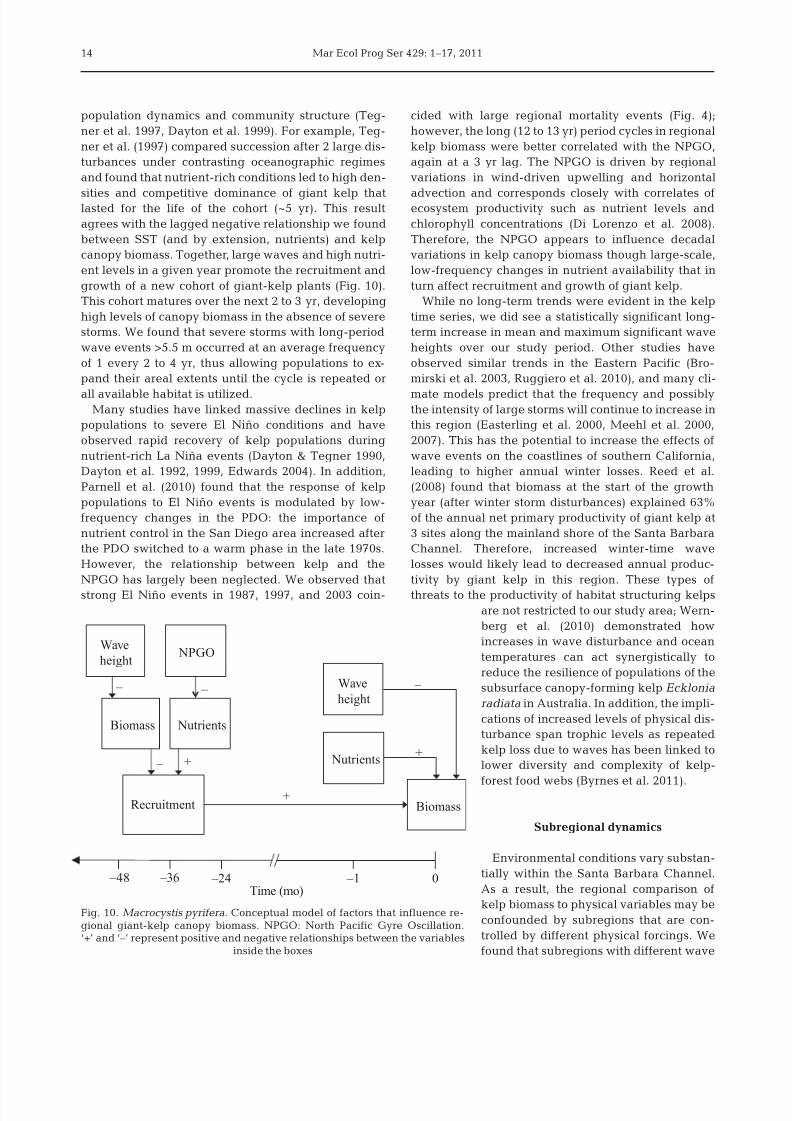
growth of a new cohort of giant-kelp plants (Fig. 10).
This cohort matures over the next 2 to 3 yr, developing
high levels of canopy biomass in the absence of severe
storms. We found that severe storms with long-period
wave events >5.5 m occurred at an average frequency
of 1 every 2 to 4 yr, thus allowing populations to ex-
pand their areal extents until the cycle is repeated or
all available habitat is utilized.Many studies have linked massive declines in kelp
populations to severe El Niño conditions and have
observed rapid recovery of kelp populations during
nutrient-rich La Niña events (Dayton & Tegner 1990,
Dayton et al. 1992, 1999, Edwards 2004). In addition,
Parnell et al. (2010) found that the response of kelp
populations to El Niño events is modulated by low-
frequency changes in the PDO: the importance of
nutrient control in the San Diego area increased after
the PDO switched to a warm phase in the late 1970s.
However, the relationship between kelp and the
NPGO has largely been neglected. We observed that
strong El Niño events in 1987, 1997, and 2003 coin-
cided with large regional mortality events (Fig. 4);
however, the long (12 to 13 yr) period cycles in regional
kelp biomass were better correlated with the NPGO,
again at a 3 yr lag. The NPGO is driven by regional
variations in wind-driven upwelling and horizontal
advection and corresponds closely with correlates ofecosystem productivity such as nutrient levels and
chlorophyll concentrations (Di Lorenzo et al. 2008).
Therefore, the NPGO appears to influence decadal
variations in kelp canopy biomass though large-scale,
low-frequency changes in nutrient availability that in
turn affect recruitment and growth of giant kelp.
While no long-term trends were evident in the kelp
time series, we did see a statistically significant long-
term increase in mean and maximum significant wave
heights over our study period. Other studies have
observed similar trends in the Eastern Pacific (Bro-
mirski et al. 2003, Ruggiero et al. 2010), and many cli-
mate models predict that the frequency and possiblythe intensity of large storms will continue to increase in
this region (Easterling et al. 2000, Meehl et al. 2000,
2007). This has the potential to increase the effects of
wave events on the coastlines of southern California,
leading to higher annual winter losses. Reed et al.
(2008) found that biomass at the start of the growth
year (after winter storm disturbances) explained 63%
of the annual net primary productivity of giant kelp at
3 sites along the mainland shore of the Santa Barbara
Channel. Therefore, increased winter-time wave
losses would likely lead to decreased annual produc-
tivity by giant kelp in this region. These types of
threats to the productivity of habitat structuring kelps
are not restricted to our study area; Wern-
berg et al. (2010) demonstrated how
increases in wave disturbance and ocean
temperatures can act synergistically to
reduce the resilience of populations of the
subsurface canopy-forming kelp Ecklonia
radiata in Australia. In addition, the impli-
cations of increased levels of physical dis-
turbance span trophic levels as repeated
kelp loss due to waves has been linked to
lower diversity and complexity of kelp-
forest food webs (Byrnes et al. 2011).
Subregional dynamics
Environmental conditions vary substan-
tially within the Santa Barbara Channel.
As a result, the regional comparison of
kelp biomass to physical variables may be
confounded by subregions that are con-
trolled by different physical forcings. We
found that subregions with different wave
14
BiomassRecruitment
Wave
height
Nutrients
Wave
height
NutrientsBiomass
–
– ++
–
+
–1 –24 –36 –48 0Time (mo)
NPGO
–
Fig. 10. Macrocystis pyrifera. Conceptual model of factors that influence re-
gional giant-kelp canopy biomass. NPGO: North Pacific Gyre Oscillation.‘+’ and ‘–’ represent positive and negative relationships between the variables
inside the boxes
8/3/2019 Cavanaugh 2011 Environmental Controls of Santa Barbara Kelp
http://slidepdf.com/reader/full/cavanaugh-2011-environmental-controls-of-santa-barbara-kelp 15/17
Cavanaugh et al.: Environmental controls of giant-kelp biomass
exposures responded differently to variations in wave
heights and SST (Table 2). The dynamics of the rela-
tively sheltered mainland coastline south of Point Con-
ception (Subregion D) were significantly negatively
correlated with SST, but not maximum wave height.
Tegner et al. (1996) observed similar behavior in thePoint Loma kelp forest near San Diego: a measure of
canopy density was significantly negatively correlated
with SST but not wave heights. Also, in many years,
minimum canopy biomass levels occurred in late sum-
mer-early fall for Subregion D (Fig. 9). This is generally
a time of relatively low wave energy and low nutrient
levels, suggesting that senescence unrelated to waves
is causing these annual minimums. The large variation
in the timing of annual maximums and minimums for
Subregion D results from variability in the timing of
storms large enough to affect this sheltered region as
well as temporal variability in nutrient conditions each
year.Our results indicate that Point Conception marks a
major biogeographic boundary for the seasonal dy-
namics of giant-kelp forests in California. Changes in
kelp biomass along the exposed coastline north of
Point Conception were well-correlated with wave
height, but not SST as high storm mortalities were
observed each winter. This created a pronounced and
predictable seasonal cycle with lower interannual vari-
ability than the more sheltered subregions to the south
(Fig. 9). The high variation in canopy biomass ob-
served in October and November (e.g. long boxes in
Fig. 9A) reflect variability in the timing of the onset of
the winter storm season. Relatively high nutrient con-
ditions in this subregion likely allowed for consistent
spring and summer recovery each year (Jackson 1987).
This result agrees with those of Donnellan (2004), who
found that seasonal canopy dynamics of exposed cen-
tral Californian kelp beds were highly regular and pre-
dictable. The subregions containing the Santa Barbara
Channel Islands represented a combination of more
complex exposure and nutrient conditions. Seasonality
of kelp biomass in Subregion B was similar to that of
the exposed Subregion A, but Subregion B displayed a
higher variability in the timing of annual minimums
that was likely due to the higher variability of expo-sures contained in this subregion. Subregion B showed
consistent spring recovery each year, probably reflect-
ing the fact that biomass dynamics of this subregion
are rarely limited by nutrients. Like the coastline north
of Point Conception, the south sides of the 2 western-
most Channel Islands are typically bathed in nutrient-
rich water (Otero & Siegel 2004, McPhee-Shaw et al.
2007).
Previous studies have shown fluctuations in kelp
abundance on cycles of 3 to 5 yr and have suggested
that these fluctuations result from seasonal forcings
such as wave disturbance (Dayton et al. 1984, Graham
et al. 1997). Nisbet & Bence (1989) developed a family
of 2-stage kelp population models (juvenile and adults)
that reproduced 3 to 5 yr cycles as well as shorter-
period 1 yr cycles. Their models were based on the
idea that population dynamics are driven by recruit-ment events, which are in turn controlled by tem-
perature, bottom irradiance, and unknown stochastic
factors. Their models predicted that larger seasonal
fluctuations in surface irradiance and adult mortality,
such as those driven by wave disturbance, should lead
to more regular annual recruitment as mortality of
adults each year frees up space and resources (i.e.
light) for new recruits. On a regional scale, we found
that exposed coastlines experienced more regular
annual cycles of winter mortality and spring recovery
than did sheltered regions. Our observation of greater
regularity of the annual cycles in exposed regions is in
contrast to that observed by Graham et al. (1997) incentral California and may reflect differences in the
spatial scales over which kelp was measured in the 2
studies (i.e. m2 in Graham et al. 2007 vs. km2 in the
present study). The dynamics of giant kelp at field-
transect scales do not always reflect dynamics at the
forest or regional scales (Cavanaugh et al. 2010).
The present work represents the most spatially and
temporally comprehensive analysis of the drivers of
giant-kelp biomass to date. We have shown that there
is a large amount of regional heterogeneity in the
response of kelp biomass to different environmental
factors, demonstrating that conclusions drawn from
local studies cannot always be applied to regional
scales. The roles of environmental drivers of kelp bio-
mass also vary in time, making it difficult to predict the
response of this system to future changes in environ-
mental conditions. Continued large-scale and long-
term observations are needed to better our under-
standing of how ecosystems may behave differently in
a future climate.
Acknowledgements. We acknowledge the support of theNASA Biodiversity and Ecological Forecasting Science pro-
gram, NASA’s support of K.C.C. through the Earth SystemScience fellowship program, and the National Science Foun-
dation’s support of the Santa Barbara Coastal Long Term Eco-logical Research (SBC LTER) site. We thank the numerous
SBC LTER divers for collection of data in the field. M. Grahamand 2 anonymous reviewers provided valuable comments on
the manuscript.
LITERATURE CITED
Adams J, Smith M, Gillespie A (1993) Im aging spectroscopy:
interpretation based on spectral mixture analysis. In:Pieters CM, Englert P (eds) Remote geochemical analy-
sis: elemental and mineralogical composition. Cambridge University Press, New York, NY, p 145–166
15

8/3/2019 Cavanaugh 2011 Environmental Controls of Santa Barbara Kelp
http://slidepdf.com/reader/full/cavanaugh-2011-environmental-controls-of-santa-barbara-kelp 16/17
Mar Ecol Prog Ser 429: 1–17, 2011
Adams P, Inman D, Graham N (2008) Southern California
deep-water wave climate: characterization and applica-tion to coastal processes. J Coast Res 24:1022–1035
Baardseth E (1970) A square-scanning, two stage samplingmethod of estimating seaweed quantities. Rep Norw Inst
Seaweed Res 33:1–41
Baugh W, Groeneveld D (2008) Empirical proof of the empiri-cal line. Int J Remote Sens 29:665–672Behrenfeld M, O’Malley R, Siegel D, McClain C and others
(2006) Climate-driven trends in contemporary ocean pro-ductivity. Nature 444:752–755
Berk A, Bernstein L, Anderson G, Acharya P, Robertson D,ChetwyndJ, Adler-GoldenS (1998) MODTRAN cloud and
multiple scattering upgrades with application to AVIRIS.
Remote Sens Environ 65: 367–375Britton-Simmons K, Eckman JE, Duggins DO (2008) Effect of
tidal currents and tidal stage on estimates of bed size in thekelp Nereocystis luetkeana. Mar Ecol Prog Ser 355:95–105
Bromirski P, Flick R, Cayan D (2003) Storminess variabilityalong the California coast: 1858–2000. J Clim 16:982–993
Byrnes JE, Reed DC, Cardinale BJ, Cavanaugh KC, HolbrookSJ, Schmitt RJ (2011) Climate-driven increases in storm
frequency simplify kelp forest food webs. Glob ChangeBiol (in press) doi:10.1111/j.1365-2486.2011.02409.x
Cavanaugh KC, Siegel DA, Kinlan BP, Reed DC (2010) Scal-ing giant kelp field measurements to regional scales using
satellite observations. Mar Ecol Prog Ser 403:13–27
Clendenning KA, Sargent MC (1971) Photosynthesis andgeneral development in Macrocystis . Nova Hedwigia 32:
169–190Dayton P, Tegner M (1990) Bottoms beneath troubled waters:
benthic impacts of the 1982–1984 El Niño in the tempera-ture zone. Elsevier Oceanogr Ser 52:433–472
Dayton P, Currie V, Gerrodette T, Keller B, Rosenthal R, VanTresca D (1984) Patch dynamics and stability of some
California kelp communities. Ecol Monogr 54:253–289Dayton P, Tegner M, Parnell P, Edwards P (1992) Temporal
and spatial patterns of disturbance and recovery in a kelpforest community. Ecol Monogr 62:421–445
Dayton P, Tegner M, Edwards P, Riser K (1999) Temporal andspatial scales of kelp demography: the role of oceano-
graphic climate. Ecol Monogr 69:219–250
Dennison P, Roberts D (2003a) The effects of vegetation phe-nology on endmember selection and species mapping in
southern California chaparral. Remote Sens Environ 87:295–309
Dennison P, Roberts D (2003b) Endmember selection for mul-tiple endmember spectral mixture analysis using end-
member average RMSE. Remote Sens Environ 87:123–135Deysher L (1993) Evaluation of remote sensing techniques for
monitoring giant kelp populations. Hydrobiologia 260-261:307–312
Deysher L, Dean T (1986) In situ recruitment of sporophytes of
the giant kelp Macrocystis pyrifera (L.) C.A. Agardh:effects of physical factors. J Exp Mar Biol Ecol 103:41–63
Di Lorenzo E, Schneider N, Cobb K, Franks P and others(2008) North Pacific Gyre Oscillation links ocean climate
and ecosystem change. Geophys Res Lett 35:L08607 doi:10.1029/2007GL032838
Doney S, Fabry V, Feely R, Kleypas J (2009) Ocean acidifica-tion: the other CO2 problem. Annu Rev Mar Sci 1:169–192
Donnellan M (2004) Spatial and temporal variability of kelpforest canopies in central California. MS thesis, San Jose
State University, San Jose, CAEasterling D, Meehl G, Parmesan C, Changnon S, Karl T,
Mearns L (2000) Climate extremes: observations, model-ing, and impacts. Science 289:2068–2074
Edwards MS (2004) Estimating scale-dependency in distur-
bance impacts: El Niños and giant kelp forests in thenortheast Pacific. Oecologia 138:436–447
FramJ, Stewart H, Brzezinski M, Gaylord B, Reed D, WilliamsS, MacIntyre S (2008) Physical pathways and utilization
of nitrate supply to the giant kelp, Macrocystis pyrifera.
Limnol Oceanogr 53:1589–1603Furby S, Campbell N (2001) Calibrating images from differentdates to ‘like-value’ digital counts. Remote Sens Environ
77:186–196Graham MH, Harrold C, Lisin S, Light K, Watanabe JM,
Foster MS (1997) Population dynamics of giant kelp
Macrocystis pyrifera along a wave exposure gradient. Mar
Ecol Prog Ser 148:269–279
Graham M, Vasquez J, Buschmann A (2007) Global ecologyof the giant kelp Macrocystis : from ecotypes to ecosys-
tems. Oceanogr Mar Biol Annu Rev 45:39–88Harley C, Randall Hughes A, Hultgren K, Miner B and others
(2006) The impacts of climate change in coastal marinesystems. Ecol Lett 9:228–241
Harms S, Winant C (1998) Characteristic patterns of the circu-lation in the Santa Barbara Channel. J Geophys Res 103:
3041–3065Hickey B (1979) The California current system— hypotheses
and facts. Prog Oceanogr 8:191–279Hoegh-Guldberg O, Bruno J (2010) The impact of climate
change on the world’s marine ecosystems. Science 328:1523–1528
Huth R (1996) An intercomparison of computer-assisted circu-
lation classification methods. Int J Climatol 16:893–922Jackson G (1987) Modelling the growth and harvest yield of
the giant kelp Macrocystis pyrifera. Mar Biol 95:611–624Jensen JR, Estes JE, Tinney L (1980) Remote sensing tech-
niques for kelp surveys. Photogramm Eng Remote Sensing46:743–755
Lee D, Storey J, Choate M, Hayes R (2004) Four years ofLandsat-7 on-orbit geometric calibration and performance.
IEEE Trans Geosci Remote Sens 42:2786–2795Legendre P, Legendre L (1998) Numerical ecology, 2nd
English edn. Elsevier Science, AmsterdamLi L, Ustin S, Lay M (2005) Application of multiple end-
member spectral mixture analysis (MESMA) to AVIRIS
imagery for coastal salt marsh mapping: a case study inChina Camp, CA, USA. Int J Remote Sens 26:5193–5207
Mantua N, Hare S, Zhang Y, Wallace J, Francis R (1997) APacific interdecadal climate oscillation with impacts on
salmon production. Bull Am Meteorol Soc 78:1069–1079Markham B, Storey J, Williams D, Irons J (2004) Landsat sen-
sor performance: history and current status. IEEE TransGeosci Remote Sens 42:2691–2694
McPhee-Shaw EE, Siegel DA, Washburn L, Brzezinski MA,Jones JL, Leydecker A, Melack J (2007) Mechanisms
for nutrient delivery to the inner shelf: observations
from the Santa Barbara Channel. Limnol Oceanogr 52:1748–1766
Meehl G, Zwiers F, Evans J, Knutson T, Mearns L, Whetton P(2000) Trends in extreme weather and climate events:
issues related to modeling extremes in projections offuture climate change. Bull Am Meteorol Soc 81:427–436
Meehl G, Stocker T, Collins W, Friedlingstein P and others(2007) Global climate projections. In: Qin D, Manning M,
Chen Z, Marquis M, Averyt K, Tignor M, Miller HL (eds)Climate change 2007: the physical science basis. Contri-
bution of Working Group I to the Fourth AssessmentReport of the Intergovernmental Panel on Climate Change.
Cambridge University Press, New York, NY, p 747–845Nisbet R, Bence J (1989) Alternative dynamic regimes for
16
®
®
®®
®
®
®
®
®
®
®
®
®
®
®
®
®
®
®®
®®
®
®
®
®®
®
®
®®
®
®
®
®
®
®
®
®
®
8/3/2019 Cavanaugh 2011 Environmental Controls of Santa Barbara Kelp
http://slidepdf.com/reader/full/cavanaugh-2011-environmental-controls-of-santa-barbara-kelp 17/17
Cavanaugh et al.: Environmental controls of giant-kelp biomass 17
canopy-forming kelp: a variant on density-vague popula-
tion regulation. Am Nat 134:377–408North WJ, Zimmerman RC (1984) Influences of macronutri-
ents and water temperatures on summertime survival ofMacrocystis canopies. Hydrobiologia 116-117:419–424
O’Reilly W, Guza R (1993) A comparison of two spectral wave
models in the Southern California Bight. Coast Eng 19:263–282Okin G, Roberts D, Murray B, Okin W (2001) Practical limits
on hyperspectral vegetation discrimination in arid andsemiarid environments. Remote Sens Environ 77:212–225
Otero M, Siegel D (2004) Spatial and temporal characteristicsof sediment plumes and phytoplankton blooms in the
Santa Barbara Channel. Deep-Sea Res II 51:1129–1149
Parnell PE, Miller EF, Lennert-Cody CE, Dayton PK, CarterML, Stebbins TD (2010) The response of giant kelp (Macro -
cystis pyrifera) in southern California to low-frequency cli-mate forcing. Limnol Oceanogr 55:2686–2702
Peterson W, Schwing F (2003) A new climate regime in North-east Pacific ecosystems. Geophys Res Lett 30:1896 doi:
10.1029/2003GL017528Przeslawski R, Ahyong S, Byrne M, Woerheide G, Hutchings
P (2008) Beyond corals and fish: the effects of climatechange on noncoral benthic invertebrates of tropical reefs.
Glob Change Biol 14:2773–2795Rassweiler A, Arkema K, Reed D, Zimmerman R, Brzezinski
M (2008) Net primary production, growth, and standing
crop of Macrocystis pyrifera in southern California. Eco-logy 89:2068
Reed D, Foster M (1984) The effects of canopy shadings onalgal recruitment and growth in a giant kelp forest. Eco-
logy 65:937–948Reed D, Ebeling A, Anderson T, Anghera M (1996) Differen-
tial reproductive responses to fluctuating resources in twoseaweeds with different reproductive strategies. Ecology
77:300–316Reed D, Rassweiler A, Arkema K (2008) Biomass rather than
growth rate determines variation in net primary produc-tion by giant kelp. Ecology 89:2493–2505
Roberts D, Gardner M, Church R, Ustin S, Scheer G, Green R(1998) Mapping chaparral in the Santa Monica Mountains
using multiple endmember spectral mixture models.
Remote Sens Environ 65:267–279Rosenzweig C, Karoly D, Vicarelli M, Neofotis P and others
(2008) Attributing physical and biological impacts toanthropogenic climate change. Nature 453:353–357
Ruggiero P, Komar P, Allan J (2010) Increasing wave heights
and extreme value projections: the wave climate of theUS Pacific Northwest. Coast Eng 57:539–552Seymour R (1998) Effects of El Niños on the west coast wave
climate. Shore Beach 66:3–6Smith CA, Sardeshmukh PD (2000) The effect of ENSO on the
intraseasonal variance of surface temperatures in winter.Int J Climatol 20:1543–1557
Stekoll MS, Deysher LE, Hess M (2006) A remote sensing
approach to estimating harvestable kelp biomass. J ApplPhycol 18:323–334
Tegner MJ, Dayton PK, Edwards PB, Riser KL (1996) Is thereevidence for long-term climatic change in southern Cali-
fornia kelp forests? Calif Coop Ocean Fish Invest Rep37:111–126. Available at: www.calcofi.org/publications/
ccreports/118-vol37-1996.htmlTegner MJ, Dayton PK, Edwards PB, Riser KL (1997) Large-
scale, low-frequency oceanographic effects on kelp forest succession: a tale of two cohorts. Mar Ecol Prog Ser 146:
117–134Utter B, Denny M (1996) Wave-induced forces on the giant
kelp Macrocystis pyrifera (Agardh): field test of a compu-
tational model. J Exp Biol 199:2645Wernberg T, Thomsen MS, Tuya F, Kendrick GA, Staehr PA,
Toohey BD (2010) Decreasing resilience of kelp bedsalong a latitudinal temperature gradient: potential impli-
cations for a warmer future. Ecol Lett 13:685–694Youngentob K, Roberts D, Held A, Dennison P, Jia X, Linden-
mayer D (2011) Mapping two Eucalyptus subgenera usingmultiple endmember spectral mixture analysis and contin-
uum-removed imaging spectrometry data. Remote SensEnviron 115:1115–1128
Zimmerman RC, Kremer JN (1986) In situ growth and chemi-cal composition of the giant kelp, Macrocystis pyrifera:
response to temporal changes in ambient nutrient avail-
ability. Mar Ecol Prog Ser 27:277–285
Editorial responsibility: Lisandro Benedetti-Cecchi,
Pisa, Italy
Submitted: December 13, 2010; Accepted: March 21, 2011
Proofs received from author(s): May 5, 2011
®
®
®
®
®®
®
®
®®
®
®®
®
®
®
®
®®
®
®