CATS regression – a model-based approach to study-

ing trait-based community assembly

David I. Warton1, Bill Shipley2 and Trevor Hastie3

1School of Mathematics and Statistics and Evolution & Ecology Research Centre, The University of

New South Wales, NSW 2052, Australia2Departement de Biologie, Universite de Sherbrooke, Sherbrooke, J1K 2R1, Canada3Department of Statistics, Stanford University, Stanford, CA 94305, The United States of America

Running Header - GLMs for trait-based community assembly

Word count: 6965 words

Summary

1. Shipley et al. (2006) proposed a maximum entropy approach to studying

how species relative abundance is mediated by their traits, “community as-

sembly via trait selection” (CATS).

2. In this paper we build on recent equivalences between the maximum en-

tropy formalism and Poisson regression to show that CATS is equivalent to a

generalised linear model for abundance, with species traits as predictor vari-

ables.

3. Main advantages gained by access to the machinery of generalised linear

models can be summarised as advantages in interpretation, model-checking,

extensions and inference.

4. A more difficult issue however is the development of valid methods of infer-

ence for single-site data, as species correlation in abundance is not accounted

for in CATS (whether specified as a regression or via maximum entropy). This

issue can be circumvented for multi-site data using design-based inference.

5. These points are illustrated by example – our plant abundances were found

to violate the implicit Poisson assumption of CATS, but a negative binomial

regression had much-improved fit, and our model was extended to multi-site

data in order to directly model the environment-trait interaction. Keywords:

community composition, community-level models, fourth corner model, gener-

alised linear models, maximum entropy, Poisson regression

1

Much of the recent multivariate literature in ecology has focussed on describing the re-

sponse to environmental conditions of different species (Wang et al., 2012) or of aggregate

quantities computed from species, such as diversity measures (Anderson et al., 2011) or

pair-wise dissimilarities (Anderson, 2001; Ferrier & Guisan, 2006). But a key challenge

is describing not just how species differ, but why, a question which can only be answered

by looking at the traits of different species (McGill et al., 2006) and how traits mediate

differences in abundance across species and environments.

Community assembly by trait selection (Shipley et al., 2006, “CATS”) is a means of

studying how traits drive differences in relative abundance of different species at a site.

The method was originally developed for analysis of data from a single site, where we

have recorded a quantitative measure of relative abundance of each species (e.g. count,

biomass), and a set of traits of each species (e.g. plant height, leaf mass per area) that

might be considered to be drivers of relative abundance. More recently the method has

been used in a multi-site context via a two-stage approach – analysing trait data sep-

arately at each site, then analysing summary statistics across sites to relate results to

environmental variables (Sonnier et al., 2012). In this paper we will extend the function-

ality of CATS in various ways, including allowing multi-site analysis to be approached

directly within a single model. This is achieved by exploiting an equivalence between

maximum entropy and Poisson regression.

Equivalences between maximum entropy methods and maximum likelihood have a long

history. Maximum entropy was related to maximum likelihood for exponential families

by Kullback (1959) and for contingency table analysis (Good, 1963). More recently, max-

imum entropy was linked to maximum likelihood of a Gibbs distribution (Della Pietra

et al., 1997) and the multinomial distribution (Shipley et al., 2012, Appendix A). In the

species distribution modelling literature, an equivalence result recently connected maxi-

mum entropy methods to generalised linear models – it has been shown in the context of

presence-only analysis that estimating probabilities of species occurrence via a maximum

entropy approach (Phillips et al., 2006, “MAXENT”) is equivalent to Poisson regression

and Poisson point process regression (Renner & Warton, 2013; Fithian & Hastie, in press).

This equivalence made possible a number of extensions to MAXENT – including the use

of diagnostic tools standard in the regression literature for model-checking, extensions of

the model when assumptions are not satisfied, and inference tools to account for uncer-

tainty in fitted models. In this paper, it will be shown that a similar equivalence result

extends to CATS models and offers some of these same advantages.

2

1 Main result

Consider observations of the abundance of S different species in a site, y = (y1, . . . , yS),

with total abundance n =∑S

i=1 yi. For each species, K traits are measured, and for

the ith species these are stored in xi = (xi1, . . . , xiK). Our goal is to study how relative

abundances (yin

) across species are associated with traits (xi).

Sometimes we also have estimates of qi, the relative abundance of each species in the meta-

community. Shipley (2010) referred to these as “prior” abundances. When available, these

should usually be incorporated into the analysis also, in order to account for the fact that

the relative abundance of a species at a site is a function of its abundance in the broader

metacommunity as well as being a function of the species’ suitability to the site. This is

related to the concept of community assembly via environmental filtering (Shipley, 2010).

1.1 CATS specification

In CATS we wish to predict the relative abundance of each species (pi) to maximise

relative entropy or Kullback-Leibler divergence:

−S∑i=1

pi ln

(piqi

)(1)

subject to the constraints:

S∑i=1

pi = 1,S∑i=1

pixij =1

n

S∑i=1

yixij (2)

The observed relative abundances enter into analyses through the second constraint in

equation 2. The solution can be found using the Lagrangian method, and it has the form:

pi = qieλ−1+x′

iβ

or in log-linear form:

ln pi = ln qi + λ− 1 + x′iβ

The key coefficient of interest is β, a vector of K “selection coefficients”, summarising the

strength of association between each of the traits and relative abundance. The parameter

λ controls the predicted abundance of each species such that the pi sum to one.

When no information about metacommunity abundance is available, the qi are uniform,

and Equation (1) reduces to the entropy function (Shannon & Weaver, 1949), in which

case CATS can be understood as maximum entropy estimation along the lines of Phillips

et al. (2006).

3

1.2 Equivalence with Poisson regression

Our key result is as follows:

CATS is mathematically equivalent to Poisson regression of the yi against xi,

using qi as an offset.

That is, CATS can be understood as fitting a log-linear model for the mean abundance

of each species (µi):

lnµi = ln qi + β0 + x′iβ

where parameters β0 and β are estimated to maximise the Poisson likelihood:

`(β0,β; y) =S∑i=1

yi lnµi − µi

The regression slope coefficients β are exactly the selection coefficients as in Shipley et al.

(2006), and the intercept has been shifted by a constant β0 = λ0 + 1 + lnn.

The proof of this result is relatively straightforward and can be found at the end of

this article. The mathematics of the proof are very similar to that found in Renner

& Warton (2013), where it was similarly shown that maximum entropy estimation of

presence-only data can be understood as Poisson regression. The essential differences here

are: the response variable is now abundance rather than presences of a species in grid

cells (although this has no implications for the mathematics); CATS maximises relative

entropy of predicted relative abundance pi as compared to a prior qi (which resulted in

the addition of an offset, log(qi), not found in Renner & Warton, 2013).

Thus CATS can be implemented via generalised linear modelling (GLM) functions avail-

able on most statistics software, for example, on R:

glm(rel~trait+offset(log(meta)),family="poisson")

where for each species the relative abundance is stored in rel, trait measurements in

trait, and “prior” relative abundance from the metacommunity in meta. We will refer

to this in the following as an example of “CATS regression”.

2 Implications

The above equivalence result has a number of implications, but the most important can

be summarised as relating to interpretation, model-checking, extensions and inference.

4

2.1 Interpretation

It is anticipated that because most readers will be familiar with regression techniques,

many will find it helpful to think of CATS as a regression of abundances of different

species at a site against their species traits.

Further, thinking of CATS as a regression problem helps clarify some issues previously

raised in the literature. In particular, Roxburgh & Mokany (2007) argued that there is

circularity in CATS as proposed in Shipley et al. (2006), due to use of observed abundances

both to fit the model and to compute an R2 goodness-of-fit statistic. Shipley et al. (2007)

responded that the circularity is no greater than that typically experienced in regression

problems (and that it can be taken into account when making statistical inferences).

We have verified this by showing that CATS is in fact a type of regression. Further,

alternative measures of R2 for generalised linear models have been suggested (Cameron &

Windmeijer, 1997; Nakagawa & Schielzeth, 2012) which could be considered as alternatives

to the proposal in Shipley et al. (2006).

Another aspect where thinking of CATS as a regression may assist interpretation is in

understanding the role of the prior qi. The term “prior” is suggestive of Bayesian priors

and the incorporation of prior information, but in a regression context, qi actually has

the role of an offset term. An offset is a variable included in the model that has a known

slope coefficient, usually, a variable known to have a proportionate effect on the response.

Offsets are typically used to account for varying sampling effort across site, e.g. if the

sampling unit is twice as large at a site then our initial expectation is that the abundance

will be twice as large also. Meta-community relative abundance (qi) can be understood

as an offset for similar reasons – all else being equal, a species which is twice as abundant

in the metacommunity is expected to be twice as abundant in the site.

2.2 Model-checking

Because CATS is mathematically equivalent to Poisson regression, arguably, it is subject

to Poisson regression assumptions. Poisson regression assumptions are: (1) observations

are independent (conditional on trait values); (2) abundances are Poisson in distribution;

(3) mean abundance has a log-linear relationship with traits.

Assumption (1) is potentially problematic, as it would be violated by species interactions

that are not explained by traits alone, which has implications for inference, discussed

5

later.

Assumptions (2-3) can be checked using standard diagnostic tools. While not widely used

in ecology and evolution, Dunn-Smyth residuals (Dunn & Smyth, 1996) are especially

useful for this purpose, as they are standard normal in distribution for any parametric

model, whenever the model is correct, and thus are not a function of any explanatory

variables. They can be computed using the residuals.manyglm function in the mvabund

package (Wang et al., 2012), which also uses Dunn-Smyth residuals by default in residual

plots. Dunn-Smyth residual plots provide a helpful visual tool for assessment of the extent

of violations of distributional assumptions, in the same way that ordinary residuals are

often used to diagnose least squares regression. Violation of the mean-variance assump-

tion is characterised by a fan shape on residual vs fits plots, violation of log-linearity is

often expressed via a U -shape on a residual vs fits plot, and systematic departures from

a straight line of slope one on a normal quantile plot can mean violation of either of

these assumptions (but strong non-normality is suggestive of a violation of distributional

assumptions).

2.3 Extensions

An especially exciting prospect is the extension of CATS to other contexts via the regres-

sion framework, e.g. to other data types, multi-site data, to incorporate uncertainty.

Often the Poisson assumption is not reasonable for abundance data. Counts are often

overdispersed compared to the Poisson, in which case negative binomial regression might

be a useful alternative (O’Hara & Kotze, 2010). Abundance might be measured as biomass

or percent cover rather than as a count, in which case the Tweedie distribution (as in

Dunstan et al., 2013) should be considered, given that it is scale invariant but with a

probability mass at zero, and its mean-variance assumption follows Taylor’s power law

(Taylor, 1961). Abundance might be measured on an ordinal scale, in which case, models

developed specially for an ordinal response, such as the proportional odds model (Yee,

2010), are suitable. None of these models is mathematically equivalent to CATS, however,

they can each be argued to have the same goal as CATS but instead use a model which

is better suited to the distributional properties of the abundance data at hand.

While CATS was originally proposed for single site data, extensions to the multi-site

context are quite natural in a regression context. Let yij be the abundance of species i at

site j, and let zj be a vector of environmental variables describing site j. We can fit the

6

model:

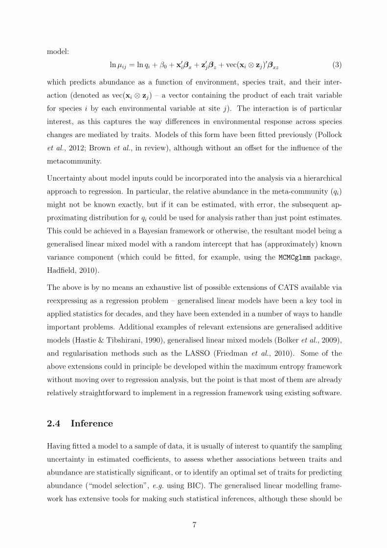
lnµij = ln qi + β0 + x′iβx + z′jβz + vec(xi ⊗ zj)′βxz (3)

which predicts abundance as a function of environment, species trait, and their inter-

action (denoted as vec(xi ⊗ zj) – a vector containing the product of each trait variable

for species i by each environmental variable at site j). The interaction is of particular

interest, as this captures the way differences in environmental response across species

changes are mediated by traits. Models of this form have been fitted previously (Pollock

et al., 2012; Brown et al., in review), although without an offset for the influence of the

metacommunity.

Uncertainty about model inputs could be incorporated into the analysis via a hierarchical

approach to regression. In particular, the relative abundance in the meta-community (qi)

might not be known exactly, but if it can be estimated, with error, the subsequent ap-

proximating distribution for qi could be used for analysis rather than just point estimates.

This could be achieved in a Bayesian framework or otherwise, the resultant model being a

generalised linear mixed model with a random intercept that has (approximately) known

variance component (which could be fitted, for example, using the MCMCglmm package,

Hadfield, 2010).

The above is by no means an exhaustive list of possible extensions of CATS available via

reexpressing as a regression problem – generalised linear models have been a key tool in

applied statistics for decades, and they have been extended in a number of ways to handle

important problems. Additional examples of relevant extensions are generalised additive

models (Hastie & Tibshirani, 1990), generalised linear mixed models (Bolker et al., 2009),

and regularisation methods such as the LASSO (Friedman et al., 2010). Some of the

above extensions could in principle be developed within the maximum entropy framework

without moving over to regression analysis, but the point is that most of them are already

relatively straightforward to implement in a regression framework using existing software.

2.4 Inference

Having fitted a model to a sample of data, it is usually of interest to quantify the sampling

uncertainty in estimated coefficients, to assess whether associations between traits and

abundance are statistically significant, or to identify an optimal set of traits for predicting

abundance (“model selection”, e.g. using BIC). The generalised linear modelling frame-

work has extensive tools for making such statistical inferences, although these should be

7

used with care, because of problems with the independence assumption.

Recall that assumption (1) of Poisson regression was that observations are independent

across species. In ordinary regression problems the independence assumption is often

reasonable by design – for example, by randomly selecting study sites from a population of

potential sites, one can argue that responses are independent. But in studies of community

structure this is not true across species – typically, one records the abundance of all species

at a site, rather than a small sample of them. Further, species interactions are often

expected to occur, due to competition, predation, or a host of other causes (Wisz et al.,

2013). Under these conditions, violations of the independence assumption are arguably

the norm rather than the exception.

Violations of the independence assumption do not invalidate the estimation procedure,

but they do invalidate standard methods of inference under the GLM framework. There

is no simple solution to this problem in the single-site case – to make valid inferences,

one would need to know a priori the form of dependence, parameterised in a simple

enough way that it could be estimated from data at a single site. Shipley et al. (2007)

suggested permutation tests, where one permutes trait values across species, as a way

to address the problem, but that assumes trait values (or equivalently, abundances) are

exchangeable across species, an assumption that is closely related to the independence

assumption across species which was problematic in the first place. Unfortunately, for

data from a single site, there seems little alternative to using standard GLM software

to make approximate inferences about parameter uncertainty, or permutation tests as in

Shipley (2010) for approximate hypothesis tests.

In multi-site analyses, however, there is the potential to use design-based approaches to

inference (Manly, 2007), if the sites have been sampled in such a way that independence

across sites can reasonably be assumed. Estimates of parameter uncertainty could be

obtained by bootstrapping sites, and tests of environment-trait associations could be ob-

tained by resampling all observations from a site jointly, in an analogous fashion to what

is currently done in multivariate analysis in ecology (Anderson, 2001; Wang et al., 2012),

in order to ensure inferences are valid despite potential violations of the assumption of

independence across species. In the context of generalised linear modelling, suitable re-

sampling approaches include case resampling (Davison & Hinkley, 1997) or more recently

the PIT-trap (Warton & Wang, in review), both of which are available in the mvabund

package (Wang et al., 2012).

8

2.5 CATS regression when species abundances are not observed

CATS as originally specified does not require knowledge of the abundance of each species

(yi). Instead, the only abundance information that is required for model-fitting is the

community-aggregated traits, 1n

∑Si=1 yixik = x·k. In fact, software for fitting CATS mod-

els – the maxent function in the FD package (Laliberte & Shipley, 2011) – has been struc-

tured such that it can take the community-aggregated values x·k as input rather than

the abundances yi. This situation might be especially desirable if one wishes to estimate

community-aggregated trait means without measuring abundance of each species (for ex-

ample, using some empirical relationship between community-aggregated trait means and

environmental variables).

Strictly speaking, only community-aggregated traits are required to fit a Poisson CATS

regression also, but in practice GLM software does not automatically cater for this option.

The community-aggregated traits x·k are examples of what is known as sufficient statistics

(Gill, 2001) – x·k is sufficient for βk, and a Poisson regression can be fitted directly from

the sufficient statistics, without knowledge of the abundance values for each species at a

site. However most GLM software is not designed to take sufficient statistics as input. In

supplementary material we demonstrate that when using R software, analysis via sufficient

statistics is possible but more indirect via glm than via the maxent function.

The community aggregated traits are sufficient statistics only in the special case of Pois-

son regression. If data were overdispersed relative to the Poisson, such that a negative

binomial regression would be desired, the x·k would no longer be sufficient – essentially,

because more abundant species would need to be down-weighted when averaging trait

values, to account for overdispersion. Thus some of the gains made by moving away from

Poisson models come at a cost to interpretability – the motivating equation for CATS

(Equation 2), that predicted community-aggregated trait values should equal observed

values, may no longer apply.

3 Example

To illustrate some potential advantages afforded by the regression framework we revisit an

analysis of the effects of land use on plant communities in southern France (Sonnier et al.,

2012). Counts of the number of individuals were recorded for each plant species in each of

32 plots, each belonging to one of four treatments, specified according to a combination

9

of grazing history and soil type. Twelve traits were measured on each of the 68 most

abundant species, related to different aspects of leaf properties, size, and phenology. Our

analyses make use of the ten trait variables we had access to (all traits from Sonnier et al.,

2012 but plant lifespan and date of seed maturation). No metacommunity abundance data

(qi) were available so we did not include an offset in any analyses.

It is of interest to understand which traits tend to be related to abundance, and in

particular, to differences in abundance across treatments. For illustratory purposes, data

will be analysed from a single example plot, then from all sites simultaneously.

The R program (R Core Team, 2013) was used for all analyses, using the maxent function

from the FD package (Laliberte & Shipley, 2011) for CATS analysis via maximum entropy,

the glm function from the base package for Poisson regression, and the manyglm function

from the mvabund package (Wang et al., 2012) for negative binomial regression. All leaf

and size variables were log10-transformed prior to analysis. Example R code is included

in supplementary material.

3.1 Single-site analysis

For purposes of illustration we started by re-analysing abundance data from the first listed

site in the dataset, sampled from fertilised pasture on limestone bedrock, using just two

trait variables – leaf dry matter content (LDMC) and leaf carbon content (LCC). At this

site, n = 167 individuals from S = 14 different species were recorded as present.

A CATS analysis via maximum entropy returned slope coefficients that were similar but

not quite identical to Poisson regression results (Table 1), once the convergence tolerance

was increased to a sufficiently high value (the model did not seem to have converged

under default settings). On further decreasing the tolerance to 10−16, the maxent function

returned results that were equal to default output from a Poisson regression obtained via

the glm function to eight decimal places. As expected, the intercepts did not agree,

largely because maximum entropy modelled relative abundance (yi/n), whereas Poisson

regression modelled absolute abundance (yi). Computation time was noticeably longer for

the maxent function than when using the glm function. At a tolerance of 10−16, maxent

took 14 seconds on a laptop with a 2.8GHz processor, whereas glm took less than one

hundredth of a second.

Model checks (Figure 1, left column) suggested data were overdispersed compared to a

Poisson distribution, with Dunn-Smyth residuals “fanning out” at larger predicted values

10

to a much broader range than would be plausible for a standard normal random variable

(with five of the 14 residuals having an absolute value greater than 4, when we should

expect none to exceed 4). Fitting a negative binomial model instead produced much more

favourable residual plots (Figure 1, right column) and a substantially smaller BIC value

(Table 1), suggesting the negative binomial was a much improved model for the data.

Of particular interest from the fitted model is the size and direction of the slope param-

eters, and how large they are relative to sampling uncertainty. The coefficient of leaf

carbon concentration from the negative binomial regression was clearly not significantly

different from zero, whereas there is perhaps some evidence of an increasing relation-

ship between leaf dry matter content and abundance (with an approximate Z-score of

7.252/2.736 = 2.65, but note this is only approximate so should be interpreted conser-

vatively). As compared to the original Poisson model, note that the negative binomial

regression slope parameter for LCC was much flatter and of a different sign, and all

standard errors increased three-fold or more, due to the additional overdispersion now

accounted for in the model. While negative binomial regression suggested a weak, non-

significant positive association between LCC and abundance, Poisson analyses suggested

a marginally significant negative association. Clearly, failing to take into account overdis-

persion can have considerable impacts on the fitted model and its interpretation.

3.2 Multi-site analysis

An interesting extension of CATS regression is to simultaneously analyse plant abundances

from all 32 sites in order to study how traits mediate inter-specific differences in response

to treatment (grazing history and soil type). We fitted the mean model specified in

equation 3, using a negative binomial distribution. We also considered a Poisson, but as

before, data were strongly overdispersed – see supplementary material for details.

Of particular interest are interaction terms between treatment and trait variables – a

significant interaction suggests that there are differences in mean abundance at different

sites that are mediated by traits. We would like to use resampling to enable valid inference

despite potential failure of correlation assumptions, and residual resampling (resampling

by site) is a natural tool which can be used to this end (Manly, 2007). A difficulty comes in

defining residuals for non-normal data, but Warton & Wang (in review) have addressed

this using probability integral transform (PIT-) residuals (along the lines of Dunn &

Smyth, 1996). They refer to the subsequent resampling algorithm as the PIT-trap (a

11

bootstrap using PIT-residuals).

The log-likelihood ratio statistic testing for a treatment× trait interaction is 166.6, which

was significantly large under PIT-trap resampling of residuals across sites (P ≤ 0.001).

Thus we conclude that across these 32 sites and ten trait variables, there is a significant

interaction between (some of the) traits and treatment.

Having established that there is an interaction, the next step is to understand which traits

are most strongly associated with a treatment response. One way to approach this prob-

lem is to estimate standardised interaction coefficients – traits with interaction coefficients

which are larger in magnitude have greater importance (Figure 2). Note that these coeffi-

cients estimate conditional effects, i.e. after accounting for the effects of all other terms in

the model. For example, results suggest that plants with high leaf phosphorous content

(large LPC), when keeping other traits constant, have higher abundance at fertilised and

heavily grazed sites, but lower abundance at sites with nutrient-poor dolomite soils.

A number of alternative approaches to estimating relative importance of traits are avail-

able, many of which can be readily implemented using standard software – including a

leave-one-out approach, or stepwise selection of traits (the drop1 and step functions on

R, respectively), both illustrated in supplementary material.

4 Discussion

Community assembly by trait selection (Shipley, 2010, “CATS”) is a tool for studying

how traits drive interspecific differences in abundance at a site, and by reexpressing CATS

in a regression framework, we have extended its functionality to handle a broader range

of data types and questions. CATS regression can be applied using any measure of

abundance as the response (provided that the model for the response variable is adapted

to the data at hand). Further, CATS regression can be readily extended to handle data

from multiple sites simultaneously, and thus get at the important question of how traits

mediate differences in environmental response across species.

Reanalysis of the plant abundance data from Sonnier et al. (2012) highlighted some of the

potential advantages of reexpressing CATS in a regression framework. Comparing results

to what was previously available in the maximum entropy CATS framework, it is evident

that regression modelling enables: model-checking (Figure 1), with in this case clear ev-

idence against the Poisson assumption which underpins maximum entropy; extensions,

12

in this case involving use of negative binomial regression to account for overdispersion

compared to the Poisson, and multi-site analyses to identify the traits important to com-

munity assembly which interact with environmental conditions (Figure 2); and inference,

with standard errors for assessing uncertainty in parameter estimates and BIC for model

selection (Table 1), and design-based inference in the multi-site analyses. Note however,

as previously, that model-based inference tools (as used in Table 1) require the assump-

tion of independence of observations, and given the potential violation of this assumption

by species interactions, inference from this model should be treated as approximate.

In the single-site analysis, computation time was thousands of times faster for GLM

software than when using maximum entropy software, to achieve a given level of accuracy.

While maximum entropy software still completed analyses in a quarter of a minute, in

other contexts differences in computation time may be practically important (e.g. when

repeating analyses across many sites or trait combinations, when analysing larger datasets,

or when permutation testing). Similarly substantial improvements in computation time

were noticed when moving from MAXENT to GLM software for presence-only analysis

(Renner & Warton, 2013), as well as occasional incorrect solutions in MAXENT, seen here

also when using default settings. Perhaps there is potential to improve maximum entropy

algorithms, and their implementation, by borrowing ideas from the GLM literature.

Strictly speaking, the maximum entropy formalism does not involve an explicit Poisson

assumption – the Poisson assumption only arises “by association” due to equivalence with

Poisson regression – so one could argue to progress with a CATS analysis along the lines

of Shipley et al. (2006) or Phillips et al. (2006) irrespective of whether data were Poisson.

But applying maximum entropy to non-Poisson data is potentially problematic for two

reasons. Firstly, inference methods (as available via Poisson regression) become unreli-

able – this was seen in Table 1, where the Poisson assumption appeared to underestimate

standard errors by a factor of three or more. Secondly, estimation methods would become

less efficient, such that parameter estimates could be much less reliable under maximum

entropy than they would be under the appropriate regression model. The reason for this

comes from likelihood theory – specifically, generalised linear model estimators (with the

correct model for the response variable) have minimum variance amongst all consistent,

asymptotically normal estimators (Gill, 2001). The extent of loss of efficiency from using

maximum entropy depends on the extent of the violations of the Poisson assumption. In

our example data, the overdispersion was considerable and subsequent loss of efficiency

had some practical implications, with the coefficient of LCC changing in sign and mag-

13

nitude between the Poisson and negative binomial models (Table 1). Additional multi-

site analyses (supplementary material) provide further evidence that results can change

markedly between Poisson and negative binomial regression for overdispersed data – while

Figure 2 suggests little interaction between treatment and seed mass (SM) or specific leaf

area (SLA), reanalysis using Poisson regression suggested a strong interaction, as did the

two-stage maximum entropy analyses of Sonnier et al. (2012, Figure 1). Because Pois-

son regression can attach undue influence to observations with large abundance, these

associations with SM and SLA might be spurious.

Putting CATS into a regression framework helps connect the method to a number of

other tools that are widely used in ecology, as illustrated in Figure 3. For example, in

species distribution modelling (Elith & Leathwick, 2009) one analyses data from a single

species across multiple sites as a function of the environment. CATS regression is a

related method in which we instead analyse data from a single site across multiple species

as a function of traits. The multi-site extension of CATS, analysing data from multiple

sites and multiple species as a function of environment and traits, can be understood as

addressing the “fourth corner problem” (Legendre et al., 1997), and is closely related to

recent model-based solutions to the fourth corner problem (Pollock et al., 2012; Brown

et al., in review). Finally, the multi-site CATS extension is related to multivariate analysis

approaches based on generalised linear models recently proposed for ecological data (Wang

et al., 2012), the core difference being the addition of trait variables to the model to

better understand why species differ in their environmental response. This addition of

trait variables to multi-species models is an important step which has the potential to get

at the underlying process by which species differ in their environmental response.

5 Appendix – Proof of equivalence of CATS and Pois-

son regression

The proof is very similar to that found in Renner & Warton (2013).

The constrained maximisation problem in CATS can be written using the Lagrangian

method as:

Q(p) = −S∑i=1

pi ln

(piqi

)+ λ

(S∑i=1

pi − 1

)+

S∑i=1

(pi −

yin

)x′iβ

14

To maximise this function we need to find a stationary point:

∂Q(p)

∂pi= − ln pi + ln qi − 1 + λ+ x′iβ

and solving ∂Q(p)∂pi

= 0 gives

ln pi = ln qi + λ− 1 + x′iβ

as in Shipley (2010). Substituting back into Q(p):

Q(p) =S∑i=1

(pi −

yin

x′iβ)

=S∑i=1

(pi −

yin

(ln pi − ln qi − λ+ 1))

∝S∑i=1

yi lnµi − µi + C (4)

where C is some constant with respect to each pi, and µi = npi. Thus µi satisfies:

lnµi = ln qi + β0 + x′iβ

where β0 = λ− 1 + lnn.

Note that (4) is the log-likelihood function of a set of S independent values sampled from

the Poisson distribution, and convex duality arguments suggest that we need to maximise

this function in order to maximise entropy. Hence the problem is exactly equivalent to

Poisson regression.

6 Acknowledgements

This work was supported by an Australian Research Council Future Fellowship (FT120100501)

awarded to DIW, and a Discovery grant to BS from the Natural Sciences and Engineer-

ing Research Council of Canada. For the plant abundance data, thanks to Marie-Laure

Navas, Eric Garnier and Gregory Sonnier.

References

Anderson, M. J. (2001). A new method for non-parametric multivariate analysis of vari-

ance. Austral Ecology , 26, 32–46.

15

Anderson, M. J., Crist, T. O., Chase, J. M., Vellend, M., Inouye, B. D., Freestone, A. L.,

Sanders, N. J., Cornell, H. V., Comita, L. S., Davies, K. F., Harrison, S. P., Kraft, N.

J. B., Stegen, J. C. & Swenson, N. G. (2011). Navigating the multiple meanings of β

diversity: a roadmap for the practicing ecologist. Ecology Letters , 14, 19–28.

Austin, M., Nicholls, A. & Margules, C. R. (1990). Measurement of the realized qualitative

niche: environmental niches of five Eucalyptus species. Ecological Monographs , 60, 161–

177.

Bolker, B. M., Brooks, M. E., Clark, C. J., Geange, S. W., Poulsen, J. R., Stevens, M.

H. H. & White, J.-S. S. (2009). Generalized linear mixed models: a practical guide for

ecology and evolution. Trends in Ecology & Evolution, 24, 127–135.

Brown, A. M., Warton, D. I., Andrew, N. R., Binns, M., Cassis, G. & Gibb, H. (in review).

The fourth-corner solution using predictive models to understand how species traits

interact with the environment. Methods in Ecology and Evolution.

Cameron, C. & Windmeijer, F. (1997). An R-squared measure of goodness of fit for some

common nonlinear regression models. Journal of Econometrics , 77, 329–342.

Davison, A. C. & Hinkley, D. V. (1997). Bootstrap methods and their application. Cam-

bridge University Press, Cambridge.

Della Pietra, S., Della Pietra, V. & Lafferty, J. (1997). Inducing features on random fields.

IEEE Transactions on Pattern Analysis and Machine Intelligence, 19, 380–393.

Dunn, P. & Smyth, G. (1996). Randomized quantile residuals. Journal of Computational

and Graphical Statistics , 5, 236–244.

Dunstan, P. K., Foster, S. D., Hui, F. K. & Warton, D. I. (2013). Finite Mixture of

Regression Modelling for high-dimensional count and biomass data in Ecology. Journal

of Agricultural, Biological and Environmental Statistics , 18, 357–375.

Elith, J. & Leathwick, J. (2009). Species Distribution Models: Ecological Explanation

and Prediction Across Space and Time. Annual Review of Ecology, Evolution, and

Systematics , 40, 677–697.

Ferrier, S. & Guisan, A. (2006). Spatial modelling of biodiversity at the community level.

Journal of Applied Ecology , 43, 393–404.

16

Fithian, W. & Hastie, T. (in press). Finite-Sample Equivalence in Statistical Models for

Presence-Only Data. Annals of Applied Statistics .

Friedman, J., Hastie, T. & Tibshirani, R. (2010). Regularization Paths for Generalized

Linear Models via Coordinate Descent. Journal of Statistical Software, 33, 1–22.

Gill, J. (2001). Generalized linear models: a unified approach. Sage.

Good, I. J. (1963). Maximum Entropy for Hypothesis Formulation, Especially for Multi-

dimensional Contingency Tables. Annals of Mathematical Statistics , 34, 911–934.

Hadfield, J. D. (2010). MCMC methods for multi-response generalized linear mixed mod-

els: the MCMCglmm R package. Journal of Statistical Software, 33, 1–22.

Hastie, T. & Tibshirani, R. (1990). Generalized Additive Models . Chapman & Hall, Boca

Raton.

Kullback, S. (1959). Information Theory and Statistics . John Wiley & Sons, New York.

Laliberte, E. & Shipley, B. (2011). FD: measuring functional diversity from multiple

traits, and other tools for functional ecology. R package version 1.0-11.

Legendre, P., Galzin, R. & Harmelin-Vivien, M. L. (1997). Relating behavior to habitat:

solutions to the fourth-corner problem. Ecology , 78, 547–562.

Manly, B. F. J. (2007). Randomization, bootstrap and Monte Carlo methods in biology .

Chapman & Hall, London.

McGill, B. J., Enquist, B. J., Weiher, E. & Westoby, M. (2006). Rebuilding community

ecology from functional traits. Trends in Ecology and Evolution, 21, 178 – 185.

Nakagawa, S. & Schielzeth, H. (2012). A general and simple method for obtaining R2

from generalized linear mixed-effects models. Methods in Ecology and Evolution.

O’Hara, R. B. & Kotze, D. J. (2010). Do not log-transform count data. Methods in

Ecology & Evolution, 1, 118–122.

Phillips, S. J., Anderson, R. P. & Schapire, R. E. (2006). Maximum entropy modeling of

species geographic distributions. Ecological Modelling , 190, 231–259.

Pollock, L. J., Morris, W. K. & Vesk, P. A. (2012). The role of functional traits in species

distributions revealed through a hierarchical model. Ecography , 35, 716–725.

17

R Core Team (2013). R: A Language and Environment for Statistical Computing . R

Foundation for Statistical Computing, Vienna, Austria.

Renner, I. W. & Warton, D. I. (2013). Equivalence of MAXENT and Poisson point

process models for species distribution modeling in ecology. Biometrics , 69, 274–281.

Roxburgh, S. H. & Mokany, K. (2007). Comment on “From Plant Traits to Plant Com-

munities: A Statistical Mechanistic Approach to Biodiversity”. 316, 1425.

Shannon, C. E. & Weaver, W. (1949). The mathematical theory of communication (Ur-

bana, IL. University of Illinois Press, Urbana.

Shipley, B. (2010). From plant traits to vegetation structure: chance and selection in the

assembly of ecological communities . Cambridge University Press.

Shipley, B., Paine, C. T. & Baraloto, C. (2012). Quantifying the importance of local

niche-based and stochastic processes to tropical tree community assembly. Ecology , 93,

760–769.

Shipley, B., Vile, D. & Garnier, E. (2006). From plant traits to plant communities: a

statistical mechanistic approach to biodiversity. Science, 314, 812–814.

Shipley, B., Vile, D. & Garnier, E. (2007). Response to Comments on “From Plant Traits

to Plant Communities: A Statistical Mechanistic Approach to Biodiversity”. Science,

316, 1425.

Sonnier, G., Navas, M.-L., Fayolle, A. & Shipley, B. (2012). Quantifying trait selection

driving community assembly: a test in herbaceous plant communities under contrasted

land use regimes. Oikos , 121, 1103–1111.

Taylor, L. R. (1961). Aggregation, Variance and Mean. Nature, 189, 732–735.

Wang, Y., Naumann, U., Wright, S. T. & Warton, D. I. (2012). mvabund – an R package

for model-based analysis of multivariate abundance data. Methods in Ecology and

Evolution, 3, 471–474.

Warton, D. I. & Wang, Y. A. (in review). The PIT-trap – a general bootstrap procedure for

inference about regression models with non-normal response. Journal of Computational

and Graphical Statistics .

18

Wisz, M. S., Pottier, J., Kissling, W. D., Pellissier, L., Lenoir, J., Damgaard, C. F.,

Dormann, C. F., Forchhammer, M. C., Grytnes, J.-A., Guisan, A. et al. (2013). The

role of biotic interactions in shaping distributions and realised assemblages of species:

implications for species distribution modelling. Biological Reviews , 88, 15–30.

Yee, T. W. (2010). The VGAM Package for Categorical Data Analysis. Journal of

Statistical Software, 32, 1–34.

19

Table 1: Coefficients (and standard errors, where applicable) from single-site CATS anal-

yses using maximum entropy, Poisson regression, and negative binomial regression using

R software defaults. Note that maximum entropy and Poisson regression gave identical

results for slope coefficients, to within computer error.

Parameter Maximum entropy1 Poisson Negative binomial

Intercept 10.592 15.718 (15.458) -29.388 (54.839)

LCC -11.002 -11.005 (6.298) 5.552 (21.319)

LDMC 6.564 6.564 (0.989) 7.252 (2.736)

BIC NA 328.5 101.3

1Results reported at a convergence tolerance of 10−11. Decreasing the tolerance to 10−16 led to

identical results to Poisson regression to 8 decimal places.

20

Figure 1: Model checks for CATS regressions fitted to single site data. (a) Dunn-Smyth

residual vs fits plot and (b) Normal quantile plot for Poisson regression fit (left column)

and negative binomial regression (right column). Notice in the Poisson fit there is a strong

fan-shape on the residual plot, and that residuals are large in magnitude relative to the

standard normal distribution, both of which are indicative of overdispersion relative to

the Poisson. Use of a negative binomial model instead substantially improved matters.

21

Figure 2: Interpreting results from multi-site analyses: treatment × trait interaction

standardised coefficients estimated under the sum-to-zero constraint. Values larger in

magnitude are suggestive of stronger interactions. Strongest interactions with treatment

response were observed for leaf nutrient concentration (LPC and LNC), leaf area (LA) and

dry matter content (LDMC).

22

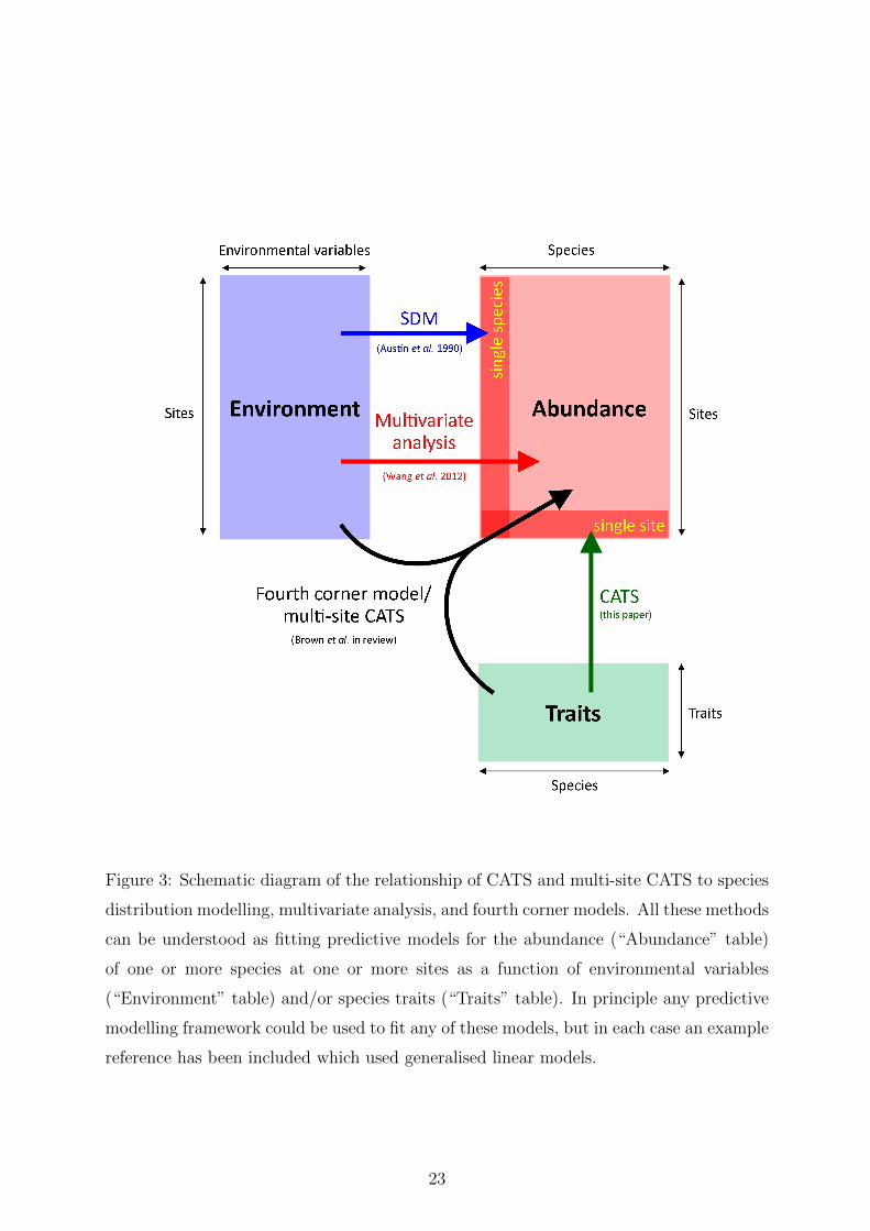
Figure 3: Schematic diagram of the relationship of CATS and multi-site CATS to species

distribution modelling, multivariate analysis, and fourth corner models. All these methods

can be understood as fitting predictive models for the abundance (“Abundance” table)

of one or more species at one or more sites as a function of environmental variables

(“Environment” table) and/or species traits (“Traits” table). In principle any predictive

modelling framework could be used to fit any of these models, but in each case an example

reference has been included which used generalised linear models.

23