CARTOGRAPHIC VISUALIZATION OF …ourspace.uregina.ca/bitstream/handle/10294/3630/Krahnen_Anne... ·...

CARTOGRAPHIC VISUALIZATION OF SASKATCHEWAN’S

POPULATION USING DASYMETRIC MAPPING

A Thesis

Submitted to the Faculty of Graduate Studies and Research

In Partial Fulfillment of the Requirements

For the Degree of

Master of Science

in

Geography

University of Regina

By

Anne Krahnen

Regina, Saskatchewan

July 2012

Copyright 2012: Anne Krahnen

UNIVERSITY OF REGINA

FACULTY OF GRADUATE STUDIES AND RESEARCH

SUPERVISORY AND EXAMINING COMMITTEE

Anne Krahnen, candidate for the degree of Master of Science in Geography, has presented a thesis titled, Cartographic Visualization of Saskatchewan's Population Using Dasymetric Mapping, in an oral examination held on May 23, 2012. The following committee members have found the thesis acceptable in form and content, and that the candidate demonstrated satisfactory knowledge of the subject material. External Examiner: Dr. Roger Wheate, University of Northern British Columbia

Co-Supervisor: Dr. Julia Siemer, Department of Geography

Co-Supervisor: Dr. Randy Widdis, Department of Geography

Committee Member: Dr. Joseph Piwowar, Department of Geography

Committee Member: Dr. Kyle Hodder, Department of Geography

Chair of Defense: Dr. Laurie Sykes-Tottenham, Department of Psychology *Not present at defense

Abstract ii

Abstract

Maps of population density are commonly displayed using the choropleth method.

Although choropleth maps are popular in mapping population density, strictly speaking,

they are often incorrect due to non-conforming boundaries of populated places and

administrative areas. This thesis looks at the dasymetric concept as an alternative to the

choropleth map and investigates how it can be applied to display Saskatchewan’s

population. Using ancillary data, the dasymetric method can redistribute statistical

population data exclusively to areas identified as populated.

As a basis for the research, 12 existing dasymetric methods were reviewed and

evaluated for their applicability to Saskatchewan. Based on this evaluation, three methods

(Binary Method, Intelligent Dasymetric Method and the Chinese Population Distribution

Model) were selected and applied to a test area (Saskatchewan’s Census Division 6). It

was assumed that the test area’s geographical attributes were representative for the

province. The ancillary dataset used for the dasymetric mapping was chosen based on the

results of regression analysis. Different file formats (raster and vector) were considered

when producing the dasymetric maps. It was observed that, due to the regular sizes of

raster cells, dasymetric maps using raster data are generally more accurate than

dasymetric maps using vector data. In the mapping process, 88 dasymetric maps were

produced for the test area. All maps were evaluated subjectively (visually), as well as

quantitatively by calculating the variations from population densities of Dissemination

Blocks (the most accurate population data available for this project) using the Mean

Abstract iii

Absolute Error. In both analyses, the binary method using raster data was determined to

be the method producing the most accurate maps for the test area.

Based on the results, three dasymetric maps were produced for the Province of

Saskatchewan. The binary method using raster data was applied at three different

resolutions (250m, 1,125m and 2,500 m). The resulting maps were therefore optimized

for three different scales (1:5,000; 1:2,250,000 and 1:5,000,000).

Keywords: Cartography; GIS; Population Maps; Dasymetric Concept; Binary Method;

Intelligent Dasymetric Method; Chinese Population Distribution Model;

Mean Absolute Error; Saskatchewan

Acknowledgements iv

Acknowledgements

It is a pleasure to thank those who made this thesis possible:

I want to thank Dr. Julia Siemer for the outstanding support and supervision during

the creation of this thesis. Thanks to her invaluable assistance, I was able to both, focus

on this project and enjoy doing the research. Dr. Siemer’s guidance helped me to make

the right decisions and leading to the successful completion of the project. Her help will

be appreciated forever.

I also want to express my gratitude to Dr. Joseph M. Piwowar for his help in

providing workspaces and software for this project. Dr. Piwowar was also very helpful in

many valuable technical discussions, which is greatly appreciated.

Special thanks to Spatial and Numeric Data Services of the Dr. John Archer

Library. Marilyn Andrews and Raye Quickfall spent countless hours in helping me to

research and access data for this project.

My thanks also goes to the Faculty of Graduate Studies and Research, particularly

for the financial support provided, which allowed me to present the results of the thesis at

the 2011 NACIS Annual Meeting in Madison, Wisconsin.

Post Defense Acknowledgements v

Post Defense Acknowledgements

I would like to thank my thesis committee for their great advice and constructive

comments:

I want to express my deep appreciation to my external examiner Dr Roger Wheate

from the University of Northern British Columbia. Thank you for your interest in my

thesis topic and for all the contributions to the discussion. I very much appreciate that you

traveled all across Canada to attend my defense.

I also thank the committee members Dr. Randy Widdis and Dr. Kyle Hodder, as

well as the chair of my defense Dr. Laurie Sykes-Tottenham for your time and valuable

ideas.

Dedication vi

Dedication

For my family and for Nima: thank you very much for supporting me throughout

the entirety of this thesis:

For my parents, who encouraged and supported me throughout my entire life; you

are my inspiration and you helped me to be the person I am today. Your support enabled

me to do what I am interested in. I am deeply thankful for knowing that you are always

there for me.

For my partner Nima; for your endless patience, encouragement and love. I would

not have been able to create this thesis if it was not for you spending countless hours

discussing it with me. Thank you for your understanding support; I am ever so grateful

for being with you.

Table of Contents vii

Table of Contents

Abstract ii

Acknowledgements iv

Post Defense Acknowledgements v

Dedication vi

Table of Contents vii

List of Tables ix

List of Figures x

List of Equations xii

List of Appendices xiv

Abbreviations xv

PART A: INTRODUCTION 1

1 Research Context 2

2 Objectives and research questions 6

3 Study Area 8

4 Limitations 15

5 Organization of the thesis 16

PART B: THE DASYMETRIC CONCEPT 18

6 The Dasymetric Concept for Mapping Population 19

7 Basic Methods 27

7.1 Areal Interpolation 27

7.2 Simple Areal Weighting 27

8 Traditional Cartographic Techniques 29

8.1 Binary Method 29

8.2 Three-Class Method and Limiting Variable Method 30

8.3 Image Texture Method 33

Table of Contents viii

9 Statistical Techniques 34

9.1 Modifying Areal Weighting 34

9.2 Expectation Maximization (EM) Algorithm 36

9.3 Inverse Distance Weighting (IDW) 36

9.4 Street-Weighting Method 37

9.5 Chinese Population Distribution Model (CPDM) 38

9.6 Cadastral-based Expert Dasymetric System (CEDS) 41

9.7 Intelligent Dasymetric Mapping (IDM) 43

PART C: APPLICATION 45

10 Methods 46

11 Data 50

11.1 Statistical data and administrative areas 50

11.2 Ancillary Data 53

12 Regression Analysis 56

13 Binary Method 59

14 Intelligent Dasymetric Mapping 62

15 Chinese Population Distribution Model 63

PART D: ANALYSIS 71

16 Results 72

17 Evaluation 88

17.1 Visual Evaluation 88

17.2 Statistical Evaluation 92

18 Dasymetric map for Saskatchewan 99

19 Conclusions 103

20 Future Research 105

21 Appendix 107

22 References 119

22.1 Literature 119

22.2 Map data sources 123

List of Tables ix

List of Tables

Table 3.1: Characteristics of the test area, Saskatchewan's Census Division

No. 6 (Statistics Canada, 2007 a) 12

Table 6.1: An overview of dasymetric mapping techniques 25

Table 10.1: Categorization of dasymetric methods 47

Table 11.1: Statistics Canada's definitions for the administrative areas used

(Statistics Canada, 2010) 51

Table 12.1: OLS model for GeoBase LandCover ca. 2000 58

Table 15.1: Classification of land cover classes for CPDM 66

Table 15.2: Results of the univariate regression analysis with habitable land

cover classes and rural population 67

Table 16.1: Results of the application of the dasymetric methods to the test area 72

Table 17.1: Visual Evaluation of dasymetric maps created for the test area 91

Table 17.2: Numeric evaluation of dasymetric maps created with CSD and

LandCover ca. 2000 data 95

List of Figures x

List of Figures

Figure 1.1: Comparison between dasymetric method (left) and choropleth

method (right) (Mennis, 2009, p. 740) (original in colour) 5

Figure 2.1: Population Density of Saskatchewan's Dissemination Blocks in

Northern Saskatchewan, Regina and Saskatoon (original in colour) 7

Figure 3.1: Populated places in Saskatchewan (original in colour) 11

Figure 3.2: Population Density of the Dissemination Blocks within the Test Area -

Saskatchewan's CD6 13

Figure 3.3: Test Area: Census Division No. 6 within Saskatchewan (original in

colour) 14

Figure 5.1: Organization of the thesis 16

Figure 6.1: Population density map of Ireland produced in 1837 by Henry

Drury Harness (Robinson, 1955). 20

Figure 6.2: The dasymetric concept for population distribution modeling

(modified after Langford, 2003, p. 143) 22

Figure 8.1: Concept of the Binary Method 30

Figure 8.2: Concept of the Three-Class Method 31

Figure 8.3: Concept of the Limiting Variable Method 32

Figure 11.1: Standard Census and Geographic Units 2006 (Statistics Canada,

2007 c) 51

Figure 13.1: Binary Method with vector data 60

Figure 13.2: Binary Method with raster data 61

Figure 15.1: Cell-based encoding method of percentage breakdown (CPDM) 65

Figure 15.2: Calculation of the distance of each urban cell to the centre of its

urban area (CPDM) 69

Figure 16.1: Dasymetric map created with the Binary Method (raster),

LandCover ca. 2000, and CCS (original in colour) 73


LandCover ca. 2000, and CSD (original in colour) 74


LandCover ca. 2000, and DA (original in colour) 75

List of Figures xi

Figure 16.4: Dasymetric map created with the Binary Method (vector),

LandCover ca. 2000, and CSD (original in colour) 76

Figure 16.5: Dasymetric map created with the Binary Method (raster), Buildings

and Structure Theme from CanVec (NRCan), and CSD (original in

colour) 77

Figure 16.6: Dasymetric map created with the Binary Method (raster), Land

Cover 2005 (North American Environmental Atlas), and CSD

(original in colour) 78

Figure 16.7: Dasymetric map created with the Binary Method (raster), Street

Network Density (CanVec), and CSD (original in colour) 79

Figure 16.8: Dasymetric map created with the IDM (Centroid Method; Sample

Size 5), LandCover ca. 2000, and CSD (original in colour) 80


Sizes 20), LandCover ca. 2000, and CSD (original in colour) 81


Sizes 30, 40, 50, 75), LandCover ca. 2000, and CSD (original in

colour) 82

Figure 16.11: Dasymetric map created with the IDM (Containment Method;

Sample Sizes 5, 20, 30, 40, 50, 75), LandCover ca. 2000, and CSD

(original in colour) 83

Figure 16.12: Dasymetric map created with the IDM (Percent Coverage Method

70%: Sample Size 5, LandCover ca. 2000, and CSD (original in

colour) 84


80%: Sample Size 5, LandCover ca. 2000, and CSD (original in

colour) 85


(90%, 100%: Sample Size 5) and (70%, 80%, 90%, 100%, Sample

Sizes: 20, 30, 40, 50, 75), LandCover ca. 2000, and CSD (original

in colour) 86

Figure 16.15: Dasymetric map created with the CPDM, LandCover ca. 2000, and

CSD (original in colour) 87

Figure 18.1: Comparison of details of dasymetric maps (created with the binary

method and various resolutions) and the corresponding choropleth

maps (original in colour) 102

List of Equations xii

List of Equations

Equation 7.1: Simple Areal Weighting (Langford, 2006) 28

Equation 8.1: Binary Dasymetric Method (Langford, 2006) 29

Equation 8.2: Three-Class Method (Langford, 2006) 31

Equation 9.1: Population densities for land cover classes of administrative area

(Modifying Areal Weighting Method) (Bielecka, 2005) 34

Equation 9.2: Difference indicator for the region (Modifying Areal

Weighting Method) (Bielecka, 2005) 35

Equation 9.3: Correlation between the known and estimated population

densities, as well as the area of a land use class and the total area

of an administrative area (Modifying Areal Weighting Method)

(Bielecka, 2005) 35

Equation 9.4: Population density after the Modifying Areal Weighting Method:

new weighting coefficient (Bielecka, 2005) 35

Equation 9.5: Inverse-distance weighting (Slocum et al., 2009) 37

Equation 9.6: Street weighting method (Reibel & Bufalino, 2005) 38

Equation 9.7: Chinese Population Distribution Model (CPDM) (Tian et al.,

2005) 39

Equation 9.8: Regression model to calculate rural population (CPDM) (Tian et

al., 2005) 39

Equation 9.9: Order of rural probability coefficients (CPDM) (Tian et al.,

2005) 40

Equation 9.10: Rural population probability coefficient for CPDM (Tian et al.,

2005) 40

Equation 9.11: Urban population probability coefficient for CPDM (Tian et al.,

2005) 41

Equation 9.12: Dasymetrically derived population of a cadastre (CEDS)

(Maantay et al., 2007) 42

Equation 9.13: Difference of estimated and true population of smaller

administrative units (CEDS) (Maantay et al., 2007) 42

Equation 9.14: Redistribution of data for Intelligent Dasymetric Mapping

(IDM) (Mennis & Hultgren, 2006) 43

List of Equations xiii

Equation 9.15: Calculation of population density of ancillary classes for IDM

(Mennis & Hultgren, 2006) 44

Equation 15.1: Rural probability coefficient (CPDM) 67

Equation 15.2: Urban probability coefficient (CPDM) 68

Equation 15.3: CPDM for urban areas 70

Equation 15.4: CPDM for rural areas 70

Equation 15.5: Calculation of population density of CPDM 70

Equation 17.1: Difference in population density between DB and dasymetric

areas 93

List of Appendices xiv

List of Appendices

I. LIST OF POTENTIAL ANCILLARY DATA 107

II. OLS RESULTS 110

OLS model for LandCover 2005 of the North American Environmental

Atlas 110

OLS model for the Buildings and Structure Theme of CanVec by NRCan 111

III. NUMERIC RESULTS 112

Numeric Evaluation of dasymetric maps created with the binary method and

vector data 112

Numeric Evaluation of dasymetric maps created with the binary method and

raster data 112

Numeric Evaluation of dasymetric maps created with the IDM, the Centroid

Method and LandCover ca. 2000 data 113

Numeric Evaluation of dasymetric maps created with the IDM, the

Containment Method and LandCover ca. 2000 data 114

Numeric Evaluation of dasymetric maps created with the IDM, the Percent

Coverage Method and LandCover ca. 2000 data 114

Numeric Evaluation of dasymetric map created with the CPDM, Census

Subdivisions and LandCover ca. 2000 data 116

IV. ARCGIS 10.X TOOLS 117

List of ArcGIS 10 tools used to create the dasymetric maps 117

V. DASYMETRIC MAPS OF SASKATCHEWAN 118

Abbreviations xv

Abbreviations

ANOVA Analysis of Variance

CCS Census Consolidated Subdivision

CD Census Division

CEC Commission for Environmental Cooperation

CEDS Cadastral-based Expert Dasymetric System

CMA Census Metropolitan Area

CORINE Coordination of information on the environment

CPDM Chinese Population Distribution Model

CSD Census Subdivision

DA Dissemination Area

DB Dissemination Block

DEM Digital Elevation Model

DLI Data Liberation Initiative

EM Expectation-Maximization

ESRI Environmental Systems Research Institute

GIS Geographic Information System

GRASS Geographic Resources Analysis Support System

IDM Intelligent Dasymetric Mapping

IDW Inverse Distance Weighting

MAE Mean Average Error

MAUP Modifiable Areal Unit Problem

OLS Ordinary Least Squares

Q-GIS Quantum Geographic Information System

RMS Root Mean Square

VBA Visual Basic for Application

PART A:

INTRODUCTION

About the research and about Saskatchewan as the study area


1 Research Context

Not only is it easy to lie with maps, it’s essential. [...] There’s no

escape from the cartographic paradox: to present a useful and

truthful picture, an accurate map must tell white lies.

(Monmonier, 1996, p. 1)

Society employs maps as common and effective visual modes of communication.

During the mapping process, cartographers try to accomplish what seems to be

impossible: to present meaningful relationships of phenomena occurring in our three-

dimensional complex world in a two-dimensional format (i.e. paper or screen). Thus

maps are only able to show a generalized picture of our world: relevant objects are

selected, less important objects are omitted; objects of same groups are merged; some

objects are emphasized while others are not. There are established rules for these

generalizations and selections but while some of them are intentionally misleading, others

are simply unavoidable and necessary due to the method applied, the mapping scale, or

the complexity of the map.

In this context, a discussion amongst cartographers about the correct representation

of population using maps arose in the 1980s. In contemporary thematic cartography,

population density is most often displayed using the choropleth method, one of the most

common cartographic methods in the field of thematic mapping (Slocum et al., 2009).

The International Cartographic Association has defined the choropleth method as “a

method of cartographic representation which employs distinctive colour or shading

applied to areas other than those bounded by isolines. These are usually statistical or

administrative areas” (Dent, 1999, p. 139). Typically, the choropleth method is used to


display statistical data for enumeration units. These units are commonly determined by

official censuses or statistical agencies. The choropleth method is typically applied in

population mapping by classifying ratio data, such as population density.

A characteristic of choropleth maps is the abrupt change of values at the

enumeration unit boundaries (Slocum et al., 2009). Thus, the application of the

choropleth method is only truly appropriate for phenomena, whose values change at these

boundaries (e.g., tax rates). Consequently, in theory the choropleth method is not suitable

for phenomena whose real distribution is not reflected by the boundaries of

administrative areas (e.g., population). Langford and Unwin (1994) identified and

described three of the major problems of the choropleth method: first, there is a trend to

use larger areal units for data collection. This results in a simplification where both,

unpopulated and populated areas are frequently combined in a single areal unit,

producing underestimates of population density values. This leads to the second issue

defined as generalization. When large enumeration areas are used, variations occurring

within the choropleth boundaries cannot be shown and the true distribution of data is lost.

The third problem is known as the Modifiable Areal Unit Problem (MAUP). This was

first described by Openshaw in 1984 and refers to different results when one topic is

mapped using different areal units (Langford & Unwin, 1994). To solve some of these

problems, the use of smaller administrative areas is recommended (Raisz, 1962).

Research in the field of thematic cartography is not unfamiliar with the discussion

of the limitation and problems associated with the choropleth method. The choropleth

concept was first applied in 1826 and quickly became one of the most popular


cartographic methods (Crampton, 2004). Due to the limitations of the choropleth method

to political boundaries, its application was limited in 1938 by cartographers such as Raisz

and Wright (Crampton, 2004). Subsequently, the concept of the dasymetric method was

re-introduced and for a short time it became widespread and well known amongst

cartographers (Crampton, 2004). The dasymetric method tries to display a more true

distribution than the choropleth method (figure 1.1). This is accomplished by using

additional, so-called ancillary data, such as land-cover or slope data. Although the

concept is clear and simple, the realization and implementation of the method is

complicated. This complexity leads to unanswered questions (about e.g. ancillary data,

data formats, or redistribution techniques), which are responsible for a lack of a

standardized dasymetric method today. Since the late 1980s, progress in two geo-spatial

technologies, geographic information systems (GIS) and remote sensing, has helped to

move this neglected technique back in the centre of cartographic research. Cartographers

have now developed several dasymetric methods to display population density and

distribution to help understand underlying patterns.


Figure 1.1: Comparison between dasymetric method (left) and choropleth method (right) (Mennis, 2009,

p. 740) (original in colour)

Even though the dasymetric concept is applicable to different phenomena, research

in dasymetric mapping tends to focus on improving population maps. Population maps

are important since they are not only used for monitoring local and global population, but

are also used in fields such as health studies and environmental justice, crime statistics,

research on different social and racial groups, emergency planning and management, and

accessibility to social services (Mennis, 2009). Population distribution refers to the

arrangement of people living in a certain region, while population density is the ratio of a

population to a predefined area (Mayhew, 2004).


2 Objectives and research questions

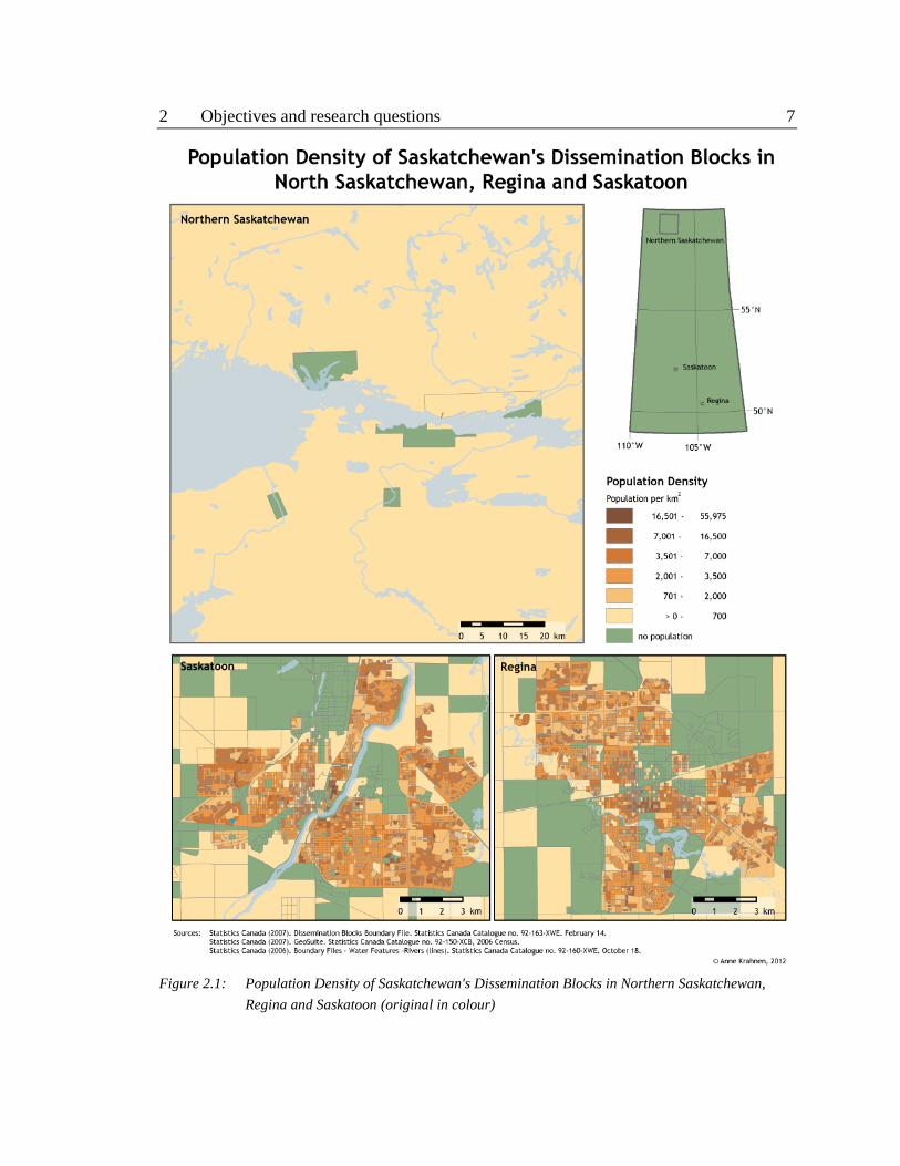
In Saskatchewan, population maps are commonly created with the choropleth

method. Even when these maps use the smallest administrative areas of the 2006

Statistics Canada census, the Dissemination Blocks (DB), they only deliver an acceptable

visual representation of population distribution and population density for urban areas

such as Regina or Saskatoon (figure 2.1). In the rural areas of the province, the largest of

these administrative areas has a size of more than 48,000 km2 while its population was 84

people in the census of 2006. Using the choropleth method, this area would be mapped

with a population density of zero, ignoring the fact that there are people living there. For

cartographic purposes, this requires some enhancement (figure 2.1). The dasymetric

method has the ability to show a more realistic map of the distribution and density of

population density by excluding the uninhabited areas. Most dasymetric methods have

been applied to densely settled areas or big cities, while few have been applied to large

sparsely inhabited areas (cf. chapter 6). The goal of this thesis project is to apply the

dasymetric concept to Saskatchewan and to evaluate the map’s ability to show the

province’s population distribution and population density.

The research of this thesis project addresses the following questions: can the

dasymetric concept be applied to cartographically represent the population of

Saskatchewan more effectively than choropleth mapping? Which of the existing methods

provides the best results? Does the dasymetric method improve the visual representation

of Saskatchewan’s population? What are the problems when the dasymetric method is

applied to Saskatchewan? Which ancillary data deliver the most accurate results?


Figure 2.1: Population Density of Saskatchewan's Dissemination Blocks in Northern Saskatchewan,

Regina and Saskatoon (original in colour)

3 Study Area 8

3 Study Area

Saskatchewan’s population is distributed very unevenly throughout the province. In

the Census of 2006, Saskatchewan had a total population of 968,157 inhabitants and an

overall population density of 1.6 persons per km2 (Statistics Canada, 2007 c). Since 2006,

the population has increased and provincial estimates calculated a population of

1,053,960 inhabitants for April 1st, 2011 (Government of Saskatchewan, 2011). In the

census of 2006, 65 percent of Saskatchewan’s population lived in urban places1

(Government of Saskatchewan, 2010) and 40 percent lived in the metropolitan areas of

Regina and Saskatoon (Thraves, 2007). The remaining 35 percent (339,244 people) of the

total population was identified as rural, living in isolated farmsteads, villages, group

settlements, as well as First Nations and Métis settlements. Based on the definition

provided by Statistics Canada, Saskatchewan had 15 cities, 145 towns, 306 villages and

296 rural municipalities as of July 2010 (Government of Saskatchewan, 2011).

A large part of Saskatchewan’s population (98.7 percent) is located south of the

54th

latitude (figure 3.1). During the time of the province’s early settlement, most urban

settlements were built along railway lines and this structure is still observable. Regina

(179,246 inhabitants in 2006) and Saskatoon (202,340 inhabitants in 2006) are

Saskatchewan’s largest cities (Government of Saskatchewan, 2007). Together they

1 According to Statistics Canada (2010), a settlement reaches the urban status when its population counts

more than 1,000 people and its population density is higher than 400 people per km2. Cities are defined as

urban places having a population of at least 5,000 people. In contrast, rural population is defined as the

regions lying outside of urban areas.

3 Study Area 9

embrace 39.4 percent of Saskatchewan’s total population and 60.7 percent of

Saskatchewan’s urban population. Furthermore, the Census Metropolitan Areas (CMA)

of these two cities hold 44.3 percent of Saskatchewan’s population. In Saskatchewan, no

cities of intermediate size (50,000 to 150,000 inhabitants) exist. Prince Albert (34,138)

and Moose Jaw (32,132) are the next largest cities and have significantly fewer

inhabitants (Government of Saskatchewan, 2007).

Although Regina and Saskatoon account for most of Saskatchewan’s urban

population, their share of Saskatchewan’s urban area is at 29.6 percent comparatively

small. This ratio of high population to small area produces relatively high population

densities of 1,184.4 people per km2 in Saskatoon and 1,507.9 people per km

2 in Regina

(Thraves, 2007). In comparison, the population densities of the smaller urban areas are

lower. The city of Prince Albert has the lowest population density with 519.7 persons per

km2. Towns with less than 5,000 inhabitants embrace 37.1 percent of Saskatchewan’s

urbanized area but only account for 16.4 percent of the urban population (Thraves, 2007).

There are different kinds of rural settlements in Saskatchewan; most of them are

agricultural. The dominant type is the isolated farmstead, but there are also farm villages,

as well as group farmsteads; most Aboriginal settlements are also considered rural.

Farming is predominantly restricted to the lands south of the parkland belt or boreal

forest fringe (treed and forested classes in figure 3.2). The density and distribution of

rural settlements, especially isolated farmsteads, depend on farm sizes. In the southwest

and northwest, the density is very low due to larger farms, while the farms in the

3 Study Area 10

northeast of the province and close to the cities of Regina and Saskatoon are smaller and

the density higher (Schlichtmann, 2007).

3 Study Area 11

Figure 3.1: Populated places in Saskatchewan (original in colour)

3 Study Area 12

Due to the complexity of the dasymetric mapping process, the methods selected for

this research were tested by first applying them to a portion of the province.

Saskatchewan’s Census Division (CD) No. 6 (figure 3.3) was chosen as the test area

because it has characteristics that can challenge the dasymetric method (e.g. the abrupt

changes between densely settled areas and unsettled regions), at the same time as being

generally representative of the variations of different settlements and structures that are

observable characteristics throughout the province (table 3.1 and figure 3.1). The

variation of population densities of the Dissemination Blocks (DB) within the Census

Division (zero persons per km2 in rural areas and 20,058 persons per km

2 in Regina) is

also representative of the province’s uneven population distribution (figure 3.2). Its close

proximity to the University of Regina facilitated a familiarity with this region that was

useful in the interpretation of the results.

Table 3.1: Characteristics of the test area, Saskatchewan's Census Division No. 6 (Statistics Canada,

2007 a)

Size 17,548 km2

Total population 220,688

Settlement structure 1 city

15 towns

30 villages

14 resort villages

20 rural municipalities

12 First Nations reserves

3,500 farms

Administrative areas 21 Census Consolidated Subdivisions

92 Census Subdivisions

435 Dissemination Areas

5,707 Dissemination Blocks

3 Study Area 13

Figure 3.2: Population Density of the Dissemination Blocks within the Test Area - Saskatchewan's CD6

3 Study Area 14

Figure 3.3: Test Area: Census Division No. 6 within Saskatchewan (original in colour)

4 Limitations 15

4 Limitations

The purpose of this thesis is to examine how existing dasymetric techniques can be

applied to mapping the population density of Saskatchewan. The test area was chosen to

minimize errors occurring due to calculations with large data, as well as limitations in

computing resources. Regional models, that generate dasymetric models using different

parameters for different regions, were not considered. Dasymetric methods were applied

without any modification from their originally published descriptions. This means that

there is no new dasymetric mapping approach introduced in this thesis.

This thesis does not apply all dasymetric methods and not all available ancillary

data were tested and used. The dasymetric methods were selected systematically using

predetermined criteria (cf. chapter 10), while regression analysis was used to chose the

ancillary data that correlate best to population density (cf. chapter 11.2).

The dasymetric maps created in this thesis were evaluated using the Mean Absolute

Error (MAE) (cf. chapter 17.2). For the MAE, the dasymetric maps were compared to the

choropleth maps of the smallest areal unit available to the research, Dissemination Blocks

(DB). Although not ideal, this is the standard approach as population data of better

precision are generally not available.


5 Organization of the thesis

Figure 5.1: Organization of the thesis


This thesis is organized in 4 Parts (figure 5.1):

The first five chapters (Part A) introduce the topic.

Part B describes the dasymetric concept and extends from chapter 6 through 9.

Chapter 6 introduces the concepts of dasymetric mapping. In addition to the historical

background of dasymetric mapping, different mapping techniques are reviewed and

presented. A system to categorize dasymetric methods is introduced and applied in

chapters 7 through 9.

Part B is the foundation for the further research conducted in Part C. Chapter 10

describes how the dasymetric methods are chosen for the research, while chapter 11

discusses the ancillary and statistical data that are considered. The regression analysis in

chapter 12 is used to determine which of the data chosen in chapter 11 are most suitable

for dasymetric mapping. Chapters 13 through 15 provide a description of how the binary

method, the IDM and the CPDM are applied to the test area.

In part D, the results of the research are presented. The results are evaluated

visually and statistically in chapter 17. Based on this evaluation, final maps are presented

in chapter 18 and the thesis’ conclusions are presented in chapter 19. Ideas for future

research based on the results of this thesis are introduced in chapter 20.

Map generation was done using ArcGIS 10. For a comprehensive list of tools used,

see appendix IV.

PART B:

THE DASYMETRIC

CONCEPT

A literature review

6 The Dasymetric Concept for Mapping Population 19

6 The Dasymetric Concept for Mapping Population

The dasymetric concept is part of the cartographic methods for displaying statistical

surfaces. Phenomena and variables that vary continuously over space are usually

displayed using this concept. The distribution of these phenomena is mostly independent

from political or administrative boundaries. Typically, the dasymetric concept is applied

to population. The dasymetric concept suggests that the distribution and density of

population can be explained logically using so-called ancillary data. By analyzing the

relationship between ancillary data and population, dasymetric maps are able to show

distinct distributions, as well as peak values and local variations (Mennis, 2009).

Although there are numerous dasymetric mapping approaches, there is no standardized

dasymetric method. Hence, a generally accepted valid relationship between ancillary data

and statistical surfaces remains to be defined. The challenge therefore is how to use

statistical data (e.g., census data), redistribute them to populated areas, and determine the

population density.

There are different theories about the historical roots of the dasymetric concept and

assumptions are made that it has been reinvented more than once (Mennis, 2009). It is

believed that the 1833 world map by Julius Poulette Scrope and the population density

map of Ireland produced in 1837 by Henry Drury Harness (figure 6.1), are the earliest

examples of maps showing approaches of the dasymetric concept (Petrov, 2008).

However, in 1833 and 1837, the dasymetric concept had not yet been described or

named. Poulette Scrope’s and Drury Harness’s works are acknowledged for recognizing

the problems associated with the choropleth method (Mennis, 2009).

6 The Dasymetric Concept for Mapping 20

Figure 6.1: Population density map of Ireland produced in 1837 by Henry Drury Harness (Robinson,

1955).

The Russian cartographer Semenov-Tian-Shanski was the first to name, publish and

talk about the concept of dasymetric mapping. According to Semenov-Tian-Shanski the

name ‘dasymetric’ is a Russian translation and modification of the Greek term for

‘density measurement’ and was introduced in Semenov-Tian-Shanski’s report to the

Russian Geographic Society in 1911 (Petrov, 2008). In this article, he also provided a


first definition describing “dasymetric maps as those on which population density,

irrespective of any administrative boundaries, is shown as it is distributed in reality, that

is, by natural spots of concentration rarefaction” (Benjamin Semenov-Tian-Shanski as

quoted in and translated by Petrov, 2008, p. 134). After Semenov-Tian-Shansky’s

publication ‘Dasymetric Map of European Russia’ in 1923, the dasymetric mapping

technique became extremely popular throughout the former Soviet Union. For reasons,

which are unknown today, the concept nevertheless disappeared as fast as it appeared

from the vocabulary of cartographers (Petrov, 2008). De Geer, who reviewed Semenov-

Tian Shansky’s work, first introduced the dasymetric concept to Anglophone

cartographers (de Geer, 1926). In 1928, Semenov-Tian-Shansky himself published an

article in the same journal, also introducing the concept and its benefits (Semenov-Tian-

Shansky, 1928). Mistakenly, current research gives credit to J.K. Wright for inventing

and introducing the dasymetric concept to Anglophone cartographers. In 1936, Wright

published an article discussing population mapping, the advantages and disadvantages of

several methods, and their application to Cape Cod, a region in Eastern Massachusetts.

While he acknowledged and referred to the Russian roots of the method, he did not

mention Semenov-Tian-Shansky’s work (Wright, 1936).

In 1969, McCleary provided a definition for dasymetric mapping. This definition is

generally accepted and currently used: “Simply defined, the dasymetric method portrays

a statistical surface as a series of zones of uniform statistical value separated by

escarpments of rapid change in values (i.e., zones or high gradient)” (McCleary, 1969 as

quoted in Dent, 1999).


Recent research on dasymetric mapping links this cartographic concept to areal

interpolation techniques. Areal interpolation is defined as “the transfer of data from one

set (source units) to a second set (target units) of non-hierarchical, areal units” (Gregory,

2002, p. 295). Based on this definition, dasymetric mapping is an areal interpolation

technique.

Generally, current research on the dasymetric concept seeks to define a universally

valid correlation of statistical surface and ancillary data (figure 6.2). Besides the

methodology of how to determine the functional relationship between those datasets, the

application and results of using different ancillary data is examined: While land use or

land cover data are used traditionally, the integration of light-emission data (Briggs et al.,

2007), pixel maps (Langford, 2007), postal codes (Langford et al., 2008), street networks

(Reibel & Bufalino, 2005), or elevation (Liao et al., 2008) are also examined.

Figure 6.2: The dasymetric concept for population distribution modeling (modified after Langford, 2003,

p. 143)


Ever since the dasymetric concept was invented, cartographers believe that the

application of this method can solve problems that occur when irregularly distributed

phenomena (e.g., population) are mapped with the choropleth method. All methods

applied to display population distribution and density are supposed to preserve the so-

called pycnophylactic property (Tobler, 1979). According to the pycnophylactic property,

the total population of a region has to remain the same when population is redistributed to

dasymetric areas (Reibel & Bufalino, 2005).

In spite of the potential of the dasymetric concept, it has never achieved a high

popularity. For a long time, awareness of the dasymetric concept amongst cartographers

was very low. Complexity, technical difficulty, lack of standardization, and unavailability

of data are a few reasons for this. With the development and advanced abilities of GIS

and remote sensing beginning in the 1980s, cartographers and scholars are gradually

becoming more aware of the dasymetric concept and its advantages over other

cartographic techniques. Since then, many papers and articles have been published

discussing dasymetric mapping and much effort has been made towards the development

of a standardized technique (Eicher & Brewer, 2001).

Due to different spatial patterns of population distribution and population density, a

variety of dasymetric methods have been developed. Most of them are appropriate for the

application to areas with certain characteristics (e.g., size, population density, population

distribution, spatial pattern, etc.). The methods also use different ancillary data for

dasymetric mapping. In 2009, Mennis classified dasymetric methods in traditional

cartographic techniques and statistical techniques (table 6.1). Amongst others, the


traditional cartographic techniques embrace the binary method, three-class method, and

the limiting variable method. All these methods have in common that their principles are

rooted in the basic concepts of cartography. The author of the map ideally considers

previous knowledge of the area and determines the functional relationship between

statistical surface and ancillary data subjectively. Statistical techniques in contrast relate

to areal interpolation techniques, establishing the relationship between ancillary data and

statistical surface based on existing data and their internal patterns. These techniques do

not require subjective decisions or previous knowledge of the area. Mennis (2009)

therefore claims that they work “in a more sophisticated manner than the traditional

cartographic approaches” (Mennis, 2009, p. 733).

A variety of dasymetric mapping methods exist. Table 6.1 gives a brief overview of

techniques discussed most commonly in recent literature. The classification by Mennis

(2009) is therefore modified. A third group of methods, the Basic methods are

introduced. Strictly speaking, Basic methods are not dasymetric as they do not require the

use of ancillary data. Nevertheless, they are included since they provide the basic

concepts for most of the other dasymetric mapping methods:


Table 6.1: An overview of dasymetric mapping techniques

Method Principles Discussed and applied by:

Bas

ic M

eth

od

s

Simple Areal

Weighting

Population is redistributed based

on the proportion of the source

zone, which belongs to the target

zone. Ancillary data are not

needed.

Briggs, Gulliver, Fecht & Vinneau, 2007

Gregory, 2002

Eicher & Brewer, 2001

Fisher & Langford, 1996

Areal

Interpolation

Control zones are used to

transform data from choropleth

zones to target zones. The

dasymetric zones do not

necessarily match with

choropleth zones or ancillary

data.

Liao, Wang, Meng & Li, 2008

Maantay, Maroko & Hermann, 2007

Reibel & Bufalino, 2005

Fisher & Langford, 1996

Tra

dit

ion

al C

arto

gra

ph

ic T

echn

iqu

es

Binary

Method

Population is exclusively

reassigned to areas identified

populated. An equal population

distribution within dasymetric

areas is assumed.

Mennis, 2009

Bielecka, 2005


de Geer, 1926

Three-Class

Method

Based on the characteristics of

the dasymetric zones, a

percentage of the population is

assigned to them.

Mennis, 2009



Limiting

Variable

Method

A maximum population density

is determined for each

dasymetric zone. Based on these

limits population is redistributed,

from rural to urban areas.


Gregory, 2002


McCleary, 1969

Image

Texture

Method

Identification of populated and

unpopulated areas based on

scanned reference maps.

Langford, Higgs, Radcliffe & White, 2008

Langford, 2007



Method Principles Discussed and applied by: S

tati

stic

al T

ech

niq

ues

Modifying

Areal

Weighting

Regression models are used to

find the relationship between

land-cover classes and

population density.

Briggs, Gulliver, Fecht & Vinneau, 2007

Langford., 2007

Bielecka, 2005

Gallego & Peedell, 2001

Expectation

Maximization

(EM)

algorithm

The algorithm uses areal

weighting techniques to

redistribute data from choropleth

zones to dasymetric zones. Using

maximum likelihood, the

population density is calculated

for each dasymetric zone.

Mennis, 2009

Langford, 2007

Mennis & Hultgren, 2006

Gregory, 2002

Inverse

distance

weighting

(IDW)

Population counts are assigned to

the centroids of the

administrative areas. Population

is assigned to areas around the

centroid assuming decreasing

density.

Liao, Wang, Meng & Li, 2008

Mennis, 2003

Street

weighted

method

Street networks are used to

gather weights for the

interpolation of population

density surfaces.



Reibel & Bufalino, 2005

Chinese

population

distribution

model

(CPDM)

Population is redistributed for

Agro-ecological zones

individually based on population

probability coefficients. The

model uses land cover data and

distinguishes between urban and

rural population.

Tian, Yue, Zhu, & Clinton, 2005

Cadastral-

based Expert

Dasymetric

System

(CEDS)

This method uses tax lot

(cadastral) data as ancillary data

to improve dasymetric mapping

in the urban environment.

Maantay & Maroko, 2009


Intelligent

Dasymetric

Method

(IDM)

Combines a variety of techniques

to determine the relationship

between ancillary data and

statistical surface

Mennis, 2009


7 Basic Methods 27

7 Basic Methods

7.1 Areal Interpolation

Areal interpolation has been defined as “the transfer of data from one set (source

units) to a second set (target units) of overlapping, non-hierarchical, areal units"

(Langford et al., 1991, p. 57). The technique was developed as a general statistical

method not focused on map production. Its original purpose is to create comparability of

dataset using different enumeration units. Areal interpolation enables the transfer of a

dataset to a common set of enumeration units (Eicher & Brewer, 2001). Based on this

definition, dasymetric mapping methods are a specification of areal interpolation

techniques.

7.2 Simple Areal Weighting

Simple areal weighting is the simplest and the most commonly applied form of

areal interpolation (Fisher & Langford, 1996). This method does not require ancillary

information and is simply based on the geometric intersection of the source and target

zones. It assumes an equal distribution of population throughout the source zone. The

amount of population assigned to the target zones is assumed proportional to the target

zone’s portion of the source zone (equation 7.1; Langford, 2006). Eicher and Brewer

(2001) suggest that simple area weighting should not be used for dasymetric mapping, as

it does not use ancillary data. The method nevertheless is used in a variety of studies but

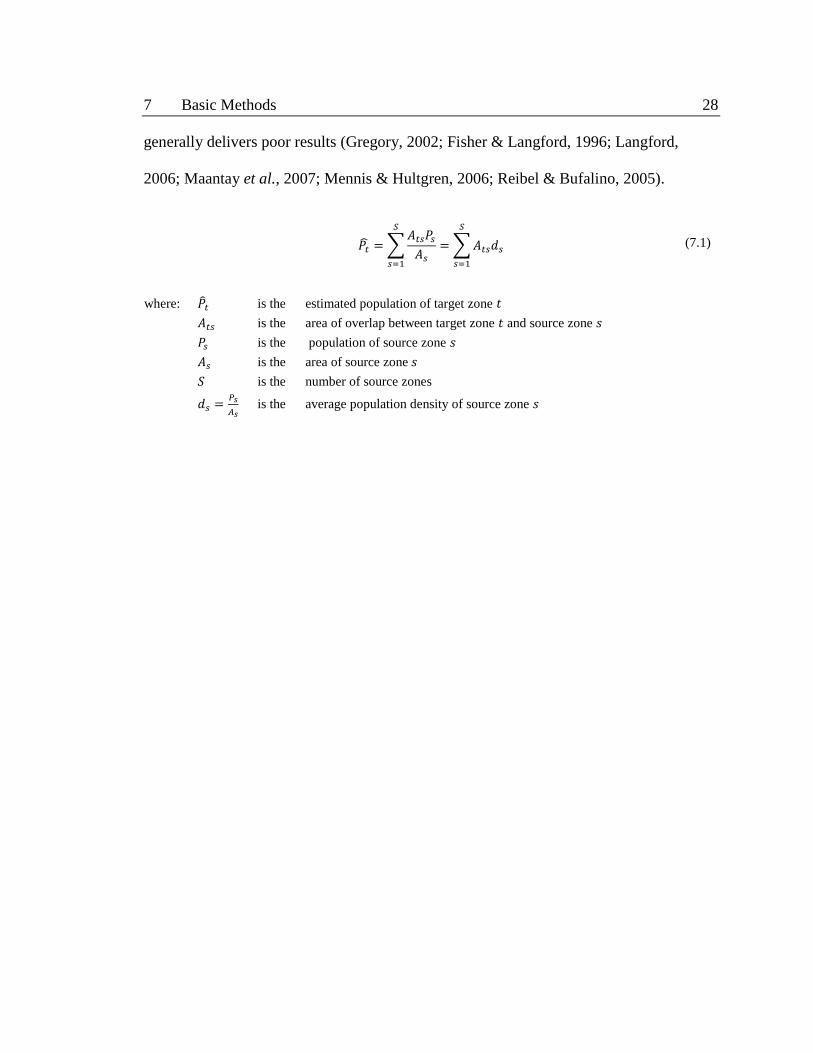
7 Basic Methods 28

generally delivers poor results (Gregory, 2002; Fisher & Langford, 1996; Langford,

2006; Maantay et al., 2007; Mennis & Hultgren, 2006; Reibel & Bufalino, 2005).

∑

∑

(7.1)

where: is the estimated population of target zone

is the area of overlap between target zone and source zone

is the population of source zone

is the area of source zone

is the number of source zones

is the average population density of source zone

8 Traditional Cartographic Techniques 29

8 Traditional Cartographic Techniques

8.1 Binary Method

The binary method is a simplistic approach of dasymetric mapping and has been

applied to combine land use/ land cover data with the statistical surface. It is expressed

with the following formula (equation 8.1):

∑

∑

(8.1)


is the area of overlap between target zone and source zone , and having land

cover identified as populated


is the area of source zone having land cover identified as populated


is the dasymetric density of the populated class in source zone

The land use/ land cover classes are determined to be either inhabitable or

uninhabitable areas. The population of the source zones is equally redistributed to the

target zones (figure 8.1) (Slocum et al., 2009). Even though the binary method is a very

basic method, it has the ability to create accurate and realistic maps in several tests and

case studies (Eicher & Brewer, 2001; Fisher & Langford, 1996).

Although the method is easy to apply, it requires subjective decisions when

inhabitable and uninhabitable areas are identified. The binary method also does not

distinguish between different population densities within populated areas and eliminates

7 Basic Methods 30

all population from areas identified as uninhabited. This does not necessarily reflect the

actual situation (Maantay et al., 2007).

Figure 8.1: Concept of the Binary Method

8.2 Three-Class Method and Limiting Variable Method

The three-class method, like the limiting variable method, is based on the concepts

of the binary method. The three-class method is a first step to considering variations in

population density (e.g., between rural and urban areas) (Langford, 2006). Applying this

method, the (three) major land-use categories containing population are identified.

Population is assigned exclusively to these areas. In a next step, the percentage of the

population living in those land-cover classes is determined (e.g., 70 percent lives in class

1, 20 percent lives in class 2, and 10 percent lives in class 3). Based on these percentages,

the population is redistributed to the dasymetric zones assuming an equal population

distribution within each zone (equation 8.2 and figure 8.2). Even though this method

takes different population densities of land-use categories into account, it still does not

consider variations within classes. This can be problematic when a high percentage of

population is assigned to very small areas (Maantay et al., 2007).

7 Basic Methods 31

∑∑

∑∑

(8.2)


is the area of overlap between target zone and source zone , and having land

cover identified as populated class


is the area of source zone having land cover identified as populated class


is the number of populated land cover classes

is the dasymetric density of the populated class in source zone

Figure 8.2: Concept of the Three-Class Method

The limiting variable technique is based on the dasymetric concept published by

Wright in 1936 and further refines the three-class method (Slocum et al., 2009). Like the

three-class method, this method also identifies the (three) major inhabited land-use

classes to which population are assigned. Unlike the three-class method, however, the

limiting variable method determines a maximum population density for the land-use

classes. Usually there is no limit to the population density of urban classes. The

redistribution process starts by assuming an equal population distribution throughout all

dasymetric zones. In a next step, the population density and threshold of the land use

7 Basic Methods 32

class with the lowest threshold are compared. If the population density exceeds the

threshold, the exceeded population is assigned to the remaining areas. This process is

repeated for every zone. At the end, the remaining population will be assigned to areas

identified as urban (figure 8.3).

Figure 8.3: Concept of the Limiting Variable Method

7 Basic Methods 33

8.3 Image Texture Method

Langford (2007) recognizes that the main sources of errors in dasymetric mapping

are classification mistakes in remotely sensed ancillary data. He therefore suggests

replacing remotely sensed images with pixel maps, which are scanned topographic maps.

In some cases, the maps’ colour-palette information can be used to identify different

land-use categories and to extract occupied or inhabited pixels. The population of the

administrative areas is then simply redistributed to the inhabited area using the binary

method. After testing the image texture method and comparing it to other area

interpolation methods using land-cover data, Langford (2007) concludes that the image

texture method seems to result in better maps especially in rural areas. The image texture

method nevertheless fails in distinguishing industrial from urban areas, which is a major

disadvantage. Langford therefore suggests combining the image-texture method with

other areal weighting methods in order to achieve better results (Langford, 2007).


9 Statistical Techniques

9.1 Modifying Areal Weighting

The modifying areal weighting is a regression-based method. Applying this

approach, it is assumed that “the ratio between two land cover classes is the same for any

given commune” (Gallego & Peedell, 2001, p. 2). In Europe, CORINE2 land-use data in

vector format are used and a combination of areal weighting and assumed densities of

land cover classes is used to redistribute the statistical data (equation 9.1; Bielecka,

2005):

∑

(9.1)

where: is the density of population for the land cover class of an administrative area

is the weighting coefficient

is the population of an administrative area

is the area of a land cover class within an administrative area

To improve the results of the population density estimation, a simple regression

model is applied to better determine the relation between land-cover classes and

population density. In an iterative way, a set of coefficients determining the relationship

of land cover class and population are generated. This process is repeated until the

difference indicator becomes stable (equation 9.2; Bielecka, 2005):

2 CORINE is a European program gathering land-use information based on satellite images.


∑| |

(9.2)

where: is the difference indicator for the region

is the Population allocated to each commune

is the known population

For this process, the weighing coefficients within a region are to be adjusted. In

order to do this properly, a correlation between the known and estimated population

densities, as well as the area of a land use class and the total area of an administrative

area is generated (equation 9.3):

(

) (9.3)

where: is the correlation

is the Population allocated to each commune

is the known population

is the area of a land use class within an administrative area

is the total area of an administrative area

Using the results of this correlation, the new weighting coefficient can be

calculated (equation 9.4):

(

) (9.4)

where: is the new weighting coefficient

is the weighting coefficient

is the correlation

is the difference indicator for the region

is the Population of the region


9.2 Expectation Maximization (EM) Algorithm

The Expectation-Maximization (EM) algorithm was developed as a technique to

solve problems of incomplete or missing data (Dempster et al., 1977). As the dasymetric

mapping process attempts to assign (missing) population data to new areal units, it can be

considered as a missing data problem (Flowerdew et al., 1991). The algorithm is an

iterative process repeating two steps until the results converge: in the E-step, data are

redistributed based on the principles of simple areal weighting (cf. chapter 7.2). During

the M-step, the data are fit to the model by applying the concepts of maximum likelihood

(Mennis, 2009).

9.3 Inverse Distance Weighting (IDW)

Inverse distance weighting (IDW) is an interpolation technique, which has been

tested for use in dasymetric mapping by Bracken and Martin in 1989 (Mennis, 2003). In

preparation for the interpolation, the centroids of the source zones are generated and

population is assigned to these points (Liao et al., 2008). The interpolation itself consists

of three steps. First, a grid is created using the centroids of source zones. The intersection

points of the grid are called grid points. Second, the population at the grid points is

estimated based on their distance to the centroids (equation 9.5). Third, new zones are

interpolated based on the estimated population of the grid points (Slocum et al., 2009).

The IDW assumes a decreasing population density from the centroid of an administrative

area and therefore oversimplifies the distribution of population (Mennis, 2003). Liao et

al. (2008) observed that “its [the algorithm’s] accuracy has to be improved” in order to

produce dasymetric maps (Liao et al., 2008, p. 3).


∑

∑

(9.5)

where: is the estimated population at the grid point

is the population at centroids

is the Euclidean distance from each centroid to a grid point

is the power to which distance is raised

is the number of centroids used to estimate a grid point

9.4 Street-Weighting Method

Unlike most other methods, the street weighting technique is an area-interpolation

technique using street network data for ancillary data. These data are usually available in

vector format and do not need further processing before being used for dasymetric

mapping. The general idea of this concept is that complexity and density of the street

network is an indicator for population. More complex and denser networks indicate a

higher population density, while less complex and scattered street networks indicate a

low population density. For the street-weighting method, the vector layers of source

zones, target zones and street network are superimposed in a first step. In the second step,

the weights for the intersection segments are calculated (equation 9.6). After the

weights are calculated, they are applied to the counts of the source zones. Based on these

weights, population can be reassigned to the target zones (Reibel & Bufalino, 2005).

When the results of the street-weighting methods are compared to areal-weighting, the

results are significantly improved. Like the image texture method, the street-weighting

method nevertheless fails in distinguishing industrial area from urbanized area (Maantay

et al., 2007).


∑

∑

(9.6)

where: is the weight for a given intersection-zone fragment defined by its unique pair of

source and target zones and

is the length of each street vector in that intersection zone

is the length of each street vector in the source zone pertaining to that intersection

zone

9.5 Chinese Population Distribution Model (CPDM)

The Chinese Population Distribution Model (CPDM) was developed by Tian et al.

and introduced in 2005. The model uses land cover/land use data. After testing the

correlation between land use/land cover data and other ancillary data3, Tian et al. (2005)

conclude that “land cover is the best choice for population distribution modeling, because

it is highly correlated with many other factors and includes most of the population

distribution information” (Tian et al., 2005, p. 86). The land cover data are categorized in

residential, non-residential4 and uninhabitable

5 areas and all data used within the model

are converted to 1 km2 raster cells. To maintain accuracy, the percentage of a land cover

class per cell is calculated and saved in the database. When developing the CPDM, Tian

et al. (2005) focused on the differences of population densities and population

distributions between urban and rural areas. The decision to focus on differences between

urban and rural population densities is based on the observation that previously

developed dasymetric methods fail to recognize the differences, which results in

3 DEM, temperature, railways, highways, rivers and cities

4 Non-residential areas (e.g., farmland, woodland and grassland) are not primarily developed areas, but are

habitable and typically contain scattered population. 5 Uninhabitable areas do not have potential to be developed (e.g., waters and unused lands).


inaccurate models that over- or underestimate population in urban or rural areas,

respectively.

When the CPDM is used, all administrative areas are classified rural or urban first.

Tian et al. (2005) also identify ecological zones, which are homogeneous areas that make

it possible to consider geographically different factors influencing population, its

distribution and its density over space. They decide to calculate different models for each

of these zones. The population of each cell (equation 9.7) is calculated based on

population probability coefficients for rural and urban cells:

∑

∑

(9.7)

where: is the population of cell in administrative area

is the rural population of administrative area

is the urban population of administrative area

is the number of cells in one administrative area

is the rural population probability coefficient of cell in administrative area

is the urban population probability coefficient of cell in administrative area

To calculate the probability coefficient for rural areas, univariate linear regression

models are created to determine the correlation between the habitable (residential and

non-residential) areas and rural population. Only the land use classes that are statistically

significant are used as input variables to develop a multivariate regression model

(equation 9.8).

(9.8)

where: is the rural population

is the area of land cover type

is the parameter


With this multivariate regression model, the weight of the input variables is

calculated. Tian et al. (2005) decided to manually modify coefficients, if they do not

satisfy equation 9.9:

(9.9)

Using the weighted linear model, the probability coefficient for the rural population

is built (equation 9.10):

∑

(9.10)

where: is the rural population probability coefficient of cell in administrative area

is the area of land cover type in grid cell

is the modified stepwise regression coefficient of land type in ecological zone

To calculate the probability coefficients for urban areas, Tian et al. (2005) use two

general rules for urban population density: first, a city’s population density is

proportional to its area. That means, the larger the city, the higher the population density

and vice versa. The second rule indicates that the population density decreases from the

center of the city to the outskirts. With this rule, a variation of population densities within

cities is considered. Both of these rules are expressed in equation 9.11. Introducing the

value of , the formula also accounts the development status of the city; whether it is in a

‘developing’, ‘developed’ or ‘old stage’ phase, the urban area will have different

characteristics of population distribution.


[

(

√

)

]

(9.11)

where: is the urban population probability coefficient of cell of urban area

is the area of urban land of grid cell

is the area of urban area

is the distance of grid cell n to the urban centre

is the parameter corresponding to the stage of the development of the urban area

The probability coefficients for rural and urban areas are subsequently used to

calculate the population of a cell (equation 9.7).

CPDM is specifically developed for the area of China, but as the redistribution of

population to the grid is based on probability coefficients, Tian et al. (2005) claim that

the model is applicable to other countries, especially to countries with many agricultural

regions.

9.6 Cadastral-based Expert Dasymetric System (CEDS)

With the intention of enhancing dasymetric mapping, particularly in highly

urbanized areas, the Cadastral-based Expert Dasymetric System (CEDS) was introduced

by Maantay et al. (2007). In contrast to other dasymetric methods, it uses cadastral data

as ancillary data. These datasets record property information such as boundaries,

ownership, value and taxation. According to Maantay et al. (2007), these data are usually

available in developed countries. The residential area and number of residential units per

cadastre are information used for the redistribution of population assuming a higher

population in areas with a high number of residential units and large residential area. In a

first step, the CEDS calculates the residential area and residential units of the


administrative areas and reassigns the population to the cadastres using both residential

area and number of residential units (equation 9.12):

(9.12)

where: is the dasymetrically derived population of a cadastre

is the population of source zone (administrative area)

is the residential area/ number of residential units per cadastre

is the residential area/ number of residential units of source zone (administrative

area)

The expert system, which is applied in a second step, is designed to determine a

variable that delivers the most accurate results when redistributing population. To be able

to evaluate the variables, two sets of administrative areas are used and compared: data

from the larger area are redistributed to tract data and subsequently re-aggregated to

smaller administrative area. The estimated values are then compared to the true values

and the expert system picks the variable with the most accurate results for redistributing

the population (equation 9.13):

| | (9.13)

where: is the difference between estimated and true population of the smaller

administrative unit

is the population of smaller administrative unit

is the estimated population of smaller administrative area based on redistribution

from larger administrative area


9.7 Intelligent Dasymetric Mapping (IDM)

Mennis and Hultgren (2006) developed and introduced Intelligent Dasymetric

Mapping (IDM) as an automated approach to dasymetric mapping (Slocum et al., 2009).

Mennis and Hultgren (2006) suggest that the intelligence in this technique comes from its

ability to determine the relationship between ancillary data and statistical surface in three

ways: first, using previous knowledge provided by the researcher, second using empirical

sampling techniques, and third, combining previous subjective knowledge with empirical

sampling techniques. The redistribution of data from source zones to ancillary zones

refers to both, areal weighting and relative densities of ancillary classes (equation 9.14;

Mennis & Hultgren, 2006):

[

∑ ( )

] (9.14)

where: is the source zone

is the ancillary zone

is the ancillary class associated with ancillary zone

is the target zone

is the estimated count for the target zone

is the count of a source zone, which overlaps the target zone

is the Area of the given target zone

is the estimated density of ancillary class associated with the target zone

The estimated population density can either be determined subjectively using

previous knowledge about the population density of the ancillary class, or it can be

determined using empirical sampling techniques. IDM includes three sampling methods,

which are used to determine the source zones that are to be considered for calculating the

estimated density of the ancillary class. These methods are: the containment method, the


centroid method, and the percent cover method. The containment method considers only

source zones, which fall completely in ancillary classes. The centroid method includes

source zones whose centroid is located in the area of an ancillary zone. For the percent

cover method, a threshold percentage value is determined. The method selects all source

zones whose coverage by the ancillary zone equals or exceeds this threshold (Slocum et

al., 2009). After selecting the source zones, the density value for the ancillary class can

be calculated using equation 9.15:

∑

∑

⁄ (9.15)

where: is the estimated density of ancillary class

is the number of sampled source zones

is the count of a source zone

is the Area of a source zone

IDM has been implemented for ArcGIS 9.2 and ArcGIS 9.3 by Mennis and

Hultgren using a VBA script. This script is provided online6 free of charge. Mennis and

Hultgren suggest that their method is able to improve the result of the dasymetric

mapping when previous knowledge about population density of an area is provided. Even

without this knowledge, the authors suggest the IDM can still deliver results slightly

better than maps produced by applying the binary method. Mennis and Hultgren (2006)

also propose that the IDM delivers results of equal quality when applied to urban and

rural areas.

6 URL: http://astro.temple.edu/~jmennis/research/dasymetric/dasydownload/dasydownload2.htm

PART C:

APPLICATION

Selected dasymetric methods are applied to the test area –

Saskatchewan’s Census Division 6

10 Methods 46

10 Methods

For this project, a selected number of dasymetric methods are applied to the test

area. The methods are chosen based on their description and characteristics in previous

research projects and how well they can be applied to the situation in Saskatchewan. In

table 10.1, all dasymetric methods discussed in Part B are categorized by the author

according to subjective attributes. It is anticipated that these attributes will assist in

deciding which method is appropriate for the application to Saskatchewan.

10 Methods 47

Table 10.1: Categorization of dasymetric methods

Method

Size of

Area Scale

Ancillary

Data

Popu-

lation Accuracy

Com-

plexity

Univer-

sality

small

medium

large*

small

large**

satellite

land use

other

none

urban

rural

mixed

high

medium

low

low

medium

high

yes

no

to be

tested

Simple Areal

Weighting

s m l n m m l l y

Areal Interpolation s m l s l o u m l l y

Binary Method s m l s l o u m h m l y

Three-Class Method s m l l l m h m m y

Limiting Variable

Method

m n/a l m h m y

Image Texture Method s l o u m h m y

Modifying Areal

Weighting

s l s l o m m h y

Expectation

Maximization (EM)

algorithm

s l s m h m h y

Inverse distance

weighting (IDW)

n/a n/a n n/a l m t

Street weighted

method

s n/a o m h h y

China's population

distribution model

(CPDM)

l s l l m h m t

Cadastral-based

Expert Dasymetric

System (CEDS)

s l l o u h h t

Intelligent Dasymetric

Method (IDM)

s m l l m h h y

* small areas refer to cities and urban areas; medium sized areas refer to larger administrative areas and

small countries (e.g., Switzerland); large areas refer to countries and very large administrative areas **

small scales refer to scales smaller than 1:250,000 while large scales refer to scales larger than

1:250,000

10 Methods 48

Dasymetric methods that have the potential to create a population density map of

Saskatchewan have been tested by others in published reports (cf. table 6.1) for regions

with the following attributes:

1. Medium or large regions

2. Small scales

3. Mixed (urban and rural) population

4. High accuracy

5. Ideally universal application (tested to different regions)

One Traditional Cartographic Technique (binary method) and two Statistical

Techniques (Intelligent Dasymetric Method and Chinese Population Distribution

Method) (cf. chapter 8 and 9) were chosen. The other methods were not selected for this

study because they do not fulfil the previously mentioned criteria as good.

1. The first method selected for this project is the binary method. As described in

chapter 8.1, the binary method is a rudimentary dasymetric method, which

achieves excellent results in comparative studies (cf. i.e. Eicher & Brewer, 2001;

Fisher & Langford, 1996). The method was chosen based on good results in those

studies and also for its versatility and simplicity. It can be applied to raster as well

as vector data and to study areas of all sizes using small or large scales. In this

study, the method was applied using both data formats (raster and vector).

2. As a second method, the Intelligent Dasymetric Method (IDM) was chosen. IDM

is a relatively new approach developed by Mennis and Hultgren (2006). They

claim that their method is able to determine the relationship between ancillary data

10 Methods 49

and statistical surface in an intelligent way (cf. chapter 9.7). The method works

with vector data and there are no limitations to scale or size of the area to which

the method is applied.

3. The Chinese Population Distribution Model (CPDM) was selected as a third

method for this project. The CPDM is a dasymetric method using land cover and

population data in raster format. The method was developed to map China’s

population distribution and population density using a 1-km resolution (cf. chapter

9.5). Tian et al. (2005) describe the CPDM as a model that can be applied to map

population density of different countries or regions of the world resulting in higher

accuracy than other models. To capture different characteristics of urban and rural

areas, the CPDM consists of two different models; one for urban and one for rural

areas. According to Tian et al. (2005), the CPDM is therefore particularly

applicable to agricultural regions. By using homogeneous zones (i.e., agro-

ecological zones), the model is also supposed to minimize errors due to variations

in population distribution of different geographic regions (Tian et al., 2005). The

model was chosen due to its documented capabilities to map urban and rural

population.

11 Data 50

11 Data

In order to create a dasymetric map of Saskatchewan, it is necessary to distinguish

between settled and unsettled areas and to determine the population distribution of areas

determined to be settled. Besides statistical data, which identify administrative areas and

their population, ancillary data need to be selected and evaluated. This project used

secondary data exclusively.

11.1 Statistical data and administrative areas

To create dasymetric maps, population data as well as the corresponding

administrative areas are required. Every 5 years, Statistics Canada collects detailed

population count data, the Census of Population. Population data are published for

Statistics Canada’s Standard Census and Geographic Units (figure 11.1).

The test area for the dasymetric maps created in this study was a Census Division.

Therefore the administrative areas were chosen from the levels below the Census

Divisions. It was important that the statistical data were available continuously for

Saskatchewan’s Census Division 6 as well as for the province. For this reason, population

count data and boundaries for the Census Consolidated Subdivisions (CCS), Census

Subdivisions (CSD), Dissemination Areas (DA) and Dissemination Blocks (DB) were

used (table 11.1 for definitions).

11 Data 51

Figure 11.1: Standard Census and Geographic Units 2006 (Statistics Canada, 2007 c)

Table 11.1: Statistics Canada's definitions for the administrative areas used (Statistics Canada, 2010)

Name Abbreviation Definition

Census

Consolidated

Subdivision

CCS

A census consolidated subdivision (CCS) is a grouping of adjacent

census subdivisions. Generally the smaller, more urban census

subdivisions (towns, villages, etc.) are combined with the

surrounding, larger, more rural census subdivision, in order to

create a geographic level between the census subdivision and the

census division.

Census

Subdivision CSD

Census subdivision (CSD) is the general term for municipalities (as

determined by provincial legislation) or areas treated as municipal

equivalents for statistical purposes (for example, Indian reserves,

Indian settlements and unorganized territories).

Dissemination

Area DA

The dissemination area (DA) is a small, relatively stable

geographic unit composed of one or more blocks with a population

of 400 to 700 persons. It is the smallest standard geographic area

for which all census data are disseminated. DAs cover all the

territory of Canada.

(Dissemination)

Block DB

A block is an area bounded on all sides by roads and/or boundaries

of standard geographic areas. Blocks cover all the territory of

Canada. The block is the smallest geographic area for which

population and dwelling counts are disseminated.

11 Data 52

For this research project, data from the Census of Population 2006 were used

exclusively. Data and boundary files for the CCS and the CSD can be accessed through

the Statistics Canada webpage7 and are publicly accessible. For confidentiality purposes,

data for DA and DB are not available from the Statistics Canada webpage. Those data are

accessed with GeoSuite 2006, which was obtained from Statistics Canada through the

Data Liberation Initiative (DLI)8.

As the access to the DA and DB is more complicated and not all cartographers may

have access to them, special attention is paid to the results that can be achieved with CCS

and CSD. DB data were exclusively used here for regression analysis and quality control

purposes. Due to their high spatial resolution, files containing DB data are very large and

require lots of computing space. The results of the dasymetric maps were compared to the

population data of the DB, which were assumed to reflect true population distribution and

population density. Hence, this approach follows previous research that recommends the

evaluation of dasymetric maps through the use of high resolution population count data

(Mennis & Hultgren, 2006; Reibel & Bufalino, 2005; Tian et al., 2005; Maantay et al.,

2007; Liao et al., 2008; Bielecka, 2005; Briggs et al., 2007; Eicher & Brewer, 2001).

7 http://www.statcan.gc.ca

8 GeoSuite has now been made freely available to the public by Statistics Canada.

11 Data 53

11.2 Ancillary Data

The choice of the ancillary data is very important because they directly affect the

results of the dasymetric maps. To find and choose the most appropriate ancillary data for

this research project, potential ancillary datasets were collected (cf. appendix I). Ancillary

data for this project were chosen based on the following criteria:

1. Date/ Timeframe

Data which were recorded at around the same time that the census data was

captured (i.e., 2006), are preferred. Ancillary data, which were more than 10 years9

older than the population data were considered unsuitable for this project.

2. Scale/ Resolution

Dasymetric mapping aims to produce a map that improves the visual

representation of population. Therefore data with higher resolution (pixel size

smaller than 250 m) or larger scales (larger than 1:500,000) were required.

3. Type

Many different data can be used as ancillary data. Most of the preceding

dasymetric research focused on land use/ land covers data. Previous research (e.g.,

Tian et al.) that compared the results of using different ancillary data in dasymetric

mapping concluded that land use/ land cover data are most appropriate.

Consequently, for this research project classified land use/ land cover data were

chosen primarily.

9 A 10 year timeframe was chosen based on the census cycle.

11 Data 54

4. Documentation/ Metadata

It is critical that sufficient documentation and metadata are provided alongside the

data. The documentation or metadata should include information about the date or

timeframe when the data were recorded and created, the scale and resolution, the

author and parameters. Ancillary datasets that were missing key metadata elements

were excluded from this study.

5. Data coverage and completeness

It is important that the selected data provide complete coverage of the study area.

When choosing the land use/ land cover data, it was important to make sure that

the data covered the whole area of the province of Saskatchewan. Incomplete data

are not considered.

Based on the criteria above, the following datasets were selected as ancillary data:

1. Land Cover, circa 2000 – Vector by GeoBase (vector; 1:250,000)

2. Buildings and Structures layer from CanVec by NRCan (vector; 1:50,000)

3. Land Cover 2005 from the North American Environmental Atlas by Commission

for Environmental Cooperation (CEC) (raster; 250 m)

All three datasets are classified and included categories that could be considered

inhabited. The “developed” class of the LandCover ca. 2000 layer also included the street

network. As streets are mostly unpopulated, this might have resulted in errors during the

dasymetric mapping process. For the application with Traditional Cartographic

Techniques, streets were therefore removed from this dataset.

11 Data 55

In addition to the land cover data mentioned above, street network density data

were generated10

and used as ancillary data for dasymetric mapping with the binary

method. This approach is not to be confused with the Street-Weighting Method (cf.

chapter 9.4).

10 The street network density was calculated using the CanVec street network dataset. The length of streets

per km2 was calculated using the ArcGIS Line Density tool.


12 Regression Analysis

“Regression analysis may be used to model, examine, and explore spatial

relationships, in order to better understand the factors behind observed spatial patterns or

to predict spatial outcomes” (Scott & Janikas, 2010, p. 27).

Regression models were built to determine which ancillary data were best suited to

predict population. As land use/land cover data were the primary ancillary data used, the

fundamental regression question became: What are the land use/ land cover classes in

which people in Saskatchewan live? The goal of the regression analysis was to identify

which land cover classes had high correlations with population density.

The regression analysis was performed using the Ordinary Least Squares (OLS)

tool in ArcMap. The OLS generates linear regression models between independent and

dependent variables. The independent variable is also called the explanatory variable as it

is used to predict the occurrence of the dependent variable. In this research, the

explanatory variable was the area of the land cover class11

. The dependent variable was

the population density of the administrative areas. For the regression analysis, the

administrative areas with the highest precision available, Dissemination Blocks (DB),

were used. Regression models were created for each land cover or land use class of the

ancillary datasets.

If the resulting relationship between population and a land use/ land cover class was

positive, population was assumed to be linked to the occurrence of that land use/ land

11 Percent coverage of the land use class per administrative area.


cover class. The adjusted R2 value is the correlation coefficient of the analysis and

indicates the strength of the relationship between population density and land use/ land

cover classes. The value of the adjusted R2 shows, in percent, how much of the

population can be predicted with the land cover class.

The analysis was performed with the all three ancillary datasets. An additional

model was built with the “developed” class of the LandCover ca. 2000 dataset after the

streets were removed. Amongst the three original datasets, the “developed” class from the

LandCover ca. 2000 dataset showed the highest positive adjusted R2 value (0.37).

However, the adjusted R2 value is considerably higher when the streets are removed from

this dataset (adjusted R2 = 0.45) (table 12.1). The complete results of the regression

analysis are given in appendix II.

The relatively low adjusted R2 values indicate that none of the selected ancillary

datasets can predict population on their own. There might be other land use/ land cover

datasets or data of a different nature (e.g., temperature, precipitation, slope), which might

explain the occurrence of population better. Higher adjusted R2 might also be obtained by

combining the other datasets to create a more complex regression model.

The regression analysis performed with the “developed” class of the LandCover ca.

2000 ancillary dataset produced the highest adjusted R2 values. Hence, this dataset was

used for dasymetric mapping in this research.


Table 12.1: OLS model for GeoBase LandCover ca. 2000

Land Cover Class Relation

-ship

Statistically

Significant

Coefficients Jaque-Bera

test not

statistically

significant

Adjusted R2

Proba-

bility

Robust

Proba-

bility

Developed (34) + yes yes no 0.3721

Developed (34) – without

streets + yes yes yes 0.4471

No Data (0) - no yes no 0.0007

Water (20) - yes yes no 0.0068

Barren/ Non-vegetated (30) - yes yes no 0.0008

Exposed Land (33) - yes yes no 0.0019

Shrubland (50) - yes yes no 0.0053

Wetland (80) - yes yes no 0.0029

Wetland – Treed (81) - no yes no -0.0001

Wetland – Shrub (82) - no yes no 0.0001

Wetland – Herb (83) - no yes no 0.0003

Grassland (110) - yes yes no 0.0219

Annual Cropland (121) - yes yes no 0.2318

Perennial Cropland and

Pastures (122) - yes yes no 0.0643

Coniferous Forest (210) - yes yes no 0.0020

Coniferous Dense (211) - no yes no -0.0001

Deciduous Forest (220) - yes yes no 0.0119

Broadleaf Dense (221) - yes yes no 0.0014

Broadleaf Open (222) - yes yes no 0.0012

Mixedwood Open (232) - no yes no 0.0001

13 Binary Method 59

13 Binary Method

The binary method is one of the simplest dasymetric methods, which has been

shown to produce very accurate maps (Eicher & Brewer, 2001; Fisher & Langford,

1996). The principle of the method is to identify one or several inhabited ancillary

classes. The dasymetric areas are created by combining administrative areas with

ancillary data. All population is assigned to the inhabited classes and a population density

is calculated for every inhabited dasymetric area. An equal population distribution is

assumed throughout all dasymetric areas (cf. chapter 8.1).

The binary method was applied to the test area using different levels of

administrative areas as well as different ancillary data:

1. Administrative Areas

Census Consolidated Subdivisions (CCS)

Census Subdivisions (CSD)

Dissemination Areas (DA)

2. Ancillary Data

a. North American Environmental Atlas – Land Cover 2005:

Inhabited Class: Urban and Built-up

b. GeoBase – LandCover ca. 2000:

Inhabited Class: COVTYPE 34 (Developed)

c. CanVec:

Inhabited Class: Buildings and Structures

13 Binary Method 60

d. Street Network Density (only raster data):

Inhabited when density larger than 2 km street per km2

The binary method was applied to both, vector (figure 13.1) and raster data (figure

13.2):

Figure 13.1: Binary Method with vector data

13 Binary Method 61

Figure 13.2: Binary Method with raster data

14 Intelligent Dasymetric Mapping 62

14 Intelligent Dasymetric Mapping

The Intelligent Dasymetric Method (IDM) by Mennis and Hultgren (2006) was

developed as a combination of different techniques to automatically determine how

ancillary data and population are related (cf. chapter 9.7). The IDM is implemented as an

ArcGIS tool and can be downloaded as a python script for ArcGIS12

. To use this script, it

can be integrated in the ArcGIS Toolbox. As the script is written for ArcGIS 9.1/9.2,

modifications are required for use in ArcGIS 10.x.

The IDM exclusively works with vector data. The LandCover ca 2000 dataset from

GeoBase was used as the ancillary dataset as its “developed” class had the highest

correlation with population density in the regression analysis. The method is considered

intelligent since it automatically analyzes the ancillary dataset and distinguishes inhabited

from uninhabited regions. For this reason, the ancillary dataset used here is the Land

Cover ca. 2000 as provided by GeoBase, including all streets. For administrative areas,

CCS and CSD are used.

For each of the datasets, all three sampling methods were applied to different

sample sizes13

. The percent cover method was additionally applied using different percent

cover values14

.

12 URL: http://astro.temple.edu/~jmennis/research/dasymetric/dasydownload/dasydownload2.htm

(21/11/2011) 13

Sample sizes for CCS: 5, 10, 15, 20, 50; Sample sizes for CSD: 5, 20, 30, 40, 50, 75 14

Percent cover: 70, 80, 90, 100


15 Chinese Population Distribution Model

The CPDM was applied following Tian et al. (2005). The following modifications

were necessary because of Saskatchewan’s characteristics as the study area:

1. As the Census Division 6 study area used here is significantly smaller than China’s

landmass, there were no distinction of ecological zones. Consequently only one

model was calculated for the whole region.

2. Instead of a 1-km resolution, a cell size of 250 meters (0.0625 km2) was chosen to

produce a higher accuracy map.

Before applying the CPDM to the test area, urban and rural areas needed to be

defined and determined. For this purpose, Statistic Canada’s definitions were used:

An urban area has a minimum population concentration of 1,000

persons and a population density of at least 400 persons per square

kilometre, based on the current census population count. All

territory outside urban areas is classified as rural. Taken together,

urban and rural areas cover all of Canada.

Urban population includes all population living in the urban cores,

secondary urban cores and urban fringes of census metropolitan

areas (CMAs) and census agglomerations (CAs), as well as the

population living in urban areas outside CMAs and CAs.

(Statistics Canada, 2010)

Statistics Canada provides an Urban Area Boundary File. Using these data, CSD

were identified as either urban or rural.

Based on the results of the regression analysis (cf. chapter 12), the LandCover ca.

2000 dataset from GeoBase was chosen as the ancillary data. First, the dataset was


transformed to a raster dataset according to the cell-based encoding method of percentage

breakdown15

(figure 15.1).

For the implementation of the CPDM, all land cover classes were classified as

habitable or exclusion areas. Exclusion areas are those that can be identified as not

inhabited and are definitely not suitable to host population. Habitable areas can be

subclassified into residential areas and non-residential areas. Residential areas directly

indicate the presence of population while non-residential areas are primarily unpopulated

but would be suitable for population and might have scattered population (table 15.1).

15 This method creates one raster grid for each land cover class. The value of each raster cell represents the

percentage of the land cover class per grid cell.


Figure 15.1: Cell-based encoding method of percentage breakdown (CPDM)


Table 15.1: Classification of land cover classes for CPDM

Class Subclass Landcover ID Landcover Class

Habitable Areas Residential Areas 34 Developed

Non-residential Areas 30 Barren non-vegetated

33 Exposed land

50 Shrubland

100 Herb

110 Grassland

121 Annual Cropland

122 Perennial Cropland and Pasture

210 Coniferous Forest

211 Coniferous Dense

220 Deciduous Forest

221 Broadleaf Dense

222 Broadleaf Open

232 Mixedwood Open

Exclusion Areas 0 No data

20 Water

80 Wetland

81 Wetland Treed

82 Wetland Shrub

83 Wetland Herb

To calculate the rural probability coefficient (Vr), univariate regression models

were built between habitable land cover classes and rural population16

. In accordance

with Tian et al. (2005), the significance level is determined R > 0.1. The regression

analyses indicated that the “developed” class is the only land cover class which shows

significant correlation to rural population (table 15.2).

16 The univariate regression models are created using the r.regression.line GRASS tool integrated in Q-GIS.


Table 15.2: Results of the univariate regression analysis with habitable land cover classes and rural

population

Landcover

ID

offset/

intercept

gain/slope

(Regression

Coefficient)

Residuals F test Mean standard

deviation

34 0.18 0.0595 0.2691 -0.0724 0.79 4.23

30 0.22 0.0198 0.0289 -0.0008 0.24 1.36

33 0.22 -0.0051 -0.0003 0.0000 0.03 0.05

50 0.22 0.0001 0.0009 0.0000 1.26 7.59

100 0.22 -0.0013 -0.0027 0.0000 0.32 2.00

110 0.22 -0.0014 -0.0024 0.0000 4.22 15.54

121 0.33 -0.0014 -0.0550 -0.0030 74.56 36.61

122 0.21 0.0008 0.0208 -0.0004 12.18 25.85

210 0.22 -0.0014 -0.0015 0.0000 0.22 0.99

211 0.22 -0.0024 -0.0002 0.0000 0.05 0.06

220 0.22 0.0001 0.0023 0.0000 4.33 15.15

221 0.22 -0.0014 -0.0014 0.0000 0.22 0.91

222 0.22 -0.0009 -0.0021 0.0000 0.30 2.24

232 0.22 -0.0097 -0.0002 0.0000 0.01 0.02

As only one class was statistically significant, no further analysis was necessary

and the regression coefficient (gain/slope) of the “developed” class was used directly to

calculate the probability coefficients (Vr) of the rural areas (equation 15.1; Tian et al.,

2005, p. 81):

(15.1)

where: Vr is the rural probability coefficient

Aj is the area of the land use class in the jth

grid cell

W is the regression coefficient


For urban areas, the CPDM calculates the probability coefficient based on the urban

population density as discussed previously (cf. chapter 9.5). To calculate V for the urban

areas, the distance from each raster cell to the city centre was calculated first (figure

15.2). By considering the size of the city as well as the distance from each raster cell to

the urban centre, the following model was then applied (equation 15.2; Tian et al., 2005,

p. 82):

(15.2)

where: Vmn is the urban probability coefficient of the nth

cell in the mth

town

An is the urban area in the nth

grid cell

Am is the area if the mth

town

rn is the distance from the nth

cell to the urban centre

σ is a parameter corresponding to the stage of development

For the calculation of V the value of σ was assumed to be 1. Wang and Ma (2007)

point out that for σ = 1, the model, which generates urban population density based on the

distance from the centre and the urban size, becomes the Clark model17

. The Clark model

has been proven correct for most cities in the United States and other countries (Wang &

Ma, 2007, pp. 1-2).

17 The Clark model indicates a negative exponential relationship between urban population and the distance

from the city centre (Wang & Ma, 2007).


Figure 15.2: Calculation of the distance of each urban cell to the centre of its urban area (CPDM)


Using the urban and rural probability coefficients, the population of a raster cell

(POPu and POPr) was calculated as (equations 15.3 and 15.4):

∑

(15.3)

where: POPuij is the urban population in cell j of CSD i

Piu is the urban population of CSD i

Vju is the urban probability coefficient of cell j

k is the number of cells of CSD i

∑

(15.4)

where: POPrij is the rural population in cell j of CSD i

Pir is the rural population of CSD i

Vjr is the rural probability coefficient of cell j

k is the number of cells of CSD i

The new raster contained the urban and rural population estimates for each raster

cell. As the raster cells were all the same size (250 m by 250 m), the models did not only

estimate the total number of people per cell, but also produced population densities

(people per 0.0625 km2). Since population density is usually is mapped on the basis of

the number of people per square kilometre, the following model, the population density

values produced above were adjusted as (equation 15.5):

(15.5)

where: PD is the population density per km2

POPij is the population in cell j of CSD i

PART D:

ANALYSIS

Analysis of the dasymetric maps of the study area, research results

and conclusions

16 Results 72

16 Results

The results of the analysis are 88 dasymetric maps (table 16.1) showing the

population density of Saskatchewan’s Census Division No 6.

Table 16.1: Results of the application of the dasymetric methods to the test area

Method

Number of maps

Binary method IDM CPDM

File format Vector data 9 66 N/A

Raster data 12 N/A 1

Administrative

Areas

CCS 7 33 N/A

CSD 7 33 1

DA 7 N/A N/A

Ancillary data LandCover ca. 2000 6 66 1

CanVec 6 N/A N/A

Land Cover 2005 6 N/A N/A

Street Network Density 3 N/A N/A

Sampling method Centroid N/A 11 N/A

Containment N/A 11 N/A

Percent Cover N/A 44 N/A

In the following, a selection of the dasymetric maps using CSD data is shown since this

was the only administrative areas for which all methods were applied. Most of the maps

were created with the LandCover ca. 2000 ancillary dataset since this dataset’s

“developed” class was tested to be the one with the highest correlation to population

density (cf. chapter 12). For the binary method, the dasymetric maps were created with

different administrative and ancillary data (figure 16.1, 16.3, 16.4, 16.5, 16.6 and 16.7).

16 Results 73

Figure 16.1: Dasymetric map created with the Binary Method (raster), LandCover ca. 2000, and CCS

(original in colour)

16 Results 74

Figure 16.2: Dasymetric map created with the Binary Method (raster), LandCover ca. 2000, and CSD


16 Results 75

Figure 16.3: Dasymetric map created with the Binary Method (raster), LandCover ca. 2000, and DA


16 Results 76

Figure 16.4: Dasymetric map created with the Binary Method (vector), LandCover ca. 2000, and CSD


16 Results 77

Figure 16.5: Dasymetric map created with the Binary Method (raster), Buildings and Structure Theme

from CanVec (NRCan), and CSD (original in colour)

16 Results 78

Figure 16.6: Dasymetric map created with the Binary Method (raster), Land Cover 2005 (North

American Environmental Atlas), and CSD (original in colour)

16 Results 79

Figure 16.7: Dasymetric map created with the Binary Method (raster), Street Network Density (CanVec),

and CSD (original in colour)

16 Results 80

Figure 16.8: Dasymetric map created with the IDM (Centroid Method; Sample Size 5), LandCover ca.

2000, and CSD (original in colour)

16 Results 81

Figure 16.9: Dasymetric map created with the IDM (Centroid Method; Sample Sizes 20), LandCover ca.

2000, and CSD (original in colour)

16 Results 82

Figure 16.10: Dasymetric map created with the IDM (Centroid Method; Sample Sizes 30, 40, 50, 75),

LandCover ca. 2000, and CSD (original in colour)

16 Results 83

Figure 16.11: Dasymetric map created with the IDM (Containment Method; Sample Sizes 5, 20, 30, 40, 50,

75), LandCover ca. 2000, and CSD (original in colour)

16 Results 84

Figure 16.12: Dasymetric map created with the IDM (Percent Coverage Method 70%: Sample Size 5,


16 Results 85

Figure 16.13: Dasymetric map created with the IDM (Percent Coverage Method 80%: Sample Size 5,


16 Results 86

Figure 16.14: Dasymetric map created with the IDM (Percent Coverage Method (90%, 100%: Sample Size

5) and (70%, 80%, 90%, 100%, Sample Sizes: 20, 30, 40, 50, 75), LandCover ca. 2000, and

CSD (original in colour)

16 Results 87

Figure 16.15: Dasymetric map created with the CPDM, LandCover ca. 2000, and CSD (original in colour)

17 Evaluation 88

17 Evaluation

17.1 Visual Evaluation

A subjective evaluation of the dasymetric maps was completed by visually

comparing the dasymetric map to the expected result. The population density was

compared to the population density of DB and the location of populated places (figure

3.2). It was visually determined whether the method preserved the pycnophylactic

property defined by Tobler in 1979. According to the pycnophylactic property, the total

population of a region has to remain the same when population is redistributed to the

newly created dasymetric areas (Reibel & Bufalino, 2005). There is no numeric

evaluation for the pycnophylactic property. These results are discussed below and

summarized in table 17.1.

1. Binary Method with vector data

The dasymetric maps created with the binary method using data in the vector format

identify populated areas well (figure 16.4). Areas outside cities and villages are

identified as unpopulated and do not have population assigned. The method also is

unable to identify small population places such as farms. The method fails

nevertheless when redistributing the population to the areas identified populated.

Very high population density values are calculated, but there is no variation in

population densities visible. This is due to very small regions that are created when

the administrative areas and ancillary data are combined. The result is therefore

better for maps with larger administrative units.

17 Evaluation 89

2. Binary Method with raster data

Similar to the dasymetric maps created with vector data, the dasymetric maps

created with the Binary Method using raster data recognize populated areas well

(figure 16.1, 16.2 & 16.3). No population is assigned to areas outside cities and

villages. Unlike the dasymetric maps using vector data, the newly calculated

population density of the maps using raster data is very close to the values of the

DB. The dasymetric maps created with raster data are different from those created

with vector data as all cells have a consistent size. This homogeneous cell size

allows a detailed estimation of dasymetric population densities.

The dasymetric map created with the street network density data also appears to

represent the population density well (figure 16.7). The populated areas are slightly

enlarged, which emphasizes populated places. It is expected that in the statistical

evaluation (cf. chapter 17.2), those maps may not be as accurate as the maps created

with LandCover ca. 2000 data, as they do not define the boundaries of populated

and unpopulated places as clearly.

3. Intelligent Dasymetric Method

The population densities shown by maps created with the IDM, display population

densities that closely resemble the population densities of the DB. Hence it is

visually determined that the method preserves the pycnophylactic property. The

IDM is able to identify larger, as well as smaller, populated places and the method

identifies streets as unpopulated. This method also has the ability to determine

different population densities within areas identified to be populated. Nevertheless,

17 Evaluation 90

the method fails to recognize unpopulated places. Most areas, even if most likely

unpopulated, have low population densities assigned. Only one map, created with

the percent coverage sampling method (80% coverage; sample size 5) is able to

identify larger unpopulated areas (figure 16.13). Larger sample sizes generally seem

to increase the quality of the dasymetric maps created by this method (figure 16.10

& 16.11). When the centroid sampling method is applied with small sample sizes (5

and 20), populated places are identified as unpopulated (figure 16.8 & 16.9). There

is nevertheless a threshold where the quality of the maps is not improved by larger

sample sizes. For the percent coverage sampling method, the resulting maps do not

show a lot of variations when using various percent cover values (figure 16.12 &

16.14).

The differences between the maps created with different sampling methods are

small and for some maps visually unrecognizable.

4. Chinese Population Distribution Model

The CPDM calculates population density for urban and rural areas separately. The

resulting map identifies non-populated areas and populated areas. In contrast to the

IDM, the CPDM is not able to identify streets as unpopulated for rural areas. The

map can be improved by manipulating the ancillary dataset and removing the streets

from the “developed” class. This would, however, re-categorize the CPDM as a

Traditional Cartographic Technique (cf. chapter 8). The CPDM is able to determine

different population densities inside populated places. Nevertheless, the population

densities calculated with the CPDM do not have realistic values when compared to

17 Evaluation 91

the population densities of DB. Therefore, the CPDM does not preserve the

pycnophylactic property.

Table 17.1: Visual Evaluation of dasymetric maps created for the test area

Method

Iden

tifi

cati

on

of

urb

an

are

as*

Iden

tifi

cati

on

of

po

pu

late

d r

ura

l

are

as*

Iden

tifi

cati

on

of

un

po

pu

late

d

are

as*

Va

ria

tio

n w

ith

in

po

pu

late

d p

lace

s*

Pre

serv

ati

on

of

py

cno

ph

yla

ctic

pro

per

ty

Binary

Method

vector data + + + - no

raster data + + + o yes

IDM Centroid Method + + - + yes

Containment Method + + - + yes

Percent Coverage

Method

+ + - + yes

CPDM + o o + no

* + represents good results; o represents marginal results; - represents poor results

Based on the visual evaluations, the binary dasymetric method applied with raster

data is generally best able to represent the DB population densities. Increasing the

accuracy of the statistical data improves the resulting maps. Inhabited and uninhabited

areas are distinguished clearly and population density values are very close to the values

of DB. As expected, the binary dasymetric maps created with LandCover ca. 2000

ancillary data also seems to be very accurate and the map created with street density

network data is visually evaluated well, although it fails to clearly identify the boundaries

of populated places.

17 Evaluation 92

The visual results of IDM and CPDM are both good. It is not possible to determine

visually which method performs better. While the CPDM is better at identifying

uninhabited regions, the IDM preserves the pycnophylactic property. Based on the

importance of the pycnophylactic property it is expected that the results of the IDM are

better when evaluated statistically.

The results of the binary method with vector data are poor. The method is able to

identify uninhabited regions, but fails when population is redistributed.

17.2 Statistical Evaluation

A statistical evaluation of the dasymetric maps was performed using the mean

absolute error (MAE). The MAE is a measure that evaluates the accuracy of predicted

models (Willmott & Matsuura, 2009) and has been applied to evaluate dasymetric maps

previously (cf. Langford, 2006; 2007; Langford et al., 2008).

The MAE was used to compare the population densities produced by the

dasymetric methods with the DB values. Population data for DB are the highest

resolution data published by Statistics Canada and are the most accurate data available

for this research. For the statistical evaluation of the dasymetric maps, it was assumed

that DB data represent true population data.

To generate the MAE, the difference between the population density of the DB and

the dasymetric area was calculated (equation 17.1):

17 Evaluation 93

| | (17.1)

where: PopDenDB is the population density of the DB

PopDenDas is the population density of the dasymetric area

DiffPopDen is the absolute difference of population density between DB and dasymetric

area

With absolute differences of population density between DBs and dasymetric areas,

the following statistical values can be generated:

1. Minimum and maximum error

2. Total Error

“Total error is the total amount of error over all areas with signs regarded.”(Siegel

& Swanson, 2004, p. 553)

As the absolute difference of population density between DB and dasymetric area

is calculated, the total absolute error is calculated.

3. Mean

“The arithmetic average of a variable for a population or sample is a measure of

central tendency.” (Walford, 2011, p. xviii)

Mean Absolute Error

“The mean absolute error (MAE) is the average absolute amount of error in each

estimate.”(Siegel & Swanson, 2004, p. 553)

4. Standard Deviation:

“A measure of dispersion that is the square root of the variance and used with

interval and ratio scale measurements.” (Walford, 2011, p. xxi)

17 Evaluation 94

The maps were evaluated statistically based on these values. In general, the smaller

each of these values, the better the result of the dasymetric map. Lower mean and

standard deviation values are more accurate measurements than the other values. If the

mean is close to zero and the standard deviation small, the difference between population

densities of the DB and dasymetric areas is low. Low values of the mean and standard

deviation therefore indicate higher quality dasymetric maps.

Table 17.2 shows the results of the MAE evaluation of all maps created with the

LandCover ca. 2000 dataset and CSD. Dasymetric maps created with the LandCover ca.

2000 dataset were expected to have the best results as the correlation between the

inhabited class and the population density is high (cf. chapter 12). CSDs were chosen as

this is the only administrative area for which all dasymetric methods were applied. (For

all other results - different administrative areas and different ancillary data sorted by

method- refer to appendix III):

17 Evaluation 95

Table 17.2: Numeric evaluation of dasymetric maps created with CSD and LandCover ca. 2000 data

Method SS* %

**

Absolute Difference

Min Max Sum Mean Standard

Deviation

Binary

Method

Vector N/A N/A 0 69,729,213 522,455,208 22,269 1,141,722

Raster N/A N/A 0 28,888 3,370,046 10 166

IDM Centroid 5 N/A 0 66,842 12,270,778 584 3,285

20 N/A 0 19,828 10,899,649 519 1,572

30 N/A 0 17,902 6,193,064 295 838

40 N/A 0 17,902 6,193,064 295 838

50 N/A 0 17,902 6,193,064 295 838

75 N/A 0 17,902 6,193,064 295 838

Containment 5 N/A 0 17,902 6,193,064 295 838

20 N/A 0 17,902 6,193,064 295 838

30 N/A 0 17,902 6,193,064 295 838

40 N/A 0 17,902 6,193,064 295 838

50 N/A 0 17,902 6,193,064 295 838

75 N/A 0 17,902 6,193,064 295 838

Percent

Coverage

5 70 0 44,044 6,647,602 317 1,111

80 0 23,106 6,181,835 294 894

90 0 17,902 6,193,064 295 838

100 0 17,902 6,193,064 295 838

20 70 0 17,902 6,193,064 295 838

80 0 17,902 6,193,064 295 838

90 0 17,902 6,193,064 295 838

100 0 17,902 6,193,064 295 838

* Sample Size of IDM

** Percent Coverage value of IDM

17 Evaluation 96

Method SS* %

**

Absolute Difference


Deviation

30 70 0 17,902 6,193,064 295 838

80 0 17,902 6,193,064 295 838

90 0 17,902 6,193,064 295 838

100 0 17,902 6,193,064 295 838

40 70 0 17,902 6,193,064 295 838

80 0 17,902 6,193,064 295 838

90 0 17,902 6,193,064 295 838

100 0 17,902 6,193,064 295 838

50 70 0 17,902 6,193,064 295 838

80 0 17,902 6,193,064 295 838

90 0 17,902 6,193,064 295 838

100 0 17,902 6,193,064 295 838

75 70 0 17,902 6,193,064 295 838

80 0 17,902 6,193,064 295 838

90 0 17,902 6,193,064 295 838

100 0 17,902 6,193,064 295 838

CPDM N/A N/A 0 2,916,840 981,378,699 2,794 46,355

* Sample Size of IDM

** Percent Coverage value of IDM

17 Evaluation 97

The statistical evaluation of the dasymetric maps confirms the observations made in

the visual evaluation (cf. chapter 17.1):

1. Binary Method with raster data

Amongst all dasymetric maps created, those created with the binary method using

raster data have the best results. The mean and standard deviation are the lowest

values among all the tested maps. The numeric evaluation also shows that the best

results are achieved using the LandCover ca. 2000 ancillary dataset (cf. appendix

III). This confirms the results of the regression analysis (cf. chapter 12). The

statistical evaluation also validates the assumption that the binary method performs

well with the street network density data as ancillary data.

2. Intelligent Dasymetric Method

After the binary method, the next most accurate mapping is produced by the IDM

method. It is remarkable that the resulting maps of the different sampling methods

and sampling sizes have the same results. It is assumed that this is the best the

method can perform. Only four of the dasymetric maps created with the IDM are

different from the remaining 20 maps. These four maps were those created with

smaller sampling sizes. The results of the statistical evaluation for these maps

indicate that their errors are not as low as the results of the other maps. This

confirms the observations from the visual evaluation. Interestingly, the maximum

error of the majority of the dasymetric maps created with the IDM is lower than

the maximum error of the dasymetric map created with the binary method and

raster data. This indicates that the IDM has the potential of achieving better results

17 Evaluation 98

than the binary method. The results are generally of poorer quality due to the

failure of the IDM to identify unpopulated areas.

3. Chinese Population Distribution Model

As assumed in the visual evaluation, the results of the CPDM are worse than those

of the IDM. When the dasymetric map is compared to the DB data, the mean value

is approximately 30 times higher than the mean value of most maps created with

the IDM and about 280 times higher than the mean value of the maps created with

the binary method and raster data.

4. Binary Method with vector data

As expected, the performance of the binary method with vector data is the poorest

amongst the compared methods resulting in the highest MAE values. Among the

various vector datasets tested, the maps created with the Land Cover 2005 dataset

from the North American Environmental Atlas produced better results (cf.

appendix III). This indicates that areas of the Land Cover 2005 data correspond

better to the boundaries of the administrative areas than the areas of all other

ancillary datasets used.

Both the visual and statistical evaluations indicate that the binary method using

raster data performs best for the test area. The statistical evaluation also confirms the

results of the regression analysis and the LandCover ca. 2000 dataset is best suited for the

dasymetric mapping of population density in Saskatchewan.


18 Dasymetric map for Saskatchewan

Based on these results of the visual (cf. chapter 17.1), as well as the statistical

evaluation (cf. chapter 17.2), the dasymetric maps of Saskatchewan were created using

the LandCover ca. 2000 dataset and the binary method with raster data and CSD. Three

dasymetric maps with different resolutions (250 m, 1,125 m, and 2,500 m) were created

to show Saskatchewan’s population density. The maps were created to be presented in

three different scales (ArcGIS Resource Center, 2010):

1. 250 m resolution: 1:500,000

2. 1,125 m resolution: 1:2,250,000

3. 2,500 m resolution: 1: 5,000,000

Figure 19.1 shows excerpts of three dasymetric maps produced at a scale of

1:500,000. This scale is ideal for the use with the 250 m raster. The excerpts were

selected to represent different samples of the province’s population, since they show

populated places with dissimilar population characteristics in different locations.

1. Regina is the province’s second largest city. In the census of 2006, the city had a

population of 179,246 and a population density of 1,507.92 people per km2

(Statistics Canada, 2007 e). Regina is located in the southern part of the province.

2. Prince Albert’s population in 2006 was 34,138 and it had a population density of

544.64 people per km2

(Statistics Canada, 2007 d). It is a considerably smaller city

than Regina located near the geographic middle of the province.


3. In contrast to the cities of Regina and Prince Albert, Fond du Lac is a small town

located in a remote area of northern Saskatchewan. In the Census of 2006, 801

people lived here and the population density is calculated to be 5.79 people per

km2 (Statistics Canada, 2007 b).

In the excerpts of Regina and Prince Albert (figure 18.1), the dasymetric map

created with the highest resolutions (250 m and 1,125 m) add detail to the map when

compared to the choropleth map showing the CSD. In particular the unpopulated areas

can be distinguished clearly. The boundaries of populated areas are refined and it is better

defined where population is located within the cities. In Prince Albert, for example, a

lower population density in the outskirts of the city is observable. These regions are part

of the surrounding CSD. This is why the choropleth map is not able to show any

population for these regions.

For the lowest resolution (2,500 m), neither of the dasymetric maps of Regina and

Prince Albert show satisfactory results at the scale chosen. When displayed at the ideal

scale of 1:5,000,000 (cf. appendix V), the map nevertheless gives a good impression of

where population is within the province. It can be argued whether it makes sense to

display population density at such scale.

The excerpts of the dasymetric maps showing Fond du Lac do not show any

population at any of the scales displayed. This is due to the ancillary dataset which fails

to identify developed areas in this part of the province (due to generalization). In contrast,

the choropleth map identifies some population in most parts of northern Saskatchewan.

Nevertheless, the choropleth map does not identify populated places, but rather expresses


that there is some population in this part of the province. It is possible that in this part of

the province, different ancillary classes have higher correlation to population but as the

regression analysis was performed only for the province’s CD6, these classes are not

identified.


Figure 18.1: Comparison of details of dasymetric maps (created with the binary method and various resolutions) and the corresponding choropleth maps (original in colour)

19 Conclusions 103

19 Conclusions

This thesis contributes to the research on dasymetric mapping in two major ways:

1. The major dasymetric methods are introduced, discussed, compared and classified

according to the modified classification scheme of Mennis (2009).

2. For the first time, the dasymetric concept is applied to the population of the

Canadian Province of Saskatchewan.

As shown in this thesis, the dasymetric concept is an alternative to the choropleth

method for displaying phenomena that are distributed irregularly throughout

administrative areas. The idea of dasymetric mapping was first developed more than a

century ago, but the complexity of the method has prevented its standardization so far.

GIS is a tool making it easy to create maps fast. This nevertheless contributes to the fact

that cartographic principles fall into oblivion. Nowadays, the application of inappropriate

cartographic methods and the creation of misleading maps can be observed frequently.

By applying dasymetric methods to the province of Saskatchewan, this thesis

confirms previous research results indicating that, despite its simplicity, the binary

method is able to improve the quality of population maps significantly. The choice of

ancillary data is crucial for the improved mapping results. The better the ancillary data

are able to identify populated places, the more accurate the result of the dasymetric

mapping process will be. Due to the strict differentiation of unpopulated and populated

areas inherent in the dasymetric process, realistic population density values can be

19 Conclusions 104

calculated and displayed applying certain methods (i.e. Binary Method or IDM).

Dasymetric maps generally are able to show clearly which areas are unpopulated.

The application of population maps is versatile: besides monitoring local and global

population, population maps are used in fields such as health studies, environmental

justice, crime statistics, research of different social and racial groups, emergency

planning and management, and accessibility to social services (Mennis, 2009). The

population maps created here following dasymetric principles could be applied more

effectively in those disciplines than choropleth maps of the same region. Due to the

higher precision of dasymetric maps spatial relations can be determined more precisely

and the information gained is more reliable.

By following cartographic principles and considering population distribution, the

quality and value of a population map can be improved significantly. Through the

application of dasymetric concepts, some white lies, which maps are telling (cf. chapter

1), can be reduced successfully.


20 Future Research

This research is the foundation for further possible research in dasymetric mapping

for Saskatchewan or larger regions. Research can be continued in several ways:

1. Dasymetric Methods

This thesis only focused on three different methods of dasymetric mapping.

Although it is believed that the chosen methods are most appropriate for

dasymetric mapping in Saskatchewan, other methods could possess an unknown

potential to produce better dasymetric maps. Further research could also focus on

modifying or combining dasymetric methods in order to reduce error in population

estimation.

There are also projects that suggest modifying or enhancing the binary method in

order to eliminate its major weakness that it assumes an equal population density

within populated places (cf. e.g. Kim & Yao, 2010). The hybrid method suggested

by Kim & Yao (2010) combines the binary method with pycnopylactic

interpolation and has the potential to enhance dasymetric mapping. Methods, such

as the hybrid method could be applied and tested.

2. Data

The choice of ancillary data is crucial for the results of dasymetric mapping.

Further research could focus on finding a dataset with higher correlation between

areas identified as inhabited and population density. Remotely sensed data (e.g.,

satellite images, aerial photographs, etc.), street intersection density, climate


information and similar data might help to better determine where population is

located.

3. Topics

In the classic sense, dasymetric mapping is applied to human population density

and distribution. Nevertheless, dasymetric mapping can also be applied to

subgroups of population (e.g., ethnicity, age, gender, income, etc.). For these

topics, ancillary data of different nature might have to be considered. Mapping the

distributions of animal and plant populations may also be appropriate applications

of the dasymetric method.

4. Nighttime and daytime population

This thesis focuses on population in the way a census records it; the residence of

human population. The fact that most people commute to work leads to a different

population distribution during the day from that at night. For different applications

(e.g., emergency management) it is crucial to know where population is located at

any time of the day. Future research therefore could focus on displaying population

densities and distributions at different times of the day.

5. Scale

This thesis looks at small scale dasymetric maps of a large region. It is suggested

that future research considers different scales and smaller subregions.

21 Appendix 107

21 Appendix

I. List of potential ancillary data

Name Time/

Year Source Scale Type

Data

Format

Atlas of Canada - Vector Map

Level 0 (VMAP0) Product

1966-

2050

GeoGratis 1:1,000,000 Topography Vector

AVHRR Land Cover Data, Canada 1992-

1993

GeoGratis 1:2,000,000 Land cover Vector

Bi-directional reflectance properties

of the land surface over Canada

derived from MODIS multispectral

observations at 1-km spatial

resolution. 2000-2004

1998-

2004

GeoGratis 1:1,000,000 Land cover Raster

Canada 1-km, 10-day,

SPOT/VEGETATION composites

for growing season 1998-2004

1998-

2004


Canada Land Inventory -

1:1,000,000

1963-

1994

GeoGratis 1:1,000,000 Land cover Vector

Canada Land Inventory - 1966 Land

Use

1966-

1988

GeoGratis 1:250,000 Land Use Vector

Canada Land Use Monitoring

Program (CLUMP) Prime Resource

Lands

1961 GeoGratis 1:50,000 Land cover Vector

Canada Land Use Monitoring

Program (CLUMP) Urban Land

Use - 1966 to 1986

1966-

1986

GeoGratis 1:50,000 Land Use Vector

Canada3D - Digital Elevation

Model of the Canadian Landmass

n/a GeoGratis 1:250,000 DEM Raster

Canada-wide 1-km AVHRR

Composite Maps based on

GEOCOMP Data enhanced with

ABC3v2 Software

1993-

1999


Canadian Digital Elevation Data 2001 GeoBase 1:50,000

and

1:250,000

DEM Raster

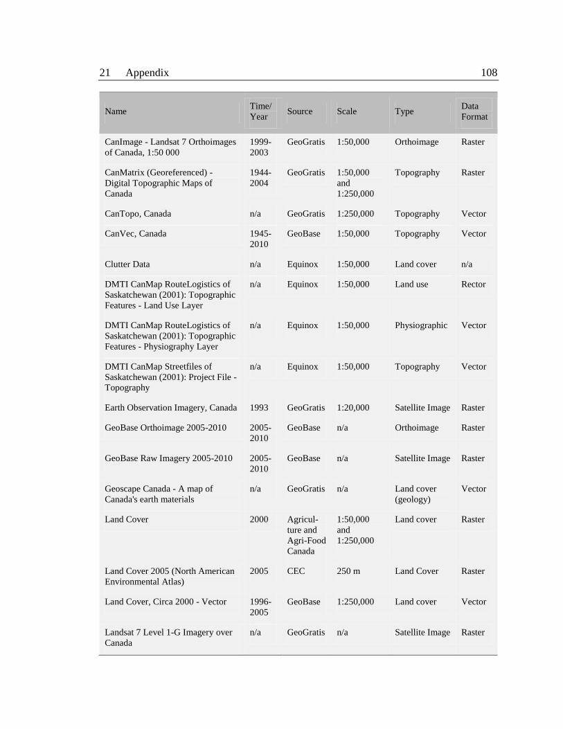
21 Appendix 108

Name Time/


Data

Format

CanImage - Landsat 7 Orthoimages

of Canada, 1:50 000

1999-

2003

GeoGratis 1:50,000 Orthoimage Raster

CanMatrix (Georeferenced) -

Digital Topographic Maps of

Canada

1944-

2004

GeoGratis 1:50,000

and

1:250,000

Topography Raster

CanTopo, Canada n/a GeoGratis 1:250,000 Topography Vector

CanVec, Canada 1945-

2010

GeoBase 1:50,000 Topography Vector

Clutter Data n/a Equinox 1:50,000 Land cover n/a

DMTI CanMap RouteLogistics of

Saskatchewan (2001): Topographic

Features - Land Use Layer

n/a Equinox 1:50,000 Land use Rector

DMTI CanMap RouteLogistics of

Saskatchewan (2001): Topographic

Features - Physiography Layer

n/a Equinox 1:50,000 Physiographic Vector

DMTI CanMap Streetfiles of

Saskatchewan (2001): Project File -

Topography

n/a Equinox 1:50,000 Topography Vector

Earth Observation Imagery, Canada 1993 GeoGratis 1:20,000 Satellite Image Raster

GeoBase Orthoimage 2005-2010 2005-

2010

GeoBase n/a Orthoimage Raster

GeoBase Raw Imagery 2005-2010 2005-

2010

GeoBase n/a Satellite Image Raster

Geoscape Canada - A map of

Canada's earth materials

n/a GeoGratis n/a Land cover

(geology)

Vector

Land Cover 2000 Agricul-

ture and

Agri-Food

Canada

1:50,000

and

1:250,000

Land cover Raster

Land Cover 2005 (North American

Environmental Atlas)

2005 CEC 250 m Land Cover Raster

Land Cover, Circa 2000 - Vector 1996-

2005

GeoBase 1:250,000 Land cover Vector

Landsat 7 Level 1-G Imagery over

Canada

n/a GeoGratis n/a Satellite Image Raster

21 Appendix 109

Name Time/


Data

Format

Landsat 7 Orthorectified Imagery

over Canada

n/a GeoBase n/a Satellite Image Raster

Landsat 7 Orthorectified Imagery

over Canada

n/a GeoGratis n/a Satellite Image Raster

Landsat Image Mosaic of Canada 1990 GeoGratis 1:50,000 Image Mosaic Raster

Multi-Spectral Clear-Sky

Composites of MODIS/Terra Land

Channels (B1-B7) Over Canada at

250m Spatial Resolution and 10-

Day Intervals Since March, 2000:

Top of the Atmosphere (TOA)

Data.

2000-

2006

GeoGratis 1:1,000,000 Satellite Image Raster

RADARSAT Ortho-rectified

Mosaic of Canada, Lambert

Conformal Conic, 250 Metres

1998-

2000

GeoGratis 1:250,000 Satellite Image Raster

SEASAT SAR Data over Canada 1978 GeoGratis n/a Satellite Image Raster

Toporama 1945 GeoGratis 1:50,000 Topography Raster

Toporama Web Map Service n/a NRCan 1:50,000

and

1:250,000

Topography Raster

21 Appendix 110

II. OLS Results

OLS model for LandCover 2005 of the North American Environmental Atlas

Land Cover Class Relationship

Statistically Significant

Coefficients Adjusted

R2

Probability Robust

Probability

Urban and Built-up (18) + yes yes 0.327908

Temperature or sub-polar needle leaf

forest (2) - yes yes 0.001087

Temperature or sub-polar broadleaf

deciduous (6) - yes yes 0.006572

Mixed Forest (7) - no no 0.000005

Temperate or sub-polar shrub land (9) - yes yes 0.003075

Temperature or sub-polar grassland (11) - yes yes 0.010209

Sub-polar or polar barren-lichen-moss

(14) - yes yes 0.000607

Wetland (15) - yes yes 0.000703

Cropland (16) - yes yes 0.314294

Barren Lands (17) + yes yes 0.051175

Water (19) - yes yes 0.003285

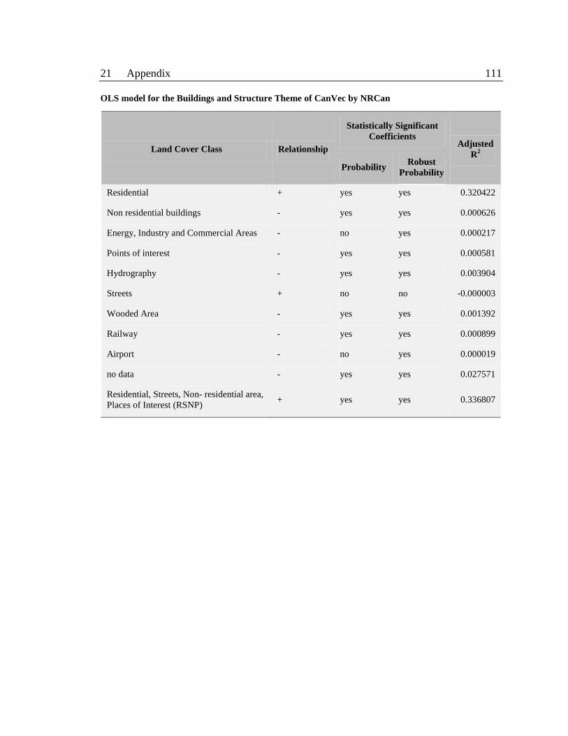
21 Appendix 111

OLS model for the Buildings and Structure Theme of CanVec by NRCan

Land Cover Class Relationship

Statistically Significant

Coefficients Adjusted

R2

Probability Robust

Probability

Residential + yes yes 0.320422

Non residential buildings - yes yes 0.000626

Energy, Industry and Commercial Areas - no yes 0.000217

Points of interest - yes yes 0.000581

Hydrography - yes yes 0.003904

Streets + no no -0.000003

Wooded Area - yes yes 0.001392

Railway - yes yes 0.000899

Airport - no yes 0.000019

no data - yes yes 0.027571

Residential, Streets, Non- residential area,

Places of Interest (RSNP) + yes yes 0.336807

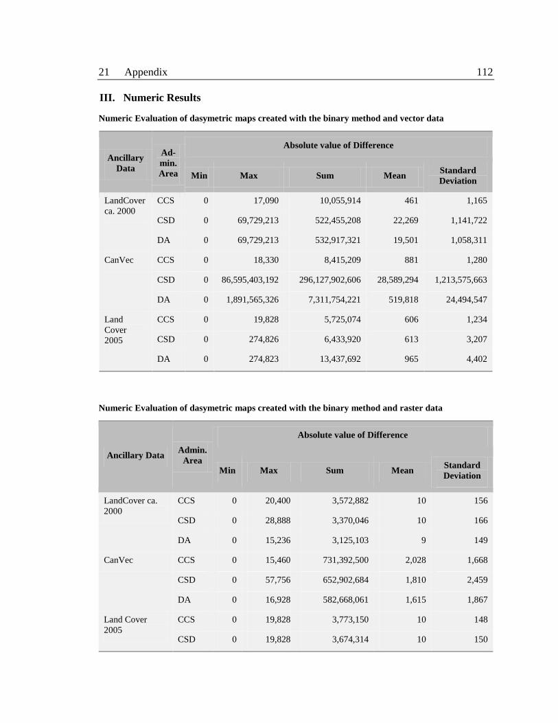
21 Appendix 112

III. Numeric Results

Numeric Evaluation of dasymetric maps created with the binary method and vector data

Ancillary

Data

Ad-

min.

Area

Absolute value of Difference


Deviation

LandCover

ca. 2000

CCS 0 17,090 10,055,914 461 1,165

CSD 0 69,729,213 522,455,208 22,269 1,141,722

DA 0 69,729,213 532,917,321 19,501 1,058,311

CanVec CCS 0 18,330 8,415,209 881 1,280

CSD 0 86,595,403,192 296,127,902,606 28,589,294 1,213,575,663

DA 0 1,891,565,326 7,311,754,221 519,818 24,494,547

Land

Cover

2005

CCS 0 19,828 5,725,074 606 1,234

CSD 0 274,826 6,433,920 613 3,207

DA 0 274,823 13,437,692 965 4,402

Numeric Evaluation of dasymetric maps created with the binary method and raster data

Ancillary Data Admin.

Area



Deviation

LandCover ca.

2000

CCS 0 20,400 3,572,882 10 156

CSD 0 28,888 3,370,046 10 166

DA 0 15,236 3,125,103 9 149

CanVec CCS 0 15,460 731,392,500 2,028 1,668

CSD 0 57,756 652,902,684 1,810 2,459

DA 0 16,928 582,668,061 1,615 1,867

Land Cover

2005

CCS 0 19,828 3,773,150 10 148

CSD 0 19,828 3,674,314 10 150

21 Appendix 113

Ancillary Data Admin.

Area



Deviation

DA 0 19,828 3,428,069 10 152

Street Network

Density

CCS 0 18,221 4,555,146 13 149

CSD 0 18,221 4,406,039 12 148

DA 0 50,655 3,804,583 11 185

Numeric Evaluation of dasymetric maps created with the IDM, the Centroid Method and LandCover

ca. 2000 data

Administrative

Area

Sample

Size



Deviation

CSD 5 0 66,842 12,270,778 584 3,285

20 0 19,828 10,899,649 519 1,572

30 0 17,902 6,193,064 295 838

40 0 17,902 6,193,064 295 838

50 0 17,902 6,193,064 295 838

75 0 17,902 6,193,064 295 838

CCS 5 0 17,747 5,890,175 305 864

10 0 17,747 5,890,175 305 864

15 0 17,747 5,890,175 305 864

20 0 17,946 6,024,956 312 876

50 0 17,946 6,024,956 312 876

21 Appendix 114

Numeric Evaluation of dasymetric maps created with the IDM, the Containment Method and

LandCover ca. 2000 data

Administrative

Area

Sample

Size



Deviation

CSD 5 0 17,902 6,193,064 295 838

20 0 17,902 6,193,064 295 838

30 0 17,902 6,193,064 295 838

40 0 17,902 6,193,064 295 838

50 0 17,902 6,193,064 295 838

75 0 17,902 6,193,064 295 838

CCS 5 0 17,946 6,024,956 312 876

10 0 17,946 6,024,956 312 876

15 0 17,946 6,024,956 312 876

20 0 17,946 6,024,956 312 876

50 0 17,946 6,024,956 312 876

Numeric Evaluation of dasymetric maps created with the IDM, the Percent Coverage Method and


Admin.

Area

Sample

Size Percentage



Deviation

CSD 5 70 0 44,044 6,647,602 317 1,111

80 0 23,106 6,181,835 294 894

90 0 17,902 6,193,064 295 838

100 0 17,902 6,193,064 295 838

20 70 0 17,902 6,193,064 295 838

21 Appendix 115

Admin.

Area

Sample

Size Percentage



Deviation

80 0 17,902 6,193,064 295 838

90 0 17,902 6,193,064 295 838

100 0 17,902 6,193,064 295 838

30 70 0 17,902 6,193,064 295 838

80 0 17,902 6,193,064 295 838

90 0 17,902 6,193,064 295 838

100 0 17,902 6,193,064 295 838

40 70 0 17,902 6,193,064 295 838

80 0 17,902 6,193,064 295 838

90 0 17,902 6,193,064 295 838

100 0 17,902 6,193,064 295 838

50 70 0 17,902 6,193,064 295 838

80 0 17,902 6,193,064 295 838

90 0 17,902 6,193,064 295 838

100 0 17,902 6,193,064 295 838

75 70 0 17,902 6,193,064 295 838

80 0 17,902 6,193,064 295 838

90 0 17,902 6,193,064 295 838

100 0 17,902 6,193,064 295 838

CCS 5 70 0 17,753 5,900,944 306 864

80 0 17,754 5,901,106 306 864

90 0 17,946 6,024,956 312 876

100 0 17,946 6,024,956 312 876

10 70 0 17,753 5,900,944 306 864

21 Appendix 116

Admin.

Area

Sample

Size Percentage



Deviation

80 0 17,946 6,024,956 312 876

90 0 17,946 6,024,956 312 876

100 0 17,946 6,024,956 312 876

15 70 0 17,946 6,024,956 312 876

80 0 17,946 6,024,956 312 876

90 0 17,946 6,024,956 312 876

100 0 17,946 6,024,956 312 876

20 70 0 17,946 6,024,956 312 876

80 0 17,946 6,024,956 312 876

90 0 17,946 6,024,956 312 876

100 0 17,946 6,024,956 312 876

50 70 0 17,946 6,024,956 312 876

80 0 17,946 6,024,956 312 876

90 0 17,946 6,024,956 312 876

100 0 17,946 6,024,956 312 876

Numeric Evaluation of dasymetric map created with the CPDM, Census Subdivisions and



Min Max Sum Mean Standard Deviation

0 2,916,840 981,378,699 2,794 46,355

21 Appendix 117

IV. ArcGIS 10.x Tools

List of ArcGIS 10 tools used to create the dasymetric maps

Tool Path

Buffer Arc Toolbox > Analysis Tools > Proximity > Buffer

Clip (raster) ArcToolbox > Data Management Tools > Raster > Raster Processing > Clip

Create Fishnet ArcToolbox > Data Management Tools > Feature Class > Create Fishnet

Erase Arc Toolbox > Analysis Tools > Overlay > Erase

Feature To Point ArcToolbox > Data Management Tools > Features > Features To Point

Line Density ArcToolbox > Spatial Analyst Tools > Density > Line Density

Ordinary Least

Squares

ArcToolbox > Spatial Statistics Tools > Modeling Spatial Relations > Ordinary

Least Squares

Pivot Table ArcToolbox > Data Management Tools > Table > Pivot Table

Polygon To Raster ArcToolbox > Conversion Tools > To Raster > Polygon To Raster

Spatial

Autocorrelation

(Morans I)

ArcToolbox > Spatial Statistics Tools > Analyzing Patterns > Spatial

Autocorrelation (Morans I)

Spatial Join ArcToolbox > Analysis Tools > Overlay > Spatial Join

Point To Raster ArcToolbox > Conversion Tools > To Raster > Point To Raster

Raster Calculator ArcToolbox > Spatial Analyst Tools > Map Algebra > Raster Calculator

Raster To Point ArcToolbox > Conversion Tools > From Raster > Raster To Point

Union ArcToolbox > Analysis Tools > Overlay > Union

21 Appendix 118

V. Dasymetric Maps of Saskatchewan

Dasymetric Map URL

Saskatchewan’s Population Density

Binary Method (raster)

Resolution: 250 m

Scale: 1:500,000

Note: This map only shows

excerpts for the City of

Regina, the City of

Prince Albert, and Fond

du Lac

www.anne-krahnen.com/DasymetricMapping/

PopulationDensitySaskatchewan_BinaryMethod_250m.jpg



Resolution: 1,125 m

Scale: 1:2,250,000





Resolution: 2,500 m

Scale: 1:5,000,000



22 References 119

22 References

22.1 Literature

ArcGIS Resource Center (2010). On map scale and raster resolution. Retrieved March 5, 2012,

from ArcGIS Blog:

http://blogs.esri.com/esri/arcgis/2010/12/12/on-map-scale-and-raster-resolution/

Bielecka, E. (2005). A dasymetric population density map of Poland. Proceedings of the 22nd

International Cartographic Conference, July 9 - 15, A Coruna, Spain.

Briggs, D., Gulliver, J., Fecht, D. & Vinneau, D. (2007). Dasymetric modelling of small-area

population distribution using land-cover and light emission data. Remote Sensing of

Environment, 108 (4), 451-466.

Crampton, J. W. (2004). GIS and Geographic Governance: Reconstructing the Choropleth Map.

Cartographica, 39 (1), 41 - 53.

de Geer, S. (1926). Review: A Population Density Map of European Russia. Geographical

Review, 16 (2), 341-343.

Dempster, A. P., Laird, N. M. & Rubin, D. B. (1977). Maximum Likelihood Estimation from

Incomplete Data via the EM Algorithm. Journal of the Royal Statistical Societ , 39 (1), 1-38.

Dent, B. D. (1999). Cartography: Thematic Map Design (5 ed.). Boston: McGraw-Hill.

Eicher, C. & Brewer, C. (2001). Dasymetric Mapping and Areal Interpolation: Implementation

and Evaluation. Cartography and Information Science, 28 (2), 125-138.

ESRI (2012.). GIS Dictionary. Retrieved February 01, 2012, from ESRI Support:

http://support.esri.com/en/knowledgebase/Gisdictionary/browse

Fisher, P. F. & Langford, M. (1996). Modeling Sensitivity to Accuracy in Classified Imagery: A

Study of Areal Interpolation by Dasymetric Mapping. Professional Geographer, 48 (3),

299-309.

Flowerdew, R., Green, M. & Kheris, E. (1991). Using Areal Interpolation Methods in Geographic

Information Systems. Papers in Regional Science: The Journal of the RSAI, 70 (3), 303-315.

Gallego, J. & Peedell, S. (2001). Using CORINE Land Cover to map population density.

Towards agri-environmental indicators. EEA Topic report 6/2001, 94-105.

22 References 120

Government of Saskatchewan (2011). Saskatchewan Fact Sheet. Retrieved February 10, 2012,

from Bureau of Statistics:

http://www.stats.gov.sk.ca/Default.aspx?DN=b2e511d6-2c66-4f7d-9461-69f4bffd3629

———. (2010). Bureau of Statistics. Retrieved September 23, 2010, from

http://www.stats.gov.sk.ca/

———. (2007). Saskatchewan Population Report: 2006 Census of Canada. Retrieved September

22, 2010, from Bureau of Statistics:

http://www.stats.gov.sk.ca/stats/pop/Censuspopulation2006.pdf

Gregory, I. (2002). The accuracy of areal interpolation techniques: standardising 19th and 20th

century census data to allow long-term comparison. Computers, Environment and Urban

Systems, 26 (4), 293-314.

Kim, H. & Yao, X. (2010). Pycnophylactic interpolation revisited: integration with the

dasymetric-mapping method. International Journal of Remote Sensing, 31 (21), 5657-5671.

Langford, M. (2007). Rapid faciliation of dasymetric-based population interpolation by means of

raster-pixel maps. Computers, Environment and Urban Systems, 31 (1), 66-80.

———. (2006). Obtaining population estimates in non-census reporting zones: An evaluation of

the 3-class dasymetric method. Computers, Environment and Urban Systems, 30 (2),

161-180.

———. (2003). Refining methods for dasymetric mapping using satellite remote sensing. In V.

Mesev (Ed.), Remotely Sensed Cities (pp. 137-156). London: Taylor & Francis.

Langford, M. & Unwin, D. J. (1994). Generating and mapping population density surfaces within

a geographical information system. The Cartographic Journal, 31, 21 - 26.

Langford, M., Higgs, G., Radcliffe, J. & White, S. (2008). Urban population distribution models

and service accessability estimation. Computers, Environment and Urban Systems, 32 (1),

66-80.

Langford, M., Maguire, D. & Unwin, D. (1991). The areal interpolation problem: estimating

population using remote sensing in a GIS framework. In I. Masser & M. Blakemore (Eds.),

Handling Geographical Information: Methodology and Potential Applications (pp. 55-77).

London: Longman.

Liao, Y., Wang, J., Meng, B. & Li, X. (2008). Integration of GP and GA for mapping population

distribution. International Journal of Geographical Information Science, 1-22.

Maantay, J. & Maroko, A. (2009). Mapping urban risk: Flood hazards, race & environmental

justice in New York. Applied Geography, 29 (1), 111–124.

22 References 121

Maantay, J., Maroko, A. & Hermann, C. (2007). Mapping Population Distribution in the Urban

Environment: The Cadastral-based Expert Dasymetric System. Cartography and

Geographic Information Science, 34 (2), 77-102.

Mayhew, S. (2004). Oxford Dictionary of Geography (3 ed.). New York: Oxford University

Press.

McCleary, G. (1969). The Dasymetric Method in Thematic Cartography. PhD dissertation,

University of Wisconsin.

Mennis, J. (2009). Dasymetric Mapping for Estimating Population in Small Areas. Geography

Compass, 3 (2), 727 - 745.

———. (2003). Generating Surface Models of Population Using Dasymetric Mapping. The

Professional Geographer, 33 (3), 31-42.

Mennis, J. & Hultgren, T. (2006). Intelligent Dasymetric Mapping and Its Application to Areal

Interpolation. Cartography and Geographic Information Science, 33 (3), 179-194.

Monmonier, M. (1996). Ho to Lie with Maps (2 ed.). Chicago: The University of Chicago Press.

Openshaw, S. (1984). The Modifiable Areal Unit Problem. Norwich: GeoBooks.

Petrov, A. N. (2008). Setting the Record Straight: On the Russian Origins of Dasymetric

Mapping. Cartographica, 43 (2), 133 - 136.

Raisz, E. (1962). Principles of Cartography. McGraw-Hill Book Company.

Reibel, M. & Bufalino, M. (2005). Street-weighted interpolation techniques for demographic

count estimation in incompatible zone systems. Environment and Planning A, 37, 127-139.

Robinson, A. (1955). The 1837 Maps of Henry Drury Harness. The Geographical Journal,

121 (4), 440-450.

Schlichtmann, H. (2007). Rural Settlements. In B. Thraves, M. Lewry, J. Dale &

H. Schlichtmann, Saskatchewan: Geographic Perspectives (pp. 271-287). Regina:

Department of Geography, University of Regina, and CPRC.

Scott, L. M. & Janikas, M. V. (2010). Spatial Statistics in ArcGIS. In M. M. Fischer & A. Getis

(Eds.), Handbook of Applied Spatial Analysis: Software Tools, Methods and Applications

(pp. 27-41). Berlin Heidelberg: Springer-Verlag.

Semenov-Tian-Shansky, B. (1928). Russia: Territory and Population: A Perspective on the 1926

Census. Geographical Review, 18 (4), 616-640.

Siegel, J. S. & Swanson, D. A. (Eds.). (2004). The Methods and Materials of Demography

(2 ed.). San Diego/ London: Elsevier Academic Press.

22 References 122

Slocum, T. A., McMaster, R. B., Kessler, F. C. & Howard, H. H. (2009). Thematic Cartography

and Geovisualization (3 ed.). Upper Saddle River: Pearson Prentice Hall.

Statistics Canada. (2010). 2006 Census Dictionary. Retrieved January 31, 2012, from Statistics

Canada:

http://www.statcan.gc.ca/access_acces/alternative_alternatif.action?l=eng&loc=http://www1

2.statcan.gc.ca/census-recensement/2006/ref/dict/pdf/92-566-

eng.pdf&t=2006%20Census%20Dictionary

——— (2007 a). Division No. 6, Saskatchewan (Code4706) (table). Retrieved February 10, 2012,

from 2006 Community Profiles. 2006 Census of Population. Statistics Canada Catalogue no.

92-591-XWE.:

http://www12.statcan.gc.ca/census-recensement/2006/dp-pd/prof/92-591/index.cfm?Lang=E

———. (2007 b). Fond du Lac 227, Saskatchewan (Code4718824) (table). Retrieved March 02,

2012, from 2006 Community Profiles. 2006 Census of Population. Statistics Canada

Catalogue no. 92-591-XWE:

http://census2006.ca/census-recensement/2006/dp-pd/prof/92-591/index.cfm?Lang=E

———. (2007 c). GeoSuite. Statistics Canada Catalogue no. 92-150-XCB, 2006 Census.

———. (2007 d). Prince Albert, Saskatchewan (Code4715066) (table). Retrieved March 02,

2012, from 2006 Community Profiles. 2006 Census of Population. Statistics Canada


http://census2006.ca/census-recensement/2006/dp-pd/prof/92-591/index.cfm?Lang=E

———. (2007 e). Regina, Saskatchewan (Code4706027) (table). Retrieved March 02, 2012, from

2006 Community Profiles. 2006 Census of Population. Statistics Canada Catalogue no. 92-

591-XWE:

http://www12.statcan.gc.ca/census-recensement/2006/dp-pd/prof/92-591/index.cfm?Lang=E

Sykes, A. O. (1993). Regression analysis is a statistical tool for the investigation of relationships.

Chicago Working Paper in Law & Economics .

Thraves, B. (2007). Urban Geography. In B. Thraves, M. Lewry, J. Dale & H. Schlichtmann,

Saskatchewan: Geographic Perspectives (pp. 293-317). Regina: Department of Geography,

University of Regina and CPRC.

Tian, Y., Yue, T., Zhu, L. & Clinton, N. (2005). Modeling population density using land cover

data. Ecological Modeling , 189, 72-88.

Tobler, W. (1979). Smooth pyclophylactic interpolation for geographic regions. Journal of the

American Statistical Association (74), 519-530.

22 References 123

Walford, N. (2011). Practical Statistics for Geographers and Earth Scientists. Wiley-Blackwell.

Wang, X. & Ma, M. (2007). A distance variable to simulate the urban population. In M. Ehlers &

U. Michel (Ed.), Remote Sensing for Environmental Monitoring, GIS Applications, and

Geology VII. Florence, Italy: SPIE.

Willmott, C. J. & Matsuura, K. (2009). Advantages of the mean absolute error (MAE) over the

root mean square error (RMSE) in accessing average model performance. Climate Research,

30, 79-82.

Wright, J. (1936). A Method of Mapping Densities of Population: With Cape Cod as Example.

Geographical Review, 26 (1), 103-110.

22.2 Map data sources

Canada Centre for Remote Sensing (CCRS). (2010). 2005 Land Cover of North America at 250

meters. Retrieved March 1, 2012, from Earth Sciences Sector, Natural Resources Canada:

http://www.cec.org/naatlas/

Government of Canada (2009 a). CanVec, Canada. Retrieved March 1, 2012, from Natural

Resources Canada, Earth Sciences Sector, Centre for Topographic Information:

http://geogratis.ca/geogratis/en/product/search.do?id=5460AA9D-54CD-8349-C95E-

1A4D03172FDF

———. (2009 b). Land Cover, Circa 2000 – Vector. Retrieved March 1, 2012, from Natural

Resources Canada, Earth Sciences Sector, Centre for Topographic Information:

http://geobase.ca/geobase/en/find.do?produit=csc2000v

Statistics Canada. (2007 f). Dissemination Area Boundary File. Retrieved March 1, 2012, from

Statistics Canada Catalogue no. 92-169-XWE:

http://geodepot.statcan.gc.ca/2006/040120011618150421032019/0215211404011825060912

0519/0401-0104_05-eng.jsp

———. (2007 g). Dissemination Blocks Boundary File. Retrieved March 1, 2012, from Statistics

Canada Catalogue no. 92-163-XWE:


0519/0402-0904_05-eng.jsp

———. (2007 h). Urban Area Boundary File. Retrieved March 1, 2012, from Statistics Canada



0519/2101_1821_05-eng.jsp

22 References 124

———. (2006 a). Boundary Files – Cartographic Boundary File - Census Consolidated

Subdivision. Retrieved March 1, 2012, from Statistics Canada Catalogue no. 92-160-XWE:


0519_05-eng.jsp

———. (2006 b). Boundary Files – Cartographic Boundary File – Census Divisions. Retrieved

March 1, 2012, from Statistics Canada Catalogue no. 92-160-XWE:


0519_05-eng.jsp

———. (2006 c). Boundary Files – Cartographic Boundary File - Provinces. Retrieved March 1,

2012, from Statistics Canada Catalogue no. 92-160-XWE:


0519_05-eng.jsp

———. (2006 d). Boundary Files – Water Features –Lakes and Rivers (polygons). Retrieved

March 1, 2012, from Statistics Canada Catalogue no. 92-160-XWE:


0519_05-eng.jsp

———. (2006 e). Census Subdivision Cartographic Boundary File. Retrieved March 1, 2012,

from Statistics Canada Catalogue no. 92-162-XWE:

http://geodepot.statcan.gc.ca/2006/040120011618150421032019/031904_05-eng.jsp

———. (2006 f). Boundary Files – Water Features –Rivers (lines). Retrieved March 1, 2012,

from Statistics Canada Catalogue no. 92-160-XWE:


0519_05-eng.jsp

CARTOGRAPHIC VISUALIZATION OF …ourspace.uregina.ca/bitstream/handle/10294/3630/Krahnen_Anne... ·...

Documents

Transcript of CARTOGRAPHIC VISUALIZATION OF …ourspace.uregina.ca/bitstream/handle/10294/3630/Krahnen_Anne... ·...