Capital Markets and Portfolio Theory (2000)

Capital Markets and PortfolioTheory

Roland PortaitFrom the class notes taken by Peng Cheng

Novembre 2000

Table of Contents

Table of Contents

PART I Standard (One Period) Portfolio Theory . . . . . . . . . . . . . . . . . . . . . 1

1 Portfolio Choices . . . . . . . . . . . . . . . . . . . . . . . . . . . . . . . . . . . . . . . . . . . . . . . . . . . . . . . . 21.A Framework and notations. . . . . . . . . . . . . . . . . . . . . . . . . . . . . . . . . . . . . . . . . . . . . 2

1.A.i No Risk-free Asset . . . . . . . . . . . . . . . . . . . . . . . . . . . . . . . . . . . . . . . . . . . . . . . . 21.A.ii With Risk-free Asset . . . . . . . . . . . . . . . . . . . . . . . . . . . . . . . . . . . . . . . . . . . . . . 4

1.B Efficient portfolio in absence of a risk-free asset . . . . . . . . . . . . . . . . . . . . . . 61.B.i Efficiency criteria . . . . . . . . . . . . . . . . . . . . . . . . . . . . . . . . . . . . . . . . . . . . . . . . . 61.B.ii Efficient portfolio and risk averse investors . . . . . . . . . . . . . . . . . . . . . . . . . . . 81.B.iii Efficient set . . . . . . . . . . . . . . . . . . . . . . . . . . . . . . . . . . . . . . . . . . . . . . . . . . . . . . 91.B.iv Two funds separation (Black) . . . . . . . . . . . . . . . . . . . . . . . . . . . . . . . . . . . . . 10

1.C Efficient portfolio with a risk-free asset . . . . . . . . . . . . . . . . . . . . . . . . . . . . . . 111.D HARA preferences and Cass-Stiglitz 2 fund separation . . . . . . . . . . . . . . 14

1.D.i HARA (Hyperbolic Absolute Risk Aversion) . . . . . . . . . . . . . . . . . . . . . . . . 141.D.ii Cass and Stiglitz separation. . . . . . . . . . . . . . . . . . . . . . . . . . . . . . . . . . . . . . . 15

2 Capital Market Equilibrium . . . . . . . . . . . . . . . . . . . . . . . . . . . . . . . . . . . . . . . . . . 172.A CAPM. . . . . . . . . . . . . . . . . . . . . . . . . . . . . . . . . . . . . . . . . . . . . . . . . . . . . . . . . . . . . . . 17

2.A.i The Model . . . . . . . . . . . . . . . . . . . . . . . . . . . . . . . . . . . . . . . . . . . . . . . . . . . . . 172.A.ii Geometry . . . . . . . . . . . . . . . . . . . . . . . . . . . . . . . . . . . . . . . . . . . . . . . . . . . . . . 192.A.iii CAPM as a Pricing and Equilibrium Model . . . . . . . . . . . . . . . . . . . . . . . . . 192.A.iv Testing the CAPM . . . . . . . . . . . . . . . . . . . . . . . . . . . . . . . . . . . . . . . . . . . . . . 21

2.B Factor Models and APT . . . . . . . . . . . . . . . . . . . . . . . . . . . . . . . . . . . . . . . . . . . . . 212.B.i K-factor models . . . . . . . . . . . . . . . . . . . . . . . . . . . . . . . . . . . . . . . . . . . . . . . . . 212.B.ii APT . . . . . . . . . . . . . . . . . . . . . . . . . . . . . . . . . . . . . . . . . . . . . . . . . . . . . . . . . . . 222.B.iii Arbitrage and Equilibrium . . . . . . . . . . . . . . . . . . . . . . . . . . . . . . . . . . . . . . . . 242.B.iv References . . . . . . . . . . . . . . . . . . . . . . . . . . . . . . . . . . . . . . . . . . . . . . . . . . . . . . 25

PART II Multiperiod Capital Market Theory : theProbabilistic Approach . . . . . . . . . . . . . . . . . . . . . . . . . . . . . . . . . . . . . . . . 26

3 Framework . . . . . . . . . . . . . . . . . . . . . . . . . . . . . . . . . . . . . . . . . . . . . . . . . . . . . . . . . . . . . . 273.A Probability Space and Information . . . . . . . . . . . . . . . . . . . . . . . . . . . . . . . . . . 273.B Asset Prices . . . . . . . . . . . . . . . . . . . . . . . . . . . . . . . . . . . . . . . . . . . . . . . . . . . . . . . . . 28

3.B.i DeÞnitions and Notations. . . . . . . . . . . . . . . . . . . . . . . . . . . . . . . . . . . . . . . . . 283.C Portfolio Strategies . . . . . . . . . . . . . . . . . . . . . . . . . . . . . . . . . . . . . . . . . . . . . . . . . . 29

3.C.i Notation: . . . . . . . . . . . . . . . . . . . . . . . . . . . . . . . . . . . . . . . . . . . . . . . . . . . . . . . 293.C.ii Discrete Time . . . . . . . . . . . . . . . . . . . . . . . . . . . . . . . . . . . . . . . . . . . . . . . . . . . 293.C.iii Continuous Time . . . . . . . . . . . . . . . . . . . . . . . . . . . . . . . . . . . . . . . . . . . . . . . . 30

i

Table of Contents

4 AoA, Attainability and Completeness. . . . . . . . . . . . . . . . . . . . . . . . . . . . . . . 324.A DeÞnitions . . . . . . . . . . . . . . . . . . . . . . . . . . . . . . . . . . . . . . . . . . . . . . . . . . . . . . . . . . . 324.B Propositions on AoA and Completeness . . . . . . . . . . . . . . . . . . . . . . . . . . . . . 35

4.B.i Correspondance between Q and Π : Main Results . . . . . . . . . . . . . . . . . . . 354.B.ii Extensions. . . . . . . . . . . . . . . . . . . . . . . . . . . . . . . . . . . . . . . . . . . . . . . . . . . . . . 38

5 Alternative SpeciÞcations of Asset Prices . . . . . . . . . . . . . . . . . . . . . . . . . . 395.A Ito Process . . . . . . . . . . . . . . . . . . . . . . . . . . . . . . . . . . . . . . . . . . . . . . . . . . . . . . . . . . 395.B Diffusions . . . . . . . . . . . . . . . . . . . . . . . . . . . . . . . . . . . . . . . . . . . . . . . . . . . . . . . . . . . . 405.C Diffusion state variables . . . . . . . . . . . . . . . . . . . . . . . . . . . . . . . . . . . . . . . . . . . . . 41

5.D Theory in the Ito-Diffusion Case . . . . . . . . . . . . . . . . . . . . . . . . . . . . . . . . . . . . 415.D.i Framework . . . . . . . . . . . . . . . . . . . . . . . . . . . . . . . . . . . . . . . . . . . . . . . . . . . . . 415.D.ii Martingales . . . . . . . . . . . . . . . . . . . . . . . . . . . . . . . . . . . . . . . . . . . . . . . . . . . . . 42

5.D.iii Redundancy and Completeness . . . . . . . . . . . . . . . . . . . . . . . . . . . . . . . . . . . . 425.D.iv Criteria for Recognizing a Complete Market . . . . . . . . . . . . . . . . . . . . . . . . 44

PART III State Variables Models: the PDE Approach. . . . . . . . . . . . . . . . 45

6 Framework . . . . . . . . . . . . . . . . . . . . . . . . . . . . . . . . . . . . . . . . . . . . . . . . . . . . . . . . . . . . . . 46

7 Discounting Under Uncertainty . . . . . . . . . . . . . . . . . . . . . . . . . . . . . . . . . . . . . . 487.A Itos lemma and the Dynkin Operator . . . . . . . . . . . . . . . . . . . . . . . . . . . . . . . 487.B The Feynman-Kac Theorem . . . . . . . . . . . . . . . . . . . . . . . . . . . . . . . . . . . . . . . . . 48

8 The PDE Approach . . . . . . . . . . . . . . . . . . . . . . . . . . . . . . . . . . . . . . . . . . . . . . . . . . . 508.A Continuous Time APT . . . . . . . . . . . . . . . . . . . . . . . . . . . . . . . . . . . . . . . . . . . . . . 50

8.A.i Alternative decompositions of a return . . . . . . . . . . . . . . . . . . . . . . . . . . . . . 508.A.ii The APT Model (continuous time version). . . . . . . . . . . . . . . . . . . . . . . . . . 51

8.B One Factor Interest Rate Models . . . . . . . . . . . . . . . . . . . . . . . . . . . . . . . . . . . . 538.C Discounting Under Uncertainty. . . . . . . . . . . . . . . . . . . . . . . . . . . . . . . . . . . . . . 53

9 Links Between Probabilistic and PDE Approaches . . . . . . . . . . . . . . . 559.A Probability Changes and the Radon-Nikodym Derivative . . . . . . . . . . . 559.B Girsanov Theorem . . . . . . . . . . . . . . . . . . . . . . . . . . . . . . . . . . . . . . . . . . . . . . . . . . . 569.C Risk Adjusted Drifts: Application of Girsanov Theorem . . . . . . . . . . . . 56

PART IV The Numeraire Approach . . . . . . . . . . . . . . . . . . . . . . . . . . . . . . . . . . . . . 59

10 Introduction . . . . . . . . . . . . . . . . . . . . . . . . . . . . . . . . . . . . . . . . . . . . . . . . . . . . . . . . . . . . 60

11 Numeraire and Probability Changes . . . . . . . . . . . . . . . . . . . . . . . . . . . . . . . . 6111.AFramework . . . . . . . . . . . . . . . . . . . . . . . . . . . . . . . . . . . . . . . . . . . . . . . . . . . . . . . . . . 61

11.A.i Assets . . . . . . . . . . . . . . . . . . . . . . . . . . . . . . . . . . . . . . . . . . . . . . . . . . . . . . . . . 61

ii

Table of Contents

11.A.ii Numeraires . . . . . . . . . . . . . . . . . . . . . . . . . . . . . . . . . . . . . . . . . . . . . . . . . . . . . 6111.BCorrespondence Between Numeraires and Martingale Probabilities . 62

11.B.i Numeraire → Martingale Probabilities . . . . . . . . . . . . . . . . . . . . . . . . . . . . . 6211.B.ii Probability → Numeraire . . . . . . . . . . . . . . . . . . . . . . . . . . . . . . . . . . . . . . . . . 63

11.CSummary . . . . . . . . . . . . . . . . . . . . . . . . . . . . . . . . . . . . . . . . . . . . . . . . . . . . . . . . . . . . 63

12 The Numeraire (Growth Optimal) Portfolio . . . . . . . . . . . . . . . . . . . . . . . 6512.ADeÞnition and Characterization . . . . . . . . . . . . . . . . . . . . . . . . . . . . . . . . . . . . . 65

12.A.i DeÞnition of the Numeraire (h,H) . . . . . . . . . . . . . . . . . . . . . . . . . . . . . . . . . 6512.A.ii Characterization and Composition of (h,H) . . . . . . . . . . . . . . . . . . . . . . . . 6512.A.iii The Numeraire Portfolio and Radon-Nikodym Derivatives . . . . . . . . . . . . 69

12.BFirst Applications . . . . . . . . . . . . . . . . . . . . . . . . . . . . . . . . . . . . . . . . . . . . . . . . . . . 6912.B.i CAPM . . . . . . . . . . . . . . . . . . . . . . . . . . . . . . . . . . . . . . . . . . . . . . . . . . . . . . . . . 7012.B.ii Valuation. . . . . . . . . . . . . . . . . . . . . . . . . . . . . . . . . . . . . . . . . . . . . . . . . . . . . . . 70

PART V Continuous Time Portfolio Optimization. . . . . . . . . . . . . . . . . . . . 72

13 Dynamic Consumption and Portfolio Choices (The MertonModel) . . . . . . . . . . . . . . . . . . . . . . . . . . . . . . . . . . . . . . . . . . . . . . . . . . . . . . . . . . . . . . . . . . 7313.AFramework . . . . . . . . . . . . . . . . . . . . . . . . . . . . . . . . . . . . . . . . . . . . . . . . . . . . . . . . . . 73

13.A.i The Capital Market . . . . . . . . . . . . . . . . . . . . . . . . . . . . . . . . . . . . . . . . . . . . . 7313.A.ii The Investors (Consumers) Problem . . . . . . . . . . . . . . . . . . . . . . . . . . . . . . . 74

13.BThe Solution. . . . . . . . . . . . . . . . . . . . . . . . . . . . . . . . . . . . . . . . . . . . . . . . . . . . . . . . . 7413.B.i Sketch of the Method . . . . . . . . . . . . . . . . . . . . . . . . . . . . . . . . . . . . . . . . . . . . 7413.B.ii Optimal portfolios and L+ 2 funds separation . . . . . . . . . . . . . . . . . . . . . . 7713.B.iii Intertemporal CAPM . . . . . . . . . . . . . . . . . . . . . . . . . . . . . . . . . . . . . . . . . . . . 78

14 THE EQUIVALENT STATIC PROBLEM (Cox-Huang,Karatzas approach) . . . . . . . . . . . . . . . . . . . . . . . . . . . . . . . . . . . . . . . . . . . . . . . . . . . . 8014.ATransforming the dynamic into a static problem . . . . . . . . . . . . . . . . . . . . 80

14.A.i The pure portfolio problem . . . . . . . . . . . . . . . . . . . . . . . . . . . . . . . . . . . . . . . 8014.A.ii The consumption-portfolio problem . . . . . . . . . . . . . . . . . . . . . . . . . . . . . . . . 82

14.BThe solution in the case of complete markets . . . . . . . . . . . . . . . . . . . . . . . . 8314.B.i Solution of the pure portfolio problem . . . . . . . . . . . . . . . . . . . . . . . . . . . . . 8314.B.ii Examples of speciÞc utility functions . . . . . . . . . . . . . . . . . . . . . . . . . . . . . . . 8514.B.iii Solution of the consumption-portfolio problem . . . . . . . . . . . . . . . . . . . . . . 8614.B.iv General method for obtaining the optimal strategy x∗∗ . . . . . . . . . . . . . . . 87

14.CEquilibrium: the consumption based CAPM . . . . . . . . . . . . . . . . . . . . . . . . 88

PART VI STRATEGIC ASSET ALLOCATION . . . . . . . . . . . . . . . . . . . . . . . 90

15 The problems . . . . . . . . . . . . . . . . . . . . . . . . . . . . . . . . . . . . . . . . . . . . . . . . . . . . . . . . . . . 91

16 The optimal terminal wealth in the CRRA, mean-variance

iii

Table of Contents

and HARA cases . . . . . . . . . . . . . . . . . . . . . . . . . . . . . . . . . . . . . . . . . . . . . . . . . . . . . . . 9216.A Optimal wealth and strong 2 fund separation. . . . . . . . . . . . . . . . . . . . . . . 9216.B The minimum norm return . . . . . . . . . . . . . . . . . . . . . . . . . . . . . . . . . . . . . . . . . 92

17 Optimal dynamic strategies for HARA utilities in two cases . . . . 9317.A The GBM case. . . . . . . . . . . . . . . . . . . . . . . . . . . . . . . . . . . . . . . . . . . . . . . . . . . . . . 9317.B Vasicek stochastic rates with stock trading . . . . . . . . . . . . . . . . . . . . . . . . . 93

18 Assessing the theoretical grounds of the popular advice . . . . . . . . . 9418.AThe bond/stock allocation puzzle . . . . . . . . . . . . . . . . . . . . . . . . . . . . . . . . . . . 9418.BThe conventional wisdom . . . . . . . . . . . . . . . . . . . . . . . . . . . . . . . . . . . . . . . . . . . . 94

REFERENCES 95

iv

PART I

Standard (One Period)Portfolio Theory

Chapter 1 Portfolio Choices

Chapter 1Portfolio Choices

1.A Framework and notations

In all the following we consider a single period or time interval (0 1), hence twoinstants t = 0 and t = 1Consider an asset whose price is S(t) (no dividends or dividends reinvested).

The return of this asset between two points in time (t = 0, 1) is:

R =S (1)− S (0)

S (0)

We now consider the case of a portfolio. and distinguish the case where ariskless asset does not exist from the case where a risk free asset is traded.

1.A.i No Risk-free Asset

There are N tradable risky assets noted i = 1, ..., N :

The price of asset i is Si(t), t = 0, 1.

The return of asset i is

Ri =Si (1)− Si (0)

Si (0)

2


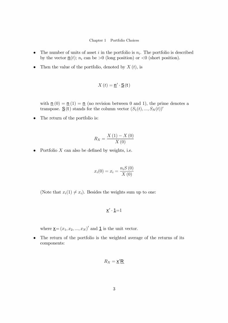
The number of units of asset i in the portfolio is ni. The portfolio is describedby the vector n(t); ni can be >0 (long position) or <0 (short position).

Then the value of the portfolio, denoted by X (t), is

X (t) = n0 · S (t)

with n (0) = n (1) = n (no revision between 0 and 1), the prime denotes atranspose. S (t) stands for the column vector (S1(t), ..., SN(t))0

The return of the portfolio is:

RX =X (1)−X (0)

X (0)

Portfolio X can also be deÞned by weights, i.e.

xi(0) = xi =niS (0)

X (0)

(Note that xi(1) 6= xi). Besides the weights sum up to one:

x0 · 1=1

where x=(x1, x2, ..., xN)0 and 1 is the unit vector.

The return of the portfolio is the weighted average of the returns of itscomponents:

RX = x0R

3


Proof

1+RX =X (1)

X (0)

=n0S (1)X (0)

=NXi=1

niSi (1)

X (0)· Si (0)Si (0)

=NXi=1

xi · Si (1)Si (0)

=NXi=1

xi · (1+Ri)

= 1+NXi=1

xiRi

Q.E.D.

DeÞne µi = E [Ri] and µ=(µ1, µ2, ..., µN)0, then:

µX = E (RX) = x0µ

Denote the variance-covariance matrix of returns ΓN×N = (σij), whereσij = cov (Ri, Rj), then:

var (RX) = var (x0R)= x0Γx

=NXi=1

NXj=1

xixjσij

1.A.ii With Risk-free Asset

We now have N+1 assets, with asset 0 being the risk-free asset, and the remainingN assets being the risky assets.

4


S0 (1) = S0 (0) · (1 + r) with r a deterministic interest rate. Again we can deÞne the portfolio in units, with n=(n0, n1, n2, ..., nN)

0

The portfolio can be similarly deÞned in weights:

xi =niS (0)

X (0)

for the N risky assets (i = 1, 2, ...,N), and

x0 = 1−NXi=1

xi

Note that now

x0 · 1 6= 1where x=(x1, x2, ..., xN)

0 denotes the weights in the N risky assets.

The return of the portfolio is:

RX = x0r +NXi=1

xiRi = r +NXi=1

xi (Ri − r)

The term (Ri − r) is the excess return of asset i over r. Moreover:µX = E (RX) = r + x0π

where π is the risk premium vector of the E (Ri − r) Also denote ΓN×N as the variance-covariance matrix of the risky assets, then:

var (RX) = x0Γx

Γ is always positive semi-deÞnite (meaning that ∀x, x0Γx ≥ 0). In some casesit is positive deÞnite (∀x 6= 0, x0Γx > 0).

DeÞnition 1 Assets i = 1, 2, ..., N are redundant if there exist N scalars λ1,λ2, ...,λN suchthat

PNi=1 λiRi = k, where k is a constant. Then the portfolio λ is risk-free.

Proposition 1The N assets i = 1, 2, ..., N are not redundant iff Γ is positive deÞnite (i.e. non-singular or invertible).

5


Proof

Assume that the assets are redundant, then there exist N scalars λ1,λ2, ...,λN such thatPNi=1 λiRi = k. Consider the portfolio deÞned by the weights λ. The variance of its return =

var (k) = 0 = λ0Γλ, i.e. Γ is singular and not positive deÞnite. Conversely if Γ is singularand not positive deÞnite there exist a non 0 vector λ such that λ0Γλ = 0; Then the return ofportfolio λ has zero variance and

PNi=1 λiRi = k

Q.E.D.

Remark 1 In the following sections we will assume that the assets are non-redundant (it isalways possible to drop redundant assets if any).

1.B Efficient portfolio in absence of a risk-free asset

1.B.i Efficiency criteria

DeÞnition 2 Portfolio (x∗,X∗) is efficient if ∀y, σY < σX∗ ⇒ µY < µX∗ and σY =σX∗ ⇒ µY ≤ µX∗

Consider any efficient portfolio (x∗, X∗) and let variance(RX) = kx∗ solves the optimization program (P ) :

maxxE [RX ] s.t. x0Γx = k ; x01 = 1

The Lagrangian is:

Lµ

x,θ

2,λ

¶= x0µ− θ

2x0Γx− λx01

The Þrst order condition¡∂L∂x= 0

¢writes:

µ− θΓx∗−λ1 = 0

or equivalently, for i = 1, .., N :

µi = λ+ θNXj=1

x∗jσij

6


Remark that these Þrst order conditions are necessary and also sufficient for thesolution being a maximum since the second order conditions hold (L(x) is strictlyconcave -Γ positive deÞnite).

Theorem 1A portfolio (x,X) is efficient iff there exist two scalars λ and θ such that for alli = 1, 2, ..., N:

µi = λ+ θ · cov (Rx, Ri)

Proof

The necessary and sufficient condition for x to be efficient is that it satisÞes the Þrst ordercondition: for all i: µi = λ+ θ

PNj=1 x

∗jσij. We then have:

µi = λ+ θNXj=1

x∗jcov (Ri, Rj)

= λ+ θ · covRi, NX

j=1

x∗jRj

= λ+ θcov (Ri, RX)

Q.E.D.

Remark 2 The second term can be considered as the additional required rate of return (riskpremium), proportional to cov (Ri, RX).

Remark 3 If cov (Ri, RX) = 0, then µi = λ.

Remark 4 Also note:

var (RX) =NXi=1

NXj=1

xixjσij

=NXi=1

xi · covRi, NX

j=1

xjRj

=

NXi=1

xi · cov (Ri, RX)

The covariance term cov (Ri, RX) indicates the contribution of asset i to the total risk of theportfolio. Therefore, additional required rate of return should be proportional to this induced riskwhich is what is stated in the theorem. Moreover cov (Ri, RX) appears to be the relevant measureof risk for any asset i embedded in the portfolio X.

7


1.B.ii Efficient portfolio and risk averse investors

DeÞne another optimization program (P 0), equivalent to (P ) :

(P 0) max

µx0µ−θ

2x0Γx

¶s.t. : x01 = 1

( (P ) and (P 0) yield the same solutions since they have the same Lagrangian)(P 0) writes, equivalently:

Max E [RX ]−θ2var (RX) , s.t. : x01 = 1

In (P 0) θ is interpreted as a given risk-aversion while in (P ) it is an unknownlagrangian multiplier.In (P ) we are given σ2X and we solve for θ and λ as functions of σ

2X . In (P

0) weare given the risk-aversion parameter θ and solve for σ2X as function of θ.

The Þrst order conditions of (P) write as for (P): µ− θΓx∗−λ1 = 0 (with onlyone multiplier for (P 0))

Consider the case of minimum variance portfolio where θ =∞, i.e.

min1

2x0Γx s.t. : x01 = 1

The Lagrangian is then:

L (x,λ) = 1

2x0Γx− λx01

Call k1 the solution. The Þrst order condition gives:

Γk1 − λ1 = 0

Together with the constraint k011 = 1 gives:

λ =1

10Γ−11

Thus:

k1 = λΓ−11

=1

10Γ−11· Γ−11

8


1.B.iii Efficient set

DeÞnition 3 The Efficient Set is the set of all x∗ that obey the Þrst order condition. Equiv-alently, it is the set of all x∗ that solve the optimization program (P 0) ∀θ ≥ 0.

Recall that the Þrst order condition for (P 0) is:

µ− θΓx∗−λ1 = 0

DeÞne risk tolerance bθ as the inverse of risk aversion, i.e.bθ = 1

θ

Then x∗ can be solved as:

x∗ = bθΓ−1 ¡µ− λ1¢

To Þnd λ, use the constraint 10x∗ = 1, i.e.

1 = 10x∗

= 10 · bθΓ−1 ¡µ− λ1¢

Then: bθ10Γ−1µ− bθλ10Γ−11 = 1

or: bθ10Γ−1µ− bθλ10Γ−11 = bθθThis solves for λ:

λ =10Γ−1µ−θ

10Γ−11

Then:

x∗ = bθΓ−1 ¡µ− λ1¢

= bθΓ−1µµ− 10Γ−1µ− θ10Γ−11

·1¶

=Γ−11

10Γ−11+ bθΓ−1µµ− 10Γ−1µ

10Γ−11·1¶

9


We recognize in the Þrst term the minimum variance portfolio (k1) and we callk2 the second term:

k1 =Γ−11

10Γ−11

k2 = Γ−1·µ− 10Γ−1µ

10Γ−11·1¸

Then the solution of (P ) writes:

x∗ = k1 +bθk2

Note that k011 = 1 and x∗01 = 1, therefore k021 = 0. Any efficient portfolio is thusthe sum of k1 (the minimum variance portfolio) and k2 which is a zero weight(zero investment) portfolio. As it could be expected, an investor with a zero risktolerance will hold only k1; If he has a positive risk tolerance bθ he will add a risktaking the form bθk2 in order to increase the expected return. The efficient set cannow be caracterized as:

ES =n

x∗|x∗ = k1 +bθk2 ∀bθ > 0o

Since the expected return x∗0µ is linear in bθ and the variance is quadratic in bθ, inthe (σ2, R) space the efficient portfolios are represented by the efficient frontier,which is a parabola. Each point on the efficient frontier corresponds to a given θ,the slope of the parabola at this point being equal to θ

2(the shadow price in (P )

of the constraint on variance).

In the (σ, R) space the efficient frontier is an hyperbola.

1.B.iv Two funds separation (Black)

Theorem 2Consider any two efficient portfolio x and y:

1. Any convex combination of x and y is efficient, i.e.∀ u ∈ [0, 1] , ux+(1− u)y ∈ES

2. Any efficient portfolio is a combination of x and y (not necessarily a convexcombination)

3. The whole parabola (efficient and inefficient frontier) is generated by (all)combinations of x and y

10


Proof

Since x∈ ES and y∈ ES, for some positive bθX andbθY , we have:x = k1 +

bθXk2

y = k1 +bθY k2

Let z = ux+ (1− u)y, then:

z = [uk1 + (1− u)k1] +hubθX + (1− u)bθY ik2

= k1 +bθZk2

With bθZ > 0, we can conclude that z∈ ES. Let z∈ ES, then z = k1 +

bθZk2 for some bθZ > 0. For any x∈ ES andy∈ ES:

ux+ (1− u)y = k1 +hubθX + (1− u)bθY ik2

By equating bθZ to ubθX + (1− u)bθY we get:u∗ =

bθZ − bθYbθX − bθYThen the combination u∗x+ (1− u∗)y = z

Q.E.D.

1.C Efficient portfolio with a risk-free asset

Consider Þgure 1 where the upper branch of the hyperbola EFR represents, in the(σ, E) space, the efficient portfolios in absence of a riskless asset. Assume now thatexists a risk free asset 0 yielding the certain return r. M stands for the tangencypoint of the hyperbola EFR with a straight line drown from r representing asset 0.Point M represents a portfolio composed only of risky assets, called the tangentportfolio.

11


• Efficient frontier in presence of a riskless assetσ

E

r

MX

EFR

Figure 1.1.

12


Proposition 21. Asset 0 is efficient

2. Consider any portfolio X. Any combination of 0 and X yieldingR = uRX +(1− u) r, lies on the straight line connecting 0 and X in the (σ, E)space

3. Any feasible portfolio which representative point is not on r −M (such as X)is dominated by portfolios in r −M. The straight line r −M is the efficientfrontier and is called the Capital Market Line

4. (Tobins Two-fund Separation) Any efficient portfolio is a combination of anytwo efficient portfolios, for instance 0 and M

5. Any efficient portfolio writes:

x∗ = bθΓ−1 ¡µ−r1¢6. The tangent portfolio (m,M) is:

m = bθMΓ−1 ¡µ−r1¢bθM =1

10Γ−1¡µ−r1¢

Proof

1, 2, 3, 4 are standard and easy to prove. Let us proove 5 and 6: x∗ ∈ ES solves:

max 1r + x∗0¡µ− r1¢− θ

2x∗0Γx∗

The Þrst order condition is:

µ− r1 = θΓx∗

Then:

x∗ =1

θΓ−1

¡µ− r1¢

= bθΓ−1¡µ− r1¢

The tangent portfolio is an efficient portfolio, therefore, m= bθMΓ−1¡µ− r1¢. Also: m01 = 1,

then:

bθM =1

10Γ−1¡µ− r1¢

Q.E.D.

13


Remark 5 Given a risk tolerance bθ: bθ < bθM , the portfolio is long in 0 and m

bθ > bθM , the portfolio shorts 0Remark 6 We deÞne later the market portfolio as a portfolio containing all the risky assetspresent in the market (and only risky assets). In absence of riskless asset the market portfolio isefficient iif its representative point belongs to the hyperbola EFR. In presence of a risk free assetthe necessary and sufficient condition for the market portfolio to be efficient is that it coincideswith the tangent portfolio m (which is the only efficient portfolio of EFR, in presence of a riskfree asset). Would all investors face the same efficient frontier (it would be the case underhomogeneous expectations and horizon) and would they all follow the mean-variance criteria,they would all hold combinations of 0 and M and the tangent portfolio M would necessarilycoincide with the market portfolio.

1.D HARA preferences and Cass-Stiglitz 2 fund separation

A rational agent (in the sense of Von Neumann-Morgenstern) should maximizethe expected utility of wealth E [U (W )].

1.D.i HARA (Hyperbolic Absolute Risk Aversion)

A utility function U (W ) belongs to HARA class if it writes:

U (W ) =γ

1− γ·bθ + W

γ

¸1−γSome restrictions are imposed on the coefficients γ and bθ and the domain ofdeÞnition.

The absolute risk tolerance (ART) and absolute risk aversion (ARA) are:

ART =1

ARA

= −U0

U 00

= bθ + Wγ

14


and the relative risk tolerance (RRT) is:

RRT =bθW+1

γ

In particular:

1. bθ = 0⇒U (W ) =

W 1−γ

1− γWe obtain CRRA, i.e. constant relative risk aversion.A limit case of CRRA is obtained for γ = 1 which can be showed to beequivalent to the Log utility

2. γ = −1⇒

U (W ) =W − W2

2bθi.e. the quadratic utility function.

3. Using a quadratic utility function implies a mean-variance criteria; Indeed:

min var (RX) s.t. E [RX ] = bE (and x01 = 1)⇔ minE [R2X ] s.t. E [RX ] = bE (and x01 = 1)

⇔ minE [X2 (1)] s.t. E [X (1)] = X (0) ·h1 + bEi

⇔ minE[X2 (1)]− λE [X (1)]⇔ maxE

£X (1)− 1

λX2 (1)

¤4. Three undesirable features of the quadratic utility:

Saturation at W = bθ (for that wealth U (W ) =W − W2

2bθ is maximum; U (W ) decreases

for W > bθ!) ARA increasing with wealth (it is commonly admitted that ARA decreases for most

agents).

Indifference to skewness (only the two Þrst moments of W matter), whereas mostinvestors actually like skewness.

1.D.ii Cass and Stiglitz separation

Cass and Stiglitz showed that all HARA investors sharing the same exponential

15


parameter γ can build their optimal portfolios by mixing the two same funds.When a risk free asset exists it can be chosen as one of the two funds. Since allquadratic (mean-variance) investors exhibit the same γ(= −1) Tobin and Black2 fund separation are particular cases of Cass and Stiglitz separation. Cass andStiglitz conditions on the utility functions for separation to hold for investorssharing the same exponential parameter are summarized in the following table

Complete Market Incomplete Market@r (under complete markets ∃ r) quadratic or CRRA2

∃ r class wider than HARA HARA

2 in the particular case of CRRA one fund suffices (for a given γ the portfolio is the same for all W

16

Chapter 2 Capital Market Equilibrium

Chapter 2Capital Market Equilibrium

2.A CAPM

2.A.i The Model

Consider again N risky assets (a risk free asset may exist or not). The marketvalue of asset i is Vi, then (by deÞnition of the market portfolio) its weight in themarket portfolio is:

mi =ViPNi=1 Vi

The return of the market portfolio is:

RM = m0R

Hypothesis 1 (H) : The market portfolio M is efficient.

Remark 7 The market portfolio would be efficient if all investors would hold efficient port-folios (since a combination of efficient portfolios is efficient).

Theorem 3(General CAPM )

1. If (H) is true, then there exist θ and λ such that, for i = 1, ..., N :

µi = E [Ri]

= λ+ θcov (RM , Ri)

2. Conversely, if there exist θ and λ such that, for i = 1, ..., N : µi =λ+ θcov (RM , Ri), then (H) is true.

17


Proof

The proof comes directly from Theorem 1.

Q.E.D.

Remark 8 θ can be interpreted as the risk aversion of the average (representative) investor.

Remark 9 CAPM holds for any portfolio (x,X).

Indeed, call RX its return and consider the case where no risk free asset exists(x01 = 1) :

E [RX ] =NXi=1

xiµi

=NXi=1

xi (λ+ θcov (RM , Ri))

=NXi=1

xiλ+ θNXi=1

xicov (RM , Ri)

= λ+ θcov

ÃRM ,

NXi=1

xiRi

!= λ+ θcov (RM , RX)

Remark 10 The proof follows the same lines when the portfolio contains a risk free assetwith weight x0

Remark 11 λ and θ are the same for all assets or portfolios

Remark 12 For the market portfolio:

µM = λ+ θcov (RM , RM)

= λ+ θσ2M

Therefore:

θ =µM − λσ2M

Then:

µi = λ+ θcov (RM , Ri)

= λ+

·µM − λσ2M

¸cov (RM , Ri)

18


DeÞne:

βi =cov (RM , Ri)

σ2M

Then we may write the CAPM equation in the alternative form:

E [Ri] = λ+ βi (µM − λ)

Consider any portfolio z with βZ = 0:

βZ = 0

⇔ cov (RM , RZ) = 0

⇔ cov (m0R, z0R) = z0Γm = 0

⇐⇒ z ⊥Γm

⇔ z ∈ [vect (Γm)]⊥

vect [v1,v2, ...,vN ] is the set of all linear combinations of v1,v2, ...,vN , or linearsubspace generated by v1,v2, ...,vN . The dimension of [vect (Γm)]⊥ is thus N−1and there are an inÞnity of 0-beta portfolios. Now, from the general CAPM, wewould have: λ = µZ ; Thus:

Corollary 1 (0−beta CAPM) IfM is efficient, for any zero beta portfolio or asset Z: E [Ri] =µZ + βi (µM − µZ)

Corollary 2 (Standard CAPM) : If there exists a risk-free asset yielding r (which is a par-ticular zero beta asset)

E [Ri] = r + βi (µM − r)Note that µZ = r for any zero beta portfolio or asset.

2.A.ii Geometry

missing

2.A.iii CAPM as a Pricing and Equilibrium Model

For a security delivering eV (1) at time 1(the pdf of eV (1) is given, thusE(eV (1)) and cov(eV (1) , RM) are known), what is its price V (0) at time 0?

19


Lets assume that there exists a risk-free asset, then:

EheV (1)iV (0)

= E [1 +R] = 1 + r + θcov

Ã eV (1)V (0)

, RM

!

with

θ =µM − rσ2M

Then:

EheV (1)i = (1 + r)V (0) + θcov ³eV (1) , RM´

and

V (0) =EheV (1)i− θcov ³eV (1) , RM´

1 + r

i.e. V (0) is the present value of its certainty equivalent at time 1 discountedat the risk-free rate.However this asset may be an element of the market portfolio M (unless thisclaim is in zero net supply ..) and therefore the previous pricing formula isnot a closed form general equilibrium relation.

In fact CAPM is an equilibrium condition stemming from the demand side;The equilibrium price can only be otained by specifying the supply side (inthe previous example the supply was a right on an exogeneous cash ßow X).General equilibrium requires a speciÞcation of the supply of all securitiestraded in the market.

Consider the N risky assets together and we look for their equilibrium prices. Weassume Þrst an inelastic supply. Assume that asset i delivers eVi (1), an exogenous cashßow, at time 1, what is its price at time 0?

EheVi (1)iVi (0)

= 1+ r +

·µM − rσ2M

¸cov

Ã eVi (1)Vi (0)

, RM

!

For i = 1, 2, ..., N . We have N equations with N unknowns Vi (0) (i = 1, ..., N).

(1+RM =PN

i=1eVi(1)PN

i=1 Vi(0)allows to compute µM , σ

2M , cov

³ eVi(1)Vi(0) , RM

´as functions of the

Vi (0))

Consider again the N risky assets and an elastic supply with constant returns to scale,where the joint pdf of the Ri is given and independent of the scale Vi(0) to be investedin technology i. The CAPM determines the scale Vi (0) of investment in technology i

20


by the equations:

µi = E [Ri] = r +

·µM − rσ2M

¸cov (RM , Ri)

and

1+RM =

PNi=1 Vi (0) · (1+Ri)PN

i=1 Vi (0)

2.A.iv Testing the CAPM

One remark about this important empirical topic.Testing the CAPM is equivalent to testing (H). However, how should we deÞnethe market portfolio and how to measure the market return?Usually the market portfolio is proxied by stock (plus bond) indices. But resultson stock indices do not include all assets inM (non tradable assets, art,..). Hencewe test the efficiency of the index and not that of M (Rolls Critique).

2.B Factor Models and APT

2.B.i K-factor models

Hypothesis 2 There exist K factors, Fk, k = 1, 2, ...K with

1. Fi ⊥ Fj2. E [Fk] = 0

3. var (Fk) = σ2k

such that for i = 1, 2, ..., N :

Ri = µi +KXk=1

βikFk + ²i

where E [²i] = 0 and ²i ⊥ ²j ⊥ Fk. In vector form:

RN×1 = µ+ βN×KFK×1 + ² = µ+KXk=1

β0kFk + ²

21


with βk being the kth row of β.

In practice, we should have large N and small K, so that in estimating thevariance-covariance matrix,

cov (Ri, Rj) =KXk=1

βikβjkσ2k

we only need to estimate K terms of σ2k and run N regressions for estimatingthe βik.

In CAPM or in the Markowitz model, without the factor decomposition, weneed to estimate N (N − 1) /2 terms.

A Particular case: K = 1 boils down into the market model that writes:

Ri = µi + βiF + ²i

Then:

RM =NXi=1

miµi + FNXi=1

miβi +NXi=1

mi²i

= µM + F

Since the innovation terms diversify and βM =PN

i=1miβi = 1:

F = RM − µMand

Ri = µi + βi [RM − µM ] + ²i

Note that the Ri are linked through [RM − µM ] (since cov (Ri, Rj) = βiβjσ2M).

Also, βi [RM − µM ] is the systematic risk, and ²i is the unsystematic (diversiÞable)risk; only systematic risk should be priced (CAPM).

2.B.ii APT

We assume that the returns are generated by a K factors linear process previouslydeÞned that writes:

22


R = µ++βF+ ² = µ+KXk=1

βkFk + ²

Recall that βkis an N dimensioned column vector with an ith component equal

to βik

DeÞnition 4 A zero investment portfolio, deÞned by the amount of wealth, x, invested ineach asset, satisÞes:

x01 = 0

V (0) = 0

V (1) = x0R

The last equation can be veriÞed since:

V (1) =NXi=1

xi (1 +Ri) =NXi=1

xi +NXi=1

xiRi = x0R

DeÞnition 5 An arbitrage portfolio is a zero investment portfolio with x0R ≥ 0 almostsurely and E [x0R] > 0.

Absence of arbitrage (AOA) prevails if no arbitrage portfolio can be constructedi.e:x01 = 0 and x0R ≥ 0 a.s. implies x0R = 0 a.s. (or equivalently implies E(x0R) =0)

Theorem 4(APT ) In AoA there exist K + 1 scalars such that:

µ = λ01+ λ1β1+...+ λKβK

or

µi = λ0 + λ1βi1 + ...+ λKβiK

λ0 is the required rate of return without systematic risk.

λk is the market price of risk k.

λkβik is the risk premium imposed to security i because it has a risk k ofintensity βik.

23


Proof

Consider any well-diversiÞed zero investment portfolio satisfying:

x01 = 0 or x⊥ 1

x0βk = 0 or x⊥βkfor k = 1, ...,K

hence:

x is any element ofhvect

³1,β

1,β

2, ...,β

K

´i⊥Also x0² = 0 (since it is well diversiÞed); Then:

RX = x0R

= x0µ+KXk=1

Fkx0βk+ x0²

= x0µ

Since x0µ is certain, in AoA x0µ must be zero (if x0µ > 0 then x is an arbitrage portfolioand if x0µ < 0 then −x is an arbitrage portfolio). Thus: x0µ = 0 or x⊥µ, which means thatµ is orthogonal to any element x of [vect(1,β1,β2, ...,βK)]

⊥, i.e.

µ ∈ vect(1,β1,β2, ...,βK)

implying that exist K + 1 scalars such that : µ = λ01+ λ1β1 + ...+ λKβK

Q.E.D.

In the particular case where there is a risk-free asset, then:

µ0 = λ0 = r

and

µi = r + λ1βi1 + ...+ λKβiK

2.B.iii Arbitrage and Equilibrium

Equilibrium implies AoA, but the inverse is not true.

AoA conditions do not involve utility functions.

24


2.B.iv References

Dumas-Allaz, 1995 ; Demange-Rochet, 1992.

25

PART II

Multiperiod CapitalMarket Theory : theProbabilistic Approach

Chapter 3 Framework

Chapter 3Framework

3.A Probability Space and Information

We consider the usual probability triplet (Ω,F , P ), where F is a σ-algebra on Ωrepresenting the observable events at time T .

Information in the period [0, T ] is represented by a Þltration Ftt∈[0,T ], where Ftis the set of observable events at time t (represented by a σ−algebra), and thesequence Ftt∈[0,T ] satisÞes the usual conditions:

F0 = null events and a.s. event(s < t) ⇔ (Fs ⊂ Ft)

FT = FFs =

\t>s

Ft

In the discrete time setting, all transactions take place at discrete points, i.e.,t = 1, 2, ..., T . In the continuous time setting, transactions take place continuously,i.e., t ∈ [0, T ].

We assume a frictionless market, continuously open in the continuous time frame-work.

27

Chapter 3 Framework

3.B Asset Prices

3.B.i DeÞnitions and Notations

There are N + 1 assets traded in the market, one being the locally risk-free as-set, denoted by 0, and the remaining N being the risky assets. The prices ofthose assets are noted Si(t) ( for i = 0, 1, ...,N); S(t) = (S1(t), .., SN(t))

0 or(S0(t), S1(t), .., SN (t))

0 (depending on the context) is the N (or N + 1) dimen-sional column vector of asset prices. Without loss of generality it will generallybe assumed that Si(0) = 1It is assumed for the time being that there is no dividend, or that a dividend isreinvested in the asset that delivers it.1. In the discrete time case S0(t) = S0(t− 1) [1 + r (t− 1)], with r (t− 1) beingthe locally risk-free rate in [t− 1, t] , known at time t− 1 but unknown before.Remark that S0(t+ 1) = S0(t)(1 + r(t)) is random at t− 1 since r(t) is unknown.2. In the continuous time context:

r(t) is stochastic but Ft-adapted.For a risk-free asset:

dS0 = S0rdt

or

S0 (t) = eR t

0 r(u)du

with S0 (0) = 1.

For a risky asset we will usually assume that prices follow Ito processes:

dSi = Siµidt+ Siσi0dw

with risk induced by w, the vector of standard Brownian Motions.

Technical conditions (e.g., the integrability conditions) apply.If Si follows Ito process, we preclude jumps. If jumps are involved, however, thena rather general assumtion is that Si follows a semi-martingale process. A slightlymore speciÞc assumption is that asset prices follow processes that yield a.s. RightContinuous and Left Limited (RCLL) paths. When considering the possibility of

28

Chapter 3 Framework

jumps we will assume RCLL processes for the asset prices to avoid the soÞsticationof semi martingales3.

It is worthwhile to note that Ito processes ⊂ RCLL ⊂ Semi−martingales. Most of the results of the next chapter (On AOA and completeness) hold inthe semi-martingale case.

3.C Portfolio Strategies

3.C.i Notation:

n(N+1)×1 the vector of the N+1 numbers of assets ; xN×1 the vector of Nweights on risky assets

S(N+1)×1 the vector of the N+1 asset prices

X (t) = n0(t)S(t) the value of the portfolio at t

(n,X) or (x,X) a strategy

3.C.ii Discrete Time

[t− 1, t[ is period t− 1;at time t S(t) is set and, just after, n(t) is choosen

During period t− 1, the value of the portfolio will evolve:X(t)−X(t− 1) = n0(t)S(t)−n0(t− 1)S(t− 1)

= n0(t− 1) [S(t)− S(t−1)] + S0(t) [n(t)− n(t− 1)]

The Þrst term in the right hand side of the equation, n0(t− 1) [S(t)− S(t−1)], isthe gain during the period [t− 1, t[ , and is represented as g(t− 1, t).3 Consider the integral:

Rφ (u) dS. In a regular integral of this form dS is inÞnitesmal, while in a

jump process it can assume some Þnite value somewhere.

29

Chapter 3 Framework

The second term can be deemed as the net cash inßow added to the portfolio attime t. Indeed it can be decomposed into two terms: −S0(t)n(t− 1), the value ofassets sold at time t, and S0(t)n(t), the algebric value of assets purchased (maybe <0 if sales> purchases).

The cumulative gain in [0, t], deÞned for t = 1, ..., T , can be represented as:

G(t) =tX

u=1

g(u− 1, 1)

DeÞnition 6 (Self-Þnancing Portfolio) When at each time t the net inßow is 0, the strategyis said to be self-Þnancing, i.e., if (n,X) is self-Þnancing, then:

X(t)−X(t− 1) = g(t− 1, t) = n0(t− 1) [S(t)− S(t−1)]

and

X(t) = X(0) +G(t)

Let Si(t) be the value of asset i at time t, and S0(t) be the numeraire, thenthe discounted value of i is:

Sdi =Si(t)

S0(t)

Self-Þnancing is independent of the numeraire used; In particular (n,X)self-Þnancing implies:

Xd(t)−Xd(t− 1) = n0(t− 1) £Sd(t)− Sd(t− 1)¤

3.C.iii Continuous Time

The gain process in [t, t+ dt) is deÞned as:

dG(t) = n0(t)dS(t)

and

G(t) =

Z t

0

dG(u) =

Z t

0

n0(u)dS(u)

30

Chapter 3 Framework

The change of the portfolio value is found to be:

dX = d (n0(t)dS(t))= n0(t)dS(t)+S0(t)dn0(t)+dn0(t)dS(t)= n0(t)dS(t)+dn0(t) [S(t)+dS(t)]

with the Þrst term in the right hand side of the equation being the period gaindG(t) and the second term the net inßow at t+ dt.

Again, in a self-Þnancing strategy: dX(t) = dG(t), and X(t) = X(0) + G(t);As in the discrete time case, the self Þnancing property as well as theexpression of the gain do not depend on the choosen numeraire .

31

Chapter 4 AoA, Attainability and Completeness

Chapter 4AoA, Attainability andCompleteness

4.A DeÞnitions

DeÞnition 7 strategy (n,X) is admissible if:

1. n(t) is Ft adapted and satisÞes some technical conditions4.2. X(t) ∈ L1,2.3. (This is an additional condition imposed sometimes) X(t) is bounded from

below to avoid doubling Strategies5 .

DeÞnition 8 A is the set of admissible strategies

DeÞnition 9 A0 = Self-Þnancing and admissible strategies

We now work with A0, i.e., ∀ (n,X) ∈ A0, dX = n0dS.

4 Technical conditions on n(t) :, when asset prices follow RCLL processes

(a) G(t) =R t0

n0(u)dS(u) must be deÞned for S(t) ∼ RCLL

(b) (Integrability)

i.R t0kn0(u)k2 du<∞ a.s.

ii.R t0|n0(u)| du<∞ a.s.

(c) (predictability of n (t))n(t) ∼ LCRL so that if there is a jump in S(t), rebalancing must takeplace in t+ but never in t−, the latter being equivalent to insider trading,i.e., a rebalancing, or jump, in n(t) takes the advantage of a jump in S(t)that has just occured. This condition is not necessary when S(t) iscontinuous.

5 In a Doubling Strategy the gambler bets 2 when losing 1 and bets 4 when losing 2...

32


It is also possible to deÞne a strategy by a vector of weights xN×1. The weight ofthe risk-free asset in the portfolio is then 1− x01.

DeÞnition 10 (a,A) is an arbitrage if:

1. (a,A) ∈ A0.2. A(0) = n0(0)S(0) =0, (i.e., zero initial investment).

3. A(T ) ≥ 0 a.s. (i.e., non-negative cash ßow at the end).4. E [A(T )|F0] > 0

There is an arbitrage opportunity each time that a strategy (x,X) inA0 dominatesanother strategy (y, Y ) in A0 (i.e. X(T ) ≥ Y (T ) a.s. and E[X(T )] ≥ E[Y (T )] forthe same initial investmentX(0) = Y (0); orX(T ) = Y (T ) a.s.withX(0) < Y (0)).Arbitrage is built by being long in (x,X) and short in (y, Y ).

Example 1 X(T ) ≥ S0 (T ) = eR T

0r(u)dua.s.; E(X(T )− S0 (T )) > 0 and X(0) = 1

Example 2 X(T ) = K, a constant, while X(0) < KBT (0) where BT (0) denotes the valueat time 0 of a zero-coupon bond yielding 1 at time T.

The previous considerations imply:

Proposition 3In AoA, all self-Þnancing and admissible portfolios yielding a.s. the same terminalvalue must require the same initial investment, i.e. ∀ (x,X) ∈ A0 and ∀ ¡y,Y ¢ ∈ A0with X(T ) = Y (T ) a.s., then in AoA: X(0) = Y (0).

DeÞnition 11 eCT is a contingent claim if

1. eCT is FT measurable.2. eCT ∈ L1,2 (Þnite mean and variance).3. (goes with hypothesis on admissible strategies) eCT is bounded from below.

DeÞnition 12 C , the set of contingent claims

33


Example 3 The terminal values of N + 1 primitive assets are contingent claims.

Example 4 ∀A ∈ FT , the indicator function 1A is a contingent claim.

DeÞnition 13 eCT ∈ C is attainable if ∃ (c,C) ∈ A0 with C(T ) = eCT a.s.. We say eCT isattained by (c,C) or (c,C) yields eCT .DeÞnition 14 Ca = attainable contingent claims

DeÞnition 15 Cn = non-attainable contingent claims

DeÞnition 16 The market is (dynamically) complete when all contingent claims are attain-able, i.e., Ca = C or Cn = ∅.

Remark 13 Market completeness is unrealistic in discrete time, but less unrealistic in con-tinuous time. In continuous time the possibility of rebalancing at each point of time allowsa much larger spanning. When completeness is obtained through continuous rebalancing, themarket is said dynamically complete.

DeÞnition 17 A pricing formula π maps C onto R. To be viable, π must satisfy:

1. π is linear, i.e., ∀λ1,λ2, eCT ∈ C, and eC 0T ∈ C:π³λ1 eCT + λ2 eC 0T´ = λ1π ³ eCT´+ λ2π ³ eC 0T´

2. ∀ eCT ∈ C(a) eCT ≥ 0 a.s.⇒ π

³ eCT´ ≥ 0(b) eCT = 0 a.s.⇒ π

³ eCT´ = 03. (Viability or Compatibility Condition) ∀ (x,X) attaining eCT (i.e., X(T ) = eCT

a.s.):

π³ eCT´ = X(0)

DeÞnition 18 Π = π|π viable

34


DeÞnition 19 Two probability measures P and Q are equivalent if they have the same nullsets (the impossible as well as the certain events are the same for P and Q)

DeÞnition 20 An adapted stochastic process is a martingale if at each point of time the(conditional) expectation of a future value is the current value i.e:

Z(t) is a martingale if E[Z(t)/F s] = Z(s) for any s and t such that 0 ≤ s ≤ t ≤ T

DeÞnition 21 Q =nQ|Q ∼ P and ∀ (x,X) ∈ A0, EQ

hX(T )S0(T ) |F0

i= X(0)

S0(0)

o. Equivalently,

Q is a set of P -equivalent probability measures Q under which the asset 0 discounted assetprices Xd(T ) = X(T )

S0(T ) are martingales.

It should be noted that X(0) 6= EPhX(T )S0(T )

|F0ibecause investors are risk-averse

and expect a return different than the risk-free rate r (usually higher since, ingeneral, holding a risky asset increases the risk of their portfolio). However, thisdoes not mean that there is no such a probability measure as Q that yields Q-martingale discounted prices.

In the following we will consider the problems:

Are Q and Π empty?

What is the relation between Q and Π ?

4.B Propositions on AoA and Completeness

Recall in the following that S0 (0) = 1

4.B.i Correspondance between Q and Π : Main Results

Theorem 5Assume Q and Π are not empty. There exists a one-to-one relation between Q andΠ.

Q→ πQ, deÞned by:

∀ eCT ∈ C : πQ ³ eCT´ = EQ " eCTS0 (T )

|F0#

35


π → Qπ, deÞned by:

∀A ∈ FT : Qπ (A) = EQ [1A] = π (1A · S0 (T ))

Proof

Let us begin by showing that πQ is a viable pricing system. Indeed:

1. πQ is linear (because the expectation operator E is linear), i.e., ∀ eXT ∈ Caand ∀eYT ∈ Ca:

πQ

³λ eXT + µeYT´ = EQ

"λ eXT + µeYTS0 (T )

#

= EQ

"λ eXTS0 (T )

#+ EQ

"µeYTS0 (T )

#= λπQ

³ eXT´+ µπQ ³eYT´2. ∀ eCT ≥ 0 a.s., πQ ³ eCT´ ≥ 0;Indeed:

eCT > 0⇒ πQ

³ eCT´ = EQ " eCTS0 (T )

#> 0

and

eCT = 0 a.s.⇒ πQ

³ eCT´ = EQ " eCTS0 (T )

#= 0

3. (Compatibility Condition) ∀ (x,X) attaining eCT , i.e., X(T ) = eCT a.s..,πQ

³ eCT´ = X(0); Indeed:πQ

³ eCT´ = EQ

" eCTS0 (T )

#

= EQ·X(T )

S0 (T )

¸= EQ

£Xd(T )|F0

¤= X(0)

since Q yields martingale discounted prices

36


4. It has been shown that πQ is a viable pricing formula that maps Q into Π.Moreover, this mapping is injective, i.e., ∀Q0 6= Q and Q0, Q ∈ Q, πQ0 6= πQ.Indeed:

Q0 6= Q

⇒ ∃A ∈ FT s.t. Q0 (A) 6= Q (A)⇐⇒ EQ

0[1A] 6= EQ [1A]

Consider a contingent claim 1AS0 (T ):

πQ (1AS0 (T )) = EQ·1AS0 (T )

S0 (T )

¸= EQ [1A]

and

πQ0 (1AS0 (T )) = EQ0·1AS0 (T )

S0 (T )

¸= EQ

0[1A]

Therefore we obtain different prices for this particular contingent claim,hence, πQ0 6= πQ.

5. The proof ends by checking that when π is a viable price systemQ (A) = π (1A · S0 (T )) deÞnes a probability measure which has the samenull sets than P .

Q.E.D.

Corollary 3 Q = ∅ ⇐⇒ π = ∅

Corollary 4 Q is a singleton ⇐⇒ π is a singleton

Theorem 61. In AoA, a viable pricing formula on Ca exists and is unique.

2. Market is complete and AOA⇐⇒ Q is a singleton ⇐⇒ Π is a singleton

3. AoA ⇐⇒ Q 6= ∅ ⇐⇒ Π 6= ∅Proof :

37


1. Assume AoA and consider any eCT ∈ Ca attained by (x,X). Because thecompatibility condition it is only possible to deÞne the price of eCT by π ³ eCT´ =X (0). If another strategy

¡y,Y

¢attainsfCT , X(0) = Y (0) because AOA, Hence

there is only one viable pricing of an attainable claim under AOA.2. Under AOA, if the market is complete all claims are attainable, hence there isone and only one viable price for any contingent claim in C.3. Under AOA and incomplete markets there are an inÞnite number of viableprices for a non-attainable contingent claim (Π 6= ∅ but is not a singleton). WhenAOA does not prevail no pricing system meets the compatibility condition, henceΠ is empty.

4.B.ii Extensions

4.B.ii.a Extension I.

Consider eCT ∈ Ca attained by (x,X) and consider Q ∈ Q: At time 0, π

³ eCT´ = EQ h eCTS0(T ) |F0

i· S0 (0) = E

Qh eCTS0(T ) |F0

i= X (0)

At time s ∈ [0, T ]:

πs

³ eCT´ = EQ·X (T )

S0 (T )|Fs¸· S0 (s)

=X (s)

S0 (s)· S0 (s)

= X (s)

4.B.ii.b Extension II.

The portfolio is not self-Þnancing:

Assume an adapted and integrable dividend payment δ (t) in [t, t+ dt], then:

X (0) = EQ0

(Z T

0

hδ (t) e−

R t0r(u)du

idt+X (T ) e−

R T0r(u)du

) Assume a cumulative dividend stream dD (t) in [t, t+ dt], then:

X (0) = EQ0

(Z T

0

hdD (t) e−

R t0r(u)du

idt+X (T ) e−

R T0r(u)du

)

38

Chapter 5 Alternative SpeciÞcations of Asset Prices

Chapter 5Alternative SpeciÞcations of AssetPrices

5.A Ito Process

There are N + 1 assets in the market:

r (t) being the adapted, locally risk-free rate, asset 0 is the correspondingrisk-free asset with:

dr = αr (t) dt+ σ0r (t) dw

dS0 (t) = S0 (t) r (t) dt⇔ S0 (t) = eR t

0 r(u)du

At t : dr (t) is not known, but dS0 is known.

The N risky assets follow the process:

dS = α (t) dt+ Ω (t) dw

⇔ S (t) = S (0) +

Z t

0

α (u) du+

Z t

0

Ω (u) dw

or for the ith asset

dSi=αi (t) dt+ Ω0i (t) dw

where wM×1 is the vector of standard Brownian Motions and αN×1 (t) andΩN×M (t) are the two adapted processes Ω0i is the i

th row of Ω. The coefficientsof all these Ito processes are stochastic processes that satisfy integrabilityconditions.

In terms of returns:

dRi =dSiSi

= µi (·) dt+ σ0i (·)dw

or in vector form:

dR = µ (·) dt+Σ (·) dw

39


where σ0i is the ith row of Σ, the diffusion matrix.

Equivalently:

Si (t) = Si (0) eR t

0 [µi(.)− 12kσi(.)k2]du+

R t0 σ

0i(.)dw

The integrability conditions on the coefficients are:(IC)

R t0|µi(.)| du and

R t0kσi(.)k2 du deÞned a.s for

i = 1, ..., NThey will be refered as the integrability conditions (IC) in the followingchapters

Ito process yields continuous sample paths, but they are not necessarilyMarkovian.

5.B Diffusions

S(t) follows a diffusion process if:

dS = α (t,S (t) , r(t)) dt+ Ω (t,S (t) , r(t)) dw

or

dSi=αi (t,S (t) , r(t)) dt+ Ω0i (t, Si (t) , r(t)) dw

or

dR = µ (t,S (t) , r(t)) dt+Σ (t,S (t) , r(t)) dw

or, equivalently

Si (t) = Si (0) eR t

0 [µi−12kσik2]du+

R t0 σ

0idw

The process for the risk-free rate is:

dr = µr (t, r,S) dt+ σ0r (t, r,S) dw

with the coefficients (α (·) , µ (·) , Ω (·) , ..), being a deterministic function ofstochastic variables r,S and the deterministic t.

The diffusion process is an Ito process, hence it exhibits continuous samplepaths. Moreover it is Markovian since the next increment depends on t andS(t) , r(t) only.

Technical conditions to be satisÞed bythe coefficients of a diffusion process arethe Lipschitz condition and the linear growth condition.

40


5.C Diffusion state variables

The state of the economy is deÞned by L state variables Y obeying the diffusionSDE: dY = αY (t,Y (t)) dt+ ΩY (t,Y (t)) dw(the coefficients meet the integrability conditions). The dynamics of all the Þnan-cial variables depend on (t,Y (t)) ,i.e:dR = µ (t,Y (t)) dt+Σ (t,Y (t)) dw ; dr = µr (t,Y) dt+ σ

0r (t,Y) dw

Remark that- The processes are Markovian- The simple diffusion case is a particular case of the state variable diffusion case(where S and r are the state variables); the state variable diffusion case is aparticular case of the Ito case.

5.D Theory in the Ito-Diffusion Case

All the results on AOA, martingale measures, viable prices, completeness,.., pre-sented in the case of RCLL asset prices and LCRL strategies hold of course whenthey follow Ito or diffusion processes (which are continuous). We present in thefollowing some speciÞc results valid in these last cases.

5.D.i Framework

Assume the usual probability triplet [Ω,F , P ] . Let wM×1 denote the sources of uncertainties. The observable eventsat t are the events w(t0) ≤ a for all t0 ≤ t and all the real vectors a:roughly, information at t is represented by the path of w between 0 andt. Ft, t ∈ [0, T ] ≡ Fw is then called the Þltration generated by w.

dR = µ(t)dt+Σ(t)dw and dSi = Siµidt+ Siσ0idw ; dr = αr (t) dt+σ

0r (t) dw

; the coefficients (µ(t),Σ(t), ..) are Fw − adapted and satisfy the integrabilityconditions.

Let Γ (·) denote the instantaneous variance-covariance matrix, then:

Γ =dRdR0

dt

=Σdw · dw0Σ0

dt= ΣΣ0

41


Let C be the set of contingent claims deÞned as L2, as previously. If X, Y ∈ C,then E [XY ] is a scalar product and C is an Hilbert space

A strategy can be deÞned by weights on risky-assets xN×1. The strategy willbe denoted by (x,X) and the weight of the risk-free asset in the portfoliowould be x0 = 1− x01

(x,X) is self-Þnancing iff

dX

X= x0rdt+ x0dR

= rdt+ x0 (dR−rdt1)i.e., the increment in value comes only from returns. Equivalently:

dX

X= µXdt+ x0Σdw

with

µX = rdt+ x0¡µ−r1¢

5.D.ii Martingales

Theorem 7(martingale representation theorem, stated without proof). Consider any Fw-adaptedMartingale Z(t) : there exists an integrable process βM×1 (·) such that, for t ∈ (0T ) :Z(t) = Z0 +

R t0β0(.)dw ⇐⇒ dZ = β0(t)dw(t)

In particular, for any (x, X) in A0, under any Q ∈ Q: dXd

Xd = β0dw (Xd = X/S0)

and dXX= r(t)dt+β0dw

We will see later that the probability change (from P to Q for instance) changesonly the drift of the process but not the diffusion term (this follows from Girsanovtheorem stated further on). Since this diffusion part would be x0Σdw for aportfolio (x,X),we can write under Q: dX

d

Xd = x0Σdw and dXX= r(t)dt + x0Σdw

5.D.iii Redundancy and Completeness

DeÞnition 22 The N + 1 assets are redundant at time t if there exists a non zero N-dimensional vector λ(t) = (λ1,λ2, ...,λN)

0 such that λ0dR=α (t) dt a.s., i.e., a linear combina-tion of risky assets gives a locally risk-free result.

42


Without losing generality, assume λ01=1

In AoA, α (t) = r (t)

Proposition 4The assets are not redundant iff Rank (Σ) = N, or, equivalently, iff the N rows ofΣ are linearly independent, or iff Γ is a positive deÞnite (invertible) matrix for allt a.s..

Proof

Assume that the assets are redundant, i.e., λ0dR =PNi=1 λidRi = α (t) dt. Then deÞning

θi = − λiλN

gives:

dRN = γdt+N−1Xi=1

θidRi

Apply the processes followed by Ri:

µNdt+ σ0Ndw=eγdt+ N−1X

i=1

θiσ0idw

For all dw; This implies:

σ0N=N−1Xi=1

θiσ0i

i.e., the N th row of Σ is a linear combination of the other rows. Therefore, Rank (Σ) < N .

Q.E.D.

Remark 14 A result follows directly: a necessary condition for the assets to be non-redundantis M ≥ N.

Theorem 8Assume AOA, that M = N , that the coefficients are adapted w.r.t. the Þltration Fwgenerated by w and that the N + 1 assets are non-redundant (hence Rank (Σ) = N ∀ta.s..), then the market is complete w.r.t.. the Þltration Fw.

Proof

43


Assume that the number of non redundant assets is equal to the number of brow-nians: N = M . Consider any contigent claim CT . We must proove that it isattainable by some strategy (n,X) in A0.We use all along this proof a martingale measure Q ∈ Q and asset 0 as numeraire.Therefore we consider the discounted prices and values Sd and Xd (which. areQ-martingales) Their dynamics, under Q, write: dSd = Ω (t) dw.We consider also the Q-martingale Cd deÞned as: Cd(t) = EQ[ CT

S0(T )/Fwt ]; Remark

that Cd(T ) = CT

S0(T ). We know (from martingale representation theorem) that a

process βMx1 exists such that: Cd(t) = Cd(0) +R t0β0(t)dw a.s.

Consider a strategy (n0, n,Xd) (n represents here the N-dimensional vector ofnumbers of risky assets contained in the portfolio and n0 the number of risklesssecurities) satisfying at each time t the relations:(S) n0(t)Ω(t) = β0(t); Xd(0) = Cd(0)Such a strategy is possible and is unique; Indeed:(S) is a system of M equations for N unknowns n0(t) which yields the uniquesolution : n(t) = [Ω0(t)]−1β(t)sinceM = N and Ω is a square non singular matrix (the assets are non redundant);Xd(0) = Cd(0) sets the required initial investment. In a second step n0(t) can bechoosen in order to satisfy the self Þnancing condition.Then Xd(t) is a Q-martingale and its dynamics write (under Q):dXd = (.)dt+ n0(t)dS =n0(t)Ω(t)dw = β0(t)dw = dCd with Xd(0) = Cd(0) ⇔Cd(t) = Xd(t) for any t ∈ (0T ) Hence (n, Xd) duplicates Cd(t) and reaches CdT ,This implies that (n,X) reaches CT . Any contingent claim is thus attainable (byonly one strategy) and the market is (exactly) complete.When M > N it is not possible, in general, to solve the system (S), hence it isnot possible to duplicate any CT , and therefore the market is not complete. QED

5.D.iv Criteria for Recognizing a Complete Market

Check the non-redundancy condition, i.e. check Rank (Σ) = N.

Check if M = N

M > N , the market is not complete

M = N , the market is exactly complete iff the assets are non redundant

M < N , necessarily there are redundant assets

44

PART III

State Variables Models:the PDE Approach

Chapter 6 Framework

Chapter 6Framework

The state of the economy depends on a vector Y of state variables

Let wM×1 denote the M -Brownian Motions vector and YL×1 denote theL-state variables vector with

dY = µY(t,Y(t))dt+ ΩL×M

³t,Y(t)

´dw

Y(t) represent the random variable, Yt will denote a particular realization att

We consider N + 1 primitive securities (one risk-free, N risky). The returnsof the N risky assets follow the diffusion process:

dRN×1= µ(t,Y(t))dt+ ΣN×M(t,Y(t))dw

or, for a single asset:

dRi =dSiSi

= µi (t,Y(t)) dt+ σ0i (t,Y(t)) dw

(σ0i is the ith row of Σ)

The risk-free rate follows the diffusion process:

dr (t) = µ0 (t,Y(t)) dt+ σ0r (t,Y(t)) dw

The price of the locally riskless asset follows:

dS0 = r (t)S0 (t) dt

46

Chapter 6 Framework

The diffusion process implies continuous sample paths and Markovianproperties;

In addition to the N+1 primitive assets we will deal with an indeterminatenumber of other assets (derivatives, funds, contingent claims). Considerone of them, a contingent claim attainable through (x, X). Since X(t)

S0(t)is a

Q-martingale, if the state of the economy at t is Yt (the realization at t ofY(t) is Yt) :

EQ·X (T )

S0 (T )|Ft¸= EQ

·X (T )

S0 (T )|Y(t) =Yt

¸= f (t,Yt) =

X (t)

S0 (t)

The price at t of the claim writes thus: X (t) = ϕ (t,Yt)

The particular case where L = M and Ω is invertible will sometimes beconsidered .

47

Chapter 7 Discounting Under Uncertainty

Chapter 7Discounting Under Uncertainty

7.A Itos lemma and the Dynkin Operator

Recall that we consider the variables Y satisfying;

dY = µY(t,Y)dt+ ΩL×M (t,Y) dw

Consider v (t,Y) : [0, T ] × RL → R, with v ∈ C1 w.r.t. t and v ∈ C1,2 w.r.t. Y.Itos lemma writes in alternative forms:

dv =∂v

∂tdt+

µ∂v

∂Y

¶0dY+

1

2dY0 ∂2v

∂Y∂Y0dY

This gives:

dv =

"∂v

∂t+

LXi=1

∂v

∂YiµYi

+1

2

LXi=1

LXj=1

∂2v

∂Yi∂YjVij#dt+

LXi=1

∂v

∂Yi

MXj=1

ωijdwj

with Vij being the common term of V , ΩΩ0.

DeÞne the Dynkin operator as:

DtYv =Et [dv]

dt

=∂v

∂t+

LXi=1

∂v

∂YiµYi

+1

2

LXi=1

LXj=1

∂2v

∂Yi∂YjVij

then the dynamics of v can be simpliÞed in notations as:

dv = (DtYv)dt+µ∂v

∂Y

¶0Ωdw

7.B The Feynman-Kac Theorem

Consider Y and v (t,Y) as previously deÞned. For given functions of bµ (t,Y (t)),δ (t,Y (t)), and l (Y), we try to Þnd the solution to the following problem (PDE

48

Chapter 7 Discounting Under Uncertainty

with its limit condition):

PDE DtYv + δ = bµvv (T,Y) = l (Y)

Feynman-Kac theorem: The solution of the previous PDE can be writtenas an expectation:

v (t,Yt) = EP

½Z T

t

δ (u) · e−R u

t bµ(x)dxdu+ l (YT ) · e−R T

t bµ(x)dx|Y (t) = Yt

¾

The Þnancial interpretation of this is:

v is the price of a Þnancial asset giving a dividend stream of δ and a terminalvalue of l (Y)

bµ is the required rate of return Dt

Yv+δ

vis the expected instantaneous return with (DtYv)dt being the capital

gain and δ(t)dt the dividend during the period [t, t+ dt].

The PDE states that the expected return is equal to the required bµ; Its solutionis the conditional expected value of the discounted stream of dividends + theterminal value, the discount rate being bµ. This is also CIR(1985), lemma III.Feynman-Kac theorem provides a link between the PDE approach and the mar-tingale approach. However since we do not know the required expected return bµthe PDE or its solution interpreted as a discounting at rate bµ does not give thevalue v. But in the following we are going to provide an APT condition on bµ.

49

Chapter 8 The PDE Approach

Chapter 8The PDE Approach

8.A Continuous Time APT

8.A.i Alternative decompositions of a return

Consider an asset yielding a dividend stream of δ and a terminal value of l (Y).We have derived that:

dv = (DtYv)dt+µ∂v

∂Y

¶0Ωdw

Divide both sides by v gives:

dv

v=

1

v

¡DtYv¢ dt+ 1vµ∂v

∂Y

¶0Ωdw

= µvdt+ σ0vdw

Here µv =1vDtYv can be considered as the expected rate of return and σ0v =¡

σ1v,σ2v, ..., σ

Mv

¢the volatility vector or sensitivity w.r.t.. w.

Also, deÞne

ψ = µv −1

v

µ∂v

∂Y

¶0µY

then

dv

v= µvdt+

1

v

µ∂v

∂Y

¶0Ωdw

= µvdt+1

v

µ∂v

∂Y

¶0 £dY−µYdt

¤= ψdt+

1

v

µ∂v

∂Y

¶0dY

50


More explicitly we get two alternative decompositions of the return:

dv

v= µvdt+

MXi=1

σivdwi

= ψdt+1

v

LXi=1

∂v

∂YidYi

σiv is the sensitivity of the return of asset v w.r.t. wi and1v∂v∂Yi

the sensitivityw.r.t. Yi.

8.A.ii The APT Model (continuous time version)

In the following (·) denotes (t,Y(t)).The following proposition is the continuous time version of APT and can bejustiÞed as the discrete time version.

Proposition 5(APT)

1. There exist M scalars: λ1 (·) ,λ2 (·) , ...,λM (·) such that, for any asset (value vreturn stream= δ , required expected instantaneous return = µ):

δ

v(·) + µ (·) = r (·) +

MXi=1

λi (·)σiv (·)

λi (·) is the market price of the risk wi and is the same for all assets. Theequation above can be deemed as a decomposition of the expected rate ofreturn into the riskless rate and M risk premiums: λi (·) is the market price ofrisk (MPR) wi; The MPR vector λ is the same for all assets.

2. There exist L scalars: θ1 (·) , θ2 (·) , ..., θL (·) s.t., for any asset:δ

v(·) + µ (·) = r +

LXj=1

θj (·) 1v(·) ∂v∂Yj

(·)

This is an alternative decomposition of the expected rate of return with L riskpremia (relative to risks Y ). θj is the market price of risk (MPR) Yj, and isalso the same for all assets.

We will drop (·) in the following for simplicity

51


A direct result then follows:

θL×1= ΩL×MλM×1

In the particular case that L =M and then Ω is invertible, λ can be solved as:

λ = Ω−1θ

Furthermore, if we apply APT to the ith primitive asset:

dRi = µidt+ σ0idw

µi = r + σ0iλ

where σ0i is the ith row of Σ.

In vector form:

µ = r · 1+ΣλThis equation may be used in two ways:- To obtain the required returns µ for a given MPR λ.Then, the returns ofthe primitive risky assts follow:dR= [r(.)1+ Σ(.)λ(.)]dt+ Σ(.))dw- To obtain (or estimate) the MPR λ assuming that the risk premiums µ− r1are known (or estimated). This is only possible when Σ is invertible (M = Nand non redundant assets, implying market completeness), in which case:

λ = Σ−1¡µ− r1¢

Under incomplete markets an inÞnite number of MPR vectors λ are compatiblewith the risk premia on the primitive securities.

It is important to note that:

DtYv + δv

= r +1

v

µ∂v

∂Y

¶0θ

This PDE means that the expected rate of return equals the required rate ofreturn. It must be followed by any asset in a world described by Y. The onlydifference between assets is the boundary condition v (T,Y) = l (Y) speciÞcto each asset.

Example 5 In the Black-Scholes framework Y = S, L = M = N = 1,for a call: l(Y ) =(Y −K)+, λ = (µ− r)/σ

52


Example 6 A one factor interest rate model with a stochastic risk-free rate r, which isalso the state variable. Only bonds are considered and one bond is sufficient (the others areredundant), therefore, L =M = N = 1. We consider such models in the following section.

8.B One Factor Interest Rate Models

L =M = 1, and now Y1=r

dS0 = S0r (t) dt

Let BT (t, r (t)) be the price of a zero coupon bond at t that delivers 1 at T . Theduration of the bond is then T − t

Several BT may be traded (but they are redundant).

dr = a [b− r] dt+ σr(t, r)dw. In Vasicek model σr(t, r) = σ constant, and in CIR modelσr = σ

√r

Write the expected rate of return by applying APT:

DtrBTBT

= r +1

BT

∂BT∂r

θ

This gives:

∂BT∂t

+1

2σ2r∂2BT∂r2

+ a (b− r) ∂BT∂r

= rBT +∂BT∂r

θ

with the boundary condition that BT (T ) = 1 ∀T . The PDE can be solved in both Vasicek and CIR settings.

8.C Discounting Under Uncertainty

Consider the PDE:

DtYv + δ = rv +µ∂v

∂Y

¶0θ ; LC : v(T,Y) == l(Y)

where LC stands for Limit Conditions. We have:

∂v

∂t+

µ∂v

∂Y

¶0µ

Y+1

2dY0 ∂2v

∂Y∂Y0dY + δ = rv +

µ∂v

∂Y

¶0θ

53


or, equivalently:

∂v

∂t+

µ∂v

∂Y

¶0 hµ

Y− θ

i+1

2dY0 ∂2v

∂Y∂Y0dY=rv−δ

Note that left hand side of this equation can be interpreted as the Dynkin operatorcomputedw.r.t. a drift (µ

Y−θ) different fromµY .Hence now deÞne bY (t) = Y (t)

and dbY (t) =hµ

Y− θ

idt + Ωdw, we now have an equivalent but simpliÞed

writing:

DtbYv + δ = rvBy Feynman-Kac, the solution is:

v³t, bYt

´= EP

½Z T

t

δ · e−R u

t rdxdu+ l(Y(T )) · e−R T

t rdx|bY (t) = Y (t) = Yt

¾and bY (t) =

hµ

Y− θ

idt+ Ωdw

Note that we now discount with r instead of µ! (CIR 1985, lemma IV) Wecan safely state that the value of any asset is the expected discounted value offuture cash ßows with r as the discount factor provided that the drift of Y isadjusted by the MPR of the risks Y, which is θ.

Alternatively we could express the valuation formulae in function of the MPR λof the risks w (substitute in the formulae Ω λ for θ)

54

Chapter 9 Links Between Probabilistic and PDE Approaches

Chapter 9Links Between Probabilistic andPDE ApproachesAs usual, we start from the probability space (Ω,F , P ). We say that a probabilitymeasure is equivalent to another iff they have the same measure zero sets, i.e.,Q ∼ P iff Q(A) = 0⇔ P (A) = 0 (A ∈ F).

9.A Probability Changes and the Radon-Nikodym Derivative

Proposition 61. If Q ∼ P , then there exists a random variable ξ which is F measurable with

EP [ξ] = 1 and ξ > 0 a.s. such that ∀A ∈ F :

Q (A) =

ZA

ξ ($) dP ($)

= EP [1A · ξ]Then ξ = dQ

dPand is called the Radon-Nikodym derivative of Q w.r.t. P .

2. Any ξ FT measurable, with EP [ξ] = 1 and ξ > 0 a.s. is a valid RadonNikodym derivative, meaning that a new probability measure Q can be deÞnedby dQ

dP= ξ or Q (A) = EP [1A · ξ] ∀A ∈ F (and Q ∼ P ).

Proof

We proove only part 2. We check Þrst that Q is a probability measure;Indeed:

Q (Ω) = EP [1Ω · ξ] = EP [ξ] = 1Moreover, for A ∩B = ∅,

Q (A ∪B) = EP [1A∪B · ξ]= EP [(1A + 1B) · ξ]= EP [1A · ξ] + EP [1B · ξ]= Q (A) +Q (B)

55


We check that Q ∼ P ; Indeed, since ξ > 0 a.s..,Q (A) = EP [1A · ξ] = 0

⇔ P (A) = EP [1A] = 0

Q.E.D.

The intuition behind the changing of probability is that, by considering theprobability of an event as a mass, the probability, or the mass, is changed bymultiplying a positive ξ ($) (dQ ($) = ξ ($) dP ($)).

Also, ∀X with EP [X] <∞, EQ [X] = EP [X · ξ].

9.B Girsanov Theorem

Consider the m-dimensional Brownian Motion w under the probability measureP , the Þltration Ft (t ∈ (0, T )) generated by w, and the m-dimensional adaptedprocess λ(·) that satisÞes integrability conditions (R t

0kλ (s)k2 ds deÞned,..).

Theorem 9(Girsanov Theorem) a) DeÞne ξ (t) = e−

12

R t0kλ(s)k2ds−R t

0λ0(s)dw, then ξ (T ) is a valid

Radon-Nikodym derivative:(meaning that: ξ (T ) is FT measurable; EP [ξ] = 1; ξ ≥ 0 a.s.); Moreover ξ (t) is aP-martingale.b) DeÞne Q ∼ P by dQ

dP = ξ (T ), then ew (t) , w (t)+R t

0 λ (s) ds is a standard Q-Brownian Motion.

9.C Risk Adjusted Drifts: Application of Girsanov Theorem

Consider:

dR = µdt+ ΣN×Mdw

We had:

µ = r·1+ Σλ

56


Therefore:

dR = [r·1+ Σλ] dt+ Σdw

We now look for a probability measure Q under which the dynamics of R have adrift of r·1 (then the asset 0 denominated values Si(t)

S0(t)would be Q-martingales).

We know that Q exists and is unique when the market is complete.

Proposition 7Consider the probability Q , equivalent to P , deÞned by the Radon-Nikodym deriva-tive:

dQ

dP= e−

12

R T0kλ(s)k2ds−R t

0λ0(s)dw

where λ(·) is the market price of risk. Then the instantaneous Q−expected return ofany self-Þnancing asset is r. Moreover, asset 0 denominated values Si(t)

S0(t) (as well as

the asset 0 denominated values of self Þnancing portfolios X(t)S0(t) ) are Q-martingales.

Q is thus a risk neutral probability.

Proof

By Girsanov Theorem, ew (t) , w (t) +R t

0 λ (s) ds is a Q-martingale, then:

dew (t) , dw (t) + λ (t) dt

⇒ dR = [r·1+Σλ] dt+Σ · [dew (t)− λ (t) dt]⇒ dR = r·1·dt+ Σ · dew (t)

We now deÞne:

bS (t) , S (t)

S0 (t)

with dS0 (t) = S0rdt. Therefore:

d (S/S0)

S/S0= d log

S

S0+1

2σ2Sdt

=dS

S− dS0

S0− 12σ2Sdt+

1

2σ2Sdt

=dS

S− rdt

If the drift of dSS is r, then the drift of dbS(t)bS(t)

will be zero! Thus, by changing the probability

measure from P to Q, the asset 0 denominated values S(t)S0(t) are Q-martingales.

Q.E.D.

57


Remark that when the set of primitive securities is complete (N = M and Σis invertible) only one λ (λ= Σ−1

¡µ− r1¢) is compatible with the primitive

returns. Under incomplete markets an inÞnite number of λs are compatible withthe assumed return dynamics and an inÞnite number of risk free probabilities canbe constructed.

58

PART IV

The NumeraireApproach

Chapter 10 Introduction

Chapter 10IntroductionChoose asset 0 as numeraire; then:

bSi(t) , Si(t)

S0(t)

We have seen previously that:

In AoA, there exists a set of probabilities Q under which the 0-denominatedprices are martingales.

Q is a singleton iff market is complete. In this case, write Q as P0 ; P standsas usual for the true probability.

0 is not a compelling choice for numeraire. Alternatives include BT (t). Then, theforward adjusted probability yields martingale prices S∗i (t)=

Si(t)BT (t)

The intuition behind the change of numeraire is expressing the value of an assetin units of another asset.

60

Chapter 11 Numeraire and Probability Changes

Chapter 11Numeraire and ProbabilityChanges

11.A Framework

11.A.i Assets

Asset returns follow are Ito process following the SDE:

dR = µdt+ Σdw

dS0 = rS0dt

dr = µrdt+ σrdw

The coefficients (µ,Σ, µr,σr) are stochastic but satisfy Ito technical conditions

Assume N ≤ M , where N is the number of non-redundant risky assets, andM is the number of Brownian Motions.

11.A.ii Numeraires

DeÞnition 23 A viable numeraire is an admissible self-Þnancing portfolio with positive val-ues a.s., i.e., (n, N) is a viable numeraire if:

(n, N) ∈ A0N(t) > 0 a.s.

Example 7 S0(t) = S0(0)eR t

0r(u)du

Example 8 BT (t) = price at t of a zero-coupon bond yielding $1 at T

61


11.B Correspondence Between Numeraires and MartingaleProbabilities

11.B.i Numeraire → Martingale Probabilities

We have studied 0→ P0, now consider any viable numeraire n and the correspon-dence n→ Pn.

DeÞnition 24 Pn stands for the set of probabilities equivalent to P yielding n-denominatedmartingale prices: Pn =

nPn ∼ P |∀ (x,X) ∈ A0, X(t)

N(t) is a Pn martingaleo

Proposition 8For any admissible numeraire (n, N) and Pn:

1. There is a one-to-one correspondence between P0 (the set of risk-neutralprobabilities) and Pn. Moreover, ∀P0 ∈ P0, P0 → Pn is given by:

dPndP0

=N(T )

S0(T )· S0(0)N(0)

and ∀Pn ∈ Pn, Pn → P0 is given by:

dP0dPn

=S0(T )

N(T )· N(0)S0(0)

2. Pn 6= ∅ ⇔ AoA ; Pn is a singleton ⇔ market is complete

Proof

1. Consider a viable numeraire (n, N). Without loss of generality assume N(0) =S(0) = 1.

Let ξ = dPn

dP0= N(T )

S0(T )· S0(0)N(0)

. ξ is a viable numeraire; indeed it satisÞes the threerequirements:(i) ξ is FT -measurable (since N(T ) and S0(T ) are FT -measurable);(ii) ξ > 0 a.s. (since N(T ) and S0(T ) are > 0 a.s.);(iii) EP0(ξ) = 1; Indeed, since

N(t)S0(t)

is a P0 martingale: EP0(N(T )S0(T )

) = N(0)S0(0)

. There-

fore EP0(ξ) = EP0

³N(T )S0(T )

· S0(0)N(0)

´= 1.

Then ξ deÞnes uniquely a probability Pn ∼ P0. Moeover such Pn belongs to Pn;indeed, for any (x, X) in A

0:

62


EPn(X(T )N(T )

) = EP0(X(T )N(T )

ξ) = EP0(X(T )N(T )

N(T )S0(T )

S0(0)N(0)

) = EP0(X(T )S0(T )

)S0(0)N(0)

= X(0)S0(0)

S0(0)N(0)

=X(0)N(0)

, hence XNis a PN -martingale. An analogous argument shows that 1/ξ = dP0

dPn

deÞnes the correspondance between Pn and P0 and the two sets are thus in a oneto one relation through this procedure.2. Follows from 1. and from the fact that 2. is true for P0

Q.E.D.

More generally, given any (n,N) and (n0, N 0) ∈ N , there is a one-to-one corre-spondence between Pn and Pn0deÞned by:

dPn0

dPn=N 0(T )N(T )

· N(0)N 0(0)

with the possible assumption that N(0) = N 0(0) = 1

11.B.ii Probability → Numeraire

Let us state the following without proof

Proposition 9For any probability Q ∼ to P there exists a numeraire nQ such that the nQ−denominatedvalues of all admissible and self-Þnanced assets or portfolios are Q-martingales.This numeraire is unique (up to a scale factor). The uniqueness of this martin-gale numeraire prevails even in incomplete markets and when asset prices followsemi-martingales

11.C Summary

In AoA:

There exists a set P0 of probabilities equivalent to P (the true or historical probability)such that ∀P0 ∈ P0 and ∀(x,X) ∈ A0 (the set of admissible and self-Þnancing strategies),the S0(t) denominated price

X(t)S0(t) is a P0-martingale.

P0 is a singleton when the market is complete.

DeÞne N as the set of all admissible numeraires. Then N ∈ N iff (n,N) ∈ A0 andN(t) > 0 a.s..

∀ (n,N) ∈ N there exists Pn ∼ P such that ∀Pn ∈ Pn and ∀(x,X) ∈ A0, the N(t)denominated price X(t)

N(t) is a Pn-martingale.

63


In the general case, given any (n, N) and (n0, N 0) ∈ N , there is a one-to-onecorrespondence between Pn and Pn0deÞned by:

dPn0

dPn=N 0(T )N(T )

· N(0)N 0(0)

with the possible assumption that N(0) = N 0(0) = 1

Conversely, ∀Q ∼ P , there exists a unique numeraire NQ such that the NQ denominatedprices are Q-martingales.

Then why not consider a portfolio (h,H) that yields martingale prices underthe true probability P? This question is addressed in the following section.

64

Chapter 12 The Numeraire (Growth Optimal) Portfolio

Chapter 12The Numeraire (Growth Optimal)Portfolio

12.A DeÞnition and Characterization

12.A.i DeÞnition of the Numeraire (h, H)

DeÞnition 25 The numeraire portfolio is the unique portfolio (h,H) ∈ N such that ∀(x,X) ∈A0, X(t)

H(t) is a P -martingale, i.e.:

Et

·X(T )

H(T )

¸=X(t)

H(t)

where Et [·] = E [·|Ft] is the conditional expectation computed with the true probability.

The price of the asset is then given as:

X(t) = H(t) · Et·X(T )

H(T )

¸with H(t)

H(T )often being referred to as the discount factor or the pricing kernel.

(h, H) is also called the growth optimal portfolio (Merton), the log-optimalportfolio, and the numeraire portfolio (Long).

12.A.ii Characterization and Composition of (h, H)

Theorem 101. (h, H) is the strategy that maximizes the expected log of the terminal wealth

W (T ), i.e. it solves the program:

max(x,X)∈A0

E0 [logX (T )]

65


2. (h, H) maximizes the expected growth rate in [0, T ]

3. Consider 0 < T < T 0, the strategy (h, H) that maximizes E [logW (T 0)] alsomaximizes E [logW (T )] (the so-called myopic property of log)

4. (h, H) dominates (in probability) asymptotically any other strategy in A0, i.e.∀(x, X) ∈ A0 : lim

T→∞Pr oba [H (T )−X (T ) > 0] = 1

Remark 15 However, this probabilistic domination does not mean that limT→∞E0 [U (H (T ))] >E0 [U (X (T ))] for all well-behaved utility function U and all (x,X) ∈ A0: the statement that allinvestors should choose (h,H) in the long run is not valid.

Proof

1. Starting with the same initial investment H(0) = X(0), H(T ) is preferredby the log investor to X(T ); indeed, by Jensens Inequality for concavefunctions and the fact that (h, H) is a P numeraire, ∀(x,X) ∈ A0

E

·log

X (T )

H (T )

¸≤ logE

·X (T )

H (T )

¸= log

X (0)

H (0)

= 0 (since X(0) = H(0) = 1)

Therefore:

E logH (T ) ≥ E logX (T )i.e. (h,H) maximizes the expected log of terminal wealth.

2. DeÞne the (annualized) growth rate in [0, T ] as r0,T such that

X (T )

X (0)= er0,T ·T = eR0,T

or : r0,T =log[X(T )]−log[X(0)]

T; then 2 is obvious.

3. Obviously,

R0,T 0 = R0,T +RT,T 0

66


Maximizing E [R0,T 0 ] then implies a two-step maximization procedure:maxE [R0,T ] and maxE [RT,T 0 ].

Q.E.D.

The previous results are also valid for semi-martingale prices, but in the following,it is assumed that prices and rates of return follow Ito process, i.e.

dR = µdt+ Σdw

dr = µrdt+ σrdw

with R an N × 1 vector, Σ an N ×M matrix with rank N (there is no redundantasset, so N ≤M), and the coefficients obey the usual technical conditions so thatthere exists a solution for the SDE.

Theorem 11The composition of h is:

h = Γ−1£µ− r·1¤

with Γ = ΣΣ0 being an invertible N ×N matrix.

Proof

Because the Log utility is myopic, optimizing over (t,T ) implies optimizing over [t, t+ dt] ;In[t, t+ dt]

maxxEt [logX (t+ dt)]

⇔ maxxEt [logX (t+ dt)− logX (t)]

⇔ maxxEt [d logX]

By Itos lemma, d logX = dXX − 1

2

¡dXX

¢2. It is also known that:

dX

X= (1− x0 · 1) rdt+ x0Σdw

=©r + x0

£µ− r·1¤ªdt+ x0Σdw

Therefore, the maximization program is now:

maxxEt [d logX]⇔ max

x

©r + x0

£µ− r·1¤ªdt− 1

2x0Σdwdw0Σ0x

With dwdw0 = I · dt

maxxEt [d logX]⇔ max

x

½r + x0

£µ− r·1¤− 1

2x0Γx

¾dt

67


Leave out dt and apply the Þrst order condition gives:£µ− r·1¤− Γh = 0 ⇔ h = Γ−1

£µ− r·1¤

Q.E.D.

Corollary 5 (h,H) is instantaneously mean-variance efficient, hence homothetical (propor-tional) to the tangent portfolio (m,M), i.e.

h =1

ktm

=£10 · Γ−1

¡µ− r·1¢¤m

with

kt =1

10 · Γ−1¡µ− r·1¢

and

m = ktΓ−1¡µ− r·1¢

(the weights in m sum up to one while in h they dont; h is a combination of m and asset 0).We have not excluded the possibility that N < M . But now assume that N =M ; then:

Corollary 6 When the market is complete and ΣN×N is invertible, the market price of riskcan be derived as a function of the risk premia6 :

λ = Σ−1¡µ− r·1¢

The composition of the numeraire portfolio can now be expressed in terms of λ as:

h = Γ−1£µ− r·1¤

= Σ0−1Σ−1£µ− r·1¤

= Σ0−1λ

6 When the market is not complete, λ cannot be explicitly speciÞed. For the ith asset, for instance,

µi − r =

MXj=1

σijλj

With N < M , the system of N equations does not yield an unique solution for λ1,...,λM

68


Moreover,

dH

H=

£r + h0

¡µ− r·1¢¤ dt+ h0Σdw

=hr +

¡Σ0−1λ

¢0 ¡µ− r·1¢i dt+ ¡Σ0−1λ

¢0Σdw

=£r + λ0Σ−1

¡µ− r·1¢¤ dt+ λ0Σ−1Σdw

=¡r + λ0λ

¢dt+ λ0dw

=³r + kλk2

´dt+ λ0dw

Therefore:

H(t) = eR t

0r+ 12 kλk2du+

R t0λ0dw(u)

The risk premium, as well as the instantaneous return variance of (h,H), are kλk2.

12.A.iii The Numeraire Portfolio and Radon-Nikodym Derivatives

The Radon-Nikodym derivative has been shown to be the ratio of twonumeraires, i.e.

dPn0

dPn=N 0(T )N(T )

· N(0)N 0(0)

and usually with the assumption that N(0) = N 0(0) = 1.

Consider the risk neutral probability P0 and the corresponding numeraire S0:

dP0dP

=S0(T )

H(T )

=eR T

0 r(u)du

eR T

0 r+ 12kλk2du+R T

0 λ0dw(u)

= e−R T

012kλk2du−R T

0 λ0dw(u)

This result was obtained previously through a different approach (see Girsanovtheorem)

12.B First Applications

69


12.B.i CAPM

Theorem 12Consider S ∈ A0 with:

dS

S= µSdt+ σSdwS

dH

H=

nr + kλk2

odt+ σHdwH

(CAPM) In AoA:

µS − r = σHS =1

ktσMS

1

kt=

µM − rσ2M

σHS = σSσHdwSdwH

Proof

S(t)H(t) is a P -martingale, therefore it should have zero drift. By Itos lemma:

dS(t)

dH(t)=dS

S− dHH+

µdH

H

¶2

− dSS

dH

H

The drift term is:

µS −nr + kλk2

o+ kλk2 − σHS = 0

Therefore:

µS − r = σHS(The rest remains to be proved).

Q.E.D.

12.B.ii Valuation

∀ (x, X) ∈ A0 with X(T ) = XT a.s.,

X(t) = Et

·H(t)

H(T )XT

¸

70


H(t)

H(T )= e−

R Tt r(u)+ 1

2kλk2du−R T

tλ0dw(u)

is called as the pricing kernel or the state price deßator. Its product withP ($), i.e. H(t)

H(T )P ($), is the Arrow-Debreu price.

For a security with terminal cash ßow XT and a dividend stream δ(t)dt, thepricing formula is:

X(0) = Eo

·1

H(T )XT

¸+ Eo

·Z T

0

δ(t)

H(t)dt

¸with the discount factor

1

H(t)= e−

R t0r(u)+ 1

2kλk2du−R t

0 λ0dw(u)

In the certainty (riskless) case,

1

H(t)= e−rt

71

PART V

Continuous TimePortfolio Optimization

Chapter 13 Dynamic Consumption and Portfolio Choices (The Merton Model)

Chapter 13Dynamic Consumption andPortfolio Choices (The MertonModel)

13.A Framework

13.A.i The Capital Market

We consider a diffusion-state variables model.

Let L be the number of state variables and Y be the vector describing the statesof the economy, with

dYL×1 = µY (t,Y(t)) · dt+ ΩL×M (t,Y(t)) · dwM×1

There are N + 1 assets in the economy. The returns of the N risky assetsfollow the diffusion process:

dRN×1 = µ (t,Y(t)) · dt+ ΣN×M (t,Y(t)) · dwM×1

73


and the riskless return follows:

dr = µr (t,Y(t)) · dt+ σ0r (t,Y(t)) · dwS0(t) = e

R t0 r(u)du

The usual technical (integrability) conditions and a frictionless andcontinuously open market are assumed.

13.A.ii The Investors (Consumers) Problem

For an investor with wealth X(t) at time t, the Budget Constraint in [t, t+ dt] is:

dX = X(t)©r(t) + x0(t)

£µ(t)−r(t) · 1¤ dt+ x0(t)Σdw

ª− c(t)dt+ y(t)dtwhere the Þrst term in the right hand side of the equation is the gain of theportfolio, the second term Consumption, and the third term Income.

The optimization program, denoted by M, is:

(M) maxc,x

Et

½Z T

t

U (c (u) , u) du+B (X (T ))

¾s.t. the Budget Constraint

where U (·) and B (·) are both utility functions (B (·) may be interpreted asthe utility of a bequest). They are state independent but they do depend ont. Additional restrictions imposed on U (·) and B (·) are: U (·) and B (·) are strictly concave. U 0 (0) and B0 (0) =∞ ; U (0) and B (0) = −∞ so as to preclude negative consumption

or bequest.

13.B The Solution

13.B.i Sketch of the Method

74


1. The indirect utility function7 J(t,Xt,Yt) is the solution (value function) tothe objective maximization program M with Xt and Yt being the realizationof X(t) and Y(t) at time t and the additional constraint that returns followthe previously speciÞed process.

2. Consider the period (t+ dt, T ). Whatever has been done in [t, t+ dt], whichyields X (t+ dt), we optimize between [t+ dt, T ], hence deriving a utility J(t+dt,X (t+ dt) ,Y (t+ dt)). Let Et be the conditional operator E(·/Xt,Yt).Thenat time t, we maximize Et [U (c (t) , t) dt+ J(t+ dt,X (t+ dt) ,Y (t+ dt))].To express the fact that J(t + dt,X (t+ dt) ,Y (t+ dt)) depends, throughX(t + dt),on the choice (c(t),x(t)) made at t for (t, t + dt), we write it also:Jc,x (t+ dt,X + dX,Y + dY)

3. Now write the maximization program M as:

maxc,x

Et [U (c (t) , t) dt+ Jc,x (t+ dt,X + dX,Y + dY)]

⇔ maxc,x

Et [U (c (t) , t) dt+ Jc,x (t+ dt,X + dX,Y + dY)− J (t,X (t) ,Y (t))]

⇔ maxc,x

Et

hU (c (t) , t) dt+

³Dc,xY J

´dti

⇔ maxc,x

Et

hU (c (t) , t) +

³Dc,xY J

´i⇔ max

c,xψ (c (t) , x(t), t, X (t) ,Y (t))

The difference Jc,x (t+ dt,X + dX,Y + dY)− J (t,X (t) ,Y (t)) is nothing else but theDynkin operator Dc,xY J applied to J for given values c and x of the control variables at t.ψ (c (t) ,x(t), t,X (t) ,Y (t)) stands for Et[U (c (t) , t) +Dc,xY J ]

The maximum of U (·) dt+ J (t+ dt) is J (t), therefore, the maximum obtainable valueof ψ (·) is zero.

The Dynkin operator applied to J (t,X,Y) writes:

Dc,xY (J) = Jt + JXµX +1

2JXXσ

2X +

1

2

LXi=1

LXj=1

JYiJYjdYidYj +

LXj=1

JXJYjdXdYj

7 In the simple static framework the indirect utility is deÞned as follows: Given unit price pi

and wealth y, the optimal allocation (x∗1, x∗2, ..., x

∗N ) on N goods is derived from the direct utility

function V (x1, x2, ..., xN) by maxx V s.t. y =Ppixi; The solution, (x∗1, x

∗2, ..., x

∗N), is function of y

and PThe indirect utility function J(y,P), is then deÞned as V (x∗1, x

∗2, ..., x

∗N ) i.e: the maximum

utility that can be derived with a wealth y given the prices P

75


where:

µX = X£r (·) + x0

¡µ (·)− r (·) 1

¢¤− c (t)σ2X = X

2x0Γx

Γ = ΣΣ0

dYdY0 = ΩΩ0dt, with ΩΩ0 = V or:

dYidYj = Vijdt

dXdYi = X (x0Σdw)Ω0idw= Xx0ΣΩidt

where Ω0i is the ith row of Ω.

The problem is now:

maxc,xU (c, t) +Dc,xX,Y (J)

or equivalently (c∗ (t) ,x∗ (t)) solve:

maxc,x

ψ (t, c,x;X (t) ,Y (t))

Recall that the maximum of ψ(·) is zero; We obtain thus two equations (Bellmanconditions):

maxc,x

ψ (t, c,x;X (t) ,Y (t))(1)= ψ (t, c∗ (t) ,x∗ (t) ;X (t) ,Y (t))

(2)= 0

(a) The Þrst equation implies the Þrst order conditions:∂ψ

∂c(t, c∗ (t) ,x∗ (t) ;X (t) ,Y (t)) = 0

and

∂ψ

∂x(t, c∗ (t) ,x∗ (t) ;X (t) ,Y (t)) = 0

(b) The second equation implies that the PDE governing J is:

U (c∗, t) +³Dc∗,x∗X,Y (J)

´= 0

76


with limit condition:

J (T,X,Y) = B (X)

The PDE governing J (theoretically) determines J , which in turn allows the com-putation of ψ (via Dc,xY (J) computed previously). Then the Þrst order conditionswill determine the optimal (c∗ (t) ,x∗ (t)). This methodology yields only in somefew cases a closed form solution for the optimal portfolio x∗, but it allows to provethat it has the general form presented in the following paragraphs.

13.B.ii Optimal portfolios and L+ 2 funds separation

Proposition 10The optimal portfolio as a solution of program M writes:

x∗ (·) = A (·)h+LXk=1

Ak (·)hk (·)

where

A (·) is the relative Risk Tolerance deÞned as:

A ≡ − 1X· JXJXX

Ak depends on the indirect utility function and is its sensitivity w.r.t. dYk

h is the (instantaneously mean-variance efficient, ...) log optimal portfoliostudied in a previous chapter:

h = Γ−1¡µ− r1¢

hk (k = 1, 2, ..., L) are hedge portfolios with a return perfectly correlated withdYk; they are aimed to hedge against unfavorable shifts of the investmentopportunity set induced by movements of Yk.

Proof

Follows from the Bellman conditions (1) and (2) (see Merton)

Q.E.D.

77


Corollary 7 When L stands for the number of state variables on which the investmentopportunity set depends, any optimal portfolio is a combination of the following L + 2 funds:0,h,h1,h2, ...,hL. Moreover, the funds are the same for all the investors with a well behavedutility function: This result is an L+ 2 funds separation.

Two particular cases:

(a) r is constant and Si are geometric Brownian Motions. Then L = 0 and wehave 2-fund separation.

(b) r is stochastic and is the only state variable, so L = 1 and we obtain3-fund separation.

13.B.iii Intertemporal CAPM

Consider Þrst the particular case where r is constant and Si are geometric Brow-nian Motions. Therefore L = 0 and we have 2-fund separation:

x∗ (·) = A (·)h

All investors hold a mix of the same funds 0 and h, though this mix depends ontheir individual risk tolerance A (·).

Recall that the log-optimal portfolio h is homothetical to the instantaneouslytangent portfolio m:

h = λ ·mwhere m is the tangent portfolio containing only risky assets. Since allinvestors hold the same risky portfolio m,this portfolio is the market portfolio:all investors hold instantaneously mean-variance efficient portfolios and m isinstantaneously mean-variance efficient. Hence an instantaneous version ofCAPM holds:

∀S :µS − r = βS (µm − r)

where

βS =cov (dRS, dRm)

var (dRm)

78


Consider now the general case with L state variables (and thus L+ 2 fund sepa-ration). The generalized CAPM writes:

µS − r = βmS (µm − r) +LXk=1

βkS (bµk − r)where bµk is the expected rate of return of the hedge portfolio hk, and

βkS =cov (dRS, dRk)

var (dRk)

79

Chapter 14 THE EQUIVALENT STATIC PROBLEM (Cox-Huang, Karatzas approach)

Chapter 14THE EQUIVALENTSTATIC PROBLEM (Cox-Huang,Karatzas approach)

14.A Transforming the dynamic into a static problem

We will assume in the following that:

The market is AoA

S follows a multivariate Ito process: dR=µ(·)dt+ Σ(·)dw

14.A.i The pure portfolio problem

In this section the market may be incompleteLet us specialize the Merton problem into a pure portfolio decision:

maxxE [U (XT )]

s.t.

½dXX=£r (·) + x0

¡µ− r1¢¤ dt+ x0Σdw

X (0) = X0

where U (XT ) = B (XT ) is the concave bequest function, and the Þrst constraintis the self-Þnancing condition. The solution of M is (x∗,X∗), with X∗ (T ) ≡ X∗

T .

Also consider program P involving two optimization steps (P1) and (P2):

(P1) : maxXT∈L2

E [U (XT )]

s.t.

(XT ∈ Ca

EhXT

HT| F0

i= X0

and

(P2) : Find (x∗∗, X∗∗) attaining X∗∗T

80


The solution to (P1) is the random contingent claim X∗∗T . But since X

∗∗T ∈ Ca

(i.e. the set of attainable contingent claims), it is attainable through at least onestrategy (x∗∗, X∗∗) ∈ A0 with X∗∗ (0) = X0.

Proposition 111. The solution X∗ (T ) obtained through (M) solves (P1)

2. The solution (x∗∗, X∗∗) obtained through (P) solves (M)

3. Under mild technical conditions (e.g., U (·) strictly concave), X∗T = X

∗∗T a.s..

Proof

1. X∗T meets the constraints of (P1). Indeed,

X∗T ∈ Ca since it is attainable through x∗

X∗ (t) being the value process of a self-Þnancing strategy, X∗(t)H(t) is a P -martingale,

i.e.

E

·X∗ (T )H (T )

| F0

¸= X (0) = X0

Hence X∗ (T ) meets the constraints of (P1). but, since X∗∗ (T ) is the solution of(P1):

E [U (X∗∗ (T ))] ≥ E [U (X∗ (T ))]

2. On the other hand, (x∗∗, X∗∗) is self-Þnancing and feasible (therebysatisfying the constraints of M) and (x∗,X∗) solves M, so:

E [U (X∗∗ (T ))] ≤ E [U (X∗ (T ))]

We can conclude from the two last inequalities that:

E [U (X∗∗ (T ))] = E [U (X∗ (T ))]

Thus X∗ (T ) solves (P1) and (x∗∗,X∗∗) solves (M)

3. (proof by contradiction) Suppose X∗T and X

∗∗T are not equal a.s.. Then

there exists a subset D of Ω with strictly positive measure where ∀$ ∈ DX∗T (ω) 6= X∗∗

T (ω)

Consider bXT ≡ X∗T +X

∗∗T

2

81


bXT is attainable by a buy-and-hold strategy with initial weight 12 in (x∗,X∗)and 1

2in (x∗∗, X∗∗). Because of the strict concavity of U (·), ∀$ ∈ D:

U³ bXT´ ≡ U

µX∗T +X

∗∗T

2

¶>

U (X∗T ) + U (X

∗∗T )

2

Since ∀$ ∈ Ω−D, X∗T (ω) = X

∗∗T (ω):

EhU³ bXT´i > E [U (X∗

T )] + E [U (X∗∗T )]

2= E [U (X∗

T )] = E [U (X∗∗T )]

That is to say that there exists a feasible and attainable strategy which yieldsa higher expected utility than either X∗

T or X∗∗T . This is in contradiction

with our maximization programs M and (P1).

Q.E.D.

The static program (P1) can be interpreted as a static choice of a contingentclaim, or a self-Þnancing strategy, out of an inÞnite number of them with a staticbudget constraint E

hX∗(T )H(T )

| F0i= X0

14.A.ii The consumption-portfolio problem

The dynamic program M writes:

M : maxx, c

E

·Z T

0

U (c (t) , t) dt+ U (XT )

¸s.t.

½dX = X

£¡r + x0

¡µ− r1¢ dt¢+ x0Σdw

¤− c (t) dtX (0) = X0

The static program P writes:

(P1) : maxXT ,c

E

"Z T

0

U (c (t) , t) dt+ U (XT )

#

s.t. : E0

"Z T

0

c (t)

H (t)dt+

XTH (T )

#= X0

82


Call X∗∗T the solution of (P1)

(P2) : Þnd (c∗∗(t),x∗∗(t)) yielding a Þnal wealth = X∗∗T a.s.

This problem is conceptually similar to the pure portfolio problem, althoughmore general. As in the pure portfolio problem the solutions of M and Pcoincide.

14.B The solution in the case of complete markets

In this section the market is assumed dynamically complete

14.B.i Solution of the pure portfolio problem

Here we assume that U (·) is strictly concave and differentiable; Therefore U 0 isdecreasing and U 0−1 exists (we write V ≡ U 0−1)

Since the market is complete all contingent claims are attainable (Ca=L2). Thus,(P1) becomes:

(P1) : maxXT∈L2

E [U (XT )]

s.t. : E0

·XTHT

¸= X0

Theorem 13The solution X∗∗

T of (P1) writes:

X∗∗T = V

µθ

HT

¶for some θ such that:

E0

·1

HTV

µθ

HT

¶¸= X0

Proof

83


We prove the theorem is a discrete (countable) state space Ω. Ouroptimization program is now:

(P01) : max

XT ($)

X$∈Ω

p ($)U (XT ($))

s.t. :X$∈Ω

p ($)XT ($)

HT ($)= X0

The Lagrangian writes:

L (XT , θ) =X$∈Ω

p ($)U (XT ($))− θX$∈Ω

p ($)XT ($)

HT ($)

By Þrst order condition, for all $ in Ω:

p ($)U 0 (X∗∗T ($))− θ

p ($)

HT ($)= 0

hence, for all $:

X∗∗T ($) = U

0−1µ

θ

HT ($)

¶where θ is such that the budget constraint is satisÞed:

E0

·1

HTU 0−1

µθ

HT

¶¸= X0

The more general proof for continuous measurable state space Ω involvescalculus of variations (Euler Theorem).

Q.E.D.

Remark 16 The optimal terminal wealth X∗∗T is the solution to (P1). The optimal portfolio

strategy x∗∗ as solution to (P2) remains to be found. This is, however, a difficult task.

Remark 17 X∗∗T may be negative, although for some utility functions, such as CRRA,

X∗∗T > 0 a.s.. In general, to make the problem more realistic, an additional constraint such as

X∗∗T > K a.s. may be involved. It can be shown that in this case the solution is X∗∗

T , attainablewith an initial wealth =X0 − P without constraint, plus a put on X∗∗

T with strike K (P is theprice of this put).

84


14.B.ii Examples of speciÞc utility functions

Example 9 Log utility:

U (X) = lnX

Then:

U 0 (X) =1

X

and

U 0−1 (Y ) =1

Y

By Þrst order condition:

1

X∗∗T

=θ

HT

where θ satisÞes:

E0

·1

HTU 0−1

µθ

HT

¶¸= X0

or

θ =1

X0

Thus:

X∗∗T = X0HT

This is an alternative way of Þnding that (h,H) is log optimal

Example 10 CRRA utility:

U (X) =1

γXγ

Then:

U 0 (X) = Xγ−1


(X∗∗T )

γ−1 =θ

HT

or:

X∗∗T =

µθ

HT

¶ 1γ−1

Note that for γ = 0, the CRRA utility becomes the log utility.

85


Example 11 Quadratic utility:

U (X) = X − 1

2qX2

where q is the risk tolerance. The solution writes:

X∗∗T = q − θ

HT

So the optimal portfolio would consist of a long position in q units of zero coupon bond and ashort position in 1

H(t) .

14.B.iii Solution of the consumption-portfolio problem

The static program (P1) writes:

(P1) : maxXT ,c

E

·Z T

0

U (c (t) , t) dt+ U (XT )

¸s.t. : E0

·Z T

0

c (t)

H (t)dt+

XTH (T )

¸= X0

Consider a discrete (countable) state space Ω. The Lagrangian writes:

L (XT , c (t) , θ) =X$∈Ω

p ($)

·Z T

0

U (c (t,$)) dt+ U (XT ($))

¸−θX$∈Ω

p ($)

·Z T

0

c (t,$)

H (t,$)dt+

XT ($)

HT ($)

¸


∂L∂c ($, t)

= p ($)

·U 0 (c∗∗ (t))− θ

H (t)

¸= 0

and

∂L∂XT ($)

= p ($)

·U 0 (X∗∗

T ($))−θ

HT ($)

¸= 0

Thus:

U 0 (c∗∗ (t)) =θ

H (t)

86


and

U 0 (X∗∗T )−

θ

HT

Note that since H (0) = 1,

U 0 (c∗∗ (0)) = θ

14.B.iv General method for obtaining the optimal strategy x∗∗

Consider the case of state variable model where the state is described by Y (t):

dY (t) = µY(t)

(·) dt+ Ωdw

The method can be sketched as follows:

(a) By martingale property:

X∗∗ (t) = H (t)EµX∗∗T

H (T )| Yt

¶≡ Ψ (t,Yt)

The difficulty comes from the computation of Ψ (t,Yt). Apply Itos lemma:

dX∗∗

X∗∗ =dΨ

Ψ

= [·] dt+ 1

Ψ

µ∂Ψ

∂Y

¶0Ωdw

(b) Note also that (x∗∗, X∗∗) is a portfolio strategy, so:

dX∗∗

X∗∗ = [·] dt+ x∗∗0Σdw

(c) Therefore, by identiÞcation:

x∗∗0Σ =1

Ψ

µ∂Ψ

∂Y

¶0Ω

When M = N and Σ is invertible:

x∗∗0 =1

Ψ

µ∂Ψ

∂Y

¶0ΩΣ−1

87


which determines x∗∗0 provided that Ψ is known. More powerful tools(e.g., Maliavin calculus) are useful for solving this problem.

14.C Equilibrium: the consumption based CAPM

Recall that:

U 0 (c∗∗ (t)) =θ

H (t)

This implies (by differentiation):

[·] dt+ U 00 (c∗∗ (t)) dc∗∗ = − θ

[H (t)]2dH

Dividing through by U 0 (c∗∗ (t)) and use the Þrst order condition again gives:

[·] dt+ U00 (c∗∗ (t))U 0 (c∗∗ (t))

dc∗∗ = −dHH

or:

−c∗∗U00 (c∗∗)U 0 (c∗∗)

dc∗∗

c∗∗=dH

H+ [·] dt

From CAPM we have: ∀SµS − r = σHS

=1

dtcov

µdS

S,dH

H

¶Thus:

µS − r =1

dtcov

µdS

S,−c∗∗U

00 (c∗∗)U 0 (c∗∗)

dc∗∗

c∗∗

¶or:

µS − r =·−c∗∗U

00 (c∗∗)U 0 (c∗∗)

¸σc∗∗S

This is the Consumption based CAPM (CCAPM).

Remark 18 The [·] dt term does not enter the covariance for it is deterministic.

88


Remark 19h−c∗∗U00(c∗∗)

U0(c∗∗)

iis the relative risk aversion of the representative agent.

89

PART VI

STRATEGIC ASSETALLOCATION

Chapter 15 The problems

Chapter 15The problems

91

Chapter 16 The optimal terminal wealth in the CRRA, mean-variance and HARA cases

Chapter 16The optimal terminal wealth inthe CRRA, mean-variance andHARA cases

16.A Optimal wealth and strong 2 fund separation

16.B The minimum norm return

92

Chapter 17 Optimal dynamic strategies for HARA utilities in two cases

Chapter 17Optimal dynamic strategies forHARA utilities in two cases

17.A The GBM case

17.B Vasicek stochastic rates with stock trading

93

Chapter 18 Assessing the theoretical grounds of the popular advice

Chapter 18Assessing the theoretical groundsof the popular advice

18.A The bond/stock allocation puzzle

18.B The conventional wisdom

94


References

ARTICLES

BAJEUX I. , R. PORTAIT, 1992, Méthodes probabilistes dévaluation etmodèles à variables détat: une synthèse, Finance

BAJEUX I, R. PORTAIT, 1997, The numeraire portfolio : A new perspectiveon Þnancial theory, European Journal of Finance December

BAJEUX I., R. PORTAIT, 1998, Dynamic asset allocation in a mean-varianceframework, Management Science November

BAJEUX I. JORDAN J. and R. PORTAIT, 1999, Dynamic asset allocationfor stocks, bonds and cash

BAJEUX I. JORDAN J. and R. PORTAIT, 2000, An asset allocation puzzle :comment. Forthcoming, American Economic Review

CANNER N., N.G. MANKIW AND D.N. WEIL, 1997, An asset allocationpuzzle, American Economic Review.

COX J. and C.F. HUANG, 1989, Optimal consumption and Portfolio policieswhen asset prices follow a diffusion process, Journal of economic Theory , 49.

COX J., J, INGERSOL and S.ROSS., 1985, An intertemporal generalequilibrium model of asset prices, Econometrica ,53

DYBVIG P. and C.F. HUANG, 1989, Nonnegative wealth, AOA and feasibleconsumption plans, Review of Financial studies vol 1, number 4

GEMAN H., EL KAROUI N. and ROCHET J.C, 1995, Changes of numerairearbitrage and option prices, Journal of Applied Probabilities, 2

HANSEN L.P. and RICHARD S., 1987, the role of conditioning informationin deducing testable restrictions implied by dynamic asset pricing models,Econometrica, vol 55, N 3, 587-613.

HARRISON J.M. and K. KREPS, 1979, Martingales and arbitrage inmultiperiod security markets, Journal of Economic Theory, 20.

HARRISON J.M. and S. PLISKA, 1981, Martingales and the Stochasticintegrals in the theory of continuous trading, Stochastic processes and theirapplications ,11

95


HE H. and PEARSON N.D., 1991, consumption and portfolio policies withincomplete markets and short sale constraints, Journal of Economic Theory,54, 259-305.

KARATZAS, I., J. LEHOCZKY and S. SCHREVE, 1987, Optimal Portfolioand Consumption Decisions for a Small Investor on a Finite Horizon,. SIAMJournal of Control and Optimization , 25 , 1157-86.

LONG, J.B., 1990, The Numeraire Portfolio, Journal of Financial Economics,26, 29-69

NGUYEN P. and R.PORTAIT, 1999, Dynamic Mean Variance Efficiencyand Asset Allocation with a Solvency Constraint; Forthcoming, Journal ofEconomics Dynamics and Control

RICHARDSON, H., 1989, A Minimum Variance Result in Continuous TradingPortfolio Optimization, Management Science, Vol 35, N 9

BOOKS

DEMANGE G, ROCHET JC, 1992, Méthodes mathématiques de la Þnance,Economica

DUFFIE D, 1996, Dynamic asset pricing theory Princeton University press.

DUMAS B, ALLAZ B, 1995, Les titres Þnanciers, PUF (English versionavailable)

KARATZAS I, SHREVE S, 1999, Methods in Mathematical Finance, NewYork: Springer Verlag.

KARATZAS I, SHREVE S, 1991, Brownian motion and stochastic calculus,New York: Springer Verlag.

MERTON R., 1992, Continuous time Finance, Oxford : Basil Blackwell.

MUSIELA M, RUTKOWSKI M, Martingale methods in Þnancial modeling,Applications of Mathematics, Springer, 19

96

Capital Markets and Portfolio Theory (2000)

Documents

Transcript of Capital Markets and Portfolio Theory (2000)