SUPPLEMENTARY MATERIALS

1. Numerical study

To find the mesh configuration that could balance computation cost and accuracy, we did mesh size study. We started from the coarse mesh size of 0.5 mm, then gradually decreased the mesh size, until reaching a fine quality of 0.1 mm mesh size. We found the result converged around 0.2 mm mesh size, as Fig. S1(a) shows.

For dynamic piezoelectricity study, we used the frequency analysis function in ABAQUS to extract the natural frequency of the specimens. Based on the previous model, we added the density of PVDF as 1780 kg/m3, changed the boundary conditions to be fixed on both sides with no external loading (Fig. S1(b)), and used a linear-perturbation frequency step. From this modal analysis, the first three resonance frequencies together with their deformation modes were captured.

FIG. S1. (a) The voltage output vs. nodal quantity, showing the simulation results converge around 200,000 nodes. (b) Simulation setup for the frequency analysis.

2. Finite element method simulation post-processing

To extract the data from simulation, a post-processing code was developed with MATLAB (version 2016b, MathWorks, Natick, MA). The code reads the nodal coordinate information from the input file for simulation, and then reads the electric potential value on each node. By combining the two data, we could calculate the electric potential at each surface and then get the voltage. The code is copied as follows:

clear;clc; %Input modulefid1=fopen(Filelocation\EPOTdata.rpt','r'); % This opens the nodal - EPOT dataA=textscan(fid1,'%f %f','headerlines',19);fclose(fid1);

1

fid2=fopen('Filelocation\Input.inp','r'); % This opens the nodal location dataB=textscan(fid2,'%f %f %f %f','delimiter',',','headerlines',9);fclose(fid2); %Get dataN=A{1}; %nodal numberEPOT=A{2};X=B{2};Y=B{3};Z=B{4};%Calculatesum = 0;for i=1:length(N) if Z(i)==0 sum = sum - EPOT(i); else sum = sum + EPOT(i); endendE=sum*2/length(N)

3. Mechanical properties measurement

A universal testing machine (Insight-5, MTS Systems, Eden Prairie, MN) was used to measure the mechanical properties of samples. A tensile loading was applied at a rate of 0.1 mm/s until the sample fails. The force and displacement data were recorded and analyzed by the TestWorks software, which gave the Young’s modulus of the sample. Then, we could find the compliance and failure strain of the sample.

To obtain the Poisson’s ratio of samples, a tripod-mounted DSLR camera (EOS 70d, Canon, Tokyo, Japan) was placed and used to capture the samples during tensile loadings. The cut samples had regular geometric features which could be used as reference points, while the uncut samples were drawn with an array of black dots. After the measurements, pictures were imported into computer and analyzed by Photoshop (version CS6, Adobe, San Jose, CA), as Fig. S2. Comparing photos taken before and after loading, we could obtain the deformation along transverse and longitudinal directions, then we calculated the Poisson’s ratio.

2

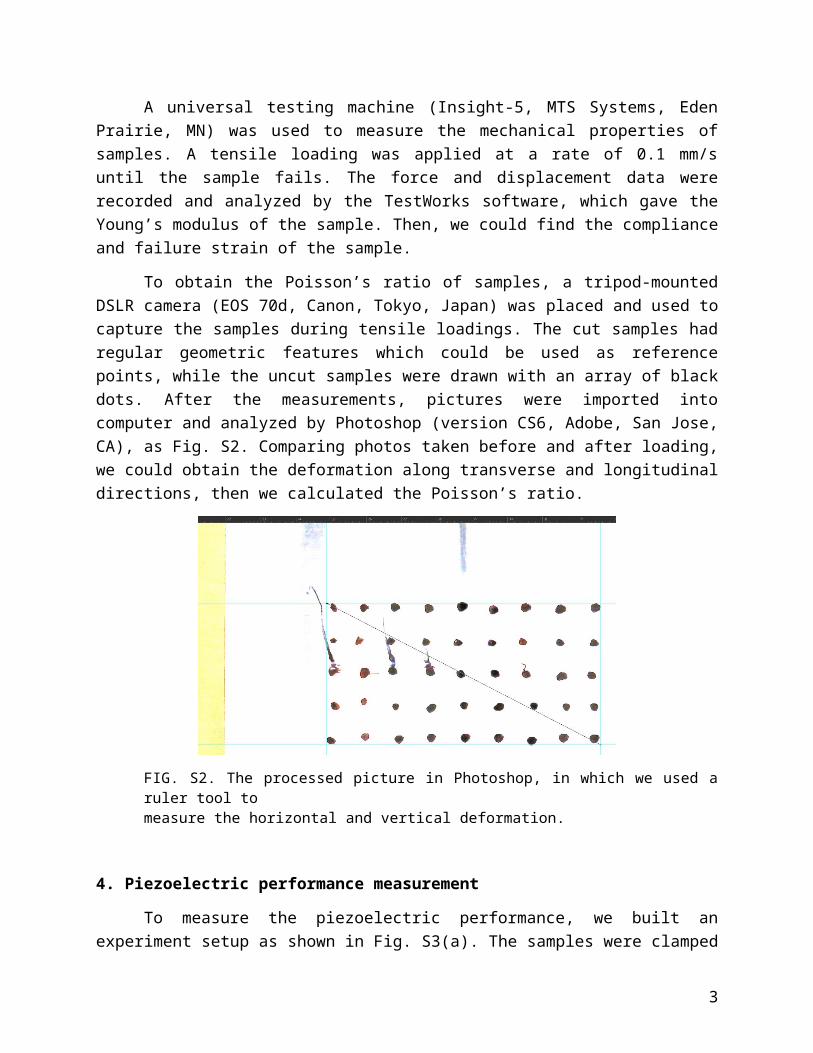
FIG. S2. The processed picture in Photoshop, in which we used a ruler tool to measure the horizontal and vertical deformation.

4. Piezoelectric performance measurement

To measure the piezoelectric performance, we built an experiment setup as shown in Fig. S3(a). The samples were clamped with one end connected to the load cell (LRM200, 10lb, Futek, Irvine, CA) fixed to the support frame and the other end connected to the shaker (APS 113, APS dynamics, San Juan Capistrano, CA), which could provide high loading force and deformation. The loading from the shaker was controlled by a synthesized function generator (DS345, Stanford Research, Sunnyvale, CA). In our tests, we set the loading to be sine waves with frequencies ranging from 10 Hz to 150 Hz. Two electrodes were attached onto both sides of the piezoelectric film. They were connected to a charge amplifier (Piezo film lab amplifier, TE Connectivity, Berwyn, PA), which converted the generated charge to voltage signal. The feedback capacitor was set to be 1 nF to match the capacitance of the sample, which was calculated from C = εA / t ~ 2 nF, where ε is the permittivity, A is the area, and t is the thickness of the film. The data were recorded by data acquisition (DAQ) system (NI-PCI 6251 and BNC-2110, National Instruments, Austin, TX) with a sampling rate at 1000 Hz. Both the mechanical and electrical data were recorded in computer and further analyzed. As shown in Figs. S3 (b)-(c), the force vs. time and charge vs. time curves were in similar shape without phase lag, indicating good time synchronization in measurements.

3

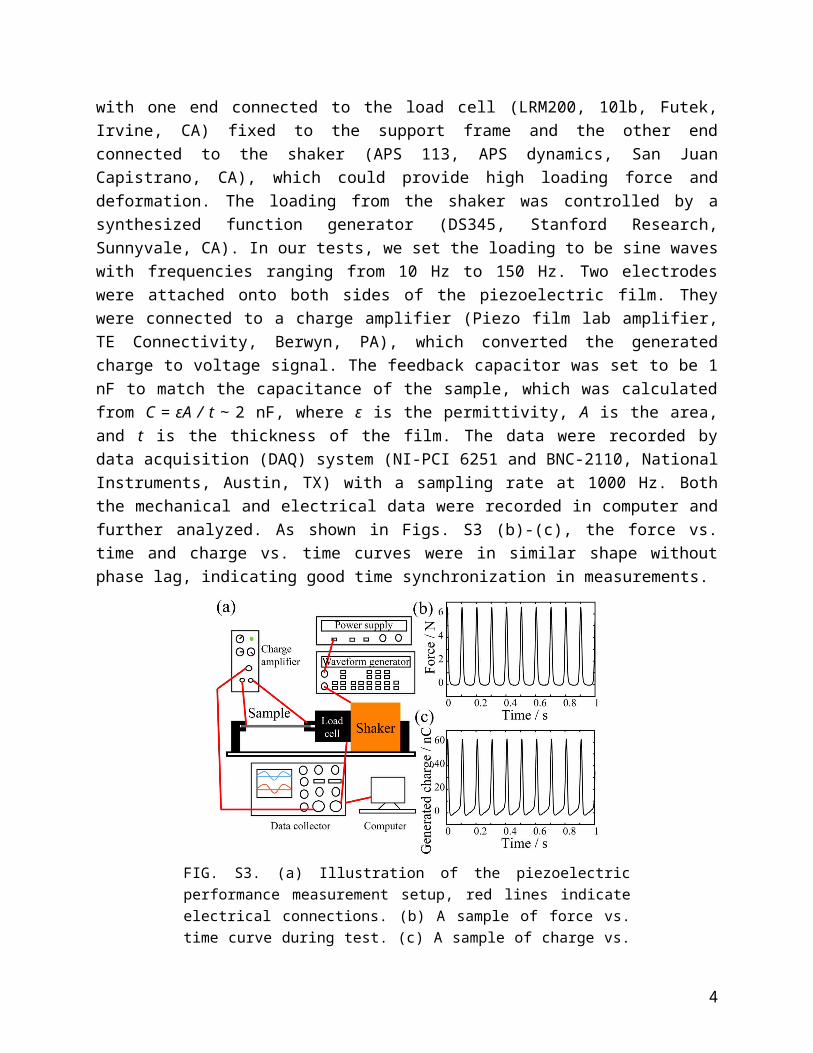
FIG. S3. (a) Illustration of the piezoelectric performance measurement setup, red lines indicate electrical connections. (b) A sample of force vs. time curve during test. (c) A sample of charge vs. time curve during test.

5. Piezoelectric test post-processing

After obtaining the force and charge data, we could calculate the effective piezoelectric constant d31

' with Eq. S1:

d31' = Qt

FL (S1)

Here Q is the generated charge, F is the applied force, and L and t are sample’s length and thickness, which are 45 mm and 0.11 mm. This equation is directly derived from Eq. 7 in the main text, according to linear piezoelectric theory. The difference is here we consider the architected thin film as a whole part regardless of its inner structure, and d31

' reflects the normalized mechanical-electrical conversion performance of a tested sample, rather than the intrinsic material property.

A MATLAB code (see below) was developed to extract the charge and force in each loading cycle, then compute the average and standard deviation of those data.

clear;clc; for I=1:15 FREQ=10*I; dir='Filelocation'; freq=num2str(FREQ); type='.lvm'; filename=strcat(dir,freq,type);

4

fid1=fopen(filename,'r'); A=textscan(fid1,'%f %f %f %f %f %f','headerlines',25); fclose(fid1); l=45; t=0.11; T=A{1}; F=A{2}; Q=A{3}; NUM=1000/FREQ; L=length(T); for i=0:(L/NUM-1) Fmax=max(F(i*NUM+1:(i+1)*NUM-1)); Fmin=min(F(i*NUM+1:(i+1)*NUM-1)); Qmax=max(Q(i*NUM+1:(i+1)*NUM-1)); Qmin=min(Q(i*NUM+1:(i+1)*NUM-1)); D(i+1)=t*(Qmax-Qmin)/(l*(Fmax-Fmin)); end d=mean(D); dd=std(D); darray(I)=d; ddarray(I)=dd;endx=10:10:150;errorbar(x,darray,ddarray);

6. Wind energy harvesting measurement

To demonstrate the application of cut samples in ambient wind energy harvesting, we performed experiments in a wind tunnel with a cross section of 0.3 m by 0.3 m. Fig. S4 shows the testing set-up for the wind energy harvesting. It is capable of producing wind within velocity range of 0 to 10 m/s. The air was driven by four computer fans (P/N PFE0381BX-000U-S99, Sunon, Kaohsiung, Taiwan) controlled by a microcontroller (Arduino UNO, Somerville, MA). The relation between input power and wind velocity was calibrated by a hand-held anemometer (866B, Holdpeak, Zhuhai, China). The sample was taped at one end and fixed on a support frame, while the other end was free. Two electrodes were attached to both surfaces of the sample and connected to charge amplifier, which transmitted the data to computer for calculating the generated power density. After recording the generated voltage during wind-tunnel tests, we converted them into power by considering the impedance value of 107 Ω.

To calculate the energy conversion efficiency, we divided the generated power by the wind power, which is the kinetic energy K divided by time t (Eq. S2):

5

Wind power= Kt

=0.5 ρAlV 2

t=0.5 ρA V 3 (S2)

whereρ is the air density, here we use the value 1.225 kg/m3 under room temperature and 1 atm; A is the area that our sample may occupy during self-flapping, which equals to the sample area in this case; Al is the volume of air passing by, so l equals to Vt, in which V is the wind velocity. At the extreme low wind velocity range, where no self-flapping is happening, the efficiency was set to 0 in order to eliminate the noises amplified by cube of velocity.

FIG. S4. Image of the wind energy harvesting system.

6