Calibration of Resistance Factors for Drilled Shafts for ... of... · Calibration of Resistance...

Murad Y. Abu-Farsakh, Ph.D., P.E.

Qiming Chen, Ph.D., P.E.

Md Nafiul Haque, MS

2013 Louisiana Transportation Conference Feb 20, 2013

Calibration of Resistance Factors for

Drilled Shafts for the 2010 FHWA

Design Method

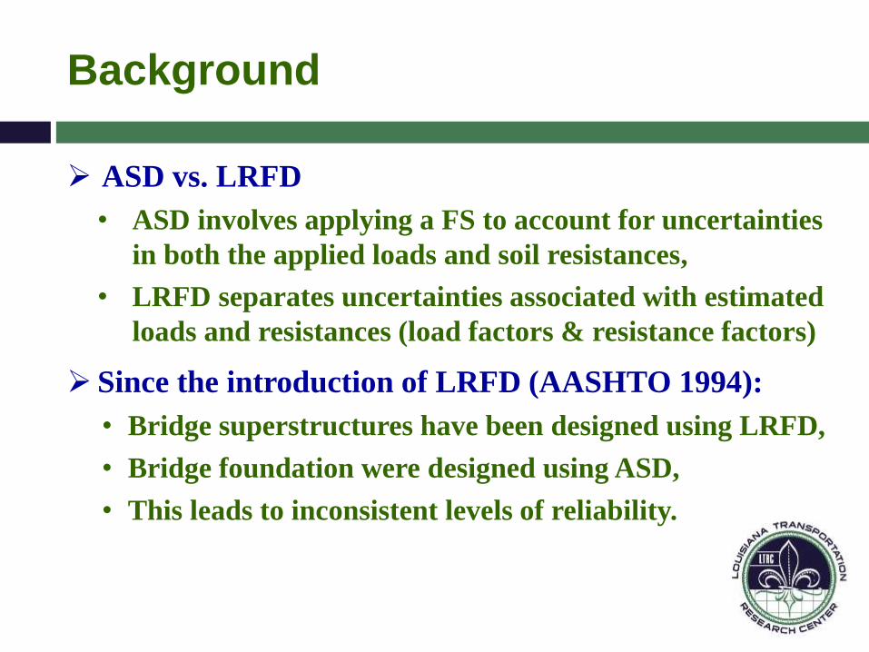
Background

ASD vs. LRFD

• ASD involves applying a FS to account for uncertainties

in both the applied loads and soil resistances,

• LRFD separates uncertainties associated with estimated

loads and resistances (load factors & resistance factors)

Since the introduction of LRFD (AASHTO 1994):

• Bridge superstructures have been designed using LRFD,

• Bridge foundation were designed using ASD,

• This leads to inconsistent levels of reliability.

Background

To maintain a consistent level of reliability, the FHWA &

ASSHTO set up a mandate date (October 1, 2007) after

which all DOT bridge projects should be designed using

LRFD method.

To comply with this, several research efforts for LRFD

calibration of 1999 FHWA drilled shafts method

• Paikowsky, 2004, UF, FHWA, and O’Neil 1996

• Allen, 2005, TRB Circular E-C079

• Yang et al. 2008, midwestern U.S., O-cell in weak rock

• Liang and Li 2009, NCHRP 24-17

• Abu-Farsakh et al. 2010 (07-2GT, Report # 470)

Background

In 2010, a new design manual (Brown et al. 2010) was

published by the FHWA in which a new design

methodology for drilled shafts was introduced,

In addition, more than 10 new drilled shaft load tests

were collected by Louisiana DOTD since the previous

study.

There is a need to calibrate the resistance factors (f)

for the 2010 FHWA design method that reflect

Louisiana soil and LA DOTD design experience.

Objectives

The main objective of this study was to calibrate

resistance factors [side (fside), tip (ftip), and total (ftotal)]

of axially loaded drilled shafts installed in Louisiana

using the 2010 FHWA drilled shafts design method

based on local load test - soil profile database, and the

LA DOTD design experience/practice.

The resistance factors for the 1999 FHWA design

method were also developed for comparison.

The target reliability value (bT) and the corresponding

resistance factor were developed for both design

methods.

ASD versus LRFD

In Allowable Stress Design (ASD)

where, Q = design load; Qall= allowable design load; Rn=

nominal (ultimate) resistance of the structure.

In Load and Resistance Factor Design (LRFD)

where, Φ = resistance factor, Rn= nominal resistance; gD = load

factor for dead load; gL= load factor for live load; QD = dead

load; and QL = live load.

FS

RQQQQ n

allLD

iiLLDDn QQQR gggf

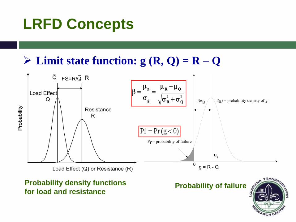
LRFD Concepts

Limit state function: g (R, Q) = R – Q

Probability density functions

for load and resistance Probability of failure

1

Q

2

R

QR

g

g

b

)0g( PrPf

LRFD Concepts

The relationship between the

probability of failure and the reliability

index (b):

The strength limit state I requires:

The limit state LRFD design equation:

f niinii RQγQ)g(R,

nii Rff nnii RQγ

)(1Pf b

Pf b

10-1 1.28

10-2 2.33

10-3 3.09

10-4 3.71

10-5 4.26

10-6 4.75

10-7 5.19

10-8 5.62

Reliability Analysis Methods

for Calibration

First order second moment method (FOSM)

• (Closed form solution)

Advanced First order second moment method (AFOSM)

First order reliability methods (FORM)

• (Iterative procedure)

Second order reliability methods (SORM)


Monte Carlo Simulation method


Calibration Methodology

Evaluate the measured (Rm) and predicted resistance

(Rp) values for drilled shafts,

Evaluate the bias factor (lR =Rm/ Rp) and COVR,

Determine distribution function (Normal, lognormal)

Formulate the limit state functions (g = R - Q)

Develop the reliability analysis procedure and

calculate reliability index (b)

Select the target reliability index (bT)

Determine the resistance factor (f) for drilled shaft

design method corresponding to bT.

Drilled Shaft Load Test Database

Approximate locations of the

investigated drilled shafts

19 cases from LA; 15 cases from MS

15 19

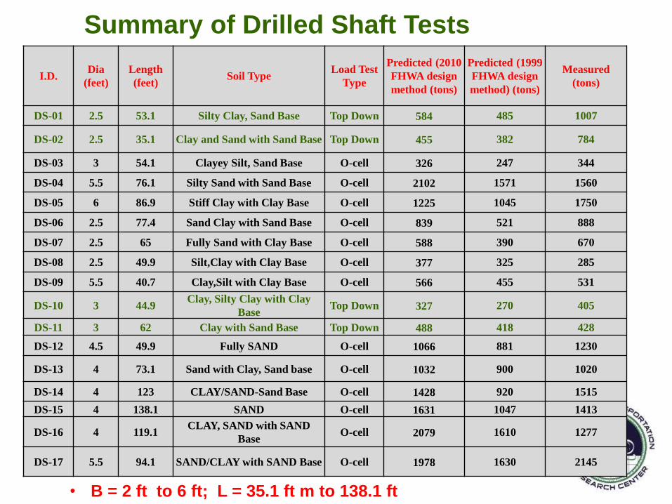
Summary of Drilled Shaft Tests

• B = 2 ft to 6 ft; L = 35.1 ft m to 138.1 ft

I.D. Dia

(feet)

Length

(feet) Soil Type

Load Test

Type

Predicted (2010

FHWA design

method (tons)

Predicted (1999

FHWA design

method) (tons)

Measured

(tons)

DS-01 2.5 53.1 Silty Clay, Sand Base Top Down 584 485 1007

DS-02 2.5 35.1 Clay and Sand with Sand Base Top Down 455 382 784

DS-03 3 54.1 Clayey Silt, Sand Base O-cell 326 247 344

DS-04 5.5 76.1 Silty Sand with Sand Base O-cell 2102 1571 1560

DS-05 6 86.9 Stiff Clay with Clay Base O-cell 1225 1045 1750

DS-06 2.5 77.4 Sand Clay with Sand Base O-cell 839 521 888

DS-07 2.5 65 Fully Sand with Clay Base O-cell 588 390 670

DS-08 2.5 49.9 Silt,Clay with Clay Base O-cell 377 325 285

DS-09 5.5 40.7 Clay,Silt with Clay Base O-cell 566 455 531

DS-10 3 44.9 Clay, Silty Clay with Clay

Base Top Down 327 270 405

DS-11 3 62 Clay with Sand Base Top Down 488 418 428

DS-12 4.5 49.9 Fully SAND O-cell 1066 881 1230

DS-13 4 73.1 Sand with Clay, Sand base O-cell 1032 900 1020

DS-14 4 123 CLAY/SAND-Sand Base O-cell 1428 920 1515

DS-15 4 138.1 SAND O-cell 1631 1047 1413

DS-16 4 119.1 CLAY, SAND with SAND

Base O-cell 2079 1610 1277

DS-17 5.5 94.1 SAND/CLAY with SAND Base O-cell 1978 1630 2145

Summary of Drilled Shaft Tests

I.D. Dia

(feet)

Length

(feet) Soil Type

Load

Test

Type

Predicted (2010

FHWA design

method (tons)

Predicted (1999

FHWA design

method) (tons)

Measured

(tons)

DS-18 4 96.1 SAND with Sand Base O-cell 1459 860 1082

DS-19 4 82 SAND/GRAVEL/Sand Base O-cell 1467 1210 1258

DS-20 4 97.1 Sand with Clay Interlayer

and Sand base O-cell 936 614 1109

DS-21 4 82 SAND with SAND Base O-cell 1159 840 875

DS-22 4 89 Clay O-cell 2558 2100 2203

DS-23 6 47.9 SAND O-cell 1585 1280 1302

DS-24 4.5 64 SAND/CLAY, Clay Base O-cell 1013 715 498

DS-25 4 64 Sand with Clay Base O-cell 600 496 445

DS-26 2 40 CLAY with Clay Base O-cell 315 262 215

DS-27 4 67.5 Fully Clay, Clay Base O-cell 425 360 549

DS-28 2.5 81.5 Fully Clay, Clay Base O-cell 455 384 570

DS-29 4 77.5 Fully Clay, Clay Base O-cell 751 639 802

DS-30 6 43 Clay, Sand with Sand Base O-cell 2431 1914 2766

DS-31 5.5 47.5 Fully Sand wth Sand Base O-cell 1874 1537 2343

DS-32 5.5 48 Sand, Clay with Sand Base O-cell 1324 1139 682

DS-33 5.5 53.85 Clay, Sand with Sand Base O-cell 1507 1347 887$

DS-34 5.5 51.12 Clay, Sand with Sand Base O-cell 1149 902 1178

• B = 2 ft to 6 ft; L = 35.1 ft m to 138.1 ft

Geotechnical Conditions

180

160

140

120

100

80

60

40

20

00 15 30 45 60

mc, LL, PL

0 50 100 150

SPT (N)

180

160

140

120

100

80

60

40

20

020 40 60 80

c (kPa)Soil Description

180

160

140

120

100

80

60

40

20

0

De

pth

(ft)

Loose tan siltLoose clayey silt

Firm to stiff silty

clay with silt

Loose sandy

silt with clay

Very dense silty

fine sand

Dense to very dense

fine sand

Very dense gray and

green silty fine sand

SPT

c

mc

LL

PL

Typical summary of geotechnical data for a tested shaft

Measured Resistance from O-Cell Test

Settlement curves by O-cell SHAFT END BEARING

SHAFT

SIDE

SHEAR

SHAFT

SIDE

SHEAR

O-cell


Equivalent top-down settlement

curve SHAFT END BEARING

SHAFT

SIDE

SHEAR

SHAFT

SIDE

SHEAR

O-cell

a) Settlement curves by O-cell b) equivalent top-down settlement curve

Determine side, tip, and total resistance at 5%B from O-cell tests

0 1 2 3 4 5 6

Load (MN)

-60

-40

-20

0

20

40

60

80

Upw

ard

To

po

fB

ott

om

O-c

ell

Mo

vem

ent

(mm

)

Dow

nw

ard

Bott

om

of

Bo

ttom

O-c

ell

Mo

vem

en

t(m

m)

0 2 4 6 8 10

Load (MN)

50

40

30

20

10

0

Se

ttle

me

nt

(mm

)

Rm-tip

Rm-side

Rm 5% B 5% B

5% B

О О

О


FHWA Design Method for Drilled Shafts

1999 FHWA Design Method for Drilled Shafts (O’Neil and Reese)

The nominal ultimate axial resistance (Rp-u) of a drilled shaft:

Rp-u = Rp-b + Rp-s = qb.Ab + ∑ fsi.Asi

Soil Condition Resistance Component Equations

Cohesive Soil

Skin Friction

End Bearing

Cohesionless

Soil

Skin Friction

End Bearing

dAf R , Sαf L

0 szs-puzzsz

ub

srrc

ubcb

3S

EI , 1) I (ln 1.33N

SNq

1.20.25

15Nfor )z 0.135/15)(1.5(Nβ

15Nfor z 0.1351.5β

dAσ'βR , tsf 2.1σ'βf

60

0.5

60

60

0.5

L

0

zs-pzSZ

b

fs

qb

Rp-u

tsf 300.6Nq SPTb

FHWA Design Method for Drilled Shafts

2010 FHWA Design Method for Drilled Shafts (Brown et al.)

The nominal ultimate axial resistance (Rp-u) of a drilled shaft:

Rp-u = Rp-b + Rp-s = qb.Ab + ∑ fsi.Asi

Soil Condition Resistance Component Equations

Cohesive Soil

Skin Friction

End Bearing

Cohesionless

Soil

Skin Friction

End Bearing

dAf R , Sαf L

0 szs-puzzsz

ub

srrc

ubcb

3S

EI , 1) I (ln 1.33N

SNq

fs

qb

Rp-u

tsf 300.6Nq SPTb

m

60

zp

L

0

zs-pzSZ

N0.47/

an)tan/)(sin-(1β

dAσ'βR , tsf) (2.1 kPa200σ'βf

a

'

p

p

p

K

fff

Predicted Resistance (1999 FHWA Method)

a) Side load transfer for cohesive soil b) End load transfer for cohesive soil

The total developed load (RT) at a specific settlement:

RT = Rp-b (developed) + Rp-s (developed)

Predicted Resistance (FHWA 2010 Method)

The total developed load (RT) at a specific settlement:

RT = Rp-sN + h Rp-bN

Normalized load transfer representing the average trend value for drilled shaft

0

50

100

150

200

0 2 4 6 8 10 12

Axia

l C

om

pre

ssio

n F

orc

eF

ailu

re T

hre

shhold

displacement dia. of shaft

Cohesionless

Cohesive

,%

,%

Failure Threshhold

Predicted Resistance (FHWA Methods)

Example of load-settlement analysis and measured value

0.0

0.5

1.0

1.5

2.0

2.5

3.0

3.5

4.0

0 200 400 600 800 1000

Dis

pla

cem

ent (i

n.)

Load (tons)

Measured Resistance

Calculated Resistance using 2010 FHWA Method

Calculated Resistance using 1999 FHWA Method

Rp RmRp

Predicted Resistance (FHWA Method)

Determine load settlement curves

Determine predicted side, tip, and total resistance

0 1 2 3 4Load (MN)

100

80

60

40

20

0

Se

ttle

me

nt(m

m)

----Predicted Resistance----Measured Resistance

5% of the shaft diameter

Shaft diameter = 1.52 m

Rp Rm

0 2 4 6Load (MN)

-200

-100

0

100

200

Se

ttle

me

nt

(mm

)

Interpreted side resistance (Rp_side)

Interpreted tip resistance (Rp_tip)

5%B

5%B

Shaft diameter = 1.52m

Measured vs. predicted resistance of drilled shafts

1999 FHWA Design Method

Results – Predicted versus Measured

1999 FHWA Design MethodRfit = 1.10Rm

0

500

1000

1500

2000

0 500 1000 1500 2000

Pre

dic

ted

Dri

lled

Sh

aft

Sid

e R

esis

tan

ce,

Rp

(to

ns)

Measured Drilled Shaft Side Resistance, Rm (tons)

Louisiana

Mississippi


0

300

600

900

1200

1500

0 300 600 900 1200 1500

Pre

dic

ted

Dri

lled

Sh

aft

Tip

Res

ista

nce

,

Rp

(to

ns)

Measured Drilled Shaft Tip Resistance, Rm (tons)

Louisiana

Mississippi

1999 FHWA design methodRfit = 0.79Rm

0

500

1000

1500

2000

2500

3000

0 500 1000 1500 2000 2500 3000

Pre

dic

ted

Dri

lled

Sh

aft

Res

ista

nce

, R

p

(ton

s)

Measured Drilled Shaft Resistance, Rm (tons)

Louisiana

Mississippi


0

300

600

900

1200

1500

0 300 600 900 1200 1500

Pre

dic

ted

Dri

lled

Sh

aft

Tip

Res

ista

nce

,

Rp

(to

ns)

Measured Drilled Shaft Tip Resistance, Rm (tons)

Louisiana

Mississippi

Measured vs. predicted resistance of drilled shafts

2010 FHWA Design Method

Results – Predicted versus Measured


0

500

1000

1500

2000

0 500 1000 1500 2000

Pre

dic

ted

Dri

lled

Sh

aft

Sid

e R

esis

tan

ce,

Rp

(to

ns)

Measured Drilled Shaft Side Resistance, Rm (tons)

Louisiana

Mississippi

2010 FHWA design methodRfit = 1.02Rm

0

500

1000

1500

2000

2500

3000

0 500 1000 1500 2000 2500 3000

Pre

dic

ted

Dri

lled

Sh

aft

Res

ista

nce

, R

p

(to

ns)

Measured Drilled Shaft Resistance, Rm (tons)

Louisiana

Mississippi

Results: Statistic Analyses

Arithmetic calculations

Best fit calculations

lR = Rm/Rp Rp/Rm

Mean σ COV Mean Rfit/Rm

0.99 0.30 0.30 1.10 1.02

Arithmetic calculations

Best fit calculations

lR = Rm/Rp Rp/Rm

Mean σ COV Mean Rfit/Rm

1.27 0.38 0.30 0.87 0.79

Statistical analysis of the 2010 FHWA drilled shaft design method

Statistical analysis of the 1999 FHWA drilled shaft design method

Histograms of bias, l, for different resistance

components – 1999 FHWA Method

0

10

20

30

40

50

60

0 1 2 3

Pro

bab

ilit

y (

%)

Rm/Rp

Log-Normal Distribution

Normal Distribution

Side Resistance (1999 FHWA design method)

0

10

20

30

0 1 2 3 4 5P

rob

ab

ilit

y (

%)

Rm/Rp


Normal Distribution

Tip Resistance (1999 FHWA design method)

0

10

20

30

40

50

0 1 2 3 4

Pro

bab

ilit

y (

%)

Rm/Rp


Normal Distribution

Total Resistance (1999 FHWA design method)

Histograms of bias, l, for different resistance

components – 2010 FHWA Method

0

10

20

30

40

50

60

0 1 2 3

Pro

bab

ilit

y (

%)

Rm/Rp


Normal Distribution

Side Resistance(2010 FHWA design method)

0

10

20

30

0 1 2 3 4 5P

rob

ab

ilit

y (

%)

Rm/Rp


Normal Distribution

Tip Resistance (2010 FHWA design method)

0

10

20

30

40

50

0 1 2 3 4

Pro

bab

ilit

y (

%)

Rm/Rp


Normal Distribution

Total Resistance (2010 FHWA design method)

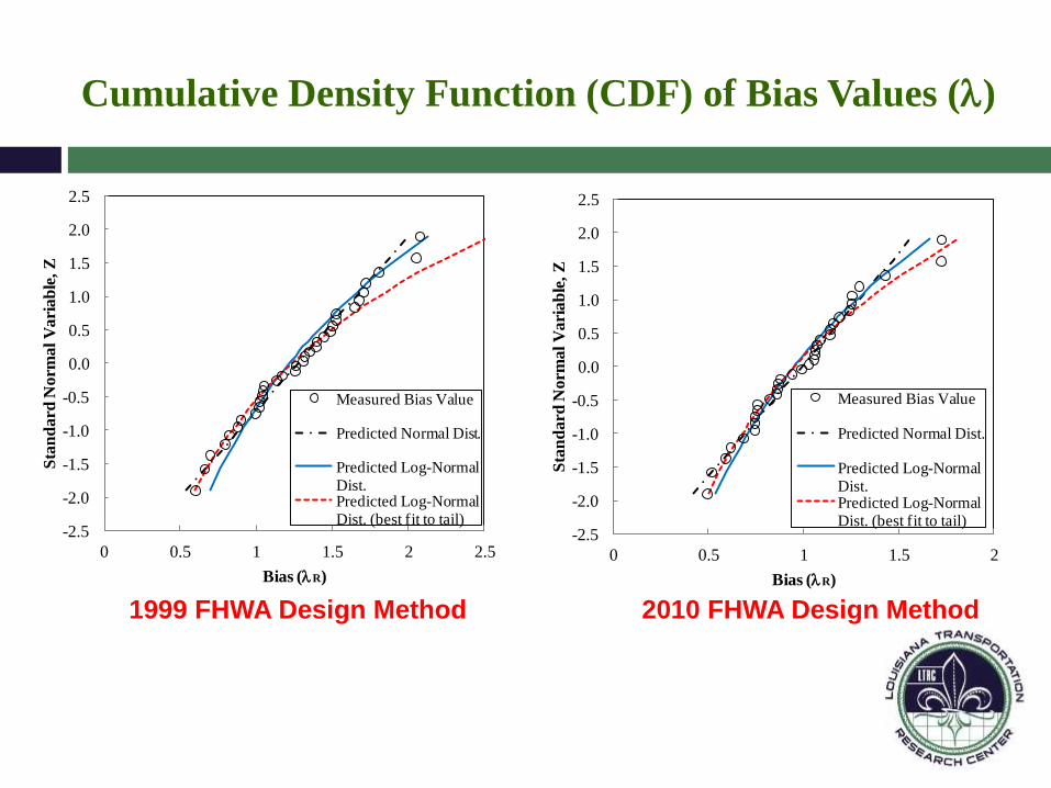
Cumulative Density Function (CDF) of Bias Values (l)

-2.5

-2.0

-1.5

-1.0

-0.5

0.0

0.5

1.0

1.5

2.0

2.5

0 0.5 1 1.5 2 2.5

Sta

nd

ard

Norm

al V

ari

ab

le, Z

Bias (lR)

Measured Bias Value

Predicted Normal Dist.

Predicted Log-Normal Dist.Predicted Log-Normal Dist. (best fit to tail)

-2.5

-2.0

-1.5

-1.0

-0.5

0.0

0.5

1.0

1.5

2.0

2.5

0 0.5 1 1.5 2S

tan

dard

Norm

al V

ari

ab

le, Z

Bias (lR)

Measured Bias Value

Predicted Normal Dist.

Predicted Log-Normal Dist.Predicted Log-Normal Dist. (best fit to tail)

2010 FHWA Design Method 1999 FHWA Design Method

Summary of Bias (l Rm/Rp) for Drilled Shafts

2010 FHWA Method

Statistics Tip Side Total

Max. 5.12 1.17 1.43

Min. 0.47 0.28 0.49

Mean (l) 2.16 0.65 0.94

COV 0.53 0.36 0.26

1999 FHWA Method

Statistics Tip Side Total

Max. 5.39 1.47 1.81

Min. 0.43 0.44 0.60

Mean (l) 2.26 0.91 1.22

COV 0.55 0.34 0.28

Contribution of Side and Tip Resistance

0

20

40

60

80

100

1 3 5 7 9 11 13 15 17 19 21 23 25 27 29 31 33

Pre

dic

ted

res

ista

nce

con

trib

uti

on

(%)

Shaft Number

Tip Resistance (average: 29%)

Side Resistance (average: 71%)

1999 FHWA Method

0

20

40

60

80

100

1 3 5 7 9 11 13 15 17 19 21 23 25 27 29 31 33

Pre

dic

ted

res

ista

nce

co

ntr

ibu

tio

n

(%)

Shaft Number


Side Resistance (average: 77%)

2010 FHWA Method

0

20

40

60

80

100

1 3 5 7 9 11 13 15 17 19 21 23 25 27 29 31 33

Mea

sure

d r

esis

tan

ce c

on

trib

uti

on

(%)

Shaft Number


Side Resistance (average: 52%) O-Cell

Measurements

LRFD Calibration Methods

Monte Carlo Simulation method (MCS method)

Target reliability index: 3.0

Dead load/Live load ratio: 3.0

Load statistics and factors (AASHTO):

Monte Carlo Simulation

Random variables:

lR, lL, and lD

Number of simulation: 50000

lglgl

f

gg

LL

DLDLDLLLLLR

LL

DLDLLL

LLQ

Q-

Q

Q

Qg

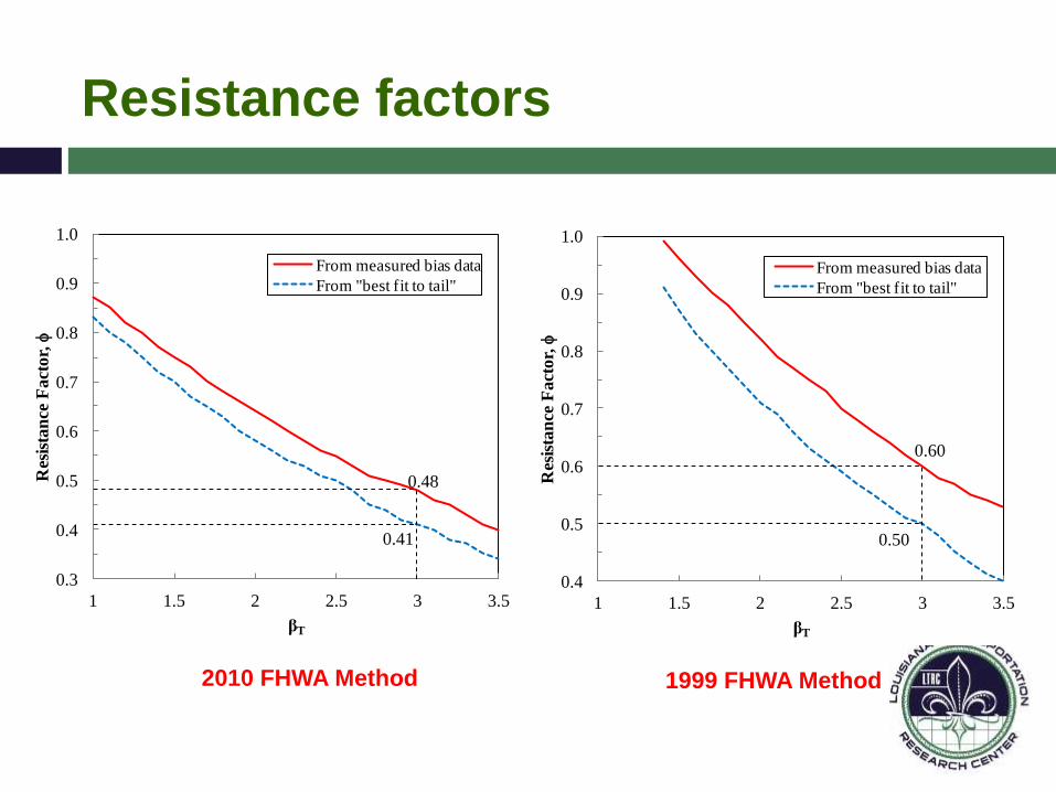
Resistance factors

2010 FHWA Method 1999 FHWA Method

0.3

0.4

0.5

0.6

0.7

0.8

0.9

1.0

1 1.5 2 2.5 3 3.5

Res

ista

nce

Fact

or,

f

βT

From measured bias data

From "best fit to tail"

0.48

0.41

0.4

0.5

0.6

0.7

0.8

0.9

1.0

1 1.5 2 2.5 3 3.5

Res

ista

nce

Fact

or,

f

βT

From measured bias data

From "best fit to tail"

0.60

0.50


Resistance Factors Tip Side Total

ftip ftip/λ fside fside/λ ftotal ftotal/λ

2010 FHWA design method 0.53 0.25 0.26 0.40 0.50 0.53

1999 design method 0.52 0.23 0.39 0.43 0.61 0.50


bT = 3.0 Resistance Factor, f Efficiency Factor, f/λ

Current study (2010

FHWA design method)

0.48 in mixed soils

0.41 in mixed soils (best fit to tail)

0.48 in mixed soils


Current study (1999

FHWA design method)

0.60 in mixed soils


0.47 in mixed soils


Liang and Li (2009)

0.45 in clay

0.50 in sand

0.35 in mixed soils

Paikowsky (2004) and

AASHTO (2007)

0.45 in cohesive soils

0.55 in cohesionless soils

Summary and Conclusions

Statistical analyses showed that:

The 2010 FHWA design method overestimates the total

drilled shaft resistance by an average of two percent,

The 1999 FHWA design method underestimates the total

drilled shaft resistance by an average of 21 percent.

The prediction of tip resistance is much more conservative

than that of side resistance. A large scatter in the

prediction of side resistance was observed.

The tip, side, and total resistance factors for drilled shafts

were calibrated using MCS reliability-based method.

The lognormal distribution of bias was assumed.

Summary and Conclusions

Based on reliability-based analyses:

• The resistance factors for 2010 FHWA method:

ftotal = 0.48, fside = 0.26, and ftip = 0.53.

• The resistance factors for 1999 FHWA method:

ftotal = 0.60, fside = 0.39, and ftip = 0.52.

Acknowledgement

Louisiana Transportation Research Center, LTRC

Louisiana Department of Transportation and

Development, LA DOTD.

THANK YOU

Questions?

Calibration of Resistance Factors for Drilled Shafts for ... of... · Calibration of Resistance...

Documents

Transcript of Calibration of Resistance Factors for Drilled Shafts for ... of... · Calibration of Resistance...