Calculus: Applications and Integrationdss.ucsd.edu/~ssaiegh/Slides3.pdf · Applications of the...

Applications of the DerivativeIntegration

Calculus: Applications and IntegrationPOLI 270 - Mathematical and Statistical Foundations

Sebastian M. Saiegh

Department of Political ScienceUniversity California, San Diego

October 7 2010

Sebastian M. Saiegh Calculus: Applications and Integration


Calculus: Applications and Integration

1 Applications of the DerivativeMean Value TheoremsMonotone Functions

2 IntegrationAntidifferentiation: The Indefinite IntegralDefinite Integrals



Mean Value TheoremsMonotone Functions

Introduction

Last week, we looked at the idea of instantaneous rate of change,and we learned how to find the derivative of a function.

Today, we are going to focus on some applications of theconcept of the derivative.

In particular, we will find out how to use derivatives to locatethe intervals in which a function is monotone and those pointsin the domain where a graph of a function presents somespecial characteristics.

These notions are critical for the study of optimization problems inpolitical science.




Local Maxima and Minima

Let f be defined on an open interval (a, b) and let x0 ∈ (a, b).

We say that f has a local maximum at x0 if f(x) ≤ f(x0).

for all values of x in some open interval I which contains x0.




Local Maxima and Minima (cont.)

Local minima are defined similarly:

f has a local minimum at x0 if f(x) ≥ f(x0)

for all values of x in some open interval I which contains x0.




Local Maxima and Minima (cont.)

In words, f has a local maximum at x0 if its graph has a “little hill”above the point x0.

Similarly, f has a local minimum at x0 if its graph has a “littlevalley” above the point x0.

If f(x0) is the maximum value of f on the whole interval (a, b),then obviously f has a local maximum at x0. But the converseneed not be true.

Absolute minima are defined similarly.




Maxima and Minima

If there is either a maximum or minimum at x = x0, we sometimescombine these two possibilities by saying f has an extremum at x0.

Notice that once we know the place (value of x) where thelargest or smallest value of f occurs, the value y = f(x) is easyto calculate.

Now, we will use a few theorems and calculus methods to locatethe appropriate x .




Locating Maxima and Minima

Theorem

Suppose that f is differentiable on (a, b) and that x0 ∈ (a, b). If fhas a local maximum or minimum at x0, then f ′(x0) = 0.




Locating Maxima and Minima (cont.)

Proof. By definition

f(x)− f(x0)

x − x0→ f ′(x0) as x → x0.

Suppose that f ′(x0) > 0.From our discussion of limits we know that if

limx→x0

f(x) = L.

then if L > 0, f(x) > 0 for some h > 0 provided thatx0 − h < x < x0 + h and x 6= x0.





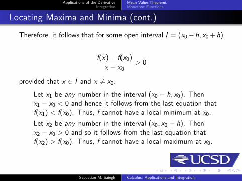
Therefore, it follows that for some open interval I = (x0−h, x0 + h)

f(x)− f(x0)

x − x0> 0

provided that x ∈ I and x 6= x0.

Let x1 be any number in the interval (x0 − h, x0). Thenx1 − x0 < 0 and hence it follows from the last equation thatf(x1) < f(x0). Thus, f cannot have a local minimum at x0.

Let x2 be any number in the interval (x0, x0 + h). Thenx2 − x0 > 0 and so it follows from the last equation thatf(x2) > f(x0). Thus, f cannot have a local maximum at x0.





A similar argument deals with the case when f ′(x0) < 0.

The only remaining possibility is f ′(x0) = 0.




Stationary Points

A point x0 at which f ′(x0) = 0 is called a stationary point of f.

Example

Let f(a) = ac + ab − a2. The value of f is zero when a = 0 andwhen a = c + b, and reaches a maximum in between.




Stationary Points (cont.)

The simplicity of the previous example is misleading, though.

In general, not every point at which the derivative of afunction is zero is a peak of its graph.

That is, not all stationary points give rise to a local maximum or alocal minimum.





For example, the derivative of the function y = x3 is zero whenx = 0, but it has neither a maximum nor a minimum at this point.





More generally, in those cases where f ′(x0) = 0 and the functionhas neither a maximum nor a minimum at that point, we say that fhas a point of inflection at x0.





The situation is further complicated by the existence of functionswith maxima or minima at points where the derivative is not evendefined. For example, consider the following function,

f(x) =

{1− x if x ≥ 01 + x if x < 0.




Rolle’s Theorem

We will now focus on a systematic procedure to locate and identifymaxima and minima of differentiable functions.

Theorem

(Rolle’s theorem) Suppose that f is continuous on [a, b] anddifferentiable on (a, b). If f(a) = f(b), then, for some x ∈ (a, b),f ′(x) = 0.




Rolle’s Theorem (cont.)

Proof. Since f is continuous on the compact interval [a, b], itfollows from the continuity property that f attains a maximum Mat some point x1 in the interval [a, b] and attains a minimum m atsome point x2 in the interval [a, b].

Suppose x1 and x2 are both endpoints of [a, b]. Becausef(a) = f(b) it then follows that m = M and hence f is aconstant on [a, b]. But then f ′(x) = 0 for all x ∈ (a, b).

Suppose that x1 is not an endpoint of [a, b]. Then x1 ∈ (a, b)and f has a local maximum at x1. Thus, f ′(x1) = 0. Similarly,if x2 is not an endpoint of [a, b].




Rolle’s Theorem (cont.)




Mean Value Theorem

Theorem

Suppose that f is continuous on [a, b] and differentiable on (a, b).

Then, for some x0 ∈ (a, b), f ′(x0) = f(b)−f(a)b−a .

In the graph, the slope of the chord PQ is f(b)−f(a)b−a . Thus, for

some x0 ∈ (a, b), the tangent of f at x0 is parallel to PQ.




Mean Value Theorem (cont.)

Theorem

Suppose that f is continuous on [a, b] and differentiable on (a, b).If f ′(x) = 0 for each x ∈ (a, b), then f is constant on [a, b].

Proof. Let y ∈ (a, b]. Then f satisfies the conditions of the meanvalue theorem on [a, y ]. Hence for some x0 ∈ (a, y),

f ′(x0) = f(y)−f(a)y−a .

But f ′(x0) = 0 and so f(y) = f(a) for any y ∈ [a, b].




Monotonicity

Let f be defined on a set S . We say that f increases on the set S ifand only if, for each x ∈ S and y ∈ S with x < y , it is true that

f(x) ≤ f(y).

If strict inequality always holds, we say that f is strictly increasingon the set S .

Similar definitions hold for decreasing and strictly decreasing.

A function that is either increasing or decreasing is calledmonotone.

A function which is both increasing and decreasing must be aconstant.




Strictly Increasing Functions

Example

The function f : R→ R defined by f(x) = x3 is strictly increasingon R.




Strictly Decreasing Functions

Example

The function f : (0,∞)→ R defined by f(x) = 1x is strictly

decreasing on (0,∞).




Increasing and Decreasing Functions

We can observe that a function is increasing if its graph is rising asx increases and decreasing if its graph is falling as x increases.

This function, for example, is increasing for a < x < b and forx > c . It is decreasing for x < a and for b < x < c .




Local Maxima and Minima

If we know the intervals on which a function is increasing anddecreasing, we can easily identify its local maxima and minima.

A local maximum occurs when the function stops increasingand starts decreasing.

In the previous graph, this happens when x = b.

A local minimum occurs when the function stops decreasingand starts increasing.

In this case, this happens when x = a and x = c .




Differentiable monotone functions

Notice that we can find out where a differentiable function isincreasing or decreasing by checking the sign of its derivative.

Theorem

Suppose that f is continuous on [a, b] and differentiable on (a, b).

(i) If f ′(x) ≥ 0 for each x ∈ (a, b), then f is increasing on [a, b].If f ′(x) > 0 for each x ∈ (a, b), then f is strictly increasing on[a, b].

(ii) If f ′(x) ≤ 0 for each x ∈ (a, b), then f is decreasing on [a, b].If f ′(x) < 0 for each x ∈ (a, b), then f is strictly decreasing on[a, b].




Differentiable monotone functions (cont.)

Proof. Let c and d be any numbers in [a, b] which satisfy c < d .Then f satisfies the conditions of the mean value theorem on [c , d ]and hence, for some x0 ∈ (c , d),

f ′(x0) =f(d)− f(c)

d − c.

If f ′(x) ≥ 0 for each x ∈ (a, b), then f ′(x0) ≥ 0 and hencef(d) ≥ f(c). Thus f increases on [a, b].

If f ′(x) > 0 for each x ∈ (a, b), then f ′(x0) > 0 and hencef(d) > f(c). Thus f is strictly increasing on [a, b].

Similarly, for the other cases.





Example

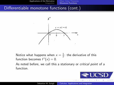
Consider the function f : R→ R defined by f(x) = x(1− x).

The derivative of this function is given by f ′(x) = 1− 2x .

Hence, f ′(x) ≥ 0 when x ≤ 12 and f ′(x) ≤ 0 when x ≥ 1

2 .

It follows that f increases on (−∞, 12 ] and decreases on [ 1

2 ,∞).





Notice what happens when x = 12 : the derivative of this

function becomes f ′(x) = 0.

As noted before, we call this a stationary or critical point of afunction.




Critical Points

Critical Point. A point x in the feasible set of a functionf(x) is a critical point for f if df

dx= 0 there, or the derivative

is undefined.

Every local extremum is a critical point.

However, as we saw earlier, not every critical point isnecessarily a local extremum.




Critical Points (cont.)

If the derivative is positive to the left of a critical point andnegative to the right of it, the function changes from increasing todecreasing and the critical point is a local maximum.

If the derivative is negative to the left of a critical point andpositive to the right of it, the function changes fromdecreasing to increasing and the critical point is a localminimum.

If the sign of the derivative is the same on both sides of the criticalpoint, the critical point is neither a local maximum nor a localminimum.




Higher-Order Derivatives

If a function y = f(x) is differentiable, its derivative is anotherfunction f ′(x).

If f ′(x) is itself differentiable, we can apply the differentiationprocess to it.

The resulting function, called the second derivative, is denoted byany one of the following interchangeable symbols:

d2ydx2 = d

dx (dydx ), d2f

dx2 , y ′′, f ′′, f (2)




Higher-Order Derivatives (cont.)

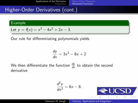
Example

Let y = f(x) = x3 − 4x2 + 2x − 3.

Our rule for differentiating polynomials yields

dy

dx= 3x2 − 8x + 2

We then differentiate the function dydx to obtain the second

derivative

d2y

dx2= 6x − 8.




Higher-Order Derivatives (cont.)

There is no reason why this process cannot be continued, providedthat we obtain differentiable functions at each step.

Differentiating the second derivative, we obtain a newfunction called the third derivative; differentiating the thirdderivative yields the fourth derivative, and so on.

We are particularly interested in the second derivative, though,because there is a very useful geometric interpretation of it.




Concavity

We can see the usefulness of the second derivative by looking atthe notion of concavity.

A curve is said to be concave upward if the slope of itstangent increases as it moves along the curve from left toright.

A curve is said to be concave downward if the slope of itstangent decreases as it moves along the curve from left toright.




Concavity (cont.)

This picture illustrates the idea of concavity. The curve is concaveupward to the left of x = a and concave downward to the right.

A useful “trick” : a graph can be described as “holdingwater” where it is concave upward, and as “spilling water”where it is concave downward.




Concavity (cont.)

There is a simple characterization of concavity in terms of the signof the second derivative.

It is based on the fact (established earlier in this class) that aquantity increases when its derivative is positive and decreaseswhen its derivative is negative.

The second derivative comes into the picture when this fact isapplied to the first derivative (or slope of the tangent).




Concavity (cont.)

Here is the argument: suppose the second derivative f ′′ is positiveon an interval.

This implies that the first derivative f ′ must be increasing onthe interval. But f ′ is the slope of the tangent.

Hence, the slope of the tangent is increasing, and so the graph of fis concave upward on the interval.

On the other hand, if f ′′ is negative on an interval, then f ′ isdecreasing. This implies that the slope of the tangent isdecreasing, and so the graph of f is concave downward on theinterval.




Test for Concavity

Test for Concavity.

If f ′′(x) > 0 on the interval a < x < b, then f is concaveupward on this interval.

If f ′′(x) < 0 on the interval a < x < b, then f is concavedownward on this interval.




Test for Concavity (cont.)

We have to be careful, though. You should not confuse theconcavity of a curve with its increase or decrease.

A curve that is concave upward on an interval may be eitherincreasing or decreasing on that interval.

Similarly, a curve that is concave downward may be increasing ordecreasing.





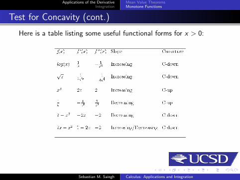
Here is a table listing some useful functional forms for x > 0:




Using the second derivative to find extrema

We can also use the second derivative to identify whether there isa point on the graph of a function at which the concavity of thefunction changes.

We usually call this point an inflection point.

If the second derivative of a function is defined at aninflection point, its value there must be zero.

Inflection points can also occur at points in the domain of thefunction where the second derivative is undefined.




Using the second derivative to find extrema (cont.)

Points on the graph of a function f(x) where f ′(x) = 0 or f ′(x)does not exist are sometimes called first-order critical points.

A number c in the domain of f where f ′′(c) = 0 or f ′′(x)does not exist is called a second-order critical value, and thecorresponding point (c , f(c)) on the graph of f is called asecond-order critical point.

Second-order critical points are to inflection points as first-ordercritical points are to local extrema.

In particular, every inflection point is a second-order criticalpoint.




The Second Derivative Test

The second derivative can also be used to classify the first-ordercritical points of a function as local maxima or local minima.

The procedure is usually known as the second derivative test.

The Second Derivative Test.Suppose f ′(a) = 0.If f ′′(a) > 0, then f has a local minimum at x = a.If f ′′(a) < 0, then f has a local maximum at x = a.However, if f ′′(a) = 0, the test is inconclusive and f may havea local maximum, a local minimum, or no local extremum atall at x = a.




The Second Derivative Test (cont.)

Example

Let f(x) = 2x3 + 3x2 − 12x − 7. We will use the second derivativetest to find the local extrema.

First, we calculate the first derivative of this function,

f ′(x) = 6x2 + 6x − 12

We can now re-write this expression as 6(x + 2)(x − 1) to seemore easily how f ′(x) = 0 when x = −2 and when x = 1.

And that their corresponding points (−2, 13) and (1,−14) arethe first-order critical points of f.




The Second Derivative Test (cont.)

Next, to test these points we compute the second derivative

f ′′(x) = 12x + 6

and we evaluate it at x = −2 and x = 1.

Since f ′′(−2) = −18 < 0, it follows that the critical point(−2, 13) is a local maximum.

And since f ′′(1) = 18 > 0, it follows that the critical point(1,−14) is a local minimum.




Absolute Maxima and Minima

We already know how to find local extrema, right?

But suppose we want to find now the absolute maximum (orminimum) of some function f.

We already know that places where the derivative is equal to zeroare important, so we can use the notion of a critical point to locatethe absolute extremum.




Absolute Maxima and Minima (cont.)

Locating Absolute Extrema on a Bounded Interval. Supposef is differentiable on a closed, bounded interval a ≤ x ≤ b.

Step 1 Locate all critical points x1, ..., xk within the interval.

Step 2 Calculate the values y = f(x) at these critical points andat the endpoints x = a and x = b.

Step 3 Compare the values f(a), f(x1), ..., f(xk), f(b). The largestof these is the absolute maximum for f on the interval a ≤ x ≤ b;the smallest is the absolute minimum.





Notice that when the interval on which we wish to maximize orminimize a continuous function is not of the form a ≤ x ≤ b, thisprocedure no longer applies.

This is because there is no longer any guarantee that thefunction actually has an absolute maximum or minimum onthe interval in question.

On the other hand, if an absolute extremum does exist and thefunction is continuous on the interval, the absolute extremum willstill occur at a local extremum or endpoint contained in theinterval.





Therefore, to find the absolute extrema of a continuous functionon an interval that is not of the form a ≤ x ≤ b, we still evaluatethe function at all the critical points and endpoints that arecontained in the interval.

It turns out that in many cases, the interval at hand willcontain only one first-order critical value of the function.

When this happens, we can use the second derivative test toidentify its absolute extremum, even though this test is reallya test for only local extrema.

The reason is that, in this special case, every local maximum orminimum is necessarily also an absolute maximum or minimum.




Second Derivative Test for Absolute Extrema

The Second Derivative Test for Absolute Extrema. Supposethat f is continuous on an interval on which x = a is the onlyfirst-order critical value and that f ′(a) = 0.

If f ′′(a) > 0, then f(a) is the absolute minimum of f on theinterval.If f ′′(a) < 0, then f(a) is the absolute maximum of f on theinterval.

The second derivative test for absolute extrema can be applied toany interval, whether closed or not.

The only requirement is that the function be continuous andhave only one critical value on the interval.



Antidifferentiation: The Indefinite IntegralDefinite Integrals







Introduction

Differentiation is one of the two central concepts in calculus.

The other one is integration.

The first operation, calculating the derivative of a function, is usedto find the exact slope of the tangent to a function’s curve at anyspecified point along the curve.

The second operation, integration, can be used to find thearea under the graph of a continuous function.




Introduction (cont.)

Both problems, finding the tangent (to) and the area (under) acurve, can be solved following different and independent paths, butat the end of the day, they are inter-related as the calculation ofareas can be reduced to the calculation of the antiderivative of afunction.

In practical terms, integration comes in handy when thederivative of a function is known and the goal is to find thefunction itself.

For example, say we know the rate of inflation, we may wish to usethis information to estimate future prices.




Antiderivative

In a sense, integration is the inverse of differentiation, so a goodstarting point is to say a few words about reversing the process ofdifferentiation.

An indefinite integral or antiderivative of a function f(x) isany function F (x) whose derivative is the original function

dF

dx= f(x).

For example, what is an indefinite integral for f(x) = x2? We wantto find a function F (x) whose derivative is f(x) = x2.




Antiderivative (cont.)

This is a new and unfamiliar problem.

However, we do know a lot about derivatives, so it is not hardto make an informed guess.

Recall the power rule: the derivative of any power x r is aconstant times a power of one lower degree.

If we want to find a function F (x) such that dFdx = x2, this

suggests we consider something like x3. Now

d

dx(x3) = 3x2

so F (x) = x3 is not quite the correct choice.





However, if we choose F (x) = 13 x3 then

dF

dx=

d

dx

(1

3x3)

=1

3

d

dx(x3) =

1

3(3x2) = x2.

Thus, F (x) = 13 x3 is an indefinite integral of f(x) = x2.





Example

Let F (x) = 13 x3 + 5x + 2. Can F (x) be the antiderivative of

f(x) = x2 + 5?

Well, F (x) is an antiderivative of f(x) if and only if F ′(x) = f(x).

As we differentiate F we find that

dF

dx= x2 + 5 = f(x).





A function f(x) may have more than one indefinite integral.

For example, one antiderivative of the function f(x) = 3x2 isF (x) = x3, since

d

dx(x3) = 3x2 = f(x).

But so is G (x) = x3 + 12, since the derivative of the constant12 is zero and

d

dx(x3 + 12) = 3x2 = f(x).





In general, if F is one antiderivative of f, any function obtained byadding a constant to F is also an antiderivative of f.

This leads us to ask: How can we find all indefinite integralsof a function f(x)?

Given one indefinite integral F (x), there are others of the form

F (x) + constant.

In fact, these are all there are.




Uniqueness of the Indefinite Integral

In other words, if f(x) has an indefinite integral at all, thisindefinite integral is “unique up to an added constant.”

For example, f(x) = x2 has F (x) = 13 x3 as an indefinite

integral; all possible indefinite integrals are of the form

1

3x3 + c (c any constant).

Uniqueness of the Indefinite Integral. Suppose that f(x) hasan indefinite integral F (x) on an interval. Then all other indef-inite integrals of f(x) have the form F (x) + c , where c is anarbitrary constant.




Uniqueness of the Indefinite Integral (cont.)

Proof. Suppose G (x) is any other indefinite integral for f(x). Then

dF

dx= f(x) and

dG

dx= f(x).

Their difference H(x) = G (x)− F (x) has derivative zero because

dH

dx=

d

dx(G (x)− F (x)) =

dG

dx− dF

dx= f(x)− f(x) = 0.

That is, the rate of change of H(x) is identically zero for all x .Intuitively, we can see that this forces H(x) to be a constantfunction, H(x) = c for all x (c some constant).

Because G (x)− F (x) = c , we obtain G (x) = F (x) + c .




Integral Notation

Indefinite integrals of f(x) are indicated by the special symbol∫f(x)dx

The symbol∫

is called an integral sign and indicates that you areto find the most general form of the antiderivative of the functionfollowing it.

The integral sign is merely an elongated “s”, and stands for“the sum of”. In the expression∫

f(x)dx ,

the function f(x) that is to be integrated is called theintegrand.




Integral Notation (cont.)

The symbol dx that appears after the integrand may seemmysterious. Its role is to indicate that x is the variable with respectto which the integration is to be performed.

The symbol d merely means “a little bit of.” Thus, dx meansa little bit of x , and

∫dx means the sum of all the little bits

of x .

Hence, it is customary to write∫f(x)dx = F (x) + c

to express the fact that every antiderivative of f(x) is of theform F (x) + c .




Integral Notation (cont.)

Example

Let f(x) = 3x2.

We can express the fact that every antiderivative of f is of the formx3 + c by writing

∫3x2dx = x3 + c .

In the above expression∫f(x)dx = F (x) + c

the function f is the integrand, and the (unspecified) constantc that is added to F (x) to give the most general form of theantiderivative is known as the constant of integration.




The Indefinite Integral

Here is a restatement of the definition of the indefinite integral (orantiderivative) in integral notation.

The Indefinite Integral.∫f(x)dx = F (x) + c

if and only if

F ′(x) = f(x)

for every x in the domain of f.




Integration Rules

As stated before, integration is the reverse of differentiation.

Therefore, many rules for integration can be obtained bystating the corresponding rules for differentiation in reverse.

Example

Let f(x) = x7. An indefinite integral of f is given by F (x) = 18 x8:

dF

dx=

d

dx

(1

8x8)

= x7.




Integration Rules (cont.)

More generally, by reversing the differentiation formula

d

dx

( 1

r + 1x r+1

)=

r + 1

r + 1x r = x r

we see that the function f(x) = x r has an indefinite integral of theform

F (x) =x r+1

r + 1

except when r = −1, in which case 1r+1 is undefined.




Power Rule for Integrals

The Power Rule for Integrals. For r 6= −1,∫x r dx =

x r+1

r + 1+ c

That is, to integrate x r (for r 6= −1), increase the power of x by1 and divide by the new power.




Power Rule for Integrals (cont.)

Example

Let f(x) = x35

To find the indefinite integral we should simply increase the powerof x by 1 and then divide by the new power to get∫

x35 dx =

5

8x

85 + c

Example

Let f(x) = 1x3

The function f has an indefinite integral

F (x) =x−3+1

−3 + 1=

x−2

−2=−1

2x2.





Example

Let f(x) =√

x

The function f has an indefinite integral

F (x) =x

12

+1

12 + 1

=x

32

32

=2

3x

32 .

This is the first of several integration rules we shall derive.





To avoid errors, some special indefinite integrals are worth noting.

The constant function f(x) = x0 has indefinite integral

F (x) =x1

1= x .

The function f(x) = x−1 has indefinite integral∫1

xdx = ln |x |+ c

When x is negative, it turns out that the function ln |x | is anantiderivative of 1

x , because if x is negative, then |x | = −x and

d

dx(ln |x |) =

d

dx[ln(−x)] =

( 1

−x

)(−1) =

1

x.





The function ex has indefinite integral∫exdx = ex + c

Integration of the exponential function ex is trivial since ex is itsown derivative.




Constant Multiple Rule for Integrals

The Constant Multiple Rule for Integrals.

For any constant c ,∫cf(x)dx = c

∫f(x)dx

That is, the integral of a constant times a function is equal tothe constant times the integral of the function.




Constant Multiple Rule for Integrals (cont.)

Again, some special indefinite integrals are worth noting.

The constant function whose value is k , f(x) = k hasF (x) = kx for an indefinite integral. This gives the integrationformula ∫

kdx = kx + c (k any constant)

Taking k = 1 or k = 0 we get to commonly encounteredspecial cases: ∫

1dx = x + c

∫0dx = c




Sum Rule for Integrals

The Sum Rule for Integrals.∫[f(x) + g(x)]dx =

∫f(x)dx +

∫g(x)dx

That is, the integral of a sum is the sum of the individualintegrals.




Sum Rule for Integrals (cont.)

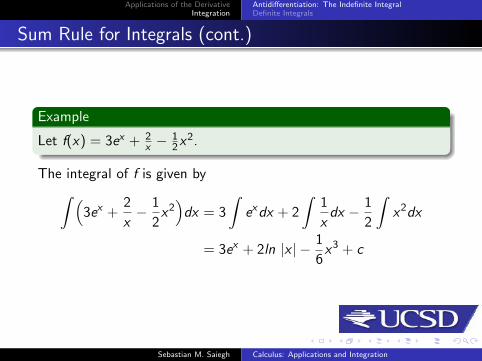
Example

Let f(x) = 3ex + 2x −

12 x2.

The integral of f is given by∫ (3ex +

2

x− 1

2x2)

dx = 3

∫exdx + 2

∫1

xdx − 1

2

∫x2dx

= 3ex + 2ln |x | − 1

6x3 + c




Integration of Products and Quotients

You may have noticed that we did not look at any general rules forthe integration of products and quotients.

This is because there are no general rules.

Occasionally, we may be able to rewrite a product or a quotient ina form in which you can integrate it using the techniques we havelearned today.




Integration of Products and Quotients (cont.)

Example

Let f(x) = 3x5+2x−5x3 .

We can rewrite f as

3x5 + 2x − 5

x3= 3x2 +

2

x2− 5

x3= 3x2 + 2x−2 − 5x−3

and then integrate term by term:∫3x5 + 2x − 5

x3dx =

∫(3x2 + 2x−2 − 5x−3)dx

= x3 − 2x−1 +5

2x−2 + c

= x3 − 2

x+

5

2x2+ c




Practical Application

Lets look at a concrete problem in which the rate of change of aquantity is known and the goal is to find an expression for thequantity itself.

Since the rate of change is the derivative of the quantity, wecan find the expression for the quantity itself byantidifferentiation.

Example

A manufacturer has found that marginal cost is 3q2 − 60q + 400dollars per unit when q units have been produced. The total costof producing the first 2 units is $900. What is the total cost ofproducing the first 5 units?




Practical Application

First, note that the marginal cost is the derivative of the total costfunction C (q).

Thus, C ′(q) = 3q2 − 60q + 400 and so C (q) must be theantiderivative

C (q) =

∫C ′(q)dq =

∫(3q2 − 60q + 400)dq = q3 − 30q2 + 400q + k

for some constant k .The value of k is determined by the fact that C (2) = 900:

900 = (2)3 − 30(2)2 + 400(2) + k or k = 212




Practical Application (cont.)

Therefore,

C (q) = q3 − 30q2 + 400q + 212

and the cost of producing the first 5 units is

C (5) = (5)3 − 30(5)2 + 400(5) + 212

which amounts to $1,587.




Definite Integral: Definition

We have already learned the techniques of antidifferentiation.

Now, we are going to define the definite integral of a functionin terms of its indefinite integral and use it to calculate areas.

We start by defining the definite integral of a function f(x)over the interval a ≤ x ≤ b. It is indicated by the symbol∫ b

af(x)dx

The number b is called the “upper limit,” and a is the “lowerlimit” of the definite integral.

In contrast with the indefinite integral, which is a function,the definite integral is a number.




Calculating the Definite Integral

Rule for Calculating the Definite Integral. Let∫ ba f(x)dx

Step 1 Find an indefinite integral F (x) of f(x) on the intervala ≤ x ≤ b.

Step 2 Compute the value of the indefinite integral F (x) atthe upper limit x = b; this is F (b).

Step 3 Compute the value of F (x) at the lower limit x = a;this is F (a).

Step 4 Subtract the number in Step 3 from the number inStep 2; this is the definite integral∫ b

af(x)dx = F (b)− F (a)




Calculating the Definite Integral (cont.)

In carrying out this procedure it does not matter which indefiniteintegral F (x) we use; the number obtained in Step 4 will always bethe same.

To see why, observe that if G (x) is some other indefiniteintegral of f(x), then G (x) = F (x) + c for some constant c .

Therefore

G (b)− G (a) = (F (b) + c)− (F (a) + c)

= F (b) + c − F (a)− c

= F (b)− F (a)

and the added constant c cancels out of the final result.





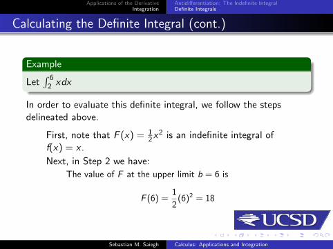
Example

Let∫ 6

2 xdx

In order to evaluate this definite integral, we follow the stepsdelineated above.

First, note that F (x) = 12 x2 is an indefinite integral of

f(x) = x .

Next, in Step 2 we have:

The value of F at the upper limit b = 6 is

F (6) =1

2(6)2 = 18





In Step 3 we have:

The value of F at the lower limit a = 2 is

F (2) =1

2(2)2 = 2

Finally, in step 4 we obtain the definite integral by taking thedifference of these values,∫ 6

2xdx = F (6)− F (2) = 18− 2 = 16





With practice, the steps in this procedure can be combined byintroducing a useful symbol used universally to indicate thedifference of endpoint values of a function F (x).

If we define F (x)∣∣∣ba

= F (b)− F (a), the procedure for

calculating the definite integral takes on a simple form.

∫ b

af(x)dx = F (x)

∣∣∣ba

where F (x) is any indefinite integral of f.





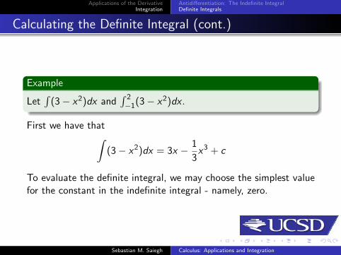
Example

Let∫

(3− x2)dx and∫ 2−1(3− x2)dx .

First we have that∫(3− x2)dx = 3x − 1

3x3 + c

To evaluate the definite integral, we may choose the simplest valuefor the constant in the indefinite integral - namely, zero.





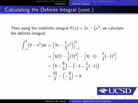
Then using the indefinite integral F (x) = 3x − 13 x3, we calculate

the definite integral:∫ 2

−1(3− x2)dx =

(3x − 1

3x3)∣∣∣2−1

=[3(2)− 1

3(2)3

]−[3(−1)− 1

3(−1)3

]=(

6− 8

3

)−(−3− 1

3(−1)

)=

10

3−(−8

3

)= 6




Areas

Finally, we now turn to the problem of area. We shall considergeneral regions in the plane such as the one shown in the followingfigure.

Such a region R is obtained by taking the part of the planebounded by a continuous curve y = f(x), the x axis, and the twovertical lines x = a and x = b.




Fundamental Theorem of Calculus

We will assume that a < b, as in the figure, and restrict theattention to the case where f(x) ≥ 0; so the curve y = f(x) staysabove the horizontal axis.

Then the area, Area(R), can be evaluated by applying a trulyremarkable result connecting areas and integrals.

Fundamental Theorem of Calculus. For any plane region R ofthe form shown in the previous figure, bounded by the graph of acontinuous function y = f(x), the area of R is equal to the definiteintegral of f(x) for a ≤ x ≤ b:

Area(R) =

∫ b

af(x)dx




Fundamental Theorem of Calculus (cont.)

Example

Let f(x) = 3, for 1 ≤ x ≤ 5. The region R bounded by the graphof f is a rectangle.





We can now use the Fundamental Theorem of Calculus to get thearea for R. Its upper boundary is given by the constant functionf(x) = 3, and the vertical lines are given by a = 1 and b = 5.

Using the Fundamental Theorem of Calculus and theindefinite integral F (x) = 3x we obtain

Area(R) =

∫ b

af(x)dx =

∫ 5

13dx

= 3x∣∣∣51

= 15− 3

= 12

Note that this calculation agrees with the usual formula:Area = height × width, because the height is 3, and the width is5-1=4.





Lets examine now a region whose area cannot be calculated by theusual methods of plane geometry (finding its area would bedifficult without the Fundamental Theory of Calculus).

Example

Let f(x) = x2, for −1 ≤ x ≤ 2. The area R of the region lyingabove the interval in the x axis and below the graph of f looks likethis.





The upper boundary of R is given by y = x2, and the verticalboundary lines are given by a = −1 and b = 2.

We have already found indefinite integrals for f(x) = x2 at thebeginning of today’s class.

We may use the particular indefinite integral F (x) = 13 x3.





Applying the Fundamental Theorem we obtain,

Area(R) =

∫ 2

−1x2dx

=1

3x3∣∣∣2−1

=(1

3(2)3

)−(1

3(−1)3

)=(8

3

)−(−1

3

)=

9

3= 3


Calculus: Applications and Integrationdss.ucsd.edu/~ssaiegh/Slides3.pdf · Applications of the...

Documents

Transcript of Calculus: Applications and Integrationdss.ucsd.edu/~ssaiegh/Slides3.pdf · Applications of the...