Calculation of FSA method
28
A method for measuring frontal surface area Developed by Andrew D. Moss for use by British Cycling Project documentation: part of the 2002/3 World Class Sport Science Development Programme – a BASES/UKSI project collaboration.
-
Upload
andrew-moss -
Category
Documents
-
view
112 -
download
0
Transcript of Calculation of FSA method
A method for measuring frontal surface area
Developed by
Andrew D. Moss for use by British Cycling
Project documentation: part of the 2002/3 World Class Sport Science
Development Programme – a BASES/UKSI project collaboration.

List of contents
Title page...................................................................................................................................1
List of contents..........................................................................................................................2
1. Introduction...........................................................................................................................3
1.1. Pilot work experimental setup..........................................................................................4
1.1.2. Camera position............................................................................................................4
1.1.3. Calibration board position...........................................................................................4
1.2. Data collection experimental setup..................................................................................6
1.2.1. Camera position............................................................................................................6
1.2.2. Subject position.............................................................................................................6
1.2.3. Camera Setup................................................................................................................7
1.3. Pilot data collection............................................................................................................9
1.3.1. Measurement validity...............................................................................................91.3.2. Perspective error.......................................................................................................91.3.3. Measurement reliability..........................................................................................10
1.4. Results of pilot data collection.......................................................................................101.4.1. Measurement validity.............................................................................................101.4.2. Perspective error.....................................................................................................111.4.3. Measurement reliability..........................................................................................12
1.5. Sport specific pilot data collection................................................................................121.5.1. Assessment of three riding positions......................................................................121.5.2. Measurement reliability..........................................................................................131.5.3. Isolated assessment of subject and cycle................................................................13
1.6. Results of sport specific pilot data collection................................................................141.6.1. Assessment of three riding positions......................................................................141.6.2. Measurement reliability..........................................................................................141.6.3. Isolated assessment of subject and cycle................................................................14
2. Data collection with Great Britain Endurance Squad....................................................15
3. Guidelines for calculation of FSA from digital images........................................................15
2
1. Introduction
Collaboration between BASES (British Association of Exercise and Sport Sciences) and the
UKSI (United Kingdom Sports Institute) resulted in nine positions for developing sport
scientists to work, through placement, with specific sports. Each position required the
associated placement individual to complete a specified number of contact hours and a project
mutually agreed by the sport supervisor, BASES supervisor and the placement individual in
the period May 2002 to May 2003.
This method document serves as proof of the completion of a project identified by Andrea
Wooles (sport supervisor: British Cycling) and agreed by Dr Andrew Jones (Bases
Supervisor) and Andrew D. Moss (placement individual). The agreed project was to develop a
method of measuring frontal surface area (FSA) to be used by British Cycling with the
ultimate aim of improving the performance of British cyclists.
The results of the pilot work are presented first. Data collected from the 2003 Great Britain
Endurance Squad using the developed method for measuring FSA is then presented. Finally,
detailed guidelines for equipment setup, image manipulation and measurement are provided.
3

1.1. Pilot work experimental setup
The experimental setup is shown in figure 1.
1.1.2. Camera position
Height – the centre of the lens should be positioned at the same height as the centre of
the calibration board.
Distance from calibration board – minimum horizontal distance of 8 m was observed
between the camera and the calibration board. The scaling object was aligned
vertically with the frontal plane of the calibration board. The camera zoom facility was
used to select an appropriate image size. This process was performed in order to
minimise perspective error.
1.1.3. Calibration board position
The calibration board was positioned vertically. The bottom of the calibration board
was at a height of approximately 1 m. The frontal plane of the calibration board was
perpendicular to the optical axis of the camera.
4
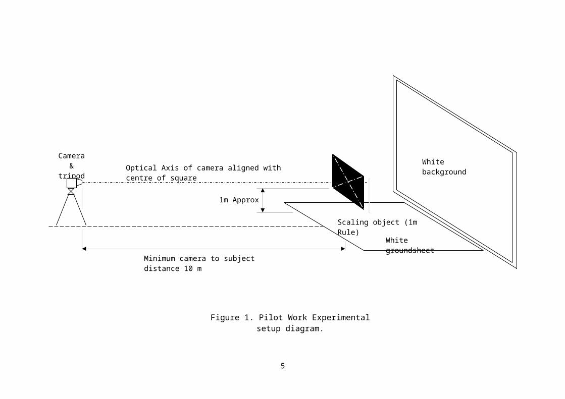
Figure 1. Pilot Work Experimental setup diagram.
Minimum camera to subject distance 10 m
Optical Axis of camera aligned with centre of squareWhite background
Camera & tripod
White groundsheet
Scaling object (1m Rule)
1m Approx
5

1.2. Data collection experimental setup
The experimental setup is shown in figure 2.
1.2.1. Camera position
Height – the centre of the lens was positioned at the same height as the top of the cycle
head tube.
Distance from subject – minimum horizontal distance of 8 m was observed between
the camera and the top of the cycle head tube. The scaling object was vertically
aligned with the top of the cycle head tube. The camera zoom facility was then be used
to select an appropriate image size. This process was performed in order to minimise
perspective error.
1.2.2. Subject position
The cycle was positioned first, separately to the subject, to allow proper camera/cycle
alignment. The camera was positioned in such a way that only the cycle in frontal
profile was observed with the front wheel totally obscuring the rear. Once the cycle
was correctly positioned, the subject positioned himself on the cycle in the desired
position.
6
1.2.3. Camera Setup
Camera used: Sony DSC-P9 4.0 Mega Pixel Digital Stills Camera.
Settings:
EV: OEV
Focus: Multi AF
White balance: Auto
Spot meter: On
ISO: Auto
Image size: 640 x 480
Picture quality: Fine
Record mode: Normal
Flash level: Normal
Picture effect: Off
7
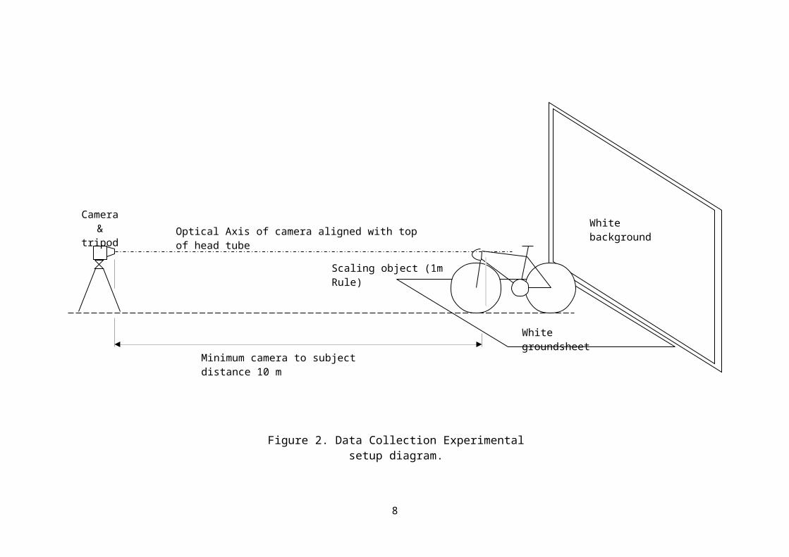
Optical Axis of camera aligned with top of head tubeWhite background
White groundsheet
Camera & tripod
Minimum camera to subject distance 10 m
Figure 2. Data Collection Experimental setup diagram.
Scaling object (1m Rule)
8
1.3. Pilot data collection
1.3.1. Measurement validity
By assessing measurement validity, we are answering the question “are we measuring what
we think we are measuring”, which in this case is FSA. In order to answer this question the
following pilot work was performed.
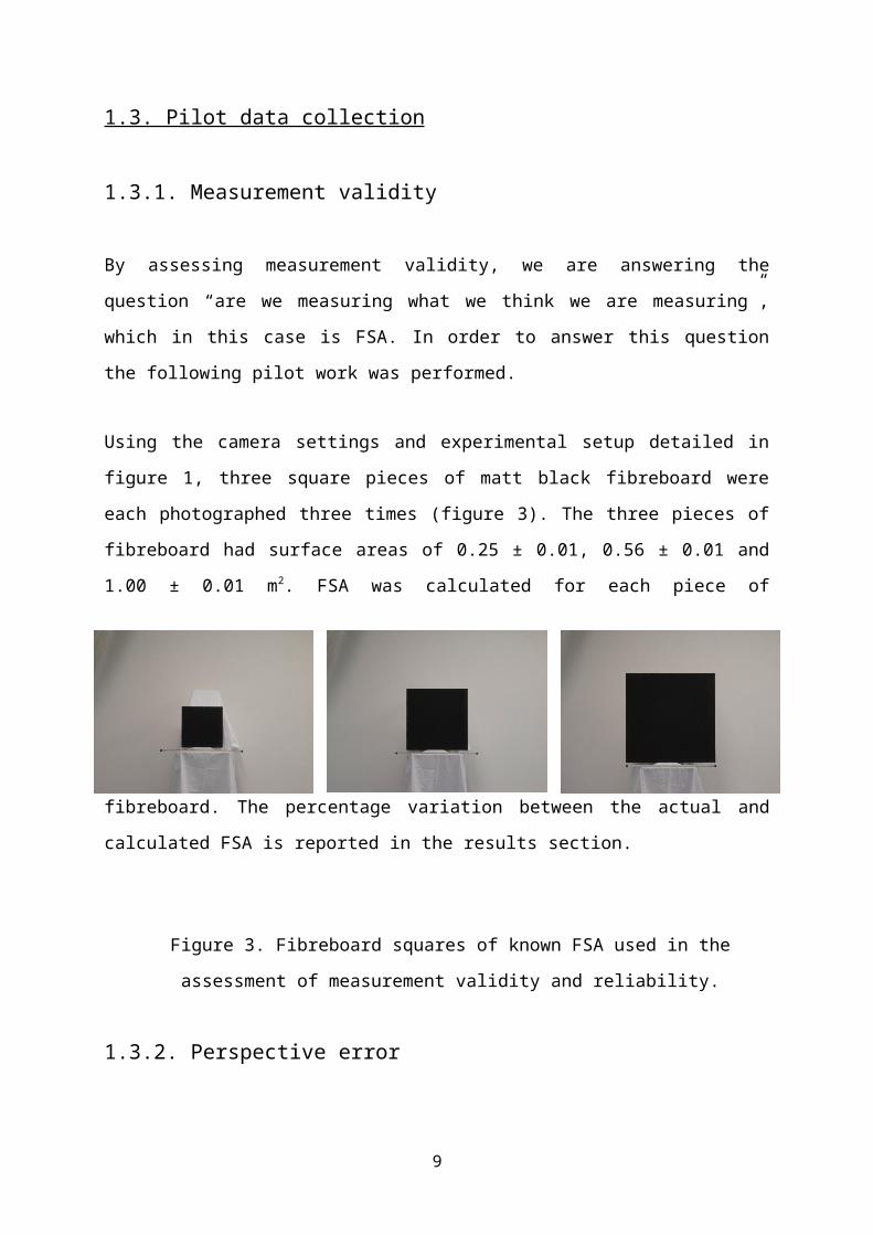
Using the camera settings and experimental setup detailed in figure 1, three square pieces of
matt black fibreboard were each photographed three times (figure 3). The three pieces of
fibreboard had surface areas of 0.25 ± 0.01, 0.56 ± 0.01 and 1.00 ± 0.01 m2. FSA was
calculated for each piece of fibreboard. The percentage variation between the actual and
calculated FSA is reported in the results section.
Figure 3. Fibreboard squares of known FSA used in the assessment of measurement
validity and reliability.
1.3.2. Perspective error
Perspective error occurs with deviation of the subject from the optical axis or focal plane of
the camera. The effect is incorrect information about the dimensions of objects or the special
relationship of objects i.e. objects closer to the camera can seem larger than they really are.
Using the camera settings and position detailed in figure 1, the 1 m2 fibreboard square was
photographed 0.5 m in front of and behind the scaling object. The variation of ± 0.5 m from
the scaling object was chosen as an approximation of the distances between the leading edge
9
of the front tyre and the scaling object and, the scaling object and the rider’s abdominal area.
The percentage variation between the actual and calculated FSA will be reported.
1.3.3. Measurement reliability
Measurement reliability concerns the accuracy of subsequent measurements using the same
method. In order to assess measurement reliability the following pilot work was performed.
Using the camera settings and position detailed in figure 1, the 1 m2 fibreboard shape was
photographed 10 times. Each time the setup was repeated as if a separate data collection
session were being performed. The FSA values were compared using the coefficient of
variation.
1.4. Results of pilot data collection
1.4.1. Measurement validity
Each of the fibreboard squares was measured with a metal rule (1 m), graded in 0.01 m
increments. The measured FSA area of the three squares was 0.25 ± 0.01, 0.56 ± 0.01 and 1 ±
0.01 m2. The mean FSA of the three fibreboard shapes calculated from the photographic
images analysed in the NIH image software was 0.25 ± 0.00, 0.56 ± 0.00 and 1 ± 0.00 m2. The
agreement between these vales suggests this is a valid method of assessing FSA. These results
are shown graphically in figure 4.
10
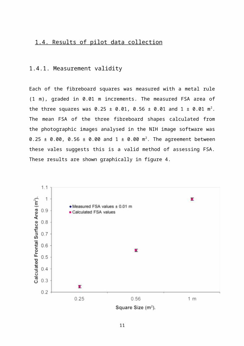
Figure 4. Comparison between the FSA of the three fibreboard squares measured with a 1 m
metal rule and FSA calculated using the method under validation.
1.4.2. Perspective error
The FSA of the 1 m2 fibreboard square was calculated to be 0.91 m with the board 0.5 m
behind the scaling object. With the 1 m2 fibreboard square 0.5 m in front of the scaling object,
the FSA was calculated to be 1.19 m. These values indicate a considerable variation in FSA
caused by variation in the position of the scaling object. The relationship between the position
of the scale object and the FSA of the 1 m2 fibreboard square can be explained by equations y
= 0.095x + 0.905 and y = -0.09x + 0.905 These equations relate to the scale object positioned
behind and in front of the 1 m2 fibreboard square respectfully.
11
1.4.3. Measurement reliability
The mean FSA of the 1 m2 fibreboard square photographed ten times was 0.99 ± 0.01 m2 The
coefficient of variation was 0.01 %. The agreement between the vales suggests this is a
reliable method of assessing FSA.
1.5. Sport specific pilot data collection
The pilot work detailed above provides an indication of the validity and reliability of this
method of calculating frontal surface area. In order to be sure that this method will produce
accurate and reliable FSA measurements when applied to the study of cyclists the following
sport specific pilot work was performed.
1.5.1. Assessment of three riding positions
A full data collection session was performed with a subject adopting three different riding
positions (figure 5): Bars – hands on the handlebars next to the stem, hoods – hands
positioned as if on the brake hoods, and drops – hands on the drop section of the handlebars.
The experimental and camera setup is shown in figure 2. Three photographs were taken of
each position
Figure 5. Three riding positions: Bars, Hoods and Drops.
12
1.5.2. Measurement reliability
Using the experimental setup detailed in figure 2, the subject was photographed 10 times.
Each time the setup was repeated as if a separate data collection session was being performed.
The subject was instructed to adopt the same position with hands on the handlebars next to the
stem. The FSA values were compared using the coefficient of variation.
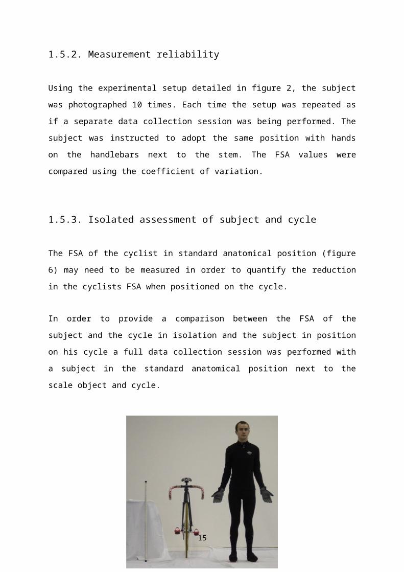
1.5.3. Isolated assessment of subject and cycle
The FSA of the cyclist in standard anatomical position (figure 6) may need to be measured in
order to quantify the reduction in the cyclists FSA when positioned on the cycle.
In order to provide a comparison between the FSA of the subject and the cycle in isolation
and the subject in position on his cycle a full data collection session was performed with a
subject in the standard anatomical position next to the scale object and cycle.
Figure 6. Subject in anatomical position next to cycle.
13

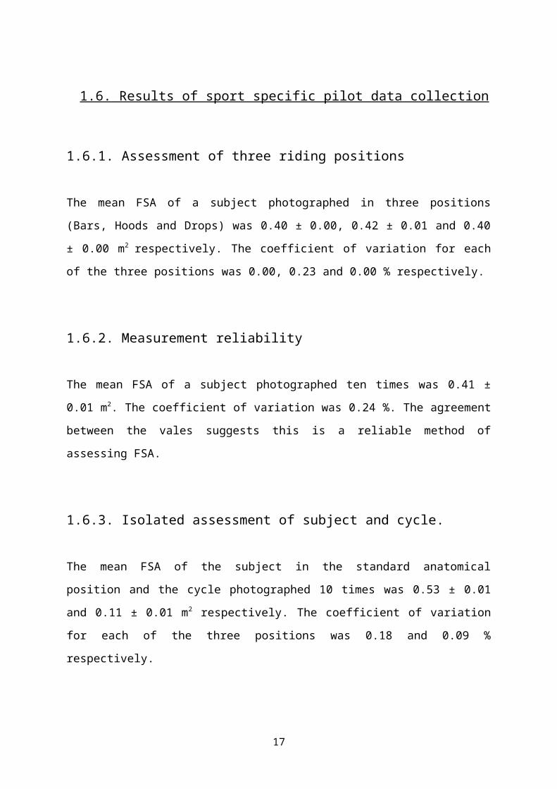
1.6. Results of sport specific pilot data collection
1.6.1. Assessment of three riding positions
The mean FSA of a subject photographed in three positions (Bars, Hoods and Drops) was
0.40 ± 0.00, 0.42 ± 0.01 and 0.40 ± 0.00 m2 respectively. The coefficient of variation for each
of the three positions was 0.00, 0.23 and 0.00 % respectively.
1.6.2. Measurement reliability
The mean FSA of a subject photographed ten times was 0.41 ± 0.01 m 2. The coefficient of
variation was 0.24 %. The agreement between the vales suggests this is a reliable method of
assessing FSA.
1.6.3. Isolated assessment of subject and cycle.
The mean FSA of the subject in the standard anatomical position and the cycle photographed
10 times was 0.53 ± 0.01 and 0.11 ± 0.01 m2 respectively. The coefficient of variation for
each of the three positions was 0.18 and 0.09 % respectively.
14
2. Data collection with Great Britain Endurance Squad
Photographs were taken of six members of the Great Britain endurance quad in the standard
anatomical position and in aerodynamic position on their cycles. The experimental setup
shown in figure 2 was used. Due to the colours of their clothing, the use of a white
aerodynamic helmet and white shoes, the photographs required blacking out manually before
thresholding (See Calculation of FSA) to distinguish the athletes from the white background.
Two measurements of FSA were made of each athlete in each of the two positions. The
results are shown in table 1. In order to quantify the repeatability of the measurements, the
FSA of a subject was calculated twelve times from one image. The mean FSA of the athlete
on his cycle in aerodynamic position was 0.33 ± 0.01 m2. The coefficient of variation for each
of the three positions was 0.03 % The agreement between the vales suggests this is a reliable
method of assessing FSA.
Table 1. Great Britain Endurance Squad mean FSA values
Athlete FSA values
Alteration to riding
positionAthlete on
bikeAthlete in
anatomical positionBike Athlete on bike Bike
(m2) (m2) (m2) (m2) (m2)
1 0.34 0 0.59 0.02 0.09 0.01
2 0.33 0.01 0.59 0 0.08 0.01
3 0.35 0 0.66 0.01 0.09 0.01
4 0.33 0 0.61 0.01 0.10 0.01
5 0.36 0.01 0.67 0.01 0.10 0
6 0.33 0.01 0.62 0.01 0.09 0 0.34 0.01 0.09 0
15

3. Guidelines for calculation of FSA from digital images
The following are specific guidelines for the manipulation of digital images in Adobe
Photoshop version 7 and the measurement of FSA in NIH image for Mac and Scionimage for
PC.
Section 1.2. (Data collection experimental setup) details the setup and positioning of the
camera and the subject. Figure 2 provides a visual reference for this setup.
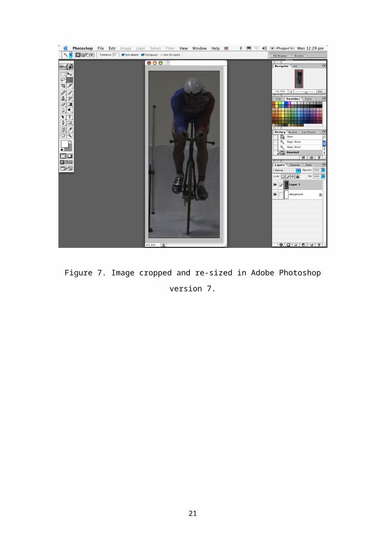
Import images to be used into Adobe Photoshop image software (version 7 is
recommended. The following guidelines are specific to this version), crop, and re-size
as appropriate using the Rectangular marquee and Crop tools in the Tools window
in the upper left hand corner of the screen. A cropped and re-sized image is shown in
figure 7.
Figure 7. Image cropped and re-sized in Adobe Photoshop version 7.
16
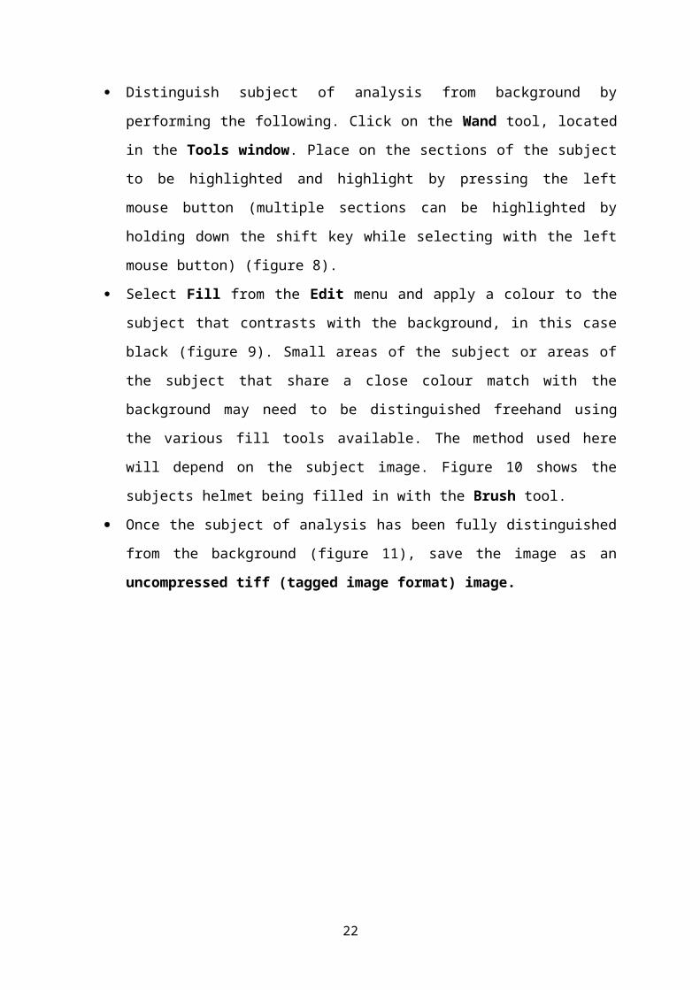
Distinguish subject of analysis from background by performing the following. Click
on the Wand tool, located in the Tools window. Place on the sections of the subject to
be highlighted and highlight by pressing the left mouse button (multiple sections can
be highlighted by holding down the shift key while selecting with the left mouse
button) (figure 8).
Select Fill from the Edit menu and apply a colour to the subject that contrasts with the
background, in this case black (figure 9). Small areas of the subject or areas of the
subject that share a close colour match with the background may need to be
distinguished freehand using the various fill tools available. The method used here
will depend on the subject image. Figure 10 shows the subjects helmet being filled in
with the Brush tool.
Once the subject of analysis has been fully distinguished from the background (figure
11), save the image as an uncompressed tiff (tagged image format) image.
Figure 8. Multiple sections of subject image highlighted ready for filling.
17
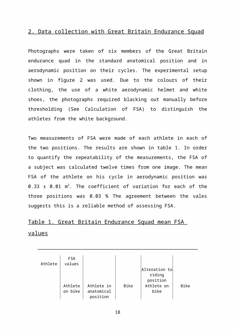
Figure 9. Colour determination using the fill window.
Figure 10. Continued “freehand” filling of subject image using the brush tool.
18

Figure 11. Completed subject image filled to provide contrast to background colour.
19
Import images into NIH image software if using a Mac (figure 12), or Scionimage
software if using a PC.
Figure 12. Image imported into NIH image.
20
Ensure the LUT window is white at the top moving to black at the bottom. If this is
not the case, select Greyscale from the Options menu. Then select Invert from the
Edit menu.
Using the Straight-line tool located in the Tools window (5th tool from the top, right
hand side), draw a line across the scale object (figure 13). Go to the Analyse menu
and choose Set Scale. Choose the Units of measure first then enter the Known
Distance (if the scale object used is 1 m long, the Units would be Meter and the
Known Distance would be 1). Click the OK button to continue.
Figure 13. Setting the scale.
21
Select Threshold from the Options menu. This should remove the background
leaving the subject clearly separate from the background. Adjust the threshold in the
LUT window to ensure the subject is fully separated from the background by placing
the mouse at the junction between black and white, holding down the left mouse
button and moving the threshold up or down.
Using the Wand tool, (9th tool from the top, left hand side), click to the left of the
subject. This should draw a border around the subject. Choose Measure from the
Analyse menu. The FSA value will appear in the Info window located in the bottom
left hand corner of the desktop (Figure 14).
Figure 14. Thresholding and FSA measurement.
22