CAFixD – A CASE-BASED REASONING METHOD FOR FIXTURE …

CAFixD – A CASE-BASED REASONING METHOD FOR FIXTURE DESIGN

by Iain Boyle

A PhD dissertation

Submitted to the Faculty of the

WORCESTER POLYTECHNIC INSTITUTE in partial fulfilment of the requirements for the

Degree of Doctor of Philosophy in

Manufacturing Engineering by

---------------------------------------------------

May 2006

APPROVED: ------------------------------------------------------ Professor Yiming (Kevin) Rong, Advisor, Professor of Mechanical Engineering ------------------------------------------------------ Professor David C. Brown, Co-advisor, Professor of Computer Science

------------------------------------------------------ Professor Yiming (Kevin) Rong, Professor of Mechanical Engineering, Associate Director of Manufacturing and Materials Engineering Program

��

��

Fixtures accurately locate and secure a part during machining operations such that the part can be manufactured to design specifications. To reduce the design costs associated

with fixturing, various computer-aided fixture design (CAFD) methods have been developed through the years to assist the fixture designer. Much research has been directed towards developing systems that determine an optimal fixture plan layout, but

there is still a need to develop a CAFD method that can continue to assist designers at the unit level where the key task is identifying the appropriate structure that the individual

units comprising a fixture should take. This research work details the development of a CAFD methodology (called CAFixD) that seeks to fill this hole in the CAFD field. The

approach taken is to consider all operational requirements of a fixture problem, and use them to guide the design of a fixture at the unit level. Based upon a case-based reasoning

(CBR) methodology where relevant design experience is retrieved and adapted to provide a new fixture design solution, the CAFixD methodology adopts a rigorous approach to

indexing design cases in which axiomatic design functional requirement decomposition is adopted. Thus, the design requirement is decomposed in terms of functional

requirements, physical solutions are retrieved and adapted for each individual requirement, and the design re-constituted to form a complete fixture design. Case

adaptation knowledge is used to guide the retrieval process. Possible adaptation strategies for modifying candidate cases are identified and then evaluated. Case and adaptation

strategy combinations that result in adapted designs that best satisfy the preferences of the designer are used as the final design solutions. Possible means of refining the

effectiveness of the method include combining adaptation strategies and considering the order in which design decisions are taken.

Keywords: axiomatic design, case-based reasoning, fixture design, retrieval-by-

adaptability.

��

� � � ��

The author would like to thank the following individuals for their contribution throughout this project:

Professor Yiming (Kevin) Rong (dissertation advisor) for offering the author an opportunity to conduct this research at WPI, and for the guidance, encouragement and

suggestions he has provided throughout its duration;

Professor David C. Brown (co-advisor) for his willingness to provide extensive advice and feedback;

Professor Chris Brown, Professor Richard D. Sisson, and Professor Yong-Mo Moon for

their commitment demonstrated as members of the author’s dissertation committee;

Members of the CAMLAB for their help in developing the CAFixD system;

Professor Yiming (Kevin) Rong, the Mechanical Engineering Department at WPI, and the Provost’s Office/Division of Academic Affairs for graciously funding this period of

study.

��

��

�� _______________________________________________________________ i � � � �� ____________________________________________________ ii �� ______________________________________________________ iii �� _________________________________________________________ vi �� __________________________________________________________ ix �� _________________________________________________ 1

�� ________________________________________________ 2 ��!�� "� �� !�� "� �� !�� "� �� !�� "� �� __________________________________________________________ 5 ��#�$� ��%� �� #�$� ��%� �� #�$� ��%� �� #�$� ��%� �� ______________________________________________________________ 9 ��&�'� �� ( � )� ��%� ��&�'� �� ( � )� ��%� ��&�'� �� ( � )� ��%� ��&�'� �� ( � )� ��%� � ___________________________________________________ 12 ��*�"�� *�"�� *�"�� *�"�� ___________________________________________________ 13

�� !�� !�� !�� !�� '� %�� '� %�� '� %�� '� %�� ___________________________________________ 14 !�� !�� !�� !�� ++++� �� "� �� "� �� "� �� "� �� __________________________________________ 14

!��'� �� "�� , ___________________________________________14 !��!��- � � �� " __________________________________________________________26

!��!�� ______________________________________________________26 !��!�!�"� �� . � , �� "� �� / � �� ___________________________31 !��!�#�/ � � � �� / �� '� - � �� "� �� "� �� . �� __35

!�!�� !�!�� !�!�� !�!�� ++++� � �� '� � �� '� � �� '� � �� '� � �� _________________________________________________ 38 !�!�� __________________________________________________________________41 !�!�!�'� �� %� � _________________________________________________________________50

!�!�!�� , +� � �� '� �� %� �_______________________________________________50 !�!�!�!�� , +� � �� '� �� %� �_____________________________________________51

!�#�� "� �� !�#�� "� �� !�#�� "� �� !�#�� "� �� ______________________________________________________ 57 !�&�"� �� !�&�"� �� !�&�"� �� !�&�"� �� ++++� � �� "� �� / �� / ��, �� , ��0"1 "/ / �2� � �� "� �� / �� / ��, �� , ��0"1 "/ / �2� � �� "� �� / �� / ��, �� , ��0"1 "/ / �2� � �� "� �� / �� / ��, �� , ��0"1 "/ / �2 ____________________ 64 !�*�� ,!�*�� ,!�*�� ,!�*�� , _____________________________________________________________ 69

�� #�� #�� #�� #��'� �� ( � )� ��%� �� $� �� ,�'� �� ( � )� ��%� �� $� �� ,�'� �� ( � )� ��%� �� $� �� ,�'� �� ( � )� ��%� �� $� �� , ________________________ 70 #��'� �� ( � )� ��%� �#��'� �� ( � )� ��%� �#��'� �� ( � )� ��%� �#��'� �� ( � )� ��%� � ___________________________________________________ 70 #�!�. �� #�!�. �� #�!�. �� #�!�. �� ____________________________________________________ 73

�� &�� &�� &�� &��. �� "� �� $� �� ,�. �� "� �� $� �� ,�. �� "� �� $� �� ,�. �� "� �� $� �� , _______________________________ 76 &�� "�( %� �%�� &�� "�( %� �%�� &�� "�( %� �%�� &�� "�( %� �%�� ______________________________________________________ 76 &�!�� "� �� &�!�� "� �� &�!�� "� �� &�!�� "� �� _________________________________________________ 80

&�!�� "� �� __________________________________________________81 &�!�!�� , �� ____________________________________________________________82 &�!�#�� '�"� � � � � �� _________________________________________________________88

&�!�#�� '� �� '�"� � � � � �� _____________________93 &�!�#�� '�� _________________________________________94 &�!�#��!�� '�� ! _________________________100

�%�

&�!�&�� "� � � � � �� , �!________________________________________116 &�!�*�� $� � � � �� ______________________________________________________125

&�#�'� �� %� �� &�#�'� �� %� �� &�#�'� �� %� �� &�#�'� �� %� �� , �!, �!, �!, �! ___________________________________________ 128 &�#�� , +� � �� '� �� %� ��03 � �� "� �� 2 ___________________129 &�#�!�� , +� � �� '� �� %� �________________________________________________131

&�#�!��. �� / ��, �� , �� ___________________________________________132 &�#�!��"� �� 4 �� '� � � � �______132 &�#�!��!�4 � � � �� / ��, �� %� � __________________________________________133 &�#�!��#�"� �� 5� � ____________________138

&�#�#�6%� �� "�� "� �� ___________________141 &�#�#��4 � � � �� "� �� ____________________________________________142 &�#�#�!�� "� �� "� �� , +� � �� '� �� %� � _____________________144

&�#�#�!�� _____________________________________________148 &�#�#�!��$� � �� $� � � �� __________________________________________150

&�#�#�!��$� � ��, �� 5�7 � � 5�� 6�� __________157 &�#�#�!��!�$� � ��, �� 1 � � � �6�� ______________________________162 &�#�#�!��#�$� � ��, �� 6�� ____________________________165

&�#�#�!��!�� $� � �� "� �� _____________________________________167 &�#�#�!��#�� , ______________________________176

&�#�#�!�!�6%� �� "�� ". 8�� , �� _____________181 &�&�'� %�� &�&�'� %�� &�&�'� %�� &�&�'� %�� ______________________________________________________________ 189

�� *�� *�� *�� *��7 � � � � �6 � � � �� 7 � � � � �6 � � � �� 7 � � � � �6 � � � �� 7 � � � � �6 � � � �� _________________________________________ 190 *�� 6 � � � ��*�� 6 � � � ��*�� 6 � � � ��*�� 6 � � � �� _____________________________________________________ 190 *�!�( � � �� 6 � � � ��*�!�( � � �� 6 � � � ��*�!�( � � �� 6 � � � ��*�!�( � � �� 6 � � � �� ____________________________________________________ 193

*�!��"� �� $� � � � ____________________________________________194 *�!�!�� '�� ________________________________________________201 *�!�#�'� �� %�� / � �� , �!_________________________________216

*�#�'� %�� *�#�'� %�� *�#�'� %�� *�#�'� %�� ______________________________________________________________ 231 �� 9�� 9�� 9�� 9��, �� "� %� �� , �� "� %� �� , �� "� %� �� , �� "� %� �� ____________________ 233

9��, �� ( %� �%�� 9��, �� ( %� �%�� 9��, �� ( %� �%�� 9��, �� ( %� �%�� _____________________________________________________ 233 9�!��, �� "� �� 9�!��, �� "� �� 9�!��, �� "� �� 9�!��, �� "� �� ____________________________________________________ 235 9�#�� 9�#�� 9�#�� 9�#�� _____________________________________________________ 239

9�#��. �� "� �� 4 � � � �� ___________________________________239 9�#�!�. �� !��4 � � � �� / ��, �� %� �� ____________________240 9�#�#�. �� #��'� �� %� � ______________________________________________________240 9�#�&�. �� &��"� �� $� � �� +� � �� $� �� ___________________242

9�&�"� �� 9�&�"� �� 9�&�"� �� 9�&�"� �� _______________________________________ 245 9�&��"� �� 7 � � � �� "��, �� ______________246 9�&�!�"� �� $� � �� . . ��, �� _____________248 9�&�#�"� �� "� �� "��, �� ___________248 9�&�&�"� �� $� � �� . � �� "��, �� ______________________249

9�*��, ��9�*��, ��9�*��, ��9�*��, �� ______________________________________________________ 251 :�� :�� :�� :�� _______________________________________________________ 255

:�� :�� :�� :�� _________________________________________________________ 255 :�!�6%�:�!�6%�:�!�6%�:�!�6%� �� ____________________________________________________________ 258 :�#�� 7 � �:�#�� 7 � �:�#�� 7 � �:�#�� 7 � � __________________________________________________________ 271

%�

'� �� '� �� '� �� '� �� _________________________________________________________ 273 �� '8"�� '8"�� '8"�� '8". �� . �� #. �� . �� #. �� . �� #. �� . �� #++++!!!!++++�� 3 � �� #�� 3 � �� #�� 3 � �� #�� 3 � �� # _________ 282 �� 1 �� 1 �� 1 �� 1 �� , �!�� , �!�� , �!�� , �!___________________________ 290 �� 7 � � � �� 4 � ��7 � � � �� 4 � ��7 � � � �� 4 � ��7 � � � �� 4 � � � � ��,� � ��,� � ��,� � ��, _____________________________________ 304 �� "�� "�� "�� "�� '8". �� 0� '�� !2�� '8". �� 0� '�� !2�� '8". �� 0� '�� !2�� '8". �� 0� '�� !2 __________________ 306 �� 6�� 6�� 6�� 6�� . � �� 3 � �� 6 �� . � �� 3 � �� 6 �� . � �� 3 � �� 6 �� . � �� 3 � �� 6 �� ___ 311 �� "�� / � � � �� "�� / � � � �� "�� / � � � �� "�� / � � � �� ______________________________ 312 �� 4 �� 4 �� 4 �� 4 ��7 � � � �� 7 � � � �� 7 � � � �� 7 � � � �� _______________________________________ 314 �� ; �� ; �� ; �� ; ��$� � �� $� � �� $� � �� $� � �� _______________________________________ 315 �� $� � �� $� � �� $� � �� $� � �� ___________________________ 316

%��

��

Figure 1: A typical modular fixture, shown a) without and b) with a workpiece (Rong, 1999)___________3 Figure 2: The basic elements of the fixture design process (Kang et al., 2003) ______________________6 Figure 3: The six degrees of freedom_______________________________________________________8 Figure 4: The standard 3-2-1 locating model ________________________________________________8 Figure 5: A support unit with recommended dimension relations ________________________________17 Figure 6: A workpiece and its datum machining surface relationship graph (Hu, 2001) ______________19 Figure 7: A vertical locating unit_________________________________________________________20 Figure 8: Possible ways of fixing a design__________________________________________________28 Figure 9: Modifying a horizontal locating unit ______________________________________________29 Figure 10: A pin array type fixture (Hurtado & Melkote, 2001) _________________________________32 Figure 11: L-shaped locators____________________________________________________________34 Figure 12: The CBR process (Maher, 1997) ________________________________________________40 Figure 13: The decomposition of case recall and adaptation (Maher, 1997) _______________________41 Figure 14: Identifying the critical tolerances _______________________________________________46 Figure 15: Two workpieces _____________________________________________________________48 Figure 16: Caliper locating surfaces ______________________________________________________48 Figure 17: Limitations of linear based weighting ____________________________________________51 Figure 18: Limitations with attribute-based retrieval _________________________________________52 Figure 19: Comparing two cases with the same tolerance capability _____________________________54 Figure 20: Axiomatic design domains (Suh, 2001) ___________________________________________58 Figure 21: A sample probability density function (Suh, 2001) __________________________________60 Figure 22: pdfs for a) construction cost/time and b) slope stability (Pena-Mora & Li, 2001) __________62 Figure 23: Tightening the design range____________________________________________________63 Figure 24: A Utility Curve ______________________________________________________________64 Figure 25: Expressing a designer's preferences _____________________________________________65 Figure 26: Determining the Overall Utility of a Design Case ___________________________________66 Figure 27: An example of a lottery question ________________________________________________67 Figure 28: The Effect of a High Number of Attributes Upon Calculated Utility _____________________68 Figure 29: The fixture design methodology _________________________________________________77 Figure 30: Axiomatic design domains applied to fixture design _________________________________80 Figure 31: The design case base _________________________________________________________82 Figure 32: Case library 1 - conceptual design solutions (Rong, 1999) ____________________________83 Figure 33: Decomposition of conceptual 3-2-1 locating solutions _______________________________84 Figure 34: An interfering surface between locating points _____________________________________86 Figure 35: A redundant common locating unit ______________________________________________87 Figure 36: A partial FR skeleton set for 3-2-1 plane locating, variation 3 _________________________89 Figure 37: The matching design parameters for the partial FR skeleton set________________________90 Figure 38: A clamping unit with chip shedding ability ________________________________________92 Figure 39: Determining the primary locating direction________________________________________96 Figure 40: True position, parallel, and perpendicular tolerance specifications _____________________95 Figure 41: Choosing locating faces _______________________________________________________98 Figure 42: Determining how equilateral a triangle is _________________________________________99 Figure 43: Updating the FR and DP skeleton sets (sample values only)__________________________100 Figure 44: Definition of true position tolerance (ASME,1994) _________________________________101 Figure 45: a) Perpendicular and b) parallel tolerance definitions (ASME,1994)___________________102 Figure 46: Performing the sensitivity analysis______________________________________________103 Figure 47: Performing a sensitivity analysis for a parallel tolerance ____________________________105 Figure 48: Effect of varying an angle upon shift of interest____________________________________108 Figure 49: Calculating the tolerance allowed at each locating position__________________________108 Figure 50: Design tolerances dependent upon several locating point pairs _______________________109 Figure 51: Completing FR1 ____________________________________________________________112 Figure 52: Changes in locating positions caused by workpiece rotations_________________________113

%��

Figure 53: Completing FR2 (sample values only) ___________________________________________116 Figure 54: The high level view of case library 2 ____________________________________________117 Figure 55: The decomposition of locating units in case library 2 _______________________________118 Figure 56: The Two Types of Horizontal Locators, HL01 and HL02 ____________________________119 Figure 57: The Different Types of Horizontal Locating_______________________________________119 Figure 58: Integrated and assembled locating units _________________________________________120 Figure 59: The decomposition of clamping units in case library 2 ______________________________121 Figure 60: The three strap clamp lever classes _____________________________________________122 Figure 61: A third order vertical clamp and its equivalent element sketch ________________________124 Figure 62: The library maintenance mechanism ____________________________________________127 Figure 63: Functional and behavioural split within the locating unit section of case library 1 ________130 Figure 64: A sample of possible utility curve shapes_________________________________________134 Figure 65: A sample lottery question _____________________________________________________135 Figure 66: Generating a utility curve ____________________________________________________135 Figure 67: Creating a utility curve for cost ________________________________________________136 Figure 68: Lottery question used to determine the cost utility curve _____________________________136 Figure 69: Updating the cost constraint utility curve ________________________________________137 Figure 70: The completed utility curve for the cost constraint attribute __________________________138 Figure 71: Lottery question used to determine the scaling constant for cost_______________________140 Figure 72: A sample list of FRs and possible DP solutions____________________________________143 Figure 73: Part of the schema for a vertical clamp __________________________________________144 Figure 74: The adaptation mapping layout ________________________________________________145 Figure 75: Local constraint limiting a dimensional change ___________________________________148 Figure 76: Pseudo code representation of selecting adaptation strategies ________________________149 Figure 77: A third order vertical strap clamp and its element skeleton___________________________151 Figure 78: Thickness changes on a third order vertical strap clamp ____________________________151 Figure 79: Width changes on a third order vertical strap clamp________________________________152 Figure 80: Start and end thicknesses for a) rectangular and b) circular cross sections ______________157 Figure 81: The forces in a lever arrangement ______________________________________________157 Figure 82: A standard fulcrum layout ____________________________________________________158 Figure 83: Altering the length of a fulcrum element _________________________________________159 Figure 84: Modifying fulcrum components ________________________________________________161 Figure 85: Collisions between contact, fulcrum, and work limbs _______________________________161 Figure 86: Splitting up the strap beam (side projection view)__________________________________162 Figure 87: Modelling the strap beam (plan view) ___________________________________________163 Figure 88: Modifying elements within elem2 (side projection view) _____________________________164 Figure 89: Modifying elements within the beam due to thickness increases of the work elements ______165 Figure 90: Mating conventions in CAFixD ________________________________________________166 Figure 91: Modifying connection properties on a fulcrum element (cross sectional view) ____________167 Figure 92: The displacment analysis for a clamping unit _____________________________________168 Figure 93: Boundary conditions for the unit stiffness analysis _________________________________171 Figure 94: The virtual force system ______________________________________________________172 Figure 95: Obtaining the internal forces for the real system___________________________________172 Figure 96: Splitting up the beam ________________________________________________________174 Figure 97: Equilibrium solutions for elem2________________________________________________174 Figure 98: Equilibrium solutions for elem1________________________________________________175 Figure 99: Calculating dwork for element i _________________________________________________176 Figure 100: Flow diagram of dimensional change control module______________________________178 Figure 101: The material_control() module _______________________________________________181 Figure 102: An assumed accuracy cost function ____________________________________________183 Figure 103: Updating the adaptation mapping layout to include U(X) ___________________________186 Figure 104: A vertical clamping unit_____________________________________________________191 Figure 105: The workpiece and design tolerances __________________________________________195 Figure 106: The DMSRG for the workpiece _______________________________________________196 Figure 107: Evaluating the use of surface 1 for locating point P3 ______________________________198 Figure 108: Maximising the locating area_________________________________________________199

%��

Figure 109: The locating point distribution of conceptual design _______________________________200 Figure 110: The updated FR/DP skeletons upon completion of setup and fixture planning ___________201 Figure 111: Analyzing the workpiece tolerances____________________________________________202 Figure 112: Using the x coordinate of locating point P2 instead of P3 during the sensitivity analysis __205 Figure 113: The perpendicular tolerance on hole 18 ________________________________________206 Figure 114: The allowed design tolerance on hole 18________________________________________206 Figure 115: Determining TolP1 and TolP2 _________________________________________________208 Figure 116: Maximum machining forces acting against each locating direction ___________________213 Figure 117: Obtaining a clamping position to act against locating point P2 ______________________214 Figure 118: Utility curve for fixture cost __________________________________________________217 Figure 119: Utility curve for weight _____________________________________________________217 Figure 120: Utility curve for loading time_________________________________________________218 Figure 121: Utility curve for assembly time________________________________________________218 Figure 122: Utility curve for unloading time_______________________________________________219 Figure 123: Element 4 a) before and b) after modification ____________________________________223 Figure 124: Calculating Ff and Fw_______________________________________________________224 Figure 125: Free body diagram for element 4______________________________________________224 Figure 126: Limitations on modifying the work and fulcrum limbs______________________________228 Figure 127: The adaptation mapping layout for this FR/DP combination ________________________231 Figure 128: CAFixD system overview ____________________________________________________234 Figure 129: Databases that support CAFixD operation ______________________________________236 Figure 130: Modifying a utility curve ____________________________________________________237 Figure 131: The domain knowledge database ______________________________________________238 Figure 132: Generating a conceptual design_______________________________________________241 Figure 133: Generating utility curves and scaling constants __________________________________243 Figure 134: Retrieval based upon functional similarity_______________________________________244 Figure 135: Modification and case-base maintenance _______________________________________245 Figure 136: The geometric data of a rectangular plane ______________________________________247 Figure 137: The geometric data of a hole _________________________________________________247 Figure 138: Element 10 before modifications ______________________________________________250 Figure 139: Element 10 after modifications _______________________________________________251 Figure 140: The main CAFixD Screen____________________________________________________253 Figure 141: The case library status ______________________________________________________254 Figure 142: A vertical locating unit______________________________________________________259 Figure 143: Utility curves for attributes 1, 2, and 3 _________________________________________261

� �

��

Table 1: Summary of CAFD research focus_________________________________________________15 Table 2: Design considerations incorporated into previous CAFD research efforts__________________37 Table 3: Kumar & Nee (1995) Indexing Attributes ___________________________________________44 Table 4: Design datums and multiple setup planning _________________________________________96 Table 5: The sensitivity analysis table ____________________________________________________103 Table 6: The allowed variations, �, at each locating point ____________________________________106 Table 7: Updating the tolerance table to show all contributory factors __________________________111 Table 8: A schema for a clamping unit ___________________________________________________123 Table 9: A schema for an individual clamping unit element ___________________________________124 Table 10: The acceptable performance ranges for each constraint attribute ______________________139 Table 11: A schema for a clamping unit __________________________________________________153 Table 12: A schema for an individual clamping element ______________________________________154 Table 13: Internal virtual work equations for shear, axial, and bending moment loads (Hibbeler, 1997) 169 Table 14: Refining the dimension change _________________________________________________179 Table 15: Results using standard utility analysis for high numbers of attributes ___________________188 Table 16: Employing the grouping method for design 1 ______________________________________188 Table 17: The completed schema for the clamping unit_______________________________________192 Table 18: Completed element schema for element 4 _________________________________________193 Table 19: The machining information ____________________________________________________196 Table 20: Tabular format of DMSRG ____________________________________________________196 Table 21: Orientation of normals for each machined feature __________________________________197 Table 22: Refining the selection of primary, secondary, and tertiary locating directions_____________197 Table 23: Determining the optimum position for P2 _________________________________________199 Table 24: The conceptual design details __________________________________________________200 Table 25: The sensitivity of feature 7 to variations in locating pair P1 and P2_____________________203 Table 26: Updating the sensitivity table___________________________________________________204 Table 27: The final sensitivity analysis table _______________________________________________204 Table 28: Updating the tolerance table ___________________________________________________209 Table 29: The allowed tolerance, �, of each locating point (inches)_____________________________211 Table 30: The tolerance assignments for each locating point (inches) ___________________________212 Table 31: Summary of machining and clamping forces acting against each locator_________________213 Table 32: The required stiffness at each locating and clamping point ___________________________214 Table 33: Clamping orientations and positions _____________________________________________215 Table 34: Individual scaling constants ki and overall scaling constant K _________________________219 Table 35: Output of results from functional similarity-based retrieval ___________________________220 Table 36: Attribute performance values for initial design _____________________________________221 Table 37: Modification results for strap_thickness_adapt() strategy (inches)______________________225 Table 38: The updated constraint attributes for the clamp ____________________________________226 Table 39: The updated attribute performance values for the modified fixture______________________226 Table 40: Testing results for the alter_width() modification module (inches) ______________________227 Table 41: Displacment results for different materials ________________________________________228 Table 42: The updated constraint attributes for the clamp ____________________________________228 Table 43: The updated attribute performance values for the modified fixture______________________229 Table 44: Comparison of the utility of each adaptation strategy________________________________229 Table 45: The modification list for element 10______________________________________________250 Table 46: Material properties __________________________________________________________259 Table 47: Results gained by implementing the adaptation strategies ____________________________260 Table 48: Contributions of designs A and B to attributes 1, 2, and 3 ____________________________261 Table 49: Design state 1 analysis________________________________________________________262 Table 50: Design state 2 analysis________________________________________________________262

��

��

A key concern for a manufacturing company is the ability to design and produce a variety of high quality products in as short a time as possible. Quick release of a new product

into the market place, ahead of any competitors, is a crucial factor in being able to secure a higher percentage of the market place and a higher profit margin. As a result of the consumer desire for variety, batch production of products is now more the norm than

mass production, which has resulted in the need for manufacturers to develop flexible, agile manufacturing practices to achieve a rapid turnaround in product development.

A key aspect of developing a product is the design stage in which ideas for a product

must be generated and evaluated. This can be a lengthy, complex, and often iterative affair involving many phases such as:

• identifying the need for a product;

• generating initial ideas for a potential solution;

• evaluating these ideas;

• refining them and adding greater levels of detail;

• testing them for the purposes of further evaluation;

• producing complete specifications for the chosen solution;

• preparing all necessary documentation such as manufacturing drawings and

materials listings.

Not only must the product itself be designed, but so too must the means by which it will be produced. Thus all the above steps must be repeated to design a suitable production

setup. Obviously therefore the financial costs and time delays that can accrue during the design of both the product and the manufacturing set up can be detrimental to a

company’s ability to meet the demands of the marketplace

!�

Over the past twenty years or so, computers have been employed more and more to assist these activities. Computer-aided design (CAD) and computer-aided manufacturing

(CAM) systems are used to aid design and manufacturing tasks, with the objective of reducing the duration and costs of these steps in the production process. Many systems

have been developed to provide assistance with particular aspects of the design and manufacturing stages. During design, for example, CAD systems can predict the expected

behaviour of designs, assist the designer during decision making processes, and help rapidly evaluate different designs. During manufacture, CAM systems can assist with

aspects such as planning, data communication, material requirement planning, and generating of machine tool cutting paths, to name but a few.

Such computer tools are used to support many parts of the production process. One

important component within production is fixturing. Whilst undergoing many of the operations that form part of its manufacturing process, a product must be held securely in

position. A fixture is a special tool used to rapidly and accurately position (or “locate” as is the more commonly used term) the workpiece, and support and secure it adequately

such that all parts that are produced using this fixture will be within the design specifications for that part. This accuracy facilitates the interchangeability of parts that is

prevalent in much of modern manufacturing. There are many types of manufacturing operations such as various forms of heat treatment, welding, chemical treatments, and so

on. For the purposes of this dissertation the focus will be on fixtures used in machining processes such as milling and drilling, in which, the accuracy of location is measured

relative to the position of the machine tool performing the machining operation.

��

Physically a fixture is comprised of devices capable of supporting and clamping the workpiece (Rong, 1999). There are many means of achieving this, ranging from simple

vice grips or lathe chucks to more unusual fixtures that are based upon phase change materials in which the physical property (such as temperature or pressure) of a certain

#�

material is manipulated to initially change the material’s phase from liquid to solid in order to locate and secure the workpiece, before being altered again to allow the material

to revert back to a liquid form from which the workpiece can be removed. For the purposes of this dissertation however more conventional fixtures such as that illustrated

in Figure 1 will be studied.

Figure 1: A typical modular fixture, shown a) without and b) with a workpiece (Rong, 1999)

In such typical fixtures the workpiece rests on locators that accurately locate the

workpiece. Clamps are used to hold the workpiece against the locators during machining thus securing the workpiece’s location. The typical structure of a fixture consists of a

base-plate, to which the clamping and locating units are attached. The locating units

&�

themselves consist of the locator supporting unit and the actual locator. The locator is the part of the locating unit that contacts the workpiece. The clamping units consist of a

clamp supporting unit and a clamp that actually contacts the workpiece and exerts a clamping force on it. Fixtures may contain different numbers and different types of

clamping and locating units, but units generally always follow the same basic format that consists of a supporting unit upon which sits a particular type of locator or clamp.

Although the primary function of a fixture is to accurately locate and secure a workpiece,

there are many other criteria that it should attempt to satisfy, most often concerned with ergonomic factors. These may include that the fixture should be:

• be simple and quick to operate (by facilitating easy loading and unloading of the

workpiece from the fixture);

• be error-proof (prevent the workpiece from being loaded into the fixture

incorrectly orientated);

• offer some means of preventing unnecessary chip accumulation during machining;

• provide extra support where necessary for unusually shaped or large workpieces;

• offer some means of guiding the tool onto the workpiece (fixtures that have this

particular feature are often referred to as jigs).

Finally one of the most important aspects of a fixture is that it should not add

unnecessarily to production costs, whether the cost is incurred as a result of fixture assembly time, expensive materials, fixture manufacture costs, and so on.

A further aspect related to fixture design is that different design considerations often

conflict with each other. For example a heavy fixture can be advantageous as this aids the stability of the fixture. However increasing the weight of a fixture can have an adverse effect upon cost due to the increase of material costs that this would incur and also

because the fixture would become more difficult to handle as a result of its weight. All of

*�

these considerations contribute therefore to making the fixture design process a complex one.

Fixtures have a direct effect upon machining quality, productivity, and the cost of

products. Indeed, the costs associated with fixture design and manufacture can account for 10 – 20% of the total cost of a manufacturing system (Bi & Zhang, 2001). These costs

relate not only to the material costs of the fixture and the labour involved in assembling and operating them, but also to the cost of designing these fixtures. Hence there are

significant benefits to be reaped by reducing the design costs associated with fixturing.

There are two approaches that have been pursued with this aim. One has concentrated on developing flexible fixture systems, the other on simplifying the design process. The

most prominent example of the former approach is the development of modular fixture systems. These systems consist of a set of standard fixture components that can be

connected together in a variety of configurations to produce a large range of fixtures from a fixed number of individual components. Other, though lesser used flexible fixturing

techniques include the use of phase-changing materials to hold workpieces in place (Hazen & Wright, 1990), programmable fixtures (Tuffentsammer, 1981), and adjustable

fixtures (Zhu & Zhang, 1990; Jiang et al., 1988). However, the significant limitation of the flexible fixturing mantra is that it does not address the difficulty of designing fixtures.

To combat this problem, an alternative approach adopted to reduce fixturing costs has been to simplify the fixture design process.

��!�� "� �� !�� "� �� !�� "� �� !�� "� ��

Various computer-aided fixture design (CAFD) systems, normally employing artificial

intelligence techniques, have been developed through the years to assist the designer during the various stages of fixture design (see Figure 2).

9�

Figure 2: The basic elements of the fixture design process (Kang et al., 2003)

There are four main stages within the fixture design process. These are setup planning, fixture planning, fixture unit design, and verification. The inputs to the design process are the workpiece model (geometry and tolerances), the machining information (type of

machining operation, toolpath), and also other design considerations such as the desired

Setup planning: - Determine number of setups - Determine workpiece orientation - Determine machining datum features and

locating surfaces

Fixture planning: - Determine locating positions - Determine clamping surfaces - Determine clamping positions

Unit design: - Generate baseplate design - Generate locating unit designs - Generate clamping unit designs

Verification: - Perform location accuracy verification - Perform stiffness verification - Perform cost, weight, etc., verification

workpiece CAD model, machining information, design considerations

finished setup plan, fixture design, materials listing

:�

cost and weight of the fixture. The output of the design process is a completed fixture design, such as that presented in Figure 1, detailing component geometry and the

materials listing.

Setup planning determines the number of setups required to perform all the required machining processes, the orientation of the workpiece in each setup, and the appropriate

machining datum surfaces for each setup. A setup represents the combination of processes that can be performed on a workpiece by a single machine tool without having

to alter the position or orientation of the workpiece manually. Setup planning is driven by the design datum surfaces contained in the workpiece CAD model. Wherever possible

these design surfaces are also used as the machining datum surfaces that contact the locators and thus ensure that machining accuracy is obtained. For each identified setup

the fixture planning, fixture unit design, and verification stages must be performed to generate a fixture design for that particular setup.

During fixture planning, the surfaces upon which the clamps must act are identified,

together with the actual positions of the locating and clamping points on the workpiece. The number and position of locating points must be such that the workpiece is adequately

constrained during the machining process. There are six degrees of freedom (DOFs) that must be constrained so that the workpiece can be uniquely positioned and oriented

(Boyes, 1999). Three of these DOFs are linear motions (in the x, y, and z directions) and three are rotational motions (around the x (�x) , y (�y), and z (�z) axes), as illustrated in

Figure 3. The locating points must be arranged such that all DOFs are constrained. There are various ways of arranging locating points to achieve this depending upon the types of

surfaces used for locating, but the most common is the 3-2-1 locating principle presented in Figure 4. Here locator L1 constrains the z DOF, locator L2 acting in conjunction with

L1 constrains the �y DOF, and locator L3 acting in conjunction with primarily L2 constrains the �x DOF. Locator L4 constrains the y DOF, locator L5 acting in conjunction

with L4 constrains the �z DOF, and locator L6 constrains the remaining linear DOF, x.

<�

Figure 3: The six degrees of freedom

Figure 4: The standard 3-2-1 locating model

In the third stage of fixture design suitable unit designs that comprise the fixture (i.e., the locating and clamping units, together with the base plate) are generated. These units will

L1

L2

L3 L6

L4 L5

=�

deflect as a result of the forces experienced during the machining operations. When they deflect, the position or orientation of the workpiece will change. Therefore it is important

that these units do not deflect to the extent that the design specifications for the part cannot be satisfied. During the verification stage the design is tested to ensure that all

units have sufficient stiffness and that the tolerance requirements of the workpiece can be achieved. The design also has to be verified to ensure that it meets other design

considerations that may include fixture cost, fixture weight, workpiece loading time, assembly time, and workpiece unloading time.

��#�$� ��%� �� #�$� ��%� �� #�$� ��%� �� #�$� ��%� ��

Within the CAFD field, much work has been performed on developing CAD tools to assist specific aspects of the fixture design process. These efforts are described in greater

detail in the following chapter but a brief description now will help to highlight the need for the research that is the subject of this dissertation. With regard to previous efforts in

this area, there has been a significant focus on developing systems to aid fixture planning. The outputs of such systems are the positions of the locating and clamping points: i.e., the

points where the workpiece contacts the fixture. Typical efforts in this field have resulted in the development of knowledge-based expert systems such as that created by Nee &

Kumar (1991). Other work has resulted in systems based upon genetic algorithms (Krishnakumar & Melkote, 2000; Wu & Chan, 1996), finite element analysis (Mason, 1995), and screw theory analysis (Fuh & Nee, 1994).

Although considerable progress has been made in determining optimal locating positions,

less attention and progress has been made regarding the physical structure that a fixture and its constituent units should assume. Some work has however been performed in this

field. Kumar et al. (1999) attempted to conceptually design individual fixture units using a combined genetic algorithm/neural network approach. However, their output was

essentially a high level conceptual design of a fixture unit that specified its basic type and the nature of its components. Attempts at designing complete fixture units have been

�> �

largely based upon geometric approaches (Wu et al., 1998; An et al.,1999) where the basic concept is to identify the critical dimension of a particular fixture unit (normally its

height) and then relate all other dimensions of this component through pre-existing mathematical relationships to this critical dimension.

With regard to assisting the verification stage, Zheng (2005) developed a model to predict

fixture stiffness. Kang et al. (2003) developed a CAFD tool designed to check fixtures designs for workpiece stability, locating accuracy, and accessibility of locating surfaces.

In terms of assisting the setup planning stage, Hu (2001) and Yao (2003) developed techniques that determined the setups required for a workpiece and the locating positions

for those setups.

Although work has been performed in most areas of CAFD, there are several issues which require attention. The first of these is that no one method or tool considers all the

operational requirements of a fixture when generating their part of a design solution. For example, An et al. (1999) can produce a fixture based upon a geometric analysis.

However this takes no account of other design considerations such as fixture cost which if incorporated into the design process may have a significant bearing upon the generated

solution.

A second related concern is that none of these approaches seeks to fully define the fixturing problem. As has been mentioned already, the design of fixtures, and indeed

design in general, is a complex process due to the conflicting nature of the many applicable design requirements. It is therefore difficult, if not impossible, to generate a

satisfactory design if the design problem itself has not been well understood at the beginning of the solution seeking process.

A third issue relates to integrating all these separate approaches under the umbrella of a

single framework. In such cases where would the responsibility for making decisions lie and how would these decisions be made? For example, An et al.’s system (1999) has the

ability to produce a fixture design using a geometric approach. In the design process

��

outlined in Figure 2 this design would then be subjected to various types of verification. Zheng’s (2005) stiffness model could be used to attempt to validate the design. If

however a problem was detected with the design and it was found to exhibit insufficient stiffness it is unclear who would be responsible for attempting to repair the design.

Zheng’s approach only deals with evaluation and has no capacity for modifying a design. An et al.’s system does not appear to have the flexibility to produce a new design solution

and may just continually produce the same solution if left to its own devices. Would user input be required to solve the problem? If a design is to be changed then how should it be

modified and what or who should guide this part of the design process. These are complicated issues that have yet to be addressed in CAFD.

A final issue is that no approach yet has been defined that attempts to perform setup

planning, fixture planning, unit design, and verification autonomously. Most approaches concentrate on one or two stages of the design process and assume that their inputs will

come from elsewhere, whether it be from the user or the output from an earlier stage of the CAFD process. Tools developed to support setup planning assume that some other

tool will take their output and turn it into a physical fixture design. What appears to be lacking in the CAFD field is a tool that can take the workpiece and machining

information together with the user specified design considerations and process that information to generate a satisfactory fixture.

These four points are discussed in greater depth in the following chapter but this brief

summary of the current status of the CAFD field augments an understanding of the need for further research work to be carried out. It is this research work that is the focus of this

dissertation.

�!�

��&&&&�'� �� (�'� �� (�'� �� (�'� �� ( � )� ��%� �� )� ��%� �� )� ��%� �� )� ��%� ��

The objectives this research are:

1. Concentrate on developing an approach for assisting the unit design phase of

fixture design. The aim is to generate complete fixture designs that fully detail the physical structure of the locating/clamping units based upon an understanding of

the required function of each unit. 2. Develop a CAFD method that is able to generate a comprehensive formulation of

a fixturing requirement (and subsequently obtain solutions for it) based upon the following design considerations:

a. workpiece geometry; b. workpiece design tolerances;

c. workpiece stability; d. fixture unit stiffness;

e. fixture cost; f. fixture usability;

g. fixture component collision; h. fixture weight.

3. Develop a CAFD method that integrates setup planning, fixture planning, unit design, and verification into a single design tool. This integration should be such that:

a. the output from one design phase can be accepted and understood by the following phase;

b. it should be possible to repair outputs from design phases if they fail during testing.

4. Develop a software implementation that demonstrates the operation of the CAFD methodology.

�#�

��****�"�� "�� "�� "��

The dissertation is divided into six chapters. Following this introduction, Chapter 2

justifies the need to develop the CAFixD approach in further detail. A literature review of various CAFD research efforts is presented, followed by a review of more general design

concepts. Specifically case-based reasoning (CBR), axiomatic design, and decision-based design using utility analysis are discussed and critiqued, resulting in the formulation in

the subsequent chapter of the key objectives the CAFixD method should address. Chapter 3 also outlines the means by which these objectives will be attained. Chapter 4 outlines

the CAFixD methodology and then describes in greater detail its more important aspects. Specifically, the types of knowledge used in CAFixD method will be discussed together

with details of how that knowledge is stored, retrieved, and used throughout the design process. Chapter 5 presents a worked example to illustrate how the CAFixD method

navigates towards a final fixture design solution.

Chapter 6 details issues associated with the CAFixD system implementation. The role of the system within an integrated design environment is detailed, succeeded by an

overview of the CAFixD system as a whole. The system information flows, communication methods, data modules, and user interface are then presented together

with a sample of the system output. Chapter 7 presents a discussion on the project as a whole. In particular the research contributions are listed and the CAFixD methodology and software system are evaluated against the objectives detailed in Chapter 3. This

chapter also proffers some suggestions for refining and expanding the effectiveness of the method.

�&�

�� !�� !�� !�� !�� '� %�� '� %�� '� %�� '� %��

Various approaches have been adopted to develop tools that assist the designer, regardless of the actual artefact being designed. This chapter presents a review and

critique of various tools and methodologies that have been used to aid design. Initially, various types of CAFD systems and techniques are reviewed, followed by a discussion of more general design theories. Specifically, case-based reasoning, axiomatic design, and

decision-based design using utility analysis techniques are described and critiqued.

!�� !�� !�� !�� ++++� �� "� �� "� �� "� �� "� ��

Various artificial intelligence tools have been used in an effort to aid the designer during

the four stages of fixture design: setup planning, fixture planning, unit design, and verification. Section 2.1.1 presents an overview of some of the achievements within each

of these four stages of the fixture design process. Section 2.1.2 presents a critique of the current state of research within the CAFD community and identifies some of the

remaining challenges within the field.

!��'� �� "�� ,!��'� �� "�� ,!��'� �� "�� ,!��'� �� "�� , ��

A review of the focus of various research efforts in the CAFD community is presented in

Table 1. The majority of work has focussed on fixture planning where the key task is to determine the points of location and clamping. Several different approaches have been

adopted to assist this part of the design process, ranging from those based purely upon workpiece geometry to finite element techniques that consider the effects of the

machining and clamping forces applied to the workpiece during machining. However, few approaches concentrate on purely one aspect of the design process but instead

attempt to assist various design stages, most commonly unit design and fixture planning.

�*�

Research effort Setup planning

Fixture planning

Unit design

Verification System

Wu et al. (1997) � � � An et al. (1999) � � Wu et al. (1998) � � �

Krishnakumar (2000) � � Kumar et al. (1999) � � Kumar et al. (2000) � � Kang et al. (2003) � � �

Hu (2001) � � � Yao (2003) � � �

Kumar, Fuh, & Kow (2000)

� � �

Nee & Kumar (1991) � � � � �

Nnaji & Alladin (1990) � � �

Trappey & Liu (1992) �

Roy & Liao (1999) � � � Cecil (2001) �

Hu & Rong (2000) � � Krishnakumar et al.

(2002) � �

Roy & Liao (2002) �

Liu & Strong (2003) � � Hurtado & Melkote

(2001) � �

Joneja & Chang (1999) � � � � �

Wang (2002) �

Kashyap & DeVries (1999)

� �

Zheng (2005) � �

Lin & Huang (1997, 2) � �

Amaral et al. (2005) � � � Wu & Chan (1996) � �

Table 1: Summary of CAFD research focus

�9�

Wu et al. (1998) developed a fixture planning/unit design approach based upon an analysis of the workpiece geometry. A variation of the Brost & Goldberg algorithm

(1996) was implemented to determine appropriate clamping and locating positions on the workpiece as well as the workpiece orientation. Having determined the points of contact

with the workpiece, they then calculated the required height of the fixture units and used a rule-base to determine the modular fixturing components that could be configured to

match the required height. Design considerations were restricted to satisfying the workpiece geometry alone.

Wu et al (1997) developed an automated customized fixture design system. Based upon a

fixture structure analysis, fixtures are divided into functional components (locators and clamps), fixture bases, and supports. The inputs to the approach are the workpiece

geometry together with the locating and clamping coordinates. A geometry-element generator generates fixture components with dimensions according to workpiece

geometry and operational information. Once individual locators and clamps have been designed individually, the support units can then be generated to connect the

locators/clamps to the baseplate, resulting in a complete fixture unit. Rules are used to select components. For example, to select a locator, rules will be employed to evaluate

the type of surface the locator will act on, the surface texture, and the number of degrees of freedom to be constrained. Verification of the fixture concentrates on ensuring that

there are no collisions between individual components of the fixture and the workpiece.

Dimensioning of components is performed in a similar way as that used by An et al. (1999) who developed a geometrically based system in which the dimensions of a

fixturing component were related to the primary dimension of that component through recommended dimension relationships. Figure 5 illustrates a simple support component

for which the primary dimension is its functional height, d0. One of the main functions of support components is to connect the baseplate to the locators contacting the workpiece,

and the support unit must bridge this height gap between the base and the locator. The functional height of a support unit must match this height gap. Figure 5 also presents a set

of standard dimension relationships illustrating how each dimension of the unit varies

�:�

according to changes in the primary dimension. To construct whole fixture units, a fixture component relationship database is used that contains knowledge of how different

components could fit together.

Figure 5: A support unit with recommended dimension relations

Krishnakumar & Melkote (2000) employ a GA approach to determine an optimal fixture

plan layout: i.e., the optimal locating and clamping points such that deformation as a result of clamping and machining forces is minimized. This type of technique involves

discretizing a workpiece into small elements, resulting in the creation of a series of nodes (contact points) across the surface of the workpiece. The design variables, which are the

clamp and locator locations, are coded in a binary string of integers. The GA then randomly generates a population of strings from this initial string, and for each initial

string the deformation at each node is determined. Krishnakumar & Melkote adopt a finite element approach to determine the displacements and assume frictionless boundary

conditions. The GA selects the strings that result in the least workpiece deformation and alters them using the processes of reproduction, crossover, and mutation to create new

strings that result in even lower deformations. Rule-based techniques are normally employed to control the functioning of the GA.

Primary design dimension: d0 Recommended dimension relations:

1. d2 = (d0/100) * 15 2. d4 = 0.5 * d2 3. d3 = (d0/100) * 60 4. d1 = 0.5 * d3 5. d5 = 1.3 * d0

�<�

Amaral et al. (2005) also employ a finite element analysis method to optimize the fixture layout plan through choosing locating positions that minimize the deformation of the

workpiece during machining. Amaral et al. model the locating boundary conditions (i.e., the locators at their interface with the workpiece) as multiple springs in parallel that

support friction loads and that the locating boundary conditions act over an area rather than acting as point contacts. Optimization of the locating points is achieved using a first

order method. Inputs to the system are the workpiece geometry, the stiffness values for each point of location, and the machining values. The outputs of the system are a list of

optimized locating points that minimize the workpiece deflection. Krishnakumar et al. (2002) also used a finite element approach although they applied different boundary

conditions by assuming point contacts existed at each locating and clamping position. Kashyap & DeVries (1999) also use a finite element model in this fashion, but use the

penalty function method as a means of optimizing the locating and clamping positions.

Kumar et al. (1999; 2000) used a GA/neural network approach to conceptually design complete fixture units. The neural network is trained with a selection of previous design

problems and their respective solutions. Basic information regarding a new fixturing design problem is supplied to the system and a population of possible solutions randomly

generated. The neural network then evaluates these designs and guides the genetic algorithm until a satisfactory design solution is attained, at which point the GA process is

terminated. The criteria for evaluating possible solutions are related to design considerations of cost, ease of fixture operation, and effect of the fixture on production

rate. A very basic fixture plan outlining the type of surfaces used for location (but no locating coordinates) is required as an input to the system. The output is a conceptual

design that lists the types of components that should be used (for example types of locators or clamps) in the fixture. No locating coordinates or data regarding the structural

dimensions or physical form of the fixture units are provided.

Hu (2001) and Yao (2003) developed tools to support setup planning based upon datum machining surface relationship graphs (DMSRG). A DMSRG is a set of relationship

graphs G={Gi}, i = 1, 2,….., M, where M is the number of setups. Gi represents the

�=�

relationship between the datum and machining surfaces in setup i. Figure 6 illustrates an example of a workpiece and its DMSRG. These DMSRG are generated by analysing the

workpiece tolerance information and ascertaining which features have common design datum surfaces. Features with the same datum surfaces are grouped together into setups

in which the design datum surfaces are used as the machining datum surfaces to increase the likelihood of machining the part within the required tolerance specification. In the

example, features A, B, N, and N’ all have X, Y, and Z as their design datum surfaces, while features C, D, and E have A, B, and Z as their design datum surfaces.

Figure 6: A workpiece and its datum machining surface relationship graph (Hu, 2001)

Workpiece

Datum machining surface relationship graph

!> �

Hu goes on to determine the tolerance allowed at each locating point. The locating accuracy at each point is a combination of the accuracy of the locating unit tolerance (�l),

the machine tool tolerance (�m), the workpiece deformation at the locating point (�w), the deformation of the fixture at the locating point (�f), the locating surface error (�ls), and a

random error (�r). By either assuming or obtaining from the user values for �m, �w, �ls,

�f, and �r Hu then sets �l for each locating point to a starting value (the same value of �l

is used for each locating point) and determines the displacement of all surfaces on the workpiece. The resultant displacement of each surface is then evaluated to determine if

the design tolerance specification can be met. If the displacement is too great then the value of �l is decreased. If the displacement is within the allowed design tolerance then

�l is increased to find the most generous value of �l that will allow the design specification to be met. Changes made to �l are applied simultaneously to each locating

point. The output of this tolerance analysis therefore is the allowed tolerance �l of each locating unit. This approach results in each locating unit having the same value of �l.

Lei (1998) conducted work related to the tolerance stack up effect caused by individual

components within locating units. Each component will have a tolerance associated with it. For the simple case presented in Figure 7 the individual tolerance contributions from

each component C1, C2, and C3 combine to form the total variation, �l, of the locating position in the vertical direction. Such variations in component geometry cause not only

vertical shifts, but can also result in horizontal changes to the locating position.

Figure 7: A vertical locating unit

C1

C2

C3

+/-�C1

+/-�C2

+/-�C3

�l

�C1 + �C2 + �C3 = �l

!��

Roy & Liao (1999) use geometric reasoning for the allocation of supporting and clamping positions. An initial fixture layout is generated detailing locating and clamping

contact positions on the workpiece. This layout is then subjected to a finite element analysis to determine the deformations the workpiece will experience during machining.

If the deformation is too great at any particular point of the workpiece then various heuristic rules that govern the reallocation of the locating positions are evaluated for

possible execution. The rules are evaluated based upon an understanding of where the maximum deformation occurs relative to the overall boundary of the workpiece

geometry. For this purpose Roy & Liao define three kinds of “range-box” for a workpiece. These are the mid-edge box, the corner box and the load box. Different

methodologies are used to move the contact points depending upon which type of range-box the maximum deformation occurs within. Inputs to this system are the workpiece

geometry, machining forces, and desired workpiece deformation limits. The output is a fixture plan detailing locating and clamping positions.

Work has also been directed towards developing verification tools to evaluate the

stability of a fixture design (Trappey & Liu, 1992; Liu & Strong, 2003). A fixture design is deemed to be stable if force and moment equilibrium is maintained on the workpiece

during machining. Thus the sum of all force vectors and the sum of all moments acting on the workpiece during machining must sum to zero. Inputs to such systems are the

clamping and machining forces, together with the directions in which they act, the workpiece geometry, and the friction coefficients at each fixture unit/workpiece interface.

A further input required is the maximum supporting force that each locating or clamping unit is capable of (this is the maximum force that the unit could sustain in reaction to the

machining force acting against that unit). This needs to be defined by the system user. System output generally states whether the fixture design will ensure stability of the

workpiece or not.

Roy & Liao (2002) attempt to quantify the stability that a fixture design affords a workpiece, rather than just stating whether a fixture will result in workpiece stability or

not. Initially Roy & Liao determine the critical situation in which the workpiece remains

!!�

stable. This is achieved by setting all clamping forces to zero and solving the equilibrium equations for force and moment for the six locators in response to the machining forces

they experience. To satisfy equilibrium some of the locating forces will be negative (i.e., they will pull on the workpiece). In practice this is not possible as locators only push

against a workpiece. Thus to identify the critical situation in which the workpiece remains stable, the clamping forces are incrementally increased until all locating forces

are positive (i.e., all locators exert a pushing force on the workpiece). The next step is to alter the locating or clamping positions to break the equilibrium that has already been

established and determine the new virtual force that would have to be added to the system to maintain equilibrium. This new force is a virtual force because it does not actually

exist in the system’s new equilibrium in which all reaction forces would rearrange themselves to coincide with the adjustment of the fixturing positions. It is used however

in the system’s equilibrium with the unchanged fixturing forces and allows the characterisation of the workpiece’s stability based upon the virtual work this force would

do. A negative virtual work value indicates that the new fixturing position is an improvement in workpiece stability, and the workpiece becomes more stable as the

magnitude of this negative virtual work increases. Wu and Chan (1996) used a similar approach but augmented their system by using a GA as a means of optimizing the fixture

plan. Hurtado & Melkote (2001) take this work a step further by developing an approach in which the required stiffness at each locating and clamping point is used to determine

the structure of simple, pin array fixtures.

Kang et al. (2003) use two models (one geometric, the other kinetic) to verify a fixture’s design by performing a locating performance analysis, a tolerance analysis, and a stability

analysis. The geometric model describes the relationship between the workpiece and locator displacements. The kinetic model describes the relationship between external

forces, fixture deformation and workpiece displacement. In the locating performance analysis, the geometric model is used to verify that all six degrees of freedom are

constrained and a locator performance index (LPI) is defined to optimize the locating point layout. During the tolerance analysis the geometric model is used to assign the

allowed tolerance for each locating point by means of a sensitivity analysis that ascertains

!#�

the effect each locator point deviation has upon the ability of the fixture to satisfy the design tolerances of the workpiece. The kinetic model is used to perform a stability

analysis. The stability analysis assumes that the displacements caused by machining forces on the locators and the stiffness of the fixture at each locating point are known.

This allows the reaction forces at each locator to be determined. Stability is determined by evaluating whether slip occurs at the workpiece/locator interface on the basis of the

direction of this reaction force and the coefficient of friction at the interface. Inputs to the system are the workpiece geometry and tolerances, the stiffness of each locating point

and allowed displacements due to machining forces. Outputs are optimized locating point coordinates and a verification of whether the fixture is stable or not.

In Hu & Rong (2000) an interference checking algorithm evaluates the fixture design for

possible interference with the cutting tool. The system supports standard modular fixture components. For each standard component a database contains a simplified projected

view of the cross section of that element. During operation, the system selects the appropriate simplified 2D contour model of each element and augments it with details of

the element height. The tool path is modelled on the underlying assumption that a cutter can be simplified to a cylinder and represented by the axis of a cylinder. For example on

a 3-axis machine, the cylinder can be projected on to the fixture baseplate and simplified to a circle with a certain height. The 2D contours of the fixture components are expanded

by the radius of the circle and the cutter itself is reduced to a dot with height information. Both the fixture components and the cutter models are now 2D geometric elements with a

height value. The interference checking algorithm then evaluates when the cutting tool is within the 2D contour of the fixture components and if so it then uses the height

information to determine if there is an overlap between the height of the tool and the fixture. If an overlap exists then a collision has occurred. Inputs to the system are the

finished fixture plan, the unit design, the cutter toolpath, and the cutter dimensions. The output of the system is a list of any collisions that occur, details of the location of the

interference, and the fixture components involved.

!&�

Kumar et al. (2000) performed interference checking using a cutter swept volume approach. The toolpath consists of a series of motions, each with their own stop and start

positions. The path along which the tool travels for each of these motions can be linear or circular. Again the tool is modelled as a cylinder. A cross section of the tool is taken in

the direction of the tool motion, and the toolpath swept volume is generated by extruding this cross section from the start position to the stop position for each motion. A static

interference check is then performed to ascertain if this swept volume of the toolpath coincides with any volume fixture. The static interference check function is normally a

standard feature on most CAD systems. Inputs required for Kumar’s tool are the fixture unit designs, the cutter toolpath, and the cutter geometry.

Cecil (2001) performed some work on how to dimension strap clamps. Scope is limited

to obtaining satisfactory dimensions of the clamp itself and thus precludes any attempts to determine the dimensions of the clamping support unit. Cecil’s criterion is that the

clamp dimensions be such that failure by stress fracture is not predicted. Inputs include the maximum force the clamp is subjected to during machining, the clamp material type,

and the ultimate tensile strength of that material. Outputs are the dimensions of strap clamp, but no dimensions of the clamping unit are provided.

Wang (2002) developed a tolerance analysis method to assist fixture layout design for 2D

workpieces. Wang identifies three geometrical sources of error at the workpiece/fixture interface points. These are the dimension errors of the locating unit elements themselves,

the variation in the geometric shape of the locator such as a profile tolerance specified for a spherical locator, and the errors in the datum surfaces of the workpiece. Required

inputs are values of these three errors, the workpiece geometry, and the points of location. Outputs are the new positions of all the to-be-machined features on the

workpiece. The approach allows the user to experiment with different locator positions and different values for any of the three geometrical errors.

Lin & Huang (1997) adopt a group technology/neural network approach to generate

fixture designs. They propose that there are a set number of basic types of workpiece and

!*�

for each type there is a basic fixturing mode that is particularly suitable. Each of these workpiece groups are assigned a binary code according to the B-rep data of the

workpiece geometry. This code contains information detailing the number of straight line edges on the workpiece, the number of arc edges, and so on. When presented with a new

workpiece for which a fixture design is sought, this new workpiece is similarly encoded and a neural network employed that determines to which of the basic workpiece groups it

belongs. Once the group has been identified, the basic fixturing mode associated with that group is retrieved and a heuristic rule-base used to determine the specific modular

fixturing components that should be used.

Nnaji et al. (1988) and Nnaji & Alladin (1990) developed a rule-based expert system for fixturing on a CAD system using flexible fixtures, based upon an understanding of the

workpiece geometry, machining operations, and machine tool. The user supplies workpiece and machining information interactively, at which point the fixturing rules in

the system database are evaluated for possible execution. Outputs of the system are the locating and clamping positions, a list of the components to be used for each of the

fixture units, and verification of the workpiece stability.

Nee & Kumar (1991) also developed a rule-based automated fixture design. In addition to the functionality offered by Nnaji et al. Nee & Kumar performed a limited check on the

displacement likely at each locating point as a result of the machining forces and also implemented a simple justification module that employed heuristic rules to determine

whether a modular (comprised from a set of standard components) or dedicated (custom) fixture design should be generated.

Joneja & Chang (1999) developed a system that attempted to perform setup planning,

fixture planning, unit design, and verification. Verification is limited to ensuring that stability of the workpiece is achieved. Fixture planning is performed by a planner that

exhibits preferences for a particular solution strategy. For example, the planner will always try to hold the part in a vice initially as this offers a simple, cheap solution. If the

planner determines that using a vice is physically impossible, then it will turn to an

!9�

alternative strategy such as using a modular fixture. Upon identifying the solution strategy, the problem is then decomposed into sub-goals that have to be achieved.

Typically these are support, clamping, and location goals for modular fixtures. Solutions are found for each of these sub-goals and the solutions integrated together to form a

complete fixture. The system inputs are the workpiece geometry and machining forces. Outputs are a setup plan, fixture plan, and unit designs for the locating and clamping

units and the baseplate.

!��!��- � � �� "!��!��- � � �� "!��!��- � � �� "!��!��- � � �� "��

Reviewing the current status of CAFD research, three areas of concern stand out. These are:

• there are few approaches that perform all four stages of fixture design, thus the integration of all of these disparate systems together needs to be undertaken;

• there has been a lack of focus on determining the design of individual locating

and clamping units;

• few approaches attempt to derive or use a full understanding of the fixturing

requirement.

!��!��!��!��!��!��!��!��

Table 1 listed to which phases of fixture design particular research efforts were directed. Few assisted all four stages, with the major focus being on the development of tools to

aid fixture planning. Thus, if the aim of the CAFD community is to develop a tool to assist fixture design in its entirety then all of these disparate systems need to be

integrated together under the umbrella of a single framework. There are two issues at the forefront of achieving this aim. The first is that the inputs and outputs of each system

must be compatible with the various modules they communicate with. For example, the output of a fixture planning system must be in a format such that a unit design system

!:�

can understand it and extract the relevant information it requires to allow it to generate suitable fixture units. In practice, this requires the creation of an interface program

between each module that can evaluate if a format conversion is required and then perform that conversion if necessary. This is not a particularly complex task, although it

is a time consuming one.

However the second integration issue is more taxing in nature. This relates to controlling the design process and deciding where responsibility for decision making should fall if a

conflict occurs between any of the individual modules. This becomes an issue particularly when verification of the design is attempted. Consider that Hu’s system

(2001) has developed a fixture plan that has been passed to An et al.’s (1999) tool, which subsequently generates a set of locating and clamping units. These are passed to Zheng’s

(2005) stiffness verification model for testing. If however the fixture stiffness is found to be below the required level, then the design must be fixed. The questions that arise are:

• who should identify the possible means of fixing the design;

• who should decide the means of repair that should be adopted and what criteria

should they use;

• who should then fix the design;

In terms of repairing the design there are different ways in which this could be achieved.

One method might be to alter the fixture stiffness requirement, another to increase the stiffness of the fixture. Consider the first approach which may be to alter the stiffness

requirement. This requirement is derived from the forces that arise during machining and from the tolerance requirements on specific features of the workpiece. During machining

the workpiece and fixture will deform elastically and if this deformation is too great then the design tolerances will not be achieved. However the deformation can be reduced

through moving the locating points to positions where the workpiece is more fully supported.

!<�

An alternative approach would be to keep the stiffness requirement as is and look to increase the stiffness of the fixture unit itself. This could be achieved by altering the

physical dimensions of the unit or by altering the material from which the unit is constructed to one that has a greater modulus of elasticity. Thus there are various

possible paths that can be pursued to fix the design, as illustrated in Figure 8. However none of the three systems mentioned are capable of identifying these means of repair, so

a fourth party would be required to determine possible means of modification.

Figure 8: Possible ways of fixing a design

The second question that must be answered is which method should be used. Moving the locator positions is possible but would result in the need to identify a suitable set of

positions, to recalculate the allowed tolerances at each locating position and the forces acting on each locating unit, and finally it may require the redesign of the unit itself if the

new locating position requires a unit of different height. Thus computationally moving the locator represents a significant amount of redesign.

Alternatively the unit stiffness could be increased by altering the physical dimensions of

the locating unit. Care has to be taken when doing this due to constraints that may exist between different dimensions of a unit. For example, consider that a simple side locating

unit (Figure 9) is to be strengthened by increasing its cross sectional area. Thus dimensions a, b, and c are increased. However doing this may result in the locating unit

illustrated in Figure 9b, where the locator has increased to the extent that it now extends above the top of the supporting unit and is inadequately supported. To compensate for

this, the height of the supporting unit must be increased to ensure that the locator has a

Option 1 – Decrease stiffness requirement: • Move locator positions

Option 2 – Increase unit stiffness:

• Increase unit dimensions • Increase material strength

!=�

solid base from which to act. Computationally it is a much simpler approach than reassigning locating positions.

The third modification approach is the simplest of all as it involves simply reassigning a

stronger material and there is no need to alter any other aspect of the design. Thus from a computational point of view this is the preferred option. However there are other criteria

that must be considered. For example a fairly basic issue is the cost associated with any particular change. Changing materials can be expensive depending on which new

material is chosen. If the design is switched from some form of common stainless steel to tungsten (which is ten times more expensive) then this third option may not be quite so

appealing. If the second modification approach were to be adopted, there would be an increased material cost associated with changing the dimensions. However it may not be

as great as that caused by changing material.

Figure 9: Modifying a horizontal locating unit

a) b)

c)

#> �

The key point is that different criteria may result in the selection of an alternative repair strategy. In summary there is no one repair strategy that is always correct. To

successfully integrate different CAFD systems such as those of Hu (2001), An et al. (1999), and Zheng (2005) together, a clear method for deciding upon a modification plan

needs to be defined because these systems do not contain this functionality.

The third issue concerning the repair of a design is the determination of who should perform the fix. Were moving the locating positions chosen as the modification plan then

Hu’s system would appear best suited. However, it does not have the ability to generate an alternative fixture plan. If asked by another module to provide a second fixture plan it

would simply reproduce the same one as it has no independent means of altering its solution generation process. The same limitation applies to An et al. who would simply

produce an identical set of fixture units if either the second or third repair strategies were to be implemented. Zheng’s verification system has no means of performing repairs thus

would not be a candidate. Thus another party, possibly human, would be required to make the modifications.

This is not to say that none of the work within the CAFD community is capable of

performing repairs of this nature. Amaral et al. (2005) and Krishnakumar & Melkote (2000) for example have produced systems which for given stiffness values at each

locating and clamping position will perform an optimization to select locating positions that minimize workpiece deflection during machining. Roy & Liao (1999) developed an

algorithm to move locating points such that areas of the workpiece that suffer large deformations have greater support. A point of note with these systems though is that they

do not actually relate the deformation experienced during machining to the tolerance requirements of the workpiece. They will attempt to minimize the workpiece

displacement but will not produce a statement that says:

“The following locating and clamping positions allow the design tolerances to be

attained.”

#��

The outputs from these systems must be analysed by another party to determine whether the design tolerances can be met. In a similar vein, limited work has been done to

determine what the required fixture stiffness should be. These optimisation programs accept as inputs a specific stiffness for each locating and clamping point, but these

stiffness values are not varied as part of the optimisation process – they remain constant throughout and this is possibly one of the reasons why little work in the CAFD domain

has focussed on generating the physical structure of fixture units. Thus there has been little progress on producing a system that can say:

“The required stiffness at locating point 1 is XX lb/in. To satisfy this stiffness

requirement, the locating unit at this point must have the following dimensions….”

!��!�!�"� �� . � , �� "� �� / � ��!��!�!�"� �� . � , �� "� �� / � ��!��!�!�"� �� . � , �� "� �� / � ��!��!�!�"� �� . � , �� "� �� / � ��

As Table 1 indicates, there are several systems that are capable of generating fixture unit

structures, but with the exception of Hurtado & Melkote (2001) they all base unit design upon satisfying the geometry of the workpiece. In essence this means identifying the

necessary acting height of the unit and then determining all other dimensions based upon some form of parametric design or heuristic rule execution. Hurtado & Melkote

developed an algorithm that calculated the required stiffness at a specific locating point and then based upon the required stiffness specified the dimensions that the unit should assume. This was essentially limited to simple pin-array type fixtures such as that

illustrated in Figure 10, thus there is still scope for ascertaining the form of more complex fixtures.

Although it cannot be denied that the functional height is of considerable importance in

designing fixture units, it is not the only requirement that they must satisfy. Consider locating units. At a basic level, locating units have two functions to satisfy. These are to

accurately locate the workpiece relative to the machine tool, and secondly to ensure that displacement of the locating point during machining is kept to a level that allows the

#!�

design tolerances to be attained. With respect to the location function, some work has been performed to determine the tolerance allowed on the locating unit itself. The

locating accuracy at a locating point (�) is a combination of the accuracy of the locating unit tolerance (�l), the machine tool tolerance (�m), the workpiece deformation at the

locating point (�w), the deformation of the fixture at the locating point (�f), the locating surface error (�ls), and a random error (�r). If the values for �m, �w, �ls, �f, and �r are

known then �l for each locating point can be determined as demonstrated by Hu (2001) and Wang (2002). Each approach appears to lack focus in its analysis. For example,

given a location point tolerance Wang and Hu calculate the new position of all features on a workpiece to determine how far they have moved from their design position.

However there should be no need to calculate all of the new positions. A more concise approach would be to perform a sensitivity analysis to identify those features that are

most sensitive to the tolerance of a particular locator or locator pair and then determine the displacement of this feature for a given �l. If �l allows the design tolerance of this

feature to be attained then it can be assumed that the tolerances of all other features affected by this locator or locator pair can be satisfied also, since they are less sensitive to

variation in these locating point positions. This precludes the need for excessive computation.

Figure 10: A pin array type fixture (Hurtado & Melkote, 2001)

Similarly, when Hu is experimenting with values of �l he adopts a rudimentary approach whereby all locators’ �l values are simultaneously increased by the same amount (0.001 inches) until the workpiece design feature tolerances cannot be met. This results in each

locating unit being assigned the same value of �l. Computationally this is a lengthy

##�

process, especially given that the new positions of each feature have to be determined. However by incorporating the sensitivity analysis results into this process, a more

focussed approach would allow the acceptable value of �l to be calculated directly rather than by trial-and-error. For example each locator pair acts in tandem to cause a rotation

about a centre point that causes the workpiece feature to displace. When doing the tolerance analysis, the two locating points and the centre point are known, as is the

allowable design tolerance of the feature most sensitive to this locator pair. To determine the allowed �l for each locator, a simpler approach would be to rotate the workpiece by

an arbitrarily determined value � and calculate the feature displacement, d. The allowed rotation of the workpiece to satisfy the design tolerance (�’) would be directly

proportional to the ratio of the design tolerance divided by d: i.e., �’ = f(� * (design

tolerance / d)). Basic geometry can be used to convert this allowed rotation into the

allowable value of �l. This is a more tightly controlled means by which to determine allowable values for �l.

Locating units also have to maintain accurate location when subjected to machining and

clamping forces. General heuristics have been developed to assign a value to the deformation as a result of such forces (�f) as a fraction of the total allowed location

tolerance (�). As the forces acting against the locating units are also known it is theoretically possible to calculate the required stiffness of the unit using Hooke’s Law

(Hibbeler, 1997), and use that stiffness to generate the physical properties of the locating unit. Only Hurtado & Melkote (2001) have attempted this, but limited themselves to

simple pin-array fixtures. For standard fixtures the process becomes more complex due to the increased number and configurations of components used within individual units.

Thus it is necessary to first of all determine the basic shape of the unit, then decide the number of components the unit should have, and finally ascertain the dimensions and

material properties required to achieve the desired stiffness.

There are basic rules that can be used to limit the possible shapes of units that can be used. For example inverted L-shaped horizontal locating units are used when a surface

below the locating surface projects beyond the locating area as illustrated in Figure 11.

#&�

When deciding upon the number of components in a unit, CAFD systems that have generated unit designs compile their units from sets of standard modular components (Lin

& Huang, 1997; An et al., 1999) and thus select components that will allow them to satisfy a particular height requirement. Thus if a modular set consists of blocks with

heights of 1 inch, 0.5 inch, 0.2 inch, and 0.1 inch, then for a height requirement of 1.6 inches the systems will chose combinations of these blocks to satisfy this height for

example a 1 inch block plus a 0.5 inch block plus a 0.1 inch block, or possibly a 1 inch block plus three 0.2 inch blocks. The general ethos behind such approaches though is to

always choose the least number of components possible to reduce the time required to assemble the fixture unit.

Figure 11: L-shaped locators

Other than Hurtado & Melkote (2001) no work has been found in the literature that

documents approaches for determining the dimensions and material properties of standard fixtures based upon an understanding of the unit stiffness requirement. Particular

challenges are similar to those raised in Section 2.1.2.1 when discussing how best to fix a design. There are several ways to achieve a specific stiffness through both physical

dimensions and material choices and depending upon design considerations one choice may prove to be better than another. Means for identifying those choices and evaluating

them have yet to be determined within the CAFD community. It is important to note at this point that there are other requirements in addition to locating accuracy and stiffness

Inverted L-shaped locating unit

locator

workpiece

Fixture base

Projecting surface

Locating surface

#*�

that a fixture unit must satisfy, yet there are few CAFD systems that generate or use a full understanding of all these requirements to guide their design process.

!��!�#!��!�#!��!�#!��!�#� / � � � �� / �� '� - � �� "� �� "� �� / � � � �� / �� '� - � �� "� �� "� �� / � � � �� / �� '� - � �� "� �� "� �� / � � � �� / �� '� - � �� "� �� "� ��

. �� . �� . �� . ��

Table 1 presented a review of areas that several CAFD researchers have contributed to.

Although all stages of fixture design have been studied, few approaches use or generate a full understanding of all the requirements that a fixture may need to satisfy. The main

fixture design considerations are:

• Workpiece geometry – the fixture must be capable of contacting and holding the

workpiece for which it is designed.

• Workpiece design tolerances – the tolerances associated with the fixture must be such that the workpiece design tolerances can be achieved.

• Stability – no slip should occur at the fixture/workpiece interface to ensure that stability of the workpiece must be achieved at all times.

• Stiffness – the magnitude of deflections caused by machining and clamping forces

should not be so great that the design tolerances can be achieved.

• Cost – the cost of the fixture should be within specified limits

• Usability – there are various usability design considerations that may form part of a fixture design requirement. These can include:

o Assembly and disassembly time – the time taken to assemble and disassemble the fixture should not be prohibitive.

o Operation time – the time taken to load and unload workpieces from the fixture should not be prohibitive.

o Surface protection – the fixture should not damage the workpiece at the contact points, nor should the workpiece damage the fixture at the contact

points. o Tool guidance - the fixture should provide means for guiding the cutting

tool to specific workpiece features if required.

#9�

o Error proofing – the fixture should prevent the user from inserting the workpiece into the fixture the wrong way around (correct orientation

around the x, y, and z axes should be ensured). o Chip shedding – the fixture should provide a means for allowing chips to

flow and thus prevent chip accumulation on either the workpiece or fixture.

• Collision detection – the fixture should prevent the following types of collisions:

o Toolpath collision – the fixture should not obstruct the toolpath. o Workpiece collision – the fixture should not contact the workpiece other

than at the assigned locating and clamping positions. o Fixture collision – the components of the fixture should not collide with

each other (with the exception of assigned connection points).

• Weight – the weight of the fixture should be within specified limits. A heavy

fixture can be advantageous in terms of the stability it offers, but conversely it can be difficult to handle physically.

Table 2 illustrates which of these design considerations are incorporated into the design

process for each of the CAFD research efforts presented in section 2.1.1. Few approaches incorporate a significant number of these considerations into their methodology although

this is understandable for those systems that concentrate on setup and fixture planning (Krishnakumar, 2000; Hu, 2001; Yao, 2003; Kang et al., 2003) where it is difficult to

make qualified statements over how much cost is associated with one particular locating position against another. However it becomes more of an issue in systems that

concentrate on unit design (Wu et al., 1997; An et al., 1999; Cecil, 2001; Joneja & Chang, 1999) where cost, usability, collisions, weight, stiffness, and design tolerance requirements are important considerations. For example, the locating unit tolerances must

be such that the location accuracy can be achieved, yet the aforementioned unit design research efforts do not perform such an analysis, nor do they consider the deformation

caused by machining and clamping forces. These are critical requirements that should guide the design of locating and clamping units. It is insufficient to use only workpiece

geometry to guide the design.

#:�

Table 2: Design considerations incorporated into previous CAFD research efforts

Design consideration

Research effort

Work-piece geom-etry

Desi-gn

toler-ances

Stabi-lity

Stiff-ness

Cost

Usab-ility

Colli-sion

detec-tion

Wei-ght

Wu et al. (1997) �

An et al. (1999) �

Wu et al. (1998) �

Krishnakumar (2000) � � �

Kumar et al. (1999) � � �

Kumar et al. (2000) � � �

Kang et al. (2003) � � � � �

Hu (2001) � �

Yao (2003) � �

Kumar, Kow, & Fuh (2000)

� �

Nee & Kumar (1991) � � � � � �

Nnaji & Alladin (1990) �

Trappey & Liu (1992) � �

Roy & Liao (1999) � � �

Cecil (2001) � �

Hu & Rong (2000) � �

Krishna et al. (2002) � � �

Hurtado & Melkote (2001)

� � � � �

Roy & Liao (2002) � � �

Liu & Strong (2003) � �

Joneja & Chang (1999) � �

Wang (2002) � �

Kashyap & DeVries (1999)

� � �

Lin & Huang (1997) �

Amaral et al. (2005) � � �

Wu & Chan (1996) � � �

#<�

The most complete approach has been proposed by Nee & Kumar (1991), who attempted not only to design a system to perform all four stages of fixture design, but also attempted

to satisfy a significant number of design considerations with their fixture solutions. Considerations incorporated into their system were workpiece geometry, stability, design

tolerances, workpiece stiffness, cost, and toolpath collision. However Nee & Kumar do not relate the results of their stiffness analysis to the final unit designs. The locating

positions are varied until the deflection of the workpiece is satisfied, but the actual stiffness used in these calculations is not used as a basis on which to determine the unit

dimensions. Units are built to satisfy workpiece geometry and to account for the tolerance stack-up of components, as discussed in section 2.1.2.2. The choice of components is

governed by heuristic rules, but the authors do not expand upon their contents.

Nee & Kumar also have a justification module that considers cost, batch size, and tolerance specification, but this is limited to choosing between the use of a modular

fixture (made up of a number of standard components) or a dedicated fixture (a custom design fixture). No details are provided of how a dedicated fixture should be generated.

Thus, as argued in section 2.1.2.2, again there is not a significant focus on unit design when compared to their efforts on fixture planning.

!�!�� !�!�� !�!�� !�!�� ++++� � �� '� � �� '� � �� '� � �� '� � ��

A further technique that has been employed in CAFD is case-based reasoning (CBR) (Bi

& Zhang, 2001). CBR (Kolodner, 1993; Maher, 1997) involves representing, indexing, and organizing past design cases in a case library such that they can be recalled,

modified, and then reused in future design situations. Basically when a new design problem is encountered, a CBR approach identifies a past case that appears best matched

to the current design requirement and then modifies that case to provide a satisfactory solution to a new design situation.

#=�

CBR is an example of analogical reasoning – a technique whereby solutions are found by retrieving knowledge from similar design experiences and adapting this knowledge as

required. Thus in a design situation, analogical reasoning allows the designer to recognize something that has not been encountered before by associating it with something that the

designer is familiar with.

Analogies can occur at different levels of abstraction and indeed analogies can be drawn between two entirely different domains. For example, instinctively there is little to relate

the domains of train design and bullet design but at a fairly high level of abstraction it is possible to relate the domains when considering the fact that aerodynamically they

present similar problems: i.e., both must travel through the air and a common concern is how to minimize the drag forces they are subjected to as they move.

Traditionally however CBR is generally only capable of forming analogies within one

particular domain and is not able to make the leap of comparing trains to bullets. Instead of relying solely on general knowledge of a problem domain, or making associations

along generalized relationships between problem descriptors and conclusions, CBR uses specific knowledge of previously experienced, concrete problem situations (cases). When

confronted with a new design situation, this knowledge is retrieved and adapted to form a new solution. In addition to previous design cases, CBR also employs general knowledge

about a particular domain. Typically this general domain knowledge is used to adapt the retrieved design case so that it satisfies the new design problem. In the domain of fixture

design, specific design cases might be a fixture and the general domain knowledge would be how the physical properties of the fixture and its constituent components (such as

component geometry and material properties) affect its behaviour when subjected to the physical forces encountered during machining.

Overall CBR is a model of reasoning that incorporates problem solving, understanding,

and learning that is strongly integrated with memory (Aamodt & Plaza, 1994). Figure 12 illustrates the CBR process, to which there are two main stages – case retrieval and case

adaptation. Initially a case must be recalled so that it can then be adapted to provide a

&> �

solution. Once adapted this new case is stored for future use: i.e., the case library knowledge is dynamic.

Figure 12: The CBR process (Maher, 1997)

Both case recall and case adaptation can be subdivided into three constituent parts (Figure 13). Design case recall is concerned with finding a relevant case within the case

library. It subdivides into:

• indexing – this involves identifying the features that previous solutions should have relative to the current problem;

• retrieval – this stage identifies cases that have all or some of the required features;

• selection – the retrieved cases are evaluated so that they can be ranked in order of

similarity.

Case library

Design case recall

Design case adaptation

Design problem specification

Design solution

Knowledge transfer from library

Knowledge transfer to library

&��

Figure 13: The decomposition of case recall and adaptation (Maher, 1997)

Normally, cases returned by the recall process will have to be modified to satisfy the new design problem. Such modifications occur during design case adaptation, which involves identifying the required changes and subsequently implementing the necessary

alterations. Thus adaptation subdivides into:

• solution proposal – the top ranked design is proposed as a solution;

• evaluation – the proposed design is then evaluated to determine the changes that need to be made;

• modification – the changes are made and the design re-evaluated to confirm that the solution is satisfactory.

!�!�� !�!�� !�!�� !�!��

Indexing identifies the features that previous solutions should have relative to the current

problem. The task of identifying appropriate indexes in CBR is a difficult one as can be

Design case recall

Design case adaptation

Case selection

Case retrieval

Case indexing

Solution evaluation

Solution proposal

Solution modification

Design problem specification

Design solution

&!�

witnessed by surveying the indexes at the back of many books, some of which are far less helpful than others. A particular difficulty with indexing relates to identifying the

concepts that can be used to describe an item. For example a fixture could be described by:

• its physical characteristics such as:

o its size;

o its shape; o the number of units it contains.

• its functional concepts such as: o the locating accuracy it can achieve;

o the forces it can withstand; o the type of workpiece it could be used for;

o the type of surfaces it can act on.

• its behavioural type such as:

o clamping behaviour (e.g., lever principle, magnetic force, vacuum force); o locating behaviour (e.g., axial support, beam support).

Having defined possible indexing concepts, the difficulty then becomes deciding which

ones should be used to index a case. Some are more useful than others, for example locating behaviour is not a particularly helpful attribute by which to index because it can

have only two possible values – axial or beam. As a result many cases are likely to have the same locating behaviour and thus this attribute does not significantly help to

differentiate between cases. Indeed a significant indexing issue in CBR is the inability to distinguish between two cases: i.e., two cases can have the same values for all indexing

attributes, but it remains unlikely that both design cases will be equally suited to the current design requirements (McSherry, 2002). A CBR system itself may be unable to

help the user make a choice because as far as the system is concerned the designs are identical. This condition, known as “inseparability”, is a result of inadequate indexing.

The two possible root causes of inseparability are:

&#�

• an insufficient number of attributes by which designs are indexed;

• a poor choice of attributes by which the designs are indexed: i.e., the attributes and/or their values are common to all or many designs and do not distinguish

between designs.

McSherry (2002) has performed some research work on investigating the issue of inseparability. He proposes a method for measuring the inseparability of a case library as

a ratio of the number of inseparable design cases to the total number of cases in the library. However, he defined no structured methodology for selecting the attributes by

which to index cases. This is a key area as there is a trade-off to be made between a high number of attributes to help prevent inseparability, and a low number of attributes to

reduce the computational expense associated with retrieval mechanisms.

The net result of inseparability is that the designer is presented with a selection of cases, rather than just one that is preferred more than any other. The system is unable to help the

designer choose one over the other as they are undistinguishable. For this reason, several CBR systems in existence necessitate the need for browsing mechanisms (Maher, 1997).

The system can refine the search to a certain level, but beyond that is unable to distinguish between cases and the user must navigate through the design search space

without further assistance from the CBR system.

In spite of the ongoing problems concerning indexing, there still exists no formal method for determining the indexes of a design case, the result being that it remains a highly

subjective exercise deeply dependent upon the designer’s experience. In traditional CBR approaches, cases are generally indexed through attribute-value pairs. Oftentimes attributes associated with the design problem are selected as the indexes. For example

Kumar & Nee (1995) index design cases using a number of attributes that describe the workpiece for which a fixture is to be designed, as illustrated in Table 3.

&&�

Case indexes

Machining features on the workpiece

Workpiece surface information

Inter-feature relationships

Unsupported features

Tolerance requirements (individual and inter-feature)

Machining direction

Workpiece size

Material

Location of center of gravity of workpiece

Table 3: Kumar & Nee (1995) Indexing Attributes

A similar approach has been taken in other domains where CBR has been employed. Sadek (2001) developed a CBR system to provide routing assistance for road traffic in

case of traffic jams or congestion. Cases are indexed according to the nature or cause of the congestion (e.g., an accident blocking a certain number of lanes on a particular road),

the day of the week, the time of day (e.g., early morning rush-hour) etc. Annexed to each design case is the routing plan to ease congestion and decrease journey time. Rivard

(2000) developed SEED-Config to support the early phases of building design. Cases are indexed by physical properties (e.g., size, material) of building entities (e.g., First Floor

would be a building entity). Redmond et al. (2002) developed a CBR system to support cooperative information sharing among police departments. Cases are indexed by facts

about communities and their crime levels. The design solution associated with each case is a series of crime initiatives or policies to help control crime levels.

Kim (1997) proposes a slightly alternative approach to CBR. He uses standard domain knowledge to create an initial design in REV-ENGE, and then evaluates this design to

determine what the failings of the design are. From a case base of design problems, the most similar problems are retrieved and their attached solutions invoked to repair the

design. Problems associated with this method are that it is not always possible to

&*�

envisage every problem that will occur, thus it is not always possible to fix a design. Secondly, it involves designing an artifact from scratch every time. Designs that have

already been produced may well prove adequate or at the least a good starting point for a new design requirement, thus there is no real need to go to the expense of repeating the

same design procedure to generate an initial design when several useful designs already exist. Furthermore, the output of the system is a complete design solution, not a new

design problem and its solution, thus the case base is static as no knew knowledge is added to the library.

The common feature associated with the method by which many of the above authors

have indexed their cases is that they have chosen attributes of the problem based upon what the system designer believes the key attributes of a design problem to be. The

attributes chosen seem to be “surface features” of the problem, but a better choice of indexes may require an interpretation or analysis that identifies the interesting functional

features of a situation. For successful indexing and subsequent retrieval it is important to ascertain the distinguishing features of a design case. Consider for example Kumar &

Nee’s (1995) choice of indexes as listed in Table 3, one of which is the tolerance requirements. The tolerance of all the features on the workpiece do not have a bearing

upon the fixture solution. Rather amongst all of these tolerances one or a group of them will be critical to achieving the success of a particular fixture design in terms of locating

accuracy. That is, given the linear and/or rotational displacements caused by a locator or locator pair, then as long as this critical tolerance is satisfied so will all the other

tolerances.

For example, Figure 14 presents two locators P1 and P3 that given a particular variation in size of magnitude TolP3 will result in a rotation � of the workpiece. The two features

on the workpiece (holes 18 and 19) will move by a distance of H18rP1/P3 and H19rP1/P3 respectively. Attached to each hole is a positional tolerance TPOS. The task is to identify

the hole that is most sensitive to the rotation �. The sensitivity ratio is the positional change for a feature expressed as a ratio of the allowed tolerance TPOS for that feature.

For hole 18 the sensitivity ratio is (H18rP1/P3 / TPOSH18) and for hole 19 it is (H19rP1/P3 /

&9�

TPOSH19). Whichever hole has the highest sensitivity ratio is the most sensitive and it is this hole tolerance that should form the basis for indexing. Also, knowing that this is the

most sensitive hole it is now possible to determine the value of � (�max) that will allow the most sensitive positional tolerance to be achieved. Thus the indexing approach could now

take the form of something like “locator pair, rotation Z axis, �max”, which says search for a previous design that consists of a locator pair resulting in the rotation �max around

the z-axis. This is a far more focussed and useful index than simply listing all workpiece tolerances that must be achieved. Computationally this form of indexing makes it much

easier to map onto a candidate case in the library.

Figure 14: Identifying the critical tolerances

Rather than use surface attributes for indexing, Goel et al. (1997) developed Kritik, a

CBR system in which cases (physical devices) were indexed by function. Attached to each case was a structure-behaviour-function (SBF) model that specified the functions,

structure, and internal causal behaviours of the device. These causal behaviours are Kritik’s understanding of how the structural components of the device relate to the

functions it performs. The structure of a device is expressed in terms of its constituent components and the interactions between them. The function of a device is represented as

a schema that specifies the input behavioural state of the device, the behavioural state it produces as its output, and a pointer to the internal causal behaviour of the design that

CPxy P1 P3

rotation � TolP3

H19rP1/P3

H18rP1/P3

original hole position

new hole position caused by rotation

x

y

GCS

&:�

causes this transformation. The causal behaviours are represented as sequences of transitions between behavioural states. For each state transition, the primitive functions

and structural relationships that facilitate the transition are detailed.

Cases are recalled initially by function. Those cases which at least partially match the new design requirement are then ordered using a nearest-neighbour approach. The top

ranked design undergoes adaptation, to which there are two stages – diagnosis and repair. Diagnosis involves identifying the faults with the design. This is achieved using the SBF

model and the given functional differences between the new and retrieved design situations. Kritik traces through the model and identifies specific structural elements that

can potentially be modified in such a way as to allow the desired function of the new design to be achieved. The diagnosis stage suggests possible remedies and during the

repair stage these fixes are implemented in turn and the design tested. If the repaired design fails testing, then one of the other remedies is attempted.

A particularly interesting feature related to Kritik’s use of indexing by function is that not

only are these indexes used to retrieve solutions, they are also heavily involved in the adaptation process. In diagnosis the functional differences between the retrieved design

case and new design problem, in conjunction with the SBF model of the retrieved case, are used to determine possible repairs. This clarity of functional requirement is one of the

reasons that allows Kritik to make such diagnoses. One issue with Kritik however is that it assumes the function of a new design is already specified. Thus transformation of

surface attributes into specific functions has to be done prior to employing Kritik as a means of obtaining a solution. If the concept of indexing by function is considered as a

base for developing a CAFD tool, then the need still remains to generate a method that facilitates the transformation of surface attributes such as workpiece tolerances and

machining processes into a list of functions that the fixture must satisfy.

Another key issue related to indexing is that indexes should be as generally applicable as possible so that they can be used in a broad set of circumstances. Kumar & Nee’s CBR

approach was based upon the assumption that similar workpieces would require similar

&<�

fixtures. Thus workpieces were grouped together into part families and to each workpiece was attached a suitable fixture design. Now intuitively this seems to be a valid and

sensible approach. However, given the wide variety of possible workpiece geometries that could exist, the case library would need to be extremely large to be able to handle

them all. Figure 15 presents two workpieces, one a simple brake caliper and the other a rectangular block with a slot in its top face. Geometrically these workpieces are not

particularly similar as the caliper has several cylindrical surfaces on it. If a fixture design were being sought for the rectangular workpiece then Kumar’s system would not

consider the caliper’s as a candidate solution due to the dissimilarity of the two workpiece geometries.

Figure 15: Two workpieces

Figure 16: Caliper locating surfaces

a) caliper and fixture b) rectangular block workpiece

Locating surfaces are all flat

locator

&=�

However a closer analysis reveals that the fixture would be a plausible candidate since all the locating and clamping units act upon flat surfaces of the caliper (Figure 16). Although

the caliper has many geometrical differences to the rectangular workpiece, the actual locating and clamping surfaces are similar. The rectangular block has only planar

surfaces that can be used for fixturing and the caliper fixture has been designed to act upon this surface type.

Thus although the workpieces are very different, similar fixtures can be used to secure

them during machining. By grouping fixtures according to part families Kumar & Nee have weakened the ability of their system to obtain design solutions for unfamiliar

workpieces when in fact plausible candidate cases do exist in the case library. There is an infinitely high number of workpiece shapes but there are relatively few types of surfaces,

of which the most common types are flat, polygonal surfaces, external cylindrical surfaces, and holes. A large number of workpieces are made up of these surfaces

Furthermore, by considering locating and clamping faces individually rather than entire

workpieces, the opportunity arises to both simplify the fixturing problem by decomposing it into obtaining units for individual faces whilst simultaneously increasing the effective

number of cases in the library without having to add any in. For example if the caliper fixture was the only solution in the library, then by indexing according to surface type the

library now has twelve cases (six locating units and six clamping units) instead of only one (the entire fixture). By increasing the number of cases in the library in this manner

the possibility arises of mixing and matching the best units from different fixture designs, rather than having to retrieve fixtures in their entirety. Generally speaking the larger the

number of widely applicable cases that exist in a case library, the more capable the CBR system is of generating a satisfactory solution.

Overall therefore with regard to indexing the challenge remains to define a

comprehensive method by which fixture design cases are indexed

*> �

!�!�!�'� �� %� �!�!�!�'� �� %� �!�!�!�'� �� %� �!�!�!�'� �� %� ��

Once cases have been indexed, they can then be recalled. Normally, retrieval is based upon attribute similarity so the case that has the most similar attributes is returned as the

most suitable case for future adaptation. This is commonly referred to as a nearest neighbor approach (Maher, 1997). An alternative, but less well used technique is to

assess the adaptation required of a candidate case during the retrieval process. In this way, the case that offers the most favourable adaptation possibilities is retrieved as the

most suitable case for modification.

!�!�!�� ,!�!�!�� ,!�!�!�� ,!�!�!�� , ++++� � �� '� �� %� �� '� �� %� �� '� �� %� �� '� �� %� ��

A standard method employed by many CBR systems (Chang et al., 2000; Varma & Roddy, 1999; Liao et al., 2000) is to use a linear weighting approach. This involves

determining for an attribute i the difference between the required attribute value Pi,max and the recalled attribute value Pi, attaching a weighting factor wi stating the importance

of this attribute and then calculating an overall “Figure of Merit” FOM for the recalled attribute. This process is repeated for n attributes until a FOM for the complete recalled

case can be computed using the equation:

( ) ��==

��

��

�=n

i

n

iiii wPPwFOM

11max, //

A significant limitation with this approach is that a linear relationship is assumed between the performance level of a feature and the worth of that level to the designer.

However, a recalled attribute may only become worthwhile to a designer when it is very close to the required level (Thurston, 1991). Consider the example in Figure 17. A

clamping unit is required to exert a force of 120 lbs. A recalled case may be able to exert a force of 60 lbs, giving it a worth value of 0.55 using the linear weighting approach.

However, in reality, such a force capability may be of little value to the designer as it is

*��

too low. A parabolic-style curve such as that presented in Figure 17 may be a more accurate reflection of the designer’s preferences for different force capabilities. The

worth of the recalled attribute is in fact much lower than 0.55 at 0.1. Thus, the linear weighting approach offers a limited means of expressing a designer preferences or

importance of a design attribute. To accurately guide the retrieval process a more expressive means of capturing the desires of the designer is required.

00.10.20.30.40.50.60.70.80.9

1

0 20 40 60 80 100 120Force (lbs)

Wor

th

Figure 17: Limitations of linear based weighting

!�!�!�!�� ,!�!�!�!�� ,!�!�!�!�� ,!�!�!�!�� , ++++� � �� '� �� %� �� '� �� %� �� '� �� %� �� '� �� %� ��

The CBR systems discussed have based case recall upon attribute similarity: i.e., a

nearest neighbor approach. However, this approach does not necessarily mean that a retrieved case is easily adaptable. Indeed a less similar design case may in fact be more

readily adapted in certain design situations (Smyth & Keane, 1995; Leake, 1996). Consider the example in Figure 18.

*!�

Figure 18: Limitations with attribute-based retrieval

The design requirement is for a clamping unit with a stiffness attribute value of 20E6 lb/in acting at a height of 1 inch. Two possible designs in the case library are presented. Design case one has the correct height but only half the required stiffness, the second

case has the correct stiffness but is too short. Trying to determine the more similar case based upon attribute similarity is difficult, but if the adaptations required for each design

are considered then the comparison becomes simpler. Design case one requires one design change – an increase in thickness. Design case two requires an increase in height

(which will subsequently reduce the stiffness) and an increase in thickness to compensate for the reduction in stiffness caused by increasing its height. Also the design changes

should be performed in that order to prevent iteration in the design process. Thus, design one is simpler to adapt in terms of the number of design decisions that have to be made.

Basing retrieval on attribute similarity has not been able to distinguish between the two cases. However if adaptation of design cases is used to guide retrieval and the criteria for

case selection is to pick the design that is the simplest to fix then the clear choice is to pick design case one. Adaptability-based retrieval has proved more effective than

similarity-based retrieval in that it has provided a clear basis for picking one design case over the other.

Design one: Stiffness = 10E6 lb/in Height = 1 in

Design two: Stiffness = 20E6 lb/in Height = 0.5 in

Design requirement: Stiffness = 20E6 lb/in Height = 1 in

*#�

Another example is presented in Figure 19. A vertical locating unit is sought that has a functional height of 1 inch and a locating tolerance of 0.01 inches. Two design cases have

been retrieved from the case library and are illustrated in Figure 19. Design case one has a functional height of 1 inch and a locating tolerance of 0.02 inches. It consists of two

components (the support unit and the locator) each of which has a tolerance of 0.01 inches. Design case two has a functional height of 1 inch and a locating tolerance of 0.02

inches. It consists of four components (three support units and the locator) each of which has a tolerance of 0.005 inches. Functionally design cases one and two cannot be

differentiated – they act at the same height and provide the same locating tolerance. If adaptation is considered then it is possible to make a choice between the two cases.

Design case one requires two changes:

• modify the tolerance allowance for the support unit from 0.1 inches to 0.005 inches;

• modify the tolerance allowance for the locator from 0.1 inches to 0.005 inches.

Design case two requires four changes:

• modify the tolerance allowance for support unit one from 0.005 inches to 0.0025

inches;

• modify the tolerance allowance for support unit two from 0.005 inches to 0.0025

inches;

• modify the tolerance allowance for support unit three from 0.005 inches to 0.0025

inches;

• modify the tolerance allowance for the locator from 0.005 inches to 0.0025 inches.

Based upon the number of design changes required then design case one is the preferred

option because it requires fewer modifications. Another reason for choosing design case one is the practical reason that the tighter design tolerances required when modifying

design case two are more difficult and expensive to achieve, and also the greater number

*&�

of elements in the design results in a longer assembly time. Both of these effects are generally undesirable in a fixture design. Incorporating adaptation knowledge into the

retrieval process has again in this instance proved beneficial not only in identifying which is the simpler design to modify but also in attempting to predict the likely effect of design

changes upon the ability of the design to meet the designer’s preferences.

Figure 19: Comparing two cases with the same tolerance capability

Thus to alleviate possible adaptation problems, adaptation knowledge has been more

closely tied to the retrieval process. Smyth & Keane (1996; 1995) perform retrieval directly on the basis of the adaptation methods required to fix a case, and choose cases

that use preferred adaptation methods. Adaptation is performed using two forms of knowledge: adaptation specialists that perform specific local modifications to cases, and

adaptation strategies that solve problematic interactions within cases. Retrieval is performed in three stages. Initially candidate selection is performed to remove any cases exhibiting differences that cannot be dealt with by adaptation specialists. Secondly, local

adaptability assessment maps the target features with those of the candidate cases and identifies the relevant specialist. A local adaptability metric is applied to estimate the ease

of adaptation in terms of the specialists involved. Thirdly, a global adaptability assessment is performed. The strategies that are applicable to each of the candidate cases

Design case one: Functional height = 1 in Locating tolerance = 0.02 inches

Design case two: Functional height = 1 in Locating tolerance = 0.02 inches

SU

SU3

SU2

SU1

L L L tolerance = 0.01 inches

SU tolerance = 0.01 inches

SU3 tolerance = 0.005 inches

L tolerance = 0.005 inches



**�

are determined and a metric used to grade these cases according to the different repair methods that are suggested by each strategy. Different strategies are differently weighted

according to the amount of change their repair methods incur. Overall, the candidates are ordered according to both their local and global adaptability and the case that minimizes

both measures is chosen. In this approach adaptation is based upon picking the design that is simplest to modify. In reality however there is little if any relationship between the

simplicity of the design process and the ability of a design to satisfy particular requirements. The primary criteria guiding the decision making process should come

from the design requirements. That is not to say that the difficulty of a particular design strategy should be ignored when deciding between possible solutions, but it should not be

the primary consideration. The question that should guide design is “How well will this

decision allow the design requirements to be met?”, and not “What will make life easier

for the designers?”.

Rosenman (2000) also recognizes this problem of similarity versus adaptability. He proposes a method for determining room layouts in architecture design. For example he

tries to maximize the amount of sunlight entering a room by generating different alignments of rooms with varying shapes and features and calculating the amount of light

for each possible combination. He has a case base of rooms with associated factors (i.e., sunlight let in, heat retention etc.) and uses a genetic algorithm to arrange rooms to

achieve an optimum value in terms of requirements.

However, an area of concern with adaptability-based-retrieval is that it can be a computationally expensive approach for two reasons. One, the approach can require the

CBR system to determine what changes need to be made to fix a case, to then decide how this change can be achieved (as there may be several means of affecting a change), and

also to check how making a change will affect the rest of the design. This is a far more complicated process than merely checking attribute similarity. Secondly, if there are

many cases in the library, then to perform the above tasks for a large number of cases requires considerable effort. Smyth & Keane vet cases by considering only cases that can

be fixed, but it is not difficult to envisage the situation where a large number of cases will

*9�

be fixable. Rosenman proposes no method for vetting design cases. Thus, depending on the levels of computation required to assess a single case during an adaptability-based

retrieval process, there may be a need to define methods of initially constraining the search space to control the number of cases that are considered for adaptability-based

retrieval.

On a related note, an inherent feature of any CBR system is its learning capability. The case base is constantly growing, with new cases being added to it. Obviously this can

exacerbate the control problem and highlights the need for both an effective vetting method and a carefully controlled learning mechanism that restricts case library growth.

Keeping the library small can be very important in adaptability-based retrieval, which is in contrast to similarity-based retrieval. Attribute similarity-based retrieval works on the

basic heuristic that a design case having similar attribute values to the new design requirement is likely to be fixable. Specifically, the closer the design case is to the new

requirement the better because it should hopefully only be necessary to “tweak” (Goel et al., 1997) the design case to generate a satisfactory solution. Therefore the greater the

number of cases that exist in the case base, the greater the likelihood of finding a design that requires small amounts of adaptation.

With adaptability-based retrieval a large case base may cause problems depending upon

the computational effort expended during retrieval. If large amounts of computation are required then this may prohibit the evaluation of large numbers of cases due to the time it

would take to find a solution. One way of preventing this problem is to have a vetting procedure in place that limits the number of candidate cases. If so then keeping the size

of the case library small is not a significant issue. However if vetting is not able to successfully limit the number of cases and the retrieval method is computationally

expensive, limiting the library size can become the only means of controlling the number of candidate cases subjected to the retrieval process.

*:�

Thus, the criteria by which cases are considered for addition to the case base need to be carefully developed and should focus on whether a case contributes valuable knowledge

to the library.

Overall, when considering adaptability-based retrieval, there remains a need to:

• develop a method to initially constrain the search through the solution space;

• develop a method that can effectively measure adaptability;

• develop a method that can gauge the effect of potential design decisions;

• develop a learning mechanism that can restrict the size of the case library to a

feasible level, yet still allow the addition of useful knowledge.

!�#�� "� �� !�#�� "� �� !�#�� "� �� !�#�� "� ��

Previous CBR systems that were discussed in section 2.2 have used attributes either about some physical artifact or current situation to index cases. As section 2.2 argued, there is a

need to develop a method that clearly determines case indexes, and thus the design requirement. An alternative approach is to consider what the solution has to do: i.e., what

are its functions? Previous approaches pick whatever “surface attributes” from the design situation appear to be important to the solution and use them to index the design cases. A

more focused approach should allow information about a situation to be processed to determine what exactly is required of a solution. One such method that rigorously defines

the design requirement is axiomatic design.

Axiomatic design (Suh, 2001) is a design methodology that involves the processing of information across four domains (Figure 20). Mapping occurs between the customer

domain, the functional domain, the physical domain, and the process domain. The needs of the customer are listed as customer attributes (CAs) in the customer domain and are

subsequently formulated into a set of functional requirements (FRs) and constraints (Cs). FRs are essentially a more technically detailed and focused version of the CAs and

*<�

explicitly state the performance expected of the sought design solution. A design solution to satisfy the FRs is then created through mapping between the FRs and the design

parameters (DPs), which exist in the physical domain. These DPs are mapped into the process variables (PVs) which characterize the process by which a particular design

solution (DP) will be manufactured. In essence, the PVs allow the DPs to be achieved, which in turn allow the FRs to be achieved, which in turn allow the CAs to be achieved.

A fundamental aspect of the mapping process is the idea of decomposition. The design progresses from a higher, abstract level down to a more detailed level. This results in the

formation of design hierarchies in the FR, DP, and PV domains. For each FR at any level of the hierarchy, a suitable DP and PV are obtained before decomposing to the next level

of the hierarchy. The resultant hierarchies in the DP and FR domains are similar in nature to standard product functional and structural hierarchies. Axiomatic design adds the

mapping of one to the other, thus it can identify which parts of a design’s structure are used to perform specific functions.

Designs are judged using two axioms. These are:

• Axiom 1: The independence axiom – maintain the independence of the FRs so

that each FR can be controlled independently without affecting any other FR.

• Axiom 2: The information axiom – minimize the information content of the

design, where the information content is related to the probability of success in

achieving the specified FRs. One important point to note is that this axiom is only applied when Axiom 1 has been satisfied.

Figure 20: Axiomatic design domains (Suh, 2001)

CAs FRs DPs PVs

maps

*=�

CBR systems discussed in Section 2.2 indexed their cases according to the CAs, and attached to each set of CAs a design solution, which is essentially the equivalent of the

DPs. For example, Kumar & Nee (1995) have listed the workpiece parameters (tolerances, features etc) and attached to that a fixture design. However not all tolerance

requirements matter and not all features matter in terms of the final fixture design (see the discussion in section 2.2.1). These CAs are “surface attributes” only and must be

processed to determine deeper attributes that represent an understanding of what is important in the current design situation and will therefore affect the final design

solution. Any information found that does not affect the design solution can be discarded as having no effect on the solution. In essence, the objective is to determine the functions

that the solution must perform (i.e., the FRs) and these FRs represent this deeper understanding of the design problem. Cases can then be indexed according to their FRs.

In the case of fixture design, a fixture is meant to perform a specific locating and securing function and that function itself should be the primary basis for retrieval/determining

similarity in a CBR system, not the actual workpiece itself. The adoption of axiomatic design principles as the means by which cases are indexed can be used to overcome the

inseparability issue that is caused by a poor definition of the design problem.

Axiomatic design has been successfully applied in various domains (Chen, 2000; Bae et al., 2002; Li et al., 2001). In particular, the systematic decomposition of the design

requirements/solutions is a powerful technique. However, certain concerns arise from its use. Firstly, the second axiom requires that probability density functions (pdf) for each

DP be known (Figure 21). These pdfs illustrate the likelihood of a particular DP achieving its FR. The information content is a function of the area within the common

range. The common range is the overlap between the design range that is desired, and the system range (the performance range that the system can provide). To minimize the

information content the objective is to have the system range (and thus the common range) lying entirely within the design range.

In reality however, these pdfs are unknown and difficult to obtain. As a result, Axiom 2 is

rarely used during the design process and possible design solutions are judged against

9> �

each other purely on the basis of Axiom 1. In cases where Axiom 2 is used, the pdf is often simplified. Jang et al. (2002) used Axiom 2 to evaluate potential solutions when

designing a foil-strut system. Their FRs were the minimization of both the bending moment experienced by the system and its weight. Different designs were evaluated on

the basis of simplified pdfs that were assumed for convenience to be linear. However questions remain about how accurate these simplifications can be and also how accurate

they need to be without having a negative impact upon the validity of the evaluation of different designs. In essence therefore, two issues arise from Axiom 2:

• how can the necessary pdfs be generated, and;

• if simplified pdfs can be assumed then how can they be verified as being accurate.

Figure 21: A sample probability density function (Suh, 2001)

A second concern arises from the limited role that constraints play in the design process.

Constraints tend to be aspects of design situations such as cost, weight, and so on. They are not essential to its function but rather are side effects that occur as a result of

implementing a solution. No formal method is proposed in axiomatic design for handling constraints. Essentially as long as they are not violated, then decisions are made purely on

the basis of the two axioms. However, involving the constraints more actively in the design process can alter the design solution, as found by Pena-Mora & Li (2001). They

applied axiomatic design when designing workplans for fast-track construction projects.

9��

Axiom 2 was used to evaluate designs on the basis of their ability to satisfy the design constraints.

Pena-Mora & Li were evaluating two alternative excavation plans. One involved a

scrape-and-excavate method, the other involved using explosives. Considered constraints were the cost and time associated with each plan, as well as the resulting slope-stability.

The pdfs for each method are presented in Figure 22. When considering the expected cost and duration constraint, the explosion method has a larger common range than the scrape-

and-excavate method and is therefore the more preferred option. However when considering the slope stability (the stability of the earth on the excavation site) then the

scrape-and-excavate method has the larger common range and is therefore the most preferred option.

The net result is that after applying the second axiom they were unable to make a choice

between the two design alternatives they were considering. They concluded that the choice of design solution depended upon which constraint criterion was more important,

although they did not offer any specific technique for making the final decision. One feature of axiomatic design is that all constraints and FRs are considered to be equally

important. In reality however, this is rarely the case. Some functions or aspects of a design will always be more important than others, and compromise and trade-offs are

intrinsic features of the design process.

Standard weighting techniques are often used to assign relative importance to specific aspects of a design requirement, but axiomatic design does not offer this possibility as the

incorporation of weights violates the integrity of Suh’s equation for calculating information content (Suh, 2001). As a result of this, Suh recommends that to highlight the

importance of a particular functional requirement, the designer should simply assign a tighter design range: i.e., a tighter acceptable range of performance values for an FR.

However, the actual performance value of an FR and the importance of that FR are two fundamentally different aspects of a design requirement that cannot be arbitrarily lumped

together by tightening the acceptable performance range. Tightening the range will

9!�

indeed highlight and increase the impact of that FR’s effect upon the information content of a design, but this impact is not an accurate reflection of how important this particular

FR is to the designer. Furthermore, the approach essentially involves artificially altering a design requirement to suit a particular design method. However, a designer should not

have to alter a design requirement just to suit a particular design approach. Consider the example pdf presented in Figure 23.

Figure 22: pdfs for a) construction cost/time and b) slope stability (Pena-Mora & Li, 2001)

The acceptable design requirement is a design range of +/- A around the target FR performance value. The system pdf for the design solution under consideration lies

partially within this design range. The shaded area represents the information content of this design. The important point to note is that the design is capable of meeting the design

b) slop stability constraint

a) slop stability constraint

9#�

requirement with a probability of approximately 50%. To increase the importance of this FR however, Suh advocates tightening the design range, for example to +/- B. Now, the

system pdf lies completely outwith this new, artificial design range: i.e., the design solution is not within the design range +/- B. Thus, essentially this design solution has an

information content of 0, is now not able to meet the design requirement, and would be discarded by the designer, even though it does in fact meet the true design requirement

(design range +/- A). In essence, the approach suggested by Suh can result in acceptable design solutions being unnecessarily discarded.

Figure 23: Tightening the design range

Thus, when considering the overall decision-making process within the axiomatic design

framework, there are several issues to be addressed:

• All FRs and constraints are assumed to be equally important and there is no valid method for assigning relative importance to either FRs or constraints;

• Constraints assume a fairly limited role, and can be more actively incorporated

into the decision making process to help guide design development;

• Axiom 2 is rarely used due to the problem of generating and validating pdfs for

potential design solutions. Design evaluation often becomes reliant purely upon

pdf

-B -A +B +A FR performance level

design range B

design range A

target

system pdf

Common range

9&�

the first axiom and hence the decision-making process becomes rather one-dimensional. A more encompassing method of evaluating designs would help the

designer make the most appropriate design decisions.

!�&�"� �� !�&�"� �� !�&�"� �� !�&�"� �� ++++� � �� "� �� / �� / ��, �� , ��0"1 "/ / �2� � �� "� �� / �� / ��, �� , ��0"1 "/ / �2� � �� "� �� / �� / ��, �� , ��0"1 "/ / �2� � �� "� �� / �� / ��, �� , ��0"1 "/ / �2��

Section 2.3 argued that there was a need for a more encompassing decision making

process within the axiomatic design framework, rather than evaluating designs purely in terms of the two axioms. Decision-based design using utility analysis (DBDUUA) is a

design theory where the emphasis is on using a numerical technique to help the designer evaluate different design options (Gu et al., 2000; Tappea et al., 2001; Thurston, 1991). It

attempts to provide a more quantitatively accurate numerical technique for making decisions than is possible with standard weighting techniques.

Figure 24: A Utility Curve

The significant advantage that utility analysis has over using standard linear weighting as the basis for evaluation is that it allows the use of non-linear preferences (see Figure 24)

to assist decision making. It allows for the fact that a designer’s preferences may change

Single attribute utility curve for weight

0

0.1

0.2

0.3

0.4

0.5

0.6

0.7

0.8

0.9

1

40 50 60 70 80

Weight, lb

Util

ity, U

9*�

depending upon the particular value that an attribute has. Generally speaking an objective might be to limit the weight attribute of a fixture to a certain value. In Figure 24 the target

is a fixture weight of 40 lbs. Weights above this are considered, up to a maximum of 80 lbs. However once the weight exceeds 70 lbs or so, then the worth of that particular

fixture begins to drop of quite dramatically.

Thus it provides greater freedom with which to express preferences. Figure 25 illustrates the difference between the standard weighting techniques, axiomatic design, and

DBDUUA in terms of how accurately each approach can represent a designer’s preference. A design range has been specified around a target performance attribute.

According to axiomatic design principles, as long as a design performs within the specified design range then the designer has no varying preference. Essentially, it makes

no difference if the design performs at the target value or at either end of the design range and a black-and-white view of the world is assumed.

Figure 25: Expressing a designer's preferences

Linear weighting allows the designer to say that the closer to the target value a design option gets, the more highly the designer rates that design: i.e., the higher its utility.

lower design range

lower limit target

Utility, U

1

0

axiomatic design expression

linear weighting

utility curve

performance attribute

99�

However, only a linear relationship between utility and performance is possible. DBDUUA however provides the designer with an opportunity to fully express a

preference. The utility curve can assume any shape, whither be it linear, quadratic, logarithmic, exponential or indeed any curved or linear form. Thus, it is a powerful tool

with which to express a designer’s preferences.

The process adopted for utility analysis is to determine the utility curve for each performance objective and then combine all the calculated utilities using the following

multiplicative (Thurston, 1991):

( )( ) ��

��

�−�

�

��

� += ∏=

111)(1

n

iiii xUKk

KXU

Figure 26: Determining the Overall Utility of a Design Case

K is obtained by normalizing U(X) in the standard way:

( )∏ +=+=

n

iiKkK

111

The key tasks are to generate the single FR utility curves and the assessed single attribute scaling constants. The utility curve Ui(xi) expresses the worth of varying levels of each

attribute in isolation. The scaling factor ki relates to the tradeoff between attributes the decision maker is prepared to make. Both are created through the decision maker

answering a series of lottery questions, an example of which is presented in Figure 27. The process of generating utility curves and scaling constants is detailed in Chapter 4, but

essentially involves asking the designer to choose between two imaginary designs that are identical in every respect, other than their attribute performance values and the

U(X) = overall utility of the complete set of performance objectives X; xi = performance level of each attribute i; X = set of attributes (x1, x2,….,xn); ki = assessed single attribute scaling constant, i.e. the importance of each attribute relative to the others Ui(xi) = assessed single attribute utility value i = 1,2,….,n attributes; K = scaling constant.

9:�

probability of each design of achieving these values. The process is repeated by altering the probability value until it is such that the designer cannot make a choice between the

two designs. This probability value is then one point on the utility curve. The process is repeated for other performance values of the attribute until sufficient points on the utility

curve have been plotted.

Figure 27: An example of a lottery question

There are two drawbacks to using DBDUUA which have prohibited its widespread use in the engineering community. The first drawback is the substantial time and effort involved

in generating a single utility curve (Thurston, 2001). Therefore designers are prepared to make a tradeoff and use a less expressive technique such as weighting purely because it is

simpler to use.

Secondly, as a result of the calculation of the total utility (U(X)) being based upon a multiplicative expression, U(X) always tends to a value of one when a high number of

attributes (empirically more than six) are used. Thus it is impossible to distinguish between designs options. High numbers of attributes result in two consequences:

• the normalizing constant of K tends to a value of one, and;

Certainty Lottery

Design with certain weight Design with uncertain weight

probability = 0.75

vs Weight = 60 lbs

Weight = 80 lbs

Weight = 40 lbs

probability = 0.25

9<�

• the utility returned for a design tends to one 1 because the multiplicative

expression tends to zero. The expression [KkiUi(xi)+1] always has a value between 0 and 1. Multiplying a high volume of numbers that have a value within

this range will result in the product tending towards zero. The net effect of this therefore is that U(X) always tends to one for a high number of attributes, as

illustrated in Figure 28.

Figure 28: The Effect of a High Number of Attributes Upon Calculated Utility

Overall the following considerations need to be addressed when implementing and using

DBDUUA:

• the task of generating utility curves and scaling constants is a rather thankless one that requires considerable time and effort from the designer. The significant

problem is simply the excessive iteration involved. Thus some means of simplifying this process is required;

• the method is not particularly useful when more than approximately six design attributes are considered. When more attributes are considered the calculated

utility tends to one, thus some method of handling large numbers of design attributes must be developed.

( )( ) ��

��

�−�

�

��

� += ∏=

111)(1

n

iiii xUKk

KXU

= 1 = -1

= 0

9=�

!�*�� ,!�*�� ,!�*�� ,!�*�� , ��

To summarize the findings of this literature review, there are several challenges that stand

out with regard to fixture design. The first of these relates to the design of individual units, such as locating and clamping units. Much of the work that has been performed

thus far in the CAFD field has concentrated on developing units that satisfy a particular functional height requirement. Little effort though has been directed towards determining

the structure of these units based upon a clear understanding of the functions that they must perform, for example with respect to providing a desired stiffness. Secondly, the

integration of CAFD systems remains as issue, particularly in terms of repairing designs that fail testing in the verification phase. Aspects such as deciding where the

responsibility lies for fixing designs and also how to fix designs have yet to be addressed. Thirdly, few CAFD approaches fully define the fixturing problem. There are many

requirements fixtures need to satisfy ranging from obvious ones such as locating accuracy and secure workholding, to others such as assembly time, loading time, tool positioning,

and so on.

With regard to CBR, indexing of design cases is a problematical issue. No formal method for defining case indexes exists and it is generally left to the experience of the designer to

determine what indexes should be used. A poor understanding or definition of the design requirement is directly related to inadequate indexing. If the requirements of a fixture design problem can be adequately formalized, then it seems likely that these requirements

can be used, if not directly then at the least as a guide, to determine the indexing attributes.

:> �

�� #�� #�� #�� #��'� �� ( � )� ��%� �� $� �� ,�'� �� ( � )� ��%� �� $� �� ,�'� �� ( � )� ��%� �� $� �� ,�'� �� ( � )� ��%� �� $� �� , ��

Chapter 2 presented a review of various CAFD and general design techniques, outlining for each approach areas in which further research work was required. This chapter

summarizes the findings of the literature review by stating the objectives of this dissertation. Subsequently the methodology adopted to achieve those objectives is presented in section 3.2.

#��#��#��#��'� �� '� �� '� �� '� �� ( � )� ��%� �( � )� ��%� �( � )� ��%� �( � )� ��%� ��

Section 1.4 listed the high level objectives of this research, and this section expands upon these aims. There are two standpoints from which the objectives can be viewed. One is

from an application based standpoint that lists objectives with respect to the CAFD field. The second considers objectives resulting from a commitment to use CBR, axiomatic

design, and decision-based design using utility analysis as a means of achieving the application based objectives.

The goals with respect to computer-aided fixture design are:

• Concentrate on developing an approach for assisting the unit design phase of

fixture design. The aim is to generate complete fixture designs that fully detail the physical structure of the locating/clamping units based upon an understanding of

the required function of each unit.

• Develop a CAFD method that is able to generate a comprehensive formulation of

a fixturing requirement based upon the following design considerations: o workpiece geometry;

o workpiece design tolerances; o workpiece stability;

o fixture unit stiffness;

:��

o fixture cost; o fixture usability;

o fixture component collision; o fixture weight.

• Develop a CAFD method that can generate solutions to satisfy the requirements

listed in this comprehensive formulation.

• Develop a CAFD method that integrates setup planning, fixture planning, unit

design, and verification into a single design tool. This integration should be such that:

o the output from one design phase can be accepted and understood by the following phase;

o it should be possible to repair outputs from design phases if they fail during testing. This aspect of integration is largely limited to the unit

design and verification stages of design whereby if a unit fails testing, then the unit can be passed back to the unit design phase where the design is

either repaired or deemed un-repairable. If a repair is not possible then alternative solutions should be sought within the unit design phase of the

design process and subsequently verified.

• Develop a software implementation that demonstrates the operation of the CAFD

methodology.

To achieve the above goals a commitment was made by the author to use CBR due to the experiential nature of fixture design (Kumar, 1995). Specifically the role of CBR is to

assist the unit design stage and it is therefore the primary means by which locating and clamping units are generated. To make effective use of CBR, the following objectives

need to be satisfied.

• Due to the problem of inseparability within CBR, a formal method for determining or criteria for choosing the indexing attributes of a design case needs

to be identified.

:!�

• Given the limitations of basing retrieval upon attribute similarity, adaptation

knowledge underpins the retrieval method in this CAFD approach. For an effective implementation of adaptability-based retrieval, the following goals are

established: o Develop an adaptability-based retrieval method that is computationally

feasible and has a well-defined control mechanism to restrict navigation of the search space.

o Develop specific criteria for managing the size of the case base to ensure that it contains sufficient levels of useful knowledge but is not so large

that retrieval becomes computationally demanding. o Develop criteria for evaluating cases on the basis of their adaptability.

Objectives have been listed that declare the need for a comprehensive formulation of a fixturing problem and the need to develop a thorough technique for determining the

indexing attributes of a design. To address these issues, the concept of axiomatic design requirement decomposition is used. However, the limitations of the evaluation

mechanisms used in axiomatic design lead to the creation of the following two objectives.

• Develop a method of evaluating designs within the axiomatic design framework

that allows for the fact that not all FRs are equally important, rather than relying exclusively upon the two axioms.

• Provide a mechanism within axiomatic design that will allow constraints to assume a more proactive role within the design decision-making process.

A common objective listed for CBR and axiomatic design is to provide a means for

evaluation. With this is mind the utility analysis approach used in decision-based design using utility analysis is used within the CBR framework as the basis for making

decisions. However, its implementation is not without difficulty leading to the formulation of the following two minor objectives.

:#�

• Simplify the process of determining utility curves and scaling constants that must

be generated during utility analysis. The aim is essentially to reduce the amount of time taken to generate the curves.

• When large numbers of attributes are involved, the utility tends to a value of 1, making it difficult to discern which designs are more favourable than others. The

goal is to develop a technique whereby utility analysis can be used in designs in which a large number of attributes are being considered.

#�!�. �� #�!�. �� #�!�. �� #�!�. ��

To achieve these objectives, the Computer-Aided FIXture Design methodology

(CAFixD) is proposed. One of the primary objectives of CAFixD is to generate the individual fixture units that combine to form a complete fixture. Initially the design

requirements for these units need to be defined and then the units can be designed based upon those requirements. To develop the design requirement, axiomatic design

decomposition is used. The thoroughness of this technique allows the comprehensive formulation of the fixturing requirement in the form of a list of FRs for which DPs can be

subsequently obtained. To support the generation of these FRs, the CAFixD method includes various techniques for analysing the design problem. Most notably these involve

analysing the tolerances and machining forces on a workpiece.

Upon completion of the FR list, DPs are then sought which satisfy the FRs. Some of the DPs (for example locating points) are calculated directly whereas others are physical

entities, such as locating and clamping units. These are generated using a CBR approach in which previous examples of units are retrieved and adapted. Within the CBR model,

axiomatic design requirement decomposition provides a thorough indexing mechanism for design cases to alleviate the problem of inseparability. Adaptability-based retrieval

recalls cases from the library in a two step process. Initially, to restrict the search area a vetting stage identifies cases that are qualitatively able to satisfy FRs: i.e., these cases

have the correct type of FRs (e.g., they may exhibit a stiffness in the correct direction)

:&�

but may not satisfy the FR quantitatively (e.g., the may have a stiffness value too low for the current design requirement). Cases that survive this vetting stage are then evaluated

on the basis of the modifications required to quantitatively satisfy the FR.

This analysis is performed by implementing adaptation strategies and subsequently evaluating the effect of these strategies. The adaptation strategies contain knowledge that

allows them to instigate repairs, test them, and then evaluate the effectiveness of a repair. These adaptation strategies are able to identify all physical changes that would have to be

made to a DP to allow it to satisfy a particular FR. They can also identify when strategies may fail. In this way, these strategies support the objective of integrating the unit design

and verification stages of fixture design together.

It is likely that more than one design solution will be repairable (and possibly repairable in a number of ways), and utility analysis is used to evaluate different candidate

DP/adaptation strategy combinations that have resulted in successful repairs. Global constraint attributes, such as cost, weight, assembly time, etc., play a major role in this

process. Preferences for each of these constraints are defined in the form of utility curves and utility analysis used to evaluate which DP/adaptation strategy results in a complete

fixture design that best matches these design preferences.

To help control the search through the case library, a maintenance mechanism is proposed that evaluates knowledge held in the library and expels knowledge that it

considers to be of little value. The basic criterion for deciding which knowledge is useful or not is based upon usage. Knowledge that is regularly retrieved during the recall

process is considered useful knowledge, whereas knowledge rarely retrieved is considered expendable and subject to possible expulsion from the case library.

Two objectives were raised with regard to the use of utility analysis. The first objective

related to simplifying the generation of design preferences. To achieve this utility curve reuse is supported by allowing the recall and modification of existing curves. This

partially simplifies the utility curve generation process. In terms of the second objective,

:*�

a grouping approach is adopted when determining the utility of a design with a high number of attributes. This prevents the utility multiplicative from always tending to zero.

Finally, to demonstrate the operation of the CAFixD methodology a software

implementation is developed using Microsoft Visual C++ and a workbook design package (Tidestone Formula 1). A particular advantage of using the workbook design

package is that it offers considerable potential for passing information between the different design phases.

:9�

�� &�� &�� &�� &��. �� "� �� $� �� ,�. �� "� �� $� �� ,�. �� "� �� $� �� ,�. �� "� �� $� �� , ��

This chapter describes the CAFixD approach that has been developed to satisfy the objectives detailed in chapter 3. The method is based upon a CBR model in which

previous design cases, most notably individual locating and clamping units, are retrieved from a case library and adapted to meet a new design requirement. Section 4.1 acts as an introductory overview to the CAFixD method. The indexing mechanisms that are of great

importance in a CBR tool are detailed in section 4.2 and thereafter the retrieval approach is described in section 4.3. Section 4.4 briefly reviews the underlying ethos of the

method.

&�� "�(&�� "�(&�� "�(&�� "�( %� �%�� %� �%�� %� �%�� %� �%��

Overall, the method (Figure 29) decomposes the design problem into a series of smaller

problems, searches the case base for a solution to each individual problem, and then reconstitutes the individual solutions to form one complete solution. During retrieval,

emphasis is given to evaluating the adaptability of design cases.

The approach is similar to that adopted by a human designer, who would initially generate a conceptual design solution, and subsequently fill in the details of that solution

during a detailed design stage. In the proposed methodology, a conceptual design solution is initially retrieved from case library 1, and then case library 2 is used to fill in the

details of this conceptual design. In this fashion, case library 1 corresponds to conceptual design and case library 2 corresponds to detail design. Case library 1 is used to support

the setup and fixture planning stages of fixture design, whereas case library 2 supports the unit design stage.

::�

Figure 29: The fixture design methodology

Generate list of functional requirements and constraints

Create utility curves for each constraint

Perform functional similarity retrieval

Determine required modifications

Implement adaptation strategy

Test case

Evaluate adapted case against constraints

Case library 1 (conceptual

designs)

Case library 2 (detail designs)

Workpiece CAD model, tolerance information, machining information

Design solution

Utility analysis knowledge store

Domain knowledge

constrains search through

Design solution

Utility curves

Generate modification file

Modification file for new solution

:<�

The external inputs to CAFixD are:

• the workpiece geometry;

• the workpiece design tolerances;

• the machining information;

• the design preferences.

The output is a new fixture design in the form of a modification file that lists the required

changes that must be made to the retrieved design cases.

Initially, workpiece and machining information are processed to determine a suitable conceptual design for the fixture. The key task during this stage is to assign locating and

clamping surfaces upon the workpiece. Based upon the nature of these surfaces an appropriate conceptual fixture design can be retrieved from case library 1. This

conceptual model identifies the number of locating and clamping units required and the design is then refined by developing the specific functional requirements (FRs) for each of these units through an analysis of the workpiece geometry, tolerances, and machining

force information. Not all of these requirements can be automatically formulated and thus the designer may have to specify certain additional FRs if they are desired. This issue is

discussed in greater detail in section 4.2.3.

The user must also specify a number of global constraint attributes, such as fixture cost or assembly time, that apply to the fixture design as a whole and record design preferences

for each of those constraint attributes. These preferences are represented in the form of utility curves that are subsequently used to guide the retrieval process in which suitable

units are retrieved from case library 2 to satisfy the FRs generated during the conceptual design stage.

This retrieval is a two stage process. An initial vetting stage is used to identify the cases

potentially capable of satisfying a particular FR. Generally possible solutions are sought for each FR individually, but if this is not possible then solutions are sought that satisfy a

:=�

number of FRs. Normally these cases will have to be adapted to meet the design FRs. The retrieved solutions are re-evaluated based upon the effect that the required adaptations

will have on the ability of the design to satisfy the design preferences expressed for the global constraint attributes.

In this adaptability-based stage of the retrieval process the next task is to identify the type

of adaptation that is necessary: e.g., is it necessary to adapt a unit’s stiffness or clamping force. Secondly possible strategies that can perform the adaptation are identified. There

may be one or more means of adapting a case and some strategies may be more suited to a particular design situation than others. Therefore each adaptation strategy is

implemented and the subsequent performance of the design evaluated relative to the preferences expressed for all global constraints. The candidate case having an adaptation

strategy that returns a design most in keeping with these preferences is chosen as the retrieved case with which to satisfy the FR being considered. This process is then

repeated for each FR until all have solutions.

The new amalgamated design is presented as the final output in the form of a list of physical modifications that must be made to the retrieved cases. Also, the new adapted

design cases chosen as the final solutions for each FR are added to the case library for possible future use. Due to the high levels of computation involved in the adaptability-

based retrieval phase, case library 2 is subject to maintenance to prevent it becoming too large. The criteria for maintaining the library are largely based upon the number of times

a case is successfully retrieved. Those cases whose retrieval success is below defined criteria levels are subject to deletion from case library 2.

During the design process, the domain knowledge store is used to support the FR

generation and adaptability-based retrieval tasks. The utility analysis knowledge store contains previously stored design preferences which can be recalled and edited by the

user, and these curves are the primary means against which design cases are evaluated during the adaptability-based retrieval stage.

<> �

&�!�� "� �� &�!�� "� �� &�!�� "� �� &�!�� "� ��

Axiomatic design principles are used to determine the indexing of both design cases and

their solutions, as illustrated in Figure 30. Indexing is not based upon choosing “surface” attributes that describe a design problem but rather, cases are indexed according to a

deeper understanding of their role in a design solution. The more obvious “surface” customer attributes (CAs) are the workpiece geometry, design tolerances, and machining

information. These are processed to generate a list of FRs that explicitly state the functions that the fixture design must perform. These functions relate to three main areas

of the design requirement. These are ensuring accuracy of location, exhibiting sufficient stiffness to withstand the machining and clamping forces, and satisfying a number of

additional ergonomic requirements.

Figure 30: Axiomatic design domains applied to fixture design

CAs FRs DPs PVs

maps

CAD model of workpiece; Design tolerances; Machining information.

Functions that fixture must perform: Locating accuracy; Stiffness requirement; Ergonomic considerations.

Recalled basic locating model; Individual fixture units:

Locating, clamping units, baseplates, special function units.

Generated locating, clamping positions.

Base design parameters such as thickness, height, material type.

consists of

<��

The FRs map onto design parameters (DPs), which are the solutions used to satisfy the FRs. These DPs include those design cases retrieved from the case libraries, whether they

be conceptual models retrieved from case library 1 or specific locating/clamping units, baseplates, and locator types that are recalled from case library 2. However not all DPs

are generated from existing cases in the case base. Other forms of DPs are generated from the workpiece geometry and include solutions such as locating directions, locating and

clamping surfaces, and locating and clamping coordinates. These DPs in turn can be used to partially guide the retrieval of cases from the second case library.

Parameter variables (PVs) are base parameters used to achieve the DPs. It is important to

note that PVs are not always required. For example when the DP is a workpiece surface then no PV is attached to this DP because it is not possible to alter the workpiece in any

way. Rather PVs are generally reserved for those parts of the fixture that have a physical structure. Typical examples include clamping units, base plates, and locating units. The

PVs are the individual parameters of the unit structure that can be manipulated to result in a change of performance of the DP. In essence these PVs are the means of modifying a

design case to satisfy a FR: i.e., they are modified by the adaptation strategies to achieve a certain level of functional performance. A typical example would be a locating unit for

which a specific stiffness is desired. This stiffness can be controlled through parameters such as the thickness, width, or material properties of the unit. These parameters are the

PVs.

&�!�� "� �� &�!�� "� �� &�!�� "� �� &�!�� "� ��

The high-level design of the case library is presented in Figure 31. The case base consists of two libraries. Case library 1 is related to fixture planning. It stores conceptual fixture

designs in terms of their locating principles. The second case library holds the individual units that constitute the fixture design. Examples include locating units or clamping units. The approach CAFixD adopts is to navigate through case library 1 to retrieve a

conceptual design, before proceeding to the second case library to retrieve appropriate

<!�

fixture units. Thus, the output from case library 1 constrains the search through case library 2 as only units that can be used in the retrieved locating principle are considered

for retrieval. The case libraries do not hold the knowledge detailing which units can be used in particular conceptual designs. Rather, this knowledge is held in the domain

knowledge base.

Figure 31: The design case base

&�!�!�� , ��&�!�!�� , ��&�!�!�� , ��&�!�!�� , ��

The structure of case library 1 is presented in Figure 32. It contains cases that are

conceptual in nature: i.e., they contain information relating to locating principles in terms of locating methods and locating point distributions. Each conceptual design is capable of

restraining the required six degrees of freedom (three of which are linear whilst the remainder are rotational).

There are 3 basic locating methods: plane, pin-hole, and external profile locating. In

plane locating only planar surfaces are used for locating purposes. Pin-hole locating subdivides into short shaft locating and long pin locating. One plane surface is used for

primary locating and one inner cylindrical surface for secondary locating in the short shaft variation. For long pin locating one inner cylindrical surface is used as the primary

Case library 1: Conceptual design solutions

Case library 2: Individual unit design solutions

Design case base

Key: Consists of

Output restricts which units are considered from library 2

<#�

locating surface to secure four degrees of freedom. External profile locating subdivides into V-block and V-pad locating. In V-block locating an external cylindrical surface is

used to perform primary locating, whereas in V-pad locating an external cylindrical surface is used to perform secondary locating. In such cases two V-pads can be used to

secure the four degrees of freedom in the same manner as V-block locating.

Figure 32: Case library 1 - conceptual design solutions (Rong, 1999)

For each method, there are subsequent decompositions and refinements of the root

locating method. Plane locating (3-2-1) has seven variations, as illustrated in Figure 33. The first variation is locating with an edge bar and a parallel bar in the bottom surface,

which is equivalent to three points in the vertical direction and two points in the horizontal direction. The tertiary locating is performed by one additional point. The

second variation has two parallel bars supporting the large bottom planar surface, which is equivalent to three locating points. The secondary and tertiary locating surfaces are the

Fixture designs

Pin-hole locating

Plane locating

External profile locating

Clamping model

Locating model

Var 1

Var 7

Var 2

…….

Round and diamond pin

Short shaft, pin, and small surface locating

V-block

V-pad

Var 1

Var 2

Var 3

Var 1

Var 2

Var 3

Var 1

Var 2

Var 1

Var 2

Horizontal

Vertical

<&�

two side surfaces. The two secondary locators need not be one the same planar surface, but must act in the same direction.

Variation 3 has three locators on the bottom planar surface with secondary and tertiary

locating identical to variation 2. The three primary locators must act in the same direction, but need not be on the same planar surface. Variation 4 has locating with an

edge bar supporting the bottom and side surface of the workpiece, which is equivalent to four locating points (two are horizontal, two are vertical). An additional supporting point

is used in the primary locating direction and another one used for tertiary locating.

Figure 33: Decomposition of conceptual 3-2-1 locating solutions

The fifth variation has primary locating performed by the bottom planar surface being in direct contact with the fixture baseplate. This is equivalent to three locating points.

Secondary locating is performed by a side-bar. Variation 6 has the same primary locating arrangement as Variation 5, but secondary locating is performed by two individual points

rather than a side-bar. Variation 7 has two bottom planar surfaces performing the primary

Var. 1 Var. 2 Var. 4 Var. 5 Var. 6 Var. 7

Breakdown of Var. 3

<*�

locating, one of them directly in contact with the workpiece and equivalent to two locating points. The secondary locating is provided by two points (that do not need to be

on the same planar surface), whilst a solitary locating point performs the tertiary locating function.

The locating points do not always need to act upon the same surface. They need only act

in the same direction. Thus, the primary locating points in the Variation 3 can act upon the same surface, or two locators can act on one surface and the remaining point on

another. Alternatively, the locating points can all act on different, parallel surfaces.

As the design solution proceeds, the CAFixD method supports the identification (during the setup planning stage) of surfaces that will be used for locating in a particular setup.

The nature of these surfaces determines the conceptual models that can be considered as a basis for the fixture solution. For example if all the locating surfaces are planar in nature

then one of the plane locating variations will be chosen. If the primary locating surface is a hole, then one of the pin-hole locating variations will be chosen. Within each of these

basic types there are a range of subsequent variations of which any number may be applicable. The selection of which particular variation to proceed with is driven by rule

evaluation which gradually attempts to refine the possible locating models.

Initially the locating surfaces are evaluated using the following set of rules which determine the basic type of locating model:

If (primary_locating_surface is “Plane”) Then (Conceptual_Design is Plane_Locating)

If (primary_locating_surface is “Hole”) Then (Conceptual_Design is

Pin_Hole_Locating)

If (primary_locating_surface is “Cylinder”) Then (Conceptual_Design is

Ext_Profile_Locating)

Further rules are invoked to narrow the range of conceptual solutions considered. For

example checks can be performed to determine if there are any workpiece surfaces that

<9�

result in an interference occurring between any of the locating faces (see Figure 34). If there is an interfering surface then this precludes the possibility of housing the two

locators for those faces on a common locating unit since a collision results between the fixture and the workpiece. It is possible to use a common locating unit, but such a design

is somewhat redundant as the unit essentially acts as a secondary baseplate upon which auxiliary individual locating units have to be placed (Figure 35).

Figure 34: An interfering surface between locating points

If such an interference does exist then only variations three and four of the plane locating models are possible solutions so the following rule is invoked to limit the potential

conceptual model: If (interfering_surface_1/2 is YES)

Then (Conceptual_Design is Plane_Var_3 OR Plane_Var_4)

If similar interference is found to occur between the first and third primary locating points then variation three is the only possible solution. If there is no interference then

both variations are feasible. Other tests can be made to determine if the locating surfaces are all at the same height. If all locating surfaces are at the same height relative to the

baseplate of the fixture then it is possible to use common locating units. If they act at

Interfering surfaces Locating surface 1

Locating surface 2

workpiece

Locator

Common locating unit

Locator

Baseplate

Area of interference

<:�

different heights then the problem of design redundancy is encountered again due to the common unit acting as an auxiliary baseplate.

Figure 35: A redundant common locating unit

An important point to note from this discussion is that more than one plausible conceptual model may be retrieved from the case library. There is no need to pick one

over the other at this stage. Rather they are all carried through into the remaining stages of the design task and full fixture designs can be generated for each model by retrieving

suitable units from case library 2 as per the standard retrieval process detailed in section 4.3. The conceptual model resulting in the most suitable design (as determined by the

results of the retrieval process) would then be ultimately chosen as the final solution, along with the generated fixture units.

Once at least one conceptual design has been found in case library 1, the search for a

design solution proceeds to the second case library, where appropriate individual fixture units can be retrieved for modification. Before doing so however, the functional

Interfering surfaces Locating surface 1

Locating surface 2

Locator unit 1

workpiece

Locator

Common locating unit

Locator

Locator unit 2

Baseplate

<<�

requirements (FRs) for the units must be specified. To assist this task, “skeleton FR sets” are attached to each variation of case library 1.

&�!�#�� '�&�!�#�� '�&�!�#�� '�&�!�#�� '�""""� � � � � ��

Skeleton FR sets list all the functions of which a fixture for any particular locating model

may have to be capable, and the type of solution (DP) used to satisfy each FR. This skeleton is subsequently refined by processing workpiece, tolerance, and machining data,

and from accepting user input. A partial decomposition of the skeleton FR set for plane locating, variation three is presented in Figure 36. FRs are grouped into three main

categories. One group deals with the locating accuracy requirements, the second with the stability requirements of the fixture, and the third deals with ergonomic issues related to

fixturing. The DPs used to satisfy the FRs are detailed in Figure 37. A full list of FRs and DPs for variation three of plane locating can be viewed in Appendix A.

The first two groups are the simplest to handle in terms of automating their generation.

The locating principle determines the number of units in the fixture design. For the third variation of plane locating there are six individual points of location and for each locating

point a locating unit is required. A clamp must act against each locating point thus six clamping units are required. The first group of FRs concerns accurate location of the

workpiece, which in itself subdivides into locating the workpiece and constraining the six degrees of freedom (FR1.1), and ensuring the correct accuracy of location (FR1.2). FR1.1

decomposes into two groups of FRs. FR1.1.1 decomposes into six FRs that ensure each degree of freedom is constrained by specifying the direction that each locator must act in,

and the corresponding DPs relate to surfaces on the workpiece that have the correct orientations to satisfy the DoF FRs (DP1.1.1). FR1.1.2 decomposes into six FRs that require

contact to be established between the locators and the workpiece to constrain the six DoFs. The corresponding DPs are the locating coordinates and these contact points must fall on the surfaces specified in DP1.1.1.

<=�

FR1.2 is concerned with controlling the accuracy of location and decomposes into three groups of FRs. FR1.2.1 defines the need to ensure the accuracy of location at a particular

locating point. The corresponding DPs are the locating units that act at each point. These DPs must provide the required accuracy of location. FRs 1.2.2 and 1.2.3 take account of

the machine tool accuracy and the irregularities of the workpiece surface that the locator will act upon. The corresponding DPs are tolerance allowances that are incorporated into

the analysis performed to determine the allowed tolerance for each locating unit in FR1.2.1. This process of tolerance assignment is explained in greater detail in section

4.2.3.1.2.

Figure 36: A partial FR skeleton set for 3-2-1 plane locating, variation 3

FR1 – Locate workpiece to required accuracy FR1.1 – Locate the workpiece FR1.1.1 – Control six degrees of freedom (6 FRs) FR1.1.2 – Provide contact between locator and workpiece (6FRs) FR1.2 – Control accuracy of location FR1.2.1 – Locate workpiece to required drawing tolerances (6FRs) FR1.2.2 – Compensate for machine tool misalignment (6FRs) FR1.2.3 – Compensate for surface variations at fixture/workpiece interface (6FRs) FR2 – Stabilize workpiece deflection during machining and clamping FR2.1 – Hold workpiece in situ during machining FR2.1.1 – Provide clamping forces against each locator (6 FRs) FR2.1.2 – Control fixture unit deflection to within design tolerances (12FRs) FR2.1.3 – Provide clamping orientation (6FRs)

FR2.1.4 – Provide clamping coordinates (6FRs) FR2.2 – Provide extra support for large workpieces

FR3 – Satisfy certain ergonomic considerations

FR3.1 – Prevent damage at the fixture/workpiece interface FR3.1.1 – Prevent damage to the workpiece from the fixture FR3.1.1.1 – Prevent surface damage to workpiece from locator contact (6 FRs) FR3.1.1.2 – Prevent surface damage to workpiece from clamping contact (6 FRs) FR3.1.2 – Prevent damage to the fixture from the workpiece FR3.1.2.1 – Prevent surface damage to locator from workpiece contact (6 FRs)

FR3.1.2.2 – Prevent surface damage to the clamp from workpiece contact (6 FRs) FR3.2 – Assist coolant flow during machining

FR3.2.1 – Fixture units should be capable of chip shedding (12 FRs) FR3.2.2 – Direct coolant flow to specific workpiece features

FR3.3 – Provide means of loading and unloading the workpiece from the fixture FR3.4 – Provide machine tool guidance to during machining

FR3.5 – Error proof w/piece (3 FRs)

=> �

Figure 37: The matching design parameters for the partial FR skeleton set

The second group of FRs (FR2) is concerned with the ability of the fixture to both exert

and withstand forces. The main FR (FR2.1) ensures that the fixture is able to withstand the machining forces so that location accuracy is maintained. It subdivides into four FRs, one

of which states the necessary clamping force that must be exerted on the workpiece (FR2.1.1). As six clamps are required for variation three plane locating, then FR2.1.1

decomposes into six FRs each of which specifies the clamping force requirement at a particular clamping point. The corresponding DPs are clamping units capable of

generating the required forces (DP2.1.1). FRs 2.1.3 and 2.1.4 specify the directions that the clamping forces must act in, and the corresponding DPs are the workpieces surfaces on

DP1 – Fixture locating arrangement DP 1.1 – locating principle e.g. 3-2-1 DP 1.1.1 – locator/workpiece interface surface (6DPs) DP 1.1.2 – workpiece/locator interface contact coordinates (6DPs) DP 1.2 – Locator unit parameters DP1.2.1 – locator units with tolerances (6DPs) DP1.2.2 – tolerance allowance for machine tool (6DPs) DP1.2.3 – tolerance allowance for workpiece surface irregularities (6DPs) DP2 – Fixture unit force capabilities DP2.1 – Clamping unit force capabilities DP2.1.1 – Clamping units (6DPs) DP2.1.2 – Clamping and locating units (12DPs) DP2.1.3 – Clamping surfaces (6DPs) DP2.1.4 – Clamping coordinates (12DPs)

DP2.2 – External support units DP3 – Ergonomic design features

DP3.1 – Fixture/workpiece interface parameters DP3.1.1 – Fixture interface parameters DP3.1.1.1 – Contact area at workpiece/locator unit interface (6DPs) DP3.1.1.2 – Contact area at workpiece/clamping unit interface (6DPs) DP3.1.2 – Fixture hardness parameters DP3.1.2.1 – Locating surface area contact hardness (6DPs)

DP3.1.2.2 – Clamping surface area contact hardness (6DPs) DP3.2 - Coolant flow channels

DP3.2.1 – V-channels on fixture units (12DPs) DP3.2.2 – Coolant directing units

DP3.3 – Workpiece loading/unloading mechanisms DP3.4 – Tool guide units

DP3.5 – Interference pin arrangement (3DPs)

=��

which the clamps act (DP2.1.3) and the clamping coordinates (DP2.1.4). FR2.1.2 states the required stiffness of the locating and clamping units. The DPs of these FRs are the

physical fixture units. These DPs are the same as those used to satisfy FR1.2.1 (locating units) and FR2.1.1 (clamping units). Thus, although independent solutions are sought for

each FR in keeping with the first axiom of axiomatic design, this is not always possible. FR2.2 is a special case FR where for large workpieces it may be necessary to provide

some additional support.

In terms of developing a software implementation of the CAFixD method, FR1 and FR2 can potentially be generated automatically by means of an analysis of the workpiece and

the machining information. The procedure for doing this is detailed in section 4.2.3.1. However the third group of FRs cannot be treated in this way and the user would have to

specify which ones apply. FR3 is related to ergonomic considerations and subdivides into five FRs. The first deals with ensuring that damage is not suffered by the workpiece or

the fixture at the fixture/workpiece contact points. Thus the locators and clamps should not damage the workpiece and vice-versa. To prevent damage of the workpiece surface

(FR3.1.1) the locating and clamping areas (DP3.1.1), of which there are twelve in total, can be increased to reduce the contact pressure. To prevent damage to the locators and

clamps (FR3.1.2) the hardness of their contact areas (DP3.1.2) can be increased.

FR3.2 is concerned with controlling coolant and chip flow during machining. One of the FRs to which it decomposes (FR3.2.1) states that fixture units should be able to shed chips:

i.e., chips should not accumulate on fixture units. The corresponding DPs are the same twelve locating and clamping units used to satisfy FRs. The geometry of these units

controls the chip shedding capability as only units with slanted corners are capable of performing this function, as illustrated in Figure 38. FR3.2.2 states a requirement for

coolant to be directed along a specific path. The corresponding DP is a physical unit along which the coolant can flow, such as a tube or a special additional unit in the fixture

that houses a channel for the coolant to flow along.

=!�

Figure 38: A clamping unit with chip shedding ability

The third FR (FR3.3) specifies that special arrangements are required to assist loading and unloading of the workpiece from the fixture. Possible DPs are specific types of

disappearing locator pins or ejector mechanisms that allow release of the workpiece more quickly than removal by hand. The fourth FR (FR3.4) relates to providing special

structures that will guide the cutting tool towards specific areas or features of the workpiece. Fixtures that have such devices are normally referred to as jigs.

The final FR is designed to ensure error-proofing. This means that some physical means

should exist on the fixture to ensure that the workpiece cannot be inserted incorrectly. Depending on the workpiece, it is sometimes possible to insert a workpiece into a fixture

incorrectly yet still have it make solid contact with the locators. Obviously if the orientation is not corrected then the workpiece will not be manufactured correctly. To

ensure that a workpiece is not inserted in such a fashion, FR3.5 decomposes into three requirements demanding the provision of some means to prevent the workpiece being

inserted with the incorrect orientation. Standard DPs for this requirement are strategically placed interference pins on the fixture that ensure the workpiece will not rest on the

Slopes allow clamping unit to shed chips that collect on it

=#�

locators if wrongly inserted. Three FRs are specified to ensure correct orientation around the x, y, and z axes. Correspondingly three pin positions are required to act as DPs.

&�!�#��&�!�#��&�!�#��&�!�#�� '� �� '�"�� '� �� '�"�� '� �� '�"�� '� �� '�"� � � � � ��

To generate a list of FRs for a particular design solution, there are two main stages that need to be completed. These are selection of an appropriate skeleton FR set and

refinement of the chosen skeleton.

Selecting a FR skeleton set is based upon workpiece geometry and the design datum surfaces, and consists of two subtasks:

1. the directions of location must be determined using the design tolerances, and;

2. workpiece surfaces need to be chosen that provide the appropriate directions required for locating. The surface type of each locating surfaces dictates the type

of conceptual model that can be retrieved from case library 1.

Refining a FR skeleton set subdivides into five main tasks.

1. Initially determine the coordinates of each locating point. 2. For each of these locating points the allowed variation in their position must be

calculated. This allowed variation is the maximum tolerance allowed for each

locating point that still allows the design tolerances to be achieved during machining. The first step in this process is to perform a sensitivity analysis to

determine which design tolerances are the most sensitive to variations in position of each locating point. These design tolerances will be used to drive the remainder

of the process. 3. Perform a tolerance analysis to determine the allowable variation of each of the

locating positions.

=&�

4. Perform a tolerance assignment in which the allowed tolerance of each locating position is divided up amongst the various contributors to this tolerance.

5. Perform a force/stiffness analysis to determine the required stiffness at each locating and clamping point.

&�!�#��&�!�#��&�!�#��&�!�#�� '�� '�� '�� '��

As indicated above, choosing a skeleton FR set is driven by two factors – the workpiece geometry and the design tolerances. To obtain the locating directions, the workpiece

features that are to be machined must be identified. Subsequently the tolerance information associated with these features is analysed to obtain the relevant datum

surfaces. The directions of these surfaces dictate the locating directions because these surfaces are used as the machining datums. Once the locating directions have been

chosen, then the locating surfaces must be specified. Although the design datum surfaces are normally used for locating, it is also possible to use other surfaces in conjunction with

these datum surfaces. The reason for doing this is that using other surfaces may offer specific advantages, such as increased workpiece support. Once the locating surfaces

have been selected, a suitable locating model can be retrieved from case library 1 based upon the nature of these surfaces: i.e., are they cylindrical or plain, etc.

To determine the locating directions, the workpiece tolerances must be analysed. Geometric tolerancing is used in the CAFixD method. Specifically true position, parallel,

and perpendicular tolerances are supported and the conventions for representing each type are illustrated in Figure 39. At this stage the design datum surfaces listed in the

tolerance specifications for a workpiece are the most important piece of information. Each of the design datums is a surface on the workpiece. Each of these surfaces has a

particular orientation, and the locating directions will be chosen from these orientations. The number of times that each datum surface is referenced by a design tolerance is

recorded, as illustrated in Table 4. This table lists design datums taken from a workpiece, and the features for which these design datums apply.

=*�

Figure 39: True position, parallel, and perpendicular tolerance specifications

Initially the primary locating direction is determined. Typically this is derived from the

machine tool type and the machining operations that the workpiece will undergo. Primary location, as a rule, acts in the same direction as the normal of the machine tool table. The

workpiece must therefore be arranged such that the spindle of the machine tool can perform the specified machining operations. For example if a hole is to be drilled in a

workpiece and the machine is a vertical machine center, then the workpiece must be orientated such that the axis of the desired hole is in alignment with the spindle of the

machine. Similarly if a surface is to undergo face milling then the workpiece must be oriented such that the surface normal is parallel to the spindle. In these circumstances the

workpiece orientation during machining can be set and the potential surfaces for primary locating determined from surfaces that are directly exposed to the machine table (Figure

40).

True position tolerance symbol

Allowed value of tolerance

Design datums

Parallel tolerance symbol


Design datum

Perpendicular tolerance symbol


Design datum

=9�

Figure 40: Determining the primary locating direction

The secondary and tertiary directions of location cannot normally be determined this way, but a possible list of orientations will exist from the analysis of the design datums. If

more than two remaining options exist then the most commonly used datums and their orientations are selected as the possible candidates. Of those orientation directions that

have been discarded, it is important to note that the features that use these orientations in their design datums cannot be machined in this particular setup. These features are

identified and recorded, and when the current setup is complete the CAFixD method then repeats the solution process but only for the remaining features that could not be

machined in the current setup. This repeats until the required number of setups has been generated in which all features can be machined according to their design datums. This is the manner by which CAFixD supports multiple setup planning. For example, Table 4

presents a list of design datums taken from a workpiece, and the features for which these design datums apply.

Datum surface Datum orientation Features with this datum

Number of times datum referenced

A 1,0,0 T,R,S,U 4 B 0,1,0 T,R,S 3 C 0,0,1 T,R,S 3 D 0,0,-1 U 1

Table 4: Design datums and multiple setup planning

Machine tool table Machine tool table

Drilling operation

tool movement

tool movement

Machined surface

Machined surface

Facing operation

Direction of table normal

Primary locators

workpiece workpiece

Tool spindle

=:�

There are four possible orientation possibilities – (1,0,0), (0,1,0), (0,0,1), and (0,0,-1). Only three of these possibilities are required for a particular setup. Assuming that (1,0,0)

and (0,1,0) have been chosen as the primary and secondary locating orientations by the methods previously described, the remaining task is to determine whether to use (0,0,1)

or (0,0,-1) as the direction of tertiary location. (0,0,1) is referenced by more design features than (0,0,-1) as features T, R, and S use it as one of their design datums, whereas

(0,0,-1) is referenced only once by design feature U. Thus (0,0,1) is chosen as the tertiary orientation for the current setup. Feature U is removed from consideration in further

stages of the design solution for this setup, but once a fixture design has been designed for the current setup, a fixture for a second setup to machine feature U is designed.

Checks are also made to ensure that the three chosen directions of location are mutually perpendicular and that all six degrees of freedom are constrained. The CAFixD method

can determine if the DoF constraint is satisfied or not, but if an error is found then CAFixD cannot as yet fix the design. The inherent assumption made is that the design

datum information is correct and complete.

The CAFixD method is limited at this time to considering only planar faces for locating. For any particular orientation of location, a number of faces may be capable of providing

location and a decision must be made on which combination of faces to use. The criteria for making such decisions with regard to primary locating are twofold and involve

picking the combination of surfaces that provides:

• the largest location area, and;

• the location triangle that is closest to an equilateral triangle.

Typically, at least one of the points must lie on the design datum surface. Ideally all three

would but the above criteria determine if the design datum in combination with other surfaces should be used to provide locating. Consider for example the situation presented

in Figure 41. Design datum A acts as the surface upon which at least one of the locators must act. Possible surfaces upon which locators P2 and P3 can act are surfaces E, F, and

G. Locator P3’s function is to prevent rotation around the y axis, and P2’s is to prevent

=<�

rotation around the x axis. To determine the maximum triangular area of location, surfaces furthest apart are selected. Potential surfaces for P3 are datum A, E, F, and G. E

offers the greatest distance between the two locators and is therefore chosen as the surface for locator P3. For P2, the choices are also A, E, F, and G. In terms of surfaces

that are furthest apart then the candidate locating faces can be narrowed down to a choice between E and F. Then, the position of locator P3 is held steady whilst that for P2 is

varied across the range of possible values as indicated in Figure 41. Calculated for each position are the triangular locating area and a measure of how equilateral the triangle.

The measure of how equilateral a triangle is can be calculated by taking the ratio of each side to the other and summing the three ratios (Figure 42). The more equilateral a triangle

is, the closer the sum of the ratios is to three. The combination of surfaces is chosen that provides the largest triangular area and the largest value of measureequilateralism.

Figure 41: Choosing locating faces

==�

Figure 42: Determining how equilateral a triangle is

A similar is adopted to determine the secondary and tertiary directions of location and

their surfaces. The orientation of secondary locating is determined by choosing the combination of faces that provide the greatest location length (secondary locating

requires two locators only). At the end of this process both the locating surfaces and the locating coordinates are known.

Once the locating surfaces are obtained then the skeleton FR set can be retrieved from

case library 1 and subsequently refined. Simple rules select the relevant FR skeleton by evaluating the type of surfaces selected for locating purposes. For example if all surfaces

are planar, the plane 3-2-1 locating models are applicable. The rules for selecting a model have been discussed in section 4.2.2 and interested readers are referred back to that

section. The retrieved model can now be refined by entering the locating surfaces and coordinates into the FR set. Recalling the FR and DP sets from Figure 36 and Figure 37

respectively, then FR1.1 and DP1.1 can be completed. FR1.1 decomposes into two groups of FRs the first of which (FR1.1.1) lists the orientation of each locating point, and the relevant

DPs (DP1.1.1) are the locating surfaces that provide the required orientation. The second group of FRs FR1.1.2) states the need to contact the workpiece at this point for which the

relevant DP are the coordinates of each locating point. Figure 43 presents a sample of updated FR and DP sets.

a b

c

Ratios are (smallest length value acts as the denominator): ratio_ab = a/b ratio_bc = b/c ratio_ac = a/c measureequilateralism = ratio_ab + ratio_bc + ratio_ac For an equilateral triangle, measureequilateralism = 3. For a non-equilateral triangle, measureequilateralism < 3

�> > �

FR1 – Locate workpiece to required accuracy FR1.1 – Locate the workpiece FR1.1.1 – Control six degrees of freedom (6 FRs) FR1.1.1.1 – Control DoF along the y axis …….. FR1.1.1.6 – Control DoF around the z axis FR1.1.2 – Provide contact between locator and workpiece (6FRs) FR1.1.2.1 – Contact workpiece with locator P1 …….. FR1.1.2.6 – Contact workpiece with locator P3

DP1 – Fixture locating arrangement DP 1.1 – 3-2-1 locating principle variation 3 DP 1.1.1 – locator/workpiece interface surface (6DPs) DP1.1.1.1 – Surface A …….. DP1.1.1.6 – Surface E DP 1.1.2 – workpiece/locator interface contact coordinates (6DPs) DP1.1.1.1 – Coordinates (10,1,1) …….. DP1.1.1.6 – Coordinates (1,1,1)

Figure 43: Updating the FR and DP skeleton sets (sample values only)

&�!�#��&�!�#��&�!�#��&�!�#��!�� !�� !�� !�� '�� !� �� '�� !� �� '�� !� �� '�� !��

The remaining tasks are to complete the locating accuracy and stability FRs. This process revolves around an analysis of the design tolerances existing on the features of the

workpiece. Specifically, a sensitivity analysis is performed to determine which workpiece feature is most sensitive to the rotations caused by locator pairs. The allowed tolerance at

each locating point is then determined using the design tolerances of the most sensitive features, and finally the allowed tolerance at each locating point is split up and divided

amongst the various contributors to the variation in location position.

The CAFixD method supports true position (Figure 44), perpendicular, and parallel (Figure 45) tolerances. The objective of the sensitivity analysis is to complete the table

presented in Table 5, which details the features most sensitive to locating point variation.

�> ��

Each combination of locators in a particular locating plane results in a shift in two of the three directions, x, y, and z. For the example presented in Figure 46, locators P1/P3 will

produce a rotation around the z axis that results in a shift in the x and y directions. Basic geometry is used to determine the magnitude of these shifts which is then related to the

allowed design tolerance for that feature to reveal the sensitivity of the design feature to the locating point variation.

Figure 44: Definition of true position tolerance (ASME,1994)

The general procedure for each machined feature being considered for a specific setup is as follows.

1. Determine the type of feature: e.g., machined plane, hole etc.

2. Determine the type of tolerance the surface must satisfy, and its magnitude. 3. Recall the locating points and their orientation.

4. Determine the shift of each feature (the �z, �x, and �y shifts) induced by the locator tolerances. The interaction of pairs of locators are used to determine this:

i.e., P1/P2, P1/P3, S1/S2 where P1, P2, and P3 are the first, second, and third primary locators, and S1 and S2 are the first and second secondary locators.

�> !�

5. Calculate the sensitivity of the feature tolerance to the locator tolerances by comparing the shifts to the design tolerance.

6. Compare the sensitivity to the entries already in the table. If the sensitivity is higher then replace the relevant entries in the table for the locator pair being

considered. 7. Repeat steps 1 to 6 for each machined feature.

Figure 45: a) Perpendicular and b) parallel tolerance definitions (ASME,1994)

Consider the example presented in Figure 46, where the P1 and P3 locators interact to create a rotation of the workpiece around a center point CPxy. This causes a shift in the

positions of two holes (H18 and H19), both of which are subject to a true position tolerance. Initially, the centre point between P1 and P3 in the XY plane can be generated

using the coordinates for these two locating positions: CPxy = [(xP1 + xP3)/2, (yP1 + yP3)/2]

a) b)

�> #�

Table 5: The sensitivity analysis table

Figure 46: Performing the sensitivity analysis

An angle of rotation is assumed, the size of which is unimportant. It is important however

to apply the same angle of rotation to all features. The standard equations for determining the new coordinates of a point rotated an angle � about an origin (McMahon & Browne,

1993) are employed to obtain the new positions of holes 18 and 19 in the XY plane, where the center point (CPxy) acts as the origin. Thus, for hole 18:

Locating pair P1/P2 Locating pair P1/P3 Locating pair S1/S2 Feature Tole-

rance Sensi-tivity

Feature Tole-rance

Sensit-ivity

Featu-re

Tole-rance

Sensitiv-ity

Max �x/tol shift

Max �y/tol shift

Max �z/tol shift

CPxy P1 P3

rotation � TolP3

H19�xP1/P3

H19�yP1/P3

H18�xP1/P3

H18�yP1/P3

original hole position

new hole position caused by rotation

x

y

GCS

�> &�

( ) ( ) θθ sin18cos18'18 3/1 xyxyPP CPyyHCPxxHxH −−−=

( ) ( ) θθ cos18sin18'18 3/1 xyxyPP CPyyHCPxxHyH −+−=

where:

xH18 = original x coordinate of hole 18;

yH18 = original y coordinate of hole 18;

'18 3/1 PPxH = new x coordinate of hole 18 relative to center point CP;

'18 3/1 PPyH = new y coordinate of hole 18 relative to center point CP;

CPxxy = x coordinate of center point between locators P1 and P3;

CPyxy = y coordinate of center point between locators P1 and P3;

� = assumed angle of rotation.

The resultant shifts in the x (H18�xP1/P3) and y (H18�yP1/P3) directions are therefore:

( )xyPPPP CPxxHxHxH −−=∆ 18'1818 3/13/1

( )xyPPPP CPyyHyHyH −−=∆ 18'1818 3/13/1

There is no shift in the z direction. The sensitivity of a feature to the tolerance variation

is:

Sensitivity_x = �x / tol_val

Sensitivity_y = �y / tol_val

Sensitivity_z = 0

where tol_val is the true position design tolerance. These values would then be evaluated

against those figures already entered in the shaded areas of Table 5. If the sensitivity of

the current feature is greater than the table entries then the table is updated with the new

feature identification, sensitivity value, and tolerance type. A similar process is used to

determine the sensitivity of features with perpendicular and parallel tolerances. However

the shift is calculated slightly differently. For any surface ID subject to a parallel

tolerance, the shift is the sum of the magnitudes of the shifts at each end of the surface, as

illustrated in Figure 47. Thus:

�> *�

( )23/13/13/1 '_'__ PPPPPP IDStartySIDEndySyIDS −=∆

where:

'_ 3/1 PPIDStartyS = new y coordinate of start of surface ID relative to center point CP

'_ 3/1 PPIDEndyS = new y coordinate of end of surface ID relative to center point CP

The sensitivity of this surface tolerance is then determined by:

Sensitivity_y = S_ID�yP1/P3 / tol_val

Figure 47: Performing a sensitivity analysis for a parallel tolerance

Upon completion of the sensitivity analysis, the solution can proceed to calculating the

allowed location position variation at each locating point. The basic steps in this process

are as follows.

1. For each locator pair, the most sensitive tolerance direction is identified.

CPxy P1 P3

rotation � TolP3

'_ 3/1 PPIDStartyS

'_ 3/1 PPIDEndyS

x

y

GCS

new surface position caused by rotation

3/1_ PPyIDS ∆

surface ID,

�> 9�

2. Determine the type of tolerance, its value, and the sensitivity.

3. Recalculate the shift caused in the relevant direction by the locator pair.

4. Determine the final tolerance allowed for that feature in the current direction.

5. Estimate the allowed angle of rotation using the sensitivity value.

6. Calculate the shift caused by this estimated angle.

7. Refine the estimated value of the allowed angle of rotation.

8. Calculate the allowed tolerances for the locating point pair.

Locating point

P1 P2 P3 S1 S2 T1

Tolerance, �

Table 6: The allowed variations, �, at each locating point

At the end of the tolerance analysis, the tolerance table presented in Table 6 will be

complete. For each locating point the table specifies the allowed variation of each

locating point position. The first step is to recall from the sensitivity analysis table the

most sensitive feature for each locator pair. The original shift (caused by the assumed

angle of rotation used during the sensitivity analysis) is recalculated by multiplying the

sensitivity by the allowed design tolerance, tol_val:

Original shift, �axis = Sensitivity * tol_val

Then the allowed tolerance in a particular direction for a feature must be specified. This

varies depending on the tolerance type but for a parallel tolerance on a planar surface, the

allowed value is equal to the value quoted for the design tolerance of a feature.

Determining the allowed angle of rotation caused by locating tolerances, �tol, is a two

stage process. Initially, an estimate of this angle, �estimate is obtained using the sensitivity

value from the sensitivity table:

�estimate = (tol_val / �axis) * �sens

�> :�

where �sens is the assumed angle of rotation used during the sensitivity analysis. �estimate is

only an estimate of the allowed angle of rotation. To check its accuracy, the angle has to

be fed back into the equations used to determine the shift in position of a surface caused

by a rotation during the sensitivity analysis. The resultant shift, �axis’, is then compared to

the allowed design tolerance to determine the similarity (Similarity) between the two:

Similarity = �axis’ / tol_val

The desired value of Similarity is 1: i.e., �axis’ is equal to the design tolerance. This will

rarely be the case for the first estimate of �estimate. The reason for this is that the

relationship between the rotation and the shift of interest is not linear in nature, but rather

is a function of the sine of the angle change, as illustrated in Figure 48. However, when

dealing with very small rotations normally encountered during tolerance analysis the

estimate for �estimate is a good starting point from which to refine the actual allowed value

of rotation caused by a pair of locating points, �tol. Refinement occurs by altering the

value �estimate until the similarity condition is satisfied. This value is the allowed rotation

caused by both the fixture error and the machine tool orientation error, �tol+machine: i.e.,

when the similarity has a value of 1:

�tol+machine = �estimate

Once the similarity condition is satisfied the allowed rotation for a locator pair can be

calculated by subtracting the rotational error associated with the machine tool from this

value:

�tol = �tol+machine – �m/c_rot

where �m/c_rot is the accuracy of the machine tool around the particular axis of interest.

This piece of data is included in the machining information that is one of the inputs

required in the CAFixD method. The next stage is to use �tol to determine the allowed

tolerances at each locating position, for example at locating points P1 and P2 (TolP1 and

TolP2). The assumption made is that each locating point within a pair is assigned the same

�> <�

tolerance allowance (i.e., TolP1 = TolP2). Since all angles of rotation are now known, the

allowed tolerance values for each locating position can be computed simply from

geometry, as illustrated in Figure 49.

Figure 48: Effect of varying an angle upon shift of interest

Figure 49: Calculating the tolerance allowed at each locating position

�tol = angle of rotation caused by locating point tolerance

�loc = angle of rotation caused by different y coordinates of locating points

� = overall angle of rotation = �loc + �tol

TolP2 = TolP1 = allowed tolerance for each locating point

From geometry:

tan �loc = �yCP-P2 / �zCP-P2

tan � = (�yCP-P2 + TolP2) / �zCP-P2 where

P1

P2

z

y GCS rotation �tol

CPzy

TolP1 �zCP-P2

�yCP-P2 rotation �loc

TolP2

r r �interest

�interest’ � �’

�interest = rsin� �interest’ = rsin�’

�> =�

TolP2 = (tan � * �zCP-P2) - �yCP-P2

� for point P2= TolP2

� for point P1= TolP1

The value of � for a particular locating point can then be entered into the tolerance table

(Table 6). It is important when performing the tolerance analysis to be aware that

tolerances can be affected by a number of locating point combinations. For example if the

hole in the block presented in Figure 50 has a true position tolerance, then locator

interactions P1/P3 and S1/S2, as well as the locating point T1 tolerance all cause a shift in

the x direction. During the tolerance analysis, in order to calculate the locating point

tolerance it is therefore sometimes necessary to assume the ratio of contributions from

each locating point source.

Figure 50: Design tolerances dependent upon several locating point pairs

P1 P3

S1 S1

T1

y z

x

P1/P3 interaction causes a rotation around the y axis, resulting in a shift in the x direction, �xP1/P3

S1/S2 interaction causes a rotation around the z axis, resulting in a shift in the x direction, �xS1/S2

T1 tolerance results in a direct shift in the x direction, �xT1

�x_shift

�x_shift = �xP1/P3 + �xS1/S2 + �xT1 To aid the tolerance analysis, it may be necessary to assume allowed values for each contribution: e.g., �xP1/P3 = �xS1/S2 = �xT1

��> �

Once the tolerance values for each of the locating points have been determined, the

tolerance assignment process can begin. The actual variation in the locating position will

be the combination of various effects, as governed by the following equation:

� = �loc + �surf + �m/c + �m/c_rot + �disp + �clamp + �wp

where:

� = total allowed tolerance at a particular locating point;

�loc = tolerance of a locator at a locating point;

�surf = tolerance of the locating surface at the locating point;

�m/c = linear tolerance of the machine tool in the direction of location;

�m/c_rot = rotational tolerance of the machine tool about an axis;

�disp = tolerance allocated to displacement of locator or clamp during machining;

�clamp = tolerance allocated to displacement of locators due to clamping forces;

�wp = tolerance allocated to displacement/deformation of workpiece due to clamping and

machining forces (assumed to be zero as the CAFixD method does not perform any

analysis of workpiece deformation).

The objective of the tolerance assignment process is therefore to break down the

calculated values of � for each locating point and assign a portion of � to each of the

contributory factors. The tolerance table therefore needs to be updated to include the

individual effects of these contributory factors, as illustrated in Table 7.

Generally speaking, �surf and �m/c are known and since �wp is assumed to be zero, the

above equation reduces to determination of �loc, �disp, and �clamp:

� - �surf - �m/c = �loc + �disp + �clamp + �wp

and the following heuristics are invoked (Boyes, 1999):

�loc = 0.6 * (� - �surf - �m/c - �wp)

��

�disp = 0.3 * (� - �surf - �m/c - �wp)

�clamp = 0.1 * (� - �surf - �m/c - �wp)

�wp = 0

Locating point

P1 P2 P3 S1 S2 T1

Tolerance (�)

�loc �surf �m/c �m/c_rot �disp �clamp �wp

Table 7: Updating the tolerance table to show all contributory factors

Upon execution of the tolerance assignment the FR skeleton can be refined further. From

FR1, the group of FRs related to controlling the accuracy of location can be specified.

FR1.2.1 states the locating accuracy required of each of the six locating units (�loc values).

The relevant DPs are the locating units that offer this level of locating accuracy. FR1.2.2

states the machine tool errors that need to be accounted for and the relevant DPs are the

allowances made for these errors when performing the tolerance assignment (�m/c and

�m/c_rot). FR1.2.3 states the need to account for the surface variations at the

workpiece/fixture interface and again the relevant DPs are the allowances made for these

errors when performing the tolerance assignment (�surf). This completes FR1 since FR1.1

is fully specified before the tolerance analysis of the workpiece occurs.

��!�

FR1 – Locate workpiece to required accuracy

FR1.1 – Locate the workpiece FR1.1.1 – Control six degrees of freedom (6 FRs)…..completed earlier

FR1.1.2 – Provide contact between locator and workpiece (6FRs) …..completed earlier

FR1.2 – Control accuracy of location

FR1.2.1 – Locate workpiece to required drawing tolerances (6FRs) FR1.2.1.1 – Locate at location point P1 to an accuracy of �loc_P1 inches

……………

FR1.2.1.6 – Locate at location point P3 to an accuracy of �loc_P3 inches

FR1.2.2 – Compensate for machine tool misalignment (6FRs) FR1.2.2.1 – Compensate for machine misaligment of along the y axis, �m/c_y

……………

FR1.2.2.6 – Compensate for machine misaligment around the z axis, �m/c_rot_z

FR1.2.3 – Compensate for surface variations at fixture/workpiece interface (6FRs) FR1.2.2.1 – Compensate for surface variation at workpiece/P1 interface, �surf_P1

……………

FR1.2.2.6 – Compensate for surface variation at workpiece/P3 interface, �surf_P3

DP1 – Fixture locating arrangement

DP 1.1 –. 3-2-1 locating principle variation 3

DP 1.1.1 – locator/workpiece interface surface (6DPs) …..completed earlier DP 1.1.2 – workpiece/locator interface contact coordinates (6DPs) …..completed earlier

DP 1.2 – Locator unit parameters

DP1.2.1 – locator units with tolerances (6DPs)

DP1.2.1.1 – Locating unit with tolerance of �loc_P1 inches ……………

DP1.2.1.6 – Locating unit with tolerance of �loc_P6 inches

DP1.2.2 – tolerance allowance for machine tool (6DPs)

DP1.2.2.1 – Assignment of machine misalignment tolerance of �m/c_y ……………

DP1.2.2.6 – Assignment of machine misalignment tolerance of �m/c_rot_z

DP1.2.3 – tolerance allowance for workpiece surface irregularities (6DPs)

DP1.2.2.1 – Assignment of surface tolerance of �surf_P1

……………

DP1.2.2.6 – Assignment of surface tolerance of �surf_P3

Figure 51: Completing FR1

��#�

One point to note is that the above techniques for performing the sensitivity and tolerance

analysis assume that the shifts in location position caused by rotations of the workpiece

are negligible. Consider Figure 52. When the locator pair P1 and P2 cause a rotation of

the workpiece, this alters the position at which locator S1 contacts the workpiece.

However this effect is neglected in the tolerance and sensitivity analyses. The above

tolerance analysis is not intended to provide the final allowed tolerance deviations � for

each locating point. It is intended however to provide an initial estimate for these values

based upon an understanding of the critical design tolerances. These estimates can be

refined by passing them on to another tolerance analysis approach, for example that of

Hu’s (2001) who considers all the combination effects. Hu determined the allowed

locating deviations by starting from a standard deviation (0.001 inches for each point),

measuring the position change of each workpiece feature and incrementing the locating

deviations by 0.001 inches until the position changes of the features exceeded the design

tolerances. The largest value of � that still allowed the design tolerances to be satisfied

was chosen as the allowed locating deviation �. The purpose of the CAFixD tolerance

analysis is to quickly provide an initial estimate for � which can be refined. This provides

a more targeted approach to obtaining values for � rather than starting at a base value and

incrementing � until the maximum value can be found at which the design tolerances can

be attained.

Figure 52: Changes in locating positions caused by workpiece rotations

The second group of FRs require some further analysis of the machining forces. The FRs

that have to be specified are:

P1 variation P2 variation

Workpiece rotation causes S1 to contact workpiece at a different position to that intended

��&�

FR2.1.1 – Provide clamping forces against each locator (6 FRs);

FR2.1.2 – Control fixture unit deflection to within design tolerances (12FRs);

FR2.1.3 – Provide clamping orientation (6FRs);

FR2.1.4 – Provide clamping coordinates (6FRs).

With regard to FR2.1.1 clamping force values are assumed. Much work has been done

elsewhere with regard to calculation of clamping forces (Trappey & Liu, 1992; Liu &

Strong, 2003) and is not repeated here. Much of the work related to stability has focussed

on situations in which clamps act only against the vertical locating units and no clamps

act against the horizontal units. Thus stability is only ensured if the frictional forces

between the clamp and workpiece are greater than the horizontal forces experienced

during machining. The CAFixD method however advocates that each locating point has a

clamp directed against it and thus assuming the clamping or locating unit does not

fracture then stability is assured.

The caveat made in the preceding argument stated that stability was ensured if the

clamping or locating units do not fracture. FR2.1.2 deals with the allowed deformation of

units during operation. The allowed deformations are the values for �disp and �clamp

calculated during the tolerance assignment. These deformations are not based upon the

strength of the material used but simply upon the tolerance requirements of a particular

workpiece. However the assumption is made that since the allowed deformations will be

very small, there is no danger of the units undergoing fracture. In consequence of this

assumption, the CAFixD method does not include a stress-fracture analysis of the fixture

units, but concentrates solely upon calculating their deformation. FR2.1.2 specifies the

required stiffness at a locating or clamping point and this stiffness acts in the locating or

clamping direction. The machining forces and their directions are specified in the

machining information required as inputs in the CAFixD method. They are analysed to

determine the maximum forces that act against the clamping and locating units, and the

stiffness FR is derived using Hooke’s Law (Grandin, 1991). For a locating unit:

Locating unit stiffness = maximum force acting against unit / (�disp + �clamp)

��*�

FR2.1.3 states the clamping directions that are required. These are derived from the

locating units against which clamps must act. The direction of clamping is derived by

reversing the direction of locating, thus the clamp orientation now acts against the

locators. The DPs for this group of FRs are workpiece surfaces that have the required

orientation. FR2.1.4 states the need for the clamps to physically contact the workpiece and

the associated DPs are the coordinates of the clamping points. As much possible a

clamping position should be on the axis of location, but this may not always be possible,

particularly with vertical clamps. When machining a workpiece, most of the cutting is

performed on the top surfaces and this often limits the possibilities for vertical clamping.

Thus if it is not possible to clamp on the ideal locating axis, then the closest available

position is chosen. At the conclusion of this force analysis the FRs can be completed (see

Figure 53).

Up to this point the CAFixD method has been supporting setup and fixture planning.

Once the FRs have been fully developed, the unit design and verification stages begin in

earnest. Some of the DPs discussed in the previous sections are generated through

calculations (such as locating coordinates) and some are selected surfaces of the

workpiece. However, other DPs are the physical structures within the fixture design,

normally the locating and clamping units. These DPs are generated by retrieving previous

examples from the second case library and modifying them to satisfy a particular FR or

group of FRs. For these DPs, a further mapping is required in which the parameter

variables (PVs) of the structures can be related to their ability to satisfy an FR. Details of

these PVs are held in case library 2.

��9�

FR2 – Stabilize workpiece deflection during machining and clamping FR2.1 – Hold workpiece in situ during machining FR2.1.1 – Provide clamping forces against each locator (6FRs) FR2.1.1.1 – Provide clamping force of 50 lbs against locating point P1 ………………… FR2.1.1.6 – Provide clamping force of 50 lbs against locating point P3 FR2.1.2 – Control fixture unit deflection to within design tolerances (12FRs) FR2.1.2.1 – Exhibit locating stiffness at locating point P1 of 30000 lb/in ………………… FR2.1.2.12 – Exhibit locating stiffness at clamping point P3 of 30000 lb/in FR2.1.3 – Provide clamping orientation (6FRs) FR2.1.3.1 – Provide clamping force direction against locating point P1 ………………… FR2.1.3.6 – Provide clamping force direction against locating point P3

FR2.1.4 – Provide contact between clamping forces and workpiece (6FRs) FR2.1.4.1 – Contact workpiece with clamp acting against locating point P1 ………………… FR2.1.4.6 – Contact workpiece with clamp acting against locating point P3 DP2 – Fixture unit force capabilities DP2.1 – Clamping unit force capabilities DP2.1.1 – Clamping units (6DPs) DP2.1.1 – Clamping unit with requisite clamping force acting P1 ………………………..

DP2.1.6 – Clamping unit with requisite clamping force acting against P3 DP2.1.2 – Clamping and locating units (12DPs) DP2.2.1 –Locating unit with requisite stiffness acting at locating point P1 ………………………..

DP2.2.12 – Clamping unit with requisite stiffness acting against locating point P3 DP2.1.3 – Clamping surfaces (6DPs)

DP2.1.3.1 – Workpiece surface M …….. DP2.1.3.6 – Workpiece surface F

DP2.1.4 – Clamping coordinates (12DPs) DP1.1.1.1 – Calculated coordinates (1, 0, 10) …….. DP1.1.1.6 – Calculated coordinates (6, 1, 23)

Figure 53: Completing FR2 (sample values only)

&�!�&�&�!�&�&�!�&�&�!�&�� "� � � � � �� "� � � � � �� "� � � � � �� "� � � � � �� , �!�� , �!�� , �!�� , �!��

The second case library contains information relating to individual fixture units,

specifically their functions and their physical properties. The library contains locating

units, clamping units, locator types, fixture base types, interference pins, coolant

channelling devices, tool guide units, and workpiece loading and unloading mechanisms,

all of which can be combined to create a complete fixture for a workpiece. Figure 54

��:�

presents a high level view of the case library. The hierarchy descends from each basic

type of unit and each step down this hierarchy represents a refinement of the unit design.

Figure 54: The high level view of case library 2

Figure 55 illustrates the decomposition of case library 2 for locating units. Initially the

hierarchy descends on the basis of function: i.e., do they provide vertical or horizontal

locating. Horizontal locators can be decomposed into two possible types, designated as

HL01 (simple locating units) and HL02 (step-over locating units), both of which are

illustrated in Figure 56. HL01 units can only be used in situations where no other face

exists below and extends beyond the locating face (Figure 57b). When these conditions

do not exist, HL02 units need to be used. In addition HL02 type units can be used in

place of any simple locating unit, but a simple locating unit can only be used to replace a

Case library 2

Cutting tool guide units

Locating units

Coolant directing

units

Clamping units

Locator types

Interference pin types

Baseplates

(Un)Loading mechanisms

��<�

step-over unit if the workpiece geometry allows. Thus step-over units can be used in

either of situations represented in Figure 57, but tower units are only suitable for Figure

57b.

Figure 55: The decomposition of locating units in case library 2

Locating units

Vertical locating units VL0 Horizontal locating units HL0

Design cases Design cases Design cases Design cases

Case library 2

clamping units Baseplates

Simple units HL01 Step-over units HL02

Integrated units HL012 Assembled units HL011

��=�

Figure 56: The Two Types of Horizontal Locators, HL01 and HL02

Figure 57: The Different Types of Horizontal Locating

Down to this point of the hierarchy, the decomposition has focussed on unit function: i.e.,

the situations in which they can be successfully implemented. Below that cases are

arranged in terms of the adaptation knowledge required to modify them during the

retrieval process. For example, step-over locating units can be decomposed into

assembled and integrated units (Figure 58). Assembled units consists of a number of

elements connected together whereas integrated units are one-piece structures in which

the locator and support unit are one element together. During adaptation it is possible to

change the locator of an assembled unit, but this is not possible with the integrated type

since the locator and support unit are a solid, indivisible structure.

Workpiece

Locator

Step-over locating unit

Simple locating unit

Fixture base

a) HL01 b) HL02

�!> �

Figure 58: Integrated and assembled locating units

The breakdown of the clamping unit hierarchy (Figure 59) follows a similar approach.

Decomposition at the top of the hierarchy is initially based upon what type of clamping

function units can perform: i.e., vertical or horizontal. Thereafter units are classified

according to the adaptation knowledge used to modify them. This is based upon the

manner in which units behave. For example magnetic clamps work on electro-magnetic

principles, hydraulic clamps on fluid mechanic principles, and CAM clamps operate on

the basis of wedge friction.

Strap clamps are considered as levers and they behave in accordance with applied

mechanics. Considered loadings are bending and shear on the strap. Any strap clamp

belongs to one of the three basic classes of levers, illustrated in Figure 60. For each of

these classes the adaptation knowledge varies, most notably in the determination of the

fulcrum (F) and work (W) force magnitudes and directions. Again these classes can be

decomposed further. The third class of levers (VC013) can be decomposed into standard

acting types, VC0132, and direct acting types, VC0131. VC0131 is a special class where

L2 has a value of zero and the work force is applied directly onto the workpiece.

a) An integrated unit b) An assembled unit

Single element

Three elements

�!��

Figure 59: The decomposition of clamping units in case library 2

To each leaf of the case library are attached previous instances of units and situations in

which they have been used. Specifically, this information consists of a list of the

functional requirements the unit is capable of, its performance with regard to the global

constraint attributes, and a breakdown of all the elements that combine to form the unit

Clamping units

Vertical Clamps VC0 Horizontal clamps HC0

Toggle clamps VC02

Cam clamps VC05

Hydraulic clamps VC04

Magnetic clamps VC03

Strap clamps VC01

1st order strap clamps VC011

2nd order strap clamps VC012

3rd order strap clamps VC013

Standard acting VC0132

Direct acting VC0131

Design cases Design cases

Case library 2

Locating units Baseplates

�!!�

and their properties. A standard schema for the third order vertical clamping unit VC0132

(see Figure 61) is presented in Table 8.

Figure 60: The three strap clamp lever classes

F

P W

L2 L1

a) First class lever action

P

W L2 L1 F

W

P F

L2 L1

b) Second class lever action

c) Third class lever action

Key: W – work force (lb). F – fulcrum force (lb). P – clamping force on workpiece (lb). L1, L2 – distances between forces P, W, and F.

workpiece

workpiece

workpiece

�!#�

Clamping unit attribute Description Class type Class type within case library 2

Unit ID Identifying name for unit Stiffness FR performance Unit stiffness (lb/in)

Clamping force FR performance Unit clamping force (lb) Acting height Vertical distance of workpiece contact point

from base of clamp (inches) Chip shedding ability Does the unit have a chip shedding ability?

Unit cost Cost of unit ($)

Unit weight Weight of unit (lb) Loading time associated with unit Time taken to load workpiece (mins)

Unit assembly time Time taken to assemble the unit (mins) Unloading time associated with unit Time taken to unload workpiece (mins)

Force actuation Means by which the work force (W) is

produced

Total no. of elements Total number of elements within the unit No. of fulcrum elements Number of elements in the fulcrum limb

No. or work elements Number of elements in the work limb No.of length BeamE1 elements Number of elements in beam_elem1 No.of length BeamE2 elements Number of elements in beam_elem2

Length of L1 L1 dimension (inches) Length of L2 L2 dimension (inches)

(Work) L2 beam element Beam element to which work limb connects (Fulcrum) L1 beam element Beam element to which fulcrum limb connects

C beam element Beam element to which contact limb connects Work limb max thickness Maximum thickness in the work limb

Fulcrum limb maximum thickness Maximum thickness in the fulcrum limb Contact limb max thickness Maximum thickness in the contact limb

Work element Work element that contacts strap beam Fulcrum element Fulcrum element that contacts strap beam Contact element Contact element that contacts strap beam

Table 8: A schema for a clamping unit

�!&�

Element attribute Description Element # Element number Limb element no. Position of element within a limb Structure type Cross section type Element type Limb the element is situated in (i.e., work, fulcrum, beam) Dist from end Distance element is from the end of the limb (inches) Length Element length (inches) Start CS b or radius Element thickness at start of element (inches) End CS b or radius Element thickness at end of element (inches) Start CS h or radius Element width at start of element (inches) End CS h or radius Element width at endof element (inches) Material mod Material type Height adjust Is the element subject to a height adjustment if the acting

height of the unit has to change? Slot consideration Is there a slot in the element? Slot width Width of slot (inches) Available slot length Length of slot (inches) Connection to next element What type of connection connects this element to the next

element No. of connections How many connections there are to the next element Offset distance The position of the connections on the element cross section Conn diameter Diameter of the connections (inches) Mated from The element that this element connects from Mated to The element that this element connects to

Table 9: A schema for an individual clamping unit element

Figure 61: A third order vertical clamp and its equivalent element sketch

elem1

Work limb

Fulcrum limb

Contact limb

elem2 front back

�!*�

For each unit the schema details the number of elements within that unit, and decomposes

that number into the number of beam, fulcrum, work, and contact elements. Elements that

intersect with the main strap are also listed. For each element of the clamping unit a

separate schema exists (Table 9) that specifies to which part of the structure they belong

(fulcrum, work, contact, beam1, beam2), their position relative to other elements, their

length and cross sectional properties, their material type, details of any slots that may

exist in the element (this is a common feature of strap clamps), and details of connections

to other elements. All of this information is used to guide the adaptability-based retrieval

stage.

&�!�*�� &�!�*�� &�!�*�� &�!�*�� $$$$� � � � ��

One of the fundamental features of the CBR method is its learning capability. New

knowledge is acquired and is then available for retrieval. In the CAFixD approach

learning takes place in the second case library only. Case library 1 (containing conceptual

models and FR/DP skeletons) is considered to be fairly complete in the respect that the

most commonly used conceptual models already exist within the library and it is unlikely

that a new design situation will require generation of a new conceptual model.

All learning therefore takes place within case library 2 and there are two aspects to the

learning mechanism:

1. knowledge acquisition;

2. knowledge maintenance.

Knowledge acquisition relates to the addition of new knowledge to case library 2, which

in practice is adding further examples of individual unit types such as instances of

locating or clamping units. The simple approach adopted is to add to the library all units

that are returned as design solutions at the end of the retrieval process. The only

�!9�

exception to this is if the same case already exists within the library. In such

circumstances the case is not added.

Due to the computationally expensive nature of the retrieval process, it is necessary to

restrict the search space navigated through during retrieval. One of the means by which

this is achieved is to limit the size of case library 2. Much of the work to control the size

of the case library falls within the remit of the knowledge maintenance mechanism

(Figure 62), whose purpose is to determine which cases within the case library represent

useful knowledge. At the bottom of the decomposition of case library 2 are different class

types of units grouped together by behaviour, to which are attached specific examples:

i.e., design cases. The mechanism attempts to ensure there is a sufficient number of cases

(casesuff) for each class type so that a good spread of cases exists throughout the library.

Library maintenance reduces to the task of identifying those cases that should be

removed. There are two stages to this task. Initially, cases that are to be considered for

maintenance are identified. Subsequently a measure of usefulness is calculated for each

of those cases, and those with the lowest value are removed until the class type has the

desired number (casesuff) of cases.

Individual cases are only subjected to maintenance if they have existed in the case library

for a certain length of time. Time is measured in terms of how many retrieval operations

a case has been involved in. To be considered for maintenance the case must have been

involved in at least a minimum number of retrievals, retrmin.

A class type within the library consists of a quantity of cases (cases), which is comprised

of a number of cases (case_less) that have been involved in less than retrmin retrievals,

and a number of cases (case_more) that have been involved in retrmin or more retrievals.

Thus for a class type i:

casesi = case_lessi + case_morei

�!:�

Figure 62: The library maintenance mechanism

Maintenance is performed for one class type at a time and only if case_more for that class

type exceeds casesuff. Cases that have been involved in too few retrievals are left

undisturbed so that their retrieval performance can be evaluated over a satisfactory period

of time (retrmin). Once this period of time is complete, this performance is evaluated to

determine how useful a case is.

Move to case type i

Is case_morei > casesuff?

i= i+1

No

Calculate usefulness for each case within type i

Remove case with the lowest usefulness value.

Is case_morei > casesuff? No Yes

Yes

Are there any class types left?

STOP

Yes

No

Set i = 1

�!<�

Usefulness is measured in terms of how often a case is retrieved during the retrieval

process. There are two stages to retrieval – the initial functional similarity-based step

followed by the adaptability-based retrieval process. The measure of case usefulness is

related to the number of times a case is successfully retrieved during design case recall

using the following metric:

usefulness = 21

2211 **ww

UsewUsew RRRR

++

where:

usefulness = measure of usefulness

UseR1 = usefulness with regard to the first retrieval stage = the ratio of the number of

times a case has been successfully returned by the first retrieval stage to the total number

of vetting retrievals the case has been involved in;

UseR2 = usefulness with regard to the second retrieval stage = the ratio of the number of

times a case has been successfully returned by the adaptability-based retrieval stage to the

total number of adaptability-based retrievals the case has been involved in;

w1 = weighting factor assigned to importance of UseR1;

w2 = weighting factor assigned to importance of UseR2.

For each particular type of unit, the cases with the lowest measures of usefulness are

removed until case_more is equal to casesuff. Currently within the CAFixD method, the

setting of values casesuff, wR1, and wR2 is left to the discretion of the user.

&�#�'� �� %� �&�#�'� �� %� �&�#�'� �� %� �&�#�'� �� %� �� , �!�� , �!�� , �!�� , �!��

Retrieval is performed in two stages. Initially cases are vetted on the basis of functional

similarity. Cases that survive this vetting process are subsequently subjected to

adaptability-based retrieval in which the requisite modifications and means of

implementing those modifications for each candidate case are identified. Cases that once

�!=�

modified are most in keeping with the design preferences are then used as the final

solution for each FR or each groups of FR.

&�#�� &�#�� &�#�� &�#�� ,�� ,�� ,�� , ++++� � �� '� � �� '� � �� '� � �� '� �� %� �� %� �� %� �� %� ��03 � �� "� �� 2�03 � �� "� �� 2�03 � �� "� �� 2�03 � �� "� �� 2��

This is a vetting stage of retrieval in which the focus is on retrieving previous designs

from case library 2 that are qualitatively capable of satisfying the FRs. Thus if a vertical

clamping stiffness is required then cases are retrieved that can offer a vertical clamping

stiffness. The quantitative value of stiffness that a potential candidate can provide is not

important at this stage (such considerations are reserved for the adaptability-based

retrieval process). The hierarchical decomposition of the second case library is arranged

to facilitate this vetting stage as horizontal locating units are grouped together, as are

vertical clamping units, vertical locators, and so on. Essentially the vetting retrieval

navigates through the functional hierarchy of the case library and identifies feasible cases

along the way. Once however it reaches the part of the library where decomposition is

based upon adaptation knowledge then the vetting stage stops and makes no further

decisions. Responsibility for moving the design process forward then passes to the

adaptability-based retrieval module. Figure 63 illustrates the split in case library 2 for

locating units.

The vetting module has a list of rules for each skeleton FR set that explain where, within

the second case library, potential solutions exist that are qualitatively able to satisfy a

particular FR of that skeleton set. Thus at the most basic level, if a horizontal locating

requirement is specified for a plane locating 3-2-1 conceptual model then a rule will state

that all horizontal locating units HL0 are feasible. This can be further refined by

consideration of what surfaces lie below the locating surface, as described in section

4.2.4. Other rules which may be executed relate to the functions that are performed, such

as whether chip shedding is a requirement. If so then only cases offering that capability

are passed to the adaptability-based retrieval stage.

�#> �

Another consideration is that for each skeleton the retrieval module knows which FRs

have a common solution. For example the DP for a location tolerance FR required at a

specific locating point is a locating unit with that desired tolerance. However that unit

must also be able to satisfy the stiffness FR specified for that point. Thus during the

vetting retrieval stage these groups of FRs satisfied by a common solution are identified

and this is passed on to the adaptability-based retrieval stage.

Figure 63: Functional and adaptation split within the locating unit section of case library 1

Locating units

Vertical locating units VL0 Horizontal locating units HL0

Design cases Design cases Design cases Design cases

Case library 2

clamping units Baseplates

Simple units HL01 Step-over units HL02

Integrated units HL012 Assembled units HL011

Functionally arranged level of the library navigated through during functional similarity-based (vetting) retrieval.

Adaptability arranged level of the library navigated through during adaptability- based retrieval.

�#��

&�#�!�� ,&�#�!�� ,&�#�!�� ,&�#�!�� , ++++� � �� '� � �� '� � �� '� � �� '� �� %� �� %� �� %� �� %� ��

Adaptability-based retrieval focuses on identifying how cases retrieved from case library

2 need to be adapted and then, once adapted, evaluating how well they satisfy the design

preferences recorded in the utility curves for each global constraint attribute. At the end

of the vetting stage, cases are qualitatively capable of satisfying FRs. However, they may

not quantitatively satisfy a particular functional requirement. These cases need to be

adapted until they can provide the desired performance. The main tasks of this part of the

retrieval stage are.

• Define the relevant global constraint attributes.

• For each attribute define the design preferences in the form of utility curves.

• Identify and group together any FRs for which a common solution is required.

• For each FR or FR group, identify the candidate cases (DPs) returned by the

vetting stage of retrieval.

• For each DP, determine if adaptation is required.

• If adaptation is required then identify the possible adaptation strategies.

• Implement each type of adaptation and check that the design requirement is

satisfied.

• Once the design requirement is satisfied using a particular DP/adaptation strategy

combination, the combination is evaluated against the design preferences

expressed in the utility curves. The utility of each DP/adaptation strategy

combination is calculated as a measure of how it satisfies the desired global

constraint attribute performance values.

• return the DP/adaptation strategy combination with the highest utility as the

solution for that FR or group of FRs.

• repeat for the next FR or group of FRs until all are satisfied.

Utility analysis is used to support decision making during this retrieval stage. It allows a

numerical figure to be calculated that represents a measure of how well a design matches

�#!�

specified design preferences. This numerical figure makes the evaluation of different

design solutions a reasonably simple matter as the solution with the highest utility is

chosen as the final design.

&�#�!��&�#�!��&�#�!��&�#�!��. �� . �� . �� . �� /�� /�� /�� / ��, ��, ��, ��, �� , �� , �� , �� , ��

Before the utility analysis can be used for evaluation purposes, the design preferences

must be defined. This is performed in four steps:

• define the global constraint attributes that solutions are to be evaluated against;

• specify the acceptable range of performance that is sought of a design for each of

those attributes;

• generate the utility curve for each constraint attribute that specifies the utility of

different values of performance within the accepted range;

• determine the scaling constant for each constraint attribute, which is a measure of

the importance of one attribute relative to the others.

&�#�!��"� �� &�#�!��"� �� &�#�!��"� �� &�#�!��"� �� 4 �� 4 �� 4 �� 4 �� ''''� � � � ��

The CAFixD method supports six global constraint attributes, which are defined for a

complete fixture design, but not the individual units of which a complete design is

comprised. Each individual unit does however contribute towards a design’s ability to

satisfy these attributes. The global constraint attributes are:

• the cost of the fixture;

• the weight of the fixture;

• the time it takes to load a workpiece into the fixture;

• the time it takes to assemble the fixture;

• the time it takes to remove a workpiece from the fixture;

• the time it takes to disassemble the fixture.

�##�

For each of them the designer must specify an acceptable range of values. Two values are

required, one of which is the ideal value for an attribute and the other which represents

the worst case scenario that the designer is willing to accept. Once these values have been

set the next step is to define the form of the utility curve that exists between these two

limits. This curve expresses the design preferences within that range.

&�#�!��!�4 � � � �� &�#�!��!�4 � � � �� &�#�!��!�4 � � � �� &�#�!��!�4 � � � �� / ��, ��/ ��, ��/ ��, ��/ ��, �� %� �� %� �� %� �� %� ��

The utility curve can take any shape between these two limits depending upon whether

less or more of some attribute performance value is desired or not, as illustrated in Figure

64. xib represents the optimum or best performance level x for attribute i. xiw represents

the worst performance level x for attribute i. Ui(xi) is the utility associated with a specific

performance value x for attribute i.

Generally speaking an appropriate utility curve for cost (which generally should be kept

as low as possible) would be similar to one of the curves presented in Figure 64b. If an

attribute were speed and a high speed were sought then a curve similar to any of those in

Figure 64a would be appropriate. Utility represents a measure of how well a particular

performance value matches a design preference. 1 represents the most desirable option, 0

the least. Attribute performance values that lie outwith the acceptable range will have a

performance value of either zero or one depending upon the curve type. In the case of

Figure 64a, a performance value that lies to the right of the utility curve has a utility of

one, and a performance value that lies to the left has a utility of zero. In the case of Figure

64b, a performance value that lies to the right of the utility curve has a utility of zero, and

a performance value that lies to the left has a utility of one.

The key task is to determine the shape of the curve and this is performed using lottery

questions, an example of which is presented in Figure 65. In this process a designer is

presented with two designs that are identical in every respect bar their performance levels

for a specific constraint attribute. One of the designs will be classified as a “certainty” in

which a specific performance (somewhere within the acceptable range) will be achieved

�#&�

with a probability of 1 (100%). The second design will be a “lottery” whose performance

will vary. The design will be capable of matching the most desirable performance value

with a probability of p. However there is also a probability of 1-p that the attribute

performance value attained will be the least desirable value previously specified by the

designer. For each performance value of the “certainty” option, the value of p for the

“lottery” option is altered until the designer is unable to choose between the “certainty”

and the “lottery”. At this moment each design is considered to be equally useful. Thus the

utility of the “certainty” is equal to the utility of the “lottery”:

( ) ( ) ( ) ( )( ) ( )( )( ) pxU

ppxUxUpxpUxU

ii

ii

iwiibiii

=−+=

−+=01)1(

1

Figure 64: A sample of possible utility curve shapes

Attribute i performance

1

Utility, Ui Utility, Ui

1

0 0

a) “more” is better b) “less” is better

acceptable range

acceptable range

xib

xib

xiw

xiw

xi

Ui(xi)

Attribute i performance

�#*�

Figure 65: A sample lottery question

The value of p at which this moment of indifference is reached represents the utility of

the “certainty” design’s performance value, and this point is plotted on the utility curve as

illustrated in Figure 66. This process is then repeated again for other “certainty”

performance values xi within the acceptable range to build up sufficient points from

which the curve can be constructed.

Figure 66: Generating a utility curve

Attribute i performance x

1

Utility, Ui

0

acceptable range xib xiw

xi

Ui(xi)

Ui(xi) = p at the moment of indifference for xi

Different x values used for lottery questions

Attribute i performance x

Utility curve

Certainty Lottery

Design with certain attribute performance

Design with uncertain attribute performance

probability = p

vs xi,

(performance level x for attribute i)

xiw, least desired performance level for attribute i

xib, most desired performance level for attribute i

probability = 1-p

1

Utility, Ui

0

acceptable range xib xiw

�#9�

To clarify the technique the following example is presented for determining a utility

curve for the fixture cost constraint. Initially the least and most desired cost values are

set. The most favourable is a cost of $0, and the worst case is deemed by the designer to

be $80. Therefore the utility curve at this point assumes the form presented in Figure 67.

The CAFixD method requires five points to determine the curve. The points at each end

of the curve are already known so a further three are required. The acceptable range is

divided into three equal segments and lottery questions are presented to the user to

determine the utility of cost values $20, $40, and $60.

Figure 67: Creating a utility curve for cost

Initially the utility of a fixture design with a cost of $20 is determined. The lottery

question illustrated in Figure 68 would be put to the designer.

Figure 68: Lottery question used to determine the cost utility curve

Certainty Lottery

Design with certain cost Design with uncertain cost

probability, p = 0.95

vs Cost = $20

Cost = $80

Cost = $0

probability, 1-p = 0.05

�#:�

The certainty is a design with a cost of $20. The lottery represents a design which has a

variable cost. There is a probability of 0.95 that the cost is $0 but there is a 0.05

probability that it will be $80. The designer is basically being asked to choose between

the two designs. If a choice can be made between the two, then the value of p is altered

until the designer is indifferent to either the “certainty” or the “lottery”. At this moment

of indifference, the value of p is used as one point on the utility curve. Thus if the

designer was unable to choose between the certainty and lottery presented in Figure 68

then Ucost($20) = 0.95 and the curve would be updated (Figure 69).

Ucost($20) = 0.95 * Ucost($0) + (1-p) * Ucost($80)

Ucost($20) = 0.95 * 1 + 0.05 * 0

Ucost($20) = 0.95

Figure 69: Updating the cost constraint utility curve

The process is then repeated to determine Ucost($40) and Ucost($60) and the curve

(approximated as a cubic) can be generated from the five points held on the graph (see

Figure 70).

Updated point, Ucost($20) = 0.95

�#<�

Figure 70: The completed utility curve for the cost constraint attribute

&�#�!��#�"� �� &�#�!��#�"� �� &�#�!��#�"� �� &�#�!��#�"� �� 5�� 5�� 5�� 5� ��

Single attribute scaling constants (ki) represent the importance k of one constraint

attribute i relative to the others, and similar to utility curves they are obtained using

lottery questions. To determine the scaling constant for attribute i, the designer is

presented with two design alternatives – the “lottery” and the “certainty”. In the

“certainty”, the performance values of all attributes except i are set to their least desired

values, xw. The performance level of attribute i is set to its desired level xib. On the

“lottery” side, the attribute performance value swings between the most desired values

for all attributes (including i) with a probability p and the least desired values for all

attributes with a probability of 1-p. The designer is asked to choose between the two

design alternatives based upon the differing attribute performance values. If a choice can

be made, then the value of p is altered until the moment of indifference is reached and the

designer expresses a preference for neither design. At this moment the utility of the

design certainty and the design lottery are the same, thus:

( ) ( ) ( ) ( )wbnwibw XUpXpUxxxU −+= 1.......,.....,1

( ) ( ) ( )( )011.......,.....,1 ppxxxU nwibw −+=

( ) pxxxU nwibw =.......,.....,1

�#=�

where:

U(Xb) is the utility of all attribute performance values at their most desired levels;

U(Xw) is the utility of all attribute performance values at their least desired levels.

The scaling constant ki is equal to the utility at this moment of indifference, which in turn

is equal to p, thus ki = p.

To clarify the procedure using an example, suppose that five constraints and their

acceptable ranges have been defined for a fixture and are as summarised in Table 10. The

objective is to determine the scaling constant for the cost constraint attribute. The lottery

question illustrated in Figure 71 would be presented to the designer for consideration.

Constraint attribute xb (most desired performance level)

xw (least desired performance level)

Cost ($) 0 80 Weight (lb) 0 30

Loading time (sec) 0 400 Assembly time (sec) 0 600 Unloading time (sec) 0 240

Table 10: The acceptable performance ranges for each constraint attribute

On the “certainty” side is a design which has the most desired cost but the least desired

value of the remaining four constraint attributes. The “lottery” represents a design in

which there is 0.95 probability that the values for all five constraint attributes will be at

their most desired levels, but a 0.05 probability that they will all be at their worst. The

designer is asked to choose between the two options and if a choice can be made then the

value of p is altered until the moment of indifference is reached. At this moment the

utility of the certainty is equal to that of the lottery, thus if the designer was unable to

choose between the “certainty” and the “lottery” presented in Figure 71 then:

�&> �

U($0cost, 30 lbweight, 400 secload, 600 secassem, 240 secunload) = 0.95 * U(Xb) + (1-p) * U(Xw)

= 0.95 * 1 + 0.05 * 0

= 0.95

where:

U(Xb) = $0cost, 0 lbweight, 0 secload, 0 secassem, 0 secunload)

U(Xw) = $80cost, 30 lbweight, 400 secload, 600 secassem, 240 secunload)

The scaling constant for cost, kcost is therefore 0.95. This process is repeated for the

remaining four constraints.

Figure 71: Lottery question used to determine the scaling constant for cost

When evaluating design cases during retrieval, each adapated design case will make its

own contribution to the performance values for each of the constraint attributes. To assess

how well a design case matches the design preferences the individual utility values for

each of these constraints can be combined together to form a single overall utility for a

Certainty Lottery

Design with certain attribute levels

Design with uncertain attribute levels

probability, p = 0.95

vs

xcost = xb = $0 xweight = xw = 30 lb xload = xw = 400 s xassem = xw = 600 s xunload = xw = 240 s probability, 1-p =

0.05

xcost = xb = $0 xweight = xb = 0 lb xload = xb = 0 s xassem = xb = 0 s xunload = xb = 0 s

xcost = xw = $80 xweight = xw = 30 lb xload = xw = 400 s xassem = xw = 600 s xunload = xw = 240 s

�&��

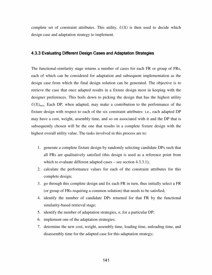
complete set of constraint attributes. This utility, U(X) is then used to decide which

design case and adaptation strategy to implement.

&&&&�#�#��#�#��#�#��#�#�6%� �� "�� "� �� 6%� �� "�� "� �� 6%� �� "�� "� �� 6%� �� "�� "� ��

The functional-similarity stage returns a number of cases for each FR or group of FRs,

each of which can be considered for adaptation and subsequent implementation as the

design case from which the final design solution can be generated. The objective is to

retrieve the case that once adapted results in a fixture design most in keeping with the

designer preferences. This boils down to picking the design that has the highest utility

U(X)max. Each DP, when adapted, may make a contribution to the performance of the

fixture design with respect to each of the six constraint attributes: i.e., each adapted DP

may have a cost, weight, assembly time, and so on associated with it and the DP that is

subsequently chosen will be the one that results in a complete fixture design with the

highest overall utility value. The tasks involved in this process are to:

1. generate a complete fixture design by randomly selecting candidate DPs such that

all FRs are qualitatively satisfied (this design is used as a reference point from

which to evaluate different adapted cases – see section 4.3.3.1);

2. calculate the performance values for each of the constraint attributes for this

complete design;

3. go through this complete design and fix each FR in turn, thus initially select a FR

(or group of FRs requiring a common solution) that needs to be satisfied;

4. identify the number of candidate DPs returned for that FR by the functional

similarity-based retrieval stage;

5. identify the number of adaptation strategies, n, for a particular DP;

6. implement one of the adaptation strategies;

7. determine the new cost, weight, assembly time, loading time, unloading time, and

disassembly time for the adapted case for this adaptation strategy;

�&!�

8. incorporate these values into the overall cost, weight, etc., of the complete fixture

design;

9. determine the overall utility of the new complete fixture design;

10. repeat steps 5 to 7 for each adaptation strategy;

11. compare the overall utility values for each adaptation strategy and select the

strategy with the highest utility value Umax(DPcase_id/n_max) where n_max denotes

the best adaptation strategy and case_id represents the DP identification;

12. repeat steps 4 to 9 for each candidate case for each FR or group of FRs;

13. compare the values of Umax(DPcase_id/n_max) for each DP and select the

DP/adaptation strategy combination that returns the highest utility as the final

design solution for that FR or group of FRs;

14. repeat steps 3 to 13 until all FRs are satisfied;

15. output the final design solution to the user.

The outputs of this retrieval stage are the completed unit and element schemas for each of

the units that return the highest utility value for a particular FR. The schemas contain the

details of the adapted cases.

&�#&�#&�#&�#�#�#�#�#��4 � � � �� "��4 � � � �� "��4 � � � �� "��4 � � � �� "� ��

The first stage of the adapatability-based retrieval process is to generate a complete

fixture design that qualitatively satisfies the FRs. This complete fixture design provides a

common reference point with which to compare all design cases and their adaptation

strategies. An important point to note about this design is that is highly unlikely to satisfy

the design requirement quantitatively (e.g., it will consist of the right type and number of

units but the individual performance values for each of those units, such as clamping

stiffness, will not be satisfactory), and the procedure adopted is to go through each FR in

turn and implement adaptation strategies for each candidate DP. Once the DP has been

fixed, the analysis can proceed to determining how well this repaired design satisfies the

design preferences.

�&#�

The output of the vetting stage is a list of possible DP solutions for each FR or group of

FRs, as illustrated in Figure 72. The first step is therefore to obtain a complete fixture

design solution by selecting a group of these DPs such that for each FR a DP exists in the

fixture design that attempts to satisfy it. At this stage the DP does not have to

quantitatively satisfy the FR. The simplest way to do this is simply to select the DPs that

were returned first during the vetting stage (highlighted in Figure 72).

FR Possible DP solutions FR2.1.1.1 Provide clamping force of 50 lb against locator P1

VC0132C1 VC0132C2 VC021C3 VC022C1

FR2.1.1.2 Provide clamping force of 50 lb against locator T1

HC022C1 HC022C2 HC022C3 HC021C1

FR2.1.1.3 Provide clamping force of 50 lb against locator S1

HC022C1 HC022C2 HC022C3 HC021C1

Figure 72: A sample list of FRs and possible DP solutions

In case library 2, the details for each of these cases will be held in the standard case

schema. Part of the information held in this schema (Figure 73) contains the functionality

of the DP as well as its individual performance with respect to the global constraint

attributes. Thus the overall fixture design attribute performance levels can be calculated

by summing up the contributions from each individual unit used in the design. For

example cost is equal to:

costoverall = costVC0132C1 + costHC022C1 + costHC022C1 +…………….

�&&�

Figure 73: Part of the schema for a vertical clamp

In this way the cost, assembly time, etc., are calculated for the complete design. When

each DP is subsequently adapted and evaluated, then the attribute performance values

used for the initial design can simply be removed and replaced with the new values for

the adapted DP and the overall utility of the design calculated.

&�#�#&�#�#&�#�#&�#�#�!�� "� �� "� �� !�� "� �� "� �� !�� "� �� "� �� !�� "� �� "� �� ,�� ,�� ,�� , ++++� � �� ''''� �� %� �� %� �� %� �� %� ��

During adaptation, it is necessary to understand the relationships that exist between the

FRs, DPs, and adaptation strategies. In terms of implementing an adaptation strategy, it is

important to understand what parameters of a DP are affected by its implementation,

what limitations exist on using a particular strategy (e.g., where it can be used), and what

the effect upon the DP’s ability to satisfy the design preferences is. To support the

adaptation process, the CAFixD method relies on domain knowledge that it applies for

specific FRs. This knowledge includes both the adaptation strategies themselves as well

as knowledge regarding the FRs and DPs to which they are applicable. Domain

knowledge also determines the effect that a particular adaptation strategy will have upon

an individual DP’s contribution to the performance values for each of the constraint

attributes. Utility analysis is used to determine whether this is a beneficial or detrimental

effect. A convenient representation of the adaptability-based retrieval process is a

Class type Unit ID Stiffness FR performance Clamping force FR performance Acting height Chip shedding ability Unit cost Unit weight Loading time associated with unit Unit assembly time Unloading time associated with unit

�&*�

structure termed the “adaptation mapping layout“, an example of which is presented in

Figure 74.

Figure 74: The adaptation mapping layout

FR2.7

DP2.7a

PV2.7.2a

PV2.7.3a

PV2.7.1a

RelDP2.7.1a RelFR2.7.1a

RelDP2.7.2a RelDP2.7.3a

C12

C13

C10

C11

C8 C9

C1

C2

DP2.7b RelFR2.7.1b Link from PVs to this DP

Parameters affected by implementation of this PV modification

Key: Input/output;

Local constraint limit affecting PV; PV affecting global constraint attributes; PV affecting other parameters

�&9�

Specifically this structure:

• outlines all candidate solutions (DPs) from which a design can be generated;

• shows how all of these candidate DPs can be adapted;

• provides a measure of how well a solution created from a particular DP and

adaptation strategy combination satisfy the design preferences;

• shows the relationships between DPs and the functions they perform.

For each FR (e.g., FR2.7 in Figure 74), there may be any number of possible DPs (DP2.7a,

DP2.7b). The relationships between the FRs and DPs (RelFR) are qualitative and extend to

ensuring that the DP can offer the type of FR that is required. A standard FR may be to

provide a vertical clamping stiffness of 200E6 lb/in and the corresponding DP would be a

clamping unit able to provide a vertical stiffness. If the vertical stiffness provided by the

DP does not match the required value, then suitable adaptation strategies need to be

identified and subsequently evaluated. These adaptation strategies modify a particular PV

of a DP. PVs are general concepts such as DP thickness or material type. An adaptation

strategy will change a PV using a statement such as “Apply an increase of 0.5 inches to

the thickness PV for DP2.7a”. The task of actually implementating such a change to the

elements within a DP can be fairly complex. Many elements within a DP may need to be

modified to accommodate this PV change and adaptation strategies contain the details of

the elements affected.

The nature of the RelDP relationships tends to be more complex than those that exist

between the FRs and DPs and extends to understanding how the structure of a DP

achieves its function. Essentially the relationships represent the behaviour of a DP. This

understanding of the behaviour of DPs is used to determine the structural modifications

necessary to achieve the desired FR. The role of the adaptation strategy is therefore to

determine the PV change, implement it, and then test the revised DP to ensure that it

works

�&:�

Once an adaptation strategy has been successfully implemented the effect of the DP’s

contribution to the performance of the complete fixture design with respect to the design

preferences can begin. The relationships between the parameters of the design and the

global constraint attributes are known. That is, for each unit, relationships exist within the

domain knowledge base that can be used to calculate an individual unit’s cost, weight,

etc. These calculated values can subsequently be incorporated into the constraint attribute

performance values for the complete fixture design, allowing the overall utility of a

particular DP and adaptation strategy combination to be obtained. This utility can then be

compared with those of other DP/adaptation strategy combinations to ascertain the most

preferred option: i.e., the DP/adaptation strategy with the highest utility.

When implementing an adaptation strategy, certain limitations may exist on what can be

done and these are represented by the local constraints associated with the PVs. Simple

examples are a limit on the number of materials that exist within the domain knowledge

base, or a limit on the maximum dimensional modification of an element. For example,

Figure 75 illustrates that the thickness of the horizontal element of the locating unit

cannot be greater than 2l otherwise the element will collide with fixture base.

This form of collision detection is the main type of interference checking that the

CAFixD method supports and it plays a particularly prominent role when evaluating how

a DP should be changed when implementing an adaptation strategy. Specific adaptation

strategies and issues arising from their invocation are discussed in section 4.3.3.2.1. The

evaluation of different DP/adaptation strategy combinations is discussed in section

4.3.3.2.2.

�&<�

Figure 75: Local constraint limiting a dimensional change

&�#�#&�#�#&�#�#&�#�#�!�� !�� !�� !��

Possible adaptation strategies are identified within the domain knowledge base by using

simple rules. It is essentially a two stage process in which initially the type of FR is

evaluated. Then the type of DP determines the possible adaptation strategies. Figure 76

represents a pseudo-code implementation of the process.

Upon initially determining the type of FR the search for the appropriate adaptation

strategy is then driven by the type of DP being considered as a solution for that FR. For

vertical clamps used to satisfy a clamping stiffness, three possible adaptation strategies

exist. One alters the thickness of the components of the DP, the second their width, and

the third the material properties of the unit components. Strategies have a modification

module, a testing module, and a control module. The modification module makes the

physical changes to a DP, which is then subjected to testing by the testing module. The

control module evaluates the testing results to determine if a satisfactory stiffness has

been attained. If not then the control module asks the modification module to modify the

DP again, and it is the job of the control module to inform the modification module of the

magnitude of the design change. The modification module manages the implementation

of this change to the individual elements. This process is repeated until either a

satisfactory solution has been achieved or the control module deems that the adaptation

l

Element thickness cannot exceed 2l

Fixture base

Locating unit

�&=�

strategy is unable to produce a satisfactory solution. If the adaptation is successful then

the modified design is subjected to the evaluation process presented in section 4.3.3.2.2.

If the adaptation strategy is unable to produce a working solution then the retrieval

process moves on to consider the next adaptation strategy for that DP.

If (FR is “vertical_stiffness”) then

If (DP is “strap_clamp”) then

If (DP is “strap_clamp_first_order”) then

Adaptation strategy 1: strap_thickness_adapt( )

Modification module: alter_ thickness( )

Test module: strap_clamp_first_order_disp_func( )

Control module: dimension_control( )

Adaptation strategy 2: strap_width_adapt( )

Modification module: alter_ width( )


Control module: dimension_control( )

Adaptation strategy 3: strap_material_adapt( )

Modification module: alter_ material( )


Control module: material_control( )

If (DP is “strap_clamp_third _order”) then

Adaptation strategy 1:……….…………………………….

If (DP is “toggle_clamp”) then……………………….

If (FR is “vertical_clamping_force”) then If (DP is “strap_clamp”) then

If (DP is “strap_clamp_first_order”) then

If (Force_actuation is “thread”) then

Adaptation strategy: strap_torque( ) Modification module: torque_calc_first_order( )

Test module: torque_calc_first_order( )

Control module: torque_control( )

If ( DP is “strap_clamp_second_order”) then…………………. If (DP is “toggle_clamp”) then………………..

If (FR is “horizontal_stiffness”) then……………………

Figure 76: Pseudo code representation of selecting adaptation strategies

�*> �

Specific issues arise within the modification and control modules. During modification

the interactions that can occur when modifying components within a fixture unit must be

carefully managed. Difficulties within the control module relate to identifying when a

strategy is likely to fail and how to generate an appropriate modification request for the

modification module. Section 4.3.3.2.1.1 describes the modification modules in greater

detail, section 4.3.3.2.1.2 the testing modules, and section 4.3.3.2.1.3 the control

modules.

&�#�#&�#�#&�#�#&�#�#�!��$� � �� $�!��$� � �� $�!��$� � �� $�!��$� � �� $� � � ��

The modification module implements the design change suggested by the control module.

For example if the control module suggests a dimension change of 0.3 inches to the

alter_thickness( ) modification module, then it is the responsibility of the modification

module to determine how the components within a DP must be changed to accommodate

this amendment. During the implementation of an adaptation strategy an important point

to note is the complex interactions that can arise when modifying a design case. To

illustrate some of these difficulties a third order vertical strap clamp, as presented in

Figure 77, will be considered. Changing the material of a unit poses no significant

difficulty, thus discussion will be limited to complications that arise from implementing

the modification modules alter_thickness( ) and alter_width( ), which alter a unit’s

thickness and width respectively. Figure 78 and Figure 79 illustrate the directions in

which thickness and width modifications are made.

�*��

Figure 77: A third order vertical strap clamp and its element skeleton

Figure 78: Thickness changes on a third order vertical strap clamp

elem1

Work limb

Fulcrum limb

Contact limb

elem2 front back

�*!�

Figure 79: Width changes on a third order vertical strap clamp

Within case library 2, each unit is broken down into a number of manageable elements

(for example E1, E2,…..E10 from Figure 77) to facilitate the stiffness analysis detailed in

section 4.3.3.2.1.2. For each element the relevant details are stored in a standard element

schema that is attached to the main unit schema. The unit and element schemas are

recalled for convenience in Table 11 and Table 12. The greyed out entries relate to the

performance of the unit as a whole and have been discussed previously in section 4.2.4.

The areas of interest with regard to adaptation concern the description of the individual

limbs and elements from which the unit is comprised.

The following information is provided about the limbs in the clamping unit schema.

• “Force actuation” – describes the manner by which the clamping force is

produced. This is used to for calculating the loading and unloading time.

• “Total number of elements” – this the total number of elements the unit consists

of and is used to control the number of times the testing module executes.

• “Number of fulcrum/work/beamE1/beamE2 elements” – this lists the number of

elements that exist within each of the limbs of the unit. This information is used

when changing the length and position of elements within each limb.

• The “(Work) L2 element”, “(Fulcrum) L1 element”, and “C beam element”

entries list the elements from the beam that contact the work, fulcrum, and contact

limbs respectively. This information is used to manage interactions that occur

when modifying the width or thickness of the unit.

�*#�

Clamping unit attribute Description Class type Class type within case library 2

Unit ID Identifying name for unit Stiffness FR performance Unit stiffness

Clamping force FR performance Unit clamping force Acting height Contact point with workpiece is 3 inches from

the base of the unit Chip shedding ability Does the unit have a chip shedding ability?

Unit cost Cost of unit ($)

Unit weight Weight of unit (lb) Loading time associated with unit Time taken to load workpiece (mins)

Unit assembly time Time taken to assemble the unit (mins) Unloading time associated with unit Time taken to unload workpiece (mins)

Force actuation Means by which the work force (W) is

produced

Total no. of elements Total number of elements within the unit No. of fulcrum elements Number of elements in the fulcrum limb

No. or work elements Number of elements in the work limb No.of length BeamE1 elements Number of elements in beam_elem1 No.of length BeamE2 elements Number of elements in beam_elem2

Length of L1 L1dimension (inches) Length of L2 L2dimension (inches)

(Work) L2 beam element Beam element to which work limb connects (Fulcrum) L1 beam element Beam element to which fulcrum limb connects

C beam element Beam element to which contact limb connects Work limb max thickness Maximum thickness in the work limb

Fulcrum limb maximum thickness Maximum thickness in the fulcrum limb Contact limb max thickness Maximum thickness in the contact limb

Work element Work element that contacts strap beam Fulcrum element Fulcrum element that contacts strap beam Contact element Contact element that contacts strap beam

Table 11: A schema for a clamping unit (greyed out entries discussed in section 4.2.4)

• “Length of L1” and “Length of L2” are the lengths of beam elem1 and elem2

respectively. They are subject to possible modification and are subsequently used

during the testing analysis to determine both the forces on the work, fulcrum, and

contact elements, and the displacement of the beam when subjected to the

machining forces.

�*&�

• The “Work element”, “Fulcrum element”, and “Contact element” entries list the

elements from each of these limbs that interface with the strap beam. This

information is used to manage interactions that occur when modifying the width

or thickness of the unit.

• The “Work limb max thickness”, “Fulcrum limb max thickness”, and “Contact

limb max thickness” entries are the maximum thicknesses of the work, fulcrum,

and contact limbs respectively. This information is used to help prevent limbs

from colliding into each other during modification.

Element attribute Comment Element # Element number Limb element No. Position along limb Structure type Cross section type Element type Limb the element is situated in) Dist_from_end Distance element is from the end of the beam segment (inches) Length Element length (inches) Start thickness or radius Element thickness at start of element (inches) End thickness or radius Element thickness at end of element (inches) Start width or radius Element width at start of element (inches) End width or radius Element width at end of element (inches) Material mod Material type Height adjust Is the element subject to a height adjustment if the acting

height of the unit has to change? Slot consideration Is there a slot in the element? Slot width Width of slot (inches) Slot length Length of slot (inches) Type of connection What type of connection connects this element to the next

element No. of connections How many connections there are to the next element Offset distance The position of the connections on the element cross section Conn diameter Diameter of the connections (inches) Mated from The element that this element connects from Mated to The element that this element connects to

Table 12: A schema for an individual clamping element

The following information is provided about the individual elements within each limb.

• “Element number” is an identification assignment ascribed to each element.

�**�

• “Limb element number” describes the position of the element relative to other

elements within a particular limb.

• “Structure type” defines the cross sectional nature of the element (circular or

rectangular). This information is primarily used during the testing phase, but for

the critical elements that interact with the beam it is also used to help manage the

interactions that occur between elements during modifications.

• “Element type” specifies whether the element belongs to the contact, work,

fulcrum, beam elem2, beam elem1, front, or back limbs. This information is used

during stiffness testing, and also during modification of element lengths.

• “Dist_from_end” is the distance of the start of an element from the end of the

limb and is subject to change during modification. This is used for stiffness

testing and for altering the position of elements during modification.

• “Length” is the length of the element and this is subject to change during

modification. It is used during stiffness testing.

• “Start thickness” and “End thickness” are the start and end thicknesses of an

element and are subject to change during modification. Rectangular and circular

cross sections are supported, each of which can vary as illustrated in Figure 80.

For circular cross sections, the start and end thicknesses are the start and end radii

of an element.

• “Start width” and “End width” are the start and end widths of an element and are

subject to change during modification. Rectangular cross sections can vary in a

similar manner to that illustrated in Figure 80. For circular cross sections, this

information is redundant as the start and end radii have already been specified.

• “Slot present”, “Slot width”, and “Slot length” detail any slots that may exist on

the element. These are subject to change during modification, and are used during

the testing phase.

• “Material type” lists the material from which the element is constructed. This is

subject to change if the alter_material( ) modification module is implemented.

• “Type of connection” lists the nature of the connection to the neighbouring

element.

�*9�

• The number of connections, their position (connections are usually positioned

around the central axis of the element) and diameter are also listed. The diameter

and position are subject to change during the modification process.

• The “Mated to” and “Mated from” entries list the elements to which the current

element is connected.

Strap clamps work on the basis of a lever (Figure 81) in which a work force, W, is applied

relative to a fulcrum point which in turn produces a force at the opposite end of the lever,

P. P is the useful force exerted on some external body. The purpose of the stiffness

analysis is to determine the displacement of the unit under machining loads. To perform a

stiffness analysis it is necessary to specify the details of each element in the work,

fulcrum, contact, and beam limbs. A finite element analysis is then performed to calculate

the displacement of the unit in which the displacement of each element is calculated and

then summed to ascertain the unit displacement.

During adaptation the dimensions of these elements may increase or decrease, thus their

length, width, or thickness may change. Also their position within the structure maybe

altered. Length changes may occur in the beam, fulcrum, and work elements. Width and

thickness changes may occur in beam, fulcrum, work, or contact elements. The possible

changes to each element are now described in greater detail.

�*:�

Figure 80: Start and end thicknesses for a) rectangular and b) circular cross sections

Figure 81: The forces in a lever arrangement

&�#�#�!��$� � ��, �� &�#�#�!��$� � ��, �� &�#�#�!��$� � ��, �� &�#�#�!��$� � ��, �� 5�7 � � 5�� 5�7 � � 5�� 5�7 � � 5�� 5�7 � � 5�� 6666��

The following information from the schema is used to support the changes in length of

the fulcrum or work elements:

acting height, h;

number of fulcrum or work elements;

limb element number, s_elem;

distance from end, d;

length, l.

Start thickness

End thickness

Start radius

End radius

a) b)

Applied work force, W

Reaction force at fulcrum, F

Resultant force produced by lever, P, which acts on some external body

�*<�

A standard fulcrum limb will take the form presented in Figure 82. If the acting height of

the fulcrum needs to change for a new design then the values of l and d for each element

will change (Figure 83). The new acting height is obtained from the FR that states the

coordinates for this clamping point (the z coordinate is the relevant value). The new

height is used to calculate the change in required length of each element, delta_l, and the

new positions of each element d’. Thus:

New acting height, h’ = z coordinate of clamping point

delta_l = (h’ – h) / number of fulcrum elements

For element x, the dimension changes are:

lx’ = lx + delta_l

dx’ = dx + (s_elemx - 1) * delta_l

Thus for fulcrum element two (E2) in Figure 82:

l2’ = l2 + delta_l

d2’ = d2 + (2 - 1)* delta_l = d2 + delta_l

Figure 82: A standard fulcrum layout

E1

E2

E3 Length l3, s_elem = 3, distance from end = d3

Length l2, s_elem = 2, distance from end = d2

Length l1, s_elem = 1, distance from end = 0

l3

l2

l1 d2

d3

Acting height, h

�*=�

The procedure is the same for the work limb, the sole exception being that the number of

work elements replaces the number of fulcrum elements. The height of the contact

element is not altered. It remains the same and only the fulcrum and work elements are

modified to obtain the correct height of the unit. The height of these elements is altered to

ensure that the clamp can contact the workpiece, but it is not used to control the stiffness

of the unit although height does affect unit stiffness. The procedure adopted is to fix the

height and then proceed to obtain the required stiffness of the unit. This can be achieved

by altering the thickness, width, or material properties of the unit.

Figure 83: Altering the length of a fulcrum element

When altering the thickness or width of the fulcrum limb, the following information from

the schema is required:

the starting thickness or radius of the element, st_t;

the end thickness or radius of the element, end_t;

the starting width or radius of the element, st_w;

the end width or radius of the element, end_w;

the fulcrum beam element (the element that connects to the strap beam);

the structure type.

E1

E2

E3 l3

l2

l1 d2

d3

Acting height, h

l3’

l2’

l1’ d2’

d3’ Acting height, h’

�9> �

Nominally when implementing the thickness adaptation strategy only the st_t and end_t

values would be changed. However, it may be necessary to alter the width values as well

depending on the structure type of the fulcrum beam element. The structure type of an

element states whether the cross section of an element is rectangular or cylindrical in

nature. If it is cylindrical in nature then it is also necessary to increase the width of the

elements in the fulcrum block. Generally the connecting element will be a bolt that must

fit inside the fulcrum element to which it attaches. Thus increasing the thickness of the

bolt effectively means increasing the radius of the bolt. To accommodate this, the widths

of the remaining fulcrum elements need to be increased, as illustrated in Figure 84.

This change is reflected in all the elements of the fulcrum. Similar considerations apply

when modifying the contact and work elements of a clamping unit. A further issue

regarding modification of these three types of limbs is ensuring that the dimension

changes do not result in the units colliding with each other. This is only relevant when

considering thickness changes which are applied across the central axis of each limb as

illustrated in Figure 85. If the value of the thickness change �t is greater than the

available distance between the work and fulcrum elements g then the units will collide. In

such circumstances the option pursued is to increase the length of the beam elements until

the units no longer collide.

�9��

Figure 84: Modifying fulcrum components

Figure 85: Collisions between fulcrum and work limbs

Width increased by �t

Thickness and radius increased by �t

Overhang of cylindrical component needs to be removed

block element block element

block element

cylindrical element

cylindrical element

Plan views:

Side projections:

Original design Thickness modification

Thickness and width modification

Thickness changes (�t) applied across these axes

Distance between work and fulcrum limbs, g

Collision area

�t > g

�9!�

&�#�#�!��!�$� � ��, �� 1 � � � �6&�#�#�!��!�$� � ��, �� 1 � � � �6&�#�#�!��!�$� � ��, �� 1 � � � �6&�#�#�!��!�$� � ��, �� 1 � � � �6��

The beam itself is split into two main limbs, as illustrated in Figure 86. Beam elem2

represents the portion of the beam existing between the work and the contact limbs, and

beam elem1 the portion existing between the work and fulcrum limbs. When the

occurrence of a collision between two limbs exists, then the relevant beam length is

increased until the limbs do not interfere with each other. In the case of the example

presented in Figure 85, L1 would be increased by at least �t.

In practice straps are one piece components. However for the purposes of stiffness

analysis it is necessary to split this single real component into a number of imaginary

components connected together. Already the beam has been split up into limbs elem1 and

elem2 but further subdivisions are often required to allow the stiffness analysis. Consider

for example the plan view of a normal strap beam, as presented in Figure 87.

Figure 86: Splitting up the strap beam (side projection view)

L2 L1

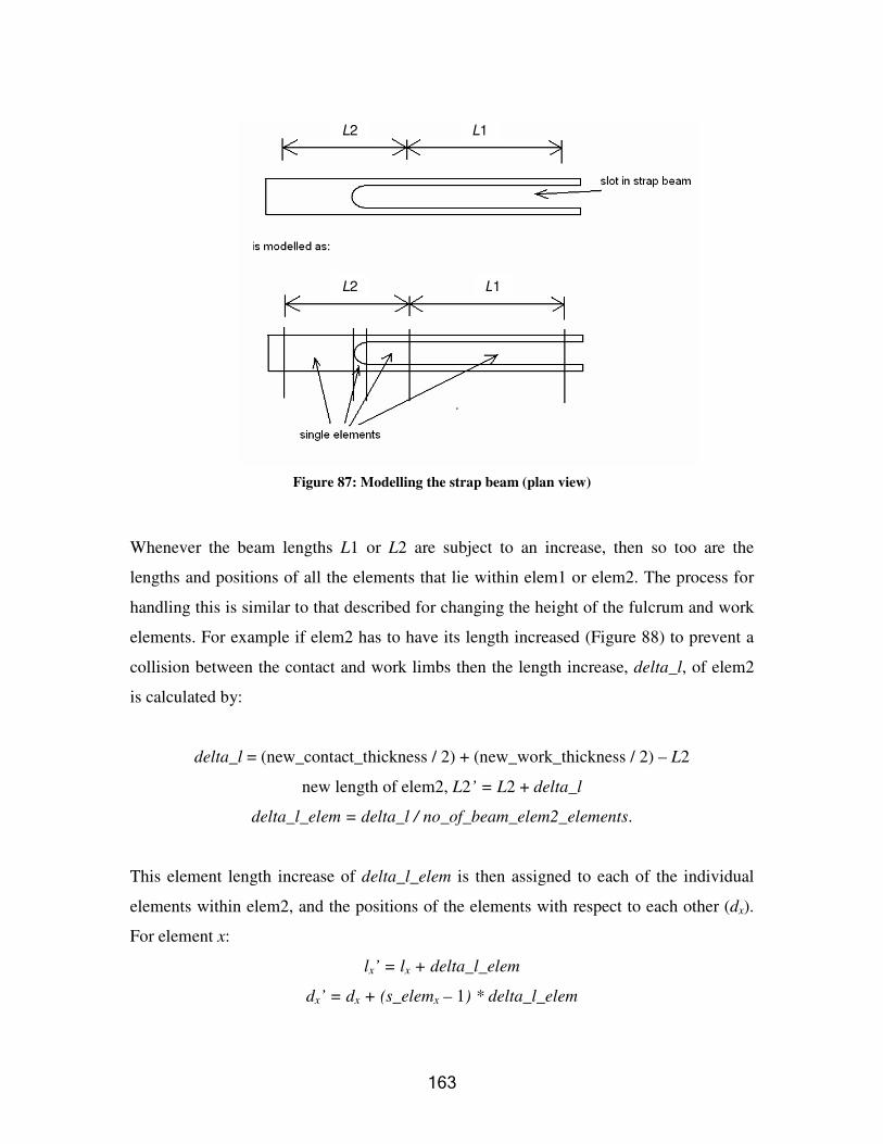
�9#�

Figure 87: Modelling the strap beam (plan view)

Whenever the beam lengths L1 or L2 are subject to an increase, then so too are the

lengths and positions of all the elements that lie within elem1 or elem2. The process for

handling this is similar to that described for changing the height of the fulcrum and work

elements. For example if elem2 has to have its length increased (Figure 88) to prevent a

collision between the contact and work limbs then the length increase, delta_l, of elem2

is calculated by:

delta_l = (new_contact_thickness / 2) + (new_work_thickness / 2) – L2

new length of elem2, L2’ = L2 + delta_l

delta_l_elem = delta_l / no_of_beam_elem2_elements.

This element length increase of delta_l_elem is then assigned to each of the individual

elements within elem2, and the positions of the elements with respect to each other (dx).

For element x:

lx’ = lx + delta_l_elem

dx’ = dx + (s_elemx – 1) * delta_l_elem

L2

L2 L1

L1

�9&�

where s_elemx is the element position number.

Elements may also have their lengths changed as a result of thickness increases to the

work or fulcrum elements that contact the beam. For example if the increase in the work

limb is such that the slot in the workpiece has to be extended then the neighbouring

element to the slot will have to be shortened. At the same time the width of the beam has

to be altered to accommodate the thickness change of the work limb, as illustrated in

Figure 89. If a thickness increase of �t is applied to the work element that interfaces with

the beam, then the beam elements need to be adapted until the slot in the beam, whose

details are listed in the schema, is long enough and wide enough to accept the work

element.

Figure 88: Modifying elements within elem2 (side projection view)

Beam elem2 L2

l1 l2 l3

d3

d2

s_elem = 1 s_elem = 3

s_elem = 2

L2’

l1’ l2’ l3’

d3’

d2’

s_elem = 1 s_elem = 3 s_elem = 2

Increasing L2 results in new dimensions for each element

�9*�

&�#�#�!��#�$� � ��,&�#�#�!��#�$� � ��,&�#�#�!��#�$� � ��,&�#�#�!��#�$� � ��, �� 6�� 6�� 6�� 6��

The connections between elements are also held in the schema. Details include the type

(such as dowel pins, threaded bolt connections, and so on), number, and dimensions of

connections, and the positions of connections. The case schema details which elements

are connected to each other in terms of whom they mate to and whom they mate from.

Elements mate-to other elements away from the workpiece, as illustrated in Figure 90

where element E2 mates to element E3 and element E3 mates from E2. The connection

information held in the schema is for the mates-to connection only. To assist the retrieval

of information for the mating-from connection, the schema contains the identity of the

mates-from element and the required connection information can be retrieved from the

schema entries for this mates-from element.

Figure 89: Modifying elements within the beam due to thickness increases of the work elements

t

t + �t

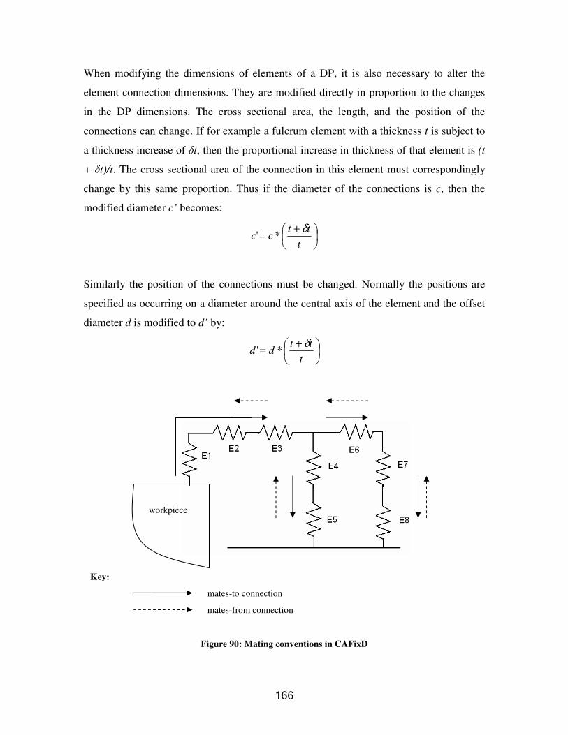
�99�

When modifying the dimensions of elements of a DP, it is also necessary to alter the

element connection dimensions. They are modified directly in proportion to the changes

in the DP dimensions. The cross sectional area, the length, and the position of the

connections can change. If for example a fulcrum element with a thickness t is subject to

a thickness increase of �t, then the proportional increase in thickness of that element is (t

+ �t)/t. The cross sectional area of the connection in this element must correspondingly

change by this same proportion. Thus if the diameter of the connections is c, then the

modified diameter c’ becomes:

�

��

+=t

ttcc δ*'

Similarly the position of the connections must be changed. Normally the positions are

specified as occurring on a diameter around the central axis of the element and the offset diameter d is modified to d’ by:

�

��

+=t

ttdd δ*'

Figure 90: Mating conventions in CAFixD

workpiece

mates-to connection

mates-from connection

Key:

�9:�

Figure 91 illustrates both these changes. The change in length of any connections is similarly dependent on the change in length of the element.

Figure 91: Modifying connection properties on a fulcrum element (cross sectional view)

&�#�#�!��!�� $� � �� "&�#�#�!��!�� $� � �� "&�#�#�!��!�� $� � �� "&�#�#�!��!�� $� � �� "� ��

Once a DP has been altered by a particular modification module, it has to be tested to ascertain how it would behave if used as the design solution. Testing is performed by the

test module of the adaptation strategy. The test performed depends upon the FR the unit is being used to satisfy. If the FR is related to stiffness for example, then a displacement

analysis is carried out on the unit. Continuing with the example of a third order clamping unit, the stiffness FR states that the unit should have a specific stiffness, such that when subjected to a force P during machining, the deflection of the unit d will not be greater

than that allowed by the design tolerance. The purpose of the testing module is to calculate the displacement d (Figure 92).

�

��

+=t

ttcc δ*'

t+�t

c

d

t

�

��

+=t

ttdd δ*'

�9<�

The virtual force method (Hibbler, 1997) is used to carry out the displacement analysis on all locating and clamping units. The principle of virtual force states that the virtual

work done by an external virtual force upon a real displacement system is equal to the virtual work done by internal virtual forces, which are in equilibrium with the external

virtual force, upon the real deformation. Denoting the external virtual work by W and the internal virtual work by VW, the principle of external virtual force can be expressed by:

W = VW (1)

Figure 92: The displacment analysis for a clamping unit

VW represents the strain energy, which is the work done by internal forces. When

applying the principle of virtual force to find a particular deflection at a point, a fictitious unit load is applied at the point of interest and in the direction of the desired deflection.

This unit load is the external virtual force. The external virtual work done by this force P’ is equal to the force magnitude multiplied by the displacement of the real system �. The

internal virtual work is equal to the internal forces (u) caused by the external virtual force P’ multiplied by the internal displacements of the real system �. For simplicity the

magnitude of the external virtual force P is set to 1, thus equation 1 becomes:

� ⋅=∆⋅ dLu1 (2)

P’ = 1 lb = external virtual unit load acting in direction of �;

u = internal virtual load acting on the element (lb);

�9=�

� = external displacement caused by real loads (inches); dL = internal displacement of the element in the direction of u, caused by the real loads

(inches).

The right hand side of equation 2 represents the strain energy of the system. The equations for internal virtual work for a single element as a result of axial and shear force

loads, as well as bending moments, are presented in Table 13, where:

E = Young’s modulus of elasticity of the element material (lb/in); A = cross sectional area of an element (in2);

n = internal virtual axial load caused by the external virtual load (lb); N = internal real axial load acting on an element caused by the real external load (lb);

V = real internal shear load caused by the real external load (lb); v = internal virtual shear caused by the external virtual load (lb);

G = shear modulus of elasticity of the element material (lb/in); M = real internal moment caused by the real external loads (lb.in);

m = virtual internal moment caused by the virtual external loads (lb.in); I = moment of inertia (in4);

L = length of element (in). fs = form factor (a dimensionless number that is unique for a specific cross sectional

area shape).

Deformation caused by Strain energy Internal virtual work

Axial load, N dxEA

NL

�0

2

2 dx

EAnNL

�0 2

Shear load, V �L

s dxGAVf

0

2

2 dx

GAvVfL

o

s�

Bending moment, M dxEI

ML

�0

2

2 �

L

dxEI

mM

0

Table 13: Internal virtual work equations for shear, axial, and bending moment loads (Hibbeler,

1997)

�:> �

The equations for internal virtual work can be incorporated into equation 2 to yield:

� �� ++=∆⋅L L

sL

GAvVf

EImMdx

AEnN

0 00

1 (3)

This equation allows the displacement of the real system � to be calculated. For a third order clamping unit the analysis makes the following assumptions:

1. the strap beam elements are subjected to bending moments and shear forces as a

result of the external force P; 2. bending moments arising at joints between the work, fulcrum, beam, and contact

limbs are neglected.

Thus the clamp is modelled as presented in Figure 93. The contact and fulcrum limbs are in compression with the work limb in tension. The displacement d is a function of the combined displacements dbeam, dcontact, dwork, and dfulcrum, which are the displacements of

the beam, contact, work, and fulcrum limbs respectively:

d = dbeam + dcontact+ dwork + dfulcrum (4)

Thus the solution for d boils down to applying equation 3 to each of the elements in the contact, work, fulcrum, and beam elements to determine their individual displacements

which are then summed using equation 4. The procedure is to:

• create the real and virtual force systems;

• calculate the forces Fw and Ff for the real system;

• apply the virtual unit load and determine the internal virtual forces fw and ff ;

• apply equation 3 to determine the displacement of each element;

• apply equation 4 to determine the displacement d.

�:��

Figure 93 has already presented the real force systems, and the virtual force system for the beam is illustrated in Figure 94. The virtual unit load is placed at the

workpiece/clamping unit interface (fc = 1 lb). The stiffness of the unit must act against the workpiece pushing up against the unit as a result of the machining forces, thus the

displacement d (Figure 92) points in the direction shown as this is the expected direction of movement.

Figure 93: Boundary conditions for the unit stiffness analysis

dbeam

dcontact

dwork

dfulcrum

Fw

Fw

Fw Fc

Fc

Fc

Ff

Ff

Ff

L2 L1

�:!�

Figure 94: The virtual force system

The equations of equilibrium are applied to the strap beam to obtain solutions for the

force. Initially this is done for the real force system.

Figure 95: Obtaining the internal forces for the real system

L2 L1

Fc Ff

Fw Positive sign conventions: Forces: Moments:

fw

fw

fw

fc

fc

fc

ff

ff

ff

L2 L1

�:#�

Equilibrium conditions (positive sign conventions as denoted in Figure 95):

1. � (Moments about Fw) = 0 (Fc * L2) – (Ff * L1) = 0

Ff = Fc*L2 / L1 (5) 2. � (Forces acting in vertical direction) = 0

Fc + Ff – Fw = 0

Fw = Fc + Ff (6)

Fc is the known force (it is calculated when generating the second FR set, FR2, earlier on

in the design process) thus the forces Ff and Fw can be calculated from equations 5 and 6. The process is then repeated for the virtual force system:

Equilibrium conditions:

1. � (Moments about fw) = 0

(fc * L2) – (ff * L1) = 0

ff = fc*L2 / L1

2. � (Forces acting in vertical direction) = 0 fc + ff – fw = 0

fw = fc + ff

The displacement for each element in the DP can now be calculated. To perform the integration required in equation 3, the beam must be split into segments across which

there is continuity of loading. To calculate dbeam, the beam is split into two segments elem1 and elem2.

�:&�

Figure 96: Splitting up the beam

Each of these segments can contain any number of elements. Recalling Figure 92 elem2

has two elements in it whilst elem1 has one. For each element within a segment, the internal forces and moments caused by the external forces need to be calculated. Again

these are calculated using the equilibrium equations for both the real and virtual system of forces. In each case solutions are the internal real or virtual shear forces (V and v

respectively) and the internal real or virtual moments (M and m respectively). Figure 97 presents the solutions for any element i in elem2, and Figure 98 contains the same for any

element j within elem1.

Figure 97: Equilibrium solutions for elem2

x2 x1

Fc

Fw

Ff L2 L1

Mi

Vi Fc

Applying equilibrium yields: Vi = Fc Mi = Vi * x2

x2

mi

vi fc = 1

Applying equilibrium yields: vi = fc = 1 lb mi = vi * x2

x2

Real force system: Virtual force system:

�:*�

Figure 98: Equilibrium solutions for elem1

Now equation 3 can be applied, but the beam is not subjected to an axial loading thus the displacement equation simplifies to:

where:

end_i and end_j are the end positions of the element i or j along axis x2 or x1 respectively; start_i and start_j are the start positions of the element i or j along axis x2 or x1

respectively; Li and Lj are the lengths of the element i or j respectively;

n and p are the number of elements in elem1 and elem2 respectively.

Mj

Vj

Ff

Applying equilibrium yields: Vj = -Ff

Mj = -Vj * x1

x1

Real force system: Virtual force system:

mj

vj

ff

x1

Applying equilibrium yields: vj = -ff

mj = -vj * x1

� � � � ��= = = =

+++=n

i

p

j

iend

istart

n

i

p

j jj

jjjs

ii

iiis

jj

jjiend

istart ii

iibeam AG

LVvfAG

LVvfdxIE

Mmdx

IEMmd

1 1

_

_ 1 112

_

_

.1

Bending component of displacement Shear component of displacement

�:9�

Equation 3 can now be applied to the remaining limbs allowing their respective displacements to be determined. Thus for the fulcrum, work, and contact limbs

containing a, b, and c elements respectively then:

�=

=c

i ii

icccontact EA

LFfd1

*1

�=

=b

i ii

iwwwork EA

LFfd1

*1

�=

=a

i ii

ifffulcrum EA

LFfd

1*1

Figure 99: Calculating dwork for element i

&�#�#&�#�#&�#�#&�#�#�!��#�� !��#�� !��#�� !��#�� ,�� ,�� ,�� , ��

The modification module makes changes to a design which is subsequently tested by the testing module. The control module then evaluates the design using the testing results and

decides what should happen next. Specifically, the control module for a stiffness adaptation strategy will make one of three decisions:

Li

Fw

delem

ii

iwwelem EA

LFfd =

Base or connecting element

element

�::�

1. If the modified DP satisfies the functional requirement for which it is in intended, then the DP is passed to the DP/adaptation strategy evaluator (detailed in section

4.3.3.2.2). 2. If the modified DP does not satisfy the functional requirement but the control

module still feels that a working solution can be achieved, then the DP is returned to the modification module with suggestions for an appropriate alteration.

3. If the modified DP does not satisfy the functional requirement and the control module feels that a working solution cannot be achieved with this adaptation

strategy, then the adaptation strategy is abandoned and the design process moves on to consider the next possible adaptation strategy.

Two control modules will be discussed – the dimension_control( ) and the

material_control( ) modules. The dimension_control( ) module controls the execution of the alter-thickness( ) and alter_width( ) modification modules, while material_control( )

drives the alter_material( ) module.

Figure 100 presents the execution path of a dimension_control( ) module. One of the first tasks the module performs is to compare the displacement of the DP (calc_disp is

obtained from implementing a call to the testing module) to that required in the FR (des_disp). A satisfactory design is obtained when the difference between the calculated

and design displacement is less than a pre-specified computational accuracy (des_accuracy). If the calculated displacement is greater than the design displacement

then the unit needs to have its dimensions increased to afford an enlargement in unit stiffness. An initial basic dimension change (dim_change) is applied to the DP and tested,

and the control module modifies the value of dim_change until calc_disp and des_disp are in agreement.

�:<�

Figure 100: Flow diagram of dimension_control( ) module

Call test_module( ) to calculate calc_disp

Is |calc_disp – des_disp| > des_accuracy?

No

Move to DP/adaptation strategy evaluation module

Yes

Has calc_disp – des_disp polarity reversed?

Yes

step = -(step/10)

dim_change = dim_change + step

Set intial values for dim_change and step

Call modification_module( )

Has adaptation strategy failure criteria been met?

No

Yes

No

Call test_module( ) to calculate calc_disp Abandon this

adaptation strategy and move on to next one or if none exists then move to next FR

�:=�

dim_change is altered by a value step each time the control loop executes. The step value is gradually refined each time there is a crossover in the polarity of (calc_disp –

des_disp). Consider that the loop is in operation and a changeover has occurred on the 10th execution of the loop, as illustrated in Table 14. At the beginning of the ninth loop,

the dimension change is 1.8 with a step of 0.1. The testing module has returned a value for calc_disp which is greater than des_disp. Thus the dimension has to be increased

again to increase the stiffness so the new value for dim_change is:

dim_change’ = dim_change + step = 1.8 + 0.1 = 1.9

At the end of ninth loop the dimension change is 1.9 inches, with a step increment of 0.1 inches. This dimension change is passed to the modification module, implemented, and

subsequently tested. During loop ten, the control module evaluates the results of this testing and deduces that the modified unit is now stronger than necessary because

calc_disp is less than des_disp. (calc_disp – des_disp) has gone from having a positive to a negative polarity and the solution for the dimension change lies somewhere between 1.8

and 1.9. The value of step is refined by dividing it by 10 and reversing its polarity. At the end of loop 10 dim_change has a value of 1.89 and the new value of step is -0.01 inches.

This design is tested and the process repeated until a value of dim_change is ascertained that results in agreement in the values of calc_disp and des_disp within the desired

computational accuracy. When this occurs, the control module sends the DP to the DP/adaptation strategy evaluation module for further analysis in terms of the DP’s

performance with respect to the design preferences.

Loop cycle no. dim_change step Polarity of calc_disp – des_disp 8 1.8 0.1 + 9 1.9 0.1 -

10 1.89 -0.01 - 11 1.88 -0.01 -

Table 14: Refining the dimension change

�<> �

The control module also monitors progress of the solution to determine if any of the criteria for abandoning an adaptation strategy have been met. These criteria define when

an adaptation strategy is likely to fail. Two criteria are used, one of which is related to the polarity reversal of (calc_disp – des_disp). The second concerns the effect design

modifications have on the performance level of the DP.

With regard to monitoring the polarity reversal of (calc_disp – des_disp), failure by this criterion can be identified reasonably early on in the control loop execution. If the loop

continues to execute without a polarity reversal occurring, then the adaptation strategy is aborted. An example of where an adaptation strategy might fail is the

width_modification( ) module for a vertical clamp. Increasing the width dimensions of the elements can result in collision between the work, contact, and fulcrum elements (this

issue was discussed in section 4.3.3.2.1.2) for which the solution is to increase the length of the strap beam until there are no collisions. However, although increasing the

dimensions of the elements increases the unit stiffness, lengthening the beam decreases the stiffness of the strap, particularly with regard to the displacement induced by bending.

The net effect therefore will be a reduction in the effectiveness of the width alteration,

although it may still be a positive effect. The control module however will determine that after a number of attempts at modification without a polarity reversal, the adaptation is

not worth pursuing. If this effect however is more detrimental than the positive effect induced by the width increase, then the solution strategy is doomed to failure and if left to

run, the loop would execute for infinity. To counteract this possibility, the control module applies the second criterion that checks to see if the strategy is resulting in an improved

stiffness. If it finds however that increasing the width is consistently resulting in a decrease in stiffness of the unit, then the strategy is aborted as failed and the next strategy

implemented and evaluated.

The material_control( ) module (Figure 101) is much simpler. The modification module simply cycles through each of the materials that are held in the domain knowledge base,

implementing each one. The testing module calculates the displacement of the DP and the

�<��

control module determines if the behaviour of the DP is acceptable or not. If the FR is satisfied then the control module passes the DP onto the DP/adaptation strategy

evaluation module for further consideration. If the FR is not satisfied then the next material is tried.

Figure 101: The material_control( ) module

&�#�#&�#�#&�#�#&�#�#�!�!�6%� �� "�� "�!�!�6%� �� "�� "�!�!�6%� �� "�� "�!�!�6%� �� "�� ". 8�. 8�. 8�. 8�� , �� , �� , �� , ��

Once an adaptation strategy has been successfully implemented then the DP is further

evaluated by considering how well it contributes to the overall fixture design’s ability to

Call test_module( ) to calculate calc_disp

Is calc_disp < des_disp? Yes

Move to DP/adaptation strategy evaluation module

No

Set material type

Call modification_module( )

No

Yes

Are there any material alternatives left to try?

Abandon this adaptation strategy and move on to next one or if none exists then move on to the next FR

�<!�

satisfy the design preferences recorded by the user in the utility curves. These utility curves express preferences for the global constraint attribute values of the design, to each

of which the DP may or may not make a contribution. A set of functions are invoked to determine the individual contributions that a DP will make.

These functions are essentially heuristic in nature. In particular, functions exist to

determine the cost, weight, and loading, assembly, unloading, and disassembly times of the fixture units. For example the cost of a locating unit is dependent upon the unit

material type, the volume of material used in the unit, the accuracy required of the unit, and the connections used within the unit:

Locating unit cost ($) = f(material type, volume, locating accuracy, connection type,

number of connections)

= volume * material cost per unit volume + cost of connection type * number of

connections + cost of accuracy

This function is applied to each element of the unit and the cost of each element summed to determine the cost for the complete unit. Costs of different materials and connections

are widely accessible in available literature (Callister, 2000). For the purposes of the CAFixD method, accuracy costs are determined from assumed relationships such as that

presented in Figure 102.

The function that calculates the assembly time of a particular unit is dependent upon the number and type of connections between elements. Similar to the cost function, assembly

time is calculated for each individual element and then summed to obtain the time for the entire unit. Different types of connections include:

• Dowel pin connections;

• Threaded bolt connections;

• Snap fit connections;

• Alignment only connections;

�<#�

• Rivet connections;

• Insert connections;

• Nut and bolt threaded connections.

0.0000

0.2000

0.4000

0.6000

0.8000

1.0000

1.2000

0.0000 0.0500 0.1000 0.1500 0.2000 0.2500 0.3000Tolerance (inches)

Cost

($)

Figure 102: An assumed accuracy cost function

Whenever an element is physically assembled into a unit, there are a number of operations that need to be performed. These can include:

• retrieval operations in which an element and possibly tools for assembling the

element need to physically retrieved;

• orientation operations in which elements and/or tools need to be correctly

oriented;

• alignment operations in which elements and/or tools need to be correctly aligned;

• insertion operations in which elements and/or tools are inserted into other

elements/tools;

• screw operations when two elements are joined by screwing them together or

screwing a third element such as a nut to join them together;

• push operations in which elements are joined by some form of interference fit;

�<&�

• rivet operations in which two elements are riveted together.

The CAFixD method has a database of standard times for executing any of the above

operations. Each of the connection types will involve a different number of these operations, and the assembly time associated with a particular type of connection cost is

dependent upon the type and number of these operations. For example a bolt connection will involve the following operations:

• 3 retrieval operations – the element, bolt, and wrench for tightening the bolt must

all be retrieved;

• 3 orientation operations – the element, bolt, and wrench must all be orientated

properly;

• 3 alignment operations – the element must be aligned to its mating element, the

bolt must be aligned to the mating hole in the element, and the wrench must be

aligned with the bolt;

• 2 insertion operations – the bolt must be inserted into the element mating hole and

the wrench must mate with the bolt head;

• 1 screw operation – the bolt must be tightened.

Thus the assembly time for a screw connection, tassembly is:

tassembly = 3 * tretrieval + 3 * torientation + 3 * talignment + 2 * tinsertion + 1 * tscrew

where toperation represents the time recorded in the database for the particular operation

named. Similar approaches are adopted for the remaining functions that determine loading, disassembly, and unloading times.

Once the performance values for each of the constraint attributes have been determined

for a single DP, the DP and these performance values are added to the initial design set up at the start of the adaptability-based retrieval process (after the original DP used for

the current FR in this design and its associated performance values have been removed).

�<*�

These updated attribute performance values for the complete design can then be compared to the design preferences. The utility values for each of the attributes (Ucost,

Uweight, Uassembly, etc.) can be obtained from the utility curves and combined to generate the overall utility U(X) for the complete fixture design containing this DP/adaptation

strategy combination. U(X) is obtained using the following multiplicative:

( )( ) ��

��

�−�

�

��

� += ∏=

111)(1

n

iiii xUKk

KXU

The U(X) values for all possible DP/adaptation strategy that can be used to satisfy a FR or

group of FRs can be computed and the “adaptation mapping layout” representation of the CAFixD retrieval method can be updated as illustrated in Figure 103 by listing the U(X)

values for each DP/adaptation strategy. The combination that returns the highest U(X) is chosen as the final DP solution. In the example presented in Figure 103 PV2.7.1a returns

the highest U(X) value and would be chosen as the final solution.

This adaptation mapping layout can therefore act as a record of design rationale. It outlines the various possible courses of action, and the reasons for choosing one over

another have been recorded in terms of the utility value U(X) associated with each major design decision.

U(X) = overall utility of the complete set of performance objectives X; xi = performance level of each attribute i; X = set of attributes (x1, x2,….,xn); ki = assessed single attribute scaling constant, Ui(xi) = assessed single attribute utility value i = 1,2,….,n attributes; K = overall scaling constant. K is obtained by normalizing U(X) in the standard way:

( )∏ +=+=

n

iiKkK

111

�<9�

Figure 103: Updating the adaptation mapping layout to include U(X)

The CAFixD method requires that no more than six global constraint attributes be considered and the utility analysis can proceed without any special alterations to the

standard execution of the technique. However in a more general design situation there may be a need to consider a higher number of attributes. The literature review noted that

high numbers of attributes resulted in the utility always tending to 1. To counteract this effect, a simple grouping strategy is proposed for discussion. The procedure is:

FR2.7

DP2.7a

PV2.7.2a

PV2.7.3a

PV2.7.1a

RelDP2.7.1a RelFR2.7.1a

RelDP2.7.2a RelDP2.7.3a

C12

C13

C10

C11

C8 C9

C1

C2

Parameters affected by implementation of this adaptation strategy:

Key: Input/output;

Local constraint limit affecting PV;

PV affecting global constraint attributes;

PV affecting other parameters

U(X) = 0.76

U(X) = 0.72 U(X) = 0.56

�<:�

1. define utility curves and scaling constants for each attribute as per the standard procedure outlined in section 4.3.2.1;

2. split the attributes randomly into j groups such that each group has an even number of attributes in it (where each group should have a maximum of six

attributes); 3. For each group calculate the normalizing constant K using the scaling constants

from that group only to obtain a number of K values K1, K2,……Kj; 4. Calculate the utility for each group U1(x1), U2(x2),…………Uj(xj);

5. To each of these groups apply the same scaling constant value kstandard; 6. If more than six groups exist then repeat steps 2 to 5;

7. If less than six groups exist then calculate Kstandard using kstandard and calculate U(X).

Table 15 illustrates two designs that are almost identical with the exception of their

performance with respect to attribute three (design one has a utility of 0.65 whereas design two has a utility of 0.55) return the same overall utility U(X) for the design of

0.99994. If however the grouping approach is adopted as demonstrated in Table 16 and the attributes are split up into four groups of four, then the results become clearer,.

Design one returns a higher U(X) of 0.9727 whereas design two returns a value of 0.9719. This is the expected result since design one has the higher utility for attribute three. The

obvious limitation to the technique is that it is invalid for situations where attributes cannot be gathered into groups that are the same size. Also, it should be noted that

although the utility tends to one, it will rarely get there but the comparison between U(X) values would have to be performed between numbers that are almost identical. The

proposed method merely makes the comparison simpler by virtue of the fact that there is no need to go to significant numbers of decimal places when comparing different U(X)

values.

�<<�

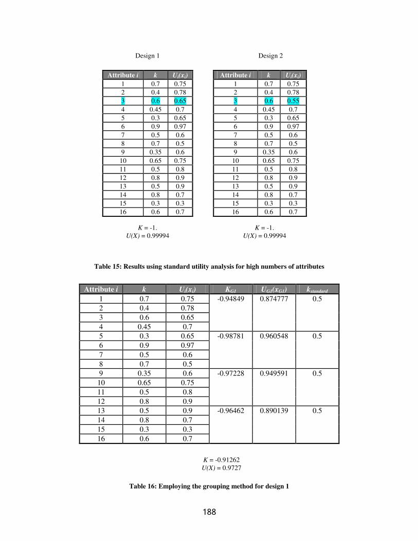
Table 15: Results using standard utility analysis for high numbers of attributes

Attribute i k Ui(xi) KG1 UG1(xG1) kstandard

1 0.7 0.75 2 0.4 0.78 3 0.6 0.65 4 0.45 0.7

-0.94849 0.874777 0.5

5 0.3 0.65 6 0.9 0.97 7 0.5 0.6 8 0.7 0.5

-0.98781 0.960548 0.5

9 0.35 0.6 10 0.65 0.75 11 0.5 0.8 12 0.8 0.9

-0.97228 0.949591 0.5

13 0.5 0.9 14 0.8 0.7 15 0.3 0.3 16 0.6 0.7

-0.96462 0.890139 0.5

Table 16: Employing the grouping method for design 1

Attribute i k Ui(xi) 1 0.7 0.75 2 0.4 0.78 3 0.6 0.65 4 0.45 0.7 5 0.3 0.65 6 0.9 0.97 7 0.5 0.6 8 0.7 0.5 9 0.35 0.6

10 0.65 0.75 11 0.5 0.8 12 0.8 0.9 13 0.5 0.9 14 0.8 0.7 15 0.3 0.3 16 0.6 0.7

K = -1.

U(X) = 0.99994

Attribute i k Ui(xi) 1 0.7 0.75 2 0.4 0.78 3 0.6 0.55 4 0.45 0.7 5 0.3 0.65 6 0.9 0.97 7 0.5 0.6 8 0.7 0.5 9 0.35 0.6

10 0.65 0.75 11 0.5 0.8 12 0.8 0.9 13 0.5 0.9 14 0.8 0.7 15 0.3 0.3 16 0.6 0.7

K = -1.

U(X) = 0.99994

Design 1 Design 2

K = -0.91262 U(X) = 0.9727

�<=�

&�&�&�&�&&&&�'� %�� '� %�� '� %�� '� %��

This chapter has sought to detail the CAFixD method and the manner in which it

navigates towards a solution. Much of the focus within the CAFixD method concerns the indexing and retrieval of design cases. The use of axiomatic design principles assists the

indexing of design cases by function and this is reflected in the hierarchies which exist in the second case library. The retrieval process is strongly linked to a deep understanding

of the manner in which a physical structure behaves: i.e., how the physical characteristics of the structure allow it to perform its functions. Basing the retrieval mechanism upon

structure behaviour adds a certain flexibility to the method in that there are various means by which a design can be repaired. If one strategy fails then another can be tried, and this

ability to implement alternative methods of repairing cases can afford a greater probability of returning a satisfactory solution.

�=> �

�� *�� *�� *�� *��7 � � � � ��7 � � � � ��7 � � � � ��7 � � � � �6666 � � � ��

Chapter 4 detailed the CAFixD method. This chapter presents two examples, the first of which illustrates how a design case is stored in case library 2. The second presents an

example of the operation of the CAFixD method, in which a fixture design is generated for a given workpiece.

****�� 6� �� 6� �� 6� �� 6 � � � ��

Design case 2 consists of a series of types of fixture units, such as the clamping unit

presented in Figure 104a. The unit is a third order vertical clamping unit, where the work force is applied by a threaded bolt upon the strap clamp. It provides a stiffness of 17765

lb/in of and a clamping force of 35lb. The unit itself is composed of 6 components but is described as being composed of 10 elements to aid any stiffness analysis it may be

subject to. The strap beam is the component that has been split into 5 artificial elements, as illustrated in the element representation presented in Figure 104b. The completed

schema for the unit is presented in Table 17 and the completed element schema for element 4 is presented in Table 18. Appendix B presents the full case schema and

drawings for the clamping unit. It is worthwhile noting that the system implementation of the CAFixD methd only supports the units listed in the schema tables.

�=��

Figure 104: A vertical clamping unit

work elements (E7, E8) fulcrum

elements (E9, E10)

contact elements

(E1)

Beam elements (E2, E3, E4, E5, E6)

a) clamping unit b) equivalent element representation

elem2 elem1 Front

fulcrum work

contact

Back

�=!�

Clamping unit attribute Value Comment Class type VC0132 Class type within case library 2

Unit ID VC0132C1 Identifying name for unit Stiffness FR performance 17765 lb/in Unit stiffness

Clamping force FR performance 35 lb Unit clamping force Acting height 3 inches Contact point with workpiece is 3

inches from the base of the unit Chip shedding ability No Does the unit have a chip

shedding ability?

Unit cost $ 1.825566 - Unit weight 1.199557 lb -

Loading time associated with unit 0.583333 mins - Unit assembly time 4.816667 mins -

Unloading time associated with unit 0.45 mins

-

Force actuation TO1A Threaded bolt force actuation

Total no. of elements 10 Total number of elements within

the unit No. of fulcrum elements 2 Number of elements in the

fulcrum limb No. or work elements 2 Number of elements in the work

limb No.of length BeamE1 elements 1 Number of elements in

beam_elem1 No.of length BeamE2 elements 2 Number of elements in

beam_elem2 Length of L1 1.5 inches Length of L2 2 inches

(Work) L2 beam element 4 Beam element to which work limb connects

(Fulcrum) L1 beam element 5 Beam element to which fulcrum limb connects

C beam element 2 Beam element to which contact limb connects

Work limb max thickness 0.8 inches Maximum thickness in the work limb

Fulcrum limb maximum thickness

0.8 inches Maximum thickness in the fulcrum limb

Contact limb max thickness 0.4 inches Maximum thickness in the contact limb

Work element 7 Work element that contacts strap beam

Fulcrum element 9 Fulcrum element that contacts strap beam

Contact element 1 Contact element that contacts strap beam

Table 17: The completed schema for the clamping unit

�=#�

Element attribute Value Comment Element # 4 Element number Limb Element No. 2 Position along limb Structure type Block Cross section Element type beam_elem2 Limb element is situated in Dist from end 1.5 inches Distance element is from the end

of beam_elem2 Length 0.5 inches Element length Start CS b or radius 0.5 inches Element thickness at start of

element End CS b or radius 0.5 inches Element thickness at end of

element Start CS h or radius 0.6 inches Element width at start of element End CS h or radius 0.6 inches Element width at endof element Material mod StSteel304 Material type Height adjust No Is the element subject to a height

adjustment? Slot consideration Yes Is there a slot in the element? Slot width 0.3 inches Width of slot Available slot length 0.5 inches Length of slot Connection to next element None Not a real component so the

connection type is none (connection details are not applicable to this element)

No. of connections 0 Not applicable to this element Offset distance 0 Not applicable to this element Mated from 3 Mates from element 3 Mated to 5 Mates to element 5 Connection diameter 0 Not applicable to this element

Table 18: Completed element schema for element 4

****�!�( � � �� 6�!�( � � �� 6�!�( � � �� 6�!�( � � �� 6 � � � ��

The operation of the CAFixD method will be demonstrated through the use of a worked

example in which a fixture will be developed for the workpiece presented in Figure 105. It is a simple workpiece composed of planar surfaces and two holes. Features to be

machined are surfaces 7, 8, and 9 in addition to holes 18 and 19. The CAD model contains all information related to workpiece’s geometry, as well as information defining features (machined surfaces), their tolerances, and non-machined surfaces. Appendix C

provides the complete geometric information for the workpiece. The machining table (Table 19) contains all the information required to machine the workpiece including for

�=&�

example the machining forces, the type of machine tool used, and the direction of tool movement.

*�*�*�*�!��"� �� $!��"� �� $!��"� �� $!��"� �� $� � � ��

The first stage in the solution process is to analyse the datum information to determine

the locating directions. The datums specified in the tolerances are surfaces 2, 3, and 16. The DMSRG for the workpiece is presented in Figure 106. From the summary of the

datum information detailed in Table 20, there are three candidate locating directions. These are checked to determine if they are all mutually perpendicular to each other and

after confirmation of this the next step is to identify the primary, secondary, and tertiary locating directions. Also as all features use these surfaces as their datums, then there is no

need for an extra setup. Thus only one fixture is sought for this workpiece.

The primary locating direction is normally governed by the type of machining operations to be performed and the machine type. To perform the end milling, drilling, and face

machining of the workpiece features using a vertical mill the workpiece must be positioned such that the normal of the machined features 7, 8, 9, 18, and 19 are coincident

with the spindle axis of the machine tool. Thus the primary locating directions must act in the opposite direction to these normals. The orientation of the normals of each of these

features is held in the CAD workpiece model and are summarised in Table 21.

�=*�

Figure 105: The workpiece and design tolerances

1

2

3

1 (underneath)

2 (underneath)

4 (side surface)

3

5

6 (side surface)

7 8 9

14

13

12 11 (side surface opposing surface 10)

15

10

16

19

18

Machined features are 7, 8, 9, 18, and 19. The tolerances for each feature are:

Feature 8: Feature 9:

Feature 18: Feature 19:

Feature 7:

�=9�

Machine type

Tool accuracy

Along x axis (inches)

Along y axis (inches)

Along z axis

(inches)

Around x axis (rad)

Around y axis (rad)

Around z axis (rad)

Vertical mill 0.00002 0.00002 0.00002 8.75E-5 8.75E-5 8.75E-5

Initial Direction of

tool motion Feature

ID Operation

type Toolpath Tangential

force (lb) Thrust

force (lb) x y z

7 FACE SPIRAL 23 354 0 0 -1 8 ENDMILL BACKFORTH 50 150 0 0 -1 9 ENDMILL BACKFORTH 50 150 0 0 -1

18 DRILL INOUT 50 200 0 -1 0 19 DRILL INOUT 50 200 0 -1 0

Table 19: The machining information

Datum surface Datum orientation Features with this

datum Number of times datum referenced

2 0,1,0 7, 8, 9, 18, 19 5 3 0,0,1 18,19 2

16 1,0,0 18,19 2 Table 20: Tabular format of DMSRG

Figure 106: The DMSRG for the workpiece

�=:�

Feature Feature type Orientation of normal

7 Plane 0,-1,0 8 Plane 0,-1,0 9 Plane 0,-1,0

18 Hole 0,-1,0 19 Hole 0,-1,0

Table 21: Orientation of normals for each machined feature

All features have a normal orientation of (0,-1,0) thus the primary locating direction

should be the opposite of this orientation (0,1,0) and from Table 20 the only datum having this orientation is surface 2. Of the two remaining datum directions in Table 20,

no decision is made concerning which should provide the direction of secondary and tertiary locating should act in. Thus Table 20 can be updated as highlighted in Table 22

by assigning known locating directions.

Datum surface

Datum orientation

Features with this datum

Number of times datum

referenced

Locating direction

2 0,1,0 7, 8, 9, 18, 19 5 Primary 3 0,0,1 18,19 2 Secondary or tertiary

16 1,0,0 18,19 2 Secondary or tertiary

Table 22: Refining the selection of primary, secondary, and tertiary locating directions

The next step is to identify the locating faces and coordinates of locating points. The

objective of this part of the design process is to maximise the area of location provided by the fixture. For each orientation, workpiece surfaces exhibiting this orientation are grouped together and evaluated for possible use as locating surfaces. Consider primary

locating, where two workpiece surfaces (1 and 2) have the correct orientation. Both surfaces are plane surfaces, and thus for primary locating three locating points need to be

used to constrain the required three degrees of freedom. Locating point P1 must constrain linear movement along the y axis, P2 constrain rotation around the x axis, and P3

�=<�

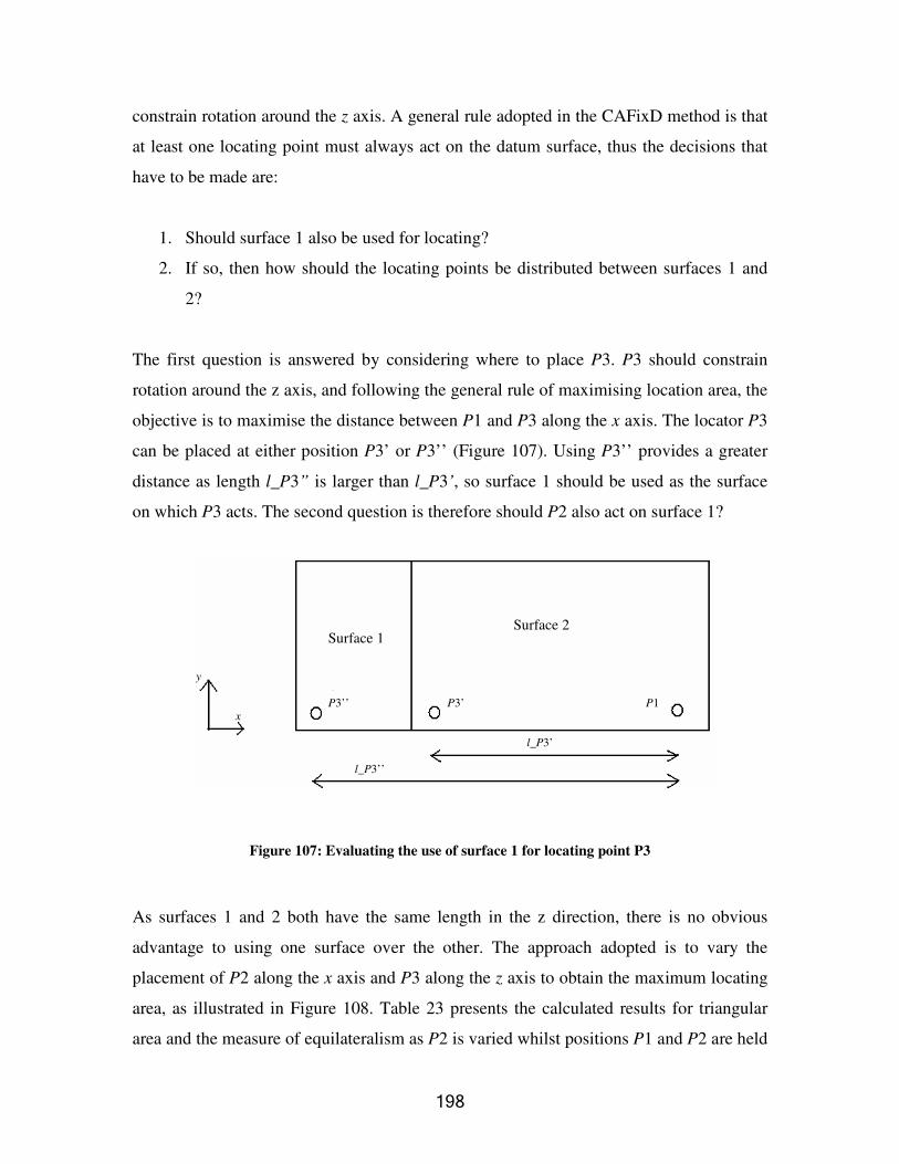
constrain rotation around the z axis. A general rule adopted in the CAFixD method is that at least one locating point must always act on the datum surface, thus the decisions that

have to be made are:

1. Should surface 1 also be used for locating? 2. If so, then how should the locating points be distributed between surfaces 1 and

2?

The first question is answered by considering where to place P3. P3 should constrain rotation around the z axis, and following the general rule of maximising location area, the

objective is to maximise the distance between P1 and P3 along the x axis. The locator P3 can be placed at either position P3’ or P3’’ (Figure 107). Using P3’’ provides a greater

distance as length l_P3” is larger than l_P3’, so surface 1 should be used as the surface on which P3 acts. The second question is therefore should P2 also act on surface 1?

Figure 107: Evaluating the use of surface 1 for locating point P3

As surfaces 1 and 2 both have the same length in the z direction, there is no obvious

advantage to using one surface over the other. The approach adopted is to vary the placement of P2 along the x axis and P3 along the z axis to obtain the maximum locating

area, as illustrated in Figure 108. Table 23 presents the calculated results for triangular area and the measure of equilateralism as P2 is varied whilst positions P1 and P2 are held

l_P3’’

l_P3’

P1 P3’ P3’’

Surface 2 Surface 1

x

y

�==�

constant. The highlighted entry represents the most desirable choice for P2, so P2 is situated on surface 2.

Figure 108: Maximising the locating area

P2 x P2 z Surface P2 exists on

Area Measure of equilateralism

6.75 4.75 2 14.625 0.69457 6.306 4.75 2 14.625 0.718863 5.861 4.75 2 14.625 0.749036 5.417 4.75 2 14.625 0.785248 4.972 4.75 2 14.625 0.827534 4.528 4.75 2 14.625 0.845219 4.083 4.75 2 14.625 0.866349 3.639 4.75 2 14.625 0.893152 3.194 4.75 2 14.625 0.882449 2.75 4.75 2 14.625 0.857751 2.306 4.75 1 14.625 0.838787 1.861 4.75 1 14.625 0.810969 1.417 4.75 1 14.625 0.770956 0.972 4.75 1 14.625 0.73702 0.528 4.75 1 14.625 0.709077

0 4.75 1 14.625 0.683388

Table 23: Determining the optimum position for P2

A similar process is repeated to determine which direction should be used to provide secondary locating. Whichever orientation (and subsequent surfaces with this orientation)

Using different positions of P2

Surface 2 P3 can be moved as well

x

y

Surface 1

P1 P1

P3

!> > �

offers the greatest distance between locators (only two locators are used in secondary locating) is chosen as the secondary locating direction. Using this criterion surface 3

provides secondary locating and surface 16 tertiary. All surfaces used for locating are planar in nature, thus plane locating 3-2-1 variation 3 and its associated skeleton FR set

can be retrieved from case library 1. Thus the setup and fixture planning stages are complete, resulting in the conceptual plan detailed in Figure 109 and Table 24. FRs 1.1.1

and 1.1.2 and their DPs can be updated with these details, as illustrated in Figure 110.

Figure 109: The locating point distribution of conceptual design

Relevant FRs Locator Surface Coordinates

1.1.1.1 & 1.1.2.1 Primary (P1) 2 (6.75,1,0.25) 1.1.1.2 & 1.1.2.2 Tertiary (T1) 16 (0,2.5,2.5) 1.1.1.3 & 1.1.2.3 Secondary (S1) 3 (0.25,2.25,0) 1.1.1.4 & 1.1.2.4 Primary(P2) 2 (3.639,1,4.75) 1.1.1.5 & 1.1.2.5 Secondary (S2) 3 (5.75,2.25,0) 1.1.1.6 & 1.1.2.6 Primary (P3) 1 (0.25,0,0.25)

Table 24: The conceptual design details

P3

P2 (situated on bottom surface)

P1

S2 S1

T1

!> ��

FR1 – Locate workpiece to required accuracy FR1.1 – Locate the workpiece FR1.1.1 – Control six degrees of freedom (6 FRs) FR1.1.1.1 – Control DoF along the y axis FR1.1.1.2 – Control DoF along the x axis FR1.1.1.3 – Control DoF along the z axis FR1.1.1.4 – Control DoF around the x axis FR1.1.1.5 – Control DoF around the y axis FR1.1.1.6 – Control DoF around the z axis FR1.1.2 – Provide contact between locator and workpiece (6FRs) FR1.1.2.1 – Contact workpiece with locator P1 FR1.1.2.2 – Contact workpiece with locator T1 FR1.1.2.3 – Contact workpiece with locator S1 FR1.1.2.4 – Contact workpiece with locator P2 FR1.1.2.5 – Contact workpiece with locator S2 FR1.1.2.6 – Contact workpiece with locator P3

DP1 – Fixture locating arrangement DP 1.1 – 3-2-1 locating principle variation 3 DP 1.1.1 – locator/workpiece interface surface (6DPs) DP1.1.1.1 – Surface 2 DP1.1.1.2 – Surface 16 DP1.1.1.3 – Surface 3 DP1.1.1.4 – Surface 2 DP1.1.1.5 – Surface 3 DP1.1.1.6 – Surface 1 DP 1.1.2 – workpiece/locator interface contact coordinates (6DPs) DP1.1.1.1 – Coordinates (6.75,1, 0.25) DP1.1.1.2 – Coordinates (0,2.5,2.5) DP1.1.1.3 – Coordinates (0.25,2.25,0) DP1.1.1.4 – Coordinates (3.639,1,4.75) DP1.1.1.5 – Coordinates (5.75,2.25,0) DP1.1.1.6 – Coordinates (0.25,0,0.25)

Figure 110: The updated skeleton FR set upon completion of setup and fixture planning

****�!�!�� '��!�!�� '��!�!�� '��!�!�� '��

The solution process now proceeds to performing the sensitivity analysis, with the aim of determining which of the workpiece design tolerances should be used to guide the

tolerance assignment stage. Each locator pair is examined and the effect of any rotation caused by that pair upon the position of the workpiece features calculated and compared to the design tolerance for that feature. This allows the calculation of the sensitivity of the

feature to rotations caused by variations in the locating point pair.

!> !�

Initially locating point pair P1 and P2 will be evaluated. Feature 7 (a rectangular planar surface) has a parallel tolerance of 0.1 inches. The rotation caused by the variation TolP1

and TolP2 will result in vertical shifts at either end of feature 7 causing the start and end

coordinates of the feature to change from S7StartyP1/P2 and S7EndP1/P2 to '7 2/1 PPStartyS

and '7 2/1 PPEndyS respectively. A rotation of 2° is assumed for the rotation.

Figure 111: Analyzing the workpiece tolerances

The new positions can be calculated as follows:

( ) ( ) θθ cos7sin7'7 2/1 xyxyPP CPyEndySCPxEndzSEndyS −+−=

( ) ( ) θθ cos7sin7'7 2/1 xyxyPP CPyStartySCPxStartzSStartyS −+−=

where: S7Startz = original z coordinate of start of feature 7 = 0;

S7Starty = original y coordinate of start of feature 7 = 4.5;

'7 2/1 PPStartyS = new y coordinate of start of feature 7 relative to center point CPzy;

CPzzy = z coordinate of center point between locators P1 and P2 = (0.25 + 4.75)/2 = 2.5; CPyzy = y coordinate of center point between locators P1 and P2 = (1+1)/2 = 1;

CPzy

P2

P1

rotation � TolP1

'7 2/1 PPStartyS

S7EndyP1/P2

z

y

GCS

new surface position caused by rotation

TolP2

S7StartyP1/P2 '7 2/1 PPEndyS

!> #�

� = assumed angle of rotation = 2°; S7Endz = original z coordinate of end of feature 7 = 5;

S7Endy = original y coordinate of end of feature 7 = 4.5;

'7 2/1 PPEndyS = new y coordinate of start of feature 7 relative to center point CPzy.

The resultant shift in the y direction (S7�yP1/P2) is calculated as follows (the answer is

squared and then rooted to give only the magnitude of the shift):

( )22/12/12/1 '7'77 PPPPPP StartySEndySyS −=∆

The sensitivity of this surface tolerance is then determined by:

Sensitivity = S7�yP1/P2/design tolerance

Table 25 presents the results of the sensitivity of feature 7 to variation in locating point pair P1/P2. This entry is compared to other entries for the �y shift caused by locating pair

P1 and P2 in the sensitivity table. As this is the first feature tested the sensitivity table is empty and this would be the first entry, as indicated in Table 26.

Table 25: The sensitivity of feature 7 to variations in locating pair P1 and P2

Feature S7StartyP1/P2’ S7EndyP1/P2’ S7�yP1/P2 Design tolerance

Sensitivity

7 3.910314566 4.084812 0.174497484 0.1 1.7449

!> &�

Table 26: Updating the sensitivity table

The process is then repeated for the remaining tolerance descriptions, resulting in the final sensitivity analysis presented in Table 27. The table contains the feature

identification, the tolerance for that feature, and the calculated sensitivity for the shift in a particular axis direction for each locating point pair. One note of interest is that when

performing the analysis for the P1/P3 locating point pair, the x coordinate of locating point P2 should be used rather than P3. This accounts for the worst case scenario where

constraining the rotational degree of freedom around the x axis is actually performed by locating point P2, as illustrated in Figure 112.

Table 27: The final sensitivity analysis table


rance Sensi-tivity

Feature Tole-rance

Sensit-ivity

Feature Tole-rance

Sensitivi-ty

Max �x/tol shift

0 0 0

Max �y/tol shift

7 TPAR 1.7449 0 0 0

Max �z/tol shift

0 0 0


rance Sensi-tivity

Feature Tole-rance

Sensit-ivity

Feature Tole-rance

Sensitivi-ty

Max �x/tol shift

0 0 0 18 TPER 2.0358 18 TPOS 0.88314

Max �y/tol shift

7 TPAR 1.7449 19 TPOS 1.4821 0 0 0

Max �z/tol shift

18 TPER 2.0358 0 0 0 19 TPOS 0.71321

!> *�

Figure 112: Using the x coordinate of locating point P2 instead of P3 during the sensitivity analysis

Once the sensitivity analysis has been completed, then the allowable tolerance for each locating position can be calculated. This is done for each locating pair and consists of

eight steps.

1. For each locator pair, identify the most sensitive tolerance. 2. Determine the type of tolerance, its value, and the sensitivity.

3. Recalculate the shift caused in the relevant direction by the locator pair. 4. Determine the final tolerance allowed for that feature in the current direction.

5. Estimate the allowed angle of rotation using the sensitivity value. 6. Calculate the shift caused by this estimated angle.

7. Refine the estimated value of the allowed angle of rotation. 8. Calculate the allowed tolerances for the locator pair.

Consider the P1/P2 locating point pair. From the sensitivity analysis results the critical

tolerance is the perpendicular tolerance of hole 18, for which the sensitivity is 2.0358, and the design tolerance is 0.06 inches. The shift in the z direction caused by the assumed rotation of 2° is:

�zP1/P2_Feature18 = Sensitivity * design tolerance = 2.0358 * 0.06 = 0.12214 inches

TolP3

+TolP2 -TolP1

Rotation caused by locating point P2 is greater than that caused by P3

Rotation caused by locating point P3

P1

P2 P3

!> 9�

The perpendicular tolerance on hole 18 dictates that the hole axis must be perpendicular to surface 2 within a range of 0.06 inches, as illustrated in Figure 113. The allowed

tolerance zone for a perpendicular tolerance in a particular direction is assumed to be equal to the length of a square that can fit within the circle created by the TPER tolerance

(Figure 114).

Allowed tolerance = (Design tolerance) * sin 45° = 0.06 * sin 45° = 0.04243 inches

Figure 113: The perpendicular tolerance on hole 18

Figure 114: The allowed design tolerance on hole 18

Design tolerance = 0.06 inches

Allowed location tolerance

45° angle

Perpendicular tolerance = 0.06 inches

Hole axis

a) Side view b) Plan view

Hole

Perpendicular tolerance = 0.06 inches

!> :�

Determining the allowed angle of rotation caused by locating tolerances, �tol, is a two stage process. Initially, an estimate of this angle, �estimate is obtained using the sensitivity

value from the sensitivity table:

�estimate = (allowed tolerance / shift in z direction caused by 2°) * 2°

= (0.042426 / 0.12214) * 2

= 0.69467°

This is only an estimate of the allowed angle of rotation. To check its accuracy, the angle has to be fed back into the equations used to determine the shift in position of a surface

caused by a rotation during the sensitivity analysis:

( ) ( ) θθ sin18cos1818'18 2/1 zyzyPP CPyStartySCPzzStartSStartzS −−−=

( ) ( ) θθ sin18cos1818'18 2/1 zyzyPP CPyEndySCPzzEndSEndzS −−−=

where:

S18Startz = original z coordinate of start of hole 18 = 2.5; S18Starty = original y coordinate of start of hole 18 = 4.5;

'18 2/1 PPStartzS = new z coordinate of start of hole 18 relative to center point CP;

CPzzy = z coordinate of center point between locators P1 and P2 = (0.25 + 4.75)/2 = 2.5;

CPyzy = y coordinate of center point between locators P1 and P2 = (1+1)/2 = 1; � = �estimate = 0.0521080;

S18Endz = original z coordinate of end of hole 18 = 2.5; S18Endy = original y coordinate of end of hole 18 = 1;

'18 2/1 PPEndzS = new z coordinate of end of hole 18 relative to center point CP.

The shift of interest is the resultant shift in the z (S18�zP1/P2) direction is therefore:

( )22/12/12/1 '18'1818 PPPPPP EndzSStartzSzS −=∆

Putting in the numbers gives S18�zP1/P2 = 0.042434 inches.

!> <�

This value needs to be compared to the allowed design tolerance determined earlier on (0.042426 inches), thus the similarity measure is obtained by:

Similarity = S18�zP1/P2 / Allowed design tolerance

= 0.042434 / 0.042426 = 1.000189.

Thus, �estimate is a little large (Similarity should equal 1.0000) and needs to be reduced.

This is done by subtracting a standard increment from �estimate until the similarity condition is satisfied. When �estimate = 0.69454674°, the similarity condition is satisfied

(note this is less than the original estimate of 0.69467°). The allowed angle of rotation �tol caused by the location tolerance is:

�tol = 0.69454674° – �m/c_rot

where �m/c_rot is the accuracy of the machine tool around a particular axis and for the

P1/P2 locators the axis of relevance is the x axis. Recalling the machining data detailed in Table 19, �tol becomes 0.68954674°.

The next stage is to use �tol to determine the allowed tolerances at the locating positions

P1 and P2 (TolP1 and TolP2).

Figure 115: Determining TolP1 and TolP2

P1

P2 z

y GCS rotation �tol

CPzy

TolP1 �zCP-P2

�yCP-P2 rotation �loc

TolP2

!> =�

�tol = angle of rotation caused by location tolerance = 0.68954674°

�loc = angle of rotation caused by different y coordinates of locating points = 0°

� = overall angle of rotation = �loc + �tol = 0.68954674°

TolP2 = TolP1 = allowed tolerance for each locator �zCP-P2 = z coordinate P2 – z coordinate CP

= 4.75 – 2.5 = 2.25

�yCP-P2 = y coordinate P2 – y coordinate CP

= 1 – 1 = 0

tan � = (�yCP-P2 + TolP2) / �zCP-P2 where

TolP2 = (tan � * �zCP-P2) - �yCP-P2

= tan (0.68954674°) * 2.25 – 0 = 0.02708 inches

The allowed tolerance on locating points P1 and P2 is therefore 0.02708 inches and the

tolerance assignment table reads:

Locating point

P1 P2 P3 S1 S2 T1

Tolerance, �

0.02708 0.02708

Table 28: Updating the tolerance table (units are inches)

The process then repeats for each of the remaining locator pairs. Two points of interest arise, the first when determining the tolerance allowance for the locating pair P1/P3. As

with the sensitivity analysis the coordinates of P2 are substituted in for P3 to account for

!�> �

the worst case scenario (Figure 112). This results in a revised set of locator allowance values for P1 and P2 (� = 0.018724 inches) and as this tolerance is less than that already

calculated for P1 and P2, then the new value is adopted at locating points P1 and P2.

The second issue relates to the derivation of � for locating points S1, S2, and T1. The most sensitive tolerance is the true position tolerance on Hole 18. The shift in the x

direction is the sum of three shifts each of which is caused by different locating point effects:

S18�xallowed = S18�xP1/P2 + S18�xS1/S2 + S18�xT1

where

S18�xallowed = the x shift allowed by the design tolerance of feature 18; S18�xP1/P2 = the x shift caused by the P1/P3 locator interaction;

S18�xS1/S2 = the x shift caused by the S1/S2 locator interaction; S18�xT1 = the x shift caused by the T1 locator.

S18�xP1/P2 can be calculated as the tolerance of each locating position has already been

calculated. S18�xS1/S2 and S18�xT1 are unknown and the assumption is made that S18�xS1/S2 = S18�xT1, thus the above equation simplifies to:

(S18�xallowed - S18�xP1/P3) / 2 = S18�xS1/S2

Once S18�xS1/S2 has been calculated from the above equation, the tolerance at each

locating point can be calculated in a similar vein to that described for determining � for P1 and P2. Thus at the end of the tolerance analysis the allowed � values for each

locating position are as listed in Table 29. This is the first approximation of the � values, and should be passed to Hu’s system (2001) for verification and refinement through equal

reduction of each � until all design tolerances are specified. For the purposes of this worked example of the CAFixD method, it shall be assumed that the values presented in

Table 29 are satisfactory and allow the design tolerances to be achieved.

!��

Locating point

P1 T1 S1 P2 S2 P3

Tolerance, � 0.018724 0.006247 0.006625 0.018724 0.006625 0.018724

Table 29: The allowed tolerance, �, of each locating point (inches)

� must then be divided and allocated to each of the contributing factors using the

standard heuristics discussed in section 4.2.3.1.2. Thus for example consider locating point P1:

�P1 = �loc + �surf + �m/c + �m/c_rot + �disp + �clamp + �wp

where

�P1 = total allowed tolerance at locating point P1 = 0.018724 inches; �m/c = linear tolerance of the machine tool in the direction of location = 0.00002

inches; �m/c_rot = rotational tolerance of the machine tool (0.005°) and has been accounted for

already during the determination of �tol; �surf = tolerance of the locating surface at the locating point = 0.002 inches (assumed

value); �loc = tolerance of a locator at a locating point;

�disp = tolerance allocated to displacement of locating unit during machining; �clamp = tolerance allocated to displacement of locating unit due to clamping;

�wp = tolerance allocated to displacement/deformation of workpiece due to clamping and machining forces = 0 (assumed value).

The following heuristics are invoked to determine �loc, �disp, �clamp (Boyes, 1999):

�loc = 0.6 * (� - �surf - �m/c - �wp)

�disp = 0.3 * (� - �surf - �m/c - �wp)

�clamp = 0.1 * (� - �surf - �m/c - �wp)

!�!�

Repeating the process for all six points yields the tolerance assignment presented in Table 30.

Tolerance assignment

P1 T1 S1 P2 S2 P3

Tolerance (�) 0.018724 0.006247 0.006625 0.018724 0.006625 0.018724

�loc (inches) 0.010022 0.002536 0.002763 0.010022 0.002763 0.010022 �surf (inches) 0.002 0.002 0.002 0.002 0.002 0.002 �m/c (inches) 0.00002 0.00002 0.00002 0.00002 0.00002 0.00002 �disp (inches) 0.005011 0.001268 0.001382 0.005011 0.001382 0.005011 �clamp (inches) 0.00167 0.000423 0.000461 0.00167 0.000461 0.00167 �wp (inches) 0 0 0 0 0 0 �m/c_rot (degrees) 0.005 0.005 0.005 0.005 0.005 0.005

Table 30: The tolerance assignments for each locating point

The forces are then analysed to calculate the required stiffness of each locator and clamp. Each clamping unit is assumed to have the experience the same machining force as the

locating unit against which it acts. The maximum forces acting in each locating direction are presented in Figure 116 and each locating unit must be able to withstand the

machining and clamping forces such that their deflection is less than the combined values of �disp and �clamp. A standard clamping force of 50lbs is assigned to each clamping unit.

Table 31 presents a summary of the machining and clamping forces each locating point must support. The stiffness for each locating unit is calculated through:

Stiffness = force / allowed displacement

where for locating units the force is equal to the sum of the machining and clamping forces and for clamping units the force is the machining force only. Table 32 presents the

stiffness requirement for each locating and clamping point. The outstanding issues regarding the clamping points at this stage are the determination of the clamping

directions and positions. The clamping directions are simply the reverse of the locating orientations. The clamping positions should be such that the clamping axis is parallel to

!�#�

and passes through the locating axis. This condition can be satisfied for all clamping/locating pairs with the exception of that for locating position P2. The desired

clamping axis is presented in Figure 117 and requires that surface 7 be used for clamping. Unfortunately this is not feasible because surface 7 is machined in this setup, thus an

alternative surface has to be found. Of the remaining candidates only surfaces 5, 14, and 15 are possible since the remainder are due to be machined. The criterion for selecting the

clamping position is to choose the surface that results in the clamping axis with the smallest offset from the ideal axis, which for this workpiece is surface 14. The clamping

details are presented in Table 33.

Figure 116: Maximum machining forces acting against each locating direction

Force type

P1 T1 S1 P2 S2 P3

Machining force (lb) 200 377 377 200 377 200

Clamping force (lb) 50 50 50 50 50 50

Table 31: Summary of machining and clamping forces acting against each locator

x

z

x

y

workpiece

workpiece

Maximum machining force = 200 lb (acting against secondary locating direction

Maximum machining force = 377 lb (acting against primary locating direction

Maximum machining force = 377 lb (acting against tertiary locating direction

!�&�

Stiffness assignment Experienced force (lb)

Allowed displacement

(inches)

Stiffness (lb/in)

Locating point P1 250 0.006681 37416.89 Locating point T1 427 0.001691 252542.66 Locating point S1 427 0.001842 231809.99

Clamping point against P1 200 0.006681 29933.51 Clamping point against T1 377 0.001691 222970.92 Clamping point against S1 377 0.001842 204665.96

Locating point P2 250 0.006681 37416.89 Locating point S2 427 0.001842 231809.99

Clamping point against P2 200 0.006681 29933.51 Clamping point against S2 377 0.001842 204665.96

Locating point P3 250 0.006681 37416.89 Clamping point against P3 200 0.006681 29933.51

Table 32: The required stiffness at each locating and clamping point

Figure 117: Obtaining a clamping position to act against locating point P2

P2 P1

P3

Surfaces unavailable for clamping as they are to be machined

Direct clamping line Surface 14 clamping axis

Surfaces 5, 14, and 15 are possible surfaces for clamping against P2

Surface 5 clamping axis

Surface 15 clamping axis

Offset of surface 4 clamping axis from the ideal axis

!�*�

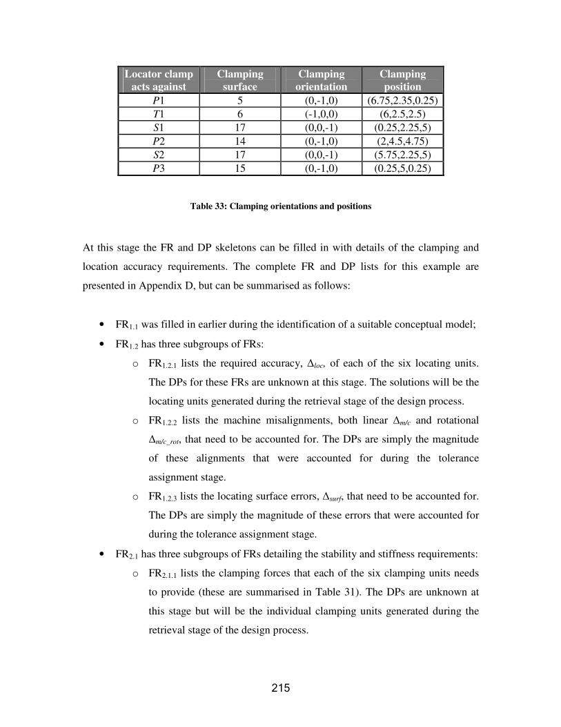
Locator clamp acts against

Clamping surface

Clamping orientation

Clamping position

P1 5 (0,-1,0) (6.75,2.35,0.25) T1 6 (-1,0,0) (6,2.5,2.5) S1 17 (0,0,-1) (0.25,2.25,5) P2 14 (0,-1,0) (2,4.5,4.75) S2 17 (0,0,-1) (5.75,2.25,5) P3 15 (0,-1,0) (0.25,5,0.25)

Table 33: Clamping orientations and positions

At this stage the FR and DP skeletons can be filled in with details of the clamping and location accuracy requirements. The complete FR and DP lists for this example are

presented in Appendix D, but can be summarised as follows:

• FR1.1 was filled in earlier during the identification of a suitable conceptual model;

• FR1.2 has three subgroups of FRs:

o FR1.2.1 lists the required accuracy, �loc, of each of the six locating units.

The DPs for these FRs are unknown at this stage. The solutions will be the locating units generated during the retrieval stage of the design process.

o FR1.2.2 lists the machine misalignments, both linear �m/c and rotational �m/c_rot, that need to be accounted for. The DPs are simply the magnitude of these alignments that were accounted for during the tolerance

assignment stage. o FR1.2.3 lists the locating surface errors, �surf, that need to be accounted for.

The DPs are simply the magnitude of these errors that were accounted for during the tolerance assignment stage.

• FR2.1 has three subgroups of FRs detailing the stability and stiffness requirements:

o FR2.1.1 lists the clamping forces that each of the six clamping units needs to provide (these are summarised in Table 31). The DPs are unknown at

this stage but will be the individual clamping units generated during the retrieval stage of the design process.

!�9�

o FR2.1.2 lists the stiffness required at each locating and clamping point (these are presented in Table 32). The DPs are unknown at this stage but

will be the individual clamping units generated during the retrieval stage of the design process.

o FR2.1.3 lists the need for each clamp to contact the workpiece. The relevant DPs are the clamping coordinates detailed in Table 33.

o FR2.1.4 lists the clamping directions required at each clamping position. The DPs are the workpiece surfaces upon which the clamps act (as

detailed in Table 33).

*�*�*�*�!�#�'� �� %�� /!�#�'� �� %�� /!�#�'� �� %�� /!�#�'� �� %�� / � �� , �!�� , �!�� , �!�� , �!��

Before the individual locating and clamping units can be generated, the design preferences need to be defined. A detailed description of the process by which these are

generated and some examples are described in section 4.3.2.1 but to recap there are four basic stages to defining design preferences:

• define the global constraint attributes that solutions are to be evaluated against;

• specify the acceptable range of performance that is sought of a design for each of those attributes;

• generate the utility curve for each constraint attribute that specifies the utility of

different values of performance within the accepted range;

• determine the scaling constant for each constraint attribute, which is a measure of

the importance of one attribute relative to the others.

For this example, five constraint attributes are considered. These are fixture cost, weight, loading time, assembly time, and unloading time. The utility curves for each constraint

attribute are presented in the following figures. The original curves obtained from the user are presented together with the cubic approximations used by the CAFixD method in

its utility calculations. As the figures indicate there is a close match between this cubic

!�:�

approximation and the curves entered by the user. Table 34 details the scaling constant (ki) for each individual attribute and the overall scaling constant, K.

Figure 118: Utility curve for fixture cost

Figure 119: Utility curve for weight

0

0.1

0.2

0.3

0.4

0.5

0.6

0.7

0.8

0.9

1

8 9 10 11 12

weig ht ( lb )

U t il it y

User value Cubic approximation

0

0.1

0.2

0.3

0.4

0.5

0.6

0.7

0.8

0.9

1

35 37 39 41 43 45

C o st ( $)

U t il it y


!�<�

Figure 120: Utility curve for loading time

Figure 121: Utility curve for assembly time

0

0.1

0.2

0.3

0.4

0.5

0.6

0.7

0.8

0.9

1

35 36 37 38 39 40

A ssemb ly t ime ( minut es)

U t i l i t y

User value Cubic appr oximation

0

0.1

0.2

0.3

0.4

0.5

0.6

0.7

0.8

0.9

1

2 2.5 3 3.5 4

lo ad ing t ime ( minut es)

U t il i t y


!�=�

Figure 122: Utility curve for unloading time

Constraint attribute Scaling constant value

Cost 0.67 Weight 0.35

Loading time 0.23 Assembly time 0.54 Unloading time 0.29

Overall -0.9262283

Table 34: Individual scaling constants ki and overall scaling constant K

The first step of the retrieval process is to determine which cases in case library 2 are suitable for use within the retrieved conceptual model. For simple plane 3-2-1 locating

(variation 3) where no chip shedding requirements have been specified, and there are no complex issues related to the workpiece geometry there are few restrictions on which

cases can be used other than ensuring that both the basic function type (locating or stiffness) and direction of action (vertical or horizontal) are satisfied.

Table 35 presents a sample of the results from the functional similarity-based retrieval

stage. For each locating and clamping point, possible DPs are listed which can

0

0.1

0.2

0.3

0.4

0.5

0.6

0.7

0.8

0.9

1

2 2.5 3 3.5 4

U nlo ad ing t ime ( minut es)

Ut il i t y

User value Cubic appr oximation

!!> �

qualitatively (but not quantitatively) satisfy the appropriate FRs associated with each point. That is they are capable of providing a certain stiffness capability in the correct

direction, but may not in their current form be able to offer the correct magnitude of stiffness. The adaptability-based retrieval stage of the design process will determine how

and if they can be modified and will pick the design solution for each FR or group of FRs that is most in keeping with the design preferences.

Locating/clamping point Possible DP Possible DP P1 VL011C1 VL012C1 T1 HL013C1 HL013C2 S1 HL013C1 HL013C2 P2 VL011C1 VL012C1 S2 HL013C1 HL013C2 P3 VL011C1 VL012C1

Clamp against P1 VC0132C1 VC022C1 Clamp against T1 HC021C1 HC022C1 Clamp against S1 HC021C1 HC022C1 Clamp against P2 VC0132C1 VC022C1 Clamp against S2 HC021C1 HC022C1 Clamp against P3 VC0132C1 VC022C1

Table 35: Output of results from functional similarity-based retrieval

The first stage of this part of the process is to generate a qualitatively complete design

and compute its associated performance values for each of the global constraint attributes. This design is used as an initial reference point for comparing designs. The

highlighted designs in the second column of Table 35 are randomly chosen as this initial design. The case library holds each of these units performance with regard to the global

constraint attributes, and these are displayed in Appendix E. Summing these numbers provides the attribute performance values for this initial, which are listed in Table 36.

!!��

Attribute Performance level Cost ($) 38.64

Weight (lb) 9.219 Loading time (mins) 3.0999

Assembly time (mins) 37.56 Unloading time (mins) 2.55

Table 36: Attribute performance values for initial design

The retrieval process continues by picking each candidate DP in turn and repairing it to

satisfy the FR or group of FRs for which it is being considered. Each method of repair for a particular DP is instigated and evaluated by comparing the ability of the repaired design

to meet the design preferences. Consider as an example the DP VC0132C1 whose details were presented in section 4.4.1. This is a vertical clamp considered as a candidate for

clamping against locating point P1. It has two FRs associated with it – stiffness and clamping force. Its current performance values are:

• stiffness of 17765 lb/in, and;

• clamping force of 35 lb.

The requirements for the current fixture problem are:

• stiffness of 29933 lb/in;

• clamping force of 50 lb.

Thus the design requires adaptation. To modify the stiffness of the clamp there are three possible adaptation strategies:

• modify the thickness of the clamp elements using the strap_thickness_adapt( )

strategy;

• modify the width of the clamp components using the strap_width_adapt( ) strategy;

!!!�

• modify the clamp material using the strap_material_adapt( ) strategy.

Testing of the modification module is performed by the

strap_clamp_third_order_disp_func( ) test module. The first two adaptation strategies share a common control module, dimension_control( ), whilst the material modifications

are supervised by the material_control( ) module.

To modify the clamping force there is only the strap_torque( ) adaptation strategy in which the torque_calc_third_order( ) directly calculates the torque required to produce

the desired clamping force on the workpiece.

The first adaptation method to be invoked alters the thickness of the clamp elements using the alter_ thickness( ) modification module. The control module makes an initial guess at the required thickness change (0.1 inches) which is then implemented by the

modification module. Consider for example element 4 of the clamp, presented in Figure 123a. Element 4 contains a slot into which a mating element (a cylindrical element) from

the work limb of the clamp fits. When altering the thickness of element 4 from 0.5 to 0.6 inches, the same change will also apply to the connecting cylindrical element from the

work limb. Thus the slot width on element 4 must be increased to be able to accept this mating element. The width of element 4 must also be increased to account for the

increase in slot width. This results in the modified dimensions of element 4 presented in Figure 123b. All of the elements within the clamp undergo similar forms of modification

and when this is complete the testing module is called to determine the likely behaviour of the clamp when subjected to the machining forces.

The required stiffness of the clamp is based upon the machining forces and the allowed

displacement, and the test module calculates the likely displacement of the clamp rather than the stiffness itself. Initially the forces on the work and fulcrum limbs are calculated

by applying the equilibrium conditions on the beam for both the real and virtual force systems. Figure 124 presents the calculated real and virtual forces. These forces are then

used to calculate the internal forces acting on each element (see Figure 125). The

!!#�

displacement of a single element can then be calculated using the virtual work method, thus for element 4 which is subject to bending and shear dispalcements:

44

4442

44

444

2

AGLVvf

dxIEMmd s

x

s

+= �

This is repeated for all elements and their respective displacements summed to determine

the displacement of the clamp at the workpiece interface.

Figure 123: Element 4 a) before and b) after modification

0.5 inches

0.3 inches

0.6 inches

0.5 inches

View A

View A

0.5 inches

0.4 inches

0.7 inches

0.6 inches

View A

View A

a) before modification

a) after modification

Slot

!!&�

Figure 124: Calculating Ff and Fw

Figure 125: Free body diagram for element 4

The control module then evaluates the modified design and determines a future course of

action. The key factor used during the control process is the polarity change of calc_disp

– des_disp (this is the calculated displacement – the design displacement). The dimension

change sent to the modification module is modified by a step value: i.e., dim_change =

dim_change + step. Whenever a polarity change occurs, the step used in the dimension

change is decreased by dividing it by 10 and reversing its polarity. Table 37 presents the manner in which the control module converges on a solution by

controlling the value of the step change. After each polarity reversal (represented by the highlighted rows) the step change is altered. Eventually, the clamp is successfully

repaired when a dimension change of +0.09678089 inches is applied to the thickness of

M4

V4 = 200 lb

Fc = 200 lb

x2

m4

v4 = 1 lb

fc = 1 lb

x2

Real force system:

Element 4

s s

Virtual force system:

Ff = Fc * L2 / L1 = 266.67 lb ff = fc * L2 / L1 = 1.33 lb

Fw = Fc + Ff = 466.67 lb fw = fc + ff = 2.33 lb

elem2 elem1

L2 = 2 inches L1 = 1.5 inches

Fw

Fc Ff

!!*�

the clamping elements. In practice this level of accuracy of a dimension change is not practical, but is adopted here to illustrate how a solution is reached.

Dimension change

Applied step value

Calculated displacement

Design displacement

calc_disp – des_disp Success

0 - 0.011258 0.006681 0.004576 No 0.1 0.1 0.006578 0.006681 -0.0001 No

0.09 -0.01 0.006907 0.006681 0.000226 No 0.091 0.001 0.006873 0.006681 0.000192 No 0.092 0.001 0.00684 0.006681 0.000158 No 0.093 0.001 0.006806 0.006681 0.000125 No 0.094 0.001 0.006773 0.006681 9.13E-05 No 0.095 0.001 0.00674 0.006681 5.83E-05 No 0.096 0.001 0.006707 0.006681 2.55E-05 No 0.097 0.001 0.006674 0.006681 -7.1E-06 No

0.0969 -0.0001 0.006678 0.006681 -3.9E-06 No 0.0968 -0.0001 0.006681 0.006681 -6.2E-07 No 0.0967 -0.0001 0.006684 0.006681 2.63E-06 No

0.09671 0.00001 0.006684 0.006681 2.31E-06 No 0.09672 0.00001 0.006683 0.006681 1.98E-06 No 0.09673 0.00001 0.006683 0.006681 1.66E-06 No 0.09674 0.00001 0.006683 0.006681 1.33E-06 No 0.09675 0.00001 0.006682 0.006681 1E-06 No 0.09676 0.00001 0.006682 0.006681 6.79E-07 No 0.09677 0.00001 0.006682 0.006681 3.53E-07 No 0.09678 0.00001 0.006682 0.006681 2.81E-08 No 0.09679 0.00001 0.006681 0.006681 -3E-07 No

0.096789 -0.000001 0.006681 0.006681 -2.6E-07 No 0.096788 -0.000001 0.006681 0.006681 -2.3E-07 No 0.096787 -0.000001 0.006681 0.006681 -2E-07 No 0.096786 -0.000001 0.006681 0.006681 -1.7E-07 No 0.096785 -0.000001 0.006681 0.006681 -1.3E-07 No 0.096784 -0.000001 0.006681 0.006681 -1E-07 No 0.096783 -0.000001 0.006681 0.006681 -6.9E-08 No 0.096782 -0.000001 0.006681 0.006681 -3.7E-08 No 0.096781 -0.000001 0.006681 0.006681 -4.4E-09 No

0.09678 -0.000001 0.006682 0.006681 2.81E-08 No 0.0967801 0.0000001 0.006681 0.006681 2.49E-08 No 0.0967802 0.0000001 0.006681 0.006681 2.16E-08 No 0.0967803 0.0000001 0.006681 0.006681 1.84E-08 No 0.0967804 0.0000001 0.006681 0.006681 1.51E-08 No 0.0967805 0.0000001 0.006681 0.006681 1.19E-08 No 0.0967806 0.0000001 0.006681 0.006681 8.61E-09 No 0.0967807 0.0000001 0.006681 0.006681 5.35E-09 No 0.0967808 0.0000001 0.006681 0.006681 2.1E-09 No 0.0967809 0.0000001 0.006681 0.006681 -1.2E-09 No

0.09678089 -0.00000001 0.006681 0.006681 -8.3E-10 Yes

Table 37: Modification results for strap_thickness_adapt( ) strategy (inches)

!!9�

Once a successful solution has been achieved, the constraint attribute performance values can be determined for the modified unit, as illustrated in Table 38.

Attribute Original clamp performance

levels

Modified clamp performance

levels Cost ($) 1.83 2.18

Weight (lb) 1.1996 1.5624 Loading time (mins) 0.583 0.583

Assembly time (mins) 4.82 4.82 Unloading time (mins) 0.45 0.45

Table 38: The updated constraint attributes for the clamp

These can then be incorporated into the performance values for the overall fixture design

and the utility of the new design (which has the repaired clamping unit in it) calculated. The utility for each individual performance constraint is presented in Table 39, and the

overall utility can be determined using the multiplicative as described in section 4.3.3.2.2 to yield an overall utility of 0.765965.

Attribute Original fixture

performance levels

Updated fixture

performance levels

Individual attribute

utility

Cost $ 38.64 $ 39.03 0.377664 Weight 9.219 lb 9.608299 lb 0.296877

Loading time 3.0999 mins 3.0999 mins 0.706441 Assembly time 37.56 mins 37.56 mins 0.750127 Unloading time 2.55 mins 2.55 mins 0.777805

Table 39: The updated attribute performance values for the modified fixture

The process is then repeated for the second adaptation strategy in which the width of the clamp elements is subject to modification. However, as the calculated displacement

results detailed in Table 40 show, this adaptation strategy failed. Up until a dimension change of 0.7 inches there was a steady decrease in the displacement suffered by the

!!:�

clamp due to machining forces. However when the dimension change was 0.8 inches, the displacement increased. The cause of this is the fact that for a dimension change of 0.8

inches, the length of the beam has to increase between the work and fulcrum limbs to prevent them from colliding with one another. Extending the beam increases the bending

displacement of the beam. In this case the detrimental effect of increasing the beam length L1 has been greater than the beneficial effect of increasing the width of the

element. After three consecutive increases have been recorded in the calculated displacement, the control module aborts the adaptation strategy as a successful solution is

deemed unlikely.

Dimension change

Calculated displacement

Design displacement

Calc_disp – des_disp

Improvement on last change

Success L1

0 0.011258 0.006681 0.004576 - No 1.5 0.1 0.010547 0.006681 0.003866 Yes No 1.5 0.2 0.010146 0.006681 0.003464 Yes No 1.5 0.3 0.009885 0.006681 0.003203 Yes No 1.5 0.4 0.009701 0.006681 0.003019 Yes No 1.5 0.5 0.009563 0.006681 0.002881 Yes No 1.5 0.6 0.009456 0.006681 0.002774 Yes No 1.5 0.7 0.00937 0.006681 0.002688 Yes No 1.5 0.8 0.009769 0.006681 0.003088 No No 1.6 0.9 0.010182 0.006681 0.003501 No No 1.7 1 0.010602 0.006681 0.00392 No No 1.8

Table 40: Testing results for the alter_width( ) modification module (inches)

The third adaptation strategy involves altering the material from which the unit is

constructed using the material_modification( ) module. The control module is aware of four candidate materials and instructs the modification module to implement them one at

a time. Each material is tested and the results are presented in Table 41. Only one material change resulted in a successful clamping unit. The updated constraint attributes

performances for the clamping unit are provided in Table 42 and those values for the updated fixture design as a whole are outlined in Table 43. The utility associated with this

adaptation strategy is 0.634513.

!!<�

Figure 126: Limitations on modifying the work and fulcrum limbs

Material Calculated displacement (inches)

Design displacement

(inches) Success

Stainless Steel 1304 0.011258 0.006681 No

Steel A36 0.010507 0.006681 No Tungsten 0.005431 0.006681 Yes

Steel 1020 0.010507 0.006681 No

Table 41: Displacment results for different materials

Attribute Original clamp

performance levels

Modified clamp

performance levels

Cost ($) 1.83 102.34 Weight (lb) 1.1996 2.893

Loading time (mins) 0.583 0.583 Assembly time (mins) 4.82 4.82

Unloading time (mins) 0.45 0.45

Table 42: The updated constraint attributes for the clamp

0.4 in

L1 = 1.5 in

0.4 in 0.7 in

Maximum change that can be added without extending L1.

!!=�

Attribute Original fixture

performance levels

Updated fixture

performance levels

Individual attribute

utility

Cost $ 38.64 $ 139.19 0 Weight 9.22 lb 10.939 lb 0.055786

Loading time 3.099 mins 3.099 mins 0.706441 Assembly time 37.56 mins 37.56 mins 0.750127 Unloading time 2.55 mins 2.55 mins 0.777805

Table 43: The updated attribute performance values for the modified fixture

The results for each adaptation strategy are compared in Table 44. Only strategies 1

(thickness alteration) and 3 (material alteration) resulted in successful design solutions. Altering the width of the clamping unit failed to return a working design. Of the two

successful strategies, the thickness alteration returns the design with the highest utility and this would be chosen as the final means for attaining the required stiffness. Appendix F presents the updated drawings for the clamping unit.

Adaptation strategy Utility Alter unit thickness 0.765965

Alter unit width 0 Alter unit material 0.634513

Table 44: Comparison of the utility of each adaptation strategy

Figure 127 illustrates the adaptation mapping layout for the stiffness FR/DP combination

for the clamping unit. In the adaptation mapping layout:

• FR2.1.1.1 is the stiffness required of the clamp (29933 lb/in);

• DP2.1.1.1a is the candidate clamping unit VC0132C1;

• PV2.1.1.1a.1 is the thickness dimension change implemented using the

alter_thickness( ) modification module;

!#> �

• PV2.1.1.1a.2 is the width dimension change implemented using the alter_width( )

modification module;

• PV2.1.1.1a.3 is the material change implemented using the alter_material( )

modification module;

• RelFR2.1.1.1a is the relationship between the FR and DP (this is the qualitative

relationship established during the functionality-based retrieval stage when clamping units that could provide a vertical stiffness were sought);

• RelDP2.1.1.1a.1 is the relationship that determines how the thickness design change

affects the FR performance of the DP (this includes the control (dimension_control( ) and strap_clamp_third_order_disp_func( ) control and

testing modules of the thickness adaptation strategy);

• RelDP2.1.1.1a.2 is the relationship that determines how the width design change

affects the FR performance of the DP (this includes the control (dimension_control( ) and strap_clamp_third_order_disp_func( ) control and

testing modules of the thickness adaptation strategy);

• RelDP2.1.1.1a.3 is the relationship that determines how the material design change

affects the FR performance of a DP (this includes the material_control( ) and strap_clamp_third_order_disp_func( ) control and test modules of the material

adaptation strategy).

The remaining FR for this unit is the clamping force FR. Currently the clamp provides a force of 35 lb, but the requirement is for 50 lb so the control module calls on the torque_

calc_third_order( ) function to calculate the torque required at the bolt on the work limb. This modification results in no change to the attribute performances.

Thus for this DP the returned strategies are:

• Stiffness adaptation strategy: strap_thickness_adapt( );

• Clamping force adaptation strategy: strap_torque_ third_order( );

• The returned utility for this DP/adaptation strategy combination is 0.7687858.

!#��

Appendix F presents the drawings for the updated clamp. The process is repeated for the remaining DPs returned by the functional similarity-based retrieval stage, and the

DP/adaptation strategy with the highest utility value is chosen as the final solution for this particular group of FRs.

Figure 127: The adaptation mapping layout for this FR/DP combination

*�*�*�*�####�'� %�� '� %�� '� %�� '� %��

This chapter has presented two examples. One illustrated the manner in which case knowledge is held in case library 2 and the second how a fixture unit is retrieved from the

second case library during adaptability-based retrieval. This second example also

FR2.1.1.1

DP2.1.1.1a

PV2.1.1.1a.2

PV2.1.1.1a.3

PV2.1.1.1a.1

RelDP2.1.1.1a.1 RelFR2.1.1.1a

RelDP2.1.1.1a.2 RelDP2.1.1.1a.3

C12

C13

C10

C11

C8 C9

C1

C2

Key: Input/output;

Local constraint limit affecting PV; PV affecting global constraint attributes; PV affecting other parameters

U(X) = 0.77

U(X) = 0 U(X) = 0.63

(For simplicity only 2 global constraint attributes are illustrated)

Element parameters affected by this design change

!#!�

illustrated how the CAFixD method supports the setup planning, fixture planning, unit design, and verification phases of fixture design.

Adaptation strategies play a crucial role in the adaptability-based retrieval stage.

Evaluation of strategies is based heavily upon the wishes of the designer, who specifies design preferences in the form of utility curves. This adds a dynamic element to the

design process in which the method has the ability to respond directly to design preferences. Thus given the same technical problem in terms of workpiece geometry, the

method can respond in different ways to different users through the adoption of different adaptation strategies. In this way the method seeks to support the design process rather

than control it by allowing the preferences of the user to guide decision making throughout the design tasks. Thus the modus operandi of the method is to support the

designer using an understanding of the design preferences, rather than trying to impose a will of its own on the user. The designer remains the active party during design, and the

method is a tool that reacts to the designer’s wishes.

!##�

�� 9999��, �� "� %� �� , �� "� %� �� , �� "� %� �� , �� "� %� ��

A computer tool, called CAFixD, has been developed to demonstrate the methodology detailed in chapter 4. This chapter focuses on issues associated with creating this software

implementation. An overview of the system is presented in section 6.1, followed by a discussion of the internal information flows, knowledge bases, and data formats used for communication with other CAD tools, as well as the system interface design.

9999��, �� ( %� �%�� , �� ( %� �%�� , �� ( %� �%�� , �� ( %� �%��

CAFixD has been developed using the Visual C++ language in conjunction with Tidestone Formula 1 Workbook Designer. Workbook Designer is a spreadsheet design

tool and this spreadsheet capability is used to simplify information passing within CAFixD. It also acts as a convenient means of displaying system outputs and information

to the user. Code written in the Visual C++ language controls the execution of CAFixD.

Overall, CAFixD has been developed as a stand-alone program that communicates with various other CAD tools and the user to gather information as and when it is required.

The purpose of CAFixD is to process this information and use it to generate a fixture design, and then pass on the details of this fixture design to a CAD package that will

create the design drawings. Figure 128 illustrates the overall relationship with other systems. CAFixD communicates with both CAD and Computer-aided Process Planning

(CAPP) systems. CAPP systems generate the machining information for a workpiece. This information includes the machine tool type, details of the machining processes the

workpiece will undergo, the cutting toolpath, and so on. One-way communication exists between the CAPP system and CAFixD, whilst two-way communication exists between CAFixD and the CAD system. CAFixD receives from the CAPP system information

relating to machining processes the workpiece will undergo, such as machining forces and machine tool tolerances. CAFixD also receives workpiece information from the CAD

system that details workpiece surfaces, features (these are the surfaces to be machined),

!#&�

dimensions, and tolerances. Together, these two sources of information are used to generate a conceptual fixture design and to define the list of FRs for which a design

solution is sought.

To aid the detail design stage, CAFixD receives existing fixture designs from case library 2, which is contained within CAFixD. However a link exists between each case in the

case library and the drawings of the case which are held in the CAD system. The CAFixD case library holds only the completed case and element schemas for a particular

case, but does not contain the actual unit drawings. These are held within the CAD system, and a link exists between the CAFixD and CAD representations of units that

identifies which CAD drawings and CAFixD cases are related to each other.

Figure 128: CAFixD system overview

Generate list of functional requirements and constraints

Create utility curves for each constraint

Perform functional similarity retrieval

Determine required modifications

Implement adaptation strategy

Test case

Evaluate adapted case against constraints

Case library 1

Case library 2

Workpiece CAD model, tolerance information, machining information

Design solution

Utility analysis knowledge store

Domain knowledge

constrains search through

CAFixD

I N T E R F A C E

CAD/ CAPP

systems

Key:

External information transfer

External link

!#*�

To the CAD system, CAFixD sends a list of design modifications that are required to fix a design, which are subsequently implemented by the CAD system. This is the sole

external output of CAFixD, but there are also two internal outputs:

1. the completed case and element schema for the new design solution is added to the case library;

2. the utility curves generated through the design process may also be stored in the utility analysis knowledge base (the decision to store these curves is left to

the discretion of the user).

9999�!��, �� "�!��, �� "�!��, �� "�!��, �� "� ��

A series of knowledge sources are used to support the operations performed by CAFixD.

These sources are all contained within the CAFixD system. There are three sources, each of which may contain either declarative or procedural knowledge, or a combination of

both. The three knowledge bases are the case base, the domain knowledge base, and the utility analysis knowledge base. Figure 129 illustrates a partial breakdown of the

knowledge source hierarchy.

The case base contains the two case libraries, both of which are discussed in some detail in section 4.1. The utility analysis base contains execution knowledge in addition to previous design preferences held in the form of utility curves and scaling constants.

These previous design preferences may be recalled and used again by the designer. It is also possible to edit existing curves and scaling constants before reuse. This feature is

intended to simplify using the utility analysis approach. The process of generating utility curves can be a laborious process and is the main reason that the approach is not widely

adopted in the engineering design community. CAFixD however allows the user to recall old curve sets and modify them. A simple modification may be to stretch the curve by

extending the acceptable performance range, as illustrated in Figure 130. Alternatively, the shape of the curve can be altered using the standard lottery question process. This

!#9�

however is time consuming, so the ideal approach is to have a selection of previous curves that exhibit a wide variation in curve shape. The designer can then pick the desired

shape and then simply modify the acceptable performance range.

Figure 129: Databases that support CAFixD operation

The execution knowledge base contains knowledge of how to control the lottery question

process and the utility curve generation store contains knowledge for generating the equivalent function of the curve. In CAFixD all curves are approximated to cubics. The

evaluation knowledge base contains knowledge on how to determine the overall utility of a fixture design and how to evaluate different DP/adaptation strategy combinations.

CAFixD knowledge base

Domain knowledge base

Case base Utility analysis knowledge base

Case library 2

Case library 1

Design preferences knowledge

base

Execution knowledge

base

Utility curves base

Scaling constants

ki base

Lottery question

generation knowledge

base

Utility curve/ scaling

constant generation knowledge

base

Evaluation knowledge

base

!#:�

Figure 130: Modifying a utility curve

The remaining base contains the domain knowledge that supports both the FR generation and retrieval stages. Its contents, detailed in Figure 131, assist both the conceptual and

detail design phases. The indexing knowledge base assists both the selection of a suitable locating principle design from case library 1 and subsequent refinement of the FR

skeleton associated with the locating principle. Initially the DSMRG knowledge base is used to generate the DMSRG for the workpiece. This DMSRG (introduced in section

2.1.1) is a set of graphs that illustrate the relationship between the datum and machining surfaces in a particular setup. The DMSRG is subsequently analysed using knowledge

from the locating knowledge store to determine the locating surfaces, subsequent conceptual model, locating point distributions, and position coordinates.

The tolerance analysis knowledge base supports refinement of the FR/DP skeleton by

using the:

• tolerance type and sensitivity analysis knowledge bases to perform the sensitivity

analysis;

Initial range Attribute performance

Utility

Extended range

Initial curve

Extended curve

!#<�

• tolerance type and tolerance analysis knowledge bases to perform the tolerance

analysis;

• tolerance assignment knowledge bases to support the tolerance assignment stage

of the design process.

Applying knowledge from these sources results in the completion of the first group of FRs, which state the locating requirements for a workpiece. The force analysis

knowledge base is used to refine the second group of FRs related to fixture stability. This knowledge helps determine the clamping orientations, surfaces, and coordinates. In

addition it is also used to calculate the required stiffness at each locating and clamping point, and the required clamping forces.

Figure 131: The domain knowledge database

The learning knowledge base assists the learning process with CAFixD. The addition

knowledge base is used to control the process of storing new cases in the case library (in terms of where they should be put). The maintenance knowledge base is used to govern

Domain knowledge base

Learning knowledge base Indexing knowledge base Retrieval knowledge base

Locating knowledge

base store

Tolerance knowledge

base store

Force analysis knowledge

base

Tolerance assignment knowledge

base

Sensitivity analysis

knowledge base

Tolerance analysis

knowledge base

Tolerance type

knowledge base

DMSRG knowledge

base

Maintenance knowledge

base store

Addition knowledge

base

Adaptation knowledge

base

FR/DP mapping

knowledge base

Adaptation strategy

knowledge base

Adaptation strategy selection

knowledge base

Modification module

knowledge base

Testing module

knowledge base

Control module

knowledge base

Constraint attribute metric knowledge base

!#=�

the maintenance of case library 2 by evaluating the usefulness of cases and determining those which are to be removed.

The retrieval knowledge base contains knowledge relating to both the functional

similarity-based and adaptability-based retrieval processes. The former is a rule base used to determine which DPs in case library 2 can qualitatively satisfy each FR, and which

FRs have common solutions. The adaptation knowledge base contains the adaptation strategies and the rules for selecting particular strategies. The adaptation strategy

knowledge source contains the modification, testing, and control modules used in different adaptation strategies. The constraint attribute metric knowledge base contains

the heuristic knowledge used to calculate a unit’s performance values for each global constraint attribute.

9999�#�� #�� #�� #��

The operation of CAFixD can be decomposed into four main processes. Initially the fixture conceptual design and the design FRs are generated. Following this the design

preferences are recorded, which includes defining the global constraint attributes that apply for a given design situation and utility curves for each of those attributes. In the

third process, the two stage case retrieval procedure is executed. Finally, the design modification file is created and maintenance of the case base is performed. Presented in the following four sections are the information flows for each process, which highlight

where the knowledge required for the completion of each process is obtained.

9999�#��. �� #��. �� #��. �� #��. �� "� �� 4�� "� �� 4�� "� �� 4�� "� �� 4 � � � ��

CAFixD requires input from external sources when developing the conceptual design using the process depicted in Figure 132. In this design stage, CAFixD is defining the

fixture design problem statement, hence the need for considerable external input.

!&> �

Information is sought from the CAD system regarding the workpiece information, from the CAPP system regarding machining process data, and from the user regarding specific

requirements (i.e., which ergonomic FRs are required – as has been stated previously, these requirements cannot be generated automatically and need to be specifically

requested by the designer). The output from this stage is the completed FR list detailing all locating, stability, and ergonomic requirements.

9999�#�!�. �� !��#�!�. �� !��#�!�. �� !��#�!�. �� !��4 � � � �� / ��, �� %� �� 4 � � � �� / ��, �� %� �� 4 � � � �� / ��, �� %� �� 4 � � � �� / ��, �� %� ��

The generation of utility curves and scaling constants (Figure 133) is conducted

interactively with the user. Lottery questions are generated for each FR and constraint, and the user response to each question is monitored and used to guide the lottery question

generation process. The utility curves are then generated and stored in the system for use during case retrieval. The process is repeated to determine the scaling constants for each

global constraint attribute. This is a fairly time consuming process, thus there is also the option for the user to simply choose a set of previously stored curves and either use them

directly or modify them as desired.

9999�#�#�. �� #��#�#�. �� #��#�#�. �� #��#�#�. �� #��'� �� %� ��'� �� %� ��'� �� %� ��'� �� %� ��

From the retrieval stage onward the system requires no further user input and draws from

its own knowledge sources to complete the design process, as illustrated in Figure 134. The functional mapping knowledge is used to identify cases within case library 2 that are

able to satisfy either single FRs or groups of FRs. An initial reference design is then generated from these candidate cases and the global constraint attribute performance

values for that design calculated using knowledge from the constraint metric base.

!&��

Figure 132: Generating a conceptual design

External inputs Process Internal knowledge base

CAD model, machining

information Identify locating

directions DMSRG and

locating knowledge bases

CAD model Identify locating surfaces Locating

knowledge base

CAD model Identify locating principle Locating

knowledge base

Retrieve FR

skeleton set for locating principle

Case library 1,

locating knowledge base

CAD model Refine location FRs

Sensitivity analysis, tolerance analysis,

tolerance assignment, and tolerance type

knowledge bases

CAD model Refine stability FRs

Force analysis, tolerance

assignment knowledge bases

User input Select ergonomic FRs

!&!�

Adaptability guided retrieval is the most intensive operation CAFixD performs, where the system attempts to see into the future by determining both what modifications are

required and also their likely impact. The adaptation strategy selection knowledge identifies the relevant strategies that can be used to fix designs, and the implementation

of these strategies is controlled by their control modules. Modifications are implemented using knowledge from the modification modules base and subsequently tested. The

constraint metric knowledge is used to calculate the attribute performance values of the repaired design and the evaluation module from the utility analysis knowledge base

evaluates and ranks the DP/adaptation strategy combinations based upon the updated constraint attributes for the new fixture design. The highest ranked DP/adaptation

strategy combinations for each FR or group of FRs are then chosen as the final design solutions.

9999�#�&�. �� &��#�&�. �� &��#�&�. �� &��#�&�. �� &��"� �� $� � �� "� �� $� � �� "� �� $� � �� "� �� $� � �� ++++� � �� $� �� $� �� $� �� $� ��

The final operations that CAFixD performs are to generate the modification file that is

passed onto the CAD system, and to maintain the case library. The fixture design “assembled” during the adaptability-based retrieval stage is proposed as the final design:

i.e., this complete fixture design consists of the top ranked (as determined by the utility analysis evaluation module) individual design cases retrieved from case library 2. The

modifications for that design are formulated and the modification file generated using the modification knowledge from the adaptation knowledge base.

The system then adds the individual units from the design to the appropriate sections of

case library 2. The library is then subjected to maintenance, which is the removal of knowledge that fails to meet the usefulness criteria. This criteria is based upon how often

knowledge is successfully used, and that which is rarely recalled is deleted from the case library, subject to the restrictions described in section 4.2.5 that are designed to ensure a good spread of case knowledge exists throughout the library.

!&#�

Figure 133: Generating utility curves and scaling constants

External input Process Internal knowledge base

User input

Declare relevant global

constraint attributes

User input

Define acceptable

performance ranges

User input Generate utility curves

Lottery question generation, utility

curve/scaling constant generation knowledge

bases (utility curves base if recalling old curves)

User input

Generate single

attribute and overall scaling

constants

Lottery question generation, utility

curve/scaling constant generation knowledge

bases (scaling constants base if recalling old scaling constants)

!&&�

Figure 134: Retrieval based upon functional similarity

External input Process Internal knowledge base

Identify FRs requiring common solutions

Functional mapping

knowledge base

Generate initial reference solution

Constraint attribute metric knowledge base

Identify

adaptation strategies

Adaptation

strategy selection base

Implement adaptation

modification Control module

base

Modify design Modification module base

Test modification Testing module base

Evaluate functional success of

modification

Control module base

Evaluate DP/adaptation

strategy combinations

Modification module store,

constraint attribute metric,

evaluation knowledge base (utility analysis)

Identify final design solution

Evaluation knowledge base (utility analysis)

!&*�

Figure 135: Modification and case-base maintenance

9999�&�"� �� &�"� �� &�"� �� &�"� ��

Section 5.3 highlighted that CAFixD communicates with other CAD/CAM systems. For

successful communication to be possible, specific formats for the transfer of information between systems need to be defined. This section outlines the formats in which

information is passed, as well as defining the nature of that information.

External party Process Internal knowledge

base

Generate modification file Modification module

knowledge base

CAD system Pass file onto CAD system

Add new cases to case library 2 Case library 2

User specify Define useful knowledge criteria

Identify non-useful knowledge in case

library 2

Maintenance knowledge base, case

library 2

Delete non-useful knowledge from

case library 2

Maintenance knowledge base, case

library 2

!&9�

9999�&��"� �� &��"� �� &��"� �� &��"� �� 7 � � � �� 7 � � � �� 7 � � � �� 7 � � � �� "�� "�� "�� "��, �� , �� , �� , ��

To assist in the generation of the conceptual fixture design (i.e., determination of the locating principle and locating/clamping points), CAFixD requires a significant amount

of knowledge regarding the geometry of the workpiece. Specifically, CAFixD needs a list of the surfaces that comprise a workpiece and subsequent details of those surfaces.

Currently CAFixD supports plane and hole surface types. Typical information required about a surface:

• the surface type;

• the surface identification tag;

• the surface material;

• the surface status (is it a surface that is to be machined, or has been machined, or

has not been and is not due to be machined);

• the number of tolerances existing for a surface;

• the tolerance details (tolerance type, value, and datums);

• position of the local coordinate system of the surface relative to the workpiece coordinate system;

• orientation of the surface normal with respect to the workpiece coordinate system;

• the dimensions of the surface.

The geometric information required for each surface type varies. For a rectangular plane (RPLANE) the position and orientation of the surface’s local coordinate system (LCS)

relative to the workpiece global coordinate system (WCS) are required. The positive z axis of the LCS points directly into the surface. Looking into the surface, the LCS is

located at the bottom left hand corner. The length value acts in the LCS x direction, and the height value in the LCS y direction, as depicted in Figure 136.

!&:�

Figure 136: The geometric data of a rectangular plane

For a hole (HOLE) the position and orientation of the surface’s local coordinate system

(LCS) relative to the global coordinate system (GCS) are required. The LCS is located at one end of the central axis of the hole, with the positive z axis of the LCS pointing

directly into the hole. The diameter and depth of the hole also have to be defined.

Figure 137: The geometric data of a hole

The data needs to supplied in an Excel worksheet and the data file for the workpiece from

the example presented in section 4.4 can be viewed in Appendix G.

WCS

length

x LCS

height

z

GCS LCS

y

x

diameter

length

y

!&<�

9999�&�!�"� �� $� � �� . . ��&�!�"� �� $� � �� . . ��&�!�"� �� $� � �� . . ��&�!�"� �� $� � �� . . ��, �� , �� , �� , ��

To determine the both the fixture stability and locating tolerance requirements, CAFixD requires information regarding the machining processes the workpiece will undergo, as

well as the accuracy of the machine tool itself. The specific machining information required is:

• machine type (e.g., vertical machine tool);

• accuracy along the x, y, and z axes;

• accuracy around the x, y, and z axes;

• machined surface;

• machining operation type;

• tangential and thrust machining forces ;

• toolpath type;

• initial direction of cutting tool.

As with the workpiece information, this data needs to be supplied in the form of an Excel

worksheet, and the machining data for the example presented in section 4.4 can be viewed in Appendix H.

9999�&�#�"� �� "� �� &�#�"� �� "� �� &�#�"� �� "� �� &�#�"� �� "� �� "��, �� "��, �� "��, �� "��, ��

The information required for each design case is held in the form of a case schema with an attached element schema which contains details of the individual elements that

comprise a unit. These are held within case library 2 (again in an Excel spreadsheet) and are a direct replication of the schemas detailed for units in section 4.2.4. A sample

schema for the clamping unit used for the example in section 4.4 is presented in Appendix B.

!&=�

9999�&�&�"� �� $� � �� . � �� &�&�"� �� $� � �� . � �� &�&�"� �� $� � �� . � �� &�&�"� �� $� � �� . � �� "��, �� "��, �� "��, �� "��, ��

The output from CAFixD is a modification file (in Excel format) listing the necessary changes that need to be made to fix a current design. To perform the modifications the

CAD system itself needs to have both an interface file to interpret the CAFixD modification file and a parametric modelling capability to subsequently perform the

modifications on a design case. The CAFixD modification file details changes to:

• the dimensions of an element (length, height, and width);

• the material type of an element;

• the position of an element within a particular limb;

• the connections between elements (including length, diameter, and position of connectors).

A sample output file is presented in Table 45 for element 10 of the repaired clamping unit

created during the example in section 4.4. The full modification file is presented in Appendix I. Element 10 has its length increased from 2 inches to 2.175 inches. All

mating holes are subject to an increase of 0.0875 inches and the mating to connector has an increase in length of 0.0875 inches. The thickness (start_b and end_b dimensions) is

increased to 0.8968 inches, as is the width (start_h and end_h dimensions). The “mate to” connector holes have their diameters increased as a result of the element cross section

dimension changes to 0.112 inches, on an increased diameter offset of 0.673 inches. The “mate from” hole diameter is increased to 0.4968 inches to accommodate the dimension

increase in the connecting fulcrum element, but remains centred within element 10.

!*> �

Element number: 10 Set length to: 2.175 Modify connector hole depth by: 0.0875 Connector hole depth measured from: 'Mating to' surface: Modify connector length by: 0.0875 Modify connector hole depth by: 0.0875 Connector hole depth measured from: 'Mating from' surface: Set start_b dimension to: 0.8968 Dimension measured: Across local central axis Set 'mate to' connector diameter to: 0.1121 Set 'mate to' connector hole diameter to: 0.1121 Set connector offset (mate to) diameter to: 0.6726 Set 'mate from' connector hole diameter to: 0.4968 Set connector offset (mate from) diameter to: 0 Set end_b dimension to: 0.8968 Dimension measured: Across local central axis Set start_h dimension to: 0.8968 Dimension measured: Across local central axis Set end_h dimension to: 0.8968 Dimension measured: Across local central axis

Table 45: The modification list for element 10

Figure 138: Element 10 before modifications

A

View A

Element 10

!*��

Figure 139: Element 10 after modifications

9999�*��, �� *��, �� *��, �� *��, ��

CAFixD is a menu driven system that attempts to guide the user sequentially through the fixture design process. The system accepts user input and then performs setup planning,

fixture planning, unit design, and verification. Information is gathered from the user and other systems through dialogs, processed internally by CAFixD, and then relevant outputs are displayed to the user. CAFixD was created using both Visual C++ and

Tidestone Formula One Version 6. The Tidestone software is a workbook design package that generates spreadsheet applications. This greatly facilitates the transfer of information

to and from Excel worksheets, and is also a useful means of displaying CAFixD outputs to the user during execution. Furthermore, most users will already be familiar with the

layout of a spreadsheet package and should therefore be comfortable with the layout of the CAFixD program and be able to navigate through it with some facility.

The main CAFixD screen is presented in Figure 140. The menu is divided into four main

sections that represent the main stages of the design process. Initially, the design problem

!*!�

must be specified and expressed as a list of functional requirements that the design must satisfy. The designer inputs the workpiece and machining data to allow CAFixD to

process this information, and also specifies which ergonomic FRs and constraints apply. The second stage involves the design preferences in the form of utility curves and scaling

constants. Case retrieval is then performed on the basis of functional similarity and then adaptability, before the new design is subsequently processed (generation of the

modifications file and maintenance of the case base).

As illustrated in Figure 140, there are ten sheets used to display information to the user. The first sheet (Design overview) is used to display an overview of the design and the

design process to the user. Particular information displayed includes:

• the basic locating principle, the locating points, surfaces, and coordinates;

• the sensitivity analysis table;

• the tolerance assignment table;

• the machining forces acting on each locating point;

• all units retrieved during the functional similarity-based retrieval stage;

• the utility analysis results for each FR;

• any features that were not machined in the current setup.

The “FR decomposition” sheet lists the completed FR/DP skeleton for a problem, such as that presented in Appendix D. The “Constraints” sheet lists the global constraint

attributes applicable to the design problem and their respective values. The “Utilities” sheet contains the details of the utility curves and scaling constants for each of the

constraint attributes. The “About CAFixD”, “Instructions”, and “Operation” sheets are information sheets providing various operational details and help with regard to using

CAFixD. The “Solution” sheet contains the completed schemas of the final design solutions for each FR or group of FRs. The “Modification file” sheet contains the

modification lists for each element within each design solution. The final sheet presents a review of the case library status, an example of which is presented in Figure 141.

Shortfalls in the case library 2 knowledge base are highlighted in red, and shortfalls occur

!*#�

when the net number of case example for a case type is less than the minimum acceptable number specified by the user.

Figure 140: The main CAFixD Screen

!*&�

Case Type Total number Cases involved in too few retrievals

Net number

VL011 2 0 2 VL012 1 0 1 VL013 3 0 3 VL021 1 0 1 VL022 2 0 2 VL023 0 0 0 VL024 0 0 0 HL011 1 0 1 HL012 1 1 0 HL013 1 0 1 HL021 1 0 1 HL022 1 0 1 HL023 2 0 2 HL024 0 0 0

COML011 0 0 0 COML012 0 0 0 COML013 0 0 0 COML021 0 0 0 COML022 0 0 0 COML023 0 0 0 COML024 0 0 0

HC011 2 2 0 HC012 0 0 0

Figure 141: The status of case library 2

!**�

::::��

Thus far the objectives of the CAFixD methodology, the method itself, and a worked example of its operation have been presented. This chapter presents a review of how

effective the CAFixD method is with regard to the objectives outlined in Chapter 3. Initially in section 7.1 the contributions of the CAFixD method are presented, followed by an evaluation of its effectiveness, culminating in a number of recommendations that if

implemented would improve the effectiveness of the method.

::::��

Overall the CAFixD approach involves decomposing a design problem into a number of

sub-problems and obtaining solutions for each of those sub-problems, such that a satisfactory design solution is attained that meets the overall design requirement. The

design requirement is rigorously defined by analysing the workpiece geometry, design tolerances, and machining forces. Initially the workpiece design datums are used to select

a suitable conceptual locating model and its skeleton FR set from case library 1. By performing a sensitivity and tolerance analysis, the allowed tolerance allocated to each

locating point within the conceptual model can be determined. These analyses allow the skeleton FR set to be completed and the design process progresses to obtaining individual

units that satisfy the FRs generated for each locating and clamping position.

The complete fixture design is gradually developed one unit at a time in a basic hill climb approach. Identified candidate design cases (DPs) for particular FRs are retrieved from

case library 2 and adaptation strategies are identified that can adapt the design so that it satisfies the new FR. Successful DP/adaptation strategy combinations are then evalauated with regard to how well they satisfy the preferences of the designer. These preferences

relate to the global constraint attribute performance levels for the complete fixture design. Those combinations that best match the design preferences are chosen as the final

solutions, and this process is repeated for each FR. Decision making within this stage of

!*9�

the design process is guided by preferences of the designer. The method reacts to the wishes of the designer and does not seek to impose its own desires upon the design

solution. It provides a means for making decisions but the actual decisions made will be dependent upon the designer’s preferences. In this way the method seeks to support

designers, not replace them.

The contributions of the CAFixD method are argued from two positions. One is from a theoretical standpoint in terms of contributions towards design theory. The second is

from a more application based viewpoint of developing an intelligent tool to assist fixture design.

From a theoretical standpoint, the contributions towards the process of design are mostly

related to CBR and are argued to be:

• The integration of three design theories into a single functioning design method. The CAFixD method is modelled on a case-based reasoning form, but traditional CBR

techniques have been replaced with alternative design theories. In particular axiomatic design is used as the chief means by which cases are indexed, and utility

analysis is used to control the decision making process during retrieval.

• Axiomatic design decomposition is used to overcome the indexing problem inherent

with any CBR approach. The surface attributes of a design problem are considered

customer attributes (in axiomatic design parlance) and are analyzed to determine the specific functions that the design solution must satisfy.

• The use of utility analysis allows designers to express their preferences with greater clarity than possible with standard linear weighting techniques often associated with

CBR techniques.

• Retrieval is split into two stages to overcome the computational issue often associated

with adaptability-based retrieval. Initially functional mapping vets candidates in the case library to identify feasible candidate solutions. Adaptability-based retrieval then

assumes control of generating design solutions by identifying possible means of repairing designs, instigating each repair strategy in turn, and evaluating each repair

!*:�

against the wishes of the designer. Emphasis during retrieval is based upon satisfying the designer’s preferences, and extends beyond just finding something that

functionally satisfies the design problem.

• The “adaptation mapping layout” is proposed as a representation to show both the

relationships between FRs, DPs, and PVs, and the effects of implementing any

particular adaptation strategy (in terms of calculated utility and the effects upon other parts of a DP caused by the implementation of a particular adaptation strategy).

Within the CAFD field, the contributions of the CAFixD method are argued to be:

• The development of a method that can assist all four stages of fixture design.

Specifically: o The CAFixD method can identify multiple setups during setup

planning. o During fixture planning the CAFixD method can identify feasible

locating principles for workpieces, identify surfaces to be used for location and clamping, as well as the coordinates of the contact

points, and provide an initial estimation of the locating tolerances. o During unit design the CAFixD method can generate individual

clamping and locating units based upon an understanding of the allowed deflections of these units. This is achieved through an

analysis of the machining and clamping forces together with the workpiece tolerance requirements.

o During verification, the CAFixD method can confirm if a generated design is capable of satisfying the FRs associated with it by using a solid understanding of how a particular unit behaves. For example

the stiffness analysis uses knowledge of how each fixture unit responds to experienced forces when evaluating if the unit is stiff

enough and will allow the design tolerances to be achieved.

• The generation and use of a comprehensive formulation of the fixturing

requirement to drive the design process. This understanding includes:

!*<�

o workpiece geometry; o workpiece design tolerances;

o workpiece stability; o fixture unit stiffness;

o fixture cost; o fixture usability;

o fixture component collision; o fixture weight;

o workpiece loading and unloading times; o fixture unit assembly times;

• The development of a method for determining the physical structure

individual fixture units should assume. This generation of physical units is based not just upon satisfying workpiece geometry, but also upon the behaviour required of them: e.g., their displacement when subjected to

machining forces.

::::�!�6%� �� !�6%� �� !�6%� �� !�6%� ��

Evaluation of the CAFixD method reveals not only its strengths as detailed in the

previous section but also some aspects to which greater attention could be paid. The first such area relates to optimizing the utility, to which there are two limitations with the

CAFixD method. Currently each adaptation strategy is evaluated in isolation, but an alternative approach might be to consider merging strategies together when searching for

a solution. Consider the example of modifying a vertical unit to satisfy a stiffness requirement. The objective is to find the cheapest solution. A candidate case has the

dimensions presented in Figure 142 and is made of material A, which has a modulus of elasticity of 28E6 lb/in. The unit stiffness is 2.53E6 lb/in.

!*=�

Figure 142: A vertical locating unit

Suppose that the desired stiffness is 6.1E6 lb/in. There are two possible adaptation strategies. One is to alter the cross sectional dimensions of the unit, and the other is to

alter the material type. The available materials are A and B and their properties are listed in Table 46. Of the two strategies, only the dimension modification approach will work if

each strategy is implemented in isolation, as illustrated in Table 47. If however the strategies are combined by altering both using material B and altering the dimensions,

then a unit of satisfactory stiffness can be achieved at a cost below that obtained implementing the dimension adaptation strategy in its own (see Table 47). Thus

combining strategies has resulted in the generation of a cheaper solution.

Material Modulus of elasticity (lb/in) Cost ($/in3) A 28000000 3 B 20000000 1

Table 46: Material properties

t = 0.5 inches

w = 0.5 inches

r = 0.3 inches

l1 = 1 inch

l2 = 0.5 inches

!9> �

Unit Attribute Dimension adaptation strategy

Material adaptation strategy

Combined adaptation strategy

t (inches) 0.7 0.5 0.806 w (inches) 0.7 0.5 0.806 r (inches) 0.5 0.3 0.606 Material

modulus (lb/in) 28E6 20E6 20E6

Stiffness (lb/in) 6.1E6 1.8E6 6.1E6 Cost ($) 1.76 0.29 0.79

Table 47: Results gained by implementing the adaptation strategies

A second aspect concerning optimisation is the effect that the timing of design decisions has on attempts to optimize the design utility. Currently the CAFixD method operates on

a basic hill climb approach where the local optimum DP/adaptation strategy is chosen for a particular FR, and then the retrieval process moves onto obtaining solutions for the next

FR. If presented with two design options at a particular part of the solution progression, then one will be more favorable than the other. However, if the same decision is taken at

a later time during the design phase then the outcome may be different because as the design progresses the location of the design within the acceptable performance range for

each constraint attribute changes and the preferences at one stage of the design vary from those at another.

Consider for example that a choice has to be made between designs A and B to satisfy a

particular FR, both of which make contributions to the performance values of the constraint attributes 1, 2, and 3 for a complete design. For the purposes of the example, it

does not matter what these attributes are, but the design preferences for each of them are important and are illustrated in Figure 143. Attribute 1 is a “less-is-better” attribute

whereas attributes 2 and 3 are “more-is-better” in nature. The contributions of designs A and B to each of these attribute performance values are presented in Table 48.

!9��

Figure 143: Utility curves for attributes 1, 2, and 3

Design Attribute 1 contribution

Attribute 2 contribution

Attribute 3 contribution

A 3 3 2 B 1 1 2

Table 48: Contributions of designs A and B to attributes 1, 2, and 3

As the design solution progresses, the attribute performance values for the complete

design will change as DPs are chosen for each FR. Remember the approach adopted in the CAFixD method is to incrementally build up the complete design solution by finding

individual DP solutions for each FR. Now if a choice is to be made between DPs A and B, then the outcome of that decision will depend upon when the choice is made. Consider

0

0.1

0.2

0.3

0.4

0.5

0.6

0.7

0.8

0.9

1

30 32 34 36 38 40

A t t ribut e 1

U t il it y

0

0.1

0.2

0.3

0.4

0.5

0.6

0.7

0.8

0.9

1

20 22 24 26 28 30

At t r ibut e 2

U t i li t y

00.10.2

0.30.40.50.60.7

0.80.9

1

10 12 14 16 18 20

A t t r ib ut e 3

U t il it y

Scaling constant values are: k1 = 0.5; k2 = 0.5; k3 = 0.1; Overall scaling constant K = -0.2918

!9!�

two design states. One design state is early on in the solution process, and at that time the attribute performance values for the complete design are 31 (attribute 1), 21 (attribute 2),

and 14 (attribute 3). The second design state occurs later on and the performance values for attributes 1, 2, and 3 are 36, 26, and 14 respectively. The two cases are evaluated at

both design states. The results of the utility analysis for design state 1 is presented in Table 49, and that for design state 2 in Table 50.

Attribute Initial

value

Design A

contribution

Total

value

Individual

utility

Design B

contribution

Total

value

Individual

utility

1 31 3 34 0.4 1 32 0.62

2 21 3 24 0.15 1 22 0.05

3 14 2 16 0.6 2 16 0.6

Overall

utility

0.326 Overall

utility

0.387

Table 49: Design state 1 analysis

Attribute Initial

value

Design A

contribution

Total

value

Individual

utility

Design B

contribution

Total

value

Individual

utility

1 36 3 39 0.05 1 37 0.17

2 26 3 29 0.7 1 27 0.4

3 14 2 16 0.6 2 16 0.6

Overall

utility

0.43 Overall

utility

0.34

Table 50: Design state 2 analysis

The important result to note is that at design state 1, DP B is preferable, but at state 2 DP

A returns the highest utility. Thus in its current format the CAFixD methodology is

!9#�

unable to understand and handle the dynamic nature of a design solution. To cope with this problem two major tasks must be undertaken:

1. the total number of design states needs to be identified and defined in terms of the

attribute performance values for each state; 2. each DP/adaptation strategy option for a particular FR has to be evaluated at each

of these design states.

The number of design states is dependent on three items:

1. the number of FRs or groups of FRs for which a solution is sought; 2. the number of candidate DPs for each FR;

3. the number of possible adaptation strategies for each DP.

The number of design states is factorial in nature, and this when added together with the previous suggestion of combining adaptation strategies would result in the need for

significant levels of computation in order to optimize the design solution, but the possibility for expanding the method in this way is feasible, if admittedly complex.

Only limited testing of the CAFixD system has been undertaken to date, and specific

aspects of the approach require greater levels of validation. In particular various sensitivity analyses need to be performed. These relate to several aspects of the method,

but two stand out in particular. The first concerns the utility curves. These curves are currently approximated as cubics and work needs to be done to identify how variation in

the accuracy of these curves affects the design outcome. Specifically, the question to be answered is how accurate do the curves have to be. If they are modelled as linear curves

instead of cubics, then will that result in a different design solution? Secondly the CAFixD method uses a number of heuristic rules to determine the individual

contributions of an adapted design to the global constraint attribute performance levels. Studies need to be performed to determine how accurate these heuristics need to be. For

example, the assembly time heuristic assumes a specific time for each assembly

!9&�

operation. During assembly however, these times may not be accurate for the individual person assembling the fixture. The individual may work more or less quickly than the

recorded heuristic values. If so, then if this inaccuracy had been incorporated into the design process, would a different solution have been proposed? Such studies have yet to

be performed.

Other testing possibilties relate to verifying the accuracy of the unit displacement analysis of clamping and locating units. For example, clamping units are modelled as levers but

this represents an approximation of their behaviour. Calculating the stiffness of a clamping unit is a complex issue, and several research efforts are directed towards

solving this problem (Zheng, 2005). To evaluate the accuracy of the displacement analysis used in the CAFixD method, experiments need to be performed to compare the

measured displacement of a fixture unit with that calculated by the CAFixD method. Depending on the identified accuracy levels, it may be necessary to incorporate a factor

of safety into the displacement analysis procedure used in the CAFixD method.

Another form of necessary testing is to compare the fixture designs obtained using the CAFixD method with those generated by an experienced fixture designer, and attempt to

determine if the design produced using the CAFixD method is better or worse than that of the designer. Given the limitations of the CAFixD software with regard to workpiece

complexity, the workpiece would have to be simple in nature. However, this type of evaluation is very important in determining if the CAFixD method is suited to industrial

use. To be used in industry, the CAFixD method needs to be able to design fixtures that instill confidence in those who will use them.

A particularly helpful feature of the system implementation of the CAFixD method is the

ability to monitor knowledge levels within the case library through the maintenance facility. Importantly, shortfalls in knowledge can be identified. Currently this is as far as

CAFixD goes in terms of evaluating its own knowledge levels but it leaves open the future possibility of the system being able to generate new cases to cover identified

shortfalls. Assuming at least one design case already exists within any particular class

!9*�

type, the adaptation knowledge (in the form of adaptation strategies) can be used to generate new cases. The issue to be addressed relates to controlling this process. The

adaptation strategies all contain a control module designed to satisfy a specific type FR. Thus to use these adaptation strategies, a new facility would have to be added to the

system that would automatically generate FRs that could be passed to the control modules.

Specific challenges in this regard relate to identifying what these FRs should be. One

approach may be to randomly generate FRs until the case levels are at the requisite level and then rely on the maintenance mechanism already present within CAFixD to root out

cases that are of little benefit. A more targeted approach may be to monitor previous FRs and use these as the basis for generating new cases. For example FR requirements in well

populated parts of the library could be copied to sparse areas, and design cases generated to satisfy these FRs. Alternatively if a class type has only two cases in it which satisfy

locating unit stiffness values of 20E6 lb/in and 6E6 lb/in, then previous FR values from other parts of the library could be used to determine if it is worthwhile generating::

• a number of cases with stiffness values lower than 6E6 lb/in;

• a number of cases with stiffness values higher than 20E6 lb/in;

• a number of cases with stiffness values between 6E6 lb/in and 20E6 lb/in;

• a number of cases with stiffness values ranging from below 6E6 lb/in to greater

than 20E6 lb/in.

A related issue to the case library concerns the maintenance mechanism. Currently a blanket, minimum number of cases is required in each class type, but this could be

refined to allow different numbers of cases to be held in different class types. This may be particularly beneficial when working consistently in specific parts of the library. It

may be advantageous to allow, within these high activity zones, an increase (which may be only temporary) in the number of allowed cases to increase the likelihood of finding

the most satisfactory solution during retrieval.

!99�

A second concern with case library 2 is maintaining a diverse range of cases within each class type. The maintenance mechanism can support diversity between class types across

the library by virtue of the fact that each class type must have a minimum number of cases within it before maintainenace is performed. However, within a class type no

diversity is assured as cases are expunged using criterion based solely upon their retrieval success. This criterion does not include consideration of case diversity. Thus some means

of maintining diversity within a class type needs to be determined.

A further refinement may be to offer more guidance when problems occur during design. In the CAFixD software, error messages exist that detail to the user specific problems

with the design, and typically these messages will state the likely cause of the problem and offer high level advice on how to correct it. Common examples include errors

relating to the generation of any negative tolerance assignments. Figure 144 presents a standard error message displayed by CAFixD. CAFixD will inform the user that a

particular tolerance assignment is not achievable due, for example, to the workpiece tolerances or the machine tool accuracy. It does not however fix the problem

automatically, but rather makes suggestions and leaves final decisions to the discretion of the user. An alternative approach might be to assume a more proactive role in fixing the

problems.

Figure 144: An error message displayed by CAFixD

For example, if an unattainable tolerance assignment is observed, CAFixD could automatically attempt to retrieve a machine tool with a suitable level of accuracy from a

database of machine tools. A different approach might be to backtrack through the tolerance and sensitivity analyses to identify the workpiece tolerance that is causing the

problem, calculate the tolerance value that can be realistically be achieved and request

!9:�

permission to make the change from the user. It is not suggested that CAFixD make these decisions autonomously, but rather provide clear direction for the user. Similarly,

adaptation strategies could be refined such that when failure of a strategy occurs, CAFixD may suggest the FR be changed to a performance level at which the strategy can

be successfully implemented. Changes of this nature (altering FRs and workpiece tolerances) are essentially a redefinition of the design requirement. Again the purpose

here is not to suggest that such changes be implemented automatically by CAFixD. Rather the option should exist whereby CAFixD says to the user:

“The alter_dimension( ) adaptation strategy has failed for DP2.1.1.1. If however the

machining force experienced by this DP is reduced from 200 lbs to 150 lbs, then the unit can be successfully modified. Do you wish to make this change?”

Further possibilities for continued research work relate to the third group of FRs, which

include requirements for coolant flow channels, tool guides, and error proofing. Currently the adaptation knowledge required for these items has not been generated and the

CAFixD tool does not cater for these requirements. The coolant flow channels and tool guides require specific examples of each to be added to the case library, along with the

relevant adaptation knowledge. The major difficulty relates to error proofing. The normal solution for such a requirement is to strategically place a number of pins (normally three)

on the fixture that will physically prevent the workpiece from being inserted incorrectly into the fixture. Thus the design of the pins and the coordinates of their positions need to

be identified. It is difficult to say definitively what the solution to this problem is, but one possible approach might be to generate a grid across the fixture baseplate and vary the

position of each error proofing pin by moving it from one grid square to the next. Each time a pin is moved, the workpiece could be virtually inserted into the fixture and an

interference analysis performed to ensure that the workpiece is in contact with each of the locators. The analysis would also be performed with the workpiece inserted incorrectly,

and the task would be to find the combination of locating pin positions that ensured correct contact with all six locators only when the workpiece was oriented correctly.

!9<�

With respect to the usability of the CAFixD computer software, there are currently limitations. The use of utility analysis is time consuming and although utility curves can

be retrieved and reused (for example by stretching them) it is not and is probably never likely to become a standard design tool. The benefit it offers in terms of allowing the

expression of a wide range of preferences has not historically outweighed the simplicity of the linear weighting approach (Thurston, 2001). Another feature of CAFixD is that the

output is a list of design modifications. Although developed simply as a demonstration tool of the CAFixD method, its appeal to potential users would likely be greatly increased

if integrated with a CAD drawing package. This would be a time consuming task but is not necessarily a research issue. An interface program would need to be written to take

the written instructions from CAFixD and perform the modifications within the drawing tool. Similarly, integration with a CAPP package has yet to be implemented.

Other issues with the current implementation of CAFixD are that it can only handle

simple workpieces consisting of planar surfaces and holes. The inability to cope with complex workpieces is caused by the setup and fixture planning stages, but does not

particularly affect the unit design stage. As discussed in chapter 2, much work has been performed by others with respect to these particular aspects of fixture design and has not

been repeated here. The contributions of CAFixD with regard to setup and fixture planning have been twofold:

1. the integration of these stages into an overall fixture design method;

2. during the fixture planning stage, the sensitivity and tolerance analyses are targeted towards determining an approximation of the allowed tolerances at

each locating point. This is in contrast to the trial-and-error approach adopted by others for example Hu (2001). Having obtained this initial estimate it is

suggested that methods such as Hu’s be used to refine the solution.

Collision detection has been limited mainly to ensuring that collisions do not occur between the components of individual units. However collisions between individual units

and between units and the workpiece or machining toolpath are not considered in

!9=�

CAFixD. Work on detecting such collisions has been performed by others and has not been repeated here. However a major research issue related to collision detection

concerns when it should be performed. Normally such checks are only made when the design is completed. If a problem is found then the obvious implication is that the process

must start again. For example if a collision occurs between the workpiece and a clamping unit, then the most obvious options (excluding the possibility of altering the workpiece)

are to alter the unit’s structure or position. Altering the unit’s structure results in a change of stiffness of the unit and altering its position may change the experienced machining

force magnitude and possibly the clamping force it has to exert. Either of these effects can result in the need for re-design of the unit.

Ideally such considerations should be included as early as possible to prevent the need for

redesign. A possible approach might be to generate a silhouette of a unit when the clamping and locating positions are known, and test that silhouette for any collisions. The

silhouette could be generated using domain knowledge, whereby for specific types of units and given the required unit stiffness, the likely overall size of the final design

solution can be estimated and this estimate used to check for collision. It is not a foolproof method by any means, and final testing would have to be done using the

completed solution at the end of the design process, but the approach would likely reduce the likelihood of collisions occurring.

Comparing the CAFixD system to others developed within the CAFD field, the closest

competitors are those created by Joneja & Chang (1999) and Nee & Kumar (1991), both of which assist all four phases of the fixture design process. In terms of supporting setup

planning and fixture planning, all systems offer similar levels of functionality. Nee & Kumar do however perform a finite element analysis to determine workpiece deflection

caused by machining forces, which is a feature the CAFixD method does not cater for. It can include the workpiece deformation in its tolerance assignment process, but requires a

second party to calculate the magnitude of the workpiece deflection. The real advantage of the CAFixD method over these two earlier approaches is the throughness of the unit

design and verification phase of CAFixD. These phases are driven by three factors:

!:> �

• a strong understanding of the fixturing requirement;

• a strong understanding of how units behave;

• a quantitative evaluation mechanism.

During unit design the CAFixD method determines the necessary functions that a unit must perform. For example, the required stiffness at a particular locating or clamping

point is calculated and that stiffness, together with an understanding of how a unit behaves, is used to generate units that satisfy this stiffness requirement. Nee & Kumar do

not offer this functionality. Stiffness values are assumed for each locating point when performing their finite element analysis of the workpiece. However unit design is based

upon satisfying a functional height (as is the case in Joneja & Chang’s approach), thus there is no guarantee the unit will provide the required stiffness.

The evaluation process used in the CAFixD method also represents an improvement over

these two systems. The most obvious improvement derives from the fact that the CAFixD method incorporates a wider number of design considerations than either Joneja &

Chang’s or Nee & Kumar’s efforts (see Table 2). A second improvement results from the use of utility analysis to support decision making. The earlier research efforts use rules to

make decisions between designs. For a limited number of design considerations then this approach may be able to cope adequately with the conflicts of interest that may arise

during decision making. However as the number of design considerations increases to the numbers supported by the CAFixD method, then rules are not a particularly practical

means of evaluating design options due to the complexities of making tradeoffs between large numbers of design considerations.

A further concern with a rule-based approach is that different designers have different

preferences. The preferences stored in these rules are those of the individual who created the rules. They are not necessarily the same rules as the method user: i.e., the fixture

designer. Thus these systems impose their own preferences (or more accurately those of the rule-maker) on to the fixture designer, who has no option but to accept them. In

!:��

contrast, the CAFixD method offers only a means for making decisions in the form of utility analysis. It does not contain any built in preferences and simply responds to the

preferences of the designer, making no attempt to impose a will of its own on the user. The designer therefore remains an active member of the design process, and indeed is

crucial to the success of the design solution.

::::�#�� 7 � ��#�� 7 � ��#�� 7 � ��#�� 7 � � ��

On the basis of the discussion in section 7.2, in order to both refine and expand the

capability of the CAFixD method, the following suggestions for future work are proffered:

• Investigate means of optimizing the design solution with regard to:

o combining adaptation strategies during adaptability-based retrieval; o accounting for the dynamic nature of the design solution by identifying the

optimum point in the process for making design decisions.

• Perform more testing to identify the sensitivity of the CAFixD method to errors in

the various heuristics it uses, to approximations in the utility curves, and to simplifications used during the displacement analysis.

• Generate a mechanism whereby, given that the case library can identify its own

shortfalls in knowledge, new cases can be generated autonomously to fill these knowledge gaps. The adaptation knowledge exists within the domain knowledge

already, thus this task reduces to artificially generating FRs for new design cases.

• Provide a mechanism whereby CAFixD can offer greater levels of guidance when

design solutions fail. CAFixD should be able to offer explicit courses of action in times of failure, rather than resorting to high level advice. Such advice may

include altering the design requirement in response to a failed adaptation strategy or to an unattainable tolerance assignment.

!:!�

• Develop the necessary adaptation knowledge that will allow design solutions to

be generated for the ergonomic FRs. In particular the significant challenge relates to error proofing fixtures for specific workpieces.

• Create a technique for including verification tasks, such as collision detection, earlier on in the design process to prevent the need for redesign.

• Integrate the current implementation of CAFixD with a CAD to allow it to generate competed drawings. Although not a research issue, this step would

greatly improve the “sellability” of CAFixD within the CAFD community.

!:#�

'� �� '� �� '� �� '� ��

Aamodt, A. and Plaza, E., “Case-based reasoning: Foundational issues, methodological variations, and system approaches”, Artificial Intelligence Communications, Vol. 7(1),

pp. 39-59, 1994. Amaral, N., Rencis, J.R., and Rong, Y., “Development of a finite element analysis tool

for fixture design integrity verification and optimization”, International Journal of

Advanced Manufacturing Technology, Vol. 25, pp. 409-419, 2005.

An, Z., Huang, S., Rong, Y. and Jayaram, S., “Development of automated dedicated

fixture design systems with predefined fixture component types: Basic design”, International Journal of Flexible Automation and Integrated Manufacturing, Vol.

7(3&4), pp. 321-341, 1999.

ASME, “Dimensioning and Tolerancing”, ASME Technical Report ASME 14.5M-1994, ASME, 1994.

Bae S., Lee J.M., and Chu, C.N., “Axiomatic Design of Automotive Suspension

Systems”, Annals of the CIRP, Vol. 51(1), pp. 115-118, 2002.

Bi, Z.M. and Zhang, W.J. “Flexible Fixture Design and Automation: Review, Issues and Future Direction”, International Journal of Production Research, Vol. 39(13), pp. 2867-

2894, 2001.

Boyes, W. E., Handbook of Jig and Fixture Design, 2nd Edition, Society of Manufacturing Engineers, Michigan, 1999.

!:&�

Brost, R.C. and Goldberg, K.Y., “A complete algorithm for designing planar fixtures using modular components”, IEEE Trans Robotics Automation, Vol. 12(1), pp. 31-46,

1996.

Callister Jr., W.D. Materials Science and Engineering: An Introduction (Fifth Edition), John Wiley & Sons Inc., New York, pp. 789-822, 2000.

Cecil, J., “A clamping design approach for automated fixture design” International

Journal of Advanced Manufacturing Technology, Vol. 18, pp. 784-789, 2001.

Chang, H.C, Dong, L., Liu, F.X., and Lu, W.F., “Indexing and retrieval in machining process planning using case-based reasoning”, AI in Engineering, Vol. 14, pp. 1-13,

2000.

Chang, T-C., Wysk, R.A., and Wang, H.P., Computer-aided manufacturing, Third edition, Pearson Prentice Hall, New Jersey USA, 2006.

Chen, K-Z., “Designing-in of high value for manufacturers in the new millennium”,

Integrated Manufacturing Systems, Vol. 11(6) pp. 417-427, 2000.

Fuh, J.Y.H. and Nee, A.Y.C., “IFDA: An interactive fixture design and assembly environment.” International Journal of Computer Applications in Technology, Vol.

8(1/2), pp. 30-40, 1995.

Goel, A., Bhatta, S. & Stroulia, E. “Kritik: An Early Case-Based Design System.” Issues

and Applications of Case-Based Reasoning to Design. Mary Lou Maher, Pearl Pu (eds.),

Lawrence Erlbaum associates, 1997.

Grandin Jr., H, Fundamentals of the Finite Element Method, Waveland Press, Illinois, 1991.

!:*�

Gu, X., Renaud, J., Ashe, L., Batill, S., Budhiraja, A., and Krajewski, L., “Decision-based collaborative optimization”, Journal of Mechanical Design, Vol. 124, pp. 1-13,

March 2002.

Hazen, F.B. and Wright, P.K., “Workholding Automations in Analysis, Design, and Planning”, Manufacturing Review, Vol. 43(4), pp. 224-237, 1990.

Hibbeler, R. C., Mechanics of Materials, 3rd edition, Prentice Hall Inc, New Jersey, USA,

1997.

Hu, W., “Setup planning and tolerance analysis” Doctoral Dissertation, Worcester Polytechnic Institute , CAM Laboratory, Worcester, MA01609, USA, 2001.

Hu, W. and Rong, Y., “A fast interference checking algorithm for automated fixture

design verification”, International Journal of Advanced Manufacturing Technology, Vol. 16, pp. 571-581, 2000.

Hurtado, J.F. and Melkote, S.N., “Improved algorithm for tolerance based stiffness

optimization of machining fixtures”, Journal of Manufacturing Science and Engineering, Vol. 123, pp. 720-730, November 2001.

Jang, B-S, Yang, Y-S, Song, Y-S, Yeun, Y-S, and Do, S-H., “Axiomatic design approach

for marine design problems.” Marine Structures, Vol. 15, pp. 35-56, 2002

Jiang, W., Wang, Z. and Cai, Y., “Computer-aided group fixture design.” Annals of the

CIRP, Vol. 37, pp. 145-148, 1988.

Joneja, A. and Chang, T-C., “Setup and fixture planning in automated process planning

systems”, IIE Transactions, Vol. 31, pp. 653-665, 1999.

!:9�

Kang, Y., Rong, Y., and Yang, J-C., “Computer-aided fixture design verification”, International Journal of Advanced Manufacturing Technology, Vol. 21(10-11), pp. 827-

849, 2003.

Kashyap, S. and DeVries, W.R., “Finite element analysis and optimization in fixture design”, Structural Optimization, Vol. 18, pp. 193-201, 1999.

Kim, G.J., “Case-based design for assembly”, Computer Aided Design, Vol. 29(7), pp.

497-506, 1997.

Kolodner, J., Case-Based Reasoning, Morgan Kaufmann, San Mateo, USA, 1993.

Krishnakumar, K. and Melkote, S.N., “Machining fixture layout optimization using the genetic algorithm”, Intl Journal of Machine Tools and Manufacture, Vol. 40, pp. 579-

598, 2000.

Krishnakumar, K., Satyanarayana, S. and Melkote, S.N., “Iterative fixture layout and clamping force optimization using the genetic algorithm.” Intl Journal of Manufacturing

Science and Engineering, Vol. 124, pp. 119-125, 2002.

Kumar, A. S., Fuh, J. Y. H., and Kow, T. S., “An integrated approach to collision-free computer-aided modular fixture design”, International Journal of Advanced

Manufacturing Technology, Vol. 16, pp. 233-242, 2000.

Kumar, A.S. and Nee, A.Y.C., “A framework for a variant fixture design system using case-based reasoning technique”, Manufacturing Science and Engineering ASME, MED-

Vol. 2.1/MH-Vol. 3-1, pp. 763-775, 1995.

Kumar, A.S., Subramaniam, V., and Seow, K.C. “Conceptual design of fixtures using genetic algorithms.” International journal of Advanced Manufacturing Technology, Vol.

15, pp. 79-84, 1999.

!::�

Kumar, A.S., Subramaniam, V., and Teck, T.B., “Conceptual design of fixtures using machine learning techniques.” International journal of Advanced Manufacturing

Technology, Vol. 16, pp. 176-181, 2000.

Leake, D.B., “CBR in context: The present and future.” Case-based reasoning, AAAI Press/MIT Press, pp. 3-30, 1996.

Li, H-X, Tso, S.K., and Deng, H., “A conceptual approach to integrate design and control

for the epoxy dispensing process.” International Journal Of Advanced Manufacturing

Technology, Vol. 17, pp. 677-682, 2001.

Liao, T.W., Zhang, Z.M., and Mount, C.R. “A case-based reasoning system for

identifying failure mechanisms”, Engineering Applications of Artificial Intelligence, Vol. 13, pp. 199-213, 2000.

Lin, Z-C. and Huang, J-C., “The application of neural networks in fixture planning by

pattern classification”, Journal of Intelligent Manufacturing, Vol. 8, pp. 307-322, 1997.

Liu, J.J-X. and Strong, D.R., “Machining fixture verification for nonlinear fixture system”, International Journal of Advanced Manufacturing Technology, Vol. 21, pp.

426-437, 2003.

Maher, M. L. and Garza, A. G. S., “Case-based reasoning in design”, IEEE Expert, Vol. 12(2), pp. 34-41, 1997.

Mason, F. “Computer-aided fixture design.” Manufacturing Engineering, Vol. 114(6),

pp. 41-45, 1995.

McMahon, C. and Browne, J., CADCAM: From Principles to Practice, Addison-Wesley Publishers Ltd., Wokingham, England, 1993.

!:<�

McSherry, D., “The inseparability problem in interactive case-based reasoning”, Knowledge Based Systems, Vol. 15, pp. 293-300, 2002.

Nee, A. Y. C. and Kumar, A. S., “A framework for an object/rule-based automated

fixture design system”, Annals of the CIRP, Vol. 40(1), pp. 147-151, 1991.

Nnaji, B.O. and Alladin, S., “E-CAFFS: an expert computer-aided flexible fixturing system.” Computers and Industrial Engineering, 18(3), pp 297-311, 1990.

Nnaji, B.O., Alladin, S., and Lyu, P., “A framework for a rule-based expert fixturing

system for face milling planar surfaces on a CAD system using flexible fixtures”, Journal

of Manufacturing Systems, Vol. 7(3), pp. 193-207, 1988.

Pena-Mora, F. and Li, M., “Dynamic planning and control methodology for design/build

fast-track construction projects”, Journal of Construction Engineering and Management, pp. 1-17, January 2001.

Redmond, M. and Baveja, A., “A data-driven software tool for enabling cooperative

information sharing among police departments”, European Journal Of Operational

Research, Vol. 141, pp. 660-678, 2002.

Rivard, H. and Fenves, S. “SEED-Config: A case-based reasoning system for conceptual

building design”, AI For Engineering Design, Analysis and Manufacturing, Vol. 14, pp 415-430, 2000.

Rong, Y., Zhu, Y., Computer Aided Fixture Design, Marcel Decker, New York, USA,

1999.

Rosenman, M., “Case-based evolutionary design”, Artificial Intelligence for Engineering

Design, Analysis and Manufacturing , Vol. 14, pp 17-29, 2000.

!:=�

Roy, U. and Liao, J., “Geometric reasoning for re-allocation of supporting and clamping positions in the automated fixture design system”, IIE Transactions Vol. 31, pp. 313-322,

1999.

Roy, U. and Liao, J., “Fixturing analysis for stability consideration in an automated fixture design system”, Journal of Manufacturing Science and Engineering, Vol. 124, pp.

98-104, November 2002.

Sadek, A., Smith, B., and Demetsky, M., “A prototype case-based reasoning system for real-time freeway traffic routing”, Transportation Research Party, C9, pp. 353-380,

2001.

Smyth, B. and Keane, M.T., “Design a la déjà vu: Reducing the adaptation overhead”, Case-based reasoning, AAAI Press/MIT Press, pp. 151-166, 1996.

Smyth, B. and Keane, M.T., “Experiments on adaptation-guided retrieval in case-based

design.” Lecture Notes in Artificial Intelligence - First International Conference ICCBR-

95: Case-Based Reasoning Research and Development, Veloso, M. & Aamodt, A. (Eds.),

pp. 313-324, 1995.

Suh, N. P., Axiomatic Design Advances and Applications. Oxford University Press, New York, USA, 2001.

Tappeta, R. and Renaud, J., “Interactive multiobjective optimization design strategy for

decision based design”, Journal of Mechanical Design, Vol. 123, pp. 205-215, 2001.

Thurston, D., “A formal method for subjective design evaluation with multiple attributes”, Research in Engineering Design, Vol. 3, pp. 105-122, 1991.

Thurston, D., “Real and misconceived limitations to decision based design with utility

analysis”, Transactions of the ASME, Vol. 123, pp. 176-182, 2001.

!<> �

Trappey, A.C. and Liu, C.K., “An automatic workholding verification system”, Robotics

and Computer-Integrated Manufacturing, Vol. 9(4/5), pp. 321-326, 1992.

Tuffentshammer, K., “Automatic loading of machining system and automatic clamping

workpieces”, Annals of the CIRP, Vol. 30(2), pp. 553-558, 1981.

Varma, A. and Roddy, N., “ICARUS: Design and deployment of a case-based reasoning system for locomotive diagnostics”, Engineering Applications of AI, Vol. 12, pp. 681-

690, 1999.

Wang, M., “Tolerance analysis for fixture layout design”, Assembly Automation, Vol. 22, pp. 153-162, 2002.

Wu, N.H. and Chan, K.C., “A genetic algorithm approach to optimal fixture

configuration.” Computers and Industrial Engineering, Vol. 31(3/4), pp. 919-924, 1996.

Wu, Y., Rong, Y., and Chu, T.C., “Automated generation of dedicated fixture designs.” International Journal of Computer Applications in Technology, Vol. 10(3/4), pp. 213-

235, 1997.

Wu, Y., Rong, Y., Ma, W., and LeClair, S.R., “Automated modular fixture planning: Geometric analysis”, Robotics and Computer-Integrated Manufacturing, Vol. 14, pp. 1-

15, 1998.

Yao, S., Han, S., Rong, Y., Huang, S., Yen, D., W., and Zhang, G., “Feature-based computer-aided manufacturing planning for mass customization of non-rotational parts”,

23rd Computers and Information in Engineering Conference, Chicago, Illinois. 2003

Zheng , Y., “Finite Element Analysis for Fixture Stiffness”, Doctoral Dissertation, Worcester Polytechnic Institute , CAM Laboratory, Worcester, MA01609, USA, 2005.

!<��

Zhu, Y., & Zhang, S. Modular Fixturing Systems: Theory and Application. Machinery Press, Beijing, 1990.

!<!�

�� '8". �� . �� #�� '8". �� . �� #�� '8". �� . �� #�� '8". �� . �� #++++!!!!++++�� 3 � �� #�� 3 � �� #�� 3 � �� #�� 3 � �� #��

FR1 – Hold workpiece to the required accuracy FR1.1 – Locate the workpiece FR1.1.1 – Provide location directions FR1.1.1.1 – Provide location direction in y direction FR1.1.1.2 – Provide location direction in x direction FR1.1.1.3 – Provide location direction in z direction FR1.1.1.4 – Provide location orientation around x axis FR1.1.1.5 – Provide location orientation around y axis FR1.1.1.6 – Provide location orientation around z axis FR1.1.2 – Provide contact between locator and workpiece FR1.1.2.1 – Contact workpiece with locator P1 FR1.1.2.2 – Contact workpiece with locator T1 FR1.1.2.3 – Contact workpiece with locator S1 FR1.1.2.4 – Contact workpiece with locator P2 FR1.1.2.5 – Contact workpiece with locator S2 FR1.1.2.6 – Contact workpiece with locator P3 FR1.2 – Control accuracy of location FR1.2.1 – Locate workpiece to required drawing tolerances FR1.2.1.1 – Locate at location point P1 to an accuracy of xx.xx inches FR1.2.1.2 – Locate at location point T1 to an accuracy of xx.xx inches FR1.2.1.3 – Locate at location point S1 to an accuracy of xx.xx inches FR1.2.1.4 – Locate at location point P2 to an accuracy of xx.xx inches FR1.2.1.5 – Locate at location point S2 to an accuracy of xx.xx inches FR1.2.1.6 – Locate at location point P3 to an accuracy of xx.xx inches FR1.2.2 – Compensate for machine misalignment

FR1.2.2.1 – Compensate for machine misalignment of xx.xx inches in the y-direction

FR1.2.2.2 – Compensate for machine misalignment of xx.xx inches in the x-direction

FR1.2.2.3 – Compensate for machine misalignment of xx.xx inches in the z-direction

FR1.2.2.4 – Compensate for machine misalignment of xx.xx inches around the x-axis

FR1.2.2.5 – Compensate for machine misalignment of xx.xx inches around the y-axis

FR1.2.2.6 – Compensate for machine misalignment of xx.xx inches around the z-axis

FR1.2.3 – Compensate for casting variations at locator/workpiece interfaces

FR1.2.3.1 – Compensate for casting variations of xx.xx inches at locator P1/workpiece interface

!<#�

FR1.2.3.2 – Compensate for casting variations of xx.xx inches at locator T1/workpiece interface

FR1.2.3.3 – Compensate for casting variations of xx.xx inches at locator S1/ workpiece interface

FR1.2.3.4 – Compensate for casting variations of xx.xx inches at locator P2/ workpiece interface

FR1.2.3.5 – Compensate for casting variations of xx.xx inches at locator S2/ workpiece interface

FR1.2.3.6 – Compensate for casting variations of xx.xx inches at locator P3/ workpiece interface

FR2 – Support workpiece against machining forces experienced during machining FR2.1 – Hold workpiece in situ during machining FR2.1.1 – Provide clamping in appropriate directions FR2.1.1.1 – Clamp w/piece against locator P1 with a force of xx lbs FR2.1.1.2 – Clamp w/piece against locator T1 with a force of xx lbs FR2.1.1.3 – Clamp w/piece against locator S1 with a force of xx lbs FR2.1.1.4 - Clamp w/piece against locator P2 with a force of xx lbs FR2.1.1.5 - Clamp w/piece against locator S2 with a force of xx lbs FR2.1.1.6 - Clamp w/piece against locator P3 with a force of xx lbs FR2.1.2 – Support the workpiece during machining FR2.1.2.1 – Ensure locator stiffness at locator P1 is xx lb/in FR2.1.2.2 – Ensure locator stiffness at locator T1 is xx lb/in FR2.1.2.3 – Ensure locator stiffness at locator S1 is xx lb/in FR2.1.2.4 – Ensure clamping stiffness at locator P1 is xx lb/in FR2.1.2.5 – Ensure clamping stiffness at locator T1 is xx lb/in FR2.1.2.6 – Ensure clamping stiffness at locator S1 is xx lb/in FR2.1.2.7 – Ensure locator stiffness at locator P2 is xx lb/in FR2.1.2.8 – Ensure locator stiffness at locator S2 is xx lb/in FR2.1.2.9 – Ensure clamping stiffness at locator P2 is xx lb/in FR2.1.2.10 – Ensure clamping stiffness at locator S2 is xx lb/in FR2.1.2.11 – Ensure locator stiffness at locator P3 is xx lb/in FR2.1.2.12 – Ensure clamping stiffness at locator P3 is xx lb/in FR2.1.3 – Provide clamping points FR2.1.3.1 – Contact workpiece with clamp CP1 FR2.1.3.2 – Contact workpiece with clamp CT1 FR2.1.3.3 – Contact workpiece with clamp CS1 FR2.1.3.4 - Contact workpiece woth clamp CP2 FR2.1.3.5 - Contact workpiece with clamp CS2 FR2.1.3.6 - Contact workpiece with clamp CP3 FR2.1.4 – Provide clamping points FR2.1.4.1 – Provide clamping orientation for clamp CP1 FR2.1.4.2 – Provide clamping orientation for clamp CT1 FR2.1.4.3 – Provide clamping orientation for clamp CS1

!<&�

FR2.1.4.4 - Provide clamping orientation for clamp CP2 FR2.1.4.5 - Provide clamping orientation for clamp CS2 FR2.1.4.6 - Provide clamping orientation for clamp CP3 FR2.2 – Support free end of workpiece FR3 – Ease the use of the fixture FR3.1 – Prevent damage at the fixture/workpiece interface FR3.1.1 – Prevent damage to the workpiece from the fixture FR3.1.1.1 – Protect workpiece surface at P1/surface interface from damage Y/N FR3.1.1.2 – Protect workpiece surface at T1/surface interface from damage Y/N FR3.1.1.3 – Protect workpiece surface at S1/surface interface from damage Y/N FR3.1.1.4 – Protect workpiece surface at P2/surface interface from damage Y/N FR3.1.1.5 – Protect workpiece surface at S2/surface interface from damage Y/N FR3.1.1.6 – Protect workpiece surface at P3`/surface interface from damage Y/N FR3.1.1.7 – Protect workpiece surface at C1/surface interface from damage Y/N FR3.1.1.8 – Protect workpiece surface at C2/surface interface from damage Y/N FR3.1.1.9 – Protect workpiece surface at C3/surface interface from damage Y/N FR3.1.1.10 – Protect workpiece surface at C4/surface interface from damage Y/N FR3.1.1.11 – Protect workpiece surface at C5/surface interface from damage Y/N FR3.1.1.12 – Protect workpiece surface at C6/surface interface from damage Y/N FR3.1.2 – Prevent damage to the fixture from the workpiece FR3.1.2.1 – Prevent abrasion of the locator P1 by the workpiece material Y/N FR3.1.2.2 – Prevent abrasion of the locator T1 by the workpiece material Y/N FR3.1.2.3 – Prevent abrasion of the locator S1 by the workpiece material Y/N FR3.1.2.4 – Prevent abrasion of the locator P2 by the workpiece material Y/N FR3.1.2.5 – Prevent abrasion of the locator S2 by the workpiece material Y/N FR3.1.2.6 – Prevent abrasion of the locator P3 by the workpiece material Y/N FR3.1.2.7 – Prevent abrasion of the clamp C1 by the workpiece material Y/N FR3.1.2.8 – Prevent abrasion of the clamp C2 by the workpiece material Y/N FR3.1.2.9 – Prevent abrasion of the clamp C3 by the workpiece material Y/N FR3.1.2.10 – Prevent abrasion of the clamp C4 by the workpiece material Y/N FR3.1.2.11 – Prevent abrasion of the clamp C5 by the workpiece material Y/N FR3.1.2.12 – Prevent abrasion of the clamp C6 by the workpiece material Y/N FR3.2 – Assist coolant flow during machining FR3.2.1 – Provide chip shedding FR3.2.1 – Provide chip shedding at locator P1 Y/N FR3.2.2 – Provide chip shedding at locator T1 Y/N FR3.2.3 – Provide chip shedding at locator S1 Y/N FR3.2.4 – Provide chip shedding at locator P2 Y/N FR3.2.5 – Provide chip shedding at locator S2 Y/N FR3.2.6 – Provide chip shedding at locator P3 Y/N FR3.2.7 – Provide chip shedding at clamp C1 Y/N

!<*�

FR3.2.8 – Provide chip shedding at clamp C2 Y/N FR3.2.9 – Provide chip shedding at clamp C3 Y/N FR3.2.10 – Provide chip shedding at clamp C4 Y/N FR3.2.11 – Provide chip shedding at clamp C5 Y/N FR3.2.12 – Provide chip shedding at clamp C6 Y/N FR3.2.1 – Provide a channel to remove coolant and chips from specific surfaces Y/N FR3.3 – Ease loading and unloading of the workpiece from the fixture

FR3.3.1 – For heavy workpieces only, provide sliding means to allow location in drilled holes Y/N

FR3.3.2 – Eject the workpiece from the fixture Y/N FR3.3.3 – Provide the capability to slide the workpiece into the fixture in the x direction Y/N FR3.4 – Assist the tool position during machining FR3.4.1 – Guide the cutter for machining hole 1 Y/N FR3.5 – Error proof w/piece FR3.5.1 – Prevent LH/RH confusion Y/N FR3.5.2 – Prevent loading upside down Y/N FR3.5.3 – Prevent loading inside out Y/N

!<9�

DP1 Plane DP1.1 Plane_Var3 DP 1.1.1 – Locator/workpiece interface orientation DP 1.1.1.1 – Locator P1/workpiece interface orientation Surface ID DP 1.1.1.2 – Locator T1/workpiece interface orientation Surface ID DP 1.1.1.3 – Locator S1/workpiece interface orientation Surface ID DP 1.1.1.4 – Locator P2/workpiece interface orientation Surface ID DP 1.1.1.5 – Locator S2/workpiece interface orientation Surface ID DP 1.1.1.6 – Locator P3/workpiece interface orientation Surface ID DP 1.1.2 – Workpiece/locator interface contact positions DP 1.1.2.1 – Locator P1 position Coordinates DP 1.1.2.2 – Locator T1 position Coordinates DP 1.1.2.3 – Locator S1 position Coordinates DP 1.1.2.4 – Locator P2 position Coordinates DP 1.1.2.5 – Locator S2 position Coordinates DP 1.1.2.6 – Locator P3 position Coordinates DP 1.2 – Locator unit accuracy parameters DP 1.2.1 – Locator unit tolerances DP 1.2.1.1 - Vertical locating unit tolerance of xx.xx inches Unit ID DP 1.2.1.2 - Horizontal locating unit tolerance of xx.xx inches Unit ID DP 1.2.1.3 - Horizontal locating unit tolerance of xx.xx inches Unit ID DP 1.2.1.4 - Vertical locating unit tolerance of xx.xx inches Unit ID DP 1.2.1.5 - Horizontal locating unit tolerance of xx.xx inches Unit ID DP 1.2.1.6 - Vertical locating unit tolerance of xx.xx inches Unit ID DP 1.2.2 – Spacers between fixture base and machine table

DP 1.2.2.1 – Assignment of machine misalignment tolerance of xx.xx inches in the y-direction

Value (inches)

DP 1.2.2.2 – Assignment of machine misalignment tolerance of xx.xx inches in the x-direction

Value (inches)

DP 1.2.2.3 – Assignment of machine misalignment tolerance of xx.xx inches in the z-direction

Value (inches)

DP 1.2.2.4 – Assignment of machine misalignment tolerance of xx.xx radians around the x axis

Value (inches)

DP 1.2.2.5 – Assignment of machine misalignment tolerance of xx.xx radians around the y axis

Value (inches)

DP 1.2.2.6 – Assignment of machine misalignment tolerance of xx.xx radians around the z axis

Value (inches)

DP 1.2.3 – Locator unit spacers at locator/workpiece interfaces

DP 1.2.3.1 – Assignment of surface tolerance of xx.xx inches at P1/workpiece interface

Value (inches)

DP1.2.3.2 – Assignment of surface tolerance of xx.xx inches at T1/workpiece interface

Value (inches)

DP 1.2.3.3 – Assignment of surface tolerance of xx.xx inches at S1/workpiece interface

Value (inches)

!<:�


Value (inches)

DP 1.2.3.5 – Assignment of surface tolerance of xx.xx inches at S2/workpiece interface

Value (inches)


Value (inches)

DP 2 – Fixture unit force capabilities DP 2.1 – Clamping unit force capabilities DP 2.1.1 – Clamping unit forces

DP 2.1.1.1 – Vertical clamp CP1 opposing workpiece/P1 interface with clamping force of xx lbs Unit ID

DP 2.1.1.2 – Horizontal clamp CT1 opposing workpiece/T1 interface with clamping force of xx lbs Unit ID

DP 2.1.1.3 – Horizontal clamp CS1 opposing workpiece/S1 interface with clamping force of xx lbs Unit ID

DP 2.1.1.4 - Vertical clamp CP2 opposing workpiece/P2 interface with clamping force of xx lbs Unit ID

DP 2.1.1.5 - Horizontal clamp CS2 opposing workpiece/S2 interface with clamping force of xx lbs Unit ID


DP 2.1.2 – Unit stiffness DP 2.1.2.1 – Locator P1 stiffness of xx.xx lbs/in Unit ID DP 2.1.2.2 – Locator T1 stiffness of xx.xx lbs/in Unit ID DP 2.1.2.3 – Locator S1 stiffness of xx.xx lbs/in Unit ID DP 2.1.2.4 – Clamping unit CP1 stiffness of xx.xx lbs/in Unit ID DP 2.1.2.5 – Clamping unit CT1 stiffness of xx.xx lbs/in Unit ID DP 2.1.2.6 – Clamping unit CS1 stiffness of xx.xx lbs/in Unit ID DP 2.1.2.7 – Locator unit P2 stiffness of xx.xx lbs/in Unit ID DP 2.1.2.8 – Locator unit S2 stiffness of xx.xx lbs/in Unit ID DP 2.1.2.9 – Clamping unit CP2 stiffness of xx.xx lbs/in Unit ID DP 2.1.2.10 – Clamping unit CS2 stiffness of xx.xx lbs/in Unit ID DP 2.1.2.11 – Locator unit P3 stiffness of xx.xx lbs/in Unit ID DP 2.1.2.12 – Clamping unit CP3 stiffness of xx.xx lbs/in Unit ID DP 2.1.3 – Clamping points DP 2.1.3.1 – Clamp CP1 position Coordinates DP 2.1.3.2 – Clamp CT1 position Coordinates DP 2.1.3.3 – Clamp CS1position Coordinates DP 2.1.3.4 - Clamp CP2position Coordinates DP 2.1.3.5 - Clamp CS2 position Coordinates DP 2.1.3.6 - Clamp CP3position Coordinates DP 2.1.3 – Clamping points

DP 2.1.4.1 – Clamp CP1/workpiece interface orientation (workpiece surface) Surface ID

DP 2.1.4.2 – Clamp CT1/workpiece interface orientation (workpiece surface) Surface ID

!<<�

DP 2.1.4.3 – Clamp CS1/workpiece interface orientation (workpiece surface) Surface ID

DP 2.1.4.4 - Clamp CP2/workpiece interface orientation (workpiece surface) Surface ID

DP 2.1.4.5 - Clamp CS2/workpiece interface orientation (workpiece surface) Surface ID

DP 2.1.4.6 - Clamp CP3/workpiece interface orientation (workpiece surface) Surface ID

DP 2.2 – External support unit Unit ID DP 3 – ergonomic design features DP 3.1 – fixture/workpiece interface treatment DP 3.1.1 – fixture interface parameters DP 3.1.1.1 – cross sectional area of contact at P1/workpiece interface Inches2

DP 3.1.1.2 – cross sectional area of contact at T1/workpiece interface Inches2 DP 3.1.1.3 – cross sectional area of contact at S1/workpiece interface Inches2 DP 3.1.1.4 – cross sectional area of contact at P2/workpiece interface Inches2 DP 3.1.1.5 – cross sectional area of contact at S2/workpiece interface Inches2 DP 3.1.1.6 – cross sectional area of contact at P3/workpiece interface Inches2 DP 3.1.2.7 – cross sectional area of contact at C1/workpiece interface Inches2 DP 3.1.2.8 – cross sectional area of contact at C2/workpiece interface Inches2 DP 3.1.2.9 – cross sectional area of contact at C3/workpiece interface Inches2

DP 3.1.2.10 – cross sectional area of contact at C4/workpiece interface Inches2



DP 3.1.2 – fixture hardness parameters DP 3.1.2.1 – manufacture P1 from carbide Y/N DP 3.1.2.2 – manufacture T1 from carbide Y/N DP 3.1.2.3 – manufacture S1 from carbide Y/N DP 3.1.2.4 – manufacture P2 from carbide Y/N DP 3.1.2.5 – manufacture S2 from carbide Y/N DP 3.1.2.6 – manufacture P3 from carbide Y/N DP 3.1.2.7 – flame harden contact area of C1 Y/N DP 3.1.2.8 – flame harden contact area of C2 Y/N DP 3.1.2.9 – flame harden contact area of C3 Y/N DP 3.1.2.10 – flame harden contact area of C4 Y/N DP 3.1.2.11 – flame harden contact area of C5 Y/N DP 3.1.2.12 – flame harden contact area of C6 Y/N DP3.2 – Coolant channels DP3.2.1 – V slopes on fixture units DP3.2.1 – V groove on locator P1 Y/N DP3.2.2 – V groove on locator T1 Y/N

!<=�

DP3.2.3 – V groove on locator S1 Y/N DP3.2.4 – V groove on locator P2 Y/N DP3.2.5 – V groove on locator S2 Y/N DP3.2.6 – V groove on locator P3 Y/N DP3.2.7 – V groove on clamp C1 Y/N DP3.2.8 – V groove on clamp C2 Y/N DP3.2.9 – V groove on clamp C3 Y/N DP3.2.10 – V groove on clamp C4 Y/N DP3.2.11 – V groove on clamp C5 Y/N DP3.2.12 – V groove on clamp C6 Y/N DP3.2.1 – Coolant channels to individual features Unit ID DP 3.3 – workpiece loading/unloading mechanisms DP 3.3.1 – Disappearing locating pins Pin ID DP 3.3.2 – ejector mechanism Unit ID DP 3.3.3 – Open end of fixture Unit ID DP 3.4 – Tool guides DP 3.4.1 – tool guide for feature 1 Unit ID DP 3.5 – Interference pin arrangement DP 3.5.1 – position of interference pin #1 Coordinates DP 3.5.2 – position of interference pin #2 Coordinates DP 3.5.3 – position of interference pin #3 coordinates

!=> �

�� 1 �� 1 �� 1 �� 1 �� , �!�� , �!�� , �!�� , �!��

Figure B-1: A clamping unit and its equivalent element skeleton

work elements (E7, E8) fulcrum

elements (E9, E10)

contact elements

(E1)

Beam elements (E2, E3, E4, E5, E6)

a) clamping unit b) equivalent element representation

elem2 elem1 Front

fulcrum work

contact

!=��

Clamping unit attribute Value Comment

Class type VC0132 Class type within case library 2 Unit ID VC0132C1 Identifying name for unit

Stiffness FR performance 17765 lb/in Unit stiffness Clamping force FR performance 35 lb Unit clamping force

Acting height 3 inches Contact point with workpiece is 3 inches from the base of the unit

Chip shedding ability No Does the unit have a chip shedding ability?

Unit cost $ 1.825566 -

Unit weight 1.199557 lb - Loading time associated with unit 0.583333 mins -

Unit assembly time 4.816667 mins - Unloading time associated with

unit 0.45 mins -

Force actuation TO1A Threaded bolt force actuation

Total no. of elements 10 Total number of elements within

the unit No. of fulcrum elements 2 Number of elements in the

fulcrum limb No. or work elements 2 Number of elements in the work

limb No.of length BeamE1 elements 1 Number of elements in

beam_elem1 No.of length BeamE2 elements 2 Number of elements in

beam_elem2 Length of L1 1.5 inches Length of L2 2 inches

(Work) L2 beam element 4 Beam element to which work limb connects

(Fulcrum) L1 beam element 5 Beam element to which fulcrum limb connects

C beam element 2 Beam element to which contact limb connects

Work limb max thickness 0.8 inches Maximum thickness in the work limb

Fulcrum limb maximum thickness

0.8 inches Maximum thickness in the fulcrum limb

Contact limb max thickness 0.4 inches Maximum thickness in the contact limb

Work element 7 Work element that contacts strap beam

Fulcrum element 9 Fulcrum element that contacts strap beam

Contact element 1 Contact element that contacts strap beam

Table B-1: Case schema

!=!�

Element attribute Value Comment Element # 1 Element number Limb element no. 0 Position along limb Structure type Cylinder Cross section Element type contact Limb element situated in Dist from end 0 Distance element is from the end



element Start CS h or radius 0.4 inches Element width at start of element End CS h or radius 0.4 inches Element width at end of element Material mod StSteel304 Material type Height adjust No Is the element subject to a height

adjustment? Slot consideration No Is there a slot in the element? Slot width 0 Width of slot Available slot length 0 Length of slot Connection to next element Screw Screw connection No. of connections 1 1 screw only Offset distance 0 Centered on element Mated from 0 N/A Mated to 2 Mates to element 2 Connection diameter 0.1 inches -

Table B-2: Element 1 schema

!=#�

Element attribute Value Comment Element # 2 Element number Limb element no. 0 Position along limb Structure type Block Cross section Element type Front Limb element situated in Dist from end

0 Distance element is from the end

of beam_elem2 Length 0.5 inches Element length Start CS b or radius

0.5 inches Element thickness at start of

element End CS b or radius

0.5 inches Element thickness at end of

element Start CS h or radius 0.6 inches Element width at start of element End CS h or radius 0.6 inches Element width at end of element Material mod StSteel304 Material type Height adjust

No Is the element subject to a height

adjustment? Slot consideration No Is there a slot in the element? Slot width 0 Width of slot Available slot length 0 Length of slot Connection to next element

None

Not a real component so the connection type is none

(connection details are not applicable to this element)



!=&�

Element attribute Value Comment Element # 3 Element number Limb element no. 1 Position along limb Structure type Block Cross section Element type beam_elem2 Limb element situated in Dist from end

0 inches Distance element is from the end






N Is the element subject to a height

adjustment? Slot consideration N Is there a slot in the element? Slot width 0 Width of slot Available slot length 0 Length of slot Connection to next element

0





!=*�

Element attribute Value Comment Element # 4 Element number Limb element no. 2 Position along limb Structure type Block Cross section Element type beam_elem2 Limb element situated in Dist from end 1.5 inches Distance element is from the end



element Start CS h or radius 0.6 inches Element width at start of element End CS h or radius 0.6 inches Element width at end of element Material mod StSteel304 Material type Height adjust No Is the element subject to a height

adjustment? Slot consideration Yes Is there a slot in the element? Slot width 0.3 inches Width of slot Available slot length 0.5 inches Length of slot Connection to next element None Not a real component so the

connection type is none (connection details are not applicable to this element)



!=9�

Element attribute Value Comment Element # 5 Element number Limb element no. 1 Position along limb Structure type Block Cross section Element type Beam_elem1 Limb element situated in Dist from end








adjustment? Slot consideration Y Is there a slot in the element? Slot width 0.3 inches Width of slot Available slot length 1.5 inches Length of slot Connection to next element

0





!=:�

Element attribute Value Comment Element # 6 Element number Limb element no. 0 Position along limb Structure type Block Cross section Element type Back Limb element situated in Dist from end


of this limb Length 0.5 inches Element length Start CS b or radius






adjustment? Slot consideration Y Is there a slot in the element? Slot width 0.3 inches Width of slot Available slot length 1.5 inches Length of slot Connection to next element 3 Alignment connection only No. of connections 1 1 alignment connection only Offset distance 0 - Mated from 5 Mates from element 5 Mated to 9 Mates to element 9 Connection diameter 0 Not applicable to this element


!=<�

Element attribute Value Comment Element # 7 Element number Limb element no. 2 Position along limb Structure type Cylindrical Cross section Element type Work Limb element situated in Dist from end


of work limb Length 1.5 inches Element length Start CS b or radius





Y Is the element subject to a height

adjustment? Slot consideration N Is there a slot in the element? Slot width 0 Width of slot Available slot length 0 Length of slot Connection to next element 7 Nut and bolt connection No. of connections 1 1 bolt only Offset distance 0 Connection centered on element Mated from 4 Mates from element 4 Mated to 8 Mates to element 8 Connection diameter 0.3 inches Bolt diameter


!==�

Element attribute Value Comment Element # 8 Element number Limb element no. 1 Position along limb Structure type Block Cross section Element type Work Limb element situated in Dist from end


of beam_elem2 Length 2 inches Element length Start CS b or radius






adjustment? Slot consideration N Is there a slot in the element? Slot width 0 Width of slot Available slot length 0 Length of slot Connection to next element 2 Threaded bolt connection No. of connections 2 2 bolts Offset distance

0.6 inches Bolts on a diameter of 0.6 inches

from central axis Mated from 7 Mates from element 7 Mated to 0 Mates to baseplate Connection diameter 0.1 inches Bolt diameter


#> > �

Element attribute Value Comment Element # 9 Element number Limb element no. 2 Position along limb Structure type Cylindrical Cross section Element type Fulcrum Limb element situated in Dist from end


of limb Length 1.5 inches Element length Start CS b or radius






adjustment? Slot consideration N Is there a slot in the element? Slot width 0 Width of slot Available slot length 0 Length of slot Connection to next element 1 Pin connection No. of connections 1 1 connection only Offset distance 0 Centered connection Mated from 6 Mates from element 6 Mated to 10 Mates to element 10 Connection diameter 0.4 inches Pin diameter


#> ��

Element attribute Value Comment Element # 10 Element number Limb element no. 1 Position along limb Structure type 1 Cross section Element type 3 Limb element situated in Dist from end


of limb Length 2 inches Element length Start CS b or radius






adjustment? Slot consideration N Is there a slot in the element? Slot width 0 Width of slot Available slot length 0 Length of slot Connection to next element 2 Threaded bolt connections No. of connections 2 2 connections Offset distance

0.6 inches Bolts positioned on diameter

from central axis Mated from 9 Mates from element 9 Mated to 0 Mates to baseplate Connection diameter 0.1 inches Bolt diameter


Figure B-2: Beam dimensions (elements 2, 3, 4, 5, 6)

#> !�

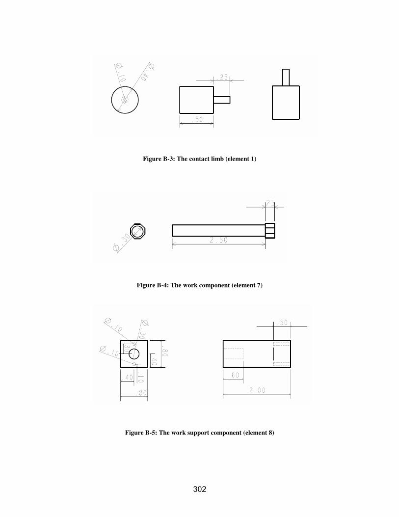
Figure B-3: The contact limb (element 1)

Figure B-4: The work component (element 7)

Figure B-5: The work support component (element 8)

#> #�

Figure B-6: The fulcrum component (element 9)

Figure B-7: The fulcrum support element (element 10)

#> &�

�� 7 � � � �� 4 � � � � ��,�7 � � � �� 4 � � � � ��,�7 � � � �� 4 � � � � ��,�7 � � � �� 4 � � � � ��, ��

#> *�

#> 9�

�� "�� "�� "�� "�� '8". �� 0� '�� !2�� '8". �� 0� '�� !2�� '8". �� 0� '�� !2�� '8". �� 0� '�� !2��

FR1 – Hold workpiece to the required accuracy FR1.1 – Locate the workpiece FR1.1.1 – Provide location directions FR1.1.1.1 – Provide location direction in y direction (0,1,0) FR1.1.1.2 – Provide location direction in x direction (1,0,0) FR1.1.1.3 – Provide location direction in z direction (0,0,1) FR1.1.1.4 – Provide location orientation around x axis (0,1,0) FR1.1.1.5 – Provide location orientation around y axis (1,0,0) FR1.1.1.6 – Provide location orientation around z axis (0,1,0) FR1.1.2 – Provide contact between locator and workpiece FR1.1.2.1 – Contact workpiece with locator P1 FR1.1.2.2 – Contact workpiece with locator T1 FR1.1.2.3 – Contact workpiece with locator S1 FR1.1.2.4 – Contact workpiece with locator P2 FR1.1.2.5 – Contact workpiece with locator S2 FR1.1.2.6 – Contact workpiece with locator P3 FR1.2 – Control accuracy of location FR1.2.1 – Locate workpiece to required drawing tolerances FR1.2.1.1 – Locate at location point P1 to an accuracy of xx.xx inches 0.0100 inches FR1.2.1.2 – Locate at location point T1 to an accuracy of xx.xx inches 0.0025 inches FR1.2.1.3 – Locate at location point S1 to an accuracy of xx.xx inches 0.0028 inches FR1.2.1.4 – Locate at location point P2 to an accuracy of xx.xx inches 0.0100 inches FR1.2.1.5 – Locate at location point S2 to an accuracy of xx.xx inches 0.0028 inches FR1.2.1.6 – Locate at location point P3 to an accuracy of xx.xx inches 0.0100 inches FR1.2.2 – Compensate for machine misalignment

FR1.2.2.1 – Compensate for machine misalignment of xx.xx inches in the y-direction 2E-005 inches

FR1.2.2.2 – Compensate for machine misalignment of xx.xx inches in the x-direction 2E-005 inches

FR1.2.2.3 – Compensate for machine misalignment of xx.xx inches in the z-direction 2E-005 inches

FR1.2.2.4 – Compensate for machine misalignment of xx.xx radians around the x-axis 8.7266E-005

FR1.2.2.5 – Compensate for machine misalignment of xx.xx radians around the y-axis 8.7266E-005

FR1.2.2.6 – Compensate for machine misalignment of xx.xx radians around the z-axis 8.7266E-005

FR1.2.3 – Compensate for casting variations at locator/workpiece interfaces

FR1.2.3.1 – Compensate for casting variations of xx.xx inches at locator P1/workpiece interface 0.002 inches

FR1.2.3.2 – Compensate for casting variations of xx.xx inches at 0.002 inches

#> :�

locator T1/workpiece interface

FR1.2.3.3 – Compensate for casting variations of xx.xx inches at locator S1/ workpiece interface 0.002 inches

FR1.2.3.4 – Compensate for casting variations of xx.xx inches at locator P2/ workpiece interface 0.002 inches

FR1.2.3.5 – Compensate for casting variations of xx.xx inches at locator S2/ workpiece interface 0.002 inches

FR1.2.3.6 – Compensate for casting variations of xx.xx inches at locator P3/ workpiece interface 0.002 inches

FR2 – Support workpiece against machining forces experienced during machining FR2.1 – Hold workpiece in situ during machining FR2.1.1 – Provide clamping in appropriate directions FR2.1.1.1 – Clamp w/piece against locator P1 with a force of xx lbs 50 lbs FR2.1.1.2 – Clamp w/piece against locator T1 with a force of xx lbs 50 lbs FR2.1.1.3 – Clamp w/piece against locator S1 with a force of xx lbs 50 lbs FR2.1.1.4 - Clamp w/piece against locator P2 with a force of xx lbs 50 lbs FR2.1.1.5 - Clamp w/piece against locator S2 with a force of xx lbs 50 lbs FR2.1.1.6 - Clamp w/piece against locator P3 with a force of xx lbs 50 lbs FR2.1.2 – Support the workpiece during machining FR2.1.2.1 – Ensure locator stiffness at locator P1 is xx lb/in 37417 lb/in FR2.1.2.2 – Ensure locator stiffness at locator T1 is xx lb/in 252543 lb/in FR2.1.2.3 – Ensure locator stiffness at locator S1 is xx lb/in 231810 lb/in FR2.1.2.4 – Ensure clamping stiffness at locator P1 is xx lb/in 29934 lb/in FR2.1.2.5 – Ensure clamping stiffness at locator T1 is xx lb/in 222971 lb/in FR2.1.2.6 – Ensure clamping stiffness at locator S1 is xx lb/in 204666 lb/in FR2.1.2.7 – Ensure locator stiffness at locator P2 is xx lb/in 37417 lb/in FR2.1.2.8 – Ensure locator stiffness at locator S2 is xx lb/in 231810 lb/in FR2.1.2.9 – Ensure clamping stiffness at locator P2 is xx lb/in 29934 lb/in FR2.1.2.10 – Ensure clamping stiffness at locator S2 is xx lb/in 204666 lb/in FR2.1.2.11 – Ensure locator stiffness at locator P3 is xx lb/in 37417 lb/in FR2.1.2.12 – Ensure clamping stiffness at locator P3 is xx lb/in 29934 lb/in FR2.1.3 – Provide clamping points FR2.1.3.1 – Contact workpiece with clamp CP1 FR2.1.3.2 – Contact workpiece with clamp CT1 FR2.1.3.3 – Contact workpiece with clamp CS1 FR2.1.3.4 - Contact workpiece woth clamp CP2 FR2.1.3.5 - Contact workpiece with clamp CS2 FR2.1.3.6 - Contact workpiece with clamp CP3 FR2.1.4 – Provide clamping points FR2.1.4.1 – Provide clamping orientation for clamp CP1 (0,-1,0) FR2.1.4.2 – Provide clamping orientation for clamp CT1 (-1,0,0) FR2.1.4.3 – Provide clamping orientation for clamp CS1 (0,0,-1) FR2.1.4.4 - Provide clamping orientation for clamp CP2 (0,-1,0)

#> <�

FR2.1.4.5 - Provide clamping orientation for clamp CS2 (-1,0,0) FR2.1.4.6 - Provide clamping orientation for clamp CP3 (0,-1,0)

DP1 Plane DP1.1 Plane_Var3 DP 1.1.1 – Locator/workpiece interface orientation DP 1.1.1.1 – Locator P1/workpiece interface orientation 2 DP 1.1.1.2 – Locator T1/workpiece interface orientation 16 DP 1.1.1.3 – Locator S1/workpiece interface orientation 3 DP 1.1.1.4 – Locator P2/workpiece interface orientation 2 DP 1.1.1.5 – Locator S2/workpiece interface orientation 3 DP 1.1.1.6 – Locator P3/workpiece interface orientation 1 DP 1.1.2 – Workpiece/locator interface contact positions DP 1.1.2.1 – Locator P1 position (6.75,1,0.25) DP 1.1.2.2 – Locator T1 position (0,2.5,2.5) DP 1.1.2.3 – Locator S1 position (0.25,2.25,0) DP 1.1.2.4 – Locator P2 position (3.639,1,4.75) DP 1.1.2.5 – Locator S2 position (5.75,2.25,0) DP 1.1.2.6 – Locator P3 position (0.25,0,0.25) DP 1.2 – Locator unit accuracy parameters DP 1.2.1 – Locator unit tolerances DP 1.2.1.1 - Vertical locating unit tolerance of xx.xx inches Unit ID DP 1.2.1.2 - Horizontal locating unit tolerance of xx.xx inches Unit ID DP 1.2.1.3 - Horizontal locating unit tolerance of xx.xx inches Unit ID DP 1.2.1.4 - Vertical locating unit tolerance of xx.xx inches Unit ID DP 1.2.1.5 - Horizontal locating unit tolerance of xx.xx inches Unit ID DP 1.2.1.6 - Vertical locating unit tolerance of xx.xx inches Unit ID DP 1.2.2 – Spacers between fixture base and machine table

DP 1.2.2.1 – Assignment of machine misalignment tolerance of xx.xx inches in the y-direction 2E-005 inches

DP 1.2.2.2 – Assignment of machine misalignment tolerance of xx.xx inches in the x-direction 2E-005 inches

DP 1.2.2.3 – Assignment of machine misalignment tolerance of xx.xx inches in the z-direction 2E-005 inches

DP 1.2.2.4 – Assignment of machine misalignment tolerance of xx.xx radians around the x axis

8.7266E-005 radians

DP 1.2.2.5 – Assignment of machine misalignment tolerance of xx.xx radians around the y axis

8.7266E-005 radians

DP 1.2.2.6 – Assignment of machine misalignment tolerance of xx.xx radians around the z axis

8.7266E-005 radians

DP 1.2.3 – Locator unit spacers at locator/workpiece interfaces

DP 1.2.3.1 – Assignment of surface tolerance of xx.xx inches at P1/workpiece interface 0.002 inches

DP1.2.3.2 – Assignment of surface tolerance of xx.xx inches at T1/workpiece interface 0.002 inches

#> =�

DP 1.2.3.3 – Assignment of surface tolerance of xx.xx inches at S1/workpiece interface 0.002 inches


DP 1.2.3.5 – Assignment of surface tolerance of xx.xx inches at S2/workpiece interface 0.002 inches


DP 2 – Fixture unit force capabilities DP 2.1 – Clamping unit force capabilities DP 2.1.1 – Clamping unit forces

DP 2.1.1.1 – Vertical clamp CP1 opposing workpiece/P1 interface with clamping force of xx lbs Unit ID

DP 2.1.1.2 – Horizontal clamp CT1 opposing workpiece/T1 interface with clamping force of xx lbs Unit ID

DP 2.1.1.3 – Horizontal clamp CS1 opposing workpiece/S1 interface with clamping force of xx lbs Unit ID


DP 2.1.1.5 - Horizontal clamp CS2 opposing workpiece/S2 interface with clamping force of xx lbs Unit ID


DP 2.1.2 – Unit stiffness DP 2.1.2.1 – Locator P1 stiffness of xx.xx lbs/in Unit ID DP 2.1.2.2 – Locator T1 stiffness of xx.xx lbs/in Unit ID DP 2.1.2.3 – Locator S1 stiffness of xx.xx lbs/in Unit ID DP 2.1.2.4 – Clamping unit CP1 stiffness of xx.xx lbs/in Unit ID DP 2.1.2.5 – Clamping unit CT1 stiffness of xx.xx lbs/in Unit ID DP 2.1.2.6 – Clamping unit CS1 stiffness of xx.xx lbs/in Unit ID DP 2.1.2.7 – Locator unit P2 stiffness of xx.xx lbs/in Unit ID DP 2.1.2.8 – Locator unit S2 stiffness of xx.xx lbs/in Unit ID DP 2.1.2.9 – Clamping unit CP2 stiffness of xx.xx lbs/in Unit ID DP 2.1.2.10 – Clamping unit CS2 stiffness of xx.xx lbs/in Unit ID DP 2.1.2.11 – Locator unit P3 stiffness of xx.xx lbs/in Unit ID DP 2.1.2.12 – Clamping unit CP3 stiffness of xx.xx lbs/in Unit ID DP 2.1.3 – Clamping points DP 2.1.3.1 – Clamp CP1 position (6.75,2.35,0.25) DP 2.1.3.2 – Clamp CT1 position (6,2.5,2.5) DP 2.1.3.3 – Clamp CS1position (0.25,2.25,5) DP 2.1.3.4 - Clamp CP2position (2,4.5,4.75) DP 2.1.3.5 - Clamp CS2 position (5.75,2.25,5) DP 2.1.3.6 - Clamp CP3position (0.25,5,0.25) DP 2.1.3 – Clamping points

DP 2.1.4.1 – Clamp CP1/workpiece interface orientation (workpiece surface) 5

#�> �

DP 2.1.4.2 – Clamp CT1/workpiece interface orientation (workpiece surface) 6

DP 2.1.4.3 – Clamp CS1/workpiece interface orientation (workpiece surface) 17

DP 2.1.4.4 - Clamp CP2/workpiece interface orientation (workpiece surface) 7

DP 2.1.4.5 - Clamp CS2/workpiece interface orientation (workpiece surface) 17

DP 2.1.4.6 - Clamp CP3/workpiece interface orientation (workpiece surface) 15

#��

�� 6�� 6�� 6�� 6� �� . � �� 3 � �� 6 �� . � �� 3 � �� 6 �� . � �� 3 � �� 6 �� . � �� 3 � �� 6 ��

��

Case Cost ($) Weight (lbs) Loading time (mins)

Assembly time (mins)

Unloading time (mins)

VL011C1 4.112 0.4 0 1.9 0 HL013C1 5.56 0.7 0 2.3 0

VC0132C1 1.799 1.172 0.5833 4.82 0.45 HC021C1 1.41 0.8 0.45 3.5 0.4 VC021C1 1.799 1.172 0.5833 4.82 0.45

Table E-1: Constraint attribute performance values for reference design solution

#�!�

�� "�� / � � � �� "�� / � � � �� "�� / � � � �� "�� / � � � ��

Figure F-1: Beam dimensions (elements 2, 3, 4, 5, 6)

Figure F-2: The contact limb (element 1)

Figure F-3: The work component (element 7)

#�#�

Figure F-4: The work support component (element 8)

Figure F-5: The fulcrum component (element 9)

Figure F-6: The fulcrum support element (element 10)

#�&�

�� 4 �� 4 �� 4 �� 4 ��7 � � � �� 7 � � � �� 7 � � � �� 7 � � � ��

#�*�

�� ; �� ; �� ; �� ; ��$� � �� $� � �� $� � �� $� � ��

#�9�

�� $� � �� $� � �� $� � �� $� � ��

Subject case: VC021C1 Element number: 1 Set diameter dimension to: 0.49678089 Modify connector length (mate_to connector) by: 0.048390445 Set 'mate to' connector diameter to: 0.124195223 Set 'mate to' connector hole diameter to: 0.124195223 Set connector offset (mate to) diameter to: 0 Element number: 2 Set start_b dimension to: 0.59678089

Dimension measured: Across local central

axis Set 'mate from' connector hole diameter to: 0.124195223 Modify connector hole (mates from) length by: 0.048390445 Set connector offset (mate from) diameter to: 0 Set end_b dimension to: 0.59678089


axis Set start_h dimension to: 0.69678089


axis Set end_h dimension to: 0.69678089


axis Element number: 3 Set start_b dimension to: 0.59678089


axis Set end_b dimension to: 0.59678089



#�:�




axis Element number: 4 Set start_b dimension to: 0.59678089








axis Set slot width to: 0.39678089 Element number: 5 Set start_b dimension to: 0.59678089








axis Set slot width to: 0.39678089 Element number: 6 Set start_b dimension to: 0.59678089

#�<�








axis Set slot width to: 0.39678089 Element number: 7 Set position to: 2.175 Position axis: Unit y positive Set length to: 1.675 Modify connector length by: 0.18428089 Set diameter dimension to: 0.39678089 Set 'mate to' connector diameter to: 0.39678089 Set 'mate to' connector hole diameter to: 0.39678089 Set connector offset (mate to) diameter to: 0 Element number: 8 Set length to: 2.175 Modify connector hole depth by: 0.0875 Connector hole depth measured from: 'Mating to' surface: Modify connector length by: 0.0875 Modify connector hole depth by: 0.0875 Connector hole depth measured from: 'Mating from' surface: Set start_b dimension to: 0.89678089


axis Set 'mate to' connector diameter to: 0.112097611 Set 'mate to' connector hole diameter to: 0.112097611

#�=�

Set connector offset (mate to) diameter to: 0.672585668 Set 'mate from' connector hole diameter to: 0.39678089 Set connector offset (mate from) diameter to: 0 Set end_b dimension to: 0.89678089






axis Element number: 9 Set position to: 2.175 Position axis: Unit y positive Set length to: 1.675 Modify connector hole depth by: 0.0875 Connector hole depth measured from: 'Mating to' surface: Modify connector length by: 0.175 Set diameter dimension to: 0.49678089 Set 'mate to' connector diameter to: 0.49678089 Set 'mate to' connector hole diameter to: 0.49678089 Set connector offset (mate to) diameter to: 0 Element number: 10 Set length to: 2.175 Modify connector hole depth by: 0.0875 Connector hole depth measured from: 'Mating to' surface: Modify connector length by: 0.0875 Modify connector hole depth by: 0.0875 Connector hole depth measured from: 'Mating from' surface: Set start_b dimension to: 0.89678089


axis

#!> �

Set 'mate to' connector diameter to: 0.112097611 Set 'mate to' connector hole diameter to: 0.112097611 Set connector offset (mate to) diameter to: 0.672585668 Set 'mate from' connector hole diameter to: 0.49678089 Set connector offset (mate from) diameter to: 0 Set end_b dimension to: 0.89678089






axis

CAFixD – A CASE-BASED REASONING METHOD FOR FIXTURE …

Documents

Transcript of CAFixD – A CASE-BASED REASONING METHOD FOR FIXTURE …