Chapter 1

Introduction

Modern computer systems are very important to our lives. Use spans fromspace shuttles and robots investigating foreign planets over critical hospitalsystems, power-plant control and computer systems controlling aeroplanes andcars, to home banking, e-mail, and word processing.

Some of the systems using computers can be considered highly critical, ei-ther because they are very expensive to produce, such as robots investigatingforeign planets, or because human lives depend on them, such as computerscontrolling aeroplanes and cars, and systems in hospitals and power-plants.These systems need to be correct, because their failure can cause loss of hu-man lives or enormous economical losses. Faulty computer software has beenthe cause of numerous disasters [81]. Disasters range from killing at least sixpeople due to radiation overdoses because the Therac-25 radiation therapy ma-chine [109] was unable to detect a human error and issue a warning, over eco-nomical losses, including the Ariane 5 lifting rocket [39], which self-destructedbecause a 64 bit floating point value was erroneously converted to a 16 bit inte-ger and the error handler, which was supposed to take care of errors when toolarge values were converted, had been disabled for efficiency reasons, causingthe computer to crash. The Mars Climate Orbiter [48] crashed while trying toland due to a mix-up between metric and U.S. customary units, causing the lossof the robot. NASA satellite software designed to measure holes in the ozonelayer [129] ignored values deviating from the expected values caused a hole inthe ozone layer to be ignored for eight years. These examples illustrate howerrors in computer software can lead to vast economical losses, environmentaldisasters, and loss of human lives, so for critical software it is worth the effortto ensure that the software has no errors.

The goal of this work is to contribute to the design and improvement ofmethods for avoiding such catastrophic computer malfunctions. This is done byconstructing a formal model of the system we wish to construct, validate thatthe formal model corresponds to the intended system using a domain-specificvisualisation, and formally verify that the formal model satisfies properties re-quired of the system, e.g., that it is impossible for a human error to cause thedeath of other humans. Correctness depends on the computers themselves, thehardware, and the programs they run, the software. Both are equally impor-tant and need to be correct in order for the entire system to be correct. In thisthesis we focus on the correctness of the software, not because the hardware isdeemed less important, but because we assume that somebody else takes careof the correctness of hardware.

In the rest of this chapter, we first describe what we consider formal modelsof computer systems. We then turn to describing how to verify the behaviour

3

4 Chapter 1. Introduction

of formal models and how to visualise that behaviour. After that we providedirections for arriving at a correct implementation from the formal model, andwe end this chapter by providing a guide to the rest of this thesis.

1.1 Approaches to Software Validation

One classical approach to program correctness is to annotate them with for-mal expressions, e.g., using Hoare logic [70], from which we can derive desiredcorrectness properties. We must manually or semi-automatically prove thatthe program indeed satisfies these annotations. This approach has a numberof disadvantages. Firstly, the approach requires that humans manually findthe correct annotations and prove their correctness. This is a lot of manualwork, which is very difficult for large systems. Secondly, the approach requiresthat whenever a change is made to the system, some expressions must be re-evaluated and re-proven, which makes changes expensive.

Given the limitation of classical approaches to correctness, we instead con-sider an approach based on construction of models. To illustrate this, we con-sider a parallel in the physical world, namely building a house. When a cus-tomer wants a new house, but is unable to build it himself, he hires some con-tractors to do it for him. The customer here corresponds to the customer whowants a computer program, and the contractors correspond to software com-panies or programmers. The customer can send requirements (such as size,number, and placement of rooms) to the contractors, who then build the houseaccording to their interpretation of these requirements. The requirements fromthe customer have a direct counterpart in the computer software, where we callsuch requirements a requirements specification or just specification for short.The specification may be more or less precise and state what is required of thecomputer program. This is illustrated in Fig. 1.1(a). Here we see the customer(upper left corner) write a specification (lower left corner), which is then inter-preted by the contractor (middle), who builds a house, (right), based on his in-terpretation of the specification. As we can see, the specification is ambiguous(what is “red” and how should the 180 m2 be distributed?) and incomplete (whatshould the roof look like?), which leads to multiple possible implementations.If the construction of the building has been outsourced to multiple contractors,they would probably interpret the specification in different ways, which couldlead to houses that could not even be assembled in the end (e.g., the roof of theinterpretation (I) is too small for (II) ). The same problems arise when dealingwith software. Ambiguities lead to software that does not do what the customerintended and different interpretations by different software companies or pro-grammers lead to components that cannot inter-operate. In Fig. 1.1(b), we seethat the customer thinks of a protocol which allows two computers to communi-cate in both directions over a wireless link, but the specification is ambiguous(what is “nodes”) and incomplete (it does not state that communication shouldbe bi-directional and over a wireless link), so the programmer, correspondingto the contractor in the house example, may implement the protocol under theassumption that two stationary computers communicate over a wired link (I)or as a media-server communicating uni-directionally with a computer over asatellite link (II).

In the real world, a contractor would not work directly from the specifica-tion provided by the customer. Instead, an architect would try to interpret therequirements from the customer and create a precise and complete represen-tation in the form of blueprints. This situation is depicted in Fig. 1.2. Nowthe contractor is certain of how the house should be constructed, and multi-

1.1. Approaches to Software Validation 5

*.

0.

2464

04

9..9

9..99

(a)

(b)

Figure 1.1: Construction directly from the specification.

*.

0.

2464

!%

♫

%

%

(a)

!"#$%&'$()*"+,(-.(#)

♫

!"#$%&'$"+(&

/#"0#%$$(#

!$&'

(

(

!$&'

!$**'

!$&'

!$&'!$&'

+,-

/2

/2+&

6+&

/2

+

&-,

>?@A

B&

+

&-,

>?@A

CD&EDFF,

!$*E/AG*'((!$*H--*'((!I$*JKKKKKK*'

>?@A

1$.&($(2)%)3"2

(b)

Figure 1.2: Construction using a formal model.

ple contractors can be hired to make the different parts of the house with-out problems. This approach is better than the previous one, as we have ob-tained a precise and complete description of the house we want to construct.We can use this approach for software construction as well. Here we call theblueprints a formal model of the program. We require that the formal modelis constructed in a formal language with a formal semantics, such as colouredPetri nets [91], state charts [65], message sequence charts [67] (a variant ofwhich is known as UML [131] sequence diagrams), Petri nets [138], CCS [123],PROMELA [77,154], ambient calculus [17], or π-calculus [124]. We will not al-low a formal model to be specified as a natural language specification or usingsemi-formal notations such as UML [131]. The formal model is constructed bya formal methods expert.

While the method in Fig. 1.2 ensures that we get a precise and completeformal description of what to construct, it does not ensure that the formalmodel corresponds to the customer’s intentions. We can see in Fig. 1.2 thatthe house/network protocol the customer is thinking of is different from theone constructed by the contractor/programmer. This is because the originalnatural-language specification was not accurate or because the architect mis-understood it. We would therefore like the customer to validate that the formaldescription (the blueprints or the formal model) of the system corresponds tohis intentions. Alas, the customer may not understand the blueprints or formalmodel. This may be stretching the parallel a little, as most people have someunderstanding of how to read blueprints, but it may not be easy to understandhow the living room will look in afternoon sunlight from a set of blueprints.In any case, the customer is seldom able to read a formal model of a software

6 Chapter 1. Introduction

*.

0.

2464

!%

%

!%!%%

(a)

.#")"4'*%2+&('&",,4'5'2"+(,

6

7.(

!"#$%&'$()*"+,(-.(#)

!"#$%&'$()*"+,(-.(#)

!$&'

(

(

!$&'

!$**'

!$&'

!$&'!$&'

+,-

/2

/2+&

6+&

/2

+

&-,

>?@A

B&

+

&-,

>?@A

CD&EDFF,

!$*E/AG*'((!$*H--*'((!I$*JKKKKKK*'

>?@A

(b)

Figure 1.3: Using visualisation to ensure the formal model corresponds to thecustomers intentions.

system, and this is the scenario we are really interested in.

To make the customer understand the model of the system, we assume thatthe architect/formal methods expert or somebody else, who understands theformal model, creates a visualisation of the model. In the house example, athree dimensional physical model of the house may be constructed. It is placedin a physical model of the surroundings, which allows the customer to look atthe model and see if it fits with his ideas. He may even experiment with it, e.g.,by moving a lamp around it simulating how the sun looks at different times ofthe day. This visualisation may cause the customer to improve the specifica-tion by making requirements more precise and by specifying things missing inthe original specification. In the physical world, the blueprints would then beupdated and a new visualisation would be created. This is shown in Fig. 1.3(a).In the software world, we would create a visualisation of the software we areabout to write, corresponding, e.g., to a prototype [44], and let the user ex-periment with the prototype, thereby improving the specification. Often theprototype runs as a computer program, as shown in Fig. 1.3(b).

By the method in Fig. 1.3, we can construct a complete formal model ofthe system we want to construct. The idea is to use this formal specification tocheck properties of the system we want to eventually construct. In the physicalworld we may want to check that the house abides by the legislation (e.g. itmay be illegal to construct red houses in a certain neighbourhood), and thatit is physically possible to construct the house (e.g. that the roof is not tooheavy). This can be done as outlined in Fig. 1.4. Here we assume a blueprintor a formal model—which may or may not correspond to some real system—and some requirements. In the physical world an engineer would look at therequirements and the blueprints together, and either arrive at the conclusionthat the blueprints satisfies the requirements, or find some errors, which arethen fixed in the blueprints, e.g., by requiring that the walls of the house ismade of more solid material. In the software world, we assume that the formalmodel and the requirements are on some form we can use as input to a verifier.The verifier can give two answers, either the requirements hold or they donot. If the requirements hold, we are satisfied with an “Ok” from the verifier,whereas we would like an error report if the requirements are not satisfiedby the model. We can use this error report as input for further refinementof the model and the requirements. Sometimes the error is really an error inthe model, either because we have incorrectly modelled the requirements (for

1.2. Behavioural Models of Concurrent Systems 7

(a)

;<=>

?>

@

!$&'

(

(

!$&'

!$**'

!$&'

!$&'!$&'

+,-

/2

/2+&

6+&

/2

+

&-,

>?@A

B&

+

&-,

>?@A

CD&EDFF,

!$*E/AG*'((!$*H--*'((!I$*JKKKKKK*'

>?@A

(b)

Figure 1.4: Verification of formal models.

example if the requirements specifies sufficiently strong walls but the modelincorrectly specifies the strength as too low) or because the requirements areincorrect (for example if the requirements specify that walls should be too thin,so they are not able to carry the roof). In that case, we need to change the modeland/or the requirements. Sometimes the error is an erroneous requirement,e.g., a too strict requirement (for example houses may be allowed to be red,just not crimson). Whenever we fix an error in the formal model, we also fixan error in the product, assuming that the product is constructed exactly asdescribed by the formal model.

1.2 Behavioural Models of Concurrent Systems

Until now, we have talked about formal models of computer systems withoutdefining what we mean by that. In the physical world a model of the product,e.g., a house, is an abstract representation of the product, and we want a for-mal model of a computer system to also be an abstract representation of theproduct, i.e., the implementation. The advantage of a more abstract represen-tation is manifold. Firstly, it is often cheaper to construct an abstract model,as we do not have to deal with a lot of details, just like it is easier to draw astraight line and say it represents a wall of concrete than actually building thewall. Secondly, a more abstract representation usually has simpler behaviour,which makes analysis tractable for more complex systems.

In the rest of this thesis we solely focus on models of the behaviour of con-current systems [138], i.e., systems where computation is performed in multi-ple components or threads. Examples span from multi-threaded applicationsrunning on a single computer, such as a word processor which is able to con-tinue working while sending a document to the printer, to complex distributedalgorithms, such as network protocols which requires the cooperation betweenmultiple computers connected via a network to provide a service, such as trans-mitting packets safely over a faulty network. We consider concurrent systemsrather than single-threaded programs as the behaviour of concurrent systemsis much more complex. Correct behaviour of single-threaded systems can usu-ally be verified using, e.g., unit-testing [5], whereas concurrent systems notonly depend on the input to the program, but also on the timing of each com-ponent relative to the other components, which makes is difficult to write teststhat, in a reproducible way, exercise all possible interleavings of the compo-nents in question.

8 Chapter 1. Introduction

So, what is an abstract representation of a concurrent system? Supposewe are to create a network protocol for transmitting packets over an unreli-able network. If we were to actually implement the protocol, we would needto worry about receiving actual data from the network, which is operatingsystem-specific, we would need to decode binary data in order to put it into aform where we can process it, and we would need to set up equipment to actu-ally test our implementation. These implementation details and many otherslike them make the implementation complex and may hide the real applicationlogic. A model of a network protocol may disregard all of these implementationdetails, and can therefore focus on what we are actually interested in, namelythe behaviour of the protocol. A real prototype or implementation would alsosuffer from the fact that some actions happen very rarely in reality, but whenthey happen the correctness of the system can be affected. As an example,packet losses happen rarely in real settings, but depending at which point theyhappen during the execution of a network protocol, they can have catastrophicconsequences. A model of the system can be controlled, and we can intention-ally drive the model into rarely occurring situations to observe the behaviourof the system in such situations.

To describe our models, we need a modelling language. Most of the workdescribed in this thesis has been developed in the context of coloured Petrinets [91], but is independent of the formalism, and could have been created us-ing many other formal modelling languages. A coloured Petri net is a labelleddirected bipartite graph. In Fig. 1.5(a) we see a simple model of a networkprotocol, created in CPN Tools [C1,33], a tool for modelling with coloured Petrinets. The model is the same as the one used in [T3] (except for typograph-ical changes), which is a simplified version of a network protocol introducedin [91]. The nodes of a coloured Petri net are called places and transitions,and are drawn as ellipses and rectangles, respectively. The model in Fig. 1.5(a)has six places, Out Buffer, Send ID, Network 1, In Buffer, Receive ID, and Net-work 2, and four transitions, Send Data, Drop, Receive Data, and Receive Ack.Places have an associated type and can contain a multi-set of tokens of thattype. For example, in Fig. 1.5(a), the place Out Buffer has type PACKET andcontains two tokens. The number of tokens is written inside the circle next tothe place and the values of the tokens are written inside the rectangle nearby.On the place Out Buffer, each token is a pair of a packet sequence number andthe packet contents (i.e., of type PACKET). We see that a packet numbered 1containing ”Formal” is scheduled to be transmitted as is packet number 2 withdata ” model”. A transition is enabled if there exist an assignment of values toall variables around it so that all the tokens required by arc expressions, withthe proper values inserted, are available on input places (places connected toa transition via an arc from the place to the transition). As an example, pack-ets are transmitted by the Send Data. This transition is enabled in Fig. 1.5(a)if we assign the value 1 to id and ”Formal” to data. We write Send Data{id =1, data = ”Formal”} to represent the transition Send Data with this binding ofits variables. In Fig. 1.5(a) we have indicated that Send Data{id = 1, data =”Formal”} is enabled by a green highlighting of the transition Send Data. If atransition is enabled it can be executed and the result is that tokens are re-moved from input places according to the arc expressions and new tokens areproduced on output places (places connected to the transition via an arc fromthe transition to the place) according to the arc expressions. A double arc isjust an abbreviation for an arc in each direction with the same expression. Theresult of executing Send Data{id = 1, data=”Formal”} in Fig. 1.5(a) is shown inFig. 1.5(b). Here a new packet is produced on the place Network 1, correspond-ing to transmitting a packet onto the network. The packet is not removed from

1.2. Behavioural Models of Concurrent Systems 9

packets

packets^^[(id, data)]

id

idid+1

id+1

id

(id, data)

(id, data)

ReceiveAck

ReceiveData

SendData

[]

PACKETS

SendID

1

ID

Network 2

PACKET

1

ID

Network 1

PACKET

1`(1, "Formal")++1`(2, " model")

OutBuffer

PACKET

(id, "")

(id, data)

InBuffer

ReceiveID

Drop

(id, data)

(id, data)

1 1`1

2

1`(1,"Formal")++1`(2," model")

1

1`[]1 1`1

(a) Before executing Send Data{id = 1, data = ”Formal”}.

packets

packets^^[(id, data)]

id

idid+1

id+1

id

(id, data)

(id, data)

ReceiveAck

ReceiveData

SendData

[]

PACKETS

SendID

1

ID

Network 2

PACKET

1

ID

Network 1

PACKET

1`(1, "Formal")++1`(2, " model")

OutBuffer

PACKET

(id, "")

(id, data)

InBuffer

ReceiveID

Drop

(id, data)

(id, data)

1 1`1

1 1`(1,"Formal")

2

1`(1,"Formal")++1`(2," model")

1

1`[]1 1`1

(b) After executing Send Data{id = 1, data = ”Formal”}.

Figure 1.5: A formal model of a simple protocol able to transmit packets over anetwork which may drop packets.

the Out Buffer, so it can later be retransmitted if needed. The newly producedpacket can be dropped (Drop{id = 1, data = ”Formal”}) or successfully received(Receive Data{id = 1, data = ”Formal”, packets = []}). When packets are received,the counter on Receive ID is incremented by one, the packet is saved in the InBuffer, and an acknowledgement is sent back to the sender, so it knows that thepacket is successfully transmitted. Receive Ack receives such an acknowledge-ment, increments the counter in Send ID, so the sender can start transmittingthe next packet. We see that this models a simple network protocol, which isable to transmit packets over a network that may drop packets. The detailsof how the network works have been abstracted away and packets are repre-sented in an abstract way, so we do not have to perform complex translationsof binary data, which would hide the application logic.

10 Chapter 1. Introduction

1.3 Verification of Formal Models

Now we focus on the verifier in Fig. 1.4. Considering the house example, theverifier would be an engineer using techniques based on the laws of physics toverify properties of the house. Naturally, we would like a way to do that in thesoftware world as well.

In order to verify whether a formal model satisfies one or more properties,we use an analysis method. Basically, analysis methods fall into two categories:static analysis and dynamic analysis. Static analysis only looks at the descrip-tion of the model whereas dynamic analysis also looks at the behaviour of themodel. In the case of analysis of the network protocol described in the previ-ous section, static analysis would only look at the model in Fig. 1.5, whereasdynamic analysis would also look at the behaviour of the model. In this Sect.we will first look at static analysis and then turn to dynamic analysis.

1.3.1 Static Analysis

Static analysis is well-known from compilers. Compilers perform static anal-ysis to generate more efficient programs and to check for errors that may oc-cur in programs. Static analysis is performed when the program is compiles,whereas dynamic analysis as described in the next section is performed onrun-time. As an example, the Java language specification [62] cites that localvariables should be definitely assigned1 a value before they are used [62, Chap.16]. In both methods in Fig. 1.6, we are interested in checking whether thevariable y is definitely assigned a value before it is read. The variable is as-signed a value in lines 4 and 11 and read in lines 5 and 12. The only differencebetween the two problems is that the assignment in line 10 is dependent onthe evaluation of the boolean expression x == x. Thus, the method definitelyAs-signed from Fig. 1.6 is allowed whereas subtlyAssigned is not, even though thecondition of the if statement in line 10 would always be true. The propertywe actually want to check is that all variables have been assigned before theyare read, but it is impossible to check this property, so we instead check thesimpler property that all variables must definitely be assigned, thereby dis-carding subtlyAssigned even though it actually satisfies the desired property.Rice’s theorem [146] states that any non-trivial property of the behaviour ofprograms cannot be checked automatically. Here trivial properties are proper-ties that either hold for all programs or for no programs at all. Due to this prop-erty we have to translate properties stating something about the behaviour ofprograms into stronger properties stating something about the program. Thisis the strongest caveat of static analysis, as it is not always possible to find astronger requirement that does not discard important programs.

Hoare logic [70] is a classical technique for more advanced static analy-sis. The idea of Hoare logic is to annotate each statement of a program withpre- and post-conditions. Pre-conditions of one statement must follow logicallyfrom the post-condition of the previous statement. Proof rules for each kindof statement makes is possible to prove post-conditions from pre-conditions.Hoare logic makes it possible to state and prove properties, such as correct-ness of algorithms. The main difficulty of using Hoare logic is that sufficientlystrong pre-conditions must be chosen manually in order to prove the desiredpost-conditions.

1The specification of course defines this more precisely. The gist of the definition is that on alltraces, i.e., where both the then and else cases of an if-statement are considered, all variables mustbe assigned before they are read.

1.3. Verification of Formal Models 11

1 public class Assignments {2 public int definitelyAssigned(int x) {3 int y;4 y = x * 2;5 return y;6 }7

8 public int subtlyAssigned(int x) {9 int y;

10 if (x == x)11 y = x * 2;12 return y;13 }14 }

Figure 1.6: Two Java methods. One is accepted by the compiler while the otheris not. Neither contain any errors.

While Hoare logic requires ingenuity to come up with the correct pre- andpost-conditions, a simpler variant, namely types, have become so common mostprogrammers use them without ever really thinking about them. Types of vari-ables are statements that the values assigned to a variable always belong to acertain type. Consider again the methods in Fig. 1.6. How do we know that thestatement y = x * 2 always makes sense? What if x contains the string value”horse”? ”horse” * 2 certainly makes no sense. We know that the statementalways make sense, because we have declared that the parameter x must be oftype int, i.e., that it must always contain integers. Thus, whenever we use x,we know that we use an integer, so x * 2 is always successful, as multiplicationis defined on integers. In addition to requiring properties of our parameter, wealso promise that we always return an integer from both methods. We knowthat this is true, because the only value returned from either method is y (lines5 and 12), and we have declared that y is of type integer, which this is checkedwhenever we assign values to y, such as in y = x * 2. The type system alsoprevents us from making errors like calling definitelyAssigned(”horse”). In Javawe must explicitly state the types of variables, but it is also possible to makea strongly typed programming language even without this requirement, suchas Standard ML (SML) [159] or OCaml [108]. Instead of requiring the userto explicitly state the types of all variables, they can be automatically inferredfrom how the variables are used and consistency of the use is checked.

Type systems can also be used to check properties of certain modelling lan-guages, e.g., the ambient calculus [17]. The ambient calculus consists of am-bients, which are located inside each other. Ambients can move in and outof each other, dissolve neighbour ambients, and communicate with neighbourambients. A problem of the ambient calculus is that it is possible to send bothambients and operations over channels. This means that we may arrive at asituation where we receive an ambient on a channel and try to execute it, as-suming it is a operation, or we receive an operation and try to move inside it.Such nonsense uses of channels can be avoided if we are careful, but we canalso devise a type system which checks that do not make such errors. In [15]Cardelli et al. devise three type systems for the ambient calculus, among those,one which checks that nonsense use of data received over channels does nothappen. Another type system from [15] checks whether it is possible for am-

12 Chapter 1. Introduction

bients with a certain name to dissolve ambients with another name (whichcan be bad if, e.g., it is possible to send two packets to a remote computer andone packet contains code which is able to open the other packet to unveil avirus). The full result of [15] is a type system, which, in addition to checking heaforementioned two properties, also checks whether ambients with a certainname are able to enter ambients with another name, which can, e.g., be usedto check the effectiveness of firewalls (if malicious code is able to enter throughthe firewall it is not effective). Ambients need not be explicitly typed, muchlike how values do not need to be typed in SML, but any process that can becorrectly typed exhibit the desired behaviour at run-time. Type systems needto be developed and proved correct for each kind of property we would like tocheck, and are therefore not that applicable for proving arbitrary properties,but useful for guaranteeing absence of a certain kind of errors. Furthermore,type systems are useful when translating from one formalism to another usinga translation inductive in the structure of the source formalism. By explicitlyassigning types to the result of the translation, we can inductively prove ab-sence of a certain kind of errors (the kind guaranteed by the type system) in alltranslated models.

Type systems are a special case of invariants. Invariants are properties thatmust always hold during the entire execution of a program or formal model.Type systems are invariants stating that a given variable always contains avalue from a given set or that something sent over a given channel is alwaysa channel, and Hoare logic uses invariants in loops. Of particular interestare invariants that can proven solely by looking at the program or the for-mal model. Coloured Petri nets also allow the specification of invariants—infact two dual kinds of invariants: transition invariants and place invariants.Transition invariants state that the effect of executing a certain multi-set oftransitions (provided there are enough tokens initially) is the same as execut-ing no transitions at all. In Fig. 1.5(a) the effect of executing the transitionSend Data{id = 1, data = ”Formal”} is adding one token to Network 1 and theeffect of Drop{id = 1, data = ”Formal”} is the exact opposite. Thus we have atransition invariant 1‘Send Data{id = 1, data = ”Formal”} ++ 1‘Drop{id = 1, data= ”Formal”} (using the multi-set notation of CPN Tools). A place invariant isa set of weight-functions, which, when applied to the tokens available on allplaces, always yields the same value. In Fig. 1.5(a), if we map any integer to1‘0 on Send ID and Receive ID and all multi-sets of tokens on other places intothe empty multi-set, we get an invariant, as this always yields 2‘0. The weightfunctions should be linear in the number of tokens, and can map into any do-main desired. Invariants of CP-nets are not really that useful for analysis,as they must be interpreted manually depending on the model. Furthermore,calculating invariants requires calculation of inverse functions of the functionsappearing in the arc-expressions, which is not possible for CP-nets as the func-tions appearing in the arc-expressions can be arbitrary, making the calculationof invariants uncomputable. Work on automatically checking invariants forCP-nets has been implemented and shown to work on a small set of exam-ples by Toksvig in [158]. Invariants are more interesting for a simpler kindof Petri nets, namely Place-transition Petri nets (PT-nets) [36]. PT-nets can beconsidered as a simplified version of coloured Petri nets, but actually predatescoloured Petri nets. PT-nets are like coloured Petri nets except that all tokensare equal—the type of all places must be UNIT = {•} (written () for technicalreasons) and all arc expressions must be integers, signifying how many tokensare moved from each place. A PT-net version of the network protocol fromFig. 1.5 is shown in Fig. 1.7. The protocol in Fig. 1.7 is only able to transmita single packet, but otherwise behave like the coloured Petri net version. All

1.3. Verification of Formal Models 13

1`()

1`()

1`()

1`()

1`()

ReceiveAck

ReceiveData

SendData

UNIT

SendID

()

UNIT

Network 2

UNIT

()

UNIT

Network 1

UNIT

()

OutBuffer

UNIT

1`()

1`()

InBuffer

ReceiveID

Drop

1`()

1`()

1`()1

1

1

Figure 1.7: A simplified version of the network protocol from Fig. 1.7 createdas a PT-net.

places now have type UNIT and the values of the tokens have been removed.As no variables exist on any arcs, we no longer have to specify the variableswhen discussing enabling. The transition invariant 1‘Send Data ++ 1‘Drop ispreserved. The advantage of considering PT-nets when calculating invariantsis that we only need to compute the inverse of linear functions on integers,which is computable.

As mentioned, due to Rice’s theorem, it is not possible to answer questionsabout a model’s behaviour (at least models described using a Turing Com-plete [11] modelling language such as CP-nets) or a programs execution byonly looking at the model or program itself. For debugging it is not a prob-lem that we are unable to give exact answers, as we are often satisfied withbeing told about potential errors or proving absence of simple errors, explain-ing the success of static analysis, which gives a sound answer, meaning thatif the analysis states that no error exists, then no error exists (of the kind wecheck). Static analysis is not complete, though, so if static analysis discoversa problem, this does not necessarily mean that there really is an error. Someproperties are very difficult to determine using static analysis at a level finegrained enough to be really useful, however. Such properties include whetherallocated memory is always freed exactly once, and whether buffers can over-or under-flow. When we want to ensure that some run-time property holds, anapproximate answer may not be enough. The idea of dynamic analysis methodsis to explore the behaviour of the system during run-time.

1.3.2 Dynamic Analysis

The simplest way to check the run-time (dynamic) behaviour of a system is totest it, i.e., execute the system a number of times and manually or automati-cally check that the behaviour corresponds to the desired behaviour. Tests canbe written manually or created automatically [45] by a computer tool. Whendealing with models, we usually refer to the execution of the model as a simu-lation of the model. Tests makes it possible to unveil errors that are difficultto find with static analysis, but do not ensure absence of errors. In order toensure absence of errors, we need to ensure that our tests cover all possibleexecution paths. In order to do that, we build a reachability graph (also knownas a state space). A reachability graph is a directed labelled graph, where the

14 Chapter 1. Introduction

packets

packets^^[(id, data)]

id

idid+1

(id, data)

(id, "")

id+1

id

(id, data)

(id, data)

(id, data)

(id, data)

ReceiveAck

ReceiveData

Drop

SendData

InBuffer

[]

PACKETS

SendID

1

ID

Network 2

PACKET

ReceiveID

1

ID

Network 1

PACKET

OutBuffer

1`(1, "Formal")++1`(2, " model")

PACKET

Limit

UNIT()

()

()

2`()11`[]

1 1`11 1`1

21`(1,"Formal")++1`(2," model")

2

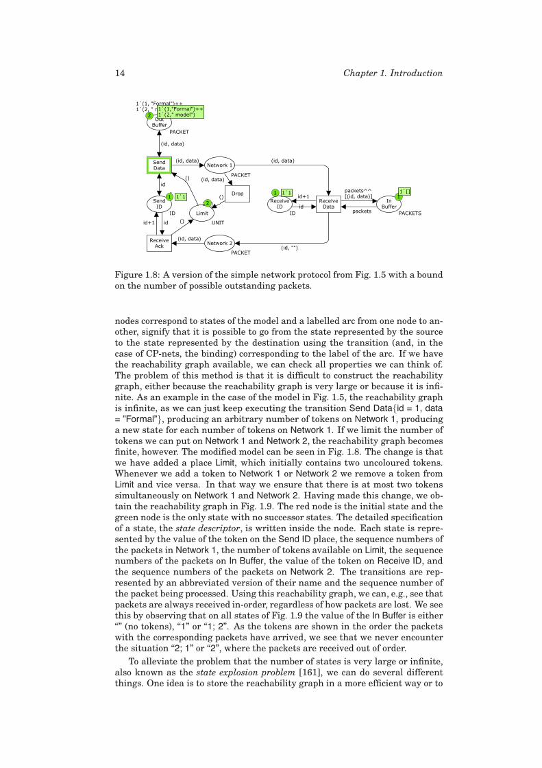
Figure 1.8: A version of the simple network protocol from Fig. 1.5 with a boundon the number of possible outstanding packets.

nodes correspond to states of the model and a labelled arc from one node to an-other, signify that it is possible to go from the state represented by the sourceto the state represented by the destination using the transition (and, in thecase of CP-nets, the binding) corresponding to the label of the arc. If we havethe reachability graph available, we can check all properties we can think of.The problem of this method is that it is difficult to construct the reachabilitygraph, either because the reachability graph is very large or because it is infi-nite. As an example in the case of the model in Fig. 1.5, the reachability graphis infinite, as we can just keep executing the transition Send Data{id = 1, data= ”Formal”}, producing an arbitrary number of tokens on Network 1, producinga new state for each number of tokens on Network 1. If we limit the number oftokens we can put on Network 1 and Network 2, the reachability graph becomesfinite, however. The modified model can be seen in Fig. 1.8. The change is thatwe have added a place Limit, which initially contains two uncoloured tokens.Whenever we add a token to Network 1 or Network 2 we remove a token fromLimit and vice versa. In that way we ensure that there is at most two tokenssimultaneously on Network 1 and Network 2. Having made this change, we ob-tain the reachability graph in Fig. 1.9. The red node is the initial state and thegreen node is the only state with no successor states. The detailed specificationof a state, the state descriptor, is written inside the node. Each state is repre-sented by the value of the token on the Send ID place, the sequence numbers ofthe packets in Network 1, the number of tokens available on Limit, the sequencenumbers of the packets on In Buffer, the value of the token on Receive ID, andthe sequence numbers of the packets on Network 2. The transitions are rep-resented by an abbreviated version of their name and the sequence number ofthe packet being processed. Using this reachability graph, we can, e.g., see thatpackets are always received in-order, regardless of how packets are lost. We seethis by observing that on all states of Fig. 1.9 the value of the In Buffer is either“” (no tokens), “1” or “1; 2”. As the tokens are shown in the order the packetswith the corresponding packets have arrived, we see that we never encounterthe situation “2; 1” or “2”, where the packets are received out of order.

To alleviate the problem that the number of states is very large or infinite,also known as the state explosion problem [161], we can do several differentthings. One idea is to store the reachability graph in a more efficient way or to

1.4. Behavioural Visualisation of Formal Models 15

Figure 1.9: The reachability graph of the simple network protocol in Fig. 1.8.

only store enough information that we are later able to reconstruct the reach-ability graph. Construction of the reachability graph can be done in two ways,either explicitly or symbolically. Explicit reachability graph analysis explic-itly store the reachability graph in memory, whereas symbolical reachabilitygraph analysis only has an implicit representation, e.g., by representing allstates as a logical formula satisfied by exactly the reachable states. For ex-plicit reachability graph analysis, we often use a reduction technique in orderto only require as much internal memory as is available. Examples of reduc-tion techniques are the sweep-line method [T1,25,104], which uses a notion ofprogress in the model to delete states that cannot be reached again, hash com-paction [155, 172], which does not store an actual representation of the statedescriptors, but only a hash value calculated from the state descriptor, calleda compressed state descriptor, and the ComBack method [T2], which is an ex-tension of hash compaction solving the problem of hash collisions, which arisewhen two state descriptors have the same hash value, meaning only successorsof one of the states is considered; by maintaining a spanning tree of the reach-ability graph, it is possible to reconstruct the full state descriptors and resolvehash collisions. Symbolic reachability graph analysis typically use, e.g., binarydecision diagrams [12] or multi-valued decision diagrams [96] to store statesefficiently.

Another approach is to only guarantee properties on traces of some finitelength. This is known as bounded model checking [8], and relies on tools thatare able to solve the SAT problem [148] for propositional logic, i.e., whetherthere exists an assignment to all propositional variables of a given proposi-tional formula, such that the formula evaluates to true. Bounded model check-ing is also an instance of symbolic model checking, where states are repre-sented using boolean formulae.

Another idea is to create a coverability graph [52, 97] instead of a reacha-bility graph. This method is specific to Petri nets, but the coverability graphis always finite and allows us to check certain interesting properties, e.g., tofind maximum number of tokens on all places. We get into more detail aboutreduction techniques in Chapter 2.

1.4 Behavioural Visualisation of Formal Models

When we have created a formal model of a concurrent system like the networkprotocol in Fig. 1.5, we would like to make sure that the constructed model

16 Chapter 1. Introduction

Figure 1.10: The Model-View-Controller design pattern.

corresponds to the intended system using the approach in Fig. 1.3. To intro-duce visualisations of formal models, we will first introduce the Model-View-Controller (MVC) [100] design pattern [54], which is the foundation for manyapproaches to visualisation of formal models.

1.4.1 The Model-View-Controller Design Pattern

A design pattern [54] is a recipe for how to do a certain task in a programminglanguage. The Model-View-Controller (MVC) [100] design pattern is a recipeon how to create graphical user interfaces that are able to manipulate a datastructure within the computer. The data structure may represent, e.g., a textdocument or the organisation of a company. When using the MVC design pat-tern, the data structure we wish to manipulate is called the model (not to beconfused with formal models as discussed previously). The user interface theuser see is called the view, and the code able to cause changes to the modelis called the controller. In Fig. 1.10 we see how the three parts of the systeminteract. When a user wishes to create a change in the model, an action in theuser interface, i.e., the view, is triggered. An example of this is when a buttonis clicked or an item is selected from a menu. This causes the view to invokethe corresponding function in the controller. The controller then changes themodel accordingly, e.g., removes a line of text or promotes a salesman to man-ager. When the model is changed, it alerts the view, which observes the modeland updates itself accordingly. This gives the user the impression that the de-sired update was performed in the user interface and that work is done on thegraphical view of the model rather than on the underlying model itself.

One important consequence of using the MVC design pattern is that it ispossible to have more than one view for each model. When a change is madein one view, all other views are updated as well. This happens because themodel alerts all views whenever a change occurs. As an example, consider theinteraction depicted in Fig. 1.11. Here two views, View 1 and View 2, are asso-ciated with a single model. The figure shows that a user initiates an action inView 1. This causes the view to invoke the corresponding code in the controller.The controller then changes the model accordingly. The model then alerts bothviews, which causes them to observe the model anew. Depending on the imple-mentation, the model may alert all views before any of them update themselvesaccording to the model, or each alert may be immediately followed by an up-date. In Fig. 1.11 we assume that all alerts happen before any observations.The views can show the same or they can show different aspects of the model.

1.4. Behavioural Visualisation of Formal Models 17

Figure 1.11: How two views associated with the same model are updated.

Figure 1.12: Screen-shot from the Eclipse Java editor.

Consider the screen-shot from Eclipse [41] in Fig. 1.12. Eclipse is a tool forediting Java programs. Here we see five different views on the class Place froma coloured Petri nets editor. At the upper right we see the actual code of theclass, and at the lower right we only see the embedded documentation of theconstructor of the class. At the lower left we see an overview of the class, andat the upper left we see a partial overview of the class hierarchy including theclass Place. Finally, we can see a tool-tip near the mouse in the middle of theimage, which shows an abbreviated version of the documentation for the itemunder the mouse. All of these views are different views of the same model andwe see that they show different details about the model. Some show (nearly)all details and some show very limited details about the model, but whenevera change is made to one of the views, e.g., if the class is modified in the upperright window, all the views are updated automatically.

We now let the formal model be the model of the MVC design pattern andwe let the visualisation be the view. The controller is usually the tool used tosimulate the formal model, but may also be integrated with the visualisation.

18 Chapter 1. Introduction

1.4.2 Behavioural Visualisation of Formal Models Usingthe Model-View-Controller Design Pattern

If the concurrent system we wish to develop and thus model and visualise isa simple form-filling application, such as a business intelligence or inventoryapplication, a visualisation can quite easily be constructed using the idea of aprototype [44]. A prototype is a simple implementation of a program in whichonly limited functionality has been implemented, but otherwise the prototypelooks and behaves as the real implementation. In MVC terms we implementonly the view and very simplistic models and controllers. Prototypes are valu-able as a tool for testing a user-interface before a costly construction of thereal product. The idea is that it is very easy and cheap to create a reason-ably professional-looking user interface using a GUI-builder, such as BorlandJBuilder [90] or Microsoft Visual Studio [167]. Normally, we would then ex-tend the purely visual prototype with simple code that make the prototype actas expected of the real program. If we, instead of a simplistic implementationof the model and controller, use a formal model in place of the model and thesimulation tool as controller, we get a product whose behaviour is defined by aformal model. As the GUI is a view of the formal model, it is possible to seethe state of the formal model. Whenever the formal model’s state is updated,the GUI is updated accordingly. By letting actions performed in the GUI corre-spond to actions in the formal model, it is also possible to stimulate the formalmodel, and it is thus possible to see and stimulate the execution of the formalmodel using a standard GUI.

Some times the model is not modelling a simple form-filling application,however. As an example, the network protocol from Sect. 1.2 is a more complexsystem. It is not obvious how we should create a user-interface that allows usto observe the behaviour of the system as a network protocol would not havea graphical user-interface except for configuration purposes. We could, how-ever, create a visualisation rooted in the network diagrams used to diagramthe layout of a large network, where all machines are drawn as icons and pack-ets as coloured dots like the one in Fig. 1.13. The figure shows the sender tothe left and the receiver to the right. The cloud represents the network. Thecoloured dots represent packets; green packets contain data en route from thesender to the receiver while red dots correspond to acknowledgements en routein the other direction. The number in the dots shows the sequence number ofthe packet. Below the sender and receiver, we see counters, representing thecounters on Send ID respectively Receive ID. Currently both of these are 1. Wemay be able to transmit packets by clicking on the sender. The graphics inFig. 1.13 is updated while packets are transmitted, e.g., to show whether pack-ets are dropped or successfully received as well as to show the current valuesof the counters. If we implement code which is able to show and maintain avisualisation like the one in Fig. 1.13, we can use it as view, the formal modelas model and the simulation tool as controller as in the case of the GUI appli-cation. This is an example of a domain specific visualisation, as we have useda visualisation that is likely to be familiar to the domain expert.

In this manner we can implement a model-based prototype, which has sev-eral advantages over a normal prototype or an implementation. As an example,it is possible to abstract away certain implementation details. In the case of thenetwork protocol, we are able to ignore any operating system-specific networkaccess and encoding/decoding of binary data. Compared to creating a proto-type written entirely in, e.g., Java we also obtain a formal specification of thesystem we wish to implement without representing the dynamics of the pro-tocol twice, once in the prototype and once in the formal model. The formal

1.5. Relationship between Formal Model and Implementation 19

Figure 1.13: Visualisation of a simple network protocol.

(a)

!$&'

(

(

!$&'

!$**'

!$&'

!$&'!$&'

+,-

/2

/2+&

6+&

/2

+

&-,

>?@A

B&

+

&-,

>?@A

CD&EDFF,

!$*E/AG*'((!$*H--*'((!I$*JKKKKKK*'

>?@A

(b)

Figure 1.14: Manual construction.

model can be used for analysis or as basis for an implementation as discussedin the next section. The use of a domain specific graphical user interface (thevisualisation) has the advantage that the design can be experimented with andexplored without having knowledge of the formal modelling language.

1.5 Relationship between Formal Modeland Implementation

Once we have constructed a formal model, we validate that it reflects the sys-tem we want to construct using the approach shown in Fig. 1.3 and describedin Sect. 1.4. Then, we verify that the model satisfies the requirements we mayhave using the method shown in Fig. 1.4 and described in Sect. 1.3. The nextstep is then to actually implement the system. In this section we look at fourways to arrive at an implementation based on a formal model.

The most straightforward way to obtain an implementation correspondingto a formal model is to look at the formal model and the specification and man-ually create the implementation, relying on experience to make a reasonabletranslation. This approach is shown in Fig. 1.14(b). This approach correspondsto how we would build a house from the architect’s drawings (Fig. 1.14(a) ). Ad-vantages of this approach are that it is light-weight, easy to understand, andeasy to start using: it is easy for somebody who understands the formalismused to describe the formal model to create the implementation. This approachis also the one seeing the widest use, and has been described under some formas the waterfall model [147], and the idea also underlies the widely used Ca-pability Maturity Model (CMMI) [30]. The major disadvantages are that themanual step is prone to human errors, and a lot of difficult decisions are hid-den in the art of the manual translation. This approach can be used with anyreasonable formalism and any tool, as the modelling phase is only present toclarify the specification.

An obvious way to make the approach less prone to human errors is to elim-inate the manual step from the formal model to the implementation and leta computer create the final system from the formal model. This can be seenFig. 1.15. In the real world this corresponds to building a machine that buildshouses from the architect’s drawings with no human intervention. This ap-

20 Chapter 1. Introduction

(a)

!$&'

(

(

!$&'

!$**'

!$&'

!$&'!$&'

+,-

/2

/2+&

6+&

/2

+

&-,

>?@A

B&

+

&-,

>?@A

CD&EDFF,

!$*E/AG*'((!$*H--*'((!I$*JKKKKKK*'

>?@A

(b)

Figure 1.15: Synthesis.

proach actually solves both of the problems with the manual approach. Asthe step from model to the implementation is automatic, it is not possible forhumans to introduce errors in this step. Also, as we have to construct the ma-chine constructing the implementation from the model, we cannot hide difficultdecisions. We have to find a solution to all difficult problems or the machinewill not work. This corresponds to how high-level languages translate “easy-to-understand” programs written in high-level languages as Java or C# into lowerlevel byte-code, which can be executed by (virtual) machines. The problem isthat it is not obvious how this can be done without introducing limitations towhat kinds of systems can be built or making the modelling language very com-plex. Currently, successful attempts at this method either restrict themselvesto a certain domain, e.g. workflow modelling [164] as implemented by Machadoet al. in [114], or they limit themselves to creating skeleton programs only, i.e.,programs where only the main structure is automatically derived, and all thedetails have to be filled in by humans as done by, e.g., Hauser and Koehlerin [68]. Thus the step from model to implementation is semi-automatic only.

Another approach, which is not feasible in the physical world, is to man-ually construct the implementation and automatically derive the model fromthe implementation, as shown in Fig. 1.16. Should we try finding a parallelin the physical world, we can compare this method to creating a blueprint of ahouse after it has been built by measuring the size of all rooms. This methodis intended to find errors in the implementation and builds on the fact thatcomprehensive testing of the actual implementation is typically computableinfeasible, whereas testing an abstraction, a model, may be feasible. The ideais to automatically derive a model from the implementation and verify formalrequirements on the model. If a requirement is not satisfied by the model, weretry the exact same test in the implementation to verify if the error is repro-ducible there. If it is, we must fix the implementation, derive a new modeland re-run the test. If the error is not reproducible in the implementation, wemust refine the model until it is no longer possible to reproduce the error in themodel. The major advantage of this method is that it really does find errors,as can be illustrated by two example implementations: One implementation isHolzmann and Smith’s FeaVer [51, 79], where a human assists the computerin deriving the formal model from programs written in the C programminglanguage [98]. Refinement is done manually as well, if required. FeaVer hasbeen used to verify Lucent’s PathStarTM access server for telephony [80]. Amore recent method is to fully automatically derive the model from the pro-gram and automatically refine the model based on automatic testing againstthe implementation, as implemented in Microsoft’s SLAM [4, 152] for testingdevice drivers. As device drivers run in a privileged mode in the operatingsystem they have the ability to crash the entire computer when failing, so cor-rect operation is important. As can be seen from the examples, some of themajor players in the computer industry are interested in this approach as itis very well-suited and efficient for finding errors in programs. The approachis fairly easy to use, but it is still too time-consuming and costly to use this

1.5. Relationship between Formal Model and Implementation 21

(a)

!$&'

(

(

!$&'

!$**'

!$&'

!$&'!$&'

+,-

/2

/2+&

6+&

/2

+

&-,

>?@A

B&

+

&-,

>?@A

CD&EDFF,

!$*E/AG*'((!$*H--*'((!I$*JKKKKKK*'

>?@A

(b)

Figure 1.16: Testing using automatically generated formal models.

(a)

!$&'

(

(

!$&'

!$**'

!$&'

!$&'!$&'

+,-

/2

/2+&

6+&

/2

+

&-,

>?@A

B&

+

&-,

>?@A

CD&EDFF,

!$*E/AG*'((!$*H--*'((!I$*JKKKKKK*'

>?@A

(b)

Figure 1.17: Using formal models to generate tests of the implementation.

method for non-critical systems. The major disadvantage of this approach isthat it solely focuses on finding errors after the implementation has been cre-ated, which may be much more expensive than finding and fixing the errorbefore implementation is even started. Another disadvantage is that the auto-matically derived abstract model may be less efficient than a humanly derivedabstraction, making it infeasible to analyse.

The final approach to correct systems we will consider in this thesis is acombination of all the previous methods. This approach is outlined in Fig. 1.17.The idea is that we manually construct a model from the specification (and en-sure that is correspond to the customer’s idea of the system using visualisationsas in Fig. 1.3). We can then verify that the model satisfies the requirements,using the verification approach in Fig. 1.4. After all requirements have beensuccessfully verified, we construct the implementation from the specificationand the model (manually as in Fig. 1.14 or automatically/semi-automaticallyas in Fig. 1.15). Now we automatically or semi-automatically derive tests fromthe model. The tests are run on the implementation and errors in the imple-mentation revealed during this are then fixed. This approach has a lot of theadvantages over the previous methods: it is possible to find errors early in theconstruction, it is fairly easy to get started, and the tests of the implementa-tion ensures that the number of human mistakes introduced by going from themodel to the implementation is minimised. We can check the behaviour of theimplementation against the model by simply executing the two in parallel andcheck whether it is possible for the implementation to do something which isnot allowed by the model. This has, e.g., been done by Larsen et al. in UPPAAL-TRON [107]. Of course the quality of the results is dependent on the quality ofthe model, as errors in the implementation also present in the model will notbe reported, so validation of the model is still important prior to testing.

The most suitable approach depends on the situation. If all we want to do

22 Chapter 1. Introduction

is to find errors in programs which have been written, e.g., ten years ago, weshould use the approach in Fig. 1.16. If we are in a situation where an im-plementation can automatically be synthesised from the model, we should usethe method in Fig. 1.15 and skip or significantly shorten the testing phase. Ifresources are limited or the importance of the implementation is very limited,we may use the approach in Fig. 1.14 (maybe even skip the modelling phaseand go directly from specification to the implementation) and save resourcesfor more critical projects. If none of the other apply, the method in Fig. 1.17may be applicable, as it makes fewer assumptions of the system to implement.

1.6 Reading Guide

This thesis in structured as follows: In Chapter 2 we consider analysis of for-mal models using the reachability graph method. The contribution in this areaconsists of two new reduction techniques. In Chapter 3 we look at differentways and tools to visualise the behaviour of a formal model. This chapter canbe read independently of Chapter 2. The contribution in this area consistsof the development of a tool, the BRITNeY Suite, facilitating visualisation offormal models as well as the development of a general framework for tying vi-sualisations to formal models, giving visualisations a formal semantics, whichmakes it possible to visualise error reports from reachability graph analysis.In Chapter 4 we summarise the first part of this thesis. Part II of the thesis(Chapters 5—8), contains papers by the author of this thesis within the fieldsof reachability graph analysis (Chapters 5 and 6) and behavioural visualisationof formal models (Chapters 7—9).

To make it easier to distinguish papers that are part of this thesis and pa-pers co-authored by the author of this thesis from papers authored by others,references to papers that are part of this thesis are prefixed with a T (for the-sis), as in [T2], references to papers that are not part of this thesis but co-authored by the author of this thesis are prefixed with a C (for co-authored),like [C5], whereas other papers have no prefix, e.g., [91].

1.6.1 Brief Summary of Papers

Here we give a very brief summary of the papers in Part II of this thesis. Formore extensive summaries and discussion of the papers, readers should turnto Chapters 2 and 3.

Obtaining Memory-Efficient Reachability Graph RepresentationsUsing the Sweep-Line Method

[T1] T. Mailund and M. Westergaard. Obtaining Memory-Efficient Reacha-bility Graph Representations Using the Sweep-Line Method. In Proc.of TACAS’04, volume 2988 of LNCS, pages 177–191. Springer-Verlag,2004.

This paper extends the sweep-line method [25, 104] to allow checking proper-ties that are more complex than invariants by generating a near-optimal repre-sentation of a reachability graphs using the sweep-line method. The idea is torepresent states using a number and only maintain a mapping from state num-bers to state descriptors for a limited set of states, namely the states in frontof a sweep-line, which tries to separate states that still needs exploring fromstates that have already been explored and will not be encountered again. The

1.6. Reading Guide 23

method is demonstrated to use significantly less memory on examples wherethere is a clear notion of progress, i.e., where there are few transitions leadingto states that have already been explored. In addition, the method performsreasonable for examples without no clear notion of progress.

The ComBack Method—Extending Hash Compaction withBacktracking

[T2] M. Westergaard, L.M. Kristensen, G.S. Brodal, and L. Arge. The Com-Back Method – Extending Hash Compaction with Backtracking. In Proc.of ATPN’07, volume 4546 of LNCS, pages 446–464. Springer-Verlag,2007.

The idea of the ComBack method is to augment the hash compaction reductiontechnique [155, 172] by maintaining a spanning tree from the initial state toeach encountered state. Hash compaction creates a compressed state descrip-tor from the original state descriptor using a hash function. Hash collisions,i.e., when two different state descriptors have the same compressed state de-scriptor, makes this method incomplete. Using the ComBack method we canuse the spanning tree to translate each compressed state descriptor to all cor-responding state descriptors, making it possible to discover hash collisions on-the-fly. The method is demonstrated to use around 25% of the memory requiredto store the reachability graph at the cost of using 100%− 1000% of the time.

The BRITNeY Suite Animation Tool

[T3] M. Westergaard and K.B. Lassen. The BRITNeY Suite Animation Tool.In Proc. of ICATPN’06, volume 4024 of LNCS, pages 431–440. Springer-Verlag, 2006.

This paper describes the BRITNeY Suite visualisation tool, which makes itpossible to visualise the execution of formal models. The tool is able to inter-act automatically with CPN Tools [C1, 33], a tool for editing and simulatingcoloured Petri nets. The tool allows the use of extension plug-ins, which makesit easy to extend the tool with new kinds of visualisations, but the tool alsocomes pre-packaged with around 20 plug-ins, making it easy to get started.The usefulness of the tool is demonstrated using two industrial case-studies.

Model-based Prototyping of an Interoperability Protocol for MobileAd-hoc Networks

[T4] L.M. Kristensen, M. Westergaard, and P.C. Nørgaard. Model-based Pro-totyping of an Interoperability Protocol for Mobile Ad-hoc Networks. InProc. of IFM’05, volume 3771 of LNCS, pages 266–286. Springer-Verlag,2005.

This paper describes an industrial case study where coloured Petri nets havebeen used to create a prototype of a network protocol. The prototype uses theBRITNeY Suite for visualisation of the behaviour of the model (much like theapproach in Fig. 1.3). The prototype has been used for discussing the modelduring model- and protocol-design as well as for demonstration for manage-ment with little knowledge of formal models. The paper argues that a model-based prototype can be much more efficient than a physical prototype, as weare able to abstract implementation details away and we do not have to worryabout real hardware, which makes it easier to control scenarios and easier toscale the prototype.

24 Chapter 1. Introduction

A Game-theoretic Approach to Behavioural Visualisation

[T5] M. Westergaard. A Game-theoretic Approach to Behavioural Visualisa-tion. Submitted, 2007.

A lot of different tools supporting visualisation of the behaviour of formal mod-els exist, but they are typically designed in an ad-hoc manner, which oftenmeans that the semantics of the visualisation is not well-defined. Furthermore,the tools usually mainly allow simple inspection of the formal model during ex-ecution, or require that the user spends a lot of time tying the visualisation tothe model. This paper regards visualisations as games, i.e., labelled transitionsystems where the transitions are separated into controllable and uncontrol-lable transitions. Visualisations are synchronised with models, whose seman-tical domain also is games, such that uncontrollable transitions of the model issynchronised with controllable transitions of the visualisation and vice versa.The paper gives two example visualisations and provide an application, namelyvisualisation of error reports of reachability graph analysis.