c©2019 IEEE. Personal use of this material is permitted. Permission from IEEE must be obtained

for all other uses, in any current or future media, including reprinting/republishing this material

for advertising or promotional purposes, creating new collective works, for resale or redistribution

to servers or lists, or reuse of any copyrighted component of this work in other works.

Title: Threshold-free Attribute Profile for Classification of Hyperspectral Images

This paper appears in: IEEE Transactions on Geoscience and Remote Sensing

Date of Publication: 2019

Author(s): Kaushal Bhardwaj, Swarnajyoti Patra, Lorenzo Bruzzone

Volume: -, Issue: -

Page(s): -

DOI: 10.1109/TGRS.2019.2916169

1

Threshold-free Attribute Profile for Classification ofHyperspectral Images

Kaushal Bhardwaj and Swarnajyoti Patra, Member, IEEE and Lorenzo Bruzzone, Fellow, IEEE

Abstract—Selection of threshold values to generate non-redundant filtered images in attribute profiles is an unresolvedissue. This paper presents a novel filtering approach to theconstruction of attribute profiles that does not require thedefinition of any threshold value. The proposed approach createsa max-tree (or min-tree), traverse to the first encountered leafnode using depth first traversal and defines a leaf attributefunction (LAF) to demonstrate the changes in attribute valuesfrom leaf to root node. The LAF is analyzed based on a novelcriterion to automatically detect the node along the path that hasa first significant difference in attribute value. All its descendantnodes are merged to it and the process is repeated for eachunvisited leaf node to create the final filtered tree which istransformed back as a filtered image. The proposed approachcan incorporate maximum spatial information by applying fewfiltering operations without the need to define any thresholdvalue. This is of great importance in spectral-spatial classificationapplications. Moreover, since the proposed approach requiresone depth first traversal to generate a filtered image, it is veryefficient in terms of computation time. To show the effectivenessof the proposed method, three real hyperspectral data sets areconsidered and the results are compared to a state-of-the-artmethod considering five different attributes. Results show that theproposed method has several important advantages with respectto the existing threshold based filtering techniques. Furthermore,the proposed method is also effective when compared withdifferent spectral-spatial classification techniques.

Index Terms—Hyperspectral images, classification, attributefilters, mathematical morphology.

I. INTRODUCTION

Hyperspectral sensors acquire reflected light intensity fromthe considered scene in hundreds of contiguous bands [1]. Thebands may range from the visible through the near and middleinfrared to the thermal infrared portions of the spectrum [2].Because of the rich spectral content, hyperspectral images(HSI), if properly analyzed, can provide better classificationaccuracies and recognize more detailed land-cover classes thanmultispectral images [3]. Moreover, pixels in either images arespatially correlated due to the homogeneous spatial distributionof land covers. Thus, information captured in neighboringlocations provides useful supplementary knowledge for theanalysis of a pixel. Therefore, spatial information along withthe spectral features can effectively reduce the uncertaintyof class assignment and shows further improvement in theclassification results [4]. Several methods exist in the literature

K. Bhardwaj and S. Patra are with the Department of Computer Sci-ence and Engineering, Tezpur University, 784028 Tezpur, India (e-mail:kauscsp@tezu.ernet.in; swpatra@tezu.ernet.in).

L. Bruzzone is with the Department of Information Engineering andComputer Science, University of Trento, Via Sommarive 14, I-38123 Trento,Italy (e-mail:lorenzo.bruzzone@ing.unitn.it).

for spectral-spatial classification of HSI. A family of methodsbased on random fields and probabilistic graphs are developedin the framework of the Markov Random Fields (MRFs)theory. These methods provide a flexible spatial informationmodeling in image analysis which has been extensively appliedto HSI data [5]. Another family of methods are based onsparse representation (SR). The pixelwise SR-based classi-fication (SRC) techniques produce noisy classification maps[6]. To improve SRC, spectral and neighbouring informationare jointly used with a fixed region based model (JSRC) [6]or a shape adaptive sparse model (SAS) [7]. To improvethe SAS, a multi-scale adaptive SR (MASR) is proposedin [8]. Another method that combines unmixing and SR(USRC) is presented in [9]. All these SR-based methods arecomputationally demanding as they analyze each individualpixel of an HSI. To overcome this limitation, in [10] the HSIis segmented into superpixels and the whole superpixels areclassified using a discriminative sparse model (SBSDM). Deepconvolutional neural networks (CNN) based methods also haveshown their potentiality for spectral-spatial classification ofHSI in many recent papers [11]–[13]. A detailed survey ofrecent spectral-spatial classification techniques is presented in[5].

An interesting yet challenging way of integrating spectraland spatial information for HSI classification is based onmathematical morphology (MM) [14]. In the MM framework awide range of morphological filters are available to incorporatespatial information. These are generally based on a fixed shapestructuring element (SE) that decides the boundary of theneighborhood for a pixel [15], [16]. By varying the shape andthe size of the SE, multiple filtering results can be obtained andconcatenated with original images to form a morphologicalprofile (MP) [14], [17], [18]. The SE-based morphologicalfilters have the limitations that they are having a fixed shapestructuring elements and are not able to filter the image basedon gray level properties of the objects [19]. These limitationscan be overcome by the attribute filters (AFs) [20], [21]. AFsare adaptive to the shape of the object and can filter theimage using different properties (attributes) of objects basedon the considered threshold value [22]. For a given gray-scaleimage, multiple filtered images are obtained using a sequenceof threshold values. These images are concatenated with theoriginal image to form an attribute profile (AP) [19]. In theliterature, several works have exploited APs for classificationpurposes [23]–[27]. For HSIs, an extended attribute profile(EAP) can be constructed [28]. To construct the EAP, firstthe dimension of the HSI is reduced to few components byapplying either a supervised or an unsupervised technique.

2

Then, for each reduced component image, an AP is constructedand concatenated together [4], [29], [30]. A survey of spectral-spatial classification techniques based on APs is presented in[5], [31].

As explained above, an EAP is constructed by consideringa single attribute that may not be sufficient to capture thefull spatial information. To incorporate the variety of spatialinformation present in the images, multiple EAPs are con-structed considering different attributes (for each EAP thethreshold values are sampled manually from a wide rangein small intervals) and are concatenated to form an extendedmulti attribute profile (EMAP) [4]. Such EMAP has a largedimensionality with a high redundancy, which affects the HSIclassification in terms of curse of dimensionality problem[32]. In the literature this issue is addressed by reducingthe dimensionality of the constructed EMAP using feature-selection techniques. In [33], a supervised feature-selectiontechnique is presented to select an optimal subset of filteredimages from the constructed EMAP for HSI classification. Anunsupervised technique has been recently presented in [4] forthe selection of the subset of filtered images. A drawback ofsuch kind of approaches is that the construction of very largeprofiles considering a large number of threshold values maybe a time consuming task.

An alternative approach to attribute profile based spectral-spatial HSI classification is the construction of a reducedprofile [34]. In this approach an extended reduced AP (ErAP)corresponding to an HSI is constructed, which has lowerdimensionality with similar discriminating capability as com-pared to EAP. To construct such ErAP, first the dimensionof the HSI is reduced and then for each gray-scale imagein the reduced domain a reduced AP (rAP) is constructedand concatenated together. In [34], to construct the rAP for agiven image its thinning and thickening profiles are generatedconsidering a set of manually selected threshold values. Thenseparate differential attribute profiles (DAP) are generatedcorresponding to thinning and thickening profiles. After that,for each DAP a component hierarchy is constructed and themost homogeneous connected component is chosen from eachpath of the hierarchy to construct a segmented image. Finally,a rAP is constructed consisting of three images: the originalimage and two segmented images (one obtained from thethickening profile and the other one from the thinning profile).This approach avoids the curse of dimensionality problem byconstructing a smaller profile. However, a drawback of thisapproach is the variation in the results due to the quality ofsegmented images included in the rAP, which is dependent onthe manually selected threshold values used to generate thethickening and thinning profiles. Also the approach has theoverhead of creating DAPs and component hierarchy.

All the aforementioned methods construct the profiles basedon manually selected threshold values. In the literature, fewworks address the problem of constructing attribute profiles byselecting the threshold values automatically [30], [35], [36].The first approach in this direction was presented in [35],where a preliminary clustering or classification is performedon an image and the attribute values obtained for differentconnected components of the resultant image are included in

a vector which is again clustered to obtain the final set ofthreshold values. This approach is sensitive to the results ofpreliminary classification. Cavallaro et. al. have presented aninteresting method where threshold values are identified andthe profile is created in fully automatic way [37]. A drawbackof this method is that it is computationally demanding.

The attribute profile based spectral-spatial classificationmethods existing in the literature require the definition ofthe threshold values either manually or automatically forgenerating the filtered images. Since a single filtered imageis unable to capture sufficient spatial information, multiplethreshold values are used to generate several filtered imagesin an attribute profile. As a result, the construction of anattribute profile is time consuming and may result in a highdimensionality. To the best of our knowledge, no method hasbeen proposed in the HSI literature that generates attributeprofiles without employing threshold values. In this paper, wepropose a novel approach to construct attribute profiles withoutconsidering threshold values. In our approach, a small numberof filtered images are generated, which are able to capturethe maximum spatial information by analyzing the connectedcomponents of the considered image. To this end, first a max-tree (or min-tree) of the image is created, where the nodesof the tree represent different connected components of theimage. Then, the tree is pruned in a way such that all the leafnodes of the pruned tree represent significant objects of theimage. In our method, first, by applying a depth first traversala leaf node is reached. Then a leaf attribute function (LAF) isdefined to compute the attribute value of each node in the path.After that, starting from the leaf node, all the nodes in the pathare analyzed using LAF and the first node in the path that hasa significant difference in the attribute values is automaticallyrecognized. Finally, all the descendant nodes of the recognizednode are merged to it for pruning. This process is repeated forall the paths obtained for the remaining unvisited leaf nodes toget the final filtered tree, which is transformed back to a gray-scale image. The advantages of the proposed filtering methodare as follows: (i) It generates the filtered images without usingany threshold value; (ii) It is fully automatic and independenton the image content; (iii) The small number of filtered imagesgenerated are able to capture sufficient spatial information;(iv) It avoids the curse of dimensionality problem as theprofile constructed has relatively low dimension; and (v) It iscomputationally efficient when compared to the conventionalthreshold based filtering methods.

The rest of the paper is organized as follows. Section IIdescribes the attribute filters and the construction of attributeprofiles recalling the main concepts presented in the literature.Section III presents the proposed threshold-free attribute filterand the construction of the attribute profile as well as theextended attribute profile. The experimental results on threereal hyperspectral data sets are illustrated and discussed inSection IV. Finally, Section V concludes the paper alsoaddressing some future developments.

II. ATTRIBUTE PROFILES

Attribute profiles fuse spectral and spatial information byconcatenating a given image with its attribute filtering results

3

Fig. 1. Attribute filtering of a simple gray-scale image. (a) Original gray-scale image, (b) max-tree corresponding to the gray-scale image, (c) Filtered max-treeusing attribute area and threshold value At, (d) Filtered image after restitution from the filtered max-tree.

[19]. They are generated based on three phases, namely max-tree (min-tree) creation, filtering of the max-tree (min-tree)and image restitution [22]. The details of each of the phaseare explained below.

1) Phase 1 – Max-tree (min-tree) creation: Since attributefiltering is based on a tree representation of the image, we needto create a tree corresponding to the given image. To this endseveral tree representations of images are available [38], [39].Among them, max-tree (min-tree) is a widely accepted choicein literature [22], [28], [33], [34], [37], [40]. In a max-tree(min-tree), the pixels with minimum (maximum) gray-valuesare assigned to the root and pixels with higher (lower) gray-values are assigned to child nodes corresponding to the nestedconnected components. An example of max-tree is shown inFig. 1(b), where the root has pixels of background with gray-value zero. As one can see from the figure, the connectedcomponents are the nodes of the tree and links between thenodes represent the parent-child relationship between nestedconnected components.

2) Phase 2 – Max-tree (min-tree) filtering: The nodesof the constructed max-tree (min-tree) represent connectedcomponents in the image and possess computable properties(also called attributes). Example of these attributes are area,diagonal of bounding box, area of bounding box, perimeter,etc. These attributes are used to define a criterion which isultimately used for pruning the tree. The criterion is definedas a logical condition based on attribute threshold values. Forexample, let the attribute be area and the threshold value beAt. A criterion can be area(Ni) ≥ At (area at Ni is greaterthan the given threshold value At), where Ni represents a nodeof the max-tree (min-tree). The defined criterion is evaluatedat each node of the tree and the nodes that do not satisfy thecriterion are merged to their parent. An example of a filteredmax-tree is shown in Fig. 1(c), where the considered attributeand threshold values for filtering are area and At, respectively.Let us assume that the nodes J, L and M have an area valuesmaller than At. Then, they are merged to their parents G, Hand F, respectively, during the filtering operation. Merging isthe process of assigning the pixels at a given node to theirparent node so that the pixels could be represented by thesame gray-value as of the parent.

3) Phase 3 – Image restitution: Once the max-tree (min-tree) has been filtered, the filtered max-tree (min-tree) istransformed back to a gray-scale image by assigning to each

pixel the gray-level of its corresponding node in the max-tree(min-tree) as shown in Figure 1(d).

After passing through these three phases, one can geta filtered image. This three-phase operation on an imageusing max-tree (min-tree) is called attribute thinning (attributethickening). An attribute thinning profile (ThP ) is constructedby applying the thinning operation to a gray-scale image usingmultiple threshold values [19]. It can be defined as:

ThP (I) ={γλ1(I), γλ2(I), ..., γλT (I)

}(1)

where γλi(I) represents the thinning operation on the imageI using λi (λi < λi+1) as filtering threshold value. Multiplethickening operations on the given image I will result in anattribute thickening profile (TkP ) [19], which can be definedas:

TkP (I) ={Φλ1(I), Φλ2(I), ..., ΦλT (I)

}(2)

where Φλi(I) is the attribute thickening operation on imageI using the threshold value λi. The attribute profile for agiven gray-scale image I is constructed by concatenation ofthe image I with its thinning and thickening profiles [19].

AP (I) = {TkP (I), I, ThP (I)} (3)

III. PROPOSED THRESHOLD-FREE ATTRIBUTE PROFILE

With the aim to filter a given image without using anythreshold value and to incorporate maximum spatial informa-tion, the following Subsections present a novel threshold-freeattribute filter approach to the construction of spectral-spatialprofiles.

A. Threshold-free Attribute Filter

The primary focus of this paper is to develop a novelapproach such that the filtering step becomes threshold-free.Note that in our work the max-tree (min-tree) creation and theimage restitution steps are exactly the same as in the literaturetechniques. In the proposed filtering method, the tree thatrepresents the image is traversed to a leaf node and the attributevalues of the nodes in the path are analyzed to detect the firstnode (in the direction from leaf towards root) with a significantdifference in the attribute value. The detected node is markedand all its descendant nodes are merged to it. Repeating thisfor the remaining leaf nodes leads to filtering few insignificantobjects from each connected component of the given image

4

Fig. 2. Steps of the proposed threshold-free attribute filtering techniqueconsidering a path from a leaf node to the root node obtained by applyingdepth first traversal.

irrespectively of their shape and size. The traversal of thetree should be depth first for two reasons. Firstly, it helpsin keeping track of the followed path. Secondly, it suppressesthe possibility of visiting a pre-visited node which ultimatelyhelps in completing the filtering process in one traversal. Thefiltering process considering the path to a leaf node of themax-tree is demonstrated in Fig. 2. The nodes Ni on the pathfrom leaf to root are in bold circles and their correspondingattribute values A(Ni) are shown to the left of each node.The node Nr where the first significant change in attributevalues occurred is shown with a double concentric circle. Thenodes in dotted circles are children of the nodes in the pathbetween the leaf N1 and the node Nr. On filtering, these dottednodes are also merged to Nr along with the nodes on thepath. The dashed circles represent the subtree of the nodesbetween Nr and the root which must remain untouched whilecurrent filtering operation. As one can see from the figure,the proposed filtering procedure starts with the constructionof a leaf attribute function (LAF) pooling the attribute valuesof the nodes on the path. In the second step, the LAF is

analyzed to construct two curves namely, gradient curve (GC),which shows significant differences, and attribute ratio curve(ARC), which determines sudden changes in the attributevalue. In the third step, the GC and ARC are combined toconstruct maximal suitability curve (MSC) from which a nodeis automatically detected (Nr in our example) to prune thetree. In the last step, the tree is pruned from the detected nodeand all the nodes between N1 and NR−1 (including N1 andNR−1) along with their children (identified in dotted circles)are merged to NR maintaining the consistency in the numberand membership of pixels. The proposed four-steps procedureis repeated for each unvisited leaf node of the updated treeto get the final filtered tree, which is then transformed backto a gray-scale image. The details of these four steps of theproposed attribute filter are described below.

1) Step 1 – Construction of LAF: This paper introducesthe leaf attribute function (LAF) that computes the attributevalues of each node on the considered path from the leaf toroot node. The LAF can be analyzed to see the changes inattribute values from leaf towards root. Note that in a max-tree every leaf node has exactly one path. Given that there areP nodes in the path starting from the leaf node Nℓ to the root,the LAF for the leaf node Nℓ is defined as:

LAFNℓ(i) = A(Ni), i = 1, 2, ..., P. (4)

where Ni is the ith node on the path starting from the leaf nodeand A(Ni) is the attribute value of a node Ni considering allthe pixels associated to it and its descendant nodes. The LAFfor a leaf node Nℓ is constructed while traversing the tree tothe leaf node Nℓ adopting depth first traversal. Once we reachthe leaf node, the LAF corresponding to Nℓ is generated andis ready for analysis.

2) Step 2 – Construction of GC and ARC: The LAF fora leaf node can be seen as an array which contains theattribute values of every node on the path starting from theleaf to the root. Fig. 3(a) shows few LAFs for randomlyselected leaf nodes of a max-tree constructed from the firstprincipal component (PC) of the University of Pavia data set(see Section IV) considering area as attribute. From the figureone can see that LAF is an increasing function and startingfrom the leaf node the attribute values are increasing smoothly.After few nodes there is a sudden exponential increment inthe attribute values. The node which is responsible for suchsudden increment in attribute values is considered as a node forrepresenting the first significant object in the path. The goal ofthe filtering procedure is to automatically detect such nodesfor all the paths in the tree. For this purpose the proposedmethod generated two curves namely, gradient curve (GC) andattribute ratio curve (ARC) by analyzing the LAF.

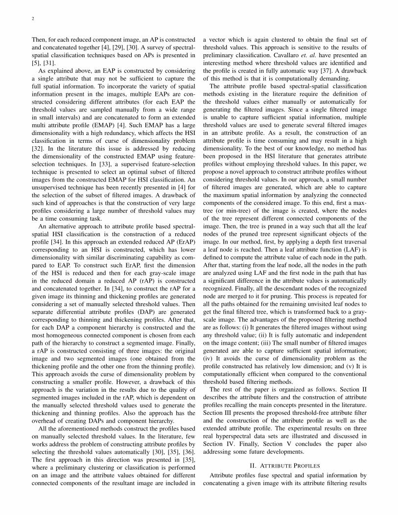
Gradient Curve (GC): To detect the suitable node on theconsidered path that is associated with the first significantdifference in attribute values, we compute the gradient fromthe leaf’s plotted position on the LAF curve (i.e., the startingpoint of the curve) to each of the break points on it. Pleasenote that the break points on the LAF curve represent thecorresponding attribute values for the intermediate nodes of theconsidered path. Fig. 4 shows an LAF curve where the dotted

5

Fig. 3. (a) Leaf attribute functions (LAF); (b) gradient curves (GC); (c) attribute ratio curves (ARC); and (d) maximal suitability curves (MSC) obtained byanalyzing three randomly selected paths from the max-tree. Each path is obtained from a randomly selected leaf node to the root node of the max-tree createdby considering 1st PC of University of Pavia data set.

Fig. 4. An LAF representing the attribute values in the path from a randomlyselected leaf node to the root. O is the starting position and R is the positionon LAF having maximum gradient from O.

lines help us in understanding the computation of gradientfor a break point from the starting position of the curve. Thegradient tan(θ) from the starting point O to a break point Rcan be computed as:

Gradient(OR) =RQ

OQ=

LAFNℓ(i) − LAFNℓ

(1)

i − 1(5)

where i is the position of a node on the path from Nℓ to theroot such that A(Ni) = R. A GC is created by calculating thegradient for each node on the path and is formally defined asfollows:

GCNℓ(i) =

{LAFNℓ

(i + 1) − LAFNℓ(1)

i

}, i = 1, 2, ..., P−1.

(6)Fig. 3(b) shows some gradient curves corresponding to the

LAFs illustrated in Fig. 3(a). From these figures one can

see that initially the gradient has an increasing behavior byincreasing the attribute value and reaches the maximum atthe node which has first significant difference in attributevalue. After that, the LAF keeps increasing trend whereas thegradient starts to decrease.

Attribute Ratio Curve (ARC): To detect the node that isassociated with a sudden change in the attribute values on theconsidered path, we propose to compute the ratio between theattribute value of a node and the attribute value of its childnode on the considered path. The ARC for a path associatedto the leaf node Nℓ can be computed as:

ARCNℓ(i) = log2

(LAFNℓ

(i + 1)

LAFNℓ(i)

), i = 1, 2, ..., P − 1.

(7)where i is the node number from the leaf to root and P isthe total number of nodes on the considered path. Fig. 3(c)shows few ARCs corresponding to the LAFs shown in Fig.3(a). From these figures one can see that an ARC has a localmaximum at the node that is associated with sudden changesin attribute values. Hence, ARC can be used to detect a nodeon the considered path which is responsible for such suddenchanges in attribute values.

3) Step 3 – Construction of MSC to detect node for treepruning: To detect the first node (starting from the leaf nodeon the considered path) that represents a significant object inthe image, a maximal suitability curve (MSC) is generated bycombining GC and ARC. The MSC for the leaf node Nℓ canbe defined as:

MSCNℓ(i) = GCNℓ

(i)·ARCNℓ(i), i = 1, 2, ..., P −1. (8)

6

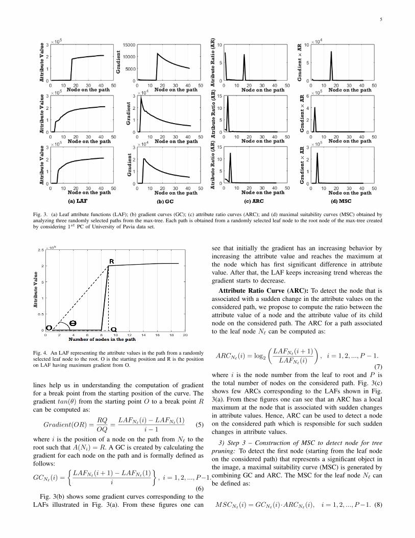
Fig. 5. A synthetic tree and the filtered trees obtained by the proposedtechnique after detecting a node (represented with filled circle) from the path(b) A to D (c) A to E and (d) A to G..

which can be written as:

(9)MSCNℓ

(i) =

(LAFNℓ

(i + 1) − LAFNℓ(1)

i

)

· log2

(LAFNℓ

(i + 1)

LAFNℓ(i)

)

From the above equation one can see that the MSC provideshigh values when both GC and ARC have high values. Fig.3(d) shows few maximal suitability curves corresponding tothe LAFs shown in Fig. 3(a). In our work the node on theconsidered path that is associated with the global maxima ofMSC is recognized as the node that represents a significantobject in the image.

4) Step 4 – Tree filtering: Once the node is detected on thepath, all its descendants are merged to it for pruning. Mergingmeans that all the pixels associated to the descendants are as-signed to the detected node. This is similar to the min strategyused for filtering [22]. In greater detail, Fig. 5 demonstrates theproposed tree filtering technique by considering the synthetictree shown in Fig. 5(a). First, a path from root node A to leafnode D (shown by the dashed line in Fig. 5(a)) is obtained foranalysis by using depth first traversal. From the path, if weassume that the node B is detected by our proposed techniquefor merging, then all the descendant nodes of B will be mergedto it and the obtained resultant tree is shown in Fig. 5 (b). Nowresuming the depth first traversal from B, a path from A toleaf node E (shown by the dashed line in Fig. 5(b)) is obtainedfor analysis. For this path, if B is the suitable node detectedby our technique, then after merging we get the tree shownin Fig. 5(c). Resuming the depth first traversal from B, a pathfrom A to leaf node G (shown by the dashed line in Fig.5(c)) is obtained for analysis. For this path, if we assume Fis the suitable node detected by the proposed technique, thenthe resultant tree obtained after merging its descendants is thatpresented in Fig. 5(d). Since at this point all the leaf nodesof the original tree are processed, the algorithm will stop andthe resultant tree is considered as filtered tree. The filteredtree is restituted back to a gray-scale image where all theconnected components of the given image have been filteredautomatically. For restitution, the same procedure is used asexplained in Subsection II-3. The proposed filtering techniqueis increasing, anti extensive and non idempotent in nature. Thesteps of the proposed attribute filtering method are shown inAlgorithm 1.

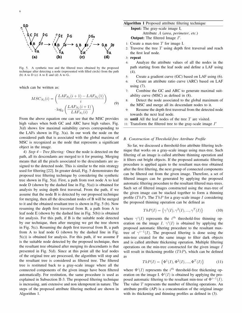
Algorithm 1 Proposed attribute filtering techniqueInput: The gray-scale image I,

Attribute A (area, perimeter, etc.)Output: The filtered Image I ′.

1: Create a max-tree T for image I.2: Traverse the tree T using depth first traversal and reach

the first leaf node.3: repeat4: Analyze the attribute values of all the nodes in the

path starting from the leaf node and define a LAF using(4).

5: Create a gradient curve (GC) based on LAF using (6).6: Create an attribute ratio curve (ARC) based on LAF

using (7).7: Combine the GC and ARC to generate maximal suit-

ability curve (MSC) as defined in (8).8: Detect the node associated to the global maximum of

the MSC and merge all its descendant nodes to it.9: Resume the depth first traversal from the detected node

towards the next leaf node.10: until All the leaf nodes of the tree T are visited.11: Transform the filtered tree to the gray-scale image I ′

B. Construction of Threshold-free Attribute Profile

So far, we discussed a threshold-free attribute filtering tech-nique that works on a gray-scale image using max-tree. Suchfiltering of an image is called attribute thinning operation andit filters out bright objects. If the proposed automatic filteringprocedure is applied again to the resultant max-tree obtainedafter the first filtering, the next group of connected componentscan be filtered out from the given image. Therefore, a set offiltered images can be generated by applying the proposedautomatic filtering procedure to the resultant filtered max-trees.Such set of filtered images constructed using the max-tree ofthe given image can be stacked together to form a thinningprofile (ThP ). The ThP for a gray-scale image I consideringthe proposed thinning operation can be defined as

ThP (I) ={γ1(I), γ2(I), ..., γT (I)

}(10)

where γi(I) represents the ith threshold-free thinning op-eration on the image I . γi(I) is obtained by applying theproposed automatic filtering procedure to the resultant max-tree of γi−1(I). The proposed filtering is done using themin-tree created for the same image to filter dark objectsand is called attribute thickening operation. Multiple filteringoperations on the min-tree constructed for the given image Iwill result in thickening profile (TkP ), which can be definedas

TkP (I) ={Φ1(I), Φ2(I), ...,ΦT (I)

}(11)

where Φi(I) represents the ith threshold-free thickening op-eration on the image I. Φi(I) is obtained by applying the pro-posed automatic filtering to the resultant min-tree of Φi−1(I).The value T represents the number of filtering operations. Anattribute profile (AP) is a concatenation of the original imagewith its thickening and thinning profiles as defined in (3).

7

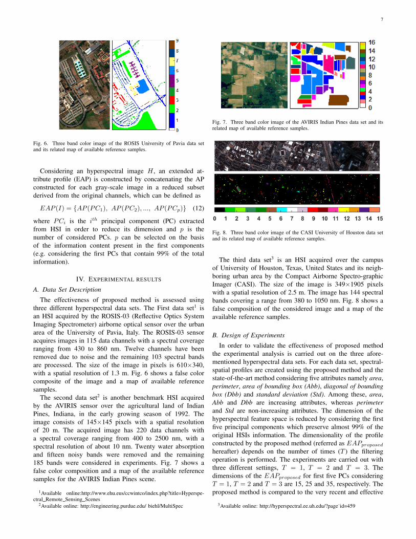
Fig. 6. Three band color image of the ROSIS University of Pavia data setand its related map of available reference samples.

Considering an hyperspectral image H , an extended at-tribute profile (EAP) is constructed by concatenating the APconstructed for each gray-scale image in a reduced subsetderived from the original channels, which can be defined as

EAP (I) = {AP (PC1), AP (PC2), ..., AP (PCp)} (12)

where PCi is the ith principal component (PC) extractedfrom HSI in order to reduce its dimension and p is thenumber of considered PCs. p can be selected on the basisof the information content present in the first components(e.g. considering the first PCs that contain 99% of the totalinformation).

IV. EXPERIMENTAL RESULTS

A. Data Set Description

The effectiveness of proposed method is assessed usingthree different hyperspectral data sets. The First data set1 isan HSI acquired by the ROSIS-03 (Reflective Optics SystemImaging Spectrometer) airborne optical sensor over the urbanarea of the University of Pavia, Italy. The ROSIS-03 sensoracquires images in 115 data channels with a spectral coverageranging from 430 to 860 nm. Twelve channels have beenremoved due to noise and the remaining 103 spectral bandsare processed. The size of the image in pixels is 610×340,with a spatial resolution of 1.3 m. Fig. 6 shows a false colorcomposite of the image and a map of available referencesamples.

The second data set2 is another benchmark HSI acquiredby the AVIRIS sensor over the agricultural land of IndianPines, Indiana, in the early growing season of 1992. Theimage consists of 145×145 pixels with a spatial resolutionof 20 m. The acquired image has 220 data channels witha spectral coverage ranging from 400 to 2500 nm, with aspectral resolution of about 10 nm. Twenty water absorptionand fifteen noisy bands were removed and the remaining185 bands were considered in experiments. Fig. 7 shows afalse color composition and a map of the available referencesamples for the AVIRIS Indian Pines scene.

1Available online:http://www.ehu.eus/ccwintco/index.php?title=Hyperspe-ctral Remote Sensing Scenes

2Available online: http://engineering.purdue.edu/ biehl/MultiSpec

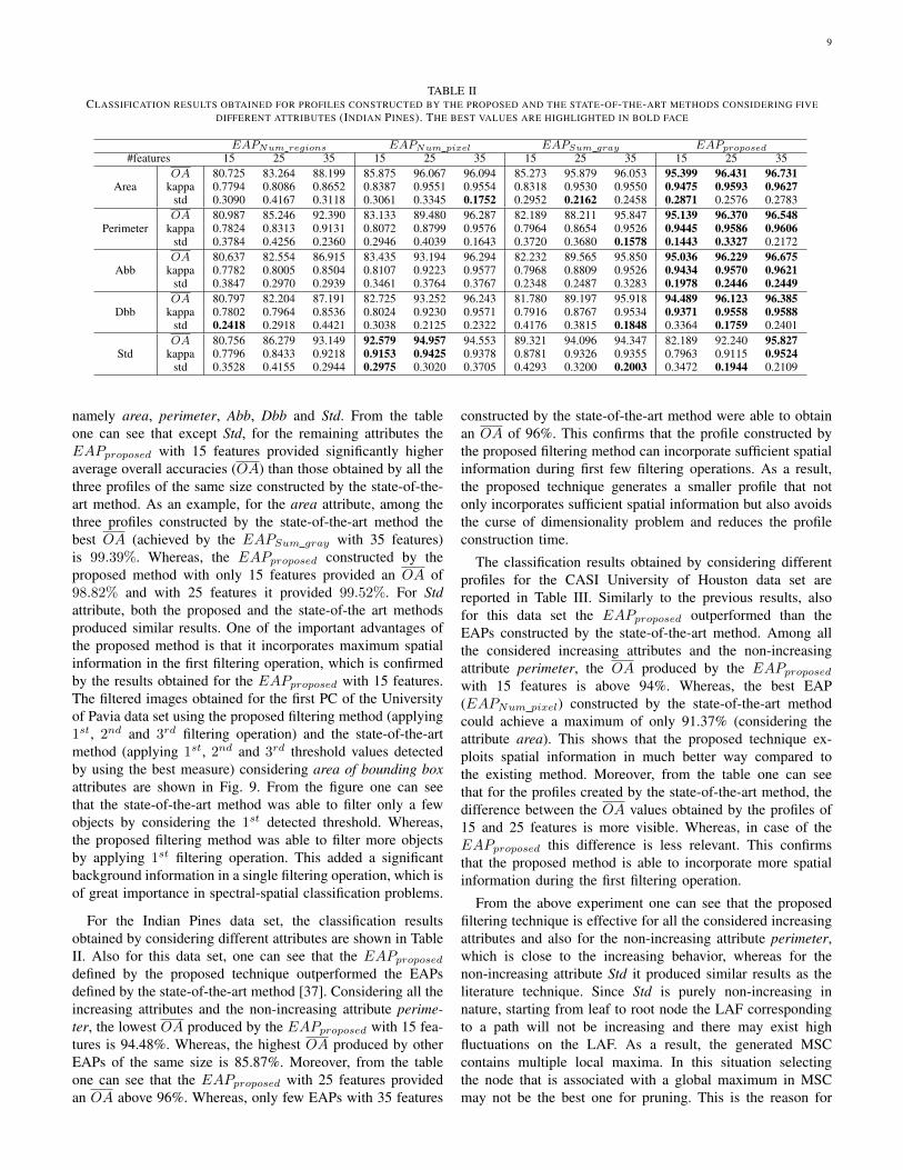
Fig. 7. Three band color image of the AVIRIS Indian Pines data set and itsrelated map of available reference samples.

Fig. 8. Three band color image of the CASI University of Houston data setand its related map of available reference samples.

The third data set3 is an HSI acquired over the campusof University of Houston, Texas, United States and its neigh-boring urban area by the Compact Airborne Spectro-graphicImager (CASI). The size of the image is 349×1905 pixelswith a spatial resolution of 2.5 m. The image has 144 spectralbands covering a range from 380 to 1050 nm. Fig. 8 shows afalse composition of the considered image and a map of theavailable reference samples.

B. Design of Experiments

In order to validate the effectiveness of proposed methodthe experimental analysis is carried out on the three afore-mentioned hyperspectral data sets. For each data set, spectral-spatial profiles are created using the proposed method and thestate-of-the-art method considering five attributes namely area,perimeter, area of bounding box (Abb), diagonal of boundingbox (Dbb) and standard deviation (Std). Among these, area,Abb and Dbb are increasing attributes, whereas perimeterand Std are non-increasing attributes. The dimension of thehyperspectral feature space is reduced by considering the firstfive principal components which preserve almost 99% of theoriginal HSIs information. The dimensionality of the profileconstructed by the proposed method (referred as EAPproposed

hereafter) depends on the number of times (T ) the filteringoperation is performed. The experiments are carried out withthree different settings, T = 1, T = 2 and T = 3. Thedimensions of the EAPproposed for first five PCs consideringT = 1, T = 2 and T = 3 are 15, 25 and 35, respectively. Theproposed method is compared to the very recent and effective

3Available online: http://hyperspectral.ee.uh.edu/?page˙id=459

8

TABLE ICLASSIFICATION RESULTS OBTAINED FOR PROFILES CONSTRUCTED BY THE PROPOSED AND THE STATE-OF-THE-ART METHODS CONSIDERING FIVE

DIFFERENT ATTRIBUTES (UNIVERSITY OF PAVIA). THE BEST VALUES ARE HIGHLIGHTED IN BOLD FACE

EAPNum regions EAPNum pixel EAPSum gray EAPproposed

#features 15 25 35 15 25 35 15 25 35 15 25 35

AreaOA 87.012 89.550 92.544 93.125 99.319 99.327 90.017 98.851 99.395 98.818 99.519 99.632

kappa 0.8243 0.8595 0.9006 0.9084 0.9910 0.9911 0.8660 0.9848 0.9920 0.9843 0.9936 0.9951std 0.0721 0.1215 0.1121 0.0896 0.0539 0.0510 0.1325 0.0752 0.0360 0.0561 0.0408 0.0441

PerimeterOA 87.259 89.388 92.726 89.217 93.777 98.929 88.750 93.292 98.590 98.937 99.418 99.496

kappa 0.8278 0.8573 0.9030 0.8550 0.9172 0.9858 0.8484 0.9107 0.9813 0.9859 0.9923 0.9933std 0.1336 0.1538 0.0634 0.1359 0.1095 0.0394 0.1344 0.0712 0.0504 0.0608 0.0380 0.0486

AbbOA 86.891 89.041 91.642 89.286 97.319 99.555 88.643 96.095 99.415 98.628 99.315 99.600

kappa 0.8226 0.8525 0.8882 0.8559 0.9644 0.9941 0.8471 0.9482 0.9922 0.9818 0.9909 0.9947std 0.1685 0.1160 0.0800 0.1538 0.0516 0.0529 0.1742 0.1096 0.0659 0.0800 0.0406 0.0481

DbbOA 86.807 88.883 91.421 89.261 96.718 99.545 88.668 95.016 99.310 97.751 99.019 99.673

kappa 0.8216 0.8503 0.8852 0.8556 0.9564 0.9940 0.8475 0.9338 0.9908 0.9701 0.9870 0.9957std 0.0904 0.1037 0.0878 0.1306 0.0942 0.0333 0.2022 0.1086 0.0279 0.0732 0.0734 0.0599

StdOA 86.878 88.984 91.644 89.292 97.289 99.567 88.668 96.057 99.358 88.280 95.176 98.074

kappa 0.8225 0.8518 0.8882 0.8559 0.9640 0.9943 0.8474 0.9476 0.9915 0.8421 0.9358 0.9745std 0.1657 0.1569 0.1111 0.0773 0.0820 0.0396 0.0892 0.0602 0.0562 0.1421 0.0785 0.0963

Fig. 9. Filtered images obtained by applying the state-of-the-art and the proposed filtering method to the 1st principal component of the University ofPavia data set by considering the area of bounding box attribute. The best filtered image obtained by the state-of-the-art method [37] considering (a) the 1st

threshold, (b) the 2nd threshold and (c) the 3rd threshold. The filtered image obtained by the proposed method after applying (d) the 1st, (e) the 2nd and(f) the 3rd filtering operation.

state-of-the-art method presented in [37], which creates EAPusing a set of automatically detected threshold values. Forthe detection of such thresholds, the method first exploitsthe tree structure and generates a large number of thresholdvalues automatically. Then, a vector called GCF is created thatstores a measure computed corresponding to each thresholdvalue. The measures used in [37] are number of changedregions, number of changed pixels and sum of gray-levelvalues. The created GCF is approximated using regression andbreak points of the approximated curve are referred as finaldetected threshold values. Finally, considering the same PCsas used by our method, the EAP is constructed by applyingthe automatically detected threshold values.

The spectral-spatial profiles constructed by the state-of-the-art method considering the number of changed regions, thenumber of changed pixels and the sum of gray-level valuesare referred in this paper as EAPNum regions, EAPNum pixel

and EAPSum gray , respectively. For a fair comparison, theseprofiles are also constructed with the same number of features(images) as those of the EAPproposed. A one-against-allsupport vector machine (SVM) classifier with radial-basis-function (RBF) kernel is used for classification purposes. The

SVM parameters are obtained by performing grid search with5-fold cross-validation. In the experiments, ten separate pairsof the training and test sets are generated, each of which iscomposed of a training set having 30% of the labeled samplesrandomly selected from each class and a test set having the rest70% of the samples. The classification results are reported interms of average overall accuracy (OA), the related standarddeviation (std) and the average kappa accuracy (kappa). Allthe algorithms are implemented in MATLAB (R2015a) andthe SVM classifier is implemented using the LIBSVM library[41]. However, note that any classifier can be used for classi-fying the constructed attribute profiles, which are general andclassifier independent. The regression is implemented usingthe code available in [42].

C. ResultsTo evaluate the effectiveness of the attribute profiles con-

structed by the proposed method (EAPproposed), the firstexperimental analysis is carried out on the University of Paviadata set. Table I reports the classification results obtained forthe EAPproposed, the EAPNum regions, the EAPNum pixel

and the EAPSum gray considering five different attributes

9

TABLE IICLASSIFICATION RESULTS OBTAINED FOR PROFILES CONSTRUCTED BY THE PROPOSED AND THE STATE-OF-THE-ART METHODS CONSIDERING FIVE

DIFFERENT ATTRIBUTES (INDIAN PINES). THE BEST VALUES ARE HIGHLIGHTED IN BOLD FACE

EAPNum regions EAPNum pixel EAPSum gray EAPproposed

#features 15 25 35 15 25 35 15 25 35 15 25 35

AreaOA 80.725 83.264 88.199 85.875 96.067 96.094 85.273 95.879 96.053 95.399 96.431 96.731

kappa 0.7794 0.8086 0.8652 0.8387 0.9551 0.9554 0.8318 0.9530 0.9550 0.9475 0.9593 0.9627std 0.3090 0.4167 0.3118 0.3061 0.3345 0.1752 0.2952 0.2162 0.2458 0.2871 0.2576 0.2783

PerimeterOA 80.987 85.246 92.390 83.133 89.480 96.287 82.189 88.211 95.847 95.139 96.370 96.548

kappa 0.7824 0.8313 0.9131 0.8072 0.8799 0.9576 0.7964 0.8654 0.9526 0.9445 0.9586 0.9606std 0.3784 0.4256 0.2360 0.2946 0.4039 0.1643 0.3720 0.3680 0.1578 0.1443 0.3327 0.2172

AbbOA 80.637 82.554 86.915 83.435 93.194 96.294 82.232 89.565 95.850 95.036 96.229 96.675

kappa 0.7782 0.8005 0.8504 0.8107 0.9223 0.9577 0.7968 0.8809 0.9526 0.9434 0.9570 0.9621std 0.3847 0.2970 0.2939 0.3461 0.3764 0.3767 0.2348 0.2487 0.3283 0.1978 0.2446 0.2449

DbbOA 80.797 82.204 87.191 82.725 93.252 96.243 81.780 89.197 95.918 94.489 96.123 96.385

kappa 0.7802 0.7964 0.8536 0.8024 0.9230 0.9571 0.7916 0.8767 0.9534 0.9371 0.9558 0.9588std 0.2418 0.2918 0.4421 0.3038 0.2125 0.2322 0.4176 0.3815 0.1848 0.3364 0.1759 0.2401

StdOA 80.756 86.279 93.149 92.579 94.957 94.553 89.321 94.096 94.347 82.189 92.240 95.827

kappa 0.7796 0.8433 0.9218 0.9153 0.9425 0.9378 0.8781 0.9326 0.9355 0.7963 0.9115 0.9524std 0.3528 0.4155 0.2944 0.2975 0.3020 0.3705 0.4293 0.3200 0.2003 0.3472 0.1944 0.2109

namely area, perimeter, Abb, Dbb and Std. From the tableone can see that except Std, for the remaining attributes theEAPproposed with 15 features provided significantly higheraverage overall accuracies (OA) than those obtained by all thethree profiles of the same size constructed by the state-of-the-art method. As an example, for the area attribute, among thethree profiles constructed by the state-of-the-art method thebest OA (achieved by the EAPSum gray with 35 features)is 99.39%. Whereas, the EAPproposed constructed by theproposed method with only 15 features provided an OA of98.82% and with 25 features it provided 99.52%. For Stdattribute, both the proposed and the state-of-the art methodsproduced similar results. One of the important advantages ofthe proposed method is that it incorporates maximum spatialinformation in the first filtering operation, which is confirmedby the results obtained for the EAPproposed with 15 features.The filtered images obtained for the first PC of the Universityof Pavia data set using the proposed filtering method (applying1st, 2nd and 3rd filtering operation) and the state-of-the-artmethod (applying 1st, 2nd and 3rd threshold values detectedby using the best measure) considering area of bounding boxattributes are shown in Fig. 9. From the figure one can seethat the state-of-the-art method was able to filter only a fewobjects by considering the 1st detected threshold. Whereas,the proposed filtering method was able to filter more objectsby applying 1st filtering operation. This added a significantbackground information in a single filtering operation, which isof great importance in spectral-spatial classification problems.

For the Indian Pines data set, the classification resultsobtained by considering different attributes are shown in TableII. Also for this data set, one can see that the EAPproposed

defined by the proposed technique outperformed the EAPsdefined by the state-of-the-art method [37]. Considering all theincreasing attributes and the non-increasing attribute perime-ter, the lowest OA produced by the EAPproposed with 15 fea-tures is 94.48%. Whereas, the highest OA produced by otherEAPs of the same size is 85.87%. Moreover, from the tableone can see that the EAPproposed with 25 features providedan OA above 96%. Whereas, only few EAPs with 35 features

constructed by the state-of-the-art method were able to obtainan OA of 96%. This confirms that the profile constructed bythe proposed filtering method can incorporate sufficient spatialinformation during first few filtering operations. As a result,the proposed technique generates a smaller profile that notonly incorporates sufficient spatial information but also avoidsthe curse of dimensionality problem and reduces the profileconstruction time.

The classification results obtained by considering differentprofiles for the CASI University of Houston data set arereported in Table III. Similarly to the previous results, alsofor this data set the EAPproposed outperformed than theEAPs constructed by the state-of-the-art method. Among allthe considered increasing attributes and the non-increasingattribute perimeter, the OA produced by the EAPproposed

with 15 features is above 94%. Whereas, the best EAP(EAPNum pixel) constructed by the state-of-the-art methodcould achieve a maximum of only 91.37% (considering theattribute area). This shows that the proposed technique ex-ploits spatial information in much better way compared tothe existing method. Moreover, from the table one can seethat for the profiles created by the state-of-the-art method, thedifference between the OA values obtained by the profiles of15 and 25 features is more visible. Whereas, in case of theEAPproposed this difference is less relevant. This confirmsthat the proposed method is able to incorporate more spatialinformation during the first filtering operation.

From the above experiment one can see that the proposedfiltering technique is effective for all the considered increasingattributes and also for the non-increasing attribute perimeter,which is close to the increasing behavior, whereas for thenon-increasing attribute Std it produced similar results as theliterature technique. Since Std is purely non-increasing innature, starting from leaf to root node the LAF correspondingto a path will not be increasing and there may exist highfluctuations on the LAF. As a result, the generated MSCcontains multiple local maxima. In this situation selectingthe node that is associated with a global maximum in MSCmay not be the best one for pruning. This is the reason for

10

TABLE IIICLASSIFICATION RESULTS OBTAINED FOR PROFILES CONSTRUCTED BY THE PROPOSED AND THE STATE-OF-THE-ART METHODS CONSIDERING FIVE

DIFFERENT ATTRIBUTES (UNIVERSITY OF HOUSTON). THE BEST VALUES ARE HIGHLIGHTED IN BOLD FACE

EAPNum regions EAPNum pixel EAPSum gray EAPproposed

#features 15 25 35 15 25 35 15 25 35 15 25 35

AreaOA 86.576 88.734 91.544 91.368 96.924 97.568 90.329 95.353 96.825 95.684 96.970 97.793

kappa 0.8548 0.8782 0.9086 0.9067 0.9667 0.9737 0.8954 0.9498 0.9657 0.9533 0.9672 0.9761std 0.2963 0.3396 0.1882 0.2066 0.1874 0.1863 0.2029 0.2703 0.2830 0.1742 0.1495 0.1884

PerimeterOA 86.837 88.799 91.344 89.983 93.629 96.743 89.235 93.205 96.621 94.582 95.993 97.169

kappa 0.8576 0.8789 0.9064 0.8917 0.9311 0.9648 0.8836 0.9265 0.9635 0.9414 0.9567 0.9694std 0.1580 0.2299 0.4229 0.1410 0.2501 0.1708 0.3684 0.2472 0.1681 0.1692 0.1821 0.1566

AbbOA 86.404 88.528 90.780 89.495 93.646 97.230 88.863 93.378 97.451 95.163 96.951 97.838

kappa 0.8529 0.8759 0.9003 0.8864 0.9313 0.9701 0.8796 0.9284 0.9724 0.9477 0.9670 0.9766std 0.3673 0.2907 0.2003 0.2287 0.2802 0.2131 0.2282 0.1740 0.2108 0.3042 0.1439 0.1511

DbbOA 86.409 88.563 90.932 89.426 93.679 97.356 88.231 91.485 96.461 94.103 97.140 97.742

kappa 0.8530 0.8763 0.9019 0.8857 0.9316 0.9714 0.8727 0.9079 0.9617 0.9362 0.9691 0.9756std 0.3811 0.1815 0.2598 0.3018 0.3395 0.1580 0.1837 0.2106 0.2470 0.1676 0.1905 0.1990

StdOA 86.409 91.288 94.891 91.990 95.056 95.854 87.413 93.256 95.530 88.233 93.507 95.451

kappa 0.8530 0.9058 0.9447 0.9134 0.9465 0.9551 0.8638 0.9270 0.9517 0.8727 0.9298 0.9508std 0.3811 0.2117 0.3947 0.2270 0.2271 0.2672 0.2569 0.1581 0.2047 0.3094 0.2333 0.1480

which the proposed technique produced lower accuracies forthe Std attribute as compared to the other considered attributes.Nonetheless, it still provided similar results as those producedby the considered state-of-the-art method.

To further assess the effectiveness of the proposed method,the classification results obtained by using the proposedprofiles (EAPproposed) with 35 features are also comparedto some recent spectral-spatial classification techniques suchas EMEP, UNMIXING + SRC (referred as USRC), SRC,JSRC, MASR, SBSDM, SAS and CNN presented in [5]. Theexperiment is conducted on the CASI University of Houstondata set considering the standard training and test set madeavailable by the IEEE GRSS data fusion committee 2013. Forthis experiment, exactly the same experimental settings as usedin [5] including the use of the random forest classifier with200 trees are considered for classification of the constructedEAPproposed. The classification results reported in Table IVshow that the proposed technique outperforms many of thespectral-spatial classification techniques presented in [5]. Thisagain shows the potentiality of proposed method for spectral-spatial classification of HSIs.

D. Results: Computational Time

In order to assess the effectiveness of the proposed tech-nique in terms of computational time, Table V reports the times(in seconds) required by the proposed and the state-of-the-art method presented in [37] for the construction of differentprofiles having 35 features. Both the algorithms are imple-mented in MATLAB (R2015a) and tested on a workstationwith Intel(R) Xeon(R) processor having 3.60 GHz processingpower and 16 GB RAM. The time required for generating pro-files EAPNum regions, EAPNum pixel, EAPSum gray andEAPproposed is denoted as TNR, TNP , TSG and Tprpsd,respectively. From the table one can see that the proposedmethod can generate filtered images in an at least 50 timesfaster time than the state-of-the-art method. Moreover, forthe Std attribute the proposed technique is extremely efficientin terms of computational time. Compared to the proposedtechnique, the technique presented in [37] requires more

TABLE VCOMPUTATIONAL TIME IN SECONDS REQUIRED FOR CONSTRUCTING

SPECTRAL-SPATIAL PROFILES OF SIZE 35 USING THE STATE-OF-THE-ARTMETHOD AND THE PROPOSED METHOD

Data set Attribute TNR TNP TSG Tprpsd

Universityof Pavia

Area 3979 4148 4156 65Perimeter 2508 2490 2488 70

Abb 3054 3143 3154 79Dbb 3636 3686 3646 80Std 795807 802349 816577 132

IndianPines

Area 874 869 854 6Perimeter 519 521 528 6

Abb 320 317 318 6Dbb 384 377 393 6Std 30859 31349 31442 44

Universityof Houston

Area 8068 8258 8253 368Perimeter 4240 4321 4316 339

Abb 6282 6171 6175 371Dbb 7525 6181 7632 330Std 1097565 1007517 1087365 631

time because: (i) it creates GCF by evaluating a measurecorresponding to a large number of possible threshold values;and (ii) it uses regression for approximating the GCF whichrequires a significant amount of time that is sensitive to thenumber of initial thresholds identified from the tree. On theother hand, the proposed filtering method has no such burdenfor threshold detection and the tree is filtered by applying onlyone depth first traversal.

V. CONCLUSION

Attribute profiles for spectral-spatial classification existingin the literature detect threshold values either manually orautomatically for generating the filtered images. Usually, sincea single filtered image is unable to capture sufficient spatialinformation, multiple threshold values are used and severalfiltered images are generated. As a result, the constructionof an attribute profile is time consuming and may result ina large number of features. To the best of our knowledgeno method exists in the HSI literature that generate attributeprofiles without employing threshold values. In this paper wehave proposed a novel approach that generates the filtered

11

TABLE IVOVERALL ACCURACY (OA), AVERAGE CLASSWISE-ACCURACY (AA) AND KAPPA COEFFICIENT (KAPPA) PROVIDED BY THE PROPOSED AND SEVERAL

RECENT STATE-OF-THE-ART SPECTRAL-SPATIAL CLASSIFICATION METHODS USING STANDARD TRAINING AND TEST SETS. (UNIVERSITY OF HOUSTONDATA SET)

Proposed Technique Different Spectral-Spatial TechniquesAccuracies Area Perimeter Abb Dbb Std EMEP USRC SRC JSRC MASR SBSDM SAS CNN

OA 82.52 82.91 82.93 82.80 82.95 80.83 70.49 73.37 76.35 77.04 75.66 75.72 82.75AA 85.43 85.33 85.30 85.23 85.38 83.64 77.25 78.35 78.35 79.74 78.26 78.08 84.04

kappa 0.8105 0.8149 0.8150 0.8136 0.8152 0.7920 0.6802 0.7128 0.7446 0.7520 0.7371 0.7376 0.8061

images for constructing attribute profiles without using thethreshold values. The proposed filtering approach creates atree to process connected components of the image and theinsignificant objects are merged to their background objects.To this end, the path from the root to a leaf node is obtainedusing depth first traversal and a leaf attribute function (LAF)is defined to compute the attribute values of each node onthe path. Then a novel criterion is defined to automaticallydetect the node on the path where the attribute values havefirst significant difference compared to its descendant nodes.Finally, all the descendants of the detected node are mergedto it. The process is repeated for each path correspondingto the unvisited leaf nodes of the tree to generate the finalfiltered tree, which is transformed back to a filtered image.The proposed filtering method is repeated to generate multiplefiltered images for constructing the attribute profiles.

In order to show the effectiveness of the proposed technique,the spectral-spatial profiles constructed by the proposed and astate-of-the-art method are compared on three hyperspectralimages using five different attributes. The comparison showedthat the proposed method has several advantages: (i) It gener-ates filtered images without using any threshold value; (ii) It isfully automatic and independent on the image content; (iii) Asmall number of filtered images generated by this method arecapable to capture a large amount of spatial information; (iv) Itis more robust to handle curse of dimensionality problem; and(v) It generate the profiles in much faster way. Moreover, theproposed technique produces comparable classification results(some times better) with the different recent spectral-spatialclassification techniques presented in the literature [5].

Although the proposed approach significantly reduced thecomputational time for profile generation, as a future work theproposed technique will be implemented in parallel processingenvironment to further increase its computational speed.

ACKNOWLEDGMENTS

The authors would like to thank the anonymous referees fortheir constructive criticism and valuable suggestions. The au-thors would also like to thank Dr. Saurabh Prasad, Universityof Houston for providing the Houston data set. This work issupported in part by a RPS-NER research grant from All IndiaCouncil for Technical Education, New Delhi.

REFERENCES

[1] C.-I. Chang, Hyperspectral data exploitation: theory and applications.Hoboken, NJ, USA: John Wiley & Sons, 2007.

[2] H. J. Kramer, Observation of the Earth and its Environment: Survey ofMissions and Sensors. New York, USA: Springer, 2002.

[3] F. Melgani and L. Bruzzone, “Classification of hyperspectral remotesensing images with support vector machines,” IEEE Transactions ongeoscience and remote sensing, vol. 42, no. 8, pp. 1778–1790, 2004.

[4] K. Bhardwaj and S. Patra, “An unsupervised technique for optimalfeature selection in attribute profiles for spectral-spatial classification ofhyperspectral images,” ISPRS Journal of Photogrammetry and RemoteSensing, vol. 138, pp. 139–150, 2018.

[5] P. Ghamisi, E. Maggiori, S. Li, R. Souza, Y. Tarablaka, G. Moser,A. De Giorgi, L. Fang, Y. Chen, M. Chi et al., “New frontiers in spectral-spatial hyperspectral image classification: The latest advances basedon mathematical morphology, markov random fields, segmentation,sparse representation, and deep learning,” IEEE Geoscience and RemoteSensing Magazine, vol. 6, no. 3, pp. 10–43, 2018.

[6] Y. Chen, N. M. Nasrabadi, and T. D. Tran, “Hyperspectral image classi-fication using dictionary-based sparse representation,” IEEE transactionson geoscience and remote sensing, vol. 49, no. 10, pp. 3973–3985, 2011.

[7] W. Fu, S. Li, L. Fang, X. Kang, and J. A. Benediktsson, “Hyperspectralimage classification via shape-adaptive joint sparse representation,”IEEE Journal of Selected Topics in Applied Earth Observations andRemote Sensing, vol. 9, no. 2, pp. 556–567, 2016.

[8] L. Fang, S. Li, X. Kang, and J. A. Benediktsson, “Spectral–spatialhyperspectral image classification via multiscale adaptive sparse rep-resentation,” IEEE Transactions on Geoscience and Remote Sensing,vol. 52, no. 12, pp. 7738–7749, 2014.

[9] M.-D. Iordache, J. M. Bioucas-Dias, and A. Plaza, “Sparse unmixingof hyperspectral data,” IEEE Transactions on Geoscience and RemoteSensing, vol. 49, no. 6, pp. 2014–2039, 2011.

[10] L. Fang, S. Li, X. Kang, and J. A. Benediktsson, “Spectral–spatial clas-sification of hyperspectral images with a superpixel-based discriminativesparse model,” IEEE Transactions on Geoscience and Remote Sensing,vol. 53, no. 8, pp. 4186–4201, 2015.

[11] Y. Chen, H. Jiang, C. Li, X. Jia, and P. Ghamisi, “Deep feature extractionand classification of hyperspectral images based on convolutional neuralnetworks,” IEEE Transactions on Geoscience and Remote Sensing,vol. 54, no. 10, pp. 6232–6251, 2016.

[12] S. Hao, W. Wang, Y. Ye, E. Li, and L. Bruzzone, “A deep networkarchitecture for super-resolution-aided hyperspectral image classificationwith classwise loss,” IEEE Transactions on Geoscience and RemoteSensing, vol. 56, no. 8, pp. 4650–4663, 2018.

[13] S. Hao, W. Wang, Y. Ye, T. Nie, and L. Bruzzone, “Two-stream deeparchitecture for hyperspectral image classification,” IEEE Transactionson Geoscience and Remote Sensing, vol. 56, no. 4, pp. 2349–2361, 2018.

[14] J. A. Benediktsson, J. A. Palmason, and J. R. Sveinsson, “Classificationof hyperspectral data from urban areas based on extended morpholog-ical profiles,” IEEE Transactions on Geoscience and Remote Sensing,vol. 43, no. 3, pp. 480–491, 2005.

[15] J. Serra, Image analysis and mathematical morphology. London:Academic Press, 1982.

[16] J. Serra and L. Vincent, “An overview of morphological filtering,”Circuits, Systems, and Signal Processing, vol. 11, no. 1, pp. 47–108,1992.

[17] J. A. Benediktsson, M. Pesaresi, and K. Amason, “Classification andfeature extraction for remote sensing images from urban areas based onmorphological transformations,” IEEE Transactions on Geoscience andRemote Sensing, vol. 41, no. 9, pp. 1940–1949, 2003.

[18] S. Patra, K. Bhardwaj, and L. Bruzzone, “A spectral-spatial multicriteriaactive learning technique for hyperspectral image classification,” IEEEJournal of Selected Topics in Applied Earth Observations and RemoteSensing, vol. 10, no. 12, pp. 5213–5227, 2017.

[19] M. Dalla Mura, J. A. Benediktsson, B. Waske, and L. Bruzzone,“Morphological attribute profiles for the analysis of very high resolutionimages,” IEEE Transactions on Geoscience and Remote Sensing, vol. 48,no. 10, pp. 3747–3762, 2010.

12

[20] L. Vincent, “Grayscale area openings and closings, their efficient im-plementation and applications,” in First Workshop on MathematicalMorphology and its Applications to Signal Processing, 1993, pp. 22–27.

[21] E. J. Breen and R. Jones, “Attribute openings, thinnings, and granulome-tries,” Computer Vision and Image Understanding, vol. 64, no. 3, pp.377–389, 1996.

[22] P. Salembier, A. Oliveras, and L. Garrido, “Antiextensive connectedoperators for image and sequence processing,” IEEE Transactions onImage Processing, vol. 7, no. 4, pp. 555–570, 1998.

[23] B. Song, J. Li, M. Dalla Mura, P. Li, A. Plaza, J. M. Bioucas-Dias, J. A.Benediktsson, and J. Chanussot, “Remotely sensed image classificationusing sparse representations of morphological attribute profiles,” IEEEtransactions on geoscience and remote sensing, vol. 52, no. 8, pp. 5122–5136, 2014.

[24] J. Xia, M. Dalla Mura, J. Chanussot, P. Du, and X. He, “Randomsubspace ensembles for hyperspectral image classification with extendedmorphological attribute profiles,” IEEE Transactions on Geoscience andRemote Sensing, vol. 53, no. 9, pp. 4768–4786, 2015.

[25] B. Demir and L. Bruzzone, “Histogram-based attribute profiles forclassification of very high resolution remote sensing images,” IEEETransactions on Geoscience and Remote Sensing, vol. 54, no. 4, pp.2096–2107, 2016.

[26] Z. Zhang and M. M. Crawford, “A batch-mode regularized multimetricactive learning framework for classification of hyperspectral images,”IEEE Transactions on Geoscience and Remote Sensing, vol. 55, no. 11,pp. 6594 – 6609, 2017.

[27] A. Das, K. Bhardwaj, and S. Patra, “Morphological complexity profilefor the analysis of hyperspectral images,” in 2018 4th InternationalConference on Recent Advances in Information Technology (RAIT).IEEE, 2018, pp. 1–6.

[28] M. Dalla Mura, J. A. Benediktsson, B. Waske, and L. Bruzzone,“Extended profiles with morphological attribute filters for the analysisof hyperspectral data,” International Journal of Remote Sensing, vol. 31,no. 22, pp. 5975–5991, 2010.

[29] P. R. Marpu, M. Pedergnana, M. Dalla Mura, S. Peeters, J. A. Benedik-tsson, and L. Bruzzone, “Classification of hyperspectral data usingextended attribute profiles based on supervised and unsupervised featureextraction techniques,” International Journal of Image and Data Fusion,vol. 3, no. 3, pp. 269–298, 2012.

[30] P. Ghamisi, J. A. Benediktsson, and J. R. Sveinsson, “Automaticspectral–spatial classification framework based on attribute profiles andsupervised feature extraction,” IEEE Transactions on Geoscience andRemote Sensing, vol. 52, no. 9, pp. 5771–5782, 2014.

[31] P. Ghamisi, M. Dalla Mura, and J. A. Benediktsson, “A survey onspectral–spatial classification techniques based on attribute profiles,”IEEE Transactions on Geoscience and Remote Sensing, vol. 53, no. 5,pp. 2335–2353, 2015.

[32] G. Hughes, “On the mean accuracy of statistical pattern recognizers,”IEEE transactions on information theory, vol. 14, no. 1, pp. 55–63,1968.

[33] M. Pedergnana, P. R. Marpu, M. Dalla Mura, J. A. Benediktsson, andL. Bruzzone, “A novel technique for optimal feature selection in attributeprofiles based on genetic algorithms,” IEEE Transactions on Geoscienceand Remote Sensing, vol. 51, no. 6, pp. 3514–3528, 2013.

[34] N. Falco, J. A. Benediktsson, and L. Bruzzone, “Spectral and spatialclassification of hyperspectral images based on ICA and reduced mor-phological attribute profiles,” IEEE Transactions on Geoscience andRemote Sensing, vol. 53, no. 11, pp. 6223–6240, 2015.

[35] Z. Mahmood, G. Thoonen, and P. Scheunders, “Automatic threshold se-lection for morphological attribute profiles,” in Geoscience and RemoteSensing Symposium (IGARSS), 2012 IEEE International. IEEE, 2012,pp. 4946–4949.

[36] P. R. Marpu, M. Pedergnana, M. Dalla Mura, J. A. Benediktsson,and L. Bruzzone, “Automatic generation of standard deviation attributeprofiles for spectral–spatial classification of remote sensing data,” IEEEGeoscience and Remote Sensing Letters, vol. 10, no. 2, pp. 293–297,2013.

[37] G. Cavallaro, N. Falco, M. Dalla Mura, and J. A. Benediktsson,“Automatic attribute profiles,” IEEE Transactions on Image Processing,vol. 26, no. 4, pp. 1859–1872, 2017.

[38] E. Carlinet and T. Geraud, “A comparative review of componenttree computation algorithms,” IEEE Transactions on Image Processing,vol. 23, no. 9, pp. 3885–3895, 2014.

[39] P. Bosilj, E. Kijak, and S. Lefevre, “Partition and inclusion hierarchiesof images: A comprehensive survey,” Journal of Imaging, vol. 4, no. 2,p. 33, 2018.

[40] L. Najman and M. Couprie, “Building the component tree in quasi-linear time,” IEEE Transactions on image processing, vol. 15, no. 11,pp. 3531–3539, 2006.

[41] C.-C. Chang and C.-J. Lin, “LIBSVM: a library for support vectormachines,” ACM Transactions on Intelligent Systems and Technology(TIST), vol. 2, no. 3, p. 27, 2011.

[42] D. Lemire, “A better alternative to piecewise linear time series segmen-tation,” in Proceedings of the 2007 SIAM International Conference onData Mining. SIAM, 2007, pp. 545–550.