c 2012 Anqi Shao - University of Floridaufdcimages.uflib.ufl.edu/UF/E0/04/39/21/00001/SHAO__.pdf ·...

A FAST AND EXACT SIMULATION FOR CIR PROCESS

By

ANQI SHAO

A DISSERTATION PRESENTED TO THE GRADUATE SCHOOLOF THE UNIVERSITY OF FLORIDA IN PARTIAL FULFILLMENT

OF THE REQUIREMENTS FOR THE DEGREE OFDOCTOR OF PHILOSOPHY

UNIVERSITY OF FLORIDA

2012

c⃝ 2012 Anqi Shao

2

To my family

3

ACKNOWLEDGMENTS

First I would like to thank my advisor Dr. Yan for his kindly help and constant

encouragement throughout the research process. I’d also like to thank Dr. Rao, Dr.

Hager, Dr. McCullough and Dr. Qiu for their interest in my research. I appreciate

the opportunity UF math department has offered me during those years. It’s been a

pleasure and an honor to study here, and I’ve learnt a lot since I came here. Finally I’d

like to thank my family for their constant support, both mentally and physically. I could

not imagine to finish this without all the helps from those people that care about me.

4

TABLE OF CONTENTS

page

ACKNOWLEDGMENTS . . . . . . . . . . . . . . . . . . . . . . . . . . . . . . . . . . 4

LIST OF TABLES . . . . . . . . . . . . . . . . . . . . . . . . . . . . . . . . . . . . . . 6

LIST OF FIGURES . . . . . . . . . . . . . . . . . . . . . . . . . . . . . . . . . . . . . 7

ABSTRACT . . . . . . . . . . . . . . . . . . . . . . . . . . . . . . . . . . . . . . . . . 9

CHAPTER

1 INTRODUCTION TO CIR MODEL AND SIMULATION . . . . . . . . . . . . . . 10

1.1 The Term Structure Of Interest Rates . . . . . . . . . . . . . . . . . . . . 101.2 Models Of The Short-Term Interest Rate . . . . . . . . . . . . . . . . . . . 141.3 Introduction to CIR Model . . . . . . . . . . . . . . . . . . . . . . . . . . . 171.4 Simulation Issue . . . . . . . . . . . . . . . . . . . . . . . . . . . . . . . . 19

2 EULER EISCRETIZATION AND RELATED ISSUES . . . . . . . . . . . . . . . 23

2.1 Introduction To Euler-Maruyama Scheme . . . . . . . . . . . . . . . . . . 232.2 Convergence Order . . . . . . . . . . . . . . . . . . . . . . . . . . . . . . 242.3 Euler Scheme For CIR Process . . . . . . . . . . . . . . . . . . . . . . . . 26

3 CIR PROCESS EXACT SIMULATION . . . . . . . . . . . . . . . . . . . . . . . 29

3.1 Traditional Simulation Method . . . . . . . . . . . . . . . . . . . . . . . . . 293.2 Some Drawbacks In Simulating CIR Process . . . . . . . . . . . . . . . . 333.3 Main Result . . . . . . . . . . . . . . . . . . . . . . . . . . . . . . . . . . . 35

4 INTRODUCTION TO HESTON MODEL AND SIMULATION . . . . . . . . . . . 37

4.1 Option Pricing Theory . . . . . . . . . . . . . . . . . . . . . . . . . . . . . 374.2 Introduction To Stochastic Volatility Model . . . . . . . . . . . . . . . . . . 434.3 Introduction To Heston’s Model And Simulation Issue . . . . . . . . . . . . 46

5 SIMULATION RESULTS AND APPLICATIONS IN OPTION PRICING . . . . . 53

5.1 Simulation Results For CIR Interest Rate Model . . . . . . . . . . . . . . . 535.2 Simulation Results For Heston Model . . . . . . . . . . . . . . . . . . . . 61

6 CONCLUSION . . . . . . . . . . . . . . . . . . . . . . . . . . . . . . . . . . . . 74

REFERENCES . . . . . . . . . . . . . . . . . . . . . . . . . . . . . . . . . . . . . . . 75

BIOGRAPHICAL SKETCH . . . . . . . . . . . . . . . . . . . . . . . . . . . . . . . . 78

5

LIST OF TABLES

Table page

5-1 Parameter table for CIR interest model simulation. . . . . . . . . . . . . . . . . 54

5-2 Estimated expectation of interest rate at time T = 1 in test Case I. Numbersin parentheses are sample standard deviations. . . . . . . . . . . . . . . . . . . 54

5-3 Estimated expectation of interest rate at time T = 1 in test Case II. Numbersin parentheses are sample standard deviations. . . . . . . . . . . . . . . . . . . 55

5-4 Estimated expectation of interest rate at time T = 1 in test Case III. Numbersin parentheses are sample standard deviations. . . . . . . . . . . . . . . . . . . 55

5-5 Estimated bond price in test Case I. Numbers in parentheses are sample standarddeviations. . . . . . . . . . . . . . . . . . . . . . . . . . . . . . . . . . . . . . . 58

5-6 Estimated bond price in test Case II. Numbers in parentheses are samplestandard deviations. . . . . . . . . . . . . . . . . . . . . . . . . . . . . . . . . . 58

5-7 Estimated bond price in test Case III. Numbers in parentheses are samplestandard deviations. . . . . . . . . . . . . . . . . . . . . . . . . . . . . . . . . . 58

5-8 Parameter table for Heston model simulation. In all cases r = 0, V (0) = θand X (0) = 100. . . . . . . . . . . . . . . . . . . . . . . . . . . . . . . . . . . . 62

5-9 Estimated European call option price in test Case I. Numbers in parenthesesare sample standard deviations. . . . . . . . . . . . . . . . . . . . . . . . . . . 63

5-10 Estimated European call option price in test Case II. Numbers in parenthesesare sample standard deviations. . . . . . . . . . . . . . . . . . . . . . . . . . . 66

5-11 Estimated European call option price in test Case III. Numbers in parenthesesare sample standard deviations. . . . . . . . . . . . . . . . . . . . . . . . . . . 69

5-12 Estimated discrete Asian call option price in test Case III. Numbers in parenthesesare sample standard deviations. . . . . . . . . . . . . . . . . . . . . . . . . . . 72

6

LIST OF FIGURES

Figure page

1-1 Normal yield curve . . . . . . . . . . . . . . . . . . . . . . . . . . . . . . . . . . 13

1-2 Inverted yield curve . . . . . . . . . . . . . . . . . . . . . . . . . . . . . . . . . 13

1-3 Three sample paths of different OU-processes with θ = 1,µ = 1.2,σ = 0.3 . . . 16

1-4 An example of CIR process with α = 0.01, b = 1 and σ = 0.1 . . . . . . . . . . 18

4-1 Implied Volatility Surface . . . . . . . . . . . . . . . . . . . . . . . . . . . . . . . 44

5-1 Comparison between different schemes in estimating E [R(1)] in test Case I . . 56

5-2 Comparison between different schemes in estimating E [R(1)] in test Case II . 56

5-3 Comparison between different schemes in estimating E [R(1)] in test Case III . 57

5-4 Comparison between different schemes in estimating E(e−∫1

0R(t)dt) in test

Case I . . . . . . . . . . . . . . . . . . . . . . . . . . . . . . . . . . . . . . . . . 59


0R(t)dt) in test

Case II . . . . . . . . . . . . . . . . . . . . . . . . . . . . . . . . . . . . . . . . 60


0R(t)dt) in test

Case III . . . . . . . . . . . . . . . . . . . . . . . . . . . . . . . . . . . . . . . . 60

5-7 Comparison between different schemes in estimating European option pricein test Case I (K=70) . . . . . . . . . . . . . . . . . . . . . . . . . . . . . . . . . 64

5-8 Comparison between different schemes in estimating European option pricein test Case I (K=100) . . . . . . . . . . . . . . . . . . . . . . . . . . . . . . . . 64

5-9 Comparison between different schemes in estimating European option pricein test Case I (K=140) . . . . . . . . . . . . . . . . . . . . . . . . . . . . . . . . 65

5-10 Comparison between different schemes in estimating European option pricein test Case II (K=70) . . . . . . . . . . . . . . . . . . . . . . . . . . . . . . . . 67



5-13 Comparison between different schemes in estimating European option pricein test Case III (K=70) . . . . . . . . . . . . . . . . . . . . . . . . . . . . . . . . 70

5-14 Comparison between different schemes in estimating European option pricein test Case III (K=100) . . . . . . . . . . . . . . . . . . . . . . . . . . . . . . . 70

7

5-15 Comparison between different schemes in estimating European option pricein test Case III (K=140) . . . . . . . . . . . . . . . . . . . . . . . . . . . . . . . 71

5-16 Comparison between different schemes in estimating discrete Asian optionprice in test Case III (K=70) . . . . . . . . . . . . . . . . . . . . . . . . . . . . . 72

5-17 Comparison between different schemes in estimating discrete Asian optionprice in test Case III (K=100) . . . . . . . . . . . . . . . . . . . . . . . . . . . . 73

5-18 Comparison between different schemes in estimating discrete Asian optionprice in test Case III (K=140) . . . . . . . . . . . . . . . . . . . . . . . . . . . . 73

8

Abstract of Dissertation Presented to the Graduate Schoolof the University of Florida in Partial Fulfillment of theRequirements for the Degree of Doctor of Philosophy

A FAST AND EXACT SIMULATION FOR CIR PROCESS

By

Anqi Shao

May 2012

Chair: Liqing YanMajor: Mathematics

We present a fast and exact simulation method for the CIR process. Traditional

simulation method relies on an algorithm to generate a non-central chi square random

variable, which is quite slow when the degrees of freedom is less than 1, and the

non-centrality parameter is large. Thus it’s only applicable when people are just

interested in simulating the process along a few time points, for example, European

options prices. But for some exotic options which depends on the process on a lot of

time points, for example Asian option prices, this method is very slow and inefficient. In

this paper we analyze the algorithm to see its limitation, and propose a new algorithm

which is much faster. This method enables fast and exact simulation of the CIR process

on a large number of time grids. Numerical results on option pricing based on Heston

model is rather encouraging, compared with other simulation schemes.

9

CHAPTER 1INTRODUCTION TO CIR MODEL AND SIMULATION

This chapter briefly reviews basic theory about interest rates, the term

structure of interest rates, and introduced the famous short term interest rate model:

CIR model in finance, as well as how to simulate a CIR process in general. Two

commonly used methods in the literature are mentioned.

1.1 The Term Structure Of Interest Rates

The term structure of interest rates, also known as the yield curve, measures

the relationship among the yields on default-free securities that differ only in their

term to maturity. The study of this functional relationship has long been of interest to

economists. The term structure implies the market’s anticipations of future events by

offering a complete schedule of interest rates across time. Hence, an explanation of the

term structure gives us a way to understand and extract this information. We can then

use this information to make predictions about how changes in the underlying variables

will affect the yield curve.

Interest rates and their dynamics provide probably the most computationally difficult

part of the modern financial theory. The modern fixed income market includes not

only bonds but all kinds of derivative securities sensitive to interest rates. Moreover

interest rates are important in pricing all other market securities since they are used

in time discounting. Interest rates are also important on the corporate level since

most investment decisions are based on some expectations regarding alternative

opportunities and the cost of capital-both depend on the interest rates.

The interest rate market is where the price of money is set-how much does it cost to

have money tomorrow, money in a year, money in ten years? The price of money over

a term depends not only on the length of the term, but also on the moment-to-moment

random fluctuations of the interest rate market.

10

The most basic interest rate contract is an agreement to pay some money now in

exchange for a promise of receiving a (usually) larger sum later. In general, the worth of

such a contract will depend on factors other than just the time value of money, such as

the credit worthiness of the promisor, etc. We are solely concerned with the time value

of money for default-free borrowing.

The basic contract only requires two numbers to describe it-its length, or maturity,

which records when we are to receive the later payment, and the ratio of the size of

that payment to our initial payment. Suppose the maturity date is T, and we pay P(0,T )

initially to receive one dollar at time T . The promise of a dollar at time T could be

regarded as an asset, which will have some worth at any time t before T . This asset is

called a discount bond, and the price P(0,T ) is its price at time zero. But it can have

a different price at any other time t up to maturity T , call it, say, P(t,T ). This price

P(t,T ), the value at time t of receiving a dollar at time T, is a process in time.

Real markets do not have a single interest rate. Instead, they have bonds of

different maturities, some paying coupons and others not paying coupons. From these

bonds, yields to different maturities can be implied. In practice, from market data one

can ultimately determine prices of zero-coupon bonds for a number of different maturity

dates. Each of these bonds has a yield specific to its maturity, where yield is defined to

be the constant continuously compounding interest rate over the lifetime of the bond that

is consistent with its price. In our example, given a discount bond price P(t,T ) at time t,

the yield R(t,T ) is given by:

R(t,T ) = − logP(t,T )

T − t.

or equivalently,

P(t,T ) = e−R(t,T )(T−t).

In our simple example, we assume a zero-coupon bond with face value equal to 1.

The formula above implies that capital equal to the price of the bond, invested at a

11

continuously compounded interest rate equal to the yield, would, over the lifetime of the

bond, result in a final payment of the face value. In real life, instead of having a single

interest rate, real markets have a yield curve, which one can regard either as a function

of finitely many yields plotted versus their corresponding maturities or more often as

a function of time obtained by interpolation from the finitely many maturity-yield pairs

provided by the market.

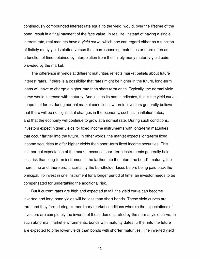
The difference in yields at different maturities reflects market beliefs about future

interest rates. If there is a possibility that rates might be higher in the future, long-term

loans will have to charge a higher rate than short-term ones. Typically, the normal yield

curve would increase with maturity. And just as its name indicates, this is the yield curve

shape that forms during normal market conditions, wherein investors generally believe

that there will be no significant changes in the economy, such as in inflation rates,

and that the economy will continue to grow at a normal rate. During such conditions,

investors expect higher yields for fixed income instruments with long-term maturities

that occur farther into the future. In other words, the market expects long-term fixed

income securities to offer higher yields than short-term fixed income securities. This

is a normal expectation of the market because short-term instruments generally hold

less risk than long-term instruments; the farther into the future the bond’s maturity, the

more time and, therefore, uncertainty the bondholder faces before being paid back the

principal. To invest in one instrument for a longer period of time, an investor needs to be

compensated for undertaking the additional risk.

But if current rates are high and expected to fall, the yield curve can become

inverted and long bond yields will be less than short bonds. These yield curves are

rare, and they form during extraordinary market conditions wherein the expectations of

investors are completely the inverse of those demonstrated by the normal yield curve. In

such abnormal market environments, bonds with maturity dates further into the future

are expected to offer lower yields than bonds with shorter maturities. The inverted yield

12

curve indicates that the market currently expects interest rates to decline as time moves

farther into the future, which in turn means the market expects yields of long-term bonds

to decline.

You may be wondering why investors would choose to purchase long-term

fixed-income investments when there is an inverted yield curve, which indicates that

investors expect to receive less compensation for taking on more risk. Some investors,

however, interpret an inverted curve as an indication that the economy will soon

experience a slowdown, which causes future interest rates to give even lower yields.

Before a slowdown, it is better to lock money into long-term investments at present

prevailing yields, because future yields will be even lower.

Figure 1-1. Normal yield curve Figure 1-2. Inverted yield curve

But the yield curve just give us an idea of the rate of borrowing for each term length.

It would be convenient if we could get the current, or instantaneous cost of borrowing in

a single number. What we can do is look at the current rate for instantaneous borrowing.

That is, borrowing which is paid back (nearly) instantly. Suppose at time t we borrow

over the period from t to t + �t, where �t is a small time increment, the rate we get is

the yield R(t, t + �t):

R(t, t + �t) = − logP(t, t + �t)

�t

13

As �t → 0, we call the limit the instantaneous rate, or short rate, rt , which is given by

both the expressions

rt = R(t, t),

and

rt = − ∂

∂TlogP(t, t).

The short rate is not only an important process in the interest rate market, but many

models are based exclusively on its behavior, with all the other bonds extrapolated from

it.

1.2 Models Of The Short-Term Interest Rate

The theory of interest-rate modeling was originally based on the assumption

of specific one-dimensional dynamics for the instantaneous rate process rt . Modeling

directly such dynamics is very convenient since all fundamental quantities (rates

and bonds) are readily defined as the expectation of a functional of the process rt .

The short term riskless interest rate is one of the most fundamental and important

prices determined in financial markets. More models have been put forward to explain

its behavior than for any other issue in finance. Many of the more popular models

currently used by academic researchers and practitioners have been developed in a

continuous-time setting, which provides a rich framework for specifying the dynamic

behavior of the short-term riskless rate. A partial listing of these interest rate models

includes those by Merton (1973) [38], Brennan and Schwartz (1982) [10], Vasicek

(1977) [42], Dothan (1978) [21], Cox, Ingersoll, and Ross (1985) [17], Hull and White

(1990) [29], Black, Fischer and Piotr Karasinski (1991) [8].

One of the earliest papers to tackle arbitrage-free pricing of bonds and interest-rate

derivatives was Vasicek (1977) [42]. This paper is best known for the Vasicek model for

the risk-free rate of interest, R(t) described below. However, Vasicek also developed

a more general approach to pricing which ties in with what we now refer to the as the

14

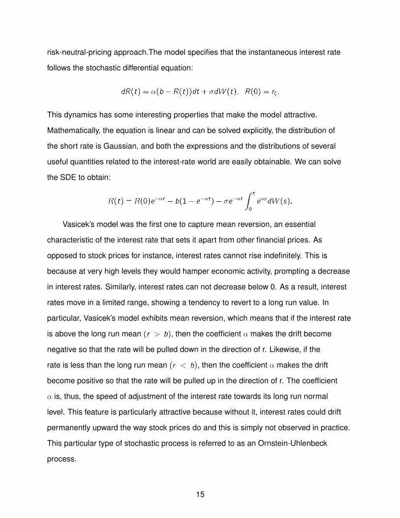
risk-neutral-pricing approach.The model specifies that the instantaneous interest rate

follows the stochastic differential equation:

dR(t) = α(b − R(t))dt + σdW (t), R(0) = r0.

This dynamics has some interesting properties that make the model attractive.

Mathematically, the equation is linear and can be solved explicitly, the distribution of

the short rate is Gaussian, and both the expressions and the distributions of several

useful quantities related to the interest-rate world are easily obtainable. We can solve

the SDE to obtain:

R(t) = R(0)e−αt + b(1− e−αt) + σe−αt

∫ t

0

eαsdW (s).

Vasicek’s model was the first one to capture mean reversion, an essential

characteristic of the interest rate that sets it apart from other financial prices. As

opposed to stock prices for instance, interest rates cannot rise indefinitely. This is

because at very high levels they would hamper economic activity, prompting a decrease

in interest rates. Similarly, interest rates can not decrease below 0. As a result, interest

rates move in a limited range, showing a tendency to revert to a long run value. In

particular, Vasicek’s model exhibits mean reversion, which means that if the interest rate

is above the long run mean (r > b), then the coefficient α makes the drift become

negative so that the rate will be pulled down in the direction of r. Likewise, if the

rate is less than the long run mean (r < b), then the coefficient α makes the drift

become positive so that the rate will be pulled up in the direction of r. The coefficient

α is, thus, the speed of adjustment of the interest rate towards its long run normal

level. This feature is particularly attractive because without it, interest rates could drift

permanently upward the way stock prices do and this is simply not observed in practice.

This particular type of stochastic process is referred to as an Ornstein-Uhlenbeck

process.

15

Figure 1-3. Three sample paths of different OU-processes with θ = 1,µ = 1.2,σ = 0.3

The main disadvantage is that, under Vasicek’s model, it is theoretically possible for

the interest rate to become negative, an undesirable feature. Since from the distribution

of R(t), it’s easy to see that R(t) is normally distributed with mean and variance given

by:

E(R(t)) = R(0)e−αt + b(1− e−αt)

Var(R(t)) =σ2

2α(1− e−2αt)

This implies that, for each time t, the rate R(t) can be negative with positive probability.

The general equilibrium approach developed by Cox, Ingersoll and Ross (1985) [17] led

to the introduction of a ”square-root” term in the diffusion coefficient of the instantaneous

short rate dynamics. The resulting model has been a benchmark for many years

because of its analytical tractability and the fact that, contrary to the Vasicek (1977) [42]

model, the instantaneous short rate is always positive. Hull and White (1990) [29]

proposed an even more general model by considering a time-varying parameter in

the Vasicek model. Later, Black and Karasinski (1991) [7] assumed that the logarithm

ln(R(t)) of the instantaneous short rate evolves according to a generalized Vasicek

16

model with time-dependent coefficients. In the next section, we’ll focus on the celebrated

CIR short rate model.

1.3 Introduction to CIR Model

The Cox-Ingersoll-Ross (CIR) [17] model is a diffusion process suitable for

modeling the term structure of interest rates. It was introduced in 1985 by John C. Cox,

Jonathan E. Ingersoll and Stephen A. Ross as an extension of the Vasicek model. The

simplest version of this model describes the dynamics of the interest rate X (t) as a

solution of the following stochastic differential equation (SDE):

dX (t) = α(b − X (t))dt + σ√X (t)dW (t), X (0) = x0 ≥ 0 (1–1)

for α > 0, b > 0,σ > 0 and a standard Brownian motion W. This process has some

appealing properties from an applied point of view, for example, the interest rate stays

non-negative, and is elastically pulled towards the long-term constant value b at a speed

controlled by α (mean-reverting). Those properties are attractive in modeling real-life

interest rates. In particular, the condition

2αb ≥ σ2

would ensure that the origin is inaccessible to the process, so that we can grant that

X (t) remains positive. Intuitively, when the rate is at a low level (close to zero), the

standard deviation σ√X (t) also becomes close to zero, which dampens the effect

of the random shock on the rate. Consequently, when the rate gets close to zero,

its evolution becomes dominated by the drift factor, which pushes the rate upwards

(towards equilibrium).

The interest rate behavior implied by this structure thus has the following empirically

relevant properties: (i) Negative interest rates are precluded. (ii) If the interest rate

reaches zero, it can subsequently become positive. (iii) The absolute variance of the

17

interest rate increases when the interest rate itself increases. (iv) There is a steady state

distribution for the interest rate.

Figure 1-4. An example of CIR process with α = 0.01, b = 1 and σ = 0.1

The SDE (1-1) is not explicitly solvable, hence the tractability of the CIR model is

not as good as the Vasicek model in this regard. Nevertheless, the transition density

for the process is known. Based on results of Feller [25], Cox et al. [17] noted that the

distribution of X (t) given X (u) for some u < t is, up to a scale factor, a non-central

chi-square distribution. In fact,

X (t)|X (u) ∼ cχ′d2(λ)

where

c =σ2(1− e−α(t−u))

4α, d =

4bα

σ2, λ =

4αe−α(t−u)

σ2(1− e−α(t−u))X (u).

Straightforward calculations give the expected value and variance of X (t) as:

E(X (t)|X (u)) = X (u)e−α(t−u) + b(1− e−α(t−u)),

Var(X (t)|X (u)) = X (u)(σ2

α)(e−α(t−u) − e−2α(t−u)) + b(

σ2

2α)(1− e−α(t−u))2.

18

Although CIR model is mainly used in finance in modeling interest rates, it should

be noted that this process has other financial applications. For example, the stochastic

volatility of the stock price (Heston) [27] and the credit spread (Brigo and Alfonsi) [11].

1.4 Simulation Issue

Financial models usually specify the dynamics of the state variables, e.g.,

stock price, volatility and interest rate, as stochastic differential equations (SDE). If these

SDEs yield closed form solutions, then Monte Carlo simulation can be used to generate

an unbiased estimator of the price of a derivative security. Basically we generate many

sample paths of the state variable and compute the payoff of the derivative for each

path. Discounting and averaging over all paths gives an estimator of the derivative price.

The error in the Monte Carlo estimator can be calculated using the central limit theorem

and converges to zero as the number of sample paths used increases.

However, in most cases, the SDEs that define the dynamics of the state variables

do not yield closed form solutions. In this case, it’s still possible to use Monte Carlo

simulation to compute derivative prices. But first we have to discretize the time interval

and simulating the state process dynamics on this discrete time grid. However, the

approximation of continuous time processes by discrete time processes introduces bias

into the simulation estimator.

One drawback of the CIR process is that the SDE (1-1) is not explicitly solvable.

In practical usage of such models (e.g. to price options) we are often faced with the

problem of simulating a CIR process. In general there are two ways to do it, namely,

exact simulation methods and approximation schemes. There are pros and cons

associated with each method. The drawback of exact simulation methods is the

computation time that they require. Exact simulation in general requires more time

than a simulation with approximation schemes (Up to a factor 10). Hence it should

be used to compute expectations that depend on the values of the process at just a

few fixed times. On the contrary, for expectations that depends on all the path (such

19

as integrals) discretization schemes should be preferred. On the other hand, the

drawback of approximation schemes in general is the bias they introduced into the

estimator. Since the magnitude of the bias is unknown, it’s difficult to obtain valid

confidence intervals. And another serious problem with discretization schemes of CIR

process, in general any square-root diffusion process, is the square-root itself, which has

unbounded derivatives near zero. Therefore, discretization schemes that (explicitly or

implicitly) involve the derivatives of the coefficients-even when they assure the positivity

of approximation-usually lose their accuracy near zero, especially, for large σ. The larger

σ is, the more concentrated near zero the value distributions of CIR process are. There

are ways to get around this problem, we’ll talk about them in detail in Chapter 2.

The first method is the exact simulation method, which is based on the transition

probability density function of the CIR process. In Cox’s paper [17], it was noted that the

distribution of X (t) given X (u) for any 0 < u < t is a noncentral chi-squared distribution.

The transition law of X (t) can be expressed as:

X (t)|X (u) ∼ cχ′d2(λ) (1–2)

where

c =σ2(1− e−α(t−u))

4α, d =

4bα

σ2, λ =

4αe−α(t−u)

σ2(1− e−α(t−u))X (u). (1–3)

This says that, given X (u), X (t) is distributed as σ2(1−e−α(t−u))/(4α) times a noncentral

chi-square random variable with d degrees of freedom and non-centrality parameter λ.

Thus, we can sample from the distribution of X (t) exactly, provided that we can

sample from the noncentral chi-square distribution. However, the drawback of the

traditional method in drawing non-central chi-square distribution is that it’s slow,

especially in the case when d < 1 and λ is relatively big. The exact reason will be

analyzed in chapter 3, but when the realization of the process along a lot of discrete

time is desired, the old exact simulation method is not efficient. It’s only competitive

20

when one has to simulate the process just at one time(or few times), for example to

compute European options prices with a Monte-Carlo algorithm. On the contrary, they

are drastically too slow if one has to simulate along a time-grid, as it is the case to

calculate path-dependent options prices.

The second one is the popular Euler discretization. Euler scheme can always

be used to approximate the paths of the interest rate process on a discrete time grid.

And it’s in general faster than the exact simulation, which will be mentioned later. The

drawback is that it’s an approximation of continuous time process by discrete time

process, hence introduces bias into the simulation estimator. And in practice, many time

steps may be necessary to reduce the bias to an acceptable level. Another problem is

that when discretizing a CIR process, or in general a square-root diffusion process, a

simple Euler scheme may not be well-defined because it can lead to negative values for

which the square root is not defined. Consider the following most straightforward Euler

scheme on the time interval [0,T ] for a CIR process X (t):

X (ti+1) = X (ti) + α(b − X (ti))[ti+1 − ti ] + σ

√X (ti)(W (ti+1)−W (ti))

with X (t0) = x0 > 0,α > 0, b > 0,σ > 0 can lead to negative values since the Gaussian

increment is not bounded from below. Thus, this simple scheme is not well defined.

To correct this problem, Deelstra and Delbaen [19] have proposed the ”full truncation

scheme”:

X (ti+1) = X (ti) + α(b − X (ti)+)[ti+1 − ti ] + σ

√X (ti)+(W (ti+1)−W (ti))

while Diop proposed in [6] proposed the ”reflection scheme”:

X (ti+1) = |X (ti) + α(b − X (ti))[ti+1 − ti ] + σ

√X (ti)(W (ti+1)−W (ti))|

21

Also, Alfonsi [1] [2] [3] presented several implicit schemes and higher order schemes.

In the next chapter, we’ll briefly review some basic properties of Euler scheme, and the

problems with simulating an CIR process with Euler schemes.

22

CHAPTER 2EULER EISCRETIZATION AND RELATED ISSUES

This section presents the simplest approximation, Euler scheme, to a

continuous-time stochastic process. This method is always easy to implement and

almost applicable everywhere, but it’s not always accurate enough to meet practical

needs. Most of the following introduction comes from Glasserman’s book [26].

2.1 Introduction To Euler-Maruyama Scheme

The Euler-Maruyama Scheme is a method for the approximate numerical

solution of a stochastic differential equation (SDE). It is a simple generalization of the

Euler method for ordinary differential equations to stochastic differential equations. We

consider a process X satisfying a stochastic differential equation of the form

dX (t) = a(X (t))dt + b(X (t))dW (t) (2–1)

with initial condition X (0) = x0, some fixed real number. We won’t get into details about

the uniqueness and existence conditions of the SDE, but essentially the coefficient

functions a and b are assumed to satisfy some technical conditions. Given the functions

a and b, the stochastic process X (t) is a solution of the SDE (2-1) if X (t) solves the

integral equation

X (t)− X (0) =

∫ t

0

a(X (s))ds +

∫ t

0

b(X (s))dW (s)

A famous example is the so called geometric Brownian motion, which is used to

model the evolution of asset prices. It’s a process satisfying the following SDE:

dS(t) = µS(t)dt + σS(t)dW (t)

We can actually solve this equation and get S(t) = S(0) exp{σW (t) + (µ− 12σ2)t}.

23

In practice, however, many SDE’s are not explicitly solvable like the above one.

Hence we can’t always get an analytical solution X (t) to a given SDE. But we could

always get approximate numerical solution of the given SDE. The basic idea is

essentially from Euler Scheme for ordinary differential equation (ODE). In particular,

let’s use X (t) to denote a time-discretized approximation to X (t). Suppose we discretize

the interval [0,T ]: let �t = T/N and tn = n�t, n = 0, 1, 2, ...,N. The exact solution on

the time grid would be

X (tn+1) = X (tn) +

∫ tn+1

tn

a(X (s))ds +

∫ tn+1

tn

b(X (s))dW (s)

The Euler-Maruyama approximation on the time grid 0 = t0 < t1 < ... < tN = T is

defined by

X (ti+1) = X (ti) + a(X (ti))[ti+1 − ti ] + b(X (ti))√ti+1 − tiZi+1,

with Z1,Z2, ... independent, m-dimensional standard normal random vectors. It is

a simple generalization of the Euler method for ordinary differential equations to

stochastic differential equations. It is named after Leonhard Euler and Gisiro Maruyama.

Implementation of this method is straightforward, when the functions a and b are

easy to evaluate. It’s easy to see that as the time grid gets finer, the Euler-Maruyama

approximation X (t) would converge to the real solution X (t). In the next section we’ll

talk about the convergence of Euler-Maruyama Scheme.

2.2 Convergence Order

Two broad categories of error of approximation are commonly used in

measuring the quality of discretization methods: criteria based on the path-wise

proximity of a discretized process to a continuous process, and criteria based on the

proximity of the corresponding distributions. These are generally termed strong and

weak criterion, respectively.

24

Definition (Strong error criterion) Given a sequence of discrete time approximation

{X (0), X (h), X (2h), ...} to a continuous time process X , where h = T/n for a fixed time

T . We say X converges strongly to X if it converges in L1, i.e., if

limn→∞

E(|X (nh)− X (T )|) = 0

We say that a discretization X has strong order of convergence γ > 0 if

E∥X (nh)− X (T )∥ ≤ chγ

for some vector norm ∥.∥, some constant c and for h sufficiently small.

The strong error criterion measures the deviation between the individual values of X

and the approximation X . In contrast, a weak error criterion looks like the following:

Definition (Weak error criterion) Given a sequence of discrete time approximation

{X (0), X (h), X (2h), ...} to a continuous time process X , where h = T/n for a fixed time

T . We say X converges weakly to X if

limn→∞

E(f (X (nh))) = E(f (X (T )))

We say that a discretization X has weak order of convergence γ > 0 if

|E(f (X (nh)))− E(f (X (T )))| ≤ chγ

for some constant c and for h sufficiently small, for all f whose derivatives of order

0, 1, ..., 2γ + 2 are polynomially bounded. (A function g is polynomially bounded if

|g(x)| ≤ k(1 + |x |q) for some constants k and q and all x ∈ R)

For applications in derivatives pricing, we really only care about the weak error

criteria. We would like to ensure that option prices (which are expectations) computed

from X (t) are close to prices computed from X (t). We are not really concerned about

the specific paths of the two processes.

25

Under modest conditions, even the simple Euler scheme converges as the time

step h decreases to zero. We compare different discretization schemes based on the

rate at which they converge. A large value of γ implies faster convergence to zero of

the discretization error. It’s often the case that for the same scheme, the strong order

of convergence is smaller than the weak order of convergence. For example, the Euler

scheme typically have a strong order of 1/2, but it often achieves a weak order of 1.

Stronger conditions are required for the Euler scheme to have weak order 1. In [34]

the authors require the functions a and b be four times continuously differentiable with

polynomially bounded derivatives. But good accuracy on smooth functions may not

be directly relevant to our intended applications: the CIR process has a square root

function, which is not Lipschitzian. This posed a problem for the ordinary Euler scheme.

We’ll discuss about this problem in the next section.

2.3 Euler Scheme For CIR Process

Using an Euler discretization to simulate CIR process gives rise to the

problem that while the process itself is guaranteed to be nonnegative, the discretization

is not. The main difficulty when discretizing the CIR process is located at 0, where the

square-root is not Lipschitzian. General schemes, such as the Euler scheme or the

Milstein scheme are in general not well defined because they can lead to negative

values for which the square root is not defined.

In Istvan and Miklos (2011) [30] the authors established the result of a convergence

speed estimate for Euler schemes corresponding to SDEs with 1/2-Holder continuous

diffusion coefficients. This result could be applied to CIR process, since the diffusion

coefficient of CIR process fails to be Lipschitz continuous near the origin. Hence

classical results on the rate of strong convergence for the corresponding Euler scheme

do not apply in this case. In general, they showed that the convergence rate for Euler

schemes corresponding to SDEs with 1/2-Holder continuous diffusion coefficients

26

(CIR as a special case) without any restrictions on the parameters should be 1/ ln n. In

particular, fix T > 0 and consider the SDE

dX (t) = b(t,X (t))dt + σ(t,X (t))dW (t), X (0) = ξ

on the interval [0,T ], where W (t) is a standard Brownian motion, ξ is independent of

W (t), and the coefficients satisfy the following conditions:

Assumption: σ, f , g : [0,T ] × R → R are measurable; g(t, ) is monotone

decreasing; b = f + g and there exist K > 0,α ∈ [0, 1/2] and γ ∈ (0, 1] such that for all

t ∈ [0,T ] and x, y∈ ℜ,

|σ(t, x)− σ(t, y)| ≤ K |x − y |1

2+α, |f (t, x)− f (t, y)| ≤ K |x − y |,

|g(t, x)− g(t, y)| ≤ K |x − y |γ,

and

|b(t, 0)|+ |σ(t, 0)| ≤ K .

Under the above assumption, the following theorem gives the convergence order of

Euler Scheme:

Theorem: Let the assumption above hold and let E |ξ|1+2α < ∞. Then there is a

constant C depending only on K ,T , γ and E |ξ|1+2α such that

E |X (τ)− Xn(τ)| ≤C

ln n, if α = 0.

E |X (τ)− Xn(τ)| ≤ C(1

nα+

1

nγ/2), if α ∈ (0,

1

2].

for all n ≥ 2 and for every stopping time τ ≤ T .

Hence for CIR process, which is the case when α = 0, without any restriction on the

parameters, a slow rate of O(1/ ln n) is established.

27

Also in Alfonsi’s paper [1] the author proposed several implicit discretization

schemes for the CIR process. But for large values of σ, for example, when σ2 >> 4αb,

none of the scheme seems to be efficient due to large discretization bias. In the next

chapter, we’ll look at a new method to simulate an CIR process exactly. The method is

exact, hence there is no discretization errors.

28

CHAPTER 3CIR PROCESS EXACT SIMULATION

In this section, we introduce the traditional exact simulation method of a CIR

process, and show why the so called ”Poisson method” is not efficient in some cases.

And we find a new method to simulate a non-central chi-squared random variable, which

is much more efficient than the Poisson method.

3.1 Traditional Simulation Method

The CIR process is a Markov process with continuous paths defined by the

following stochastic differential equation (SDE):

dX (t) = α(b − X (t))dt + σ√X (t)dW (t), X (0) = x0 ≥ 0

for α > 0, b > 0,σ > 0 and a standard Brownian motion W. As already mentioned

in chapter 1, the CIR process has some appealing properties and was originally used

to model interest rate in finance. It’s well known that there is a way to get the exact

distribution of the CIR process X (t), given X (u) for u < t. In fact, the transition law of

X (t) is a non-central chi-square distribution:

X (t)|X (u) ∼ cχ′d2(λ)

with degrees of freedom d =4bα

σ2, c =

σ2(1− e−α(t−u))

4αand non-centrality parameter

λ =4αe−α(t−u)

σ2(1− e−α(t−u))X (u). Hence, if we can sample from the non-central chi-squared

distribution, we can sample from the distribution of X (t) exactly.

Let’s first introduce some basic facts about central chi-square and non-central

chi-square distributions. If d is a positive integer and Z1, ...,Zd are independent N(0, 1)

random variables, then the distribution of Z 21 + Z 2

2 + ... + Z 2d is called the (central)

chi-square distribution with d degrees of freedom. The central chi-square random

variable is just a special case of a non-central chi-square random variable, with centrality

29

parameter 0. The symbol χ2d(0) denotes a random variable with this distribution;

the prime in χ′d2(λ) emphasizes that this symbol refers to the noncentral case. The

cumulative density function(CDF) of a central chi-square distribution is given by

P(χ2d(0) ≤ x) =

1

2d/2�(d/2)

∫ x

0

e−z/2z (d/2)−1dz ,

where �(.) denotes the gamma function �(z) =∫∞0

tz−1e−tdt and �(n) = (n − 1)! if n is

a positive integer. This expression defines a valid probability distribution for all d > 0 and

thus extends the definition of χ2d(0) to non-integer d .

For integer d and constants a1, ..., ad , the distribution of

d∑i=1

(Zi + ai)2 (3–1)

is noncentral chi-square with d degrees of freedom and non-centrality parameter

λ =∑d

i=1 a2i . Let χ′

d2(λ) denote a non-central chi-squared random variable with d

degrees of freedom and non-centrality parameter λ. The probability density function

(pdf) of this random variable is

g(λ, d , x) = e−λ2

∞∑j=0

(λ2)j

j!

e−x

2

�(d2+ j)

xd

2+j−1

2d

2+j

. (3–2)

and its characteristic function (c.f.) is

E exp{itχ′d2(λ)} = (1− 2it)−

d

2 exp{ λ

1− i2t− λ

2}.

This easily implies its additivity, namely

χ′d1

2(λ1) + χ′d2

2(λ2)d= χ′2

d1+d2(λ1 + λ2).

for two independent noncentral chi-square random variables with degrees of freedoms

d1, d2 and noncentrality parameters λ1, λ2, respectively. Therefore, in particular, we have

χ′d2(λ)

d= χ′

12(λ) + χ2

d−1(0), for d > 1 (3–3)

30

Therefore, to generate χ′d2(λ), d > 1, we can generate χ2

d−1(0) and an independent

standard normal random variable Z and set

χ′d2(λ) = (Z +

√λ)2 + χ2

d−1(0). (3–4)

Thus, sampling from a noncentral chi-squared distribution is reduced to sampling from

an ordinary chi-squared and an independent normal when d > 1. And this method is in

general quite efficient.

But for any 0 < d < 1, we can not shift λ to a normal random variable Z. In this

case, a noncentral chi-squared random variable can only be generated as an ordinary

chi-squared random variable with a random degrees of freedom parameter. In order to

see this, suppose N is a Poisson random variable with mean λ/2, then

P(N = j) = e−λ/2 (λ/2)j

j!, j = 0, 1, 2, ...

Consider now a random variable χ2d+2N(0) with N having this Poisson distribution.

Conditional on N = j , the random variable has an ordinary (central) chi-square

distribution with d + 2j degrees of freedom:

P(χ2d+2N(0) ≤ x |N = j) =

1

2d/2+j�(d/2 + j)

∫ x

0

e−z/2z (d/2)+j−1dz ,

The unconditional distribution is thus given by

∞∑j=0

P(N = j)P(χ2d+2N(0) ≤ x |N = j) =

∞∑j=0

e−λ/2 (λ/2)j

j!P(χ2

d+2j(0) ≤ y),

which is precisely the non-central chi-square distribution with degrees of freedom d and

non-centrality parameter λ.

Therefore, we have the following relationship:

χ′d2(λ)

d= χ2

d+2N(0), for d < 1. (3–5)

31

We may therefore sample χ′d2(λ) by first generating a Poisson random variable N with

mean λ/2 and then, conditional on N, sampling a chi-square random variable with

d +2N degrees of freedom. This method can be used to sample χ′d2(λ) when 0 < d < 1,

and in general is reasonably fast. Theoretically, being able to generate a noncentral

chi-square random variable, we could generate a discrete time sample path of a CIR

process based on the conditional distribution X (t)|X (u). In other words, given an initial

X (0) and any time grid 0 = t0 < t1 < ... < tN = T , we are able to generate a non-biased

sample of the CIR process on the time grid.

But we’ll see in the next section that it can only be used if we just need to generate

one non-central chi-square random variable, with λ not very big. In real life, numerous

derivatives have a path-dependent feature. In other words, their prices usually depend

on the underlying asset not only at one single time point, but many of them. In this

case, we would have to simulate the CIR process along a time grid with many time

points. This is not a serious problem when CIR process is used to model interest rate,

since d would typically be larger than 2. But when applied to model variance process

in a stochastic volatility model, like Heston’s model, it poses serious problem since

σ is often much bigger than in the interest rate model. In this case, d =4bα

σ2would

typically be less than 1, and in many cases close to 0. This is exactly the situation

where the ”Poisson method” has to be used to generate a CIR process. Although the

above method yields sample with no bias, practitioners often have to settle for Euler

discretization methods to price path-dependent derivatives under Heston’s model,

since the above algorithm is too slow for real time simulation. We’ll analyze in detail

the reason why the traditional method to simulate a CIR process is not efficient in this

case to price path-dependent securities in the next section. More efficient algorithm to

generate CIR processes is needed in this situation.

32

3.2 Some Drawbacks In Simulating CIR Process

Let’s use the algorithm above to simulate a CIR process. In particular, we only

consider the case when d < 1, since that’s when we have to use the ”Poisson method”

for simulation. Suppose we want to simulate a CIR process X (t) along n equally spaced

time points on the time interval [0,T ]. In this case, given an initial value X (0), we

could use the transition distribution of X (t) to simulate a random vector distributed

according to the law of (X (T/n),X (2T/n), ...,X (T )) inductively. Let t0, t1, t2, ..., tn to

denote the time points 0,T/n, 2T/n, ...,T . Starting from X (0), which is given, we could

generate the whole sample path of the CIR process along the time grid ti iteratively.

In general, given X (ti−1), the conditional distribution of X (ti) is cχ′d2(λ(i)), where

c =σ2(1− e−α�t)

4α, λ(i) =

4αe−α�t

σ2(1− e−α�t)X (ti−1). Here �t = ti − ti−1 = T

n. It’s easy to

see that the value of λ(i) depends on X (ti−1) and �t. This fact turns out to be the major

problem in simulating a CIR process with d < 1 using the Poisson method along many

time points.

Suppose we want to use Monte Carlo method to approximate a path-dependent

option (for example, Asian option or Lookback option), assuming the underlying asset

price process follows the Heston stochastic volatility model. In particular, the payoff

function of a standard European-style discrete Asian call option is

(1

n + 1

n∑i=0

Sti − K)+

whereas the payoff function of a fixed strike discrete Lookback call option is

(max0≤i≤n

Sti − K)+

Here St denotes the underlying asset price at time t, K is the strike price. A typical

Monte Carlo method involves simulating the asset price on the time grid 0 = t0 < t1 <

... < tn = T for M times, where M is typically much bigger compared with the number of

time points n. For each sample of the asset price process, compute the corresponding

33

payoff function value. Then the Monte Carlo estimation of the option price is given by the

mean value of the discounted payoff values along those different paths generated.

Thus, in order to compute the price of a path-dependent option using Monte Carlo

method, we are interested in simulating an asset price process along a lot of time points.

In particular, Heston’s model use a CIR process to model the evolution of stochastic

volatility. Hence in order to simulate the asset price process, we first need to simulate a

CIR process along those time points. As mentioned above, the fact that the value of λ(i)

depends on X (ti−1) and �t poses a problem in simulating the CIR process. The reason

is that when the needed number of time points n is big, �t = T/n is very small. In this

case λ(i) =4αe−α�t

σ2(1− e−α�t)X (ti−1) would be huge since it’s a decreasing function of �t,

and actually goes to ∞ as �t → 0. This poses a serious problem for the simulation.

Because when d < 1, which is common for Heston model, in order to generate a

non-central chi-square random variable χ′d2(λ(i)), we need to first generate a Poisson

random variable with mean λ(i)/2. Then conditional on the value of the Poisson random

variable N, generate a central chi-square random variable χ2d+2N(0). Normally, in order

to calculate the price of a path-dependent option, the number of time points we need

is big. In this case the algorithm will spend a huge amount of time generating Poisson

random variables at each time point, since λ(i)/2 is huge. Hence, although theoretically

this algorithm could still be used to simulate a CIR process at multiple time points, it’s

not efficient if the number of time points involved is big. In this case people prefer to use

Euler Scheme to generate the sample path instead, although it often generate results

which are biased and not accurate. Because the Poisson method is simply too slow.

In the next section, we’ll introduce a new method to generate a non-central chi-square

random variable, which avoids this problem.

34

3.3 Main Result

The following theorem provides a new method to generate a non-central chi

square random variable based on a central chi square random variable.

Theorem A noncentral Chi-square r.v χ2d(λ) can be expressed by

χ2d(λ)

d= χ2

d(0) + Y(λ,Z , ~Z ,U) (3–6)

where χ2d(0) has a gamma distribution G(d/2, 2), U has a uniform distribution on

[0, 1], Z and ~Z are standard normal random variables. All four random variables are

independent, and

Y(λ,Z , ~Z ,U) =

0, : if λ+ 2 ln(U) ≤ 0.

(Z +√

λ+ 2 ln(U))2 + ~Z 2, : if λ+ 2 ln(U) > 0.(3–7)

Proof: The probability density function g(λ, d , x) of χ2d(λ) is given by

g(λ, d , x) = e−λ2

∞∑j=0

(λ2)j

j!

e−x

2

�(d2+ j)

xd

2+j−1

2d

2+j

.

from this density function, we have

eλ2 g(λ, d , x) = g(0, d , x) +

∞∑j=1

(λ2)j

j!

e−x

2

�(d2+ j)

xd

2+j−1

2d

2+j

.

where g(0, d , x) =e−

x

2

�(d2)

xd

2−1

2d

2

is the density function of χ2d(0). Now, differentiating both

sides w.r.t λ yields

∂

∂λ(e

λ2 g(λ, d , x)) =

1

2

∞∑j=1

(λ/2)j−1

(j − 1)!g(0, d + 2j , x)

=1

2

∞∑j=0

(λ/2)j

j!g(0, d + 2 + 2j , x)

=1

2e

λ2 g(λ, d + 2, x).

35

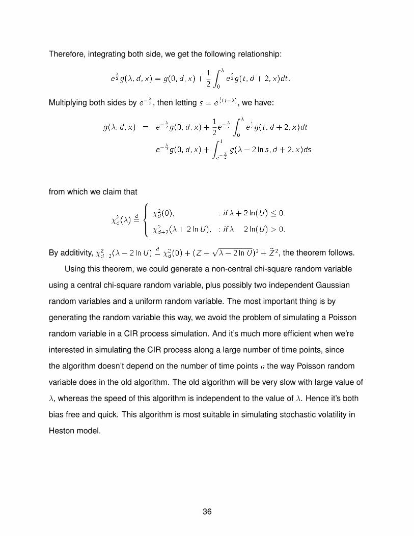
Therefore, integrating both side, we get the following relationship:

eλ2 g(λ, d , x) = g(0, d , x) +

1

2

∫ λ

0

et

2g(t, d + 2, x)dt.

Multiplying both sides by e−λ2 , then letting s = e

1

2(t−λ), we have:

g(λ, d , x) = e−λ2 g(0, d , x) +

1

2e−

λ2

∫ λ

0

et

2g(t, d + 2, x)dt

= e−λ2 g(0, d , x) +

∫ 1

e−λ

2

g(λ+ 2 ln s, d + 2, x)ds

from which we claim that

χ2d(λ)

d=

χ2d(0), : if λ+ 2 ln(U) ≤ 0.

χ2d+2(λ+ 2 lnU), : if λ+ 2 ln(U) > 0.

By additivity, χ2d+2(λ+ 2 lnU)

d= χ2

d(0) + (Z +√λ+ 2 lnU)2 + ~Z 2, the theorem follows.

Using this theorem, we could generate a non-central chi-square random variable

using a central chi-square random variable, plus possibly two independent Gaussian

random variables and a uniform random variable. The most important thing is by

generating the random variable this way, we avoid the problem of simulating a Poisson

random variable in a CIR process simulation. And it’s much more efficient when we’re

interested in simulating the CIR process along a large number of time points, since

the algorithm doesn’t depend on the number of time points n the way Poisson random

variable does in the old algorithm. The old algorithm will be very slow with large value of

λ, whereas the speed of this algorithm is independent to the value of λ. Hence it’s both

bias free and quick. This algorithm is most suitable in simulating stochastic volatility in

Heston model.

36

CHAPTER 4INTRODUCTION TO HESTON MODEL AND SIMULATION

This chapter briefly discusses basic option pricing theory. In particular,

Heston’s stochastic volatility (SV) model is introduced and how the exact simulation

method can be used to price options.

4.1 Option Pricing Theory

Options have existed for a long time. It wasn’t until publication of the Black-Scholes

(1973) [9] option pricing formula that a theoretically consistent framework for pricing

options became available. That framework was a direct result of work by Robert Merton

as well as Black and Scholes. Since then the derivatives market has grown into a

multi-trillion dollar industry. Options have become important to industry, particularly as

they can be used to hedge out risk. Option pricing in itself has become an important

research area. Numerous option pricing models were proposed, each one trying to

generalize the Black-Sholes framework by relaxing one or more of the unrealistic

restrictions of the original Black-Sholes model.

An Option is a major financial derivative, it gives the holder of that option the right,

not the obligation to trade a fixed amount of underling asset at an agreed-upon price

on the maturity date (European option) or any time on or before the maturity date

(American option). A call option gives the holder the right, but not obligation to buy, a

put option gives the holder the right, but not obligation to sell. There are two sides of

every option contract. On one side is the investor who has taken the long position(i.e.,

has bought the option). On the other side is the investor who has taken a short position

(i.e., has sold or written the option). The most straight forward financial derivatives are

European call option and European put option. The price in the contract is known as

the strike price; the date in the contract is known as the maturity. The payoff from a long

37

position in a European call option is:

max(S(T )− K , 0)

where T is the maturity, S(T ) is the stock price at maturity, and K is the strike price.

Hence, the buyer of a European call option hopes the price of the underlying stock

would rise above K at the maturity, in which case he would use the right to buy the stock

at K and make a profit. But if the stock price would drop below K at maturity, he doesn’t

have the obligation to exercise the option. Similarly, the payoff from a long position in a

European put option is:

max(K − S(T ), 0)

Although it’s fairly easy to understand the payoff structure of different types of options, to

price them is quite a different story. The question of how options should be priced had

been the subject of long intellectual debates, starting from the early sixties.

Option pricing theory traces its root to Bachelier (1900) who used Brownian motion

to model options on French government bonds. This work anticipated by five years

Einstein’s independent use of Brownian motion in physics. Somehow, the research

didn’t pick up until 1960’s. In Samuelson (1965) [39], he considered long-term equity

options, and used geometric Brownian motion to model the random behavior of the

underlying stock. Based upon this, he modeled the random value of the option at

exercise. Unfortunately, Samuelson’s formula was largely arbitrary. It offered no means

for a buyer and seller with different risk aversions to agree on a price for an option.

In the seminal paper by Black and Scholes (1973) [9], they derived a partial

differential equation for valuing claims contingent on a traded underlying asset. The

equation is general. By applying different boundary conditions, it can be solved to price

any such contingent claim. Black and Scholes applied the boundary conditions for a

European call option on a non-dividend-paying stock and obtained their famous option

pricing formula. The key idea behind the derivation was to perfectly hedge the option by

38

buying and selling the underlying asset in just the right way and consequently ”eliminate

risk”. This hedge is called delta hedging and is the basis of more complicated hedging

strategies.

In the original Black-Scholes model, they assumed that the derivative’s underlying

price follows a standard model for geometric Brownian motion:

dS(t) = µS(t)dt + σS(t)dWt

where µ is a constant drift(expected return) of the security price S(t), σ is the constant

volatility, and Wt is a standard Brownian motion. This stochastic differential equation(SDE)

has the following explicit solution:

S(t) = S(0)e(µ−1

2σ2)t+σWt

Under those assumptions, they derived a partial differential equation, now called

the Black-Scholes equation, which governs the price of the option over time. The key

idea behind the derivation was to perfectly hedge the option by buying and selling the

underlying asset in just the right way and consequently ”eliminate risk”. Suppose we

construct the following portfolio:

� = V (S ,T )− �S

Here V (S ,T ) denotes a value of one long option position and � is the amount short in

the underlying. The value of the hedged portfolio will change by

d� = dV (S ,T )− �dS

Using Ito’s formula, we have

dV =∂V

∂tdt +

∂V

∂SdS +

1

2σ2S2∂

2V

∂S2dt

39

Plug in, the change in the portfolio will be:

d� = (∂V

∂t+

1

2σ2S2∂

2V

∂S2)dt + (

∂V

∂S− �)dS

Hence, The risk in the portfolio � is removed if

∂V

∂S− � = 0

Therefore, the quantity � is chosen as

� =∂V

∂S

If the portfolio is delta hedged continuously (dynamic hedging strategy), then a risk-less

portfolio is constructed with a dynamics given by

d� = (∂V

∂t+

1

2σ2S2∂

2V

∂S2)dt

Since there is no stochastic term, � is a risk-free investment and hence must offer

the same return as any other risk-free investment. Therefore, from the no-arbitrage

condition

d� = r�dt

It is important to note that the portfolio � represents a self-financing, replicating and

hedging strategy. It replicates a risk-free investment and it is hedged since it has no

stochastic component. Making substitutions to equation it is obtained that

(∂V

∂t+

1

2σ2S2∂

2V

∂S2)dt = r(V − S

∂V

∂S)dt

Simplifying the above equation, we showed that the payoff of any contingency claim

V (s, t) must satisfy the following partial differential equation(Black-Scholes equation):

∂V

∂t+

1

2σ2S2∂

2V

∂S2+ rS

∂V

∂S= rV

40

Coupled with the appropriate terminal and boundary conditions, they got closed-form

solutions for European call and put options. The value of a call option for a non-dividend

paying underlying stock in terms of the Black-Scholes parameters is:

C(S , t) = N(d1)S − N(d2)Ke−r(T−t)

d1 =log S

K+ (r + σ2

2)(T − t)

σ√T − t

d2 =log S

K+ (r − σ2

2)(T − t)

σ√T − t

= d1 − σ√T − t

The price of a corresponding put option is:

P(S , t) = N(−d2)Ke−r(T−t) − N(−d1)S

where N(.) is the cumulative density function of the standard normal distribution, T − t

is the time to maturity, S is the spot price of the underlying asset, K is the strike price, r

is the risk free rate, and σ is the volatility of returns of the underlying asset.

Alternatively, there is another way to find the price of derivatives, namely risk

neutral pricing. This is one of the most important principles in derivative valuation. Risk

neutral pricing is a powerful method for computing prices of derivative securities. The

basic idea of risk neutral pricing is that given a realistic market model for the stock

price process, we can construct a ”risk free” portfolio that consists only the underlying

stock and risk free bond. If there exists an equivalent measure Q under which the

discounted stock price process is a martingale (the risk-neutral measure), then based

on Martingale Representation Theorem, we could perfectly replicate any contingency

claim based on the stock. The real world probability measure P, surprisingly, has

nothing to do with option pricing. Finding this particular equivalent measure Q relies on

Girsanov theorem. After we get this perfect replicating scheme, it’s easy to argue, based

on no arbitrage pricing theory, that the only arbitrage-free price of the claim at time

zero is the expected value of the discounted payoff of the claim under the risk-neutral

41

measure Q. In particular, for an European call option, the payoff at maturity T is given

by (S(T ) − K)+, where K is the strike price. Hence, risk-neutral pricing tells us that the

price of the European call at time 0 is:

EQ[e−rT (S(T )− K)+]

Since Black and Scholes published their seminal article on option pricing in 1973,

there has been vast explosions of theoretical and empirical investigation on option

pricing. People start to realize that the Black-Scholes model disagrees with reality in a

number of ways, some significant. For example, empirical studies have shown that an

asset’s log-return distribution is non-Gaussian. It is characterized by heavy tails and

high peaks (leptokurtic). There is also empirical evidence and economic arguments that

suggest that equity returns and implied volatility are negatively correlated (also termed

the leverage effect). This departure from normality plagues the Black-Scholes-Merton

model with many problems. Another problem is that the Black-Scholes model assumes

constant volatility. If the Black-Scholes model held, then the implied volatility for a

particular stock would be the same for all strikes and maturities. In practice, the volatility

surface (the three-dimensional graph of implied volatility against strike and maturity) is

not flat. The typical shape of the implied volatility curve for a given maturity depends

on the underlying instrument. This is the famous ”volatility smile effects”, which is

a long-observed pattern in which at-the-money options tend to have lower implied

volatilities than in- or out-of-the-money options. Finally, Black-Scholes model assumes

continuous paths of the stock price, whereas in real life, jumps in equity prices frequently

happen.

In the last two decades, option pricing has witnessed an explosion of new models

that each relax some of the restrictive Black-Scholes (BS) (1973) assumptions.

Examples include:

42

(i) the stochastic-interest-rate option models of Merton (1973) [38] and Amin and

Jarrow (1992) [33];

(ii) the jump-diffusion/pure jump models of Bates (1991) [18], Madan and Chang

(1996) [20], and Merton (1976) [37];

(iii) the constant-elasticity-of-variance (CEV) model of Cox and Ross (1976) [31];

(iv) the stochastic volatility models of Heston (1993) [27], Hull and White (1987a) [28],

Melino and Turnbull (1990) [36], Scott (1987) [41], Stein and Stein (1991) [23], and

Wiggins (1987) [43];

(v) general Levy models of Bandorff-Nielsen, O. (1998) [5], Eberlein, E., U. Keller

and K. Prause (1998) [22], Carr, P., H. Geman, D.B. Madan and M. Yor (2002) [13], Carr,

P. and L, Wu (2003) [15].

In the next section, we’ll focus on one of the approaches above, namely, stochastic

volatility models.

4.2 Introduction To Stochastic Volatility Model

The volatility of a financial asset is defined as the standard deviation per unit of time

of the continuously compounded asset returns. It is an important input to many financial

decisions such as asset allocation, option pricing, and risk management.

Stochastic volatility models are one approach to resolve a shortcoming of the

Black-Scholes model. In particular, Black-Scholes model assumes that the underlying

volatility is constant over the life of the derivative, and unaffected by the changes in the

price level of the underlying security. The observed market returns display non constant

volatility, clustering and are not normal distributed. The implied volatility is the volatility of

the underlying which, when substituted into Black-Scholes formula, gives a theoretical

price equal to the market price. The implied volatilities of options in the market show

dependence on strike and time to expiration and are not constant. If the Black-Scholes

43

model is correct, then all options on the same underlying asset should give the same

implied volatility. However, Black-Scholes implied volatilities usually vary across strike

prices and across maturities. Taking limitations of Black-Scholes into account, one might

see the apparent benefits of using non-constant volatility models.

One of the appealing features of the Black-Scholes model is that it yields closed-form

analytic formulaes for many different kinds of options. It assumes a constant volatility,

which is unobservable in the market. In practice, people often use implied volatility to

measure option’s relative value. Implied volatility is the volatility that, when used in a

particular pricing model, yields a theoretical value for the option equal to the current

market price of that option. Thus, if the assumption of constant volatility were right, the

implied volatility using Black-Scholes model should be the same across all possible

strikes and maturities. But extensive empirical evidences during the past decades have

shown that it’s not the case. In particular, from the following graph, it’s easy to see that

the implied volatility surface is far from flat.

Figure 4-1. Implied Volatility Surface

To model the stochastic evolution of volatility over time, an assumption about the

stochastic process that governs its dynamics needs to be made. The specification of

the process should be based on its ability to explain most of the empirical regularities

44

of volatility. Several empirical studies have investigated the time-series properties of

volatility. The main findings includes:

(i)Fat tails. Since the early sixties, many empirical studies have found that the

probability that extreme events will occur is greater than the corresponding probability

calculated under the normal distribution. In other words, the empirical distribution of

returns exhibits excess kurtosis; it accumulates more probability mass in the tails (i.e.,

”fat tails”) than the normal distribution does. This is called a leptokurtic distribution.

(ii)Mean Reversion in Volatility. Empirical studies have found that volatility oscillates

around a constant value. This phenomenon is termed ”mean reversion,” indicating that

volatility tends to revert to a long-run mean.

(iii)Leverage Effect. In 1976, Fischer Black noted that there is a negative relationship

between volatility and price changes. This phenomenon is termed ”leverage effect.”

Christie (1982) [16] attributed the leverage effect to the fact that a drop in stock prices

tends to increase the leverage of the firm, which in turns increases its risk as this is

measured by volatility.

(iv)Clustering Effect. Any casual observation of financial time series reveals clusters

of high and low volatility episodes. Mandelbrot (1963) [35] and Fama (1965) [24]

reported evidence that periods of high (low) volatility are followed by periods of high

(low) volatility. Mandelbrot has called this phenomenon ”the clustering effect” of volatility.

In either case, the sign of changes from one period to the next is unpredictable. Volatility

clustering suggests the presence of autocorrelation in volatility changes.

After the stock market crash in 1987, it was evident that volatility of the stock returns

could not be treated as a constant parameter. Hull and White’s model (1987) [28] was

one of the earliest and simplest stochastic volatility models that was introduced in

the same year the stock market crashed. In particular, they considered the following

dynamics:

dS(t) = µS(t)dt +√V (t)S(t)dW1(t)

45

dV (t) = aV (t)dt + bV (t)dW2(t)

where dW 1t dW

2t = ρdt, and a, b are positive constants. In this case, the volatility

σt =√V (t) is a geometric Brownian motion.

Scott (1989) [40] considered the case in which the logarithm of the volatility is a

mean reverting process and this was further developed by Stein and Stein (1991) [23].

He assumed the stock price follows:

dS(t) = µS(t)dt + exp(V (t))S(t)dW1(t)

dV (t) = a(b − V (t))dt + cdW2(t)

where dW1(t)dW2(t) = ρdt, and a, b and c are positive constants. In this case, the

log-volatility V (t) = log σ(t) is an Ornstein-Uhlenbeck (OU) process.

In 1993 Heston introduced a model where the volatility is related to a mean

reverting square root process, commonly known as CIR process. The mean reverting

square root process was first introduced by Cox, Ingersoll and Ross (1985) [17] to

imitate the behavior of risk-free interest rate. Heston offers a stochastic volatility model

that is not based on the BS formula. It provides a closed form solution for the price of a

European call option when the spot asset is correlated with volatility (Heston 1993) [27].

These features made the Heston model popular for pricing plain vanilla options. In the

next section we’ll introduce Heston’s model.

4.3 Introduction To Heston’s Model And Simulation Issue

Heston model (1993) is the most successful stochastic volatility model that

attempts to capture the smile effect observed in implied volatilities of liquidly traded

options, and to fulfill the gap of the unrealistic constant volatility assumed in the

Black-Scholes model [9]. In Heston model, variances, not volatilities, are specified

46

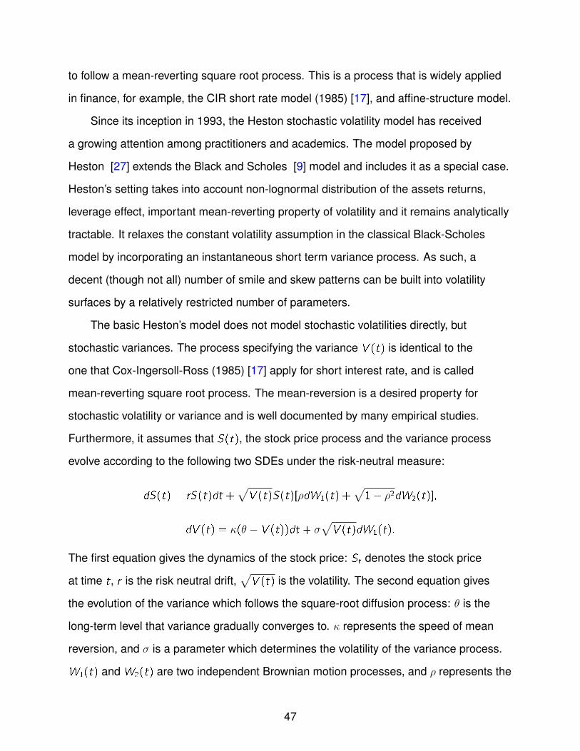
to follow a mean-reverting square root process. This is a process that is widely applied

in finance, for example, the CIR short rate model (1985) [17], and affine-structure model.

Since its inception in 1993, the Heston stochastic volatility model has received

a growing attention among practitioners and academics. The model proposed by

Heston [27] extends the Black and Scholes [9] model and includes it as a special case.

Heston’s setting takes into account non-lognormal distribution of the assets returns,

leverage effect, important mean-reverting property of volatility and it remains analytically

tractable. It relaxes the constant volatility assumption in the classical Black-Scholes

model by incorporating an instantaneous short term variance process. As such, a

decent (though not all) number of smile and skew patterns can be built into volatility

surfaces by a relatively restricted number of parameters.

The basic Heston’s model does not model stochastic volatilities directly, but

stochastic variances. The process specifying the variance V (t) is identical to the

one that Cox-Ingersoll-Ross (1985) [17] apply for short interest rate, and is called

mean-reverting square root process. The mean-reversion is a desired property for

stochastic volatility or variance and is well documented by many empirical studies.

Furthermore, it assumes that S(t), the stock price process and the variance process

evolve according to the following two SDEs under the risk-neutral measure:

dS(t) = rS(t)dt +√V (t)S(t)[ρdW1(t) +

√1− ρ2dW2(t)],

dV (t) = κ(θ − V (t))dt + σ√V (t)dW1(t).

The first equation gives the dynamics of the stock price: St denotes the stock price

at time t, r is the risk neutral drift,√V (t) is the volatility. The second equation gives

the evolution of the variance which follows the square-root diffusion process: θ is the

long-term level that variance gradually converges to. κ represents the speed of mean

reversion, and σ is a parameter which determines the volatility of the variance process.

W1(t) and W2(t) are two independent Brownian motion processes, and ρ represents the

47

instantaneous correlation between the return process and the volatility process. If the

parameters obey the condition 2κθ ≥ σ2 (known as the Feller condition) then the process

V (t) is strictly positive. Typically, the correlation ρ is negative, pointing to the fact that

a down-move in the stock price is correlated with an up-move in the volatility (leverage

effect).

It is worthwhile mentioning that the variance process V (t) is noncentrally chi-square

distributed. In fact,

V (t)|V (s) ∼ cχ′d2(λ)

where

c =σ2(1− e−κ(t−s))

4κ, d =

4κθ

σ2, λ =

4κe−κ(t−s)

σ2(1− e−κ(t−s))V (s).

Based on the properties of a non-central chi-square distribution, V (t) has the following

two conditional moments:

E(V (t)|V (s)) = θ + (V (s)− θ)e−κ(t−s),

Var(V (t)|V (s)) = V (s)(σ2

κ)(e−κ(t−s) − e−2κ(t−s)) + θ(

σ2

2κ)(1− e−κ(t−s))2.

If κ, θ and σ satisfy the following condition:

2κθ > σ2, V0 > 0,

it can be shown that variances V (t) are always positive and the variance process is then

well-defined under the above condition.

Heston is the first one who proposes a closed-form price for a standard European

call when using a square-root volatility process by inverting the characteristic function

seen as a Fourier transform. But there is no close-form price for path-dependent exotic

options, where the option payoff depends on the whole path of the underlying asset

price. Many practical applications of models with Heston-dynamics involve the pricing

48

and hedging of path-dependent options, which, in turn, nearly always requires the

introduction of Monte Carlo methods.

Given some arbitrary set of discrete times {ti}Ni=1, we want to generate random

paths of the pair (S(t),V (t)) along those discrete times. This would be required, for

instance, in the pricing of path-dependent securities with payout functions that depend

on observations of S(t) at a given finite set of dates. In order to do that, it suffices to be

able to generate (S(t + �),V (t + �)) given (S(t),V (t)). A few previously proposed

techniques for updating S(t) and V (t) from time t to time t +� include a ”full truncation”

scheme based on a naive Euler scheme, Kahl-Jackel discretization scheme involving

an implicit Milstein scheme for the V-process and their ”IJK” discretization for the stock

process, Broadie-Kaya scheme based on an exact distribution of S(t), and Anderson’s

QE scheme.

The naive Euler scheme with a ”full truncation” fix would take the following form:

ln S(t + �) = ln S(t) + (r − 1

2V (t)+)� +

√V (t)+(ρZ1 +

√1− ρ2Z2)

√�,

V (t +�) = V (t) + κ(θ − V (t)+)� + σ

√V (t)+Z1

√�

where Z1 and Z2 are independent standard Gaussian variables, and the notation

x+ = max(x , 0). Its main characteristic is that the process for V is allowed to go below

zero, at which point the process for V becomes deterministic with an upward drift of κθ.

The bias of the Monte Carlo estimator for the stock price using this naive Euler scheme

becomes really big when σ is relatively big and 2κθ << σ2.

Kahl-Jackel (2006) [32] suggests discretizing the V-process using an implicit

Milstein scheme, and coupled with their ”IJK” discretization for the stock process. They

proposed the following scheme:

ln S(t + �) = ln S + (r − 1

4(V (t + �) + V (t)))� + ρ

√V (t)Z1

√�

+1

2(

√V (t +�) +

√V (t))

√1− ρ2Z2

√� +

1

4σρ�(Z 2

1 − 1),

49

V (t + �) =V (t) + κθ� + σ

√V (t)Z1

√� + 1

4σ2�(Z 2

1 − 1)

1 + κ�

But one thing about this scheme is that it only results in positive paths for the V process

if 4κθ > σ2. In practice, this restriction is rarely satisfied. Thus this scheme for V

will produce negative values with substantial probability. To fix this, we use a similar

approach like the ”full truncation” Euler scheme. Basically whenever V (t) drops below

zero, we use the naive Euler scheme (deterministic with an upward drift of κθ) to get

V (t + �). Otherwise, use the above scheme for V (t) and make sure to use V (t + �)+

and V (t)+ in sampling ln S(t + �).

Broadie-Kaya (2006) [12] used the Poisson method to sample V (t + �) directly.

Basically, the scheme involves sampling from a Poisson distribution, and then sample

from a central chi-square distribution with its degree of freedom parameter determined

by the outcome of the Poisson draw. As we already mentioned in simulating CIR

process, this method of sampling a non-central chi square random variable with degrees

of freedom less than 1 is not efficient. After this, to obtain a bias-free scheme for

sampling the stock price process, first integrate the SDE for V (t), and get

V (t + �) = V (t) +

∫ t+�

t

κ(θ − V (u))du + σ

∫ t+�

t

√V (u)dW1(u)

or we could write it as∫ t+�

t

√V (u)dW1(u) = σ−1(V (t + �)− V (t)− κθ� + κ

∫ t+�

t

V (u)du).

Now, by Ito’s formula, the log-stock price satisfies the following SDE:

d lnS(t) = (r − 1

2V (t))dt + ρ

√V (u)dW1(u) +

√1− ρ2

√V (u)dW2(u)

In integral form, we have

lnS(t + �) = lnS(t) + r� +ρ

σ(V (t + �)− V (t)− κθ�)

50

+(κρ

σ− 1

2)

∫ t+�

t

V (u)du +√

1− ρ2∫ t+�

t

√V (u)dW2(u)

after plugging in the expression of∫ t+�

t

√V (u)dW1(u) from earlier. Since V (u) and

W2(u) are independent, the distribution of∫ t+�

t

√V (u)dW2(u) given the path generated

by V (t) is normal with mean 0 and variance∫ t+�

tV (u)du. Now it’s clear that conditional

on V (t + �) and∫ t+�

tV (u)du, the distribution of lnX (t + �) is Gaussian with easily

computable first and second moments. They examined the characteristic function of∫ t+�

tV (u)du and numerically Fourier-invert to get the distribution function, which is very

complicated numerically. As mentioned in Anderson’s paper, rather than using Fourier

methods, simply write

∫ t+�

t

V (u)du ≈ �[γ1V (t) + γ2V (t +�)]

for certain constants γ1 and γ2. There are multiple ways for setting γ1 and γ2, the

simplest being the Euler-like setting: γ1 = 1, γ2 = 0. Or a central discretization:

γ1 = γ2 =12.

We use our new method to simulate the path of V (t), and use the above approach

instead of Broadie and Kaya’s approach to approximate∫ t+�

tV (u)du. After plugging in

the approximation, we have:

ln S(t + �) = ln S(t) + r�+ρ

σ(V (t + �)− V (t)− κθ�) + �(

κρ

σ− 1

2)(γ1V (t) + γ2v(t + �))

+√�√

1− ρ2√

γ1V (t) + γ2V (t +�)Z

= ln X (t) + K0 + K1V (t) + K2V (t + �) +

√K3V (t) + K4V (t + �)Z

where Z is a standard Gaussian random variable, independent of V , and K0, ...,K4 are

given by

K0 = (r − ρκθ

σ)�, K1 = γ1�(

κρ

σ− 1

2)− ρ

σ,

51

K2 = γ2�(κρ

σ− 1

2) +

ρ

σ, K3 = γ1�(1− ρ2), K4 = γ2�(1− ρ2)

Our method to simulate the stock price follows the line of Anderson’s method. But

instead of the QE scheme in his paper to approximate the distribution of volatility

process, we use our new result to generate V-process precisely. And based on that,

generate the path for stock price using the Euler scheme in Anderson’s paper.

52

CHAPTER 5SIMULATION RESULTS AND APPLICATIONS IN OPTION PRICING

In this section, we show our simulation results on our new exact method.

Specifically, we simulate a CIR process with different set of parameters using both our

new method and several Euler schemes. We also simulate the Heston model for the

stock price with different sets of parameters using both our new method and traditional

Euler scheme. We’ll also use it to price European options and compare them with exact

option prices.

5.1 Simulation Results For CIR Interest Rate Model

The CIR model describes the dynamics of the interest rate R(t) as a solution of the

following stochastic differential equation (SDE):

dR(t) = α(b − R(t))dt + σ√R(t)dW (t), R(0) = r0 ≥ 0 (5–1)

for α > 0, b > 0,σ > 0 and a standard Brownian motion W.

For small R(t), the non-centrality parameter approaches zero, and the distribution

of R(t + �t) becomes proportional to that of an ordinary (central) chi-square distribution

with d = 4αb/σ2 degrees of freedom. We recall that the density of a central chi-square

distribution with d degrees of freedom is

f (x ; d) =1

2d/2�(d/2)e−x/2xd/2−1.

Thus, for parameters which satisfy the condition d = 4αb/σ2 << 2, the presence of the

term xd/2−1 implies that, for small R(t), the density of R(t +�t) will be very large around

0. This is the main reason that traditional Euler method fails to be accurate any more.

To test our exact method to simulate a CIR process, we use the following 3 different

cases in the parameter table:

53

Table 5-1. Parameter table for CIR interest model simulation.Parameters Case I Case II Case III

σ 2 1.2 1α 0.1 0.2 0.4b 0.4 0.2 0.1

R(0) 0.3 0.1 0.05

Here the degrees of freedom d = 0.04, 0.11, 0.16, respectively, all less than 1.

The time interval we consider is [0, 1]. We use Monte Carlo method to approximate

E(R(1)), and compare the results from the new exact method, the Poisson method

and two Euler Schemes (truncation and reflection). The theoretical mean E(R(1)) =

0.310, 0.118, 0.067, respectively. We run the Euler Schemes with time points n =

1, 5, 7, 10, 14, 20, 30, 50, and m = 10000 sample paths. The Poisson method and our new

method, on the other hand, since they are exact, were run with m = 10000 sample paths

and just n = 1 time point.

Table 5-2. Estimated expectation of interest rate at time T = 1 in test Case I. Numbersin parentheses are sample standard deviations.� Euler1 Euler2 Poisson New1 0.624(0.008) 0.909(0.007) 0.320(0.011) 0.306(0.011)1/5 0.559(0.011) 0.974(0.122)1/7 0.530(0.011) 0.905(0.012)1/10 0.525(0.012) 0.844(0.012)1/14 0.482(0.011) 0.786(0.012)1/20 0.480(0.012) 0.749(0.012)1/30 0.442(0.012) 0.707(0.012)1/50 0.421(0.012) 0.630(0.012)

54

Table 5-3. Estimated expectation of interest rate at time T = 1 in test Case II. Numbersin parentheses are sample standard deviations.� Euler1 Euler2 Poisson New1 0.217(0.003) 0.316(0.002) 0.119(0.004) 0.121(0.004)1/5 0.202(0.004) 0.335(0.004)1/7 0.200(0.004) 0.321(0.004)1/10 0.194(0.004) 0.304(0.004)1/14 0.184(0.004) 0.291(0.004)1/20 0.177(0.004) 0.268(0.004)1/30 0.172(0.004) 0.249(0.004)1/50 0.167(0.004) 0.231(0.004)

Table 5-4. Estimated expectation of interest rate at time T = 1 in test Case III. Numbersin parentheses are sample standard deviations.� Euler1 Euler2 Poisson New1 0.129(0.002) 0.186(0.001) 0.068(0.002) 0.066(0.002)1/5 0.124(0.002) 0.211(0.003)1/7 0.118(0.002) 0.194(0.003)1/10 0.113(0.002) 0.188(0.003)1/14 0.110(0.002) 0.174(0.003)1/20 0.106(0.002) 0.169(0.003)1/30 0.100(0.002) 0.156(0.003)1/50 0.095(0.002) 0.143(0.003)

Obviously in those particular cases, there is a large bias with both Euler methods,

since the interest rate process stays around 0 most of the time. The result from the new

method is unbiased and much more accurate. The Poisson method is also very accurate

in those cases, but when n gets bigger, it would be much slower.

55

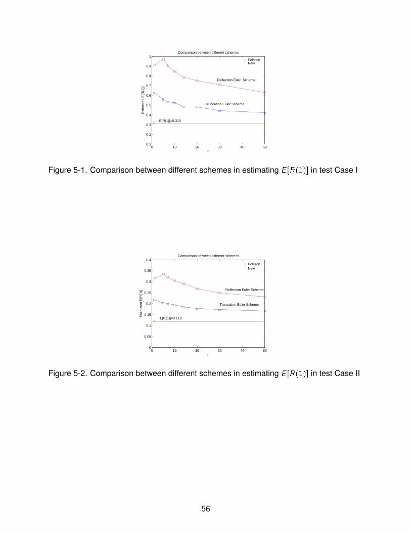
0 10 20 30 40 500.1

0.2

0.3

0.4

0.5

0.6

0.7

0.8

0.9

1PoissonNew

n

Est

imat

ed E

[R(1

)]

Comparison between different schemes

E[R(1)]=0.310

Truncation Euler Scheme

Reflection Euler Scheme

Figure 5-1. Comparison between different schemes in estimating E [R(1)] in test Case I

0 10 20 30 40 500

0.05

0.1

0.15

0.2

0.25

0.3

0.35

0.4PoissonNew

n

Est

imat

ed E

[R(1

)]


E[R(1)]=0.118



Figure 5-2. Comparison between different schemes in estimating E [R(1)] in test Case II

56

0 10 20 30 40 500

0.02

0.04

0.06

0.08

0.1

0.12

0.14

0.16

0.18

0.2PoissonNew

n

Est

imat

ed E

[R(1

)]


E[R(1)]=0.067



Figure 5-3. Comparison between different schemes in estimating E [R(1)] in test Case III

For the same set of parameters, we also tried to estimate the bond price E(e−∫1

0R(t)dt).

Here, since an integral is involved, we’ll approximate the integral by a summation, which

requires us to simulate the process on a lot of time points. Since there is no analytical

result for the expectation, we estimate it using the exact new method with 106 sample

paths and 103 time points to estimate the integral. And the estimated bond prices are

0.821, 0.913, 0.948, respectively in those three cases. With m = 10000 sample paths

and n = 10, 14, 20, 30, 50, 100 time points, we compared the performance of the Euler

schemes, the Poisson method and the exact method:

57

Table 5-5. Estimated bond price in test Case I. Numbers in parentheses are samplestandard deviations.� Euler1 Euler2 Poisson New1/10 0.749(0.003) 0.608(0.002) 0.817(0.002) 0.833(0.003)1/14 0.749(0.003) 0.632(0.002) 0.821(0.002) 0.829(0.003)1/20 0.767(0.003) 0.657(0.002) 0.819(0.002) 0.823(0.003)1/30 0.771(0.003) 0.682(0.002) 0.820(0.002) 0.826(0.003)1/50 0.776(0.003) 0.701(0.002) 0.825(0.002) 0.823(0.003)1/100 0.780(0.003) 0.722(0.002) 0.819(0.003) 0.821(0.003)

Table 5-6. Estimated bond price in test Case II. Numbers in parentheses are samplestandard deviations.� Euler1 Euler2 Poisson New1/10 0.876(0.002) 0.820(0.001) 0.913(0.001) 0.915(0.001)1/14 0.879(0.002) 0.827(0.001) 0.912(0.001) 0.913(0.001)1/20 0.884(0.002) 0.840(0.001) 0.911(0.001) 0.914(0.001)1/30 0.886(0.002) 0.853(0.001) 0.913(0.001) 0.913(0.001)1/50 0.891(0.002) 0.862(0.001) 0.912(0.001) 0.913(0.001)1/100 0.893(0.001) 0.871(0.001) 0.912(0.001) 0.913(0.001)

Table 5-7. Estimated bond price in test Case III. Numbers in parentheses are samplestandard deviations.� Euler1 Euler2 Poisson New1/10 0.921(0.001) 0.883(0.001) 0.949(0.001) 0.949(0.001)1/14 0.925(0.001) 0.888(0.001) 0.947(0.001) 0.948(0.001)1/20 0.928(0.001) 0.896(0.001) 0.948(0.001) 0.947(0.001)1/30 0.930(0.001) 0.905(0.001) 0.948(0.001) 0.948(0.001)1/50 0.933(0.001) 0.909(0.001) 0.949(0.001) 0.948(0.001)1/100 0.936(0.001) 0.919(0.001) 0.948(0.001) 0.948(0.001)

58

From the above tables, it’s easy to see that both Euler schemes still have bias in

pricing the bond price, whereas the Poisson method and our new exact method is much

more accurate. But in terms of speed, Poisson method is much slower than our new

exact method, even only 100 time points are used in the approximation of the integral.

Our new exact method remains constant speed, no matter how many time points we’re

interested in.

10 20 30 40 50 60 70 80 90 1000.6

0.65

0.7

0.75

0.8

0.85

0.9

0.95

1

n

Est

imat

ed b

ond

pric

e


Bond price=0.821



Poisson

New

Figure 5-4. Comparison between different schemes in estimating E(e−∫1

0R(t)dt) in test

Case I

59

10 20 30 40 50 60 70 80 90 1000.8

0.82

0.84

0.86

0.88

0.9

0.92

0.94

0.96

n

Est

imat

ed b

ond

pric

e


Bond price=0.913



Poisson

New


0R(t)dt) in test

Case II

10 20 30 40 50 60 70 80 90 1000.88

0.89

0.9

0.91

0.92

0.93

0.94

0.95

0.96

0.97

0.98

n

Est

imat

ed b

ond

pric

e


Bond price=0.948



Poisson

New


0R(t)dt) in test

Case III

60

5.2 Simulation Results For Heston Model

The Heston model assumes that St , the stock price and the variance processes

evolve according to the following two SDEs under the risk-neutral measure:

dSt = rStdt +√VtSt [ρdW

(1)t +

√1− ρ2dW (2)

t ],

dVt = κ(θ − Vt)dt + σ√VtdW

(1)t .

The first equation gives the dynamics of the stock price: St denotes the stock price

at time t, r is the risk neutral drift,√Vt is the volatility. The second equation gives

the evolution of the variance which follows the square-root diffusion process: θ is the

long-term level that variance gradually converges to. κ represents the speed of mean

reversion, and σ is a parameter which determines the volatility of the variance process.

W(1)t and W

(2)t are two independent Brownian motion processes, and ρ represents the

instantaneous correlation between the return process and the volatility process.

To test our new exact method, we turn to the pricing of European options in the

Heston model. This constitutes a standard test case, as prices can be computed with

great precision either from the analytical result in chapter 4, or from the FFT method in

Carr and Madan (1998) [14]. We consider a call option C maturing at time T with strike

K ; let the exact option price at time 0 be C(0). We use our exact method to simulate

V (T ), and use the approach in Anderson [4] to approximate X (T ) with X (T ). Then we

can get the approximation C(0) to the option price by computing the expectation

C(0) = E((X (T )− K)+).

In order to estimate C(0), we use Monte Carlo methods. Specifically, we draw N

independent samples of X (1)(T ), X (2)(T ), ..., X (N)(T ) using an equidistant time-grid with

61

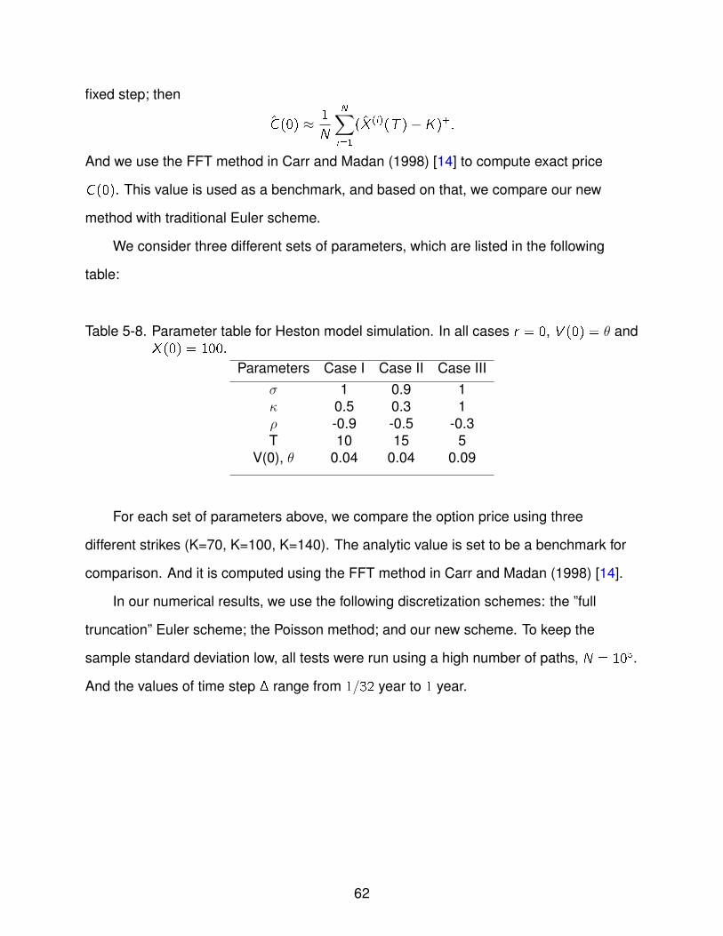
fixed step; then

C(0) ≈ 1

N

N∑i=1

(X (i)(T )− K)+.

And we use the FFT method in Carr and Madan (1998) [14] to compute exact price

C(0). This value is used as a benchmark, and based on that, we compare our new

method with traditional Euler scheme.

We consider three different sets of parameters, which are listed in the following

table:

Table 5-8. Parameter table for Heston model simulation. In all cases r = 0, V (0) = θ andX (0) = 100.

Parameters Case I Case II Case IIIσ 1 0.9 1κ 0.5 0.3 1ρ -0.9 -0.5 -0.3T 10 15 5

V(0), θ 0.04 0.04 0.09

For each set of parameters above, we compare the option price using three

different strikes (K=70, K=100, K=140). The analytic value is set to be a benchmark for

comparison. And it is computed using the FFT method in Carr and Madan (1998) [14].

In our numerical results, we use the following discretization schemes: the ”full

truncation” Euler scheme; the Poisson method; and our new scheme. To keep the

sample standard deviation low, all tests were run using a high number of paths, N = 105.

And the values of time step � range from 1/32 year to 1 year.

62

Table 5-9. Estimated European call option price in test Case I. Numbers in parenthesesare sample standard deviations.� Euler Poisson New Analytic

K=701 39.722(0.118) 36.136(0.071) 36.126(0.071) 35.8561/2 38.262(0.095) 35.937(0.071) 36.037(0.071)1/4 37.039(0.082) 35.905(0.071) 35.890(0.071)1/8 36.230(0.077) 35.997(0.071) 35.860(0.071)1/16 36.159(0.074) 35.852(0.071) 35.809(0.071)1/32 35.980(0.073) 35.899(0.071) 35.727(0.071)

K=1001 19.313(0.092) 13.308(0.042) 13.340(0.042) 13.0071/2 16.738(0.066) 13.158(0.042) 13.160(0.042)1/4 15.145(0.054) 13.120(0.042) 13.186(0.042)1/8 14.208(0.048) 13.106(0.042) 13.065(0.042)1/16 13.618(0.045) 13.075(0.042) 13.138(0.042)1/32 13.302(0.043) 13.036(0.042) 12.990(0.042)

K=1401 4.514(0.060) 0.273(0.008) 0.270(0.008) 0.3301/2 2.245(0.033) 0.279(0.008) 0.281(0.008)1/4 1.043(0.018) 0.286(0.008) 0.301(0.008)1/8 0.565(0.011) 0.289(0.008) 0.294(0.008)1/16 0.401(0.009) 0.291(0.008) 0.292(0.008)1/32 0.343(0.009) 0.293(0.008) 0.309(0.008)

63

0 5 10 15 20 25 3032

33

34

35

36

37

38

39

40

41

42

n

Est

imat

ed o

ptio

n pr

ice


option price=35.856


Poisson

New

Figure 5-7. Comparison between different schemes in estimating European option pricein test Case I (K=70)

0 5 10 15 20 25 3012

13

14

15

16

17

18

19

20

n

Est

imat

ed o

ptio

n pr

ice


option price=13.007

Poisson

New



64

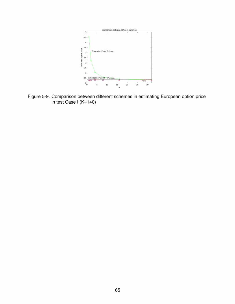
0 5 10 15 20 25 300

0.5

1

1.5

2

2.5

3

3.5

4

4.5

5

n

Est

imat

ed o

ptio

n pr

ice


option price=0.330 PoissonNew



65

Table 5-10. Estimated European call option price in test Case II. Numbers inparentheses are sample standard deviations.� Euler Poisson New Analytic

K=701 41.369(0.219) 37.012(0.141) 37.058(0.140) 36.6021/2 39.954(0.194) 37.047(0.140) 36.941(0.149)1/4 38.328(0.167) 36.981(0.139) 37.090(0.142)1/8 37.649(0.155) 36.908(0.142) 36.994(0.145)1/16 37.570(0.177) 37.127(0.139) 36.906(0.139)1/32 37.469(0.147) 36.836(0.138) 37.133(0.138)

K=1001 23.931(0.263) 16.768(0.132) 16.543(0.130) 16.2031/2 20.991(0.295) 16.637(0.148) 16.498(0.122)1/4 18.578(0.145) 16.578(0.127) 16.619(0.134)1/8 17.641(0.149) 16.620(0.134) 16.770(0.169)1/16 17.264(0.135) 16.443(0.165) 16.680(0.168)1/32 16.785(0.123) 16.386(0.122) 16.414(0.124)

K=1401 11.727(0.265) 5.146(0.112) 5.118(0.100) 4.8751/2 8.207(0.149) 5.203(0.143) 5.174(0.142)1/4 6.627(0.122) 5.184(0.133) 5.103(0.098)1/8 5.832(0.108) 5.174(0.145) 5.246(0.132)1/16 5.599(0.130) 5.101(0.102) 5.175(0.113)1/32 5.288(0.120) 5.011(0.110) 5.142(0.113)

66

0 5 10 15 20 25 3034

35

36

37

38

39

40

41

42

43

n

Est

imat

ed o

ptio

n pr

ice


option price=36.602Poisson

New


Figure 5-10. Comparison between different schemes in estimating European optionprice in test Case II (K=70)

0 5 10 15 20 25 30

14

16

18

20

22

24

26

n

Est

imat

ed o

ptio

n pr

ice


option price=16.203Poisson

New



67

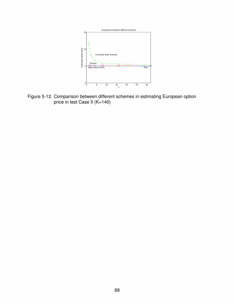
0 5 10 15 20 25 300

5

10

15

n

Est

imat

ed o

ptio

n pr

ice


option price=4.875

Poisson

New



68

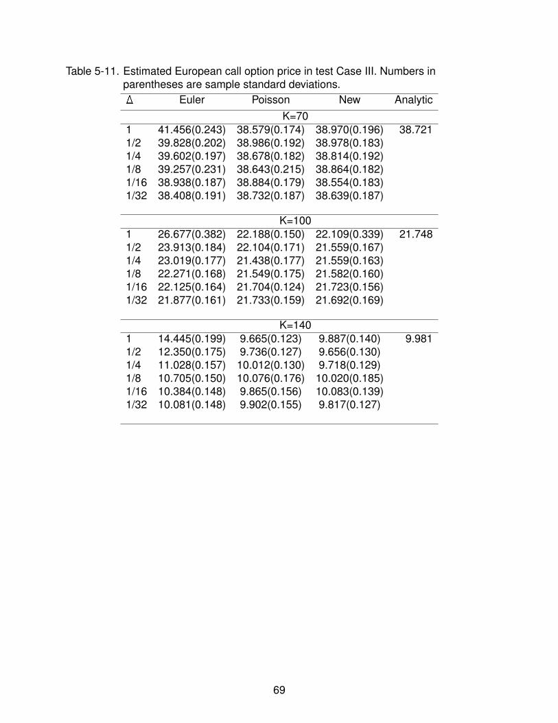
Table 5-11. Estimated European call option price in test Case III. Numbers inparentheses are sample standard deviations.� Euler Poisson New Analytic

K=701 41.456(0.243) 38.579(0.174) 38.970(0.196) 38.7211/2 39.828(0.202) 38.986(0.192) 38.978(0.183)1/4 39.602(0.197) 38.678(0.182) 38.814(0.192)1/8 39.257(0.231) 38.643(0.215) 38.864(0.182)1/16 38.938(0.187) 38.884(0.179) 38.554(0.183)1/32 38.408(0.191) 38.732(0.187) 38.639(0.187)

K=1001 26.677(0.382) 22.188(0.150) 22.109(0.339) 21.7481/2 23.913(0.184) 22.104(0.171) 21.559(0.167)1/4 23.019(0.177) 21.438(0.177) 21.559(0.163)1/8 22.271(0.168) 21.549(0.175) 21.582(0.160)1/16 22.125(0.164) 21.704(0.124) 21.723(0.156)1/32 21.877(0.161) 21.733(0.159) 21.692(0.169)

K=1401 14.445(0.199) 9.665(0.123) 9.887(0.140) 9.9811/2 12.350(0.175) 9.736(0.127) 9.656(0.130)1/4 11.028(0.157) 10.012(0.130) 9.718(0.129)1/8 10.705(0.150) 10.076(0.176) 10.020(0.185)1/16 10.384(0.148) 9.865(0.156) 10.083(0.139)1/32 10.081(0.148) 9.902(0.155) 9.817(0.127)

69

0 5 10 15 20 25 3035

36

37

38

39

40

41

42

43

44

45

n

Est

imat

ed o

ptio

n pr

ice


option price=38.721

Poisson

New


Figure 5-13. Comparison between different schemes in estimating European optionprice in test Case III (K=70)

0 5 10 15 20 25 3018

20

22

24

26

28

30

n

Est

imat

ed o

ptio

n pr

ice


option price=21.748

Poisson

New



70

0 5 10 15 20 25 306

8

10

12

14

16

18

n

Est

imat

ed o

ptio

n pr

ice


option price=9.981

Poisson New



From the above tables and graphs, we could see that the new method is more

efficient and accurate than the ”full truncation” Euler Scheme, which has a large bias in

all three cases. And as expected, Poisson method is pretty accurate but takes a much

longer time to yield the result than our new method. And as the time-step gets finer, it

will become even much slower.

Finally, we look at price of discrete Asian options under Heston’s model. Using

the parameters in case three, we use Monte Carlo method to estimate the price of a

discrete Asian call option on time interval [0, 5]. Unfortunately there is no analytical

formula for discrete Asian call option under Heston’s model. We therefore approximate

the price using our Monte Carlo simulation with m = 106 and n = 1000, and use it

as a benchmark. Once again the strike prices are K = 70, 100, 140. We would use

m = 10000 and n = 12, 30, 52, 100, 252 time points in the simulation. In this case,

Poisson method would be drastically too slow to use in simulation. Our new algorithm

turns out to be both accurate and efficient.

71

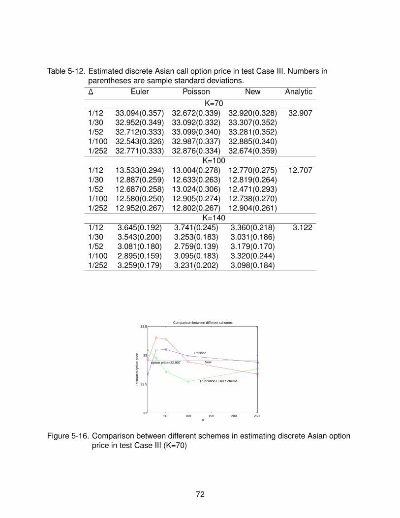
Table 5-12. Estimated discrete Asian call option price in test Case III. Numbers inparentheses are sample standard deviations.� Euler Poisson New Analytic

K=701/12 33.094(0.357) 32.672(0.339) 32.920(0.328) 32.9071/30 32.952(0.349) 33.092(0.332) 33.307(0.352)1/52 32.712(0.333) 33.099(0.340) 33.281(0.352)1/100 32.543(0.326) 32.987(0.337) 32.885(0.340)1/252 32.771(0.333) 32.876(0.334) 32.674(0.359)

K=1001/12 13.533(0.294) 13.004(0.278) 12.770(0.275) 12.7071/30 12.887(0.259) 12.633(0.263) 12.819(0.264)1/52 12.687(0.258) 13.024(0.306) 12.471(0.293)1/100 12.580(0.250) 12.905(0.274) 12.738(0.270)1/252 12.952(0.267) 12.802(0.267) 12.904(0.261)

K=1401/12 3.645(0.192) 3.741(0.245) 3.360(0.218) 3.1221/30 3.543(0.200) 3.253(0.183) 3.031(0.186)1/52 3.081(0.180) 2.759(0.139) 3.179(0.170)1/100 2.895(0.159) 3.095(0.183) 3.320(0.244)1/252 3.259(0.179) 3.231(0.202) 3.098(0.184)

50 100 150 200 25032

32.5

33

33.5

n

Est

imat

ed o

ptio

n pr

ice


option price=32.907

Poisson

New


Figure 5-16. Comparison between different schemes in estimating discrete Asian optionprice in test Case III (K=70)

72

50 100 150 200 25011

11.5

12

12.5

13

13.5

14

14.5

15

n

Est

imat

ed o

ptio

n pr

ice


option price=12.707

Poisson

NewTruncation Euler Scheme


50 100 150 200 2502.5

3

3.5

4

4.5

n

Est

imat

ed o

ptio

n pr

ice


option price=3.122

Poisson

New



73

CHAPTER 6CONCLUSION

In this paper, a fast and efficient way of simulating CIR process is introduced. We

proved a theorem that could be used to generate a non-central Chi-square random

variable. And the way we generate it avoids the problem with the traditional method that

involves Poisson random variable generation. Our new method is exact compared with

Euler schemes, and fast compared with Poisson method. Especially in the case when

d << 1 and we need to simulate a CIR process along many time points, traditional

Poisson method is very slow since the non-centrality parameter is big. On the other

hand, our new method for generating a CIR process is independent of the number of

time points needed in the simulation, thus much quicker than the Poisson method. We

proposed several numerical tests to test our algorithm and the results have shown that

our method is very efficient and suitable to be used in this particular case.

74

REFERENCES

[1] Alfonsi, A. “On the discretization schemes for the CIR processes.” Monte carlomethods and applications 11 (2005).4: 355–467.

[2] ———. “A second-order discretization scheme for the CIR process: application tothe Heston model.” preprint (2008).

[3] ———. “High order discretization schemes for the CIR process: Application toaffine term structure and Heston Models.” Math. Comput. 79 (2010).269: 209–237.

[4] Anderson, L. “Efficient simulation of the Heston stochastic volatility model.” Journalof computational finance 11 (2007): 1–42.

[5] Bandorff-Nielsen, O. “Process of Normal Inverse Gaussian Type.” Finance andStochastics 2 (1998): 41–68.

[6] Berkaoui, A., Bossy, M., and Diop, A. “Euler scheme for SDEs with non-Lipschitzdiffusion coefficient: strong convergence.” ESAIM Probability and Statistics 12(2008).1: 1–11.

[7] Black, F. and Karasinski, P. “Bond and Option pricing when Short rates areLognormal.” Financial Analysts Journal (1991): 52–59.

[8] Black, Fischer and Karasinski, Piotr. “Bond and option pricing when short rates arelognormal.” Financial Analysts Journal July/August (1991): 52–59.

[9] Black, Fischer and Scholes, Myron. “The Pricing of Options and CorporateLiabilities.” Journal of Political Economy 81 (1973).3: 637–654.

[10] Brennan, Michael J. and Schwartz, Eduardo S. “An equilibrium model of bondpricing and a test of market efficiency.” Journal of Financial and QuantitativeAnalysis 17 (1982): 75–100.

[11] Brigo, D. and Alfonsi, A. “Credit default swap calibration and derivatives pricing withthe SSRD stochastic intensity model.” Finance and Stochastics 9 (2005).1: 29–42.

[12] Broadie, M. and Kaya, O. “Exact simulation of stochastic volatility and other affinejump diffusion processes.” Operational Research 54 (2006): 217C231.

[13] Carr, P., Geman, H., Madan, D.B., and Yor, M. “The fine structure of asset returns:an empirical investigation.” Journal of Business 75(2) (2002): 305–332.

[14] Carr, P. and Madan, D. “Option Valuation using the Fast Fourier Transform.” Journalof Computational Finance 2 (1998): 61–73.

[15] Carr, P. and Wu, L. “The finite moment log stable process and option pricing.”Jounal of Finance 58(2) (2003): 753–777.

75

[16] Christie, A.A. “The stochastic behavior of common stodck variances.” Journal ofFinancial Economics 10 (1982): 407–432.

[17] Cox, J.C, Ingersoll, J.E., and Ross, S.A. “A theory of the term structure of interestrates.” Econometrica 53 (1985): 385–407.

[18] David, Bates. “The crash of 87: Was it expected? The evidence from optionsmarkets.” Journal of Finance 46 (1991): 1009–1044.

[19] Deelstra, G. and Delbaen, F. “Convergence of discretized stochastic (Interest rate)processes with stochastic drift term.” Appl. stochastic models data anal. 14 (1998):77–84.

[20] Dilip, Madan and Chang, Eric. “The Variance Gamma Model and Option Pricing.”European Finance Review 2 (1998): 79–105.

[21] Dothan, Uri L. “On the term structure of interest rates.” Journal of FinancialEconomics 6 (1978): 59–69.

[22] Eberlein, E., Keller, U., and Prause, K. “New insights into smile, mispricing, andvalue at risk: the hyperbolic model.” Journal of Business 71(3) (1998): 371–405.

[23] Elias, Stein and Stein, Jeremy. “Stock price distributions with stochastic volatility.”Review of Financial Studies 4 (1991): 727–752.

[24] Fama, Eugene F. “The Behavior of Stock Market Prices.” Journal of Business 38(1965): 34–105.

[25] Feller, W. “Two Singular Diffusion Problems.” Annals of Mathematics 54 (1951):173–182.

[26] Glasserman, P. Monte Carlo methods in financial engineering. New York:Springer-Verlag, 2003.

[27] Heston, S. “A closed-form solution of options with stochastic volatility withapplications to bond and currency options.” The review of financial studies 6(1993).2: 327–343.

[28] Hull, John and White, Alan. “The pricing of options with stochastic volatilities.”Journal of Finance 42 (1987): 281–300.

[29] ———. “Pricing interest-rate derivative securities.” Review of Financial Studies 3(1990): 573–592.

[30] Istvan, G. and Miklos, R. “A note on Euler approximations for SDEs with Hodercontinuous diffusion coefficients.” stochastic processes and their applications 121(2011).10: 2189–2200.

[31] John, Cox and Ross, Stephen. “The valuation of options for alternative stochasticprocesses.” Journal of Financial Economics 3 (1976): 145–166.

76

[32] Kahl, C. and Jackel, P. “Fast strong approximation Monte-Carlo schemes forstochastic volatility models.” J. Quantit. Finance 6 (2006): 513–536.

[33] Kaushik, Amin and Jarrow, Robert. “Pricing options on risky assets in a stochasticinterest rate economy.” Mathematical Finance 2 (1992): 217–237.

[34] Kloeden, P.E. and Platen, E. Numerical solution of stochastic differential equations.Berlin: Springer-Verlag, 1992.

[35] Mandelbrot, B.B. “The variation of certain speculative prices.” Journal of Business36 (1963): 394–419.

[36] Melino, Angelo and Turnbull, Stuart. “Pricing foreign currency options withstochastic.” Journal of Econometrics 45 (1990): 239–265.

[37] Merton, R. C. “Option pricing when underlying stock returns are discontinuous.”Journal of Financial Economy 3 (1976): 125–144.

[38] Merton, Robert C. “Theory of rational option pricing.” Bell Journal of Economicsand Management Science 4 (1973): 141–183.

[39] Samuelson, P.A. “Proof that Properly Anticipated Prices Fluctuate Randomly.”Industrial Management Review 6 (1965): 41–49.

[40] Scott, E. and Tucker, A. L. “Predicting currency return volatility.” Journal of Bankingand Finance 13 (1989).6: 839–851.

[41] Scott, Louis. “Option pricing when the variance changes randomly: Theory,estimators, and applications.” Journal of Financial and Quantitative Analysis 22(1987): 419–438.

[42] Vasicek, O. “An equilibrium characterization of the term structure.” Journal ofFinancial Economics 5 (1977): 177–188.

[43] Wiggins, James. “Option values under stochastic volatilities.” Journal of FinancialEconomics 19 (1987): 351–372.

77

BIOGRAPHICAL SKETCH

Anqi Shao was born in Urumqi, China in 1982. He moved to Yantai with his family in

1994 and attended No. 1 high school there. He went to the department of mathematics

in 1999, and got his bachelor’s degree from Shandong University in 2003. He then went

to graduate school at Lehigh University in 2004, and transferred to University of Florida

in 2005. He received Master of Science in mathematics in 2008 and Master of Statistics

in 2009. He completed his doctorate of philosophy in the area of mathematical finance in

the summer of 2012.

78

c 2012 Anqi Shao - University of Floridaufdcimages.uflib.ufl.edu/UF/E0/04/39/21/00001/SHAO__.pdf ·...

Documents

Transcript of c 2012 Anqi Shao - University of Floridaufdcimages.uflib.ufl.edu/UF/E0/04/39/21/00001/SHAO__.pdf ·...