TECHNICAL'REPORT ECOM C-0423-1

(Q GASEOUS PLUME DIFFUSION

(0: CHARACTERISTICS WITHIN MODEL

PEG CANOPIES

0 TASK IIB RESEARCH TECHNICAL REPORT

*e DESERET TEST CENTER

0* BYS

* R. N. MERONEYD. KESIC .'

* and

* T. YAMADA FE

0SEPTEMBER 1968

~DISTRIBUTION OF THIS DOCUMENT IS UNLIMITED

UNITED STATES ARMY ELECTRONICS COMMAND FORT MONM .OUTH, N. J.

CON-.-RACT DAAB07=68=C=0423FLUID DYANAMICS AND DIFFUSION LABORATORYFLUID MECHXICS PROGkAMCOLLEGE OF ENGINEERINGCOLORADO STATE UNIVERSITY ... -

FORT COLLINS, COLORADO 80521

0I

BL7 A.iiow

I .. ,**DISCLAIMER

~-.~jT EiTATION OF TRADE NAMES AND NAMES OF MANUFACTURERS IN THIlS REPORT

IS NOT TO BE CONSTRUED AS OFFICIAL GOVERNMENT INDORSEMENT OR APPROVAL

OF COi.iERCIAL PRODUCT'S OR SERVICES REFERENCED) HEREIN.

4

Technical Report ECOM C-0423-1 September 1968

Wind Tunnel Studies and Simulations

of Turbulent Shear Flows Related to

Atmospheric Science and Associated Technologies

TECHNICAL REPORT

GASEOUS PLUME DIFFUSION

CHARACTERISTICS WITHIN MODEL

PEG CANOPIES

TASK IIB RESEARCH TECHNICAL REPORT

DESERET TEST CENTER

PREPARED BY

R. N. MERONEY

D. KESIC

and

T. YAMADA

Fluid Dynamics and Diffusion Laboratory

Fluid Mechanics Program

College of Engineering

Colorado State University

Fort Collins, Colorado

80521

for

ATMOSPHERIC SCIENCES LABORATORY

U. S. Army Electronics Command

Fort Monmouth, N. J.

CER68-69RNM-DK-TY-3

ABSTRACT

A point source of an air-helium mixture was released

continuously at various positions within a simulated canopy composed

of 9 cm high pegs, 0. 48 cm diameter, spaced in several arrays

(2.54 x 2.54, 3.55 x 3.55, and 5.08 x 5.08 cm). Variations of the

vertical location of the source revealed the strongly nonisotropic

character of diffusion within a canopy with respect to the relative

diffusion rates in the lateral and vertical direct; ns. When the source

was placed at various downstream distances from the edge of the can-

opy, it displayed a tendency to exhale the plume near the front of the

model canopy and to inhale the plume at distances further downstream.

Calculations of the turbulent diffusion coefficient, K, within and above

the canopy from the experimental data, reveal both a constant region

and a region of linear increase with height increase as suggested by

previous authors,

ii

TABLE OF CONTENTS

Page

LIST OF FIGURES.......................... iv

INTrRODUJCIO~N.. .. .. .. .... . .. .. .. .. .. .. 1I

MODELING OF A VEGETATIVE CANOPY............... 4

EXPERIMENTAL EQUIPMENT AND PROCEDURE ....... 6

EXPERIMENTAL RESULTS..........................9

CONCLUSIONS ............ . ............. 18

BIBLIO1GR1APHY............................ 20

FIGURES . ......... . 0 ....... 23

LIST OF FIGURES

Figure Page

1 Wind tunnel and artificial canopy configuration ......... 24

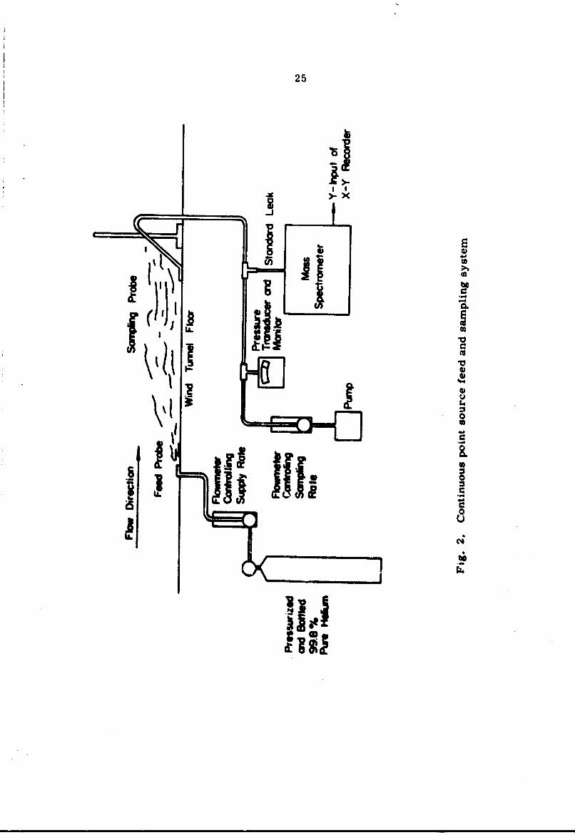
2 Continuous point source feed and sampling system..... .25

3 Velocity profiles within model canopy ................ 26

4 Velocity profiles above model canopy .............. 27

5 Longitudinal turbulent intensity for model canopy .. .. 28

6 Vertical turbulent intensity for model canopy .......... 29

7 Shear profile for model canopy. . . . . . ......... 30

8 Streamline flow in and above a model canopy. . . . . . 31

9 Vertical dispersion of a continuous point sourcein a model peg canopy (2. 54 x 2. 54 cm) x =0,z - 1cm . . . . . . . . . . . . . . . . . . .. . . . . . .. . 32

s

10 Vertical dispersion of a continuous point source ina model peg canopy (2. 54 x 2. 54 cm). x5 = 0z =-0. 5 h . . . . . . . . . . . . . . . . .. . . . . . . .. . 33

s

11 Vertical dispersio A a continuous point sourcein a model peg canopy (2. 54 x 2. 54 cm). x - 0,z = h . . . . . . . . . . . . . . . . . . . . . . . . . . . .34

12 Vertical dispersion of a continuous point sourcein a model peg canopy (2. 54 x 2. 54 cm). x 6 m,zs lcm . . . . . . . . . . . . . . . . . . . . . . . . . . . 35

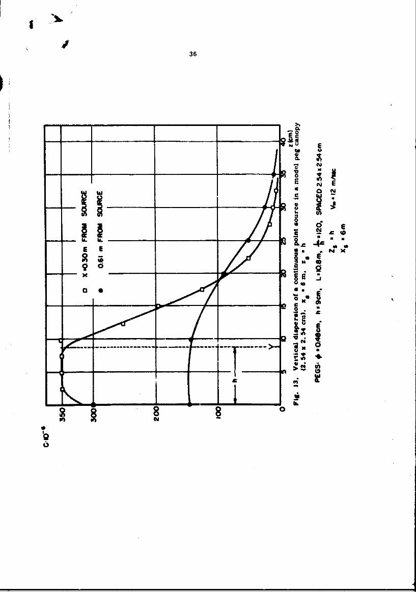
13 Vertical dispersion of a continuous point sourcein a model peg canopy (2.54 x 2.54 cm). x 6 m,

S

14 Vertical dispersion of a continuous point source ina model peg canopy (2. 54 x 2. 54 cm). x 6 1,

iv

I

LIST OF FIGURES - Continued

Figure Page

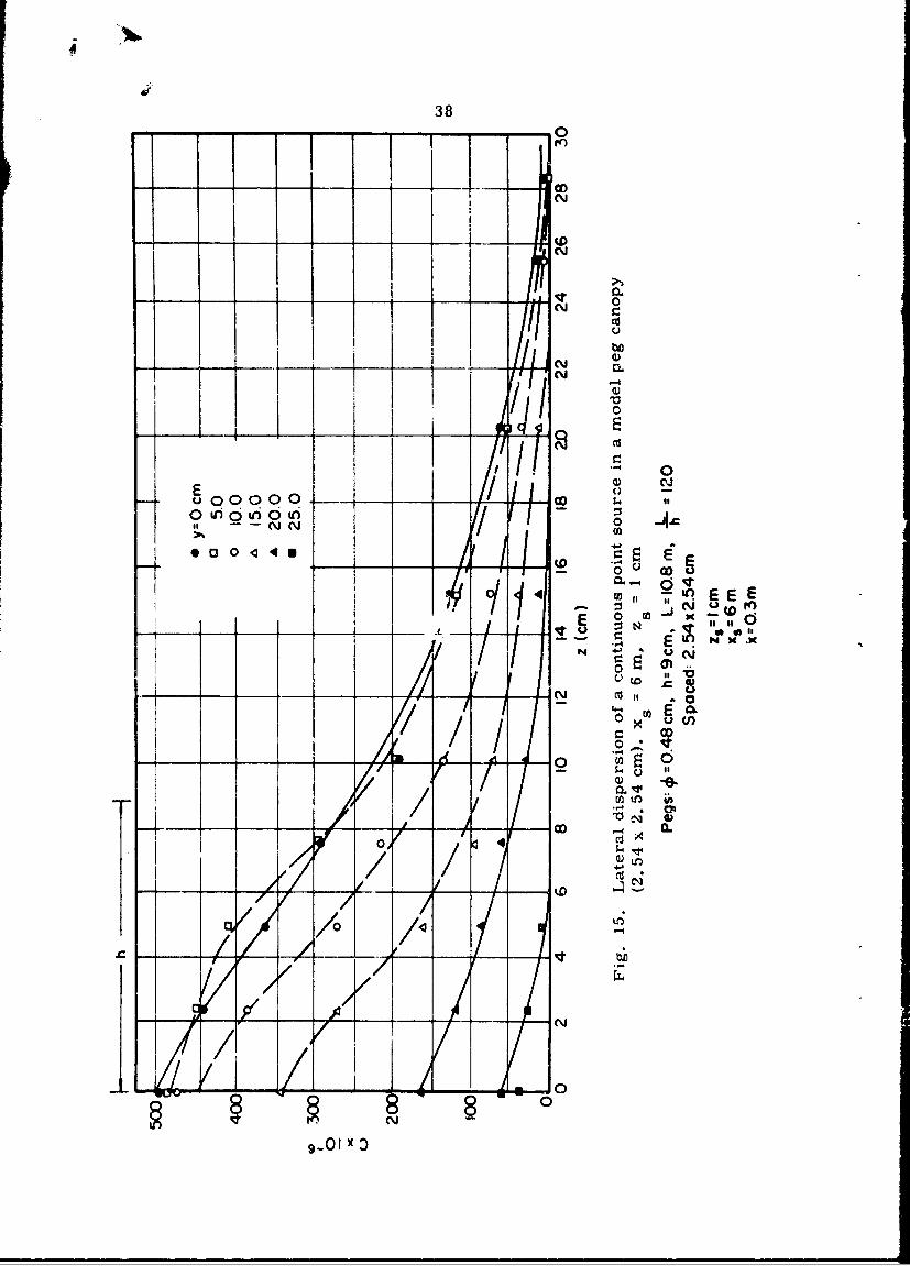
15 Lateral dispersion of a continuous point sourcein a model peg canopy (2. 54 x 2. 54 cm). x = 6 m,z 1 cm. ........................... 38s

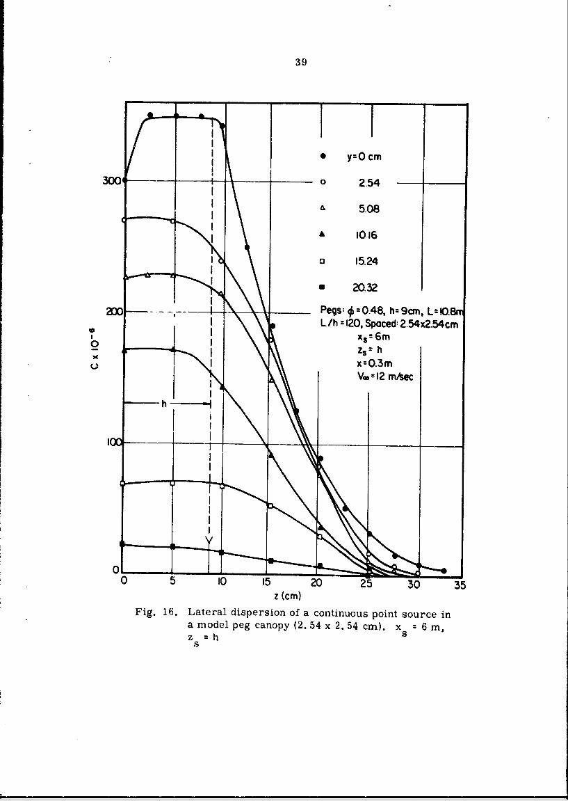
16 Lateral dispersion of a continuous point sourcein a model peg canopy (2. 54 x 2. 54 cm). x = 6 m,5z =h .............................. . ........ . 39s

17 Lateral dispersion of a continuous point sourcein a model peg canopy (2. 54 x 2.54 cm). x z 6 m.z = 1 cm ............ ................. ...... . 40s

18 Lateral dispersion of a continuous point sourcein a model peg canopy (2. 54 x 2. 54 cm). x = 6 m,5z =h . . . . . . . . . . . . . . . . . . . . . . . . . .. 41

s

19 Vertical dispersion of a continuous point sourcein a model peg canopy (2. 54 x 2.54 cm diagonal).x = 0. z = 1 cm . . . . . . . . . . . . . . . . . . . . . . 42

5 5

20 Vertical dispersion of a continuous point sourcein a model peg canopy (2. 54 x 2.54 diagonal).x s =00 z s= 0.5 h .. .. .. .. .. .. .. .. .. . .. 43

21 Vertical dispersion of a continuous point sourcein a model peg canopy (2. 54 x 2. 54 diagonal).x =0, z =h . . . . . . . . . . . . . . . . . . . .. . . 44

22 Vertical dispersion of a continuous point sourcein a model peg canopy (2. 54 x 2.54 diagonal).x -6 m. z z--lcm . . . . . ......... 0 . ... 45

23 Vertical dispersion of a continuous point sourcein a model peg canopy (2. 54 x 2. 54 diagonal).x 6 m, z 0.5h . ................... 46

24 Vertical dispersion of a continuous point sourcein a model peg canopy (2. 54 x 2. 54 diagonal).x -6 m, z -h . . . . . . . . . . . . . . . . . . . . . . 47

25 Vertical dispersion of a continuous point sourcein a model peg canopy (2. 54 x 2. 54 diagonal).x s 6m, z - l. Sh . ............... . . . . . . 48

s 5

V

LIST OF FIGURES - Continued

Figure Page

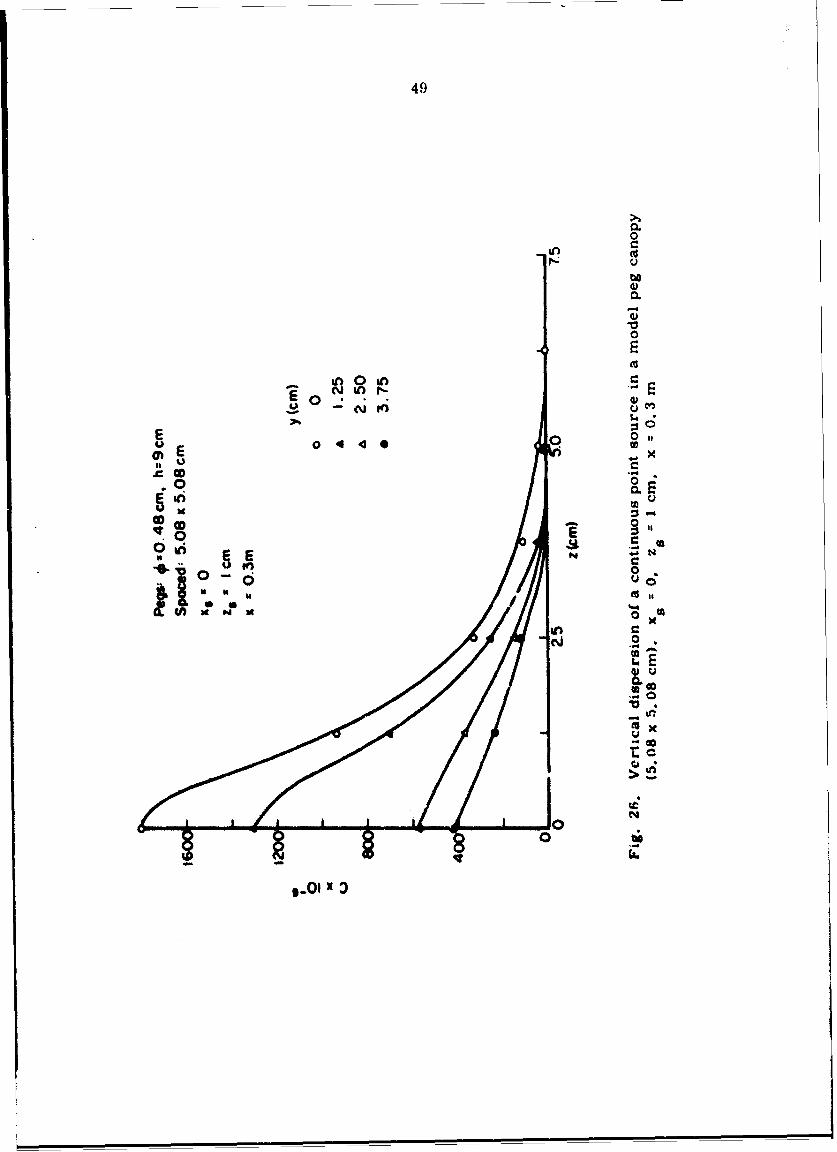
26 Vertical dispersion of a continuous point sourcein a model peg canopy (5. 08 x 5. 08 cm). x = 0,Sz = 1 cm, x = 0.3 m ...... ..................... 49

s

27 Vertical dispersion of a continuous point sourcein a model peg canopy (5.08 x 5.08 cm). x = 0,s

z s1=cm, x = 0.6m ..... ................... .50s

28 Traces of maximum concentration from a pointsource (2.54x 2.54 cm). x = 0, z = 0.5h ........ 51

29 Traces of maximum concentration from a pointsource (2.54x2.54cm). x =0, z =h . . . . . . . . . .52

30 Diliusion in the canopy-isoconcentration lines(2.54x 2.54 diagonal). x = 0, z = 1 cm. . . . . . . . . .53s 5

31 Diffusion in the canopy-isoconcentration lines(2.54x 2.54 diagonal). x -=0, z = 0.5h . . . . . . . . .54

32 Diffusion in the canopy-isoconcentration lines(2. 54 x 2. 54 diagonal). xs %. 0, z -- h . . . .. . ..... 55

33 Duflusion in the canopy-isoconcentration lines(2.54x 2.54 diagonal). x = 6, z 8= crn . .. ... . * * .56

34 Diffusion in the canopy-isoconcentration lines(2.54x 2.54 diagonal). x 8 x 6. z a 0.5 h * . s ... . . .57s s

35 Diffusion in the canopy-isoconcentration lines(2.54x 2. 54 diagonal). x 8 6, z w h ••....... .58s s

36 Diffusion in the canopy-isoconcentration lines(2,54 x 2.54 diagonal). x s a 6. 2 1.5h. . . . . . . . . .59

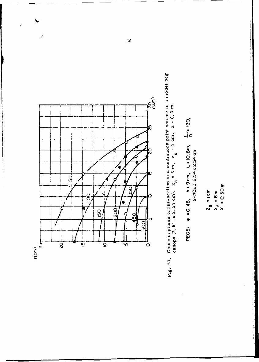
J? Gaseous plume cross-section of a continuouspoint source in a model peg canopy (2. 54 x ?. 54 cm).x a 6 m, z. 2 1 cm, x r 0.3 m . . 0 * .. . .. . . . # 60

38 Gaseous plume cross-section of a continuouspoint source in a model peg canopy (2. 54 x 2. 54 cm).x a6m, z : h. x 0. 3 m . . . . . . . . . . . . . . . . .61

S v

vi

4,

LIST OF FIGURES - Continued

Figure Page

39 Gaseous plume cross-section of a continuouspoint source in a model peg cano -" (2. 54 x 2. 54cm diagonal). x = 6m, z = 1 cm, x = 0.25m . . .. 62

5 S

40 Gaseo-:.- plume cross-section of a continuouspoint source in a model peg canopy (2. 54 x 2. 54cm diagonal). : C -, z = h, x = 0. 5m . . . . 63S 5

41 Gaseous plume cross-section of a continuouspoint source in a model peg canopy (5.08 x 5.08cm). x = 0 m, z = 1 cm, x = 0.3 m . . .... ...... 64

42 Gaseous plume cross-section of a continuouspoint source in a model peg canopy (5.08 x 5.08cm). x = 0m, z =1 cm, x= 0.6m . . . . . .. .. . 65

5 5

43 Variation of ground level concentration withdownstream distance . . . . . . . . . . . . . . . .... 66

44 Variation of characteristic plume height withdownstream distance . . . . . . . . . . . . . . . . . . . 67

45 Coefficient of turbulent diffusion . . . . . . . . . . . . . 68

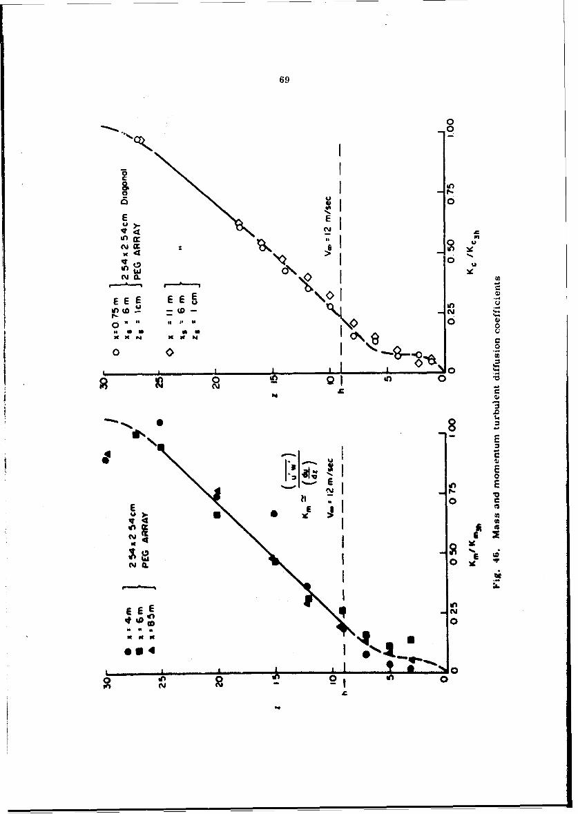
46 Mass and momentum turbulent diffusion coefficients . . 69

47 Dimensionless eddy diffusion coefficient. . . . . . . . . 70

vii

GASEOUS PT,UME DIFFUSIONCHARACTERISTICS WITHIN MODEL

PEG CANOPIES

by

R. N. Meroney*, , D. Kesic*"and T. Yamada**

INTRODUCTION

Agricultural meteorologists, atmospheric scientists, and

many hydrologists are interested in the evaporation and exchange

processes which occur in vegetative canopies. Such information

permits calculation of the efficiency of water, energy, and C0 2

transport in plant metabolism and the penetration of foreign .:.oditives

into or their escape out of the bulk of a canopy. As early as 1937

experimenters have made measurements of velocity, temperature,

evaporation rateb, atid energy balance within and above such con-

figurations 1.2,3.4 These measurements have provided a rough

picture of a highly complex and turbulent now field within the vege-

tation. Today, there exists a definite need for more elaborate and

extensive measurements for different types of simple geometry crops.

*Assistant Professor of Civil Engineering, Coloradv State University**Graduate Research Assistants. Department of Civil EngineerinG.

Colorado State University

2

Past measurements of diffusion from point or line sources in

such configurations seem to have been limited to measurements of

an instantaneous line source by Bendix over a tropical rain forest,

of point and line source distributions over a deciduous forest by

15Litton Systems, of instanteous point sources in a jungle-like

i6deciduous forest by Melpar, and of rates of particulate dispersion

in a forest canopy at Brookhaven. 6 These measurements are extensive

and well documented; however, they must be normalized to some

simplified geometry in order to det'eriine the universal

characteristics and governing parameters of vegetative penetration

by a diffusing plume.

Since field measurements ire :oot easy to obtain because of the

cost of providing a perfect measuring station and the difficulty of

obtaining cooperative weather, a laboratory program of modeling

the flow in and above plant covers has been initiated at the Fluid

Dynamics and Diffusion Laboratory at Colorado State University.

Previous results from this program have been published by Quarishi

and Plate, Yano, Hsi and Nath, and Kawatani. 8,17,18

The purpose of thic report is to discuss some measurements of

diffusion from a continuous point source in and above a model peg

canopy. The results of this study will consist of:

1) A description of the diffusion processes in and above the

simulated canopy,

3

2) A description of the vertical dispersion of the tracer mater;als,

3) A determination of the effect of the initial fetch of the peg

canopy on tracer dispersion, and, finally,

4) A determination of the vertical distribution of the eddy

diffusion coefficients in and above the modeled canopy.

4

MODELING OF A VEGETATIVE CANOPY

The wind tunnel, long a research tool of the aerodynamicist,

has recently proven its worth in atmospheric science through the

success of an extensive sequence of programs to study modeling

feasibility for micro-meteorological research. 9,10 As a result, it

is now possible, for those conditions where Coriolis effects are

secondary, to model many important features of the atmosphere.

Suggestions concerning the applicable modeling criteria for vege-

7tative canopies have been made by Quarishi and Plate.

The intent of this program was to scale the nature of gaseous

plume penetration at different points above a model crop, to

determine the dispersion characteristics of a plume in such circum-

stances, and then to calculate and compare eddy diffusion coefficients

with prototype data. Rather than model specifically all the complex

characteristics of a live vegetative cover, it was proposed to retain

the character of the flow while avoiding its minute complexity. Hence,

short dowel pegs, approximately 0. 5 cm in diameter and 9 cm long,

were chosen as model elements and arranged in various geometrical

patterns. This rough boundary arrangement produced turbulent flow

at even small velocities; a constant drag coefficient, independent of

wind speed*; and, hence, a flow independent of Reynolds' number.

*Measurements of canopy drag force were made by a shear plate

described in Army Quarterly Report No. 11, 1 Nov 67-31 Jan 68,grant DA-AMC-28-043065-G20.

5

A logarithmic velocity profile similar to that typically found in the

vertically stratified atmospheric boundary layer was reproduced

in the wind tunnel by an upstream fetch of 20 meters of test section

floor. It has been repeatedly shown that such an upstream boundary

condition is critical for the quivalent kinematic character of a

modeled flowfield. 9, 10, 19

A careful study of the mean velocity profiles, turbulent inten-

sities and shear stress in and above the model peg canopy has been

18completed by Kawatani. These data were compared with prototype

measurements in forests and agricultural crops. The marked func-

tional agreement between the dynamic and kinematic behavior of the

peg canopies and the live vegetative canopies provided a confirmation

of the assumption of general similarity.

6

EXPERIMENTAL EQUIPMENT AND PROCEDURES

The experimental data were obtained in the low speed Army

Meteorological Wind Tunnel in the Fluid Dynamics and Diffusion11

Laboratory at Colorado State University. This tunnel was specif-

ically designed to study fluid phenomena of the atmosphere. It has

a 2 meter square by 26 meter long test section with an adjustable

ceiling to provide a zero pressure gradient over the canopy crop.

Model elements consisted of 0. 48 cm diameter by 9 cm long dowel

pegs inserted in holes in aluminum plate sections and arranged in

geometric arrays the width of the test section extending for 11 meters

downstream from the middle of the length dimension of the tunnel.

All the various arrangements studied are summarized in Fig. 1.

A single and a cross-wire constant temperature anemometer

was used to measure velocity, turbulent intensity, and shear. In

addition, pitot-static tube measurements were made at each section.

The sending elements of the anemometer circuit were platinum wire

0. 2 mil in diameter and approximately 0. 25 cm long. The bridge

circuit utilized was a CSU Solid State Anemometer and the pitot tube

output went to a Transonic Mod l A, Type 120 electronic pressure meter.

Turbulence signals were interpreted by : eans of a CSU designed sum

and difference circuit and a Bruel and Kjaer RMS meter, Model 2416.

'7

Helium gas was used as a tracer for the turbulent diffusion

experiments. The gas was released continuously at a constant rate

of 630 cc/min from a 2 mm nozzle located in or above the canopy. The

sampling probe, manufactured from small diameter hypodermic

tubing, was mounted on a traversing carriage, the horizontal and

vertical positions of which were controlled remotely from outside the

tunnel. Helium concentration was measured at ground level along a

line normal to the axis of the plume and vertically at the plume

centerline.

Samples were drawn into the probe at a constant rate and passed

over a standard leak into a mass spectrometer (Model MS9AB of the

Vacuum Electronic Corporation). Output of the mass spectrometer

was an electrical voltage proportional to concentration. The mass

spectrometer was calibrated periodically be a set of pre-mixed

gases of research grade. Fig. 2 shows the experimental

arrangment.

Since a closed-circuit wind tunnel was used, the ambient

concentration level of helium built up in the wind tunnel with time.

Eventually, most of the gas did leak out; therefore the amount of

helium in the ambient flow was never higher than 60 parts per

million. Nevertheless, an ambient concentration measurement was

taken after each profile. The relative concentration was obtained

8

by subtracting the corresponding ambient concentration from the

absolute concentrati)n. All data rresented in the figures or tables

are relative concentrations.

Due to the slow response of the mass spectrometer, a period

of one to two minutes was allocated for the stabilization of each

reading before it was recorded. Usually, the concentration signal

itself was averaged (over at least 60 seconds. This method gave

results that compared favorable with the average of signals taken

over a period as long as 250 seconds by graphical means.

9

EXPERIMENTAL RESULTS

All measurements were taken at a free stream velocity of

12 m/sec. The ceiling of the test section was adjusted for zero

pressure gradient, and the upstream velocity profile was measured

and found to be logarithmic. And, because the temperature condition

was constant, neutral stability existed.

1. Typical Velocity, Streamline, and Shear Results

Velocity and shear measurements have been compiled for pegs

positioned in 1. 27 x 1. 27 cm diagonal, 2. 54 x 2. 54 cm square, 2. 54 x

2. 54 cm diagonal and 5. 08 x 5. 08 cm square arrays. In the downwind

direction, the typical transformations of the wind profiles in the

vertical direction are shown in Figs. 3 and 4 for flow in and above

the crop respectively. Velocity profiles within the canopy agree1.2,3,4

qualitatively with prototype measurements, and approximate

the exponential profiles suggested by Inoue, Saito and Cionco, (et al).

2,12,13 The profiles above the canopy are logarithmic and follow the

displacement law u/u* - 1/k In [(y-d)/zo] utilized for rough surfaces

since the time of Rossby and Montgomery (1935).

Typical intensity and shear profiles shown in Figs. 5, 6 and 7

indicate the growth of the inner boundary layer over the rough surface.

The shear profile growth compares favorably with the measurements

of transition made by Schlichting for flow from a smooth to a rough

10

14surface. Values of intensity from 0. 5 to 0. 8 within the canopy

correspond to field measurements in crops and forests but suggest

that a linearized interpretation of the hot-wire anemometer output

is extremely doubtful. Hence, measurements of velocity, intensity

or shear may err as much as 20% at the lower velocities.

Streamline calculations over the model canopy as shown in Fig.

8 indicate the tendency for the approach flow to initially accelerate

upward away from the floor and then to subsequently re-penetrate

the canopy ceiling. This flow behavior was also evidenced in the

diffusion measurements. It was concluded that the flow field was

probably quasi-established within 60 h of the inception of the canopy.

The dynamic behavior of the flow over the peg canopies is described

in greater detail in Reference 18.

2. Diffusion Plume Results

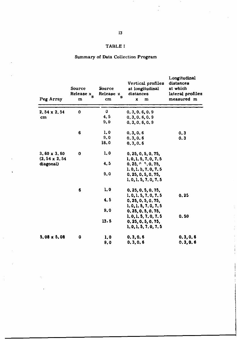
Diffusion measurements were made over pegs positioned in the

2. 54 x 2. 54 cm square, 2. 54 x 2. 54 cm diagonal (3. 60 x 3. 60 cm)

and 5. 08 x 5.08 cm square arrays (see Table I). The plume source

was located either at the canopy inception (x8 -- 0) or six meter s

downstream (x -- 6 m). It was located at various times at heights

of lcm, 4. 5 cm, 9 cm and 13.5 cm (za = 1 cm, h/2, h, 3/2 h).

Vertical and horizontal traverses along the plume were made at

varying distances downstream.

11

Source and sampling tube locations studied are summarized in

Table 1. The most extensive data are available for the 2. 54 x 2. 54

diagonal (or center filled square) matrix. Unfortunately, the program

of diffusion measurements was instituted some time after the inception

of the dynamic measurements (mean velocity, turbulence, etc.), and

therefore only a limited number of data are presented for the other

peg matrices.

Figures 9 to 18 display the loigitudinal variation of the vertical

profiles for the 2. 54 x 2. 54 cm peg matrix. Figures 15 to 27 display

the longitudinal variation of the vertical profiles for the 2. 54 x 2. 54

cm diagonal peg matrix. The lateral profiles for the 2. 54 x 2. 54.

2. 54 d x 2. 54 d and the 5. 08 x 5. 08 cm peg matrices are displayed

as isoconcentration lines on Figs. 37-38. 39-40 and 41-42. respectively.

The more extensive concentration data for the 2. 54 x 2. 54 diagonal

peg matrix have been converted into isoconcentration profiles for a

longitudinal section along the plume centerline. Figures 30 to 32

indicate the tendency of a point source to exhale out of the canopy

when the source is located at half canopy height or above and near the

inception of the vegetative cover. Farther downstream, the plume

tends to dip down into the vegetative cover when released above the

canopy, as is shown in Figures 33 to 36.

Figures 28 and 29 show how the plume maximum concentration

rises abruptly upward at the canopy inception and subsequently is

12

displaced downward slightly as the flow re-penetrates the canopy

ceiling. In the same figures, the maximum concentration line is

compared with the meandering of the streamlines passing through

the source position.

13

TABLE I

Summary of Data Collection Program

Longitudinal

Vertical profiles distancesSource Source at longitudinal at whichRelease x Release z distances lateral profiles

Peg Array m cm x m measured m

2.54x2.54 0 0 0.3,0.6,0.9cm 4.5 0.3, 0.6, 0.9

9.0 0.3,0.600.9

6 1.0 0.3,0.6 0.39.0 0.3.0.6 0.3

18.0 0.3.0.6

3.60 x 3.60 0 1.0 0.25,0.5,0.75,(2.54 x 2.54 1.0,1.5,7.0.7.5diagonal) 4.5 0.25, n - 0.75.

1.0,1. ,7.0. 7.59.0 0.25,0.5,0.75,

1.0,1. 5, 7.0, 7.5

6 1.0 0.25,0.5,0.75.1.0.1.5,7.0, 7.5 0.25

4.5 0.25,0.5,0.75,1.0,1.5.7.0, 7.5

9.0 0.25,0.5,0.75,1.0,1. 5,7.0, 7.5 0.50

13.5 0.25,0.5,0.75,1.0,1.5,7.0, 7.5

5.08 X5.08 0 1.0 0.3,0.6 0.3,0.69.0 0.3,0.6 0.3,0.6

9r 14

The consequences of this effect on crop dusting penetration are

obvious. Yano has suggested this effect may be accelerated by

differences in 2ddy diffusion coefficient profiles; however, calculations

of K from velocity data do not suggest that any large changes do8

occur. It was found that the vertical position of the maximum

concentration of plumes released at x = 6 m tended to drift downward.s

This is probably a joint effect of streamiine repenetration and the

gradient in K.

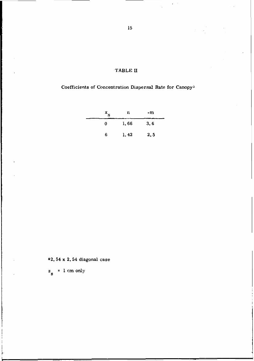
The growth in the characteristic width of the vertical dispersion

of a continuous point source plume has frequently been found to be

proportional to a power function of the longitudinal downstream dis-

ntance, x . Similarly, it is generally observed that the maximum

concentration at ground level decreases at a rate proportional to

x . For a plume dispersing in or above the vegetative canopy, the

rate of dispersal appears to be a function of the fetch distance from

the canopy inception position (see Table II). This marked variation

is evident near the canopy edge as is shown in Figs. 43 and 44.0.7

These rates of dispersion may be compared with values of x and

-1. 5 2x for plumes dispersing over a smooth surface. 20

The nonisotropic character of the horizontal versus vertical

plume dispersal is evident in cross-sections of the plume plotted a

isoconcentration lines (see Figs. 37 to 42). For a source located

15

TABLE [H

Coefficients of Concentration Dispersal Rate for Canopy"

x n -M

0 1.66 3.6

6 1.42 2.5

*2. 54 x 2. 54 diagonal case

zs= I1cm only

16

within the canopy, lateral diffusion is very strong, while for a source

at the top of the canopy, vertical dispersion predominates. Rapid

diffusion in the vertical direction is very evident within the canopy

since gradients in concentration are quickly reduced to a uniform

vertical distribution.

3. Eddy Diffusion Coefficient

The concept of a macroscopic equation of turbulent dispersion

of some property C results generally in the equation

8C + a ) C (K aCat ax. i ax. x. ax.1 1 1 1

where K is the coefficient of turbulent diffusion. The coefficientX.1

K incorporates within itself the complexities of the actual trans-x.1

port process. Hence, most analytical studies of fluid mechanics

require some theoretical or empirical expression for the variation

of Kxi with other parameters. Several scientists have studied the

nature of Kxi for plant communities, but further data are still

needed. 1, 2, 3, 8, 12, 13

The eddy diffusio.a coefficient for transport of the injected gas

in the model canopy has been determined utilizing concentration and

velocity profiles and a finite difference interpretation of Equation (1).

In order to accomplish the calculations with the limited data, it was

assumed that K and K were equal at all levels. Calculations werey z

performed on a CDC 6400 computer at Colorado State UniversityMLI

17

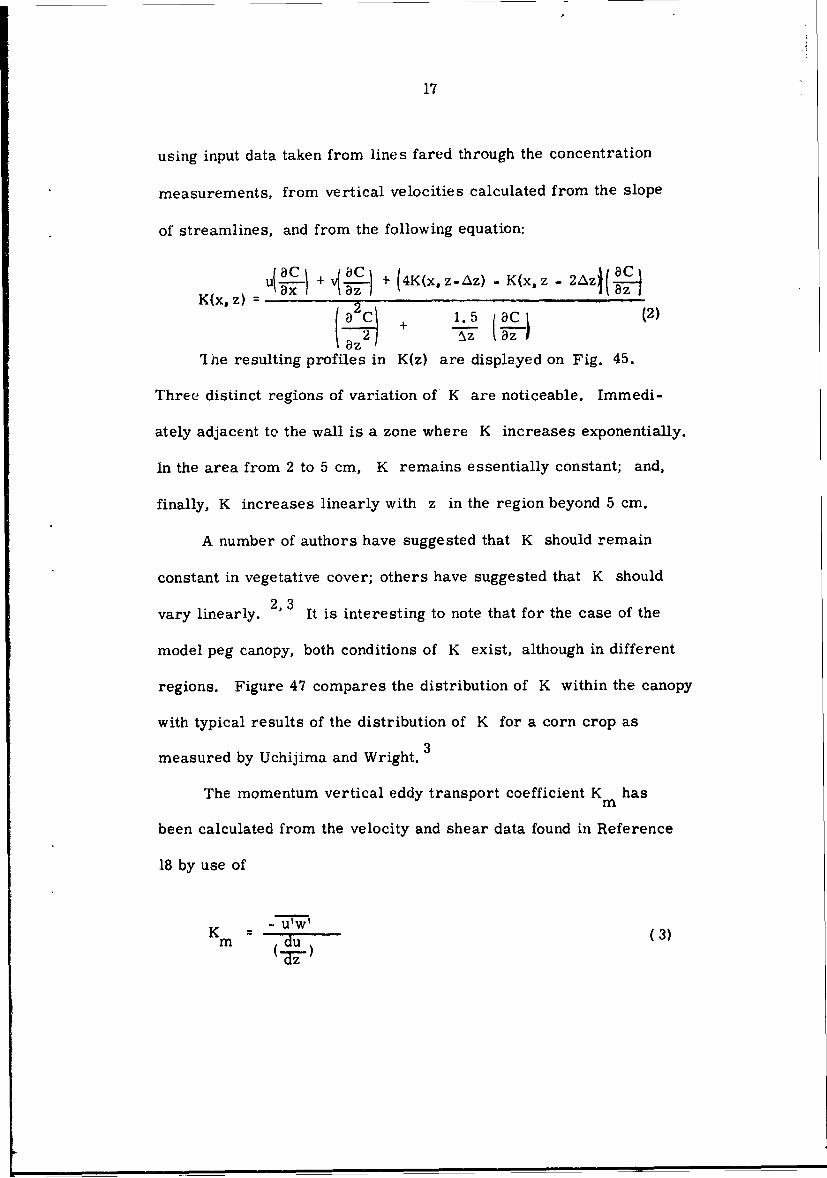
using input data taken from lines fared through the concentration

measurements, from vertical velocities calculated from the slope

of streamlines, and from the following equation:

8C + " + (4K(x. z-Az) -K(x. z -2A+ 'C.K(x, z) 2 (2)

(a2 + 1.5 c 2z , !az 7

Ihe resulting profiles in K(z) are displayed on Fig. 45.

Three distinct regions of variation of K are noticeable. Immedi-

ately adjacent to the wall is a zone where K increases exponentially.

In the area from 2 to 5 cm, K remains essentially constant; and,

finally, K increases linearly with z in the region beyond 5 cm.

A number of authors have suggested that K should remain

constant in vegetative cover; others have suggested that K should

vary linearly. 2,3 It is interesting to note that for the case of the

model peg canopy, both conditions of K exist, although in different

regions. Figure 47 compares the distribution of K within the canopy

with typical results of the distribution of K for a corn crop as

measured by Uchijima and Wright.

The momentum vertical eddy transport coefficient K hasm

been calculated from the velocity and shear data found in Reference

18 by use of

K -(d) (3)

m d

18

Figure 46 compares the variation of the momentum, K and massm

K eddy diffusion coefficients in and above the artificial canopy.c

Above the canopy, K becomes proportional to ( z-d ) where d is

a displacement height. Similar behavior has been observed for

prototype canopies. 1, 2, 3,12,13, 21

As a result of calculations by Denmead, the eddy diffusivity in

a pine forest might also be interpreted to behave in a similar man-21

ner. Wright and Lemon reported K distributions in a canopy of

corn; however, they reported results in terms of a wind profileclassification which does not permit direct comparison. 22 Finally,

these K profiles may also be described as qualitatively similar to

the peg data.

19

CONCLUSIONS

It is apparent that the general character of flow in and above

vegetative canopies may be satisfactorily simulated in the meteorolog-

ical wind tunnel. In addition, these new data suggest that even the

micro-sctucture transport phenomena behave in a manner similar to

that of the prototype. Therefore, it is possible to conclude that:

1) The basic trends of the dynamic and kinematic behavior of a

complex vegetative cover may be simulated by a simple porous

geometry in a wind tunnel.

2) The initial fetch of the peg canopy affects tracer dispersion

of a continuous point source in a unique manner: Vertical convective

motions exhale the gases released at the beginning of the canopy, and

subsequently, the canopy appears to re-inhale the products farther

downstream.

3) The dispersive characteristics of the canopy are non-

isotropic. For a source near ground level, lateral mixing is strong;

for a source located at the top of the canopy, vertical transport

predominates.

4) The eddy diffusion coefficient varies linearly as (z-d)

above a vegetative cover and has a growth rate proportional to ku*.

5) The eddy diffusion coefficient, K , within the artificial

vegetative cover, appears to develop into three regions: Initially K

r20

grows exponentially, next it remains constant, and, finally, K grows

at a linear rate,

6) The experimental law for attenuation of boundary concen-

-2.5tration was obtained as x for gas source releases far from the

canopy inception. (Rates of dispersion are somewhat larger near the

edge of the vegetative cover.)

21

BIBLIOGRAPHY

1. Penman, H. L. and I. F. Long, "Weather in Wheat," Quarterly

Journal of Royal Meteorological Society, Vol. 86, pp. 16-50,1960.

2. Inoue, E., "On the Turbulent Structure of Airflow Within CropCanopies, " Journal of Meteorological Society of Japan, Series11, Vol. 41, #6, December 1963.

3. Uchijima, Z. and J. L. Wright, "An Experimental Study of AirFlow in a Corn Plan-Air Layer, " Bulletin of the NationalInstitute of Agricultural Sciences (Japan), Series A, #11,February 1964.

4. Lemon, E. R., (ed.), "The Energy Budget at the Earth's Surface,"Part II, Production Research Report No. 2, Agricultural ResearchService, U. S. Dept. of Agriculture, 49 p, 1962.

5. Bayton, H. W. "The Penetration and Diffusion of a Fine Aerosolin a Tropical Rain Forest, " Ph. D. Thesis, University ofMichigan, Ann Arbor, 1963.

6. Raynor, G. S., "Effects of a Forest on Particulate Dispersion,USAEC Meteorological Information Meeting, Chalk River,

Canada, September 1967.

7. Plate, E. J. and A. A. Quarishi, "Making of Velocity DistributionsInside and Above Tall Crops, " Journal of Applied Meteorology,Vol. 4, #3, pp. 400-408, June 1965.

8. Yano, Motoaki, " Turbulent Diffusion in a Simulated VegetativeCover, " Fluid Dynamics and Diffusion Laboratory Tech. Rept.CER66MY25, Colorado State University, 1966.

9. Hidy, G. M., (ed), "On Atmospheric Simulation: A Colloquium, I

NCAR Technical Note NCAR-7N-22, Boulder, November 1966.

10. McVehil, G. E., et al., "On the Feasibility of Modeling SmallScale Atmospheric Motions, " Cornell Aeronautical Laboratory,Tech. Rept. ZB-2328-P-1, April 1967.

22

11. Plate, E. J. and J. E. Cermak, "Micro-Meteorological WindTunnel Facility: Description and Characteristics, " FluidDynamics and Diffusion Laboratory, Tech. Rept. CER63EJP-JEC 9, Colorado State University, 1963.

12. Saito, T., "On the Wind Profiles in Plant Communities,"Bulletin of the National Institute of Agricultural Science (Japan),Series A, #11, February 1964.

13. Cionco, R. M., W. D. Ohmstede and J. F. Appleby, "Model forWind Flow in an Idealized Vegetative Canopy, " Report ERT)AA-MET-7-63, Electronics Research and Development Activity,Ft. Huachuca, June 1963.

14. Schlichting, H., Boundary Layer Theory, McGraw Hill Book Co.,Inc., New York, 1960.

15. Tourin, M. H. and W. C. Shen, "Deciduous Forest DiffusionStudy, " Final Report to U. S. Army, Dugway Proving Grounds,Contract DA42-007-AMC-48(R), August 1966.

16. Allison, J. K., L. P. Herrington and J. P. Morton, "DiffusionBelow and Through a Dense, High Canopy, " Paper PRC 68-3,Melpar, Inc., Arlington, Virginia. (Paper presented atConference on Fire and Forest Meteorolgy of the AmericanMeteorological Society and the Society of American Foresters,March 1968.)

17. Hsi, G. and J. H. Nath, "A Laboratory Study on the Drag ForceDistribution Within Model Forest Canopies in Turbulent ShearFlow, " Fluid Dynamics and Diffusion Laboratory Report No.CER67-88GH-JHN-50. Colorado State University. 1968.

18. Kawatani, Takeshi, and R. N. Meroney, "Structure Of CanopyFluid Flow, " Fluid Dynamics and Diffusion Laboratory ]ReportCER67-68TK-RNM-33. Colorado State University. 1968.

19. Jensen. M. and N. Frank. "Model-Scale Test in Turbulent Wind.Part I, " The Danish Technical Press, Copenhagen, 1963.

20. Malhotra, R. C. and J. E. Cermak. 'Mass Diffusion in Neutraland Unstably Stratified Boundary-layer Flows." InternationalJournal of Heat and Mass Transfer. Vol. 7. pp. 169-186. 1964.

23

21. Denmead, 0. T. "Evaporation Sources and Apparent Diffusivitiesin a Forest Canopy, " Applied Meteorology, Vol. 3, pp. 383-389, 1964.

22. Wright, J. L. and E. R. Lemon, "Estimation of TurbulentExchange within a Corn Crop Canopy at Ellis Hollow (Ithaca,N. Y.), 1961," Internal Report 62-7, N. Y. State College ofAgriculture, Cornell University, July 1962.

24

th0

OhlU

25

I I°i, jt-

lii i iiiaII

26

1.0

0.8

0.6

0.4

0.2

0 0.2 0O4 0.6 0.8 1.0

V/ Vh

h HIh

2 - 44.4 0 1.h " h

hLx2 66.7P 83.0

LPegs ~ 0.48 cm, ha9 cm, L a 10.8mn, h a'2 0

Spaced 2.54Kx 2.54cm , V=. 12 rn/s

Fig. 3. Velocity profiles within model canopy

27

x/h1.0- 0 45 ____

o 68a 90 0A 96

0.8 A 106 -__

h:9cn, L =1.8mL :120

01

h0.6 ju

0.4

020

10

Canopy Study: Flow Above CanopyPegs 0 0.48, Spaced 2.54x2.54cm

Fig. 4. Velocity profiles above model canopy

28

an

* 0

00

o 40

0 -0

4a)

04(0U)(n~(D -

w

0, 0

(W)0HG

29

EEu 0

0

CL w,

I 0

0 0

(WO) 1HO13H

1 30

'0

C C

E E00 o q

o d O, tflIf If It 11 is 0w

00

w -0.)

0

0

I 0.

Cd

00

CVl

~W3 z

31

0

0

0 0

'o 0

CU

CL CU

MCZU

,4

0

0 0 0 0

). 01HO13

32

50004

0 0.3 m FROM SOURCE4000 0 o .61 M

6 0.91m

S h--

3000 _

I* o aPEGS:.o'.4cm, h9c, L.IOm, o120

2 ISPACED 2.54 x 2.54 cm

20(: ' ' I Z," Icm

2000- , X.Om

.. .. \ \ ,.

1000

0 5 10 z(cm) 20

Fig. 9. Vertical dispersion of a continuous point source in a modelpeg canopy(2.54x2.54cm). xs 0, z s 1 cm

A,_

33

0LY _ _ _ _ _ _ in

Is Ni

2C

0

0 0

ffC)

00 0

In x

NL v

000 0 0

9-01.0

j 34

00

35

In CIn

N 0

ww

0 -4=0 0c

W 0

0_0-

EE

0-

9~ 0,,.

0

04

Ina

36

-0

MU E

kn V ;

E NEIi- C0r E

E E S. N x

g o _ _ _ _ _ _ _

______ ___/_0000/x~

SQQ

37

0.

LRI to_ - _

N l 0.CL

E (DEA CM

000

iv C~C

oN

14'

0u*~OI to

38

* °

uO0000

C

_. ° °oO O O , , . ' I/ o

0

/Ii i i.-

C m l

:!/~~ 04 / ,

I/, EEE

/0 -- o

N000 4 It

0 4~

- - ~N C O

40J U C

-U)

- 0

4C

Q tN

-~ LL9 ~OI X

39

301o 2.54

& 5.08

£ 1016

o 15.24

* 20.32

Pegs: 0 =O.48, hz 9cm, La 10.8L /h 120, Spaced: 2.54x2.54cm

xS: 6m

x=0.3mVw :12 mAec

Fig. 16. Lateral dispersion of a continuous point source ina model peg canopy (2. 54 x 2. 54 cm). xs 6 m,z = h

s

J 40

E

0

CD in

0

c( U

u 0r

00

Oe.1 114o oI9 N -W

1 -.

21000N -U0

lel'-4

41

G -T6

300 2"0

4"6"1

A i'

200

100

051015 2025 30

Fig.18.Lateral dispersion of a continuous point source ina model peg canopy (2. 54 x 2. 54 cm). x s=6 m,z ~h

SPEGS: #0.486~m, h =9cm, L 10,8m, 12, SPACED 2.54x 2,54cm

ZS =h 0,3m FROM SOURCE

Vw 12 rn/sec

1 42

8 0

-4

0

o cd

6I 0

ow

0.

LO'-

C9

0)

N0

43

T

EE E E E 0

@400 ' ~0S.'

L -0ie 2

02

co 0

0 0

010

EU .EIvN >

6cU 44

j 44

4~F 0 C

N~ .)

T -

0

0

oD r r,0) 0

E7 00

EU E

-4

45

0d

0

C'CU

N i N

x

Cd

0

0 m

o i

o coCd

0 04 * )

00

4 0C D N a D 05IDq N 0

d 46

ti

0

Cd

0.

0E

(U

E 0E 0.E0

CY C0

0

04

*X

0.

0400 0 ~Lc

I 1 1 E

00

47

0.

00

4. - N

r4a

4 0

0

CO

0.

0Y 0oa~0 0

in C

OoC

49

0.

0

00

0

on.' 0~ vEEE

£000

.00

-8-

9-01

>zo

0000

N' o.,

0 i" 0 Cd .0 C.00

o O"1 * @4

0 Ia

-4

E 0 If

co 4aoIf 0 z

u ui 0

C5 4-0

E C:

w CL " 4AIf ) uoNN

o.

0 0

C)

In

41 o)

9.01 X 0

E

U)-f

x N)

Q)

0

0

Sd0S4

41-

I-I

0

CL 0

cj N

<

N QN

U) U0N

10

In.

o 0

0

W Cdz0

w 0

OL-

0 0-0co

Joo

-~ N N

N1

E x

cn 0

00

0 -

00

0

4

I N %

-A0N E N N N N N V C) ~N

-ICY

0 0

('300

.2

"0

060

Zto0 L4J

11 0

x 21%

0 3 I

cli coOD C ~ OD WCs. CN N -- -

55

ci

(d

000

0~C4

-4

WC.'

-IY x

00 i

-I IN

C-ICUNOD I- E L

0tv

CLC

U

41

0h

II

NN

EE

E E E *.K q

000

00

n.

W~~A N O $ N .

N 0~~~u 0

12

0

N (A

UT,

0 0 00

In E

0 u0

it,

0 tv

10

0E

I ) cn

I I U-I--I--I----to

~~~1~ 0

0 E

o fl E

_ E

0.4 0t w a.

LA 0EEr

<a.N(

61

E

CY(1 (MJ

010

c~ EOC) *0 X 4

10 ~~ ~ w k E

~C)

N N12

C\)c

0 O

tn"-4

62

z(CM)26

24 Z =Icm

221 x = 0.2 5m

20 Pegs- 4S =0.48cm, h =9cm

18 Spaced: 2.54 x2.54 cm Diagonally

16

124

10

0 2 4 6 8 10 12 14 16 18 20 22 24 26y (cm)

Fig. 39. Gaseous plume cross-section of a continuous point sourcein a model peg canopy (2. 54 x 2. 54 cm diagonal). x s=6 m,z s =1 cm, x =0. 25 m

63

z

30 x =6 m

28 -c

26- Pegs: (P =0.48 CM, h 9 cm

24 -Spaced: 3.60 x360 cm(Diagonally)

22

20i/8

16

12

8

6

4

2

0 -o 2 4 6 8 10 12 14 16 18 20 22 24 26y (cm)

Fig. 40. Gaseous plume cross-section of a continuous pointsource in a model peg canopy (2. 54 x 2. 54 cmdiagonal). 'x s ~6m, zs =h, x =0. 5m

64

3.75Pegs*~0.48cm, hz9cm

Spaced& 5.08 x 5.08 cm

E0 900 I8 C 2

0 800 10 8 =2

0 1.25 2.50 3.75 5.00Y (cm)

Fig. 41. Gaseous plume cross-section of a continuous pointsource in a model peg canopy (5. 08 x 5. 08 cm).xs =0 m, z s= I1cm, x=O0.3 m

65

____ ___ _ _ ___ ___ __ ___ ___ IA) a)I . E0

004

Q) AZ

U 0~0 000

(rD

4

-4 0

0 7)L

-4 C

,Ik,

66

KJ x$_ O z_ lc \oS0

0

0

-3.70 x5 :0 ,zszIcm0 0 , 4.5cm Spacing -- -- __--

A 6m, Icm 2.54x2.54

a 6m, 4.5cm Diagonal

A 6m, 9cm m-- -2.5

0 6m, Icm Spacing2.54x2.54

01 110 0x (meters)

Fig. 43. 'variation of ground level concentration withdownstream distance

Pegs 0.48cm, h'9cm

67

00

0Q00

co

00

4J

00

- 4

B co

E E0~.o U

* * 02

coto :>

C~i C)%-

l.

0Nv

(W)409iH OWfl~d O!Isl!JB:DJD4:3

68

28-

24-

- 00

20-

- 00

a0

160 0

0 0

12- a 0

a 0

S a /0 xs,6m zs--Icm

0 0 A }XO.'5m 254x2.54 cma xi %6m

8- o x0l0m DIOQonlI %Or x} zI cm

a 0 A x,.6m 2.54x2.54cmD A O

• 4- o0oo

0 0.2 0.4 0.6 0.8 10K€ (m2/Ac)

Fig. 45. Coefficient of turbulent diffusion

69

0

w 0\

a U 0E0

enOe

Ch

F.- E 0

0 0

00in7N AC

70

E

, E

E E E E. 3

_. Ow§

0 1 1 ; 11 I

VC x x 41

h~N5E

o 00

E E.

Ow-

*4en

UnclassifiedSecivrity Classification

DOCUMENT CONTROL DATA - R&D(Security class iItcoition of lI to. bidy of abatrac I and indexing annsiouoion mu at be entered when the ove rat l report aca o i

Ig tjrNA1 ACJIJIU J(Cirport uho) 28 REPORT SECURITY CLASSIFCAIONC ta nivesityUnclassified

Foothills Campus 26GRUFort Collins, Colorado 80521

3 flEPORT TITLE

"GASEOUS PLUME DIFFUSION CHARACTERISTICS WITHIN MODELPEG CANOPIES"

4 OESCRIPTIVE NOTES (7yp, of report and inclusive data*)

Technical Report5 AUTHOR(S) (Lost name. iftt name. Initial)

Meroney, R. N.; Kesic, D.; and Yamada, T.

6 REPORT DATE 7. TOTAL NO OF PAGES -76 NO OF REFS

KJuly, 1968 71 22$40 CONTRACT OR S0RANT No. 90 ORIGINATOR'S REPORT NUMISOERS)

UAAbO7-68-C-04 23 CER68-69RNM- DK-TY-3b. PROJECT NO0.

2275C, 36. OTpHER wREPORT No(S) (Anv other numbers Ael ay I-oesno

ohs$ report)

* d

010 A VAIL ABILITY'ILIUITATiON NOTICES

Distribution of this report is unlimited

I I SUPPL EMCNTARY NOTES 123 SPONSORINkG MILITARY ACTIVITY

U. S. Army Materiel Command

13 ABTRACTA point source of an air-helium mixture was releasedcontinuously at various positions within a simulated canopy composed of9 cm high pegs. 0. 48 cm diameter, spaced in several arrays (2. 54 x 2. 54,3. 55 x 3. 55, and 5.08 x 5.08 cm). Variations of the vertical location of thesoarce revealed the strongly nonisotropic character of diffusion within acanopy with respect to the relative diffusioai rates in the lateral and verticaldirections. When the source was placed at various downstream distancesfrom the edge of the canopy, it displayed a tendency to exhale the plume nearthe frunt of the model canopy and to inhale the plume at distances furtherdownstream. Calculations of the turbulent diffusion coefficient, K to withinand above the canopy from the experimental data. reveal both a constantregion and a region of linear increase with height mnrase as suggested byprevious authors.

D D "?.14 73 UnclassifiedCasfclo

Unclassified

4 LINK A LINK B LINK C

ROL E I Rt OL. 1 OE "

Simulatk.onAtmospheric Modeling

Wind-Tunnel LaboratoryTurbulent FlowDiffusionFluid MechanicsMicr . eteorologyForest MeteorologyVegetative Canopies

INSTRUCTIONS

1. ORIGINATING ACTIVITY: Enter the name and address 10. AVAILADILITY/LIMITATION NOTICES: Enter any lint-of the ccntractor, subcontractor, grantee, Department of De- ftat ions on further dissemination of the report. other than thosefense actlvit7 or other organization (corporate author) issuing i y classification usi"g standard statementsthe report. such as:

2a. REPORT SECUIRTY CLASSIFICATION: Enter the over- (1) "0uilied requesters may obtain copies of thisall security classification of the reporl. Indicate whether report from DDC.""Restricted Data" is included. Marking is to be in accord-ance with appropriate security regulations. (2) "Foreign announcement and dissemination of this

2b. GROUP: Automatic downgrading is specified in DOD Di- repor by DC is not authorized."rective 5200. 10 and Armed Forces Industrial Manual. Enter (3) "U. S. Gcvernment agencies may obtain copies ofthe group number. Also. when applicable, show that optional this report directly from DDC. Other qualified DDCmarkings have been used for Group 3 and Group 4 as author- users shall request throughized.

3. REPORT TITLE: Enter the complete report title in all (4) "J. S. niitary agencies may obtain copies of thiscapital letters. Titles in all cases should be unclassified. report directly from DDC. Other quaified usersIf a meaningful title cannot be selected without classifica- shall request throughtion, show title classification in all capitals in parenthesis ,immediately following the title. .__

4. DESCRIPTIVE NOTES. If appropriate, enter the type of (5) "All distribution of this report is controlled. Qual-report, e.g., interim, progress, summary, annual, or final. ified DDC i:3ers shall request throughGive the inclusive dates when a specific reporting period is ,"covered.

If the report has been furnished to the Office of Technical5. AUTHOR(S): Enter the name(s) of autho(s) as shown on Services. Department of Commerce, for sale to the public, indi-or in the report. Enter last nare, first name, middle initial. cate this fact and enter the price, if known.If military, show rank and branch of service. The name of Ithe principal author is an absolute minimum requirement. 11. SUPPLEMENTARY NOTES: Use for additional explana-

6. REPORT DATE: Enter the date of the report as day, tory notes.

month, year; or month, year, If more than one date appears 12. SPONSORING MILITARY ACTIVITY: Enter the name ofon the report, -,se date of publication, the departmental project office or laboratory sponsoring (pay-

7.. TOTAL NUMBER OF PAGES: The total page count ing for) the research and development. Include address.

should follow normal paginaiion procedures, i.e., enter the 13. ABSTRACT: Enter an abstract giving a brief and factualnumber of pages containing information. summary of the document indicative of the report, even though

it may alsi(- appear elsewhere in the body of the technical re-7b. NUMBER OF REFERENCES: Enter he total number of port. If additional space is required, a continuation sheetreferences cited in the report. shall be attached.

go. CONTRACT OR GRANT NUMBER: If appropriate, enter It is highly desirable that the abstract of classified re-the applicable number of the contract or grant under which ports he unclassifi,,d. Eac-h paragraph of the abstract shallthe report was written. end with an indication of the military security classification

8b. 8c, & 8d. PROJECT NUMBER: Enter the appropriate of the information in the paragraph, represented as (TS), (S).

military department identification, such as project number, (C), o (U).

subproject -:umber, ". ,item numbers, task number, etc. There is no limitation on the length of the abstract. How-

9a. ORIGINATOR'b REPORT NUMBER(S): Enter the offi- ever, the suggested length is from 150 to 225 words.

cial report number by which the document will be identifiod 14. KEY WORDS: Key words are technically meaningful termsand controlled by the originating activity. This number must or short phrases that characterize a report and may be used asbe unique to this report, index entries for cataloging the report. Key words must be

qb. OTHER REPORT NUMBER(S): If the report has been selected so that no security classification is required. Iden-

assigned any other report numbers (either ki the originator fiers, such as equipment model designation, trade name, itili-

or by the sponsor), also enter this number(s), tarv project code name, geographic location, may be used askey wnrds hut will he followed bV an indication of t. hnicalcontext. The assignment of links, rules, and weights isoptional.

Unclassified