by Michail Famelis - WordPress.com · Michail Famelis Doctor of Philosophy ... Yuval Filmus, and...
180
Managing Design-Time Uncertainty in Software Models by Michail Famelis A thesis submitted in conformity with the requirements for the degree of Doctor of Philosophy Graduate Department of Computer Science University of Toronto c Copyright 2016 by Michail Famelis
Transcript of by Michail Famelis - WordPress.com · Michail Famelis Doctor of Philosophy ... Yuval Filmus, and...

Managing Design-Time Uncertainty in Software Models
by
Michail Famelis
A thesis submitted in conformity with the requirementsfor the degree of Doctor of Philosophy
Graduate Department of Computer ScienceUniversity of Toronto
c© Copyright 2016 by Michail Famelis

Abstract
Managing Design-Time Uncertainty in Software Models
Michail Famelis
Doctor of Philosophy
Graduate Department of Computer Science
University of Toronto
2016
The concern for handling uncertainty in software pervades contemporary software engineering. A par-
ticular form of uncertainty is that which can exist at multiple stages of the development process, where
developers are uncertain about the content of their artifacts. However, existing tools and methodologies
do not support working in the presence of design-time uncertainty, i.e., uncertainty that developers have
about the content of their artifacts in various stages of the development process, therefore having to
mentally keep track of multitude of possible alternative designs. Because of this uncertainty, developers
are forced to either refrain from using their tools until uncertainty is resolved, or to make provisional
decisions and attempt to keep track of them in case they prove premature and need to be undone. These
options lead to either under-utilization of resources or potentially costly re-engineering.
This thesis presents a way to avoid these pitfalls by managing uncertainty in a systematic way. We
propose to to work in the presence of uncertainty and to only resolve it when enough information is
available. Development can therefore continue while avoiding premature design commitments.
In a pilot user study we found that, when asked to articulate design-time uncertainty in a free-
form modelling scenario, people tend to explicate it within the software artifact itself, staying close
to the existing notation. This lead us to adopt “partial models”, a formalism for representing sets of
possible design alternatives while staying faithful to the underlying language. This way, the problem of
managing uncertainty in software artifacts is turned into a problem of doing management of software
artifacts that contain uncertainty. To manage partial models, we have thus leveraged several software
engineering sub-disciplines to develop techniques for: (a) articulating uncertainty, (b) checking and
enforcing properties, as well as generating appropriate user feedback, (c) applying transformations, and
(d) systematically making decisions, as new information becomes available. The resulting partial model
management framework utilizes novel abstraction and automation approaches and enables a principled
and systematic approach to managing design-time uncertainty in the software development process.
ii

To Natalie.
iii

Acknowledgements
It has been an immense privilege and honour to apprentice with Marsha Chechik. Her mentorship,
example, guidance, support and teaching has profoundly transformed me in more ways that one. From
her I learned how to be a scientist, a writer, a researcher, an editor, a manager, a member of the academic
community, a mentor, a planner, a communicator, a reviewer, a coordinator, and even a little bit of a
salesperson. Marsha has taught me to aspire to be demanding and fair, fierce and gentle, reliable and
uncompromising, direct and subtle. Or, as Natalie put it, to aspire to “be the Marsha I want to see in
the world”.
I have also been privileged to work closely with Rick Salay. He was always willing to put in the extra
effort to explain difficult mathematical concepts to me, discuss my wildest research ideas and help me
develop my skills in formal specification and reasoning. In some ways, I feel like Rick Salay has been
almost like a co-supervisor to me.
I also thank Alessio Di Sandro for all the hard engineering work he put into Mu-Mmint. Without
his titanic efforts much of what is described in this thesis would be just symbols on paper. Alessio has
also been a great friend and I thoroughly enjoyed our chats about all the ways our continent of origin is
suffering.
I am deeply grateful to people who gave me feedback and commented on my thesis. Specifically, I
thank the people who were in my supervisory and examination committee: Steve Easterbrook, Renee
Miller, Carlo Ghezzi, and Kelly Lyons. Their comments really helped clarify and solidify my thoughts
about the concepts discussed in the thesis. The ideas and concepts in it would not be as clear without
them. Also, over the years I received critical feedback which greatly helped me, for which I want
to specifically thank: Reviewer #2 of the TOSEM manuscript Towards Modeling and Reasoning with
Design-Time Uncertainty, Krzysztof Czarnecki, Benoit Baudry, Greg Wilson, Fabiano Dalpiaz, and Jordi
Cabot.
I also wish to thank my collaborators and co-authors, whose contributions helped shape this thesis:
Stephanie Santosa, Julia Rubin, Levi Lucio, Naama Ben-David, Ahmed Mashiyat, Gehan Selim, Pooya
Saadatpanah, Jan Gorzny, Shoham Ben-David, Nathan Robinson, James R Cordy, Juergen Dingel,
Hans Vangheluwe, Ramesh S, Sahar Kokaly, Vivien Suen, Oloruntobi Ogunbiyi, Qiyu Zhu, and Kawin
Ethayarajh.
I am also very lucky to have had excellent colleagues whose friendship, and camaraderie helped me
grow as a person and as an academic. Aws Albarghouthi was a great friend and many times an inspira-
tion for his efficiency and clarity of vision. Jocelyn Simmonds taught me how to get over the impostor
syndrome and showed me how to navigate the academic space, building my confidence in my own capa-
bilities in the process. Alicia Grubb taught me many things, most crucially to examine critically my own
conduct and behaviour. I am also very grateful for the companionship, camaraderie and friendship of
the many people I was lucky to meet and work side by side with through my years at U of T: Albert An-
gel, Anya Tafliovich, Apostolos Dimitromanolakis, Benson Quach, Christina Christodoulakis, Elizabeth
Patitsas, Foteini Agrafioti, George Amvrosiadis, Golnaz Elahi, Jennifer Horkoff, Jorge Aranda, Manos
Papaggelis, Maria Attarian, Maria Kyriakaki, Maria Pavlou, Marios Fokaefs, Michael Mathioudakis,
Nan Niu, Neil Ernst, Nikos Anesiadis, Petros Spachos, Sotiris Liaskos, Tasos Zouzias, Yannis Prassas,
Yannis Sakellaridis, Yannis Sarkas, Yi Li, Yuval Filmus, and Zak Kincaid.
A doctorate is almost by definition a long and arduous process that has no guarantee of success. I
am grateful to Steve Rutchinski and Marina Haloulos who made it administratively possible for me to
iv

not drop out due to poor financial planning on my part. Additionally, I am thankful to Solomon Shapiro
from the university’s Counselling and Psychological Services, as well as the facilitators and participants
at the B-Side workshop for helping me remain a balanced individual who is at peace with myself.
For their invaluable financial support that was so much needed at the very start of my studies, I
am especially thankful to Kostas Stamatakis, Manolis Giakoumakis, and fr. Gavriil Tsafos. Kostas
Stamatakis and Maria Pavlaki are responsible for the fact that, growing up, I always took for granted
that I would do a PhD. However, as a fledgling undergraduate student, I would not have even made to
graduate school if it was not for Kostas Kontogiannis, and Nikos Papaspyrou, professors at the National
Technical University of Athens, who inspired and mentored me in crucial points of my intellectual
development.
My time in graduate school coincides with the economic, social, and political crisis in Greece. I
thus also want to especially thank the people who, either through the Greek Solidarity Initiative or the
Greek Canadian Democratic Organization, helped me to constructively channel my concerns, worries,
fears and hopes into meaningful political action: Dimitris Apostolopoulos, Nikos Gryspolakis, Yannis
Angelopoulos, Tasos Dimopoulos, Platon Routis, Anna Kostouki, Dionysos Savopoulos, Antonis Batsos,
and Penny Siganou.
In Rhythms of Resistance – Toronto, I found community, friendship, wisdom, strength, resilience, cre-
ativity, music, affection, acceptance, and an uncompromising desire to be better, more loving, more open,
more accepting, more aware, more alive. I feel truly privileged to have played, marched, partied, argued,
relaxed, sung, danced, eaten and co-conspired with all the RoR bandies: Amelia Murphy-Beaudoin, An-
drea Albagli, Angela Woodcock, Anjali Helferty, Ayelit Gabler, Bonnie Briggs, Dave Campanella, Eliz-
abeth Patitsas, Gary Pereira, Jamie Smith, Jesse Ovadia, Jonnie Bakan, Kelsy Vivash, Kuba Borowiec,
Laura Severinac, Mary Lindsay, Melissa McKechnie, Natalie Mathieson, Olga Parysek, Sarah Michael,
Steph McKechnie, Timothy Luchies, Yuval Filmus, Zak Smith, and Zena Lord. I am especially thankful
and appreciative to the four wise women of the “power circle”: Katelyn Blascik, Laura Hartley, Cate
Ahrens, and, of course, Natalie. They literally changed my life forever.
When I first came to Canada I did not expect to also find an adoptive family. The Caines and
the Tuddenhams took me in me as their own. Annette, Michael, Barbara, Jean, Ardwell, Joyce, Matt,
Alexandra, Sydney, Travis, Kara, Hannah, Jay, Liam, Jeff, Elizabeth, thank you for the warmth, accep-
tance, and affection with which you embraced me.
My siblings Marietta, Panagiota, and Panagiotis, thank you for all your love, support and under-
standing! Thank you for accepting me for myself and for being a lifeline to my roots. My parents
Giorgos, Polymnia, thank you for ...everything. Thank you for the small things: for all the hours that
you spent listening to me rambling on the phone, for cheering me on, for telling me news from home, for
passing my greetings to friends and family, for sending me money when I needed it, for the household
survival tips, for holding on to me: Dimitris Karagiannis once told me that listening to you talk about
me felt as if I had never left Greece. And thank you for the big things: for my nurturing and upbringing,
for freeing me to choose my path and giving me the space to pursue it. Thank you for trusting me with
your hopes and your dreams. Thank you for all the sacrifices you made. As a parent, I now think I am
beginning to understand just how hard my absence has been for you. I know you are very proud of me.
I know you would be very proud of me regardless of how this adventure would have concluded.
Yuri, thank you for making everything urgent. You are my thesis baby and all of this would probably
not be finished on time without you.
v

Most of all, I am thankful to and for Natalie Caine, my companion, accomplice, friend, partner and
love. First of all, thank you for your patience. Thank you for your love and acceptance. Thank you
for your emotional and intellectual support. Thank you for your strength and your wisdom. Thank
you for making me see things in different ways, for opening my eyes to my own self, for educating and
critiquing me. Thank you for your not-so-well-hidden labour: thank you for all the times you cooked
for me, cleaned for me, tidied up for me, did my laundry, made the beds, did the shopping, kept track
of things, organized our outings, kept the baby, made sure I was surrounded by the routine I needed to
focus. Thank you for letting me pull all-nighters and thank you for letting me vegetate to recover from
them. Thank you for insisting we go for walks: you were always right. Thank you for insisting I did
not quit. Thank you for helping me quit smoking. Thank you for our child. This would not have been
possible without you. Now it is my turn to nurture your dreams. At least, I guarantee you, you will
never have to hear the dreaded phrase “I have to work on my thesis” ever again.
vi
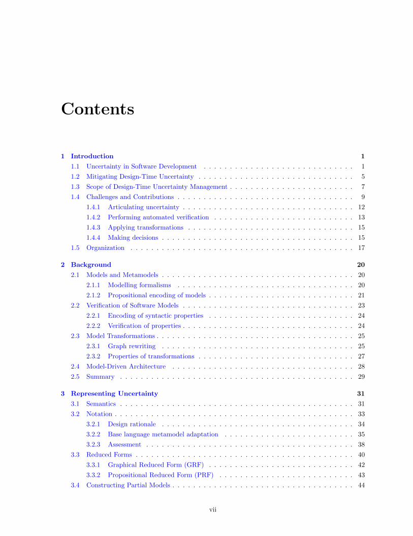
Contents
1 Introduction 1
1.1 Uncertainty in Software Development . . . . . . . . . . . . . . . . . . . . . . . . . . . . . 1
1.2 Mitigating Design-Time Uncertainty . . . . . . . . . . . . . . . . . . . . . . . . . . . . . . 5
1.3 Scope of Design-Time Uncertainty Management . . . . . . . . . . . . . . . . . . . . . . . . 7
1.4 Challenges and Contributions . . . . . . . . . . . . . . . . . . . . . . . . . . . . . . . . . . 9
1.4.1 Articulating uncertainty . . . . . . . . . . . . . . . . . . . . . . . . . . . . . . . . . 12
1.4.2 Performing automated verification . . . . . . . . . . . . . . . . . . . . . . . . . . . 13
1.4.3 Applying transformations . . . . . . . . . . . . . . . . . . . . . . . . . . . . . . . . 15
1.4.4 Making decisions . . . . . . . . . . . . . . . . . . . . . . . . . . . . . . . . . . . . . 15
1.5 Organization . . . . . . . . . . . . . . . . . . . . . . . . . . . . . . . . . . . . . . . . . . . 17
2 Background 20
2.1 Models and Metamodels . . . . . . . . . . . . . . . . . . . . . . . . . . . . . . . . . . . . . 20
2.1.1 Modelling formalisms . . . . . . . . . . . . . . . . . . . . . . . . . . . . . . . . . . 20
2.1.2 Propositional encoding of models . . . . . . . . . . . . . . . . . . . . . . . . . . . . 21
2.2 Verification of Software Models . . . . . . . . . . . . . . . . . . . . . . . . . . . . . . . . . 23
2.2.1 Encoding of syntactic properties . . . . . . . . . . . . . . . . . . . . . . . . . . . . 24
2.2.2 Verification of properties . . . . . . . . . . . . . . . . . . . . . . . . . . . . . . . . . 24
2.3 Model Transformations . . . . . . . . . . . . . . . . . . . . . . . . . . . . . . . . . . . . . . 25
2.3.1 Graph rewriting . . . . . . . . . . . . . . . . . . . . . . . . . . . . . . . . . . . . . 25
2.3.2 Properties of transformations . . . . . . . . . . . . . . . . . . . . . . . . . . . . . . 27
2.4 Model-Driven Architecture . . . . . . . . . . . . . . . . . . . . . . . . . . . . . . . . . . . 28
2.5 Summary . . . . . . . . . . . . . . . . . . . . . . . . . . . . . . . . . . . . . . . . . . . . . 29
3 Representing Uncertainty 31
3.1 Semantics . . . . . . . . . . . . . . . . . . . . . . . . . . . . . . . . . . . . . . . . . . . . . 31
3.2 Notation . . . . . . . . . . . . . . . . . . . . . . . . . . . . . . . . . . . . . . . . . . . . . . 33
3.2.1 Design rationale . . . . . . . . . . . . . . . . . . . . . . . . . . . . . . . . . . . . . 34
3.2.2 Base language metamodel adaptation . . . . . . . . . . . . . . . . . . . . . . . . . 35
3.2.3 Assessment . . . . . . . . . . . . . . . . . . . . . . . . . . . . . . . . . . . . . . . . 38
3.3 Reduced Forms . . . . . . . . . . . . . . . . . . . . . . . . . . . . . . . . . . . . . . . . . . 40
3.3.1 Graphical Reduced Form (GRF) . . . . . . . . . . . . . . . . . . . . . . . . . . . . 42
3.3.2 Propositional Reduced Form (PRF) . . . . . . . . . . . . . . . . . . . . . . . . . . 43
3.4 Constructing Partial Models . . . . . . . . . . . . . . . . . . . . . . . . . . . . . . . . . . . 44
vii

3.5 Related Work . . . . . . . . . . . . . . . . . . . . . . . . . . . . . . . . . . . . . . . . . . . 45
3.5.1 Metamodels . . . . . . . . . . . . . . . . . . . . . . . . . . . . . . . . . . . . . . . . 45
3.5.2 Partial behavioural models . . . . . . . . . . . . . . . . . . . . . . . . . . . . . . . 45
3.5.3 Software product lines . . . . . . . . . . . . . . . . . . . . . . . . . . . . . . . . . . 46
3.6 Summary . . . . . . . . . . . . . . . . . . . . . . . . . . . . . . . . . . . . . . . . . . . . . 48
4 Reasoning in the Presence of Uncertainty 50
4.1 Checking Properties of Partial Models . . . . . . . . . . . . . . . . . . . . . . . . . . . . . 51
4.1.1 Verification semantics . . . . . . . . . . . . . . . . . . . . . . . . . . . . . . . . . . 51
4.1.2 Decision procedure . . . . . . . . . . . . . . . . . . . . . . . . . . . . . . . . . . . . 52
4.2 Generating Feedback . . . . . . . . . . . . . . . . . . . . . . . . . . . . . . . . . . . . . . . 53
4.2.1 Generating a counter-example . . . . . . . . . . . . . . . . . . . . . . . . . . . . . . 53
4.2.2 Generating an example . . . . . . . . . . . . . . . . . . . . . . . . . . . . . . . . . 54
4.2.3 Generating a Diagnostic Core . . . . . . . . . . . . . . . . . . . . . . . . . . . . . . 54
4.3 Experimental Evaluation . . . . . . . . . . . . . . . . . . . . . . . . . . . . . . . . . . . . . 54
4.3.1 Experimental setup . . . . . . . . . . . . . . . . . . . . . . . . . . . . . . . . . . . . 55
4.3.2 Experimental inputs . . . . . . . . . . . . . . . . . . . . . . . . . . . . . . . . . . . 55
4.3.3 Implementation . . . . . . . . . . . . . . . . . . . . . . . . . . . . . . . . . . . . . . 56
4.3.4 Methodology . . . . . . . . . . . . . . . . . . . . . . . . . . . . . . . . . . . . . . . 57
4.3.5 Results . . . . . . . . . . . . . . . . . . . . . . . . . . . . . . . . . . . . . . . . . . 57
4.3.6 Threats to validity . . . . . . . . . . . . . . . . . . . . . . . . . . . . . . . . . . . . 60
4.4 Related Work . . . . . . . . . . . . . . . . . . . . . . . . . . . . . . . . . . . . . . . . . . . 60
4.5 Summary . . . . . . . . . . . . . . . . . . . . . . . . . . . . . . . . . . . . . . . . . . . . . 61
5 Transforming Models Containing Uncertainty 63
5.1 Intuition of Lifting . . . . . . . . . . . . . . . . . . . . . . . . . . . . . . . . . . . . . . . . 63
5.2 Lifting Algorithm . . . . . . . . . . . . . . . . . . . . . . . . . . . . . . . . . . . . . . . . . 65
5.2.1 Specification of lifting . . . . . . . . . . . . . . . . . . . . . . . . . . . . . . . . . . 66
5.2.2 Lifting example . . . . . . . . . . . . . . . . . . . . . . . . . . . . . . . . . . . . . . 66
5.2.3 General case . . . . . . . . . . . . . . . . . . . . . . . . . . . . . . . . . . . . . . . 68
5.2.4 Correctness . . . . . . . . . . . . . . . . . . . . . . . . . . . . . . . . . . . . . . . . 69
5.3 Properties of Lifted Transformations . . . . . . . . . . . . . . . . . . . . . . . . . . . . . . 70
5.3.1 Termination . . . . . . . . . . . . . . . . . . . . . . . . . . . . . . . . . . . . . . . . 70
5.3.2 Confluence . . . . . . . . . . . . . . . . . . . . . . . . . . . . . . . . . . . . . . . . 71
5.4 Evaluation . . . . . . . . . . . . . . . . . . . . . . . . . . . . . . . . . . . . . . . . . . . . . 71
5.5 Related Work . . . . . . . . . . . . . . . . . . . . . . . . . . . . . . . . . . . . . . . . . . . 72
5.6 Summary . . . . . . . . . . . . . . . . . . . . . . . . . . . . . . . . . . . . . . . . . . . . . 73
6 Removing and Resolving Uncertainty 74
6.1 Uncertainty-Removing Refinement . . . . . . . . . . . . . . . . . . . . . . . . . . . . . . . 75
6.1.1 Manual decision making . . . . . . . . . . . . . . . . . . . . . . . . . . . . . . . . . 75
6.1.2 Property-driven refinement . . . . . . . . . . . . . . . . . . . . . . . . . . . . . . . 77
6.2 Experimental Study of Property-driven Refinement . . . . . . . . . . . . . . . . . . . . . . 78
6.2.1 Experimental setup . . . . . . . . . . . . . . . . . . . . . . . . . . . . . . . . . . . . 78
viii

6.2.2 Inputs, implementation and methodology . . . . . . . . . . . . . . . . . . . . . . . 79
6.2.3 Results . . . . . . . . . . . . . . . . . . . . . . . . . . . . . . . . . . . . . . . . . . 79
6.3 Related Work . . . . . . . . . . . . . . . . . . . . . . . . . . . . . . . . . . . . . . . . . . . 81
6.4 Summary . . . . . . . . . . . . . . . . . . . . . . . . . . . . . . . . . . . . . . . . . . . . . 82
7 A Methodology for Uncertainty Management 83
7.1 The Uncertainty Waterfall . . . . . . . . . . . . . . . . . . . . . . . . . . . . . . . . . . . . 83
7.2 Uncertainty Management Operators . . . . . . . . . . . . . . . . . . . . . . . . . . . . . . 86
7.2.1 Articulation stage . . . . . . . . . . . . . . . . . . . . . . . . . . . . . . . . . . . . 87
7.2.2 Deferral stage . . . . . . . . . . . . . . . . . . . . . . . . . . . . . . . . . . . . . . . 88
7.2.3 Resolution stage . . . . . . . . . . . . . . . . . . . . . . . . . . . . . . . . . . . . . 89
7.3 Application: Uncertainty Management in MDA . . . . . . . . . . . . . . . . . . . . . . . . 92
7.4 Tool Support . . . . . . . . . . . . . . . . . . . . . . . . . . . . . . . . . . . . . . . . . . . 96
7.5 Related Work . . . . . . . . . . . . . . . . . . . . . . . . . . . . . . . . . . . . . . . . . . . 99
7.6 Summary . . . . . . . . . . . . . . . . . . . . . . . . . . . . . . . . . . . . . . . . . . . . . 101
8 Worked-Out Examples 102
8.1 UMLet Bug #10 . . . . . . . . . . . . . . . . . . . . . . . . . . . . . . . . . . . . . . . . . 102
8.1.1 Articulation stage . . . . . . . . . . . . . . . . . . . . . . . . . . . . . . . . . . . . 104
8.1.2 Deferral stage . . . . . . . . . . . . . . . . . . . . . . . . . . . . . . . . . . . . . . . 105
8.1.3 Resolution stage . . . . . . . . . . . . . . . . . . . . . . . . . . . . . . . . . . . . . 106
8.1.4 Summary and lessons learned . . . . . . . . . . . . . . . . . . . . . . . . . . . . . . 107
8.2 Petri Net Metamodel . . . . . . . . . . . . . . . . . . . . . . . . . . . . . . . . . . . . . . . 109
8.2.1 Base PTN metamodel . . . . . . . . . . . . . . . . . . . . . . . . . . . . . . . . . . 110
8.2.2 Extended PTN metamodel . . . . . . . . . . . . . . . . . . . . . . . . . . . . . . . 112
8.2.3 Summary and lessons learned. . . . . . . . . . . . . . . . . . . . . . . . . . . . . . . 113
8.3 Summary . . . . . . . . . . . . . . . . . . . . . . . . . . . . . . . . . . . . . . . . . . . . . 115
9 Conclusion 116
9.1 Summary . . . . . . . . . . . . . . . . . . . . . . . . . . . . . . . . . . . . . . . . . . . . . 116
9.2 Limitations and Future Work . . . . . . . . . . . . . . . . . . . . . . . . . . . . . . . . . . 118
Bibliography 122
Appendices 134
A Proofs 135
A.1 Representing Uncertainty . . . . . . . . . . . . . . . . . . . . . . . . . . . . . . . . . . . . 135
A.2 Resolving Uncertainty . . . . . . . . . . . . . . . . . . . . . . . . . . . . . . . . . . . . . . 136
B Generation of Random Inputs for Experimentation 137
C ORM Benchmark 140
ix

D Supplementary Material to Worked-Out Examples 147
D.1 UMLet Bug #10 . . . . . . . . . . . . . . . . . . . . . . . . . . . . . . . . . . . . . . . . . 147
D.2 Petri net metamodel . . . . . . . . . . . . . . . . . . . . . . . . . . . . . . . . . . . . . . . 156
Index 163
x

List of Tables
1.1 Examples of concerns a developer might have when faced with design-time uncertainty. . 4
2.1 atomToProposition: mapping model atoms to propositional variables. . . . . . . . . . . . 22
4.1 Checking property p on the partial model M of type T . . . . . . . . . . . . . . . . . . . . 52
4.2 Model size categories. . . . . . . . . . . . . . . . . . . . . . . . . . . . . . . . . . . . . . . 55
4.3 Categories of the size of the concretization set. . . . . . . . . . . . . . . . . . . . . . . . . 55
4.4 Properties used for experimentation. . . . . . . . . . . . . . . . . . . . . . . . . . . . . . . 56
4.5 Verification results per property. . . . . . . . . . . . . . . . . . . . . . . . . . . . . . . . . 58
5.1 Results of applying the ORM rules to the Ecore metamodel. . . . . . . . . . . . . . . . . . 72
7.1 Operator Construct . . . . . . . . . . . . . . . . . . . . . . . . . . . . . . . . . . . . . . . 87
7.2 Operator MakePartial . . . . . . . . . . . . . . . . . . . . . . . . . . . . . . . . . . . . . 87
7.3 Operator Expand . . . . . . . . . . . . . . . . . . . . . . . . . . . . . . . . . . . . . . . . 88
7.4 Operator Transform . . . . . . . . . . . . . . . . . . . . . . . . . . . . . . . . . . . . . . 88
7.5 Operator Verify . . . . . . . . . . . . . . . . . . . . . . . . . . . . . . . . . . . . . . . . . 89
7.6 Operator Deconstruct . . . . . . . . . . . . . . . . . . . . . . . . . . . . . . . . . . . . . 89
7.7 Operator Decide . . . . . . . . . . . . . . . . . . . . . . . . . . . . . . . . . . . . . . . . . 90
7.8 Operator Constrain . . . . . . . . . . . . . . . . . . . . . . . . . . . . . . . . . . . . . . . 90
7.9 Operator GenerateCounterExample . . . . . . . . . . . . . . . . . . . . . . . . . . . . 91
7.10 Operator GenerateExample . . . . . . . . . . . . . . . . . . . . . . . . . . . . . . . . . . 91
7.11 Operator GenerateDiagnosticCore . . . . . . . . . . . . . . . . . . . . . . . . . . . . . 92
8.1 UMLet example details (cf. Tables 4.2 and 4.3). . . . . . . . . . . . . . . . . . . . . . . . 105
8.2 UMLet example observed speedups, compared with experimental observations. . . . . . . 109
8.3 Design decisions in Petri net metamodels from the Atlantic Metamodel Zoo. Each column
represents one metamodel. . . . . . . . . . . . . . . . . . . . . . . . . . . . . . . . . . . . . 111
D.1 Valid combinations of repair strategies for ClasslessInstance and DanglingOperation. . . . 150
xi

List of Figures
1.1 (a) Initial PtPP model, created in the Development activity. (b) The PtPP model after
going through the Evolution activity. . . . . . . . . . . . . . . . . . . . . . . . . . . . . . . 2
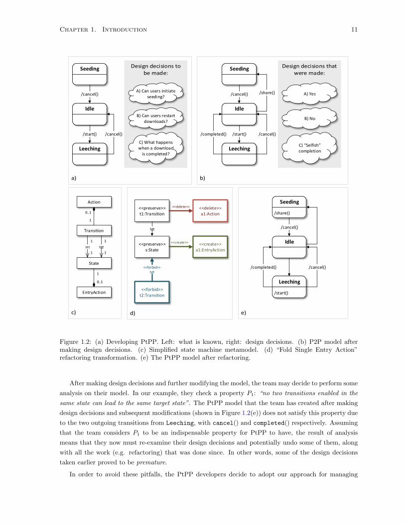
1.2 (a) Developing PtPP. Left: what is known, right: design decisions. (b) P2P model after
making design decisions. (c) Simplified state machine metamodel. (d) “Fold Single Entry
Action” refactoring transformation. (e) The PtPP model after refactoring. . . . . . . . . . 11
1.3 Partial model Mp2p used to articulate the uncertainty in Figure 1.2(a). Top: graphical
part of Mp2p. Bottom: propositional May formula for Mp2p. . . . . . . . . . . . . . . . . . 12
1.4 Semantics of the Mp2p partial model in Figure 1.3: six alternative designs of the PtPP
system. . . . . . . . . . . . . . . . . . . . . . . . . . . . . . . . . . . . . . . . . . . . . . . 14
1.5 (a-f) Versions of the concretizations in Figure 1.4 after being transformed using the FSEA
transformation in Figure 1.2(d). . . . . . . . . . . . . . . . . . . . . . . . . . . . . . . . . . 16
1.6 Partial model encoding the transformed concretizations shown in Figure 1.5. . . . . . . . 17
1.7 The elements that reify the “compromise” alternative solution to the decision point “what
happens when a download completes” are set to True and highlighted in green. Elements
reifying other alternative solutions are set to False and greyed out. Maybe elements that
are not part of this decision are left unaltered. . . . . . . . . . . . . . . . . . . . . . . . . . 18
2.1 Two example models, that are also concretizations of Mp2p, from Figure 1.2. . . . . . . . 21
2.2 Type graph and well-formedness constraints ΦSM of a simplified metamodel used for
defining State Machines. This type graph is a simplified version of the metamodel in
Figure 1.2(c). . . . . . . . . . . . . . . . . . . . . . . . . . . . . . . . . . . . . . . . . . . 21
2.3 Representing attributes using typed graphs: (a) Class shown in the concrete UML syntax.
(b) The same class shown as a typed graph. . . . . . . . . . . . . . . . . . . . . . . . . . . 22
2.4 (a) The graph union of the models in Figures 2.1(a,b). (b) An acyclic typed graph m1.
(c) An acyclic typed graph m2. (d) The graph union of m1 and m2 is not acyclic. . . . . . 24
2.5 (a, b) Simplified UML Class Diagram models ma and mb. (c) Model mc resulting from
the application of REV to mb. (d) Simplified UML Class Diagram metamodel. (e) Trans-
formation rule REV for doing the Encapsulate Variable refactoring. . . . . . . . . . . . . 26
2.6 Parts of the rule REV . Each rule part contains only those elements whose label appears
in bold serif font. . . . . . . . . . . . . . . . . . . . . . . . . . . . . . . . . . . . . . . . . 27
2.7 (a) Model C1. (b) Model C2, resulting from applying F1 to C1. (c) Model C3, resulting
from applying F2 to C1. (d) Model C4, resulting from applying F2 to C3. (e) Transfor-
mation rule F1. (f) Transformation rule F2. (g) Transformation rule F3. (h) Model C5,
resulting from applying F3 to C1. (i) Model C6, resulting from applying F3 to C1. . . . 28
xii

3.1 Example sketches produced by users when asked to model uncertainty in a modelling task. 34
3.2 (a) Simple Box metamodel B, (b) partialized Box metamodel Bp, (c) partial model, in-
stance of Bp, that violates the multiplicity constraints of B. . . . . . . . . . . . . . . . . . 36
3.3 (a) Base language in PtPP: simplified UML State Machine metamodel. (b) Partial State
Machine metamodel. (c) Fragment from Mp2p. (d) A different way to model the same
fragment that is expressible in the abstract syntax but not in the concrete syntax (May
formula not shown). . . . . . . . . . . . . . . . . . . . . . . . . . . . . . . . . . . . . . . . 37
3.4 Some equivalent partial models that encode the set S¬P2, consisting of the two con-
cretizations in Figures 1.4(c, d): (a) in GRF (b) in PRF (c) containing two superfluous
Maybe-annotated atoms (Bt and Ba). . . . . . . . . . . . . . . . . . . . . . . . . . . . . . . 41
3.5 An example product line, representing a family of vending machines. The product line
consists of a Feature Model (left) and a Featured Transition System (right). Elements
of the transition system are annotated with presence conditions. Image source: [Classen
et al., 2010]. . . . . . . . . . . . . . . . . . . . . . . . . . . . . . . . . . . . . . . . . . . . . 47
4.1 Checking properties with partial models (E1) compared to classically (E2). Speedup (E2E1 )
versus model size for different degrees of uncertainty. . . . . . . . . . . . . . . . . . . . . . 59
5.1 (a) partial model M1, showing points of uncertainty. (b) M1 as a typed graph (UML
abstract syntax). (c-e) Concretizations m11,m12,m13 of M1. . . . . . . . . . . . . . . . . 64
5.2 Transformation rule REV for doing the Encapsulate Variable refactoring. . . . . . . . . . 65
5.3 (a-c) Classical models resulting from applying REV to the classical models in Figure 5.1(c-
e). (d) The result of applying the lifted version REV to M1 directly: the partial model
M2. . . . . . . . . . . . . . . . . . . . . . . . . . . . . . . . . . . . . . . . . . . . . . . . . 65
5.4 Applying the lifted version of REV to the motivating example. Left: input model M1,
May graph and truth table of the May formula. Right: output model M2, May graph and
truth table of the May formula. . . . . . . . . . . . . . . . . . . . . . . . . . . . . . . . . 67
6.1 Construction of GRF based on Algorithm 3 (E4), compared to construction based on
Algorithm 1 (E3): speedup versus model size for different degrees of uncertainty. . . . . . 80
7.1 The Uncertainty Waterfall: an idealized timeline of uncertainty management. . . . . . . . 84
7.2 Degree of uncertainty in different stages of the Uncertainty Waterfall. . . . . . . . . . . . 84
7.3 The Extended Uncertainty Waterfall. . . . . . . . . . . . . . . . . . . . . . . . . . . . . . . 85
7.4 Uncertainty management operators overlayed on the Extended Uncertainty Waterfall. . . 92
7.5 Screenshot of Mu-Mmint. Left: interactive workspace showing different versions of PtPP.
Middle: Graphical partial model Mp2p for PtPP. Model elements that reify solutions in
the uncertainty tree are annotated with (M). Right: Decision tree for Mp2p. . . . . . . . . 96
7.6 Highlighting the elements that reify the “compromise” alternative solution in Mu-Mmint. 97
7.7 Highlighting alternatives for the decision “What happens when a download is completed?”
in Mu-Mmint. Maybe elements realizing the “benevolent” scenario are coloured in blue,
those realizing the “selfish” scenario – in green, and those realizing the “compromise”
scenario – in red. . . . . . . . . . . . . . . . . . . . . . . . . . . . . . . . . . . . . . . . . . 98
7.8 Visualizing a counterexample to property P2 in Mu-Mmint. . . . . . . . . . . . . . . . . 99
xiii
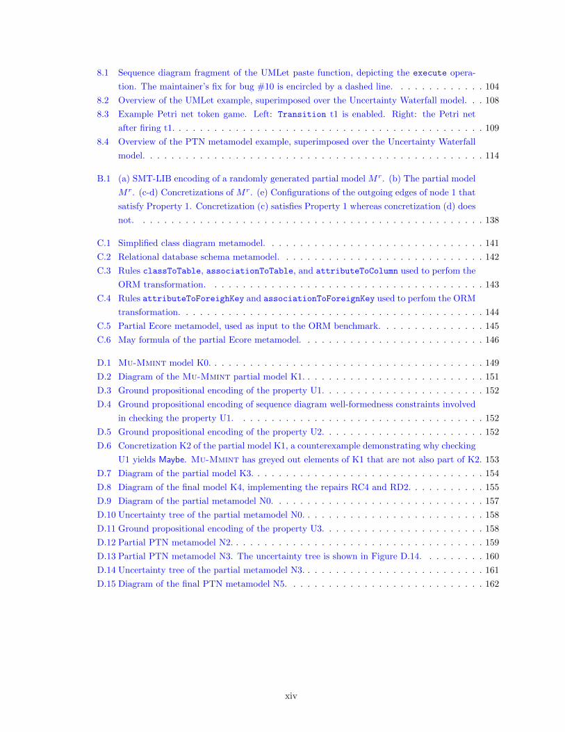
8.1 Sequence diagram fragment of the UMLet paste function, depicting the execute opera-
tion. The maintainer’s fix for bug #10 is encircled by a dashed line. . . . . . . . . . . . . 104
8.2 Overview of the UMLet example, superimposed over the Uncertainty Waterfall model. . . 108
8.3 Example Petri net token game. Left: Transition t1 is enabled. Right: the Petri net
after firing t1. . . . . . . . . . . . . . . . . . . . . . . . . . . . . . . . . . . . . . . . . . . . 109
8.4 Overview of the PTN metamodel example, superimposed over the Uncertainty Waterfall
model. . . . . . . . . . . . . . . . . . . . . . . . . . . . . . . . . . . . . . . . . . . . . . . . 114
B.1 (a) SMT-LIB encoding of a randomly generated partial model Mr. (b) The partial model
Mr. (c-d) Concretizations of Mr. (e) Configurations of the outgoing edges of node 1 that
satisfy Property 1. Concretization (c) satisfies Property 1 whereas concretization (d) does
not. . . . . . . . . . . . . . . . . . . . . . . . . . . . . . . . . . . . . . . . . . . . . . . . . 138
C.1 Simplified class diagram metamodel. . . . . . . . . . . . . . . . . . . . . . . . . . . . . . . 141
C.2 Relational database schema metamodel. . . . . . . . . . . . . . . . . . . . . . . . . . . . . 142
C.3 Rules classToTable, associationToTable, and attributeToColumn used to perfom the
ORM transformation. . . . . . . . . . . . . . . . . . . . . . . . . . . . . . . . . . . . . . . 143
C.4 Rules attributeToForeighKey and associationToForeignKey used to perfom the ORM
transformation. . . . . . . . . . . . . . . . . . . . . . . . . . . . . . . . . . . . . . . . . . . 144
C.5 Partial Ecore metamodel, used as input to the ORM benchmark. . . . . . . . . . . . . . . 145
C.6 May formula of the partial Ecore metamodel. . . . . . . . . . . . . . . . . . . . . . . . . . 146
D.1 Mu-Mmint model K0. . . . . . . . . . . . . . . . . . . . . . . . . . . . . . . . . . . . . . . 149
D.2 Diagram of the Mu-Mmint partial model K1. . . . . . . . . . . . . . . . . . . . . . . . . . 151
D.3 Ground propositional encoding of the property U1. . . . . . . . . . . . . . . . . . . . . . . 152
D.4 Ground propositional encoding of sequence diagram well-formedness constraints involved
in checking the property U1. . . . . . . . . . . . . . . . . . . . . . . . . . . . . . . . . . . 152
D.5 Ground propositional encoding of the property U2. . . . . . . . . . . . . . . . . . . . . . . 152
D.6 Concretization K2 of the partial model K1, a counterexample demonstrating why checking
U1 yields Maybe. Mu-Mmint has greyed out elements of K1 that are not also part of K2. 153
D.7 Diagram of the partial model K3. . . . . . . . . . . . . . . . . . . . . . . . . . . . . . . . . 154
D.8 Diagram of the final model K4, implementing the repairs RC4 and RD2. . . . . . . . . . . 155
D.9 Diagram of the partial metamodel N0. . . . . . . . . . . . . . . . . . . . . . . . . . . . . . 157
D.10 Uncertainty tree of the partial metamodel N0. . . . . . . . . . . . . . . . . . . . . . . . . . 158
D.11 Ground propositional encoding of the property U3. . . . . . . . . . . . . . . . . . . . . . . 158
D.12 Partial PTN metamodel N2. . . . . . . . . . . . . . . . . . . . . . . . . . . . . . . . . . . . 159
D.13 Partial PTN metamodel N3. The uncertainty tree is shown in Figure D.14. . . . . . . . . 160
D.14 Uncertainty tree of the partial metamodel N3. . . . . . . . . . . . . . . . . . . . . . . . . . 161
D.15 Diagram of the final PTN metamodel N5. . . . . . . . . . . . . . . . . . . . . . . . . . . . 162
xiv
List of Algorithms
1 GRF Conversion. . . . . . . . . . . . . . . . . . . . . . . . . . . . . . . . . . . . . . . . . . 42
2 PRF Conversion . . . . . . . . . . . . . . . . . . . . . . . . . . . . . . . . . . . . . . . . . . 43
3 Construction of a partial model from a set of concrete models. . . . . . . . . . . . . . . . . 44
4 Valuation-to-model conversion. . . . . . . . . . . . . . . . . . . . . . . . . . . . . . . . . . . 54
5 Computing all concretizations of a given model that satisfy a given property. . . . . . . . . 77
xv
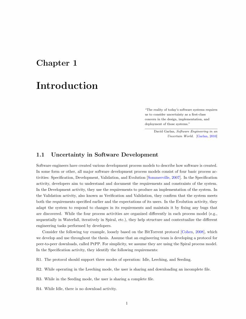
Chapter 1
Introduction
“The reality of today’s software systems requires
us to consider uncertainty as a first-class
concern in the design, implementation, and
deployment of those systems.”
David Garlan, Software Engineering in an
Uncertain World. [Garlan, 2010]
1.1 Uncertainty in Software Development
Software engineers have created various development process models to describe how software is created.
In some form or other, all major software development process models consist of four basic process ac-
tivities: Specification, Development, Validation, and Evolution [Sommerville, 2007]. In the Specification
activity, developers aim to understand and document the requirements and constraints of the system.
In the Development activity, they use the requirements to produce an implementation of the system. In
the Validation activity, also known as Verification and Validation, they confirm that the system meets
both the requirements specified earlier and the expectations of its users. In the Evolution activity, they
adapt the system to respond to changes in its requirements and maintain it by fixing any bugs that
are discovered. While the four process activities are organized differently in each process model (e.g.,
sequentially in Waterfall, iteratively in Spiral, etc.), they help structure and contextualize the different
engineering tasks performed by developers.
Consider the following toy example, loosely based on the BitTorrent protocol [Cohen, 2008], which
we develop and use throughout the thesis. Assume that an engineering team is developing a protocol for
peer-to-peer downloads, called PtPP. For simplicity, we assume they are using the Spiral process model.
In the Specification activity, they identify the following requirements:
R1. The protocol should support three modes of operation: Idle, Leeching, and Seeding.
R2. While operating in the Leeching mode, the user is sharing and downloading an incomplete file.
R3. While in the Seeding mode, the user is sharing a complete file.
R4. While Idle, there is no download activity.
1

Chapter 1. Introduction 2
Seeding
Idle
Leeching
/start()
Seeding
Idle
Leeching
/ cancel()
/start() /cancel()
(a) (b)
Figure 1.1: (a) Initial PtPP model, created in the Development activity. (b) The PtPP model aftergoing through the Evolution activity.
R5. While Idle, users can start a new download, thus switching to Leeching.
R6. It should always be possible to cancel sharing a file, returning to the Idle mode of operation.
In the Development activity, the team uses these requirements to architect an initial design of the pro-
tocol. This is shown in Figure 1.1(a), expressed as a state machine [Rumbaugh et al., 2004]. The
model uses a simplified version of the state machine modelling language, which is defined using a meta-
model [Atkinson and Kuhne, 2003], shown in Figure 1.2(c). Specifically, there is a state Idle, a state
Leeching (sharing and downloading an incomplete file), and a state Seeding (sharing a complete file).
When Leeching is initiated, the action start() is executed. In the Validation activity, the team checks
their implementation against the requirements. They discover that requirement R6 is not satisfied.
Therefore, in the following Evolution activity, they expand their design, producing the model shown in
Figure 1.1(b). In it, sharing from the states Seeding and Leeching can be cancelled, triggering the
action cancel().
While the different process activities correspond to different stages in the software lifecycle, they all
involve making decisions. In the PtPP example, in the Specification activity the team has to make deci-
sions such as: What happens when a download is completed? Should users be able to restart downloads?
In Development they have to decide issues such as: In what platform should PtPP be implemented?
Can the design be refactored to be more compact? In Verification they have to address decisions such
as: What are important properties that PtPP should satisfy? What verification method should be used?
And in Evolution, they must make decisions such as: Which requirements should be re-examined? Each
decision that the team makes shapes PtPP in specific ways, giving it some characteristics, capabilities or
behaviours, while restricting others. At any point in its lifecycle, a software system is the accumulated
result of answers to a myriad such questions about its every aspect.
In each development activity, developers may face a number of open decisions. However, they may
lack sufficient information to resolve them. For example:
• In the Development stage, the team might discover that some of the requirements were unclear [van
Lamsweerde, 2009]. For example, the combination of requirements R3 and R4 is unclear with re-
spect to which mode PtPP should be in when there is only uploading activity. The team must
therefore decide whether to refine the requirements or to allow uploading in the Idle state. How-

Chapter 1. Introduction 3
ever, setting up a new round of requirements elicitation with all the stakeholders may be non-trivial,
causing delays, during which the team does not have enough information to proceed.
• In the Evolution stage, the team may have multiple ways to fix an inconsistency bug [Nentwich
et al., 2003; Egyed et al., 2008]. For example, one strategy to make the PtPP model consistent with
the requirements is to make cancel() an action that is triggered when the added transitions are
made. Another strategy is to make cancel() an entry action of the Idle state. The latter solution
avoids duplication but depends on finalizing the requirements for Idle. This is an example where
delays on one “decision point” cascade to others.
• At any point during the development, the team might have to consolidate the views of multiple
stakeholders [Sabetzadeh and Easterbrook, 2006]. For example, assume that the organization
developing PtPP is structured so that the development team is different from the testing team. If
at any point in the development cycle the specifications used by the two teams are inconsistent
(e.g., between identifying the violation of requirement R6 and fixing it), the teams have to go
through a negotiation process to consolidate them in a single specification. Before that process is
completed, neither team has sufficient information about how PtPP should behave.
• The team may have to decide whether to provide a particular functionality as a runtime config-
uration option or whether it should be a point of variability [Chechik et al., 2016]. For example,
assume that the PtPP team is instead developing a product line [Pohl et al., 2005] of protocols
and are faced with the decision “Should the system allow users to restart downloads?” They can
decide to make it a runtime configuration option available to the users of every product or they
can opt to make it a feature [Kang et al., 1990] thus providing it by default for some products and
excluding it completely from the rest. However, making this decision requires further requirements
analysis and therefore it cannot be decided until the next iteration.
• An example of external factors impacting development is the decision about choosing an imple-
mentation platform for PtPP. This decision depends on non-technical parameters such as business
analysis, contractual obligations, licensing, marketing strategies, etc. Until that decision is made
by the organization developing PtPP, the development team cannot decide whether, for example,
to use particular optimization techniques, platform-specific design patterns, etc.
The uncertainty faced by developers who do not have sufficient information to make decisions about
their system is called design-time uncertainty [Ramirez et al., 2012]. Design-time uncertainty concerns
the content of a software system, and is different from uncertainty about the environment in which the
system is meant to operate (known as environmental uncertainty). In other words, it is uncertainty
that the developer has about what the system should be like, rather than about what conditions it
may face during its operation. For example, design-time uncertainty occurs if the team has insufficient
information to choose an implementation platform for PtPP. In contrast, environmental uncertainty
occurs if, for example, it is not possible to know whether there will be a network outage at the time
when a user decides to restart a download. To better illustrate the notion of design-time uncertainty,
we brainstormed various concerns that a developer faced with design-time uncertainty might have. The
resulting (incomplete) list contains several examples of such concerns and is shown in Table 1.1.
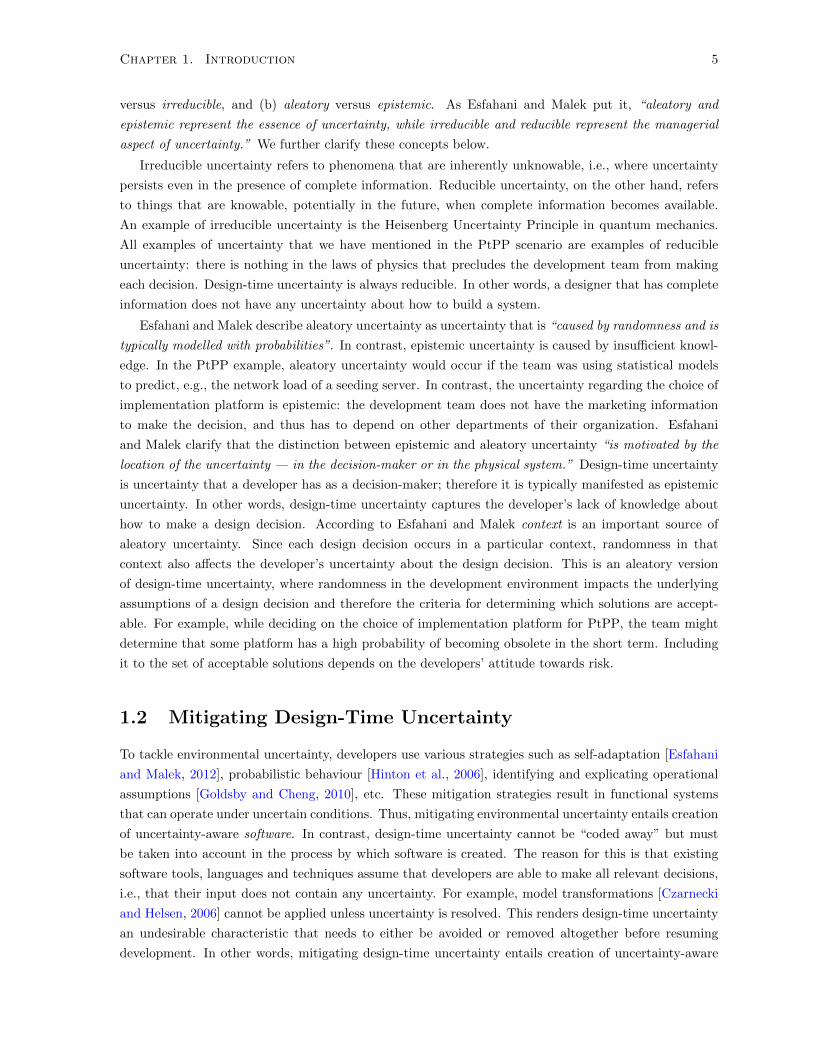
To further clarify the notion of design-time uncertainty, we refer to the philosophical classification
provided by [Esfahani and Malek, 2012], which describes uncertainty in terms of two axes: (a) reducible

Chapter 1. Introduction 4
Table 1.1: Examples of concerns a developer might have when faced with design-time uncertainty.# Concern1 What are the open decisions about the design of the system at this time?2 What criteria are relevant for making each decision?3 How likely is it that the criteria for making decisions will change?4 What are the candidate solutions for each open design decision?5 What criteria are relevant for a design to be considered a candidate solution?6 Is it possible to generate candidate solutions automatically?7 Which candidate solutions have been automatically generated and which where created by hand?8 How likely is it that the criteria for generating candidate solutions will change?9 How is each candidate solution expressed in the system?
10 Which parts of the system are affected by open design decisions?11 How are design decisions decomposed?12 Which design decisions do I intend to further decompose?13 What are dependencies between design decisions?14 What are the dependencies between candidate solutions?15 Have I described all dependencies between design decisions or between candidate solutions?16 Given a design decision, is its set of candidate solutions complete?17 Which design decisions am I still working on?18 What are relevant metadata about candidate solutions? (E.g., pros and cons)19 What are the trade-offs involved in making each design decision?20 What are relevant metadata about design decisions? (E.g., importance, priority)21 What is it that causes me to not be able to make a design decision?22 What is the rationale for each design decision?23 What is the rationale for each candidate solution?24 What is the rationale for the way each candidate solution is expressed in the system?25 Is the expression of each candidate solution in the system stable?26 What are commonalities and differences between candidate solutions?27 What parts of a given candidate solution am I still working on?28 What properties should all candidate solutions satisfy?29 What properties should be satisfiable by at least one candidate solution?30 Which candidate solutions can be incorporated into the system using conditionals?31 Which candidate solutions can become configuration options?32 Which design decisions can become points of variability or adaptation?33 Which parts of the system are intentionally underspecified?34 Are the candidate solutions consistent/well-formed?35 Are they at the right level of abstraction?36 Who identified each design decision?37 Who proposed each candidate solution?38 Who can help me resolve a given design decision?39 Who is responsible for making each design decision?40 What are the design decisions that have been made about the system in the past?41 What was the rationale for making them?42 Who made them?43 Which past design decisions are affected by open design decisions?44 How are open design decisions affected by past decisions?45 Are there candidate solutions that were discarded in the past that might help in the present?46 Which design decisions were made provisionally in the past?47 What engineering tasks can be done at the part of the system that is affected by uncertainty?48 What engineering tasks can be done at the rest of the system?
Chapter 1. Introduction 5
versus irreducible, and (b) aleatory versus epistemic. As Esfahani and Malek put it, “aleatory and
epistemic represent the essence of uncertainty, while irreducible and reducible represent the managerial
aspect of uncertainty.” We further clarify these concepts below.
Irreducible uncertainty refers to phenomena that are inherently unknowable, i.e., where uncertainty
persists even in the presence of complete information. Reducible uncertainty, on the other hand, refers
to things that are knowable, potentially in the future, when complete information becomes available.
An example of irreducible uncertainty is the Heisenberg Uncertainty Principle in quantum mechanics.
All examples of uncertainty that we have mentioned in the PtPP scenario are examples of reducible
uncertainty: there is nothing in the laws of physics that precludes the development team from making
each decision. Design-time uncertainty is always reducible. In other words, a designer that has complete
information does not have any uncertainty about how to build a system.
Esfahani and Malek describe aleatory uncertainty as uncertainty that is “caused by randomness and is
typically modelled with probabilities”. In contrast, epistemic uncertainty is caused by insufficient knowl-
edge. In the PtPP example, aleatory uncertainty would occur if the team was using statistical models
to predict, e.g., the network load of a seeding server. In contrast, the uncertainty regarding the choice of
implementation platform is epistemic: the development team does not have the marketing information
to make the decision, and thus has to depend on other departments of their organization. Esfahani
and Malek clarify that the distinction between epistemic and aleatory uncertainty “is motivated by the
location of the uncertainty — in the decision-maker or in the physical system.” Design-time uncertainty
is uncertainty that a developer has as a decision-maker; therefore it is typically manifested as epistemic
uncertainty. In other words, design-time uncertainty captures the developer’s lack of knowledge about
how to make a design decision. According to Esfahani and Malek context is an important source of
aleatory uncertainty. Since each design decision occurs in a particular context, randomness in that
context also affects the developer’s uncertainty about the design decision. This is an aleatory version
of design-time uncertainty, where randomness in the development environment impacts the underlying
assumptions of a design decision and therefore the criteria for determining which solutions are accept-
able. For example, while deciding on the choice of implementation platform for PtPP, the team might
determine that some platform has a high probability of becoming obsolete in the short term. Including
it to the set of acceptable solutions depends on the developers’ attitude towards risk.
1.2 Mitigating Design-Time Uncertainty
To tackle environmental uncertainty, developers use various strategies such as self-adaptation [Esfahani
and Malek, 2012], probabilistic behaviour [Hinton et al., 2006], identifying and explicating operational
assumptions [Goldsby and Cheng, 2010], etc. These mitigation strategies result in functional systems
that can operate under uncertain conditions. Thus, mitigating environmental uncertainty entails creation
of uncertainty-aware software. In contrast, design-time uncertainty cannot be “coded away” but must
be taken into account in the process by which software is created. The reason for this is that existing
software tools, languages and techniques assume that developers are able to make all relevant decisions,
i.e., that their input does not contain any uncertainty. For example, model transformations [Czarnecki
and Helsen, 2006] cannot be applied unless uncertainty is resolved. This renders design-time uncertainty
an undesirable characteristic that needs to either be avoided or removed altogether before resuming
development. In other words, mitigating design-time uncertainty entails creation of uncertainty-aware

Chapter 1. Introduction 6
software development methodologies.
Aleatory aspects of design-time uncertainty can be mitigated by techniques such as risk manage-
ment [Islam and Houmb, 2010; Boehm, 1991] and software estimation [Jones, 1998]. However, in the
face of epistemic design-time uncertainty, developers are forced to either:
(a) avoid working on the uncertain parts of the system, delaying the decisions as long as necessary,
(b) entirely remove uncertainty by making educated guesses based on experience so that work can
continue, or
(c) fork and maintain sets of alternative solutions.
We discuss these options below.
There is a considerable body of engineering research that focuses on avoiding design-time uncertainty
by delaying making decisions until the most opportune moment. This is an established practice in many
engineering disciplines, such as in industrial and mechanical engineering. A well known example is
the Toyota Production System (TPS) [Monden, 2011], which was developed in Japan during the mid-
20th century with the aim to eliminate inefficiencies in the production of automotive vehicles. The
TPS was a precursor to the practice of lean manufacturing, which in the software world inspired Lean
Software Engineering [Poppendieck and Poppendieck, 2003a; Ladas, 2009], one of the tenets of the Agile
methodology [Fowler and Highsmith, 2001; Martin, 2003]. While Agile is becoming increasingly popular,
it is not (to use the phrase coined by Fred Brooks [Brooks, 1995]) a “silver bullet” that is appropriate in
every organizational setting and project. This is evidenced by the proliferation of literature discussing
success factors [Misra et al., 2009; Ramesh et al., 2006] and challenges to its adoption [Nerur et al., 2005].
Moreover, while the stated goal of lean methods is to eliminate waste, i.e., under-utilization of resources,
that is not necessarily the case in practice. For example, Ikonen et al. conducted a seven-week empirical
study to identify sources of waste in lean development [Ikonen et al., 2010], focusing specifically on the
Kanban method [Ladas, 2009]. Among other sources of waste, they identified that there were delays due
to some developers waiting, e.g., for the completion of tasks that were under-estimated, for clarification
of requirements, or for customer validation. Thus, delaying decisions is not always the most effective
way to handle design-time uncertainty.
In practice, developers often rely on experience and craftsmanship to make and keep track of provi-
sional decisions that artificially remove uncertainty from their artifacts so that development can continue.
This increases the risk of having to backtrack their work if new information shows that the provisional
decisions were wrong. Even worse, it can mean committing too early to design decisions that cannot
be reversed without significant costs, when it would be more desirable to keep many alternative options
open for consideration. In fact, the skillful management of such provisionality is a defining characteristic
of expert software designers [Petre, 2009]. Agile proposes to manage these risks by employing short iter-
ation cycles and frequent customer feedback. As discussed earlier, Agile is not a “silver bullet”, so such
practices are not always feasible. Additionally, there is the problem of keeping track of which decisions
were made provisionally and which were not. This is aggravated by the preference in Agile for “working
software over comprehensive documentation” [Fowler and Highsmith, 2001]. Unless explicit traceability
and provenance is maintained, the provisional character of a decision may be forgotten, thus implicitly
turning the decision into a premature, undocumented commitment.
Given a design decision, engineers might choose to consider all alternative solutions, therefore forking
the project into parallel streams. This allows them to keep their options open, as well as to potentially

Chapter 1. Introduction 7
turn decisions into variability points, thus creating families of products that meet the needs of more
than one customer [Pohl et al., 2005; Chechik et al., 2016]. Forking can be done in a vigorous and
systematic way. For example, the “Programming by Optimization” (PbO) approach, developed by
Holger Hoos [Hoos, 2012], aims to help software developers avoid premature optimization commitments in
settings where multiple algorithms can accomplish the same computational task, albeit in different ways.
Design decisions and alternatives are explicitly tracked until the time when designers have enough hard
evidence (obtained systematically using machine learning) regarding the optimality of each algorithm to
make informed decisions. However, forking does not scale as a generic solution to mitigating design-time
uncertainty due to the combinatoric explosion of possibilities in the case where multiple decision points
must be managed. Additionally, since every fork must be maintained separately, every forking approach
is limited by the size of the set of possible solutions to a decision point. Without any structure to
describe their commonalities and differences, it is impossible to reuse results across forks. Thus, every
engineering task such as verification, transformation, evolution, etc. has to be repeated for each fork,
which is expensive and error-prone.
Thesis Statement. In this thesis, we introduce a novel methodological approach for managing epis-
temic design-time uncertainty, that combines ideas from the aforementioned mitigation strategies. Specif-
ically, we show that it is possible to defer design decisions while efficiently maintaining and working with
the encoding of the set of possible designs they entail. Once enough information is available, decisions
can be made by systematically reducing this set. Similar to techniques that delay decision making,
our approach aims to help developers avoid premature decisions. However, instead of routing around
the parts of the system that are uncertain, we expand them to the set of possible solutions. Unlike
forking approaches, however, we use a special-purpose formalism, called “partial models”, to encode the
set of solutions in a compact and exact manner. Partial models are first class development artifacts that
can be used to perform engineering tasks. This allows engineering work to proceed but, in contrast to
approaches that employ provisionality, no decision is made prematurely. Once enough information is ac-
quired, it is systematically incorporated in partial models through a process of formal refinement. These
characteristics of partial models allow us to create a methodology specifically for managing design-time
uncertainty.
In the rest of the thesis, we often refer to epistemic design-time uncertainty as “design-time uncer-
tainty” or simply as “uncertainty”, provided that the context is unambiguous.
1.3 Scope of Design-Time Uncertainty Management
The two core ideas of the approach presented in this thesis are the deferral of design decisions and
the use of formal artifacts to explicitly capture what is and is not known. This combination is not
new: it has been studied extensively in the field of behavioural specification [Larsen and Thomsen,
1988]. The novelty of our approach lies in expanding that work for arbitrary modelling languages,
not just partial behavioural models with carefully defined semantics. In this section, we use concepts
from epistemology and partial behavioural modelling to precisely define the scope of our approach for
design-time uncertainty management.
The idea of creating formal artifacts that incorporate the developer’s lack of knowledge about some
part of a software system is not new. By definition, formal specification languages are used to explicate

Chapter 1. Introduction 8
what is known about a system. The unknown is therefore often modelled indirectly, by omission.
Specifically: when specifying a system, scope1 defines what elements are relevant to the system, and span
– what level of abstraction is acceptable. In the PtPP example, concerns such as logging and digital
rights management are outside the scope of the model. Implementation details such as establishing
TCP/IP connections are outside its span.
In this thesis, we make an assumption that the scope and span are known to the developers. In other
words, we do not discuss the process of identifying which parts of their system they are uncertain about
and what the decision points are.
A common convention in behavioural modelling is that elements that are outside the scope and
span of the specification are ones about which the developer does not care. A different interpretation
is that such elements represent “unknown unknowns”, a term we borrow from the simple epistemology
of ignorance famously defined by the former US Secretary of Defence, Donald Rumsfeld prior to the
2003 invasion of Iraq, during a Press Conference at the NATO Headquarters, in Brussels on June 6,
2002 [Rumsfeld, 2011]:
“[As] we know, there are known knowns; there are things we know we know. We also know
there are known unknowns; that is to say we know there are some things we do not know.
But there are also unknown unknowns the ones we don’t know we don’t know.2”
Design-time uncertainty encompasses both “known unknowns” and “unknown unknowns”. Elements
outside the scope and span of a specification (“unknown unknowns”) are those that result from decisions
that have an unknown set of possible solutions. “Known unknowns” result from decisions that have a
known set of possible answers.
For example, we assume that the team developing PtPP is uncertain about three decisions, listed
on the right of Figure 1.2(a): (D1) Can users initiate seeding? (D2) Can downloads be restarted?
(D3) what policy is followed when leeching ends? The first two questions are closed: they have a “yes”
or “no” answer, and are thus “known unknowns”. The third question is open, as it does not imply a set
of acceptable candidate policies. It is therefore an “unknown unknown”.
In the context of software development, the relationship between “unknown unknowns” and “known
unknowns” can be understood as a process of elicitation. A design decision is first posed as an open
question, the set of its possible solutions being unknown. As the engineers engage and work through
the problem, a set of possible solutions emerges. The design decision thus becomes a closed question:
“which of the possible solutions should be selected?” In our example, as the PtPP team starts working on
decision (D3), they decide that there are three possible alternatives regarding the policy about completed
downloads: (a) the “benevolent” option which automatically starts Seeding, (b) the “selfish” option
described earlier, and (c) a “compromise” option where no new connections are accepted while waiting
for existing peers to complete their copies. The decision therefore becomes a choice between these three
candidate solutions.
In this thesis, we scope our treatment of design-time uncertainty to “known unknowns”. Specifically,
we do not investigate the process by which a development team elicits candidate solutions for an open
question. Instead, we assume that this process has already taken place and that for each design decision
1In this section, the word “scope” is used both to refer to the scope of the approach presented in the thesis, as well asto the scope of a software specification. The meaning of the word is the same for both usages.
2The philosopher Slavoj Zizek has noted that Rumsfeld’s epistemology is incomplete, since it does not include “unknownknowns”, i.e., unstated assumptions [Zizek, 2006].
Chapter 1. Introduction 9
we are given a finite set of possible solutions. We also assume that the development team has concluded
how to implement each candidate solution. Partial models are then used to compactly and exactly encode
the set of candidate solutions.
Given that for each design decision the set of candidate solutions is assumed to be known, a devel-
opment team may decide to include all or some solutions to the software system, allowing any of them
to be used as required. This can be done, for example, by making the design decision a conditional
choice in code or a configuration option, or by making it a point of variability [Pohl et al., 2005] or
runtime adaptation [Bencomo et al., 2008]. We consider this to be a particular way to resolve uncer-
tainty, that effectively turns “known unknowns” into “known knowns”. In other words, in such cases
uncertainty about the design is considered resolved, even if the system is allowed to change in response
to environmental uncertainty or user preferences. In this thesis, we do not address the process required
to implement such resolutions of design-time uncertainty.
A conventional way to reason about “known unknowns” is the closed-world assumption [Shepherdson,
1984] via the use of underspecification. Specifically, elements that are within the given scope and span,
but are not present in the specification are underspecified. In practice, this is often used to indicate that
these elements are to be re-visited at a later point when more information becomes available. Thus,
an underspecified system represents a set of fully specified possibilities. Nondeterminism is a common
way to interpret underspecification in the context of behavioural modelling. Underspecification is used
to implicitly (through omission) hint at what developers are uncertain about. However, the aim of our
approach is to support decision deferral while allowing developers to perform engineering tasks with the
artifacts containing design-time uncertainty. Performing engineering tasks with such artifacts requires
design-time uncertainty to be explicitly modelled; otherwise, it cannot be manipulated or reasoned with.
Therefore, the strategy of modelling design-time uncertainty through underspecification is not suitable
for our purposes.
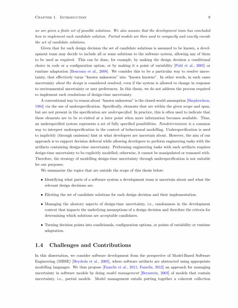
We summarize the topics that are outside the scope of this thesis below:
• Identifying what parts of a software system a development team is uncertain about and what the
relevant design decisions are.
• Eliciting the set of candidate solutions for each design decision and their implementation.
• Managing the aleatory aspects of design-time uncertainty, i.e., randomness in the development
context that impacts the underlying assumptions of a design decision and therefore the criteria for
determining which solutions are acceptable candidates.
• Turning decision points into conditionals, configuration options, or points of variability or runtime
adaptation.
1.4 Challenges and Contributions
In this dissertation, we consider software development from the perspective of Model-Based Software
Engineering (MBSE) [Beydeda et al., 2005], where software artifacts are abstracted using appropriate
modelling languages. We thus propose [Famelis et al., 2011; Famelis, 2012] an approach for managing
uncertainty in software models by doing model management [Bernstein, 2003] of models that contain
uncertainty, i.e., partial models. Model management entails putting together a coherent collection

Chapter 1. Introduction 10
of operators that allow performing different model manipulation tasks. Our approach to uncertainty
management is thus outlined in Chapter 7 as a coherent collection of software engineering tasks that can
be accomplished using partial models. Specifically, we consider partial models to be first-class artifacts
that allow developers to:
(a) articulate their uncertainty,
(b) defer its resolution, while continuing development with tasks such as:
(i) performing automated verification and diagnosis, as well as
(ii) applying model transformations, and finally
(c) systematically resolve uncertainty by incorporating new information.
To illustrate the meaning of each of the verification and transformation tasks, we first show how they
can be applied to the PtPP example, without the use of partial models. We then use the PtPP example
to describe the main challenges and the contributions of the thesis.
For each area of contribution, we also indicate which concerns from Table 1.1 the approach helps
address. Concerns from Table 1.1 that are not referenced in this section, are outside the scope of the
thesis, as discussed in the previous sections.
Illustration of the PtPP scenario. In our scenario, the PtPP developers encountered uncertainty
regarding three decisions, listed on the right of Figure 1.2(a). Specifically, the team is uncertain about
the following decisions: (D1) Can users initiate seeding? (D2) Can downloads be restarted? (D3) what
policy is followed when leeching ends? The team further elicited three possible solutions to (D3): (a) a
“benevolent” option which automatically starts Seeding, (b) a “selfish” option described earlier, and
(c) a “compromise” option where no new connections are accepted while waiting for existing peers to
complete their copies.
Assume that the development team decides that their preferred strategy for managing uncertainty
is to make provisional decisions. In our scenario, the team makes provisional choices for the three
design decisions, as shown in Figure 1.2(b). Specifically: 1. Users can initiate seeding (indicated by the
transition with action share()). 2. Downloads are not restarted (no effect on the model). 3. The “selfish”
policy is adopted: at the end of Leeching, PtPP goes directly to Idle, not letting other connected peers
to complete their work (indicated by the transition with action completed()). .
In the course of developing PtPP, the team may do additional work on the model. Refactoring is
a common task done during development. For example, the team could refactor PtPP with a transfor-
mation such as the rewriting rule “Fold Single Entry Action” (FSEA) shown in Figure 1.2(d). FSEA is
expressed as a graph rewriting transformation rule [Ehrig et al., 2006] using the notation of the Henshin
model transformation engine [Arendt et al., 2010]. The rule tries to match a State s that has only one
incoming Transition t1. The “negative application condition” (indicated by << forbid >>) stops the
refactoring from being applied if there exists a second incoming Transition t2. Otherwise, it deletes
Action a1 of t1 (indicated by << delete >>) and adds a new EntryAction with the same name (in-
dicated by << create >>), associating it with s. The result of refactoring PtPP with FSEA is shown
in Figure 1.2(e), where the actions share() and start() have been respectively folded into the states
Seeding and Leeching.
Chapter 1. Introduction 11
A) Can users initiate seeding?
B) Can users restart downloads?
C) What happens when a download
is completed?
Seeding
Idle
Leeching
/cancel()
/start() /cancel()
A) Yes
B) No
C) Selfish completion
Seeding
Idle
Leeching
/cancel()
/start() /cancel()
/share()
/completed()
Transition
Action
0..1
1
State
1
1
src
1
1
tgt
EntryAction
0..1
1
<<preserve>>t1:Transition
<<delete>>a1:Action
<<preserve>>s:State
<<forbid>>t2:Transition
<<create>>a1:EntryAction
<<forbid>>tgt
tgt
<<delete>>
<<create>>
Seeding
/share()
Idle
Leeching
/start()
/cancel()
/cancel()/completed()
Figure 1.2: (a) Developing PtPP. Left: what is known, right: design decisions. (b) P2P model aftermaking design decisions. (c) Simplified state machine metamodel. (d) “Fold Single Entry Action”refactoring transformation. (e) The PtPP model after refactoring.
After making design decisions and further modifying the model, the team may decide to perform some
analysis on their model. In our example, they check a property P1: “no two transitions enabled in the
same state can lead to the same target state”. The PtPP model that the team has created after making
design decisions and subsequent modifications (shown in Figure 1.2(e)) does not satisfy this property due
to the two outgoing transitions from Leeching, with cancel() and completed() respectively. Assuming
that the team considers P1 to be an indispensable property for PtPP to have, the result of analysis
means that they now must re-examine their design decisions and potentially undo some of them, along
with all the work (e.g. refactoring) that was done since. In other words, some of the design decisions
taken earlier proved to be premature.
In order to avoid these pitfalls, the PtPP developers decide to adopt our approach for managing

Chapter 1. Introduction 12
Seeding
Idle Leeching
/cancel()
/start()
/cancel()
/completed()
/share()
/restart()
/completed()
/completed()/peersDone()
Finishing
BtCt
Dt
EtFs
Gt
Aa Ba
Ca
Da
EaGa
At
((¬At ∧ Bt ∧ ¬Dt ∧ ¬Et ∧ ¬Fs)∨(At ∧ ¬Bt ∧ Dt ∧ ¬Et ∧ ¬Fs)∨(At ∧ ¬Bt ∧ ¬Dt ∧ Et ∧ Fs) )∧
(At⇔ Aa) ∧ (Bt⇔ Ba) ∧ (Ct⇔ Ca) ∧ (Dt⇔ Da)∧(Fs⇔ Et⇔ EaGt⇔ Ga)
Figure 1.3: Partial model Mp2p used to articulate the uncertainty in Figure 1.2(a). Top: graphical partof Mp2p. Bottom: propositional May formula for Mp2p.
design time uncertainty. In the following, we illustrate the main challenges in supporting the PtPP team
defer design decisions while still developing the protocol and the contributions made in this thesis to
address them.
1.4.1 Articulating uncertainty
Challenges The main challenge is to create appropriate abstractions and representations to enable
the efficient representation of uncertainty by developers in machine-processable software artifacts. There
are thus two major sub-problems: (a) creating a user-friendly notation for expressing uncertainty, and
(b) equipping the notation with formal semantics, so that automated techniques can be applied.
As discussed in Section 1.3, we assume that for each design decision, developers have elicited a finite
set of candidate solutions. Thus, an additional challenge is to create an effective process for expressing
the set as a partial model.
Contributions We address the first two challenges by using the approach illustrated below and dis-
cussed in detail in Chapter 3. With respect to the third challenge, we provide an algorithm for automat-
ically constructing a partial model from the given set of solutions in Section 3.4. Additionally, the tool
Mu-Mmint, presented in Chapter 7, provides an interactive editor for creating partial models. However,

Chapter 1. Introduction 13
since the tool is a proof-of-concept prototype, we do not attempt to study the effectiveness and usability
of its editor as the main method for the creation of partial models.
At the start of the PtPP scenario, the team’s design may be separated into known and unknown
parts, as shown in Figure 1.2(a). In our approach, this information is captured in a single partial model
Mp2p, shown in Figure 1.3.
The top part of Figure 1.3 shows the graphical part of Mp2p. It consists of a model expressed in the
same concrete syntax as the original PtPP model fragment, with the addition of annotations (represented
as seven-pointed star icons) to some elements. These are called Maybe elements and are used to explicate
points of uncertainty in the model. We use propositional variables as aliases for individual Maybe element
decisions. For example, the transition share() between Idle and Seeding has two seven-pointed star
icons annotations, with the variables At and Aa for the transition and its action respectively. These
indicate that the developer is unsure whether to include them in the model. For example, setting Aa to
True means that she decides to include the action share(), False to exclude it.
The bottom part of Figure 1.3 shows the propositional May formula of Mp2p. This formula is used
to explicate dependencies between points of uncertainty. For example, it specifies that each transition
co-occurs with its corresponding action. Additionally, it specifies what are allowable configurations
of Maybe elements if uncertainty is resolved. According to the solutions elicited by the team, the May
formula allows three possible solutions to the policy about completed downloads: “benevolent”, “selfish”,
and “compromise”. As shown in Figure 1.2(a), a different point of uncertainty is whether users should
be able to initiate seeding (i.e., having a transition share from Idle). The May formula in Figure 1.3,
expresses the team’s decision to correlate the two points of uncertainty, by allowing the ability to start
seeding only for the “selfish” and the “compromise” behavioural scenarios.
The model Mp2p compactly encodes the set of models representing all possible ways to resolve uncer-
tainty. Each such model is called a concretization. For illustration purposes, we show the complete set of
concretizations of the Mp2p partial model in Figure 1.4(a-f). For example, the model in Figure 1.2(b) is
the same as the concretization shown in Figure 1.4(c). Moreover, the models in Figure 1.4(a,c,e) imple-
ment the “benevolent”, “selfish” and “compromise” designs, respectively. The models in Figure 1.4(b,d,f)
augment the previous ones with restarts.
This approach helps address concerns 1, 4, 9, 10, 11, 13, 14, 26, and 35 from Table 1.1, by allowing
developers to express their uncertainty within the model of the software system, as well as the different
dependencies between the different concretizations.
1.4.2 Performing automated verification
Challenges Our first task is to identify the kinds of properties that can be verified in the presence
of uncertainty. Subsequently, we need to develop appropriate verification techniques to efficiently check
such properties. We also must determine what useful feedback we can provide to developers.
Contributions We address these challenges by using the approach illustrated below and detailed in
Chapter 4. Using partial models, we can check syntactic properties, such as the property P1 in the PtPP
example (“no two transitions enabled in the same state can lead to the same target state”). The objective
of such checking is to determine whether a property Φ holds for all, some, or none of the partial model’s
concretizations. The result is therefore not boolean; instead, it can be either True (“the property holds
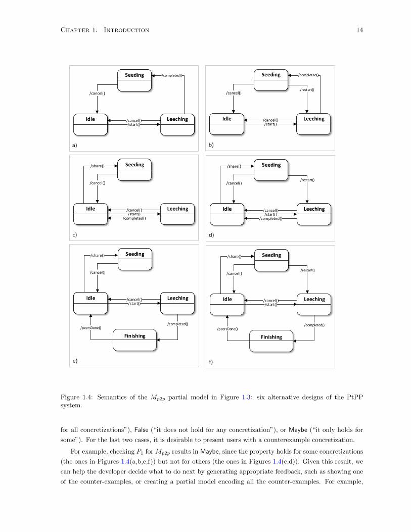
Chapter 1. Introduction 14
Seeding
Idle Leeching
/cancel()
/start()/cancel()
/completed() Seeding
Idle Leeching
/cancel()
/start()/cancel()
/restart()
/completed()
Seeding
Idle Leeching
/cancel()
/start()/cancel()
/share()
/completed()/peersDone()
Finishing
Seeding
Idle Leeching
/cancel()
/start()/cancel()
/share()
/restart()
/completed()/peersDone()
Finishing
Seeding
Idle Leeching
/cancel()
/start()/cancel()
/completed()
/share() Seeding
Idle Leeching
/cancel()
/start()/cancel()
/completed()
/share()
/restart()
Figure 1.4: Semantics of the Mp2p partial model in Figure 1.3: six alternative designs of the PtPPsystem.
for all concretizations”), False (“it does not hold for any concretization”), or Maybe (“it only holds for
some”). For the last two cases, it is desirable to present users with a counterexample concretization.
For example, checking P1 for Mp2p results in Maybe, since the property holds for some concretizations
(the ones in Figures 1.4(a,b,e,f)) but not for others (the ones in Figures 1.4(c,d)). Given this result, we
can help the developer decide what to do next by generating appropriate feedback, such as showing one
of the counter-examples, or creating a partial model encoding all the counter-examples. For example,
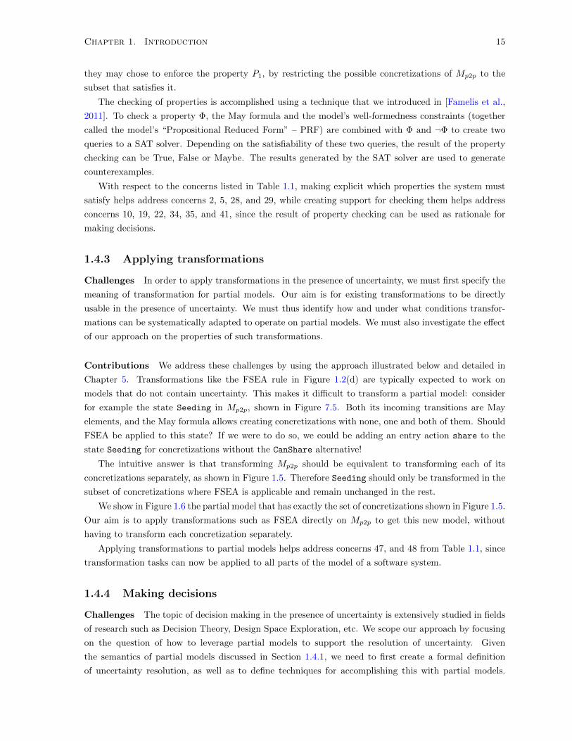
Chapter 1. Introduction 15
they may chose to enforce the property P1, by restricting the possible concretizations of Mp2p to the
subset that satisfies it.
The checking of properties is accomplished using a technique that we introduced in [Famelis et al.,
2011]. To check a property Φ, the May formula and the model’s well-formedness constraints (together
called the model’s “Propositional Reduced Form” – PRF) are combined with Φ and ¬Φ to create two
queries to a SAT solver. Depending on the satisfiability of these two queries, the result of the property
checking can be True, False or Maybe. The results generated by the SAT solver are used to generate
counterexamples.
With respect to the concerns listed in Table 1.1, making explicit which properties the system must
satisfy helps address concerns 2, 5, 28, and 29, while creating support for checking them helps address
concerns 10, 19, 22, 34, 35, and 41, since the result of property checking can be used as rationale for
making decisions.
1.4.3 Applying transformations
Challenges In order to apply transformations in the presence of uncertainty, we must first specify the
meaning of transformation for partial models. Our aim is for existing transformations to be directly
usable in the presence of uncertainty. We must thus identify how and under what conditions transfor-
mations can be systematically adapted to operate on partial models. We must also investigate the effect
of our approach on the properties of such transformations.
Contributions We address these challenges by using the approach illustrated below and detailed in
Chapter 5. Transformations like the FSEA rule in Figure 1.2(d) are typically expected to work on
models that do not contain uncertainty. This makes it difficult to transform a partial model: consider
for example the state Seeding in Mp2p, shown in Figure 7.5. Both its incoming transitions are May
elements, and the May formula allows creating concretizations with none, one and both of them. Should
FSEA be applied to this state? If we were to do so, we could be adding an entry action share to the
state Seeding for concretizations without the CanShare alternative!
The intuitive answer is that transforming Mp2p should be equivalent to transforming each of its
concretizations separately, as shown in Figure 1.5. Therefore Seeding should only be transformed in the
subset of concretizations where FSEA is applicable and remain unchanged in the rest.
We show in Figure 1.6 the partial model that has exactly the set of concretizations shown in Figure 1.5.
Our aim is to apply transformations such as FSEA directly on Mp2p to get this new model, without
having to transform each concretization separately.
Applying transformations to partial models helps address concerns 47, and 48 from Table 1.1, since
transformation tasks can now be applied to all parts of the model of a software system.
1.4.4 Making decisions
Challenges The topic of decision making in the presence of uncertainty is extensively studied in fields
of research such as Decision Theory, Design Space Exploration, etc. We scope our approach by focusing
on the question of how to leverage partial models to support the resolution of uncertainty. Given
the semantics of partial models discussed in Section 1.4.1, we need to first create a formal definition
of uncertainty resolution, as well as to define techniques for accomplishing this with partial models.

Chapter 1. Introduction 16
Seeding
/completed()
Idle Leeching
/start()
/cancel()
/cancel()
Seeding
/completed()
Idle Leeching
/cancel()
/start()/cancel()
/restart()
Seeding
/share()
Idle Leeching
/start()
/cancel()
/cancel()
/peersDone()
Finishing
Seeding
/share()
Idle Leeching
/cancel()
/start()/cancel()
/restart()
/peersDone()
Finishing
Seeding
/share()
Idle Leeching
/start()
/cancel()
/cancel()
/completed()
Seeding
/share()
Idle Leeching
/cancel()
/start()/cancel()
/completed()
/restart()
/completed() /completed()
Figure 1.5: (a-f) Versions of the concretizations in Figure 1.4 after being transformed using the FSEAtransformation in Figure 1.2(d).
Subsequently, we must address the issue of the effect of uncertainty resolution to the properties of
partial models. Finally, we need to provide a mechanism for tracing the design decisions across the
lifecycle of software artifacts.
Contributions We address these challenges by using the refinement approach presented in Chapter 6.
Specifically, supporting decision deferral means allowing developers to make decisions in a systematic
way when the time is right. This can be done either by enforcing properties such as those discussed in
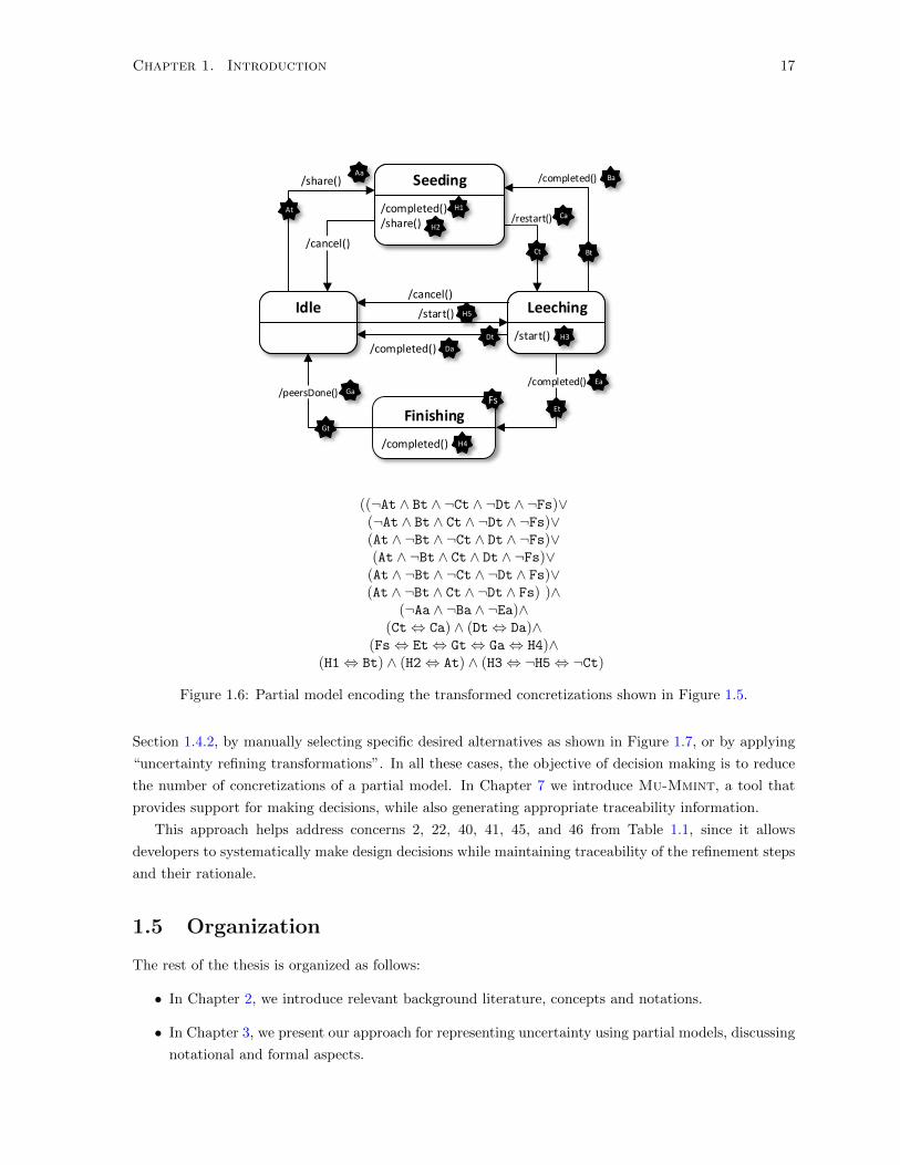
Chapter 1. Introduction 17
Seeding
/completed()/share()
Idle Leeching
/start()
/cancel()
/start()
/cancel()
/completed()
/share()
/restart()
/completed()
/completed()/peersDone()
Finishing
BtCt
Dt
EtFs
Gt
AaBa
Ca
Da
EaGa
At
/completed()
H1
H2
H3
H4
H5
((¬At ∧ Bt ∧ ¬Ct ∧ ¬Dt ∧ ¬Fs)∨(¬At ∧ Bt ∧ Ct ∧ ¬Dt ∧ ¬Fs)∨(At ∧ ¬Bt ∧ ¬Ct ∧ Dt ∧ ¬Fs)∨(At ∧ ¬Bt ∧ Ct ∧ Dt ∧ ¬Fs)∨
(At ∧ ¬Bt ∧ ¬Ct ∧ ¬Dt ∧ Fs)∨(At ∧ ¬Bt ∧ Ct ∧ ¬Dt ∧ Fs) )∧
(¬Aa ∧ ¬Ba ∧ ¬Ea)∧(Ct⇔ Ca) ∧ (Dt⇔ Da)∧
(Fs⇔ Et⇔ Gt⇔ Ga⇔ H4)∧(H1⇔ Bt) ∧ (H2⇔ At) ∧ (H3⇔ ¬H5⇔ ¬Ct)
Figure 1.6: Partial model encoding the transformed concretizations shown in Figure 1.5.
Section 1.4.2, by manually selecting specific desired alternatives as shown in Figure 1.7, or by applying
“uncertainty refining transformations”. In all these cases, the objective of decision making is to reduce
the number of concretizations of a partial model. In Chapter 7 we introduce Mu-Mmint, a tool that
provides support for making decisions, while also generating appropriate traceability information.
This approach helps address concerns 2, 22, 40, 41, 45, and 46 from Table 1.1, since it allows
developers to systematically make design decisions while maintaining traceability of the refinement steps
and their rationale.
1.5 Organization
The rest of the thesis is organized as follows:
• In Chapter 2, we introduce relevant background literature, concepts and notations.
• In Chapter 3, we present our approach for representing uncertainty using partial models, discussing
notational and formal aspects.

Chapter 1. Introduction 18
Seeding
/completed()/share()
Idle Leeching
/start()
/cancel()
/start()
/cancel()
/completed()
/share()
/restart()
/completed()
/completed()/peersDone()
Finishing
BtCt
Dt
EtFs
Gt
AaBa
Ca
Da
EaGa
At
/completed()
H1
H2
H3
H4
H5
(Ct⇔ Ca) ∧ (H3⇔ ¬H5)
Figure 1.7: The elements that reify the “compromise” alternative solution to the decision point “whathappens when a download completes” are set to True and highlighted in green. Elements reifying otheralternative solutions are set to False and greyed out. Maybe elements that are not part of this decisionare left unaltered.
• In Chapter 4, we detail how to perform verification tasks using partial models, and study different
techniques for generating user feedback.
• In Chapter 5, we describe a technique for lifting transformations such that they can be applied to
partial models.
• In Chapter 6, we study the different ways in which information can be incorporated to partial
models in order to resolve uncertainty.
• In Chapter 7, we outline a framework that puts together the tasks described in Chapters 3-6 in a
coherent methodology for managing uncertainty.
• In Chapter 8, we illustrate the approach in several worked examples.
• The dissertation concludes in Chapter 9, where we summarize the approach and outline directions
for future research.
Various parts of this thesis have been previously peer reviewed and published. Specifically:
• Chapter 1 expands on the content of [Famelis et al., 2011; Famelis, 2012].
• In Chapter 3, the contents of Sections 3.1, 3.3, 3.4, and 3.5 have been published in [Famelis et al.,
2012] and expanded in the manuscript [Famelis et al., 2015c], which has undergone two rounds of
peer review. The contents of Section 3.2 also expand on previously published material [Famelis,
M. and Santosa, S., 2013].

Chapter 1. Introduction 19
• The contents of Chapter 4 have been published in [Famelis et al., 2012] and expanded in the
manuscript [Famelis et al., 2015c].
• The contents of Chapter 5 have been published in [Famelis et al., 2013].
• The contents of Chapter 6, with the exception of Section 6.1.1, have been published in [Famelis
et al., 2012] and expanded in the manuscript [Famelis et al., 2015c].
• The worked-out example in Section 8.1 is has been published in [Famelis et al., 2012].

Chapter 2
Background
In this chapter we introduce definitions and relevant work from the academic literature for concepts that
are used in the rest of thesis.
In Section 2.1, we present the mathematical foundation of software modelling and show how to
represent software models using propositional logic. In Section 2.2, we introduce the verification problem
for software models and show how it can be addressed using the propositional representation of models.
In Section 2.3, we describe model transformations and their properties, focusing on transformations
based on graph rewriting. Finally, in Section 2.4, we give a high level overview of the Model Driven
Architecture, a software engineering methodology that uses models as the primary development artifact.
2.1 Models and Metamodels
2.1.1 Modelling formalisms
The word “model” has many meanings in various fields of human endeavour. In this thesis, we use
“model” according to [Kuhne, 2005]1:
In software engineering “model” has traditionally been referring to an artifact formulated in
a modelling language, such as UML, describing a system through the help of various diagram
types. In general, such model descriptions are graph- based and typically rendered visually.
Models are used either descriptively, i.e., to abstract an already-existing system, or prescriptively, i.e., to
specify a system under development. Therefore, for our purposes, a model is a typed graph that conforms
to some metamodel represented by a distinguished type graph. The definitions that follow are based on
[Ehrig et al., 2006].
Definition 2.1. A graph is a tuple G = 〈V,E, s, t〉, where V is a set of nodes, E is a set of edges, and
s, t : E → V are the source and target functions, respectively, that assign each edge a source and target
node.
The above definition allows us to construct directed multigraphs that contain parallel edges and self
loops. For example, the graph shown in Figure 2.1(b) has two parallel edges between the nodes Idle and
1Thomas Kuhne describes this definition as “too narrow” and explains a series of nuances that are necessary for aholistic understanding of the notion of a “model” in all software engineering contexts. These nuances, albeit important,are not necessary for this presentation.
20

Chapter 2. Background 21
Leeching
completed
restartSeeding
Idle
start
cancel
cancel
(a)
Leeching
restartSeeding
Idle
start
cancel
completed
cancel
share
(b)
Figure 2.1: Two example models, that are also concretizations of Mp2p, from Figure 1.2.
State Transition
source
target
ΦSM:
φt1 : ∀t : Transition ∃!s : State · t.source = sφt2 : ∀t : Transition ∃!s : State · t.target = s
Figure 2.2: Type graph and well-formedness constraints ΦSM of a simplified metamodel used for definingState Machines. This type graph is a simplified version of the metamodel in Figure 1.2(c).
Leeching. In the following, we assume that each node and edge has its own identity. For convenience,
we express this identity by means of a unique name.
Definition 2.2. A typed graph GT of type T is a triple 〈G, type, T 〉 consisting of a graph G, a type
graph T that represents the metamodel, and a graph homomorphism type : G→ T that assigns types to
the elements of G.
For example, the models shown in Figure 2.1 are typed with the type graph shown in Figure 2.2.
In the following, we refer to the typed nodes and typed edges of a model as atoms, or elements.
Definition 2.3. A model m is a typed graph 〈G, type, T 〉 that satisfies a set T of well-formedness
constraints (WFCs) mandated by its metamodel. We represent as ΦT the set of all the constraints φti
in T and write m |= ΦT to express that m satisfies the WFCs.
We give the set of WFCs ΦSM for State Machines in Figure 2.2. For example, the first WFC φt1
mandates that every Transition must have exactly one source State. For example, in the model m
shown in Figure 2.1(a), all transitions have exactly one source node, and therefore, we can write m |= φt1 .
In order to perform automated reasoning, it is sometimes useful to represent attributed models using
typed graphs. Attributes are represented by edges connecting the attributed model element to values
in the attribute domain. For example, consider the class Car in Figure 2.3(a) that has an attribute
numberOfWheels whose value is 4. The class is shown as a typed graph in 2.3(b). The graph consists
of two nodes: a node Car of type Class and a node 4 of type Integer. The attribute is shown as an
arrow numberOfWheels from Car to 4.
2.1.2 Propositional encoding of models
In order to reason about uncertainty regarding presence of atoms in a model, it is useful to represent
them as propositions. Each proposition expresses whether a particular atom is part of the model or not.
In this section, we describe how to encode a model as a set of such propositions.

Chapter 2. Background 22
Car
numberOfWheels=4Car:Class
numberOfWheels
4:Integer
(a) (b)
Figure 2.3: Representing attributes using typed graphs: (a) Class shown in the concrete UML syntax.(b) The same class shown as a typed graph.
Atom Propositional variable SemanticsNode n of type q n q ∃n ∈ V ∧ type(n) = qEdge e of type q from x to y e x y q ∃e ∈ E ∧ type(e) = q ∧ s(e) = x ∧ t(e) = y
Table 2.1: atomToProposition: mapping model atoms to propositional variables.
Given a model m = 〈G,T, type,ΦT 〉 where G = 〈V,E, s, t〉, we define a mapping atomToProposi-
tion which maps atoms of m to propositions:
• We associate each node atom n of type q ∈ T with a propositional variable n q expressing the
sentence “the model contains the node n of type q”. More formally,
n q ⇐⇒ ∃n ∈ V ∧ type(n) = q.
For example, the state Idle in the model in Figure 2.1(a) is mapped to the propositional variable
Idle State.
• We associate each edge e of type q ∈ T with source node x and target node y with the proposition
e x y q. It expresses the sentence “the model contains the edge e of type q from node x to node
y”. More formally,
e x y q ⇐⇒ ∃e ∈ E ∧ type(e) = q ∧ s(e) = x ∧ t(e) = y.
For example, the transition start() in Figure 2.1(a) is mapped to the propositional variable
start Idle Leeching Transition.
The mapping is summarized in Table 2.1.
In the rest of the thesis, we occasionally use shorter aliases in place of the full variable names defined
by atomToProposition for brevity, provided that the context is unambiguous.
We define the conversion graphToPropositionSet of a typed graph to the set of propositions corre-
sponding to its atoms as follows:
graphToPropositionSet(m) = {atomToProposition(a)|a ∈ V ∪ E}.
For example, for the model in Figure 2.1(a), the encoding graphToPropositionSet is:
{Idle State, Leeching State, Seeding State,
start Idle Leeching Transition, cancel Leeching Idle Transition,
completed Leeching Seeding Transition, cancel Seeding Idle Transition,
restart Seeding Leeching Transition}

Chapter 2. Background 23
Using the propositional representation allows us to define a simple graph union.
Definition 2.4. Let GT1 and GT
2 be typed graphs with the same metamodel T and let their encodings
graphToPropositionSet(GT1 ) and graphToPropositionSet(GT
2 ) be such that they satisfy the following con-
straints:
C1: If two atoms have the same name, they must have the same type.
C2: If two edges have the same name, they must have the same source and target nodes.
Then, their graph union is a typed graph GTu such that
graphToPropositionSet(GTu ) = graphToPropositionSet(GT
1 ) ∪ graphToPropositionSet(GT2 ).
We write GTu = GraphUnion({GT
1 , GT2 }).
Theorem 2.1. If the encodings graphToPropositionSet(GT1 ), graphToPropositionSet(GT
2 ), of two typed
graphs GT1 , G
T2 with the same metamodel T satisfy the constraints C1 and C2, then there exists a typed
graph GTu = GraphUnion({GT
1 , GT2 }).
Proof. We define the set Vu = V1 ∪ V2 and the set Eu = E1 ∪ E2 . Because the graph union satisfies
constraints C1 and C2, we are able to define the functions
su(e) =
{s1(e) if e ∈ E1
s2(e) if e ∈ E2
,
tu(e) =
{t1(e) if e ∈ E1
t2(e) if e ∈ E2
,
typeu(a) =
{type1(a) if a ∈ V1 ∪ E1
type2(a) if a ∈ V2 ∪ E2
.
Therefore, the tuple 〈Gu, T, typeu〉, where Gu = 〈Vu, Eu, su, tu〉, defines a typed graph GTu .
For example, the typed graph corresponding to the union of the models in Figure 2.1(a, b) is shown
in Figure 2.4(a).
Provided that the constraints C1 and C2 in Definition 2.4 are respected, we can generalize graph
union to apply to sets of typed graphs of arbitrary size. Given a set S of typed graphs of type T, we
denote by GraphUnion(S) the graph that is constructed by iteratively creating pairwise graph unions of
the members of S.
Even if the typed graphs used to construct models are well-formed, there is no guarantee that GTu
is also a well-formed model. For example, consider a simple well-formedness constraint φta mandating
acyclicity. The two toy models m1,m2 in Figures 2.4(b,c) are obviously acyclic. However, the model
GraphUnion(m1,m2) shown in Figure 2.4(d) does not satisfy φta .
2.2 Verification of Software Models
When using models descriptively we can employ automated reasoning techniques to identify defects
in the underlying system. When using models prescriptively, automated reasoning is useful to ensure
that we do not introduce defects to the system being designed [Dubois et al., 2013]. Both tasks are
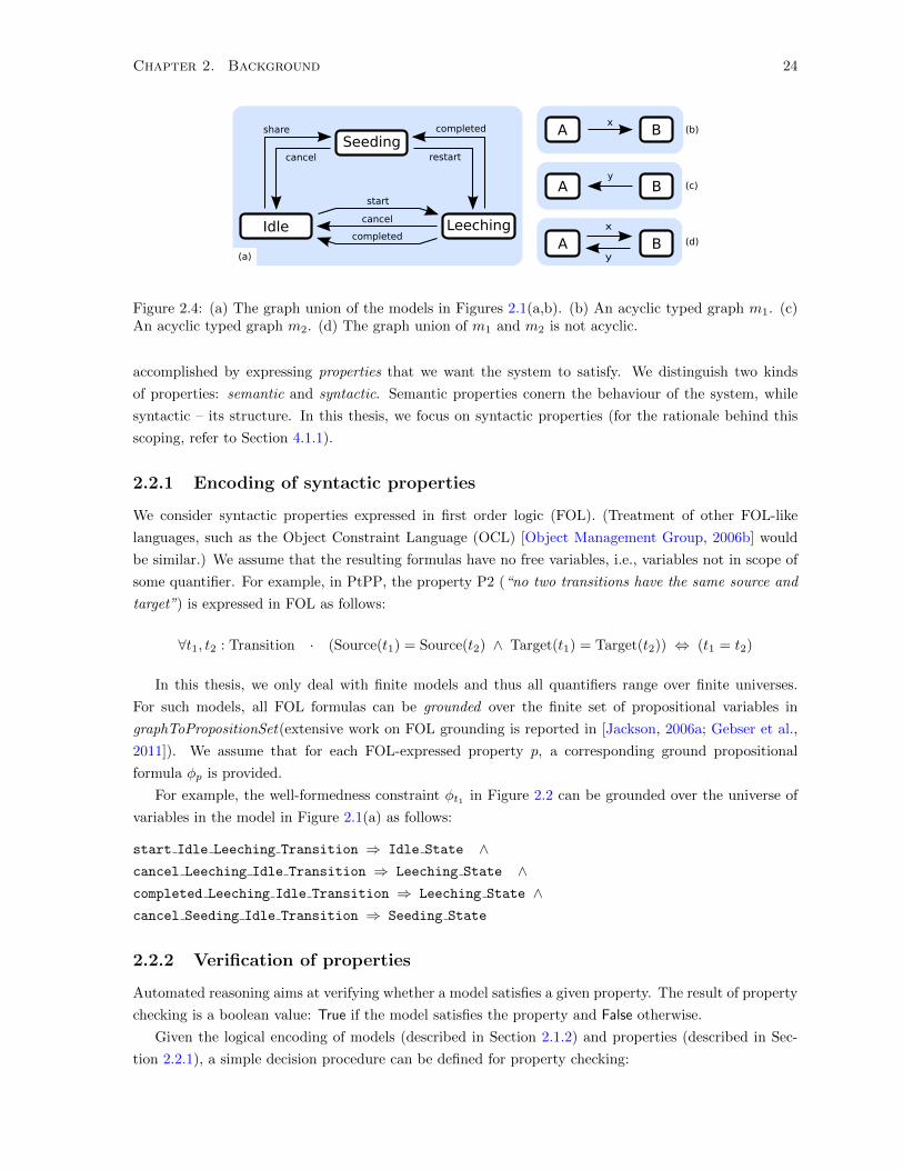
Chapter 2. Background 24
Leeching
completed
restartSeeding
Idle
start
cancel
completed
cancel
share Ax
B
Ay
B
A Bx
y(a)
(b)
(c)
(d)
Figure 2.4: (a) The graph union of the models in Figures 2.1(a,b). (b) An acyclic typed graph m1. (c)An acyclic typed graph m2. (d) The graph union of m1 and m2 is not acyclic.
accomplished by expressing properties that we want the system to satisfy. We distinguish two kinds
of properties: semantic and syntactic. Semantic properties conern the behaviour of the system, while
syntactic – its structure. In this thesis, we focus on syntactic properties (for the rationale behind this
scoping, refer to Section 4.1.1).
2.2.1 Encoding of syntactic properties
We consider syntactic properties expressed in first order logic (FOL). (Treatment of other FOL-like
languages, such as the Object Constraint Language (OCL) [Object Management Group, 2006b] would
be similar.) We assume that the resulting formulas have no free variables, i.e., variables not in scope of
some quantifier. For example, in PtPP, the property P2 (“no two transitions have the same source and
target”) is expressed in FOL as follows:
∀t1, t2 : Transition · (Source(t1) = Source(t2) ∧ Target(t1) = Target(t2)) ⇔ (t1 = t2)
In this thesis, we only deal with finite models and thus all quantifiers range over finite universes.
For such models, all FOL formulas can be grounded over the finite set of propositional variables in
graphToPropositionSet(extensive work on FOL grounding is reported in [Jackson, 2006a; Gebser et al.,
2011]). We assume that for each FOL-expressed property p, a corresponding ground propositional
formula φp is provided.
For example, the well-formedness constraint φt1 in Figure 2.2 can be grounded over the universe of
variables in the model in Figure 2.1(a) as follows:
start Idle Leeching Transition ⇒ Idle State ∧cancel Leeching Idle Transition ⇒ Leeching State ∧completed Leeching Idle Transition ⇒ Leeching State ∧cancel Seeding Idle Transition ⇒ Seeding State
2.2.2 Verification of properties
Automated reasoning aims at verifying whether a model satisfies a given property. The result of property
checking is a boolean value: True if the model satisfies the property and False otherwise.
Given the logical encoding of models (described in Section 2.1.2) and properties (described in Sec-
tion 2.2.1), a simple decision procedure can be defined for property checking:

Chapter 2. Background 25
Definition 2.5. Given a model m and a property p, with propositional encodings φm and φp respectively,
we check whether the expression φm ∧φp is satisfiable using a SAT solver. If φm ∧φp is satisfiable, then
m satisfies p and we write m |= p.
2.3 Model Transformations
2.3.1 Graph rewriting
Model transformations have been described as the “heart and soul of model-driven software develop-
ment” [Sendall and Kozaczynski, 2003]. Put simply, a model transformation is a model that describes
how to change other models. There are numerous approaches and languages for creating and executing
model transformations [Czarnecki and Helsen, 2006], however in this thesis we focus on a particular class
of transformations that relies on graph rewriting called graph transformations [Ehrig et al., 2006]. Such
transformations apply to models such as the model ma in Figure 2.5(a)2. They are implemented by
executing a set of graphical rules defined as follows:
Definition 2.6 (Transformation rule). A transformation rule R is a tuple R = 〈{NAC},LHS,RHS〉,where the typed graphs LHS and RHS are respectively called the left-hand and the right-hand sides of
the rule, and {NAC} represents a (potentially empty) set of typed graphs, called negative application
conditions.
To illustrate this we use models and transformations from the example scenario SolvEx, described
in more detail Section 5.1. Specifically, we use the example of a transformation that implements the
Encapsulate Variable refactoring [Casais, 1994]. A generic method for implementing this refactoring
using graph transformations was described by Mens et al. [Mens et al., 2005]. A simplified version of
this rule, called REV , is shown in Figure 2.5(e). The left-hand side (LHS) of the rule matches a node
a (and its associated edges such as ao:owner) that represents a public attribute . The right-hand side
(RHS) makes it private (by deleting the isPublic edge apt from a to True and adding a new isPublic
edge apf from a to False). It also creates a public getter operation ge and its associated edges. In
addition, the rule has two negative application conditions (NACs), i.e., conditions under which the rule
should not be applied. These are: NAC1, specifying the case when the class containing the public
attribute is an inner class, and NAC2, specifying the case when the class already has a getter.
The LHS, RHS and NACs of a rule consist of different parts, i.e., sets of model elements which do
not necessarily form proper graphs. These parts play different roles during the rule application:
Cr: The set of model elements that are present both in the LHS and the RHS, i.e., remain unaffected
by the rule.
Dr: The set of elements in the LHS that are absent in the RHS, i.e., deleted by the rule.
Ar: The set of elements present in the RHS but absent in the LHS, i.e., added by the rule.
Nr: The set of elements present in any NAC, excluding those included in Cr.
The parts of the example ruleREV are shown in Figure 2.6. Specifically, Cr is the set1 {a, ao, an, at, c1, ct},Dr is the (unary) set {apt}, Ar is {g, go, gn, gp, gt, apf}, and Nr is {g, gn, go, gt, c1n, c2}.
A rule R is applied to a model m by finding a matching site of its LHS in m:
2The model ma is shown in the abstract syntax of the Simplified UML Class Diagram metamodel defined in Fig-ure 2.5(d).
2Nodes that represent values (e.g., boolean True, the string N, etc.) are also considered to be part of Cr but are omittedfor brevity.

Chapter 2. Background 26
(b)
eo:owner
e:Attribute String:Class
ept:isPublicTrue:Bool
et:Type
Solver:Class
"effect":String
en:name
SolverException:Class
mb
eo:owner
e:Attribute String:Class
ept:isPublicTrue:Bool
et:Type
Solver:Classsn:nestedIn
"effect":String
en:name
SolverException:Class
ma
(a)
mc
(c)Solver:Class
sn:nestedIn
go:owner
ge:Operation
eo:owner
e:Attribute String:Class
TrueFalseepf:isPublic
et:Type gt:Type
gp:isPublic
SolverException:Class
"effect":String
en:name
"getEffect":String
gn:name
RHS
apf:isPublic
c1:Class
ct:Class
False
ao:owner
at:type
N:String
an:name
a:Attribute
True
gp:isPublic
go:owner
gt:type
"get"+N:String
g:Operation
gn:nameNAC2
True
c1:Class
ct:Classgp:isPublic
go:owner
gt:type
"get"+N:String
g:Operation
gn:name
c2:Classc1:Class
c1n:nestedInNAC1
apt:isPublic
c1:Class
ct:Class
True
ao:owner
at:type
N:String
an:name
a:Attribute
LHS
(e)
Attribute
isPublic
type
nestedIn
owner
isPublic
Class
Bool
String
name
name
Operation
type
owner
(d)
Figure 2.5: (a, b) Simplified UML Class Diagram models ma and mb. (c) Model mc resulting fromthe application of REV to mb. (d) Simplified UML Class Diagram metamodel. (e) Transformation ruleREV for doing the Encapsulate Variable refactoring.
Definition 2.7 (Matching site). A matching site of a transformation rule R in a model m is a tuple
K = 〈N,C,D〉, where C and D are matches of the parts Cr and Dr of the LHS of R in m, and N is
the set of all matches of NACs in m that are anchored at the matches C and D.
For example, a matching site K1 for the rule REV in the model ma in Figure 2.5(a) is 〈C1, N1, D1〉,where C1 = {e, eo, en, et, SolverException, String}, N1 = {{Solver, sn}}, and D1 = {ept}.
In the above definition, N denotes the set of all matches within m of the NACs of R. Given
the match of Cr and Dr. If the same NAC can match multiple ways, then all of them are included
in N as separate matches. For example, if the model in Figure 2.5(a) had another class Solver2
that also nested SolverException via an edge sn2, then N would contain two matches for NAC1:
N= {{Solver,sn},{Solver2,sn2}}. The set of matching sites define the places in the model m where
the rule can potentially be applied.
Definition 2.8 (Applicability condition). Given a transformation rule R, a model m, and matching
site K = 〈N, C, D〉, the rule R is applicable at K iff N is empty4.
4The theory of graph transformation requires some additional formal preconditions, most notably the gluing condi-tion [Ehrig et al., 2006]. In the following we always assume that these are satisfied.

Chapter 2. Background 27
Figure 2.6: Parts of the rule REV . Each rule part contains only those elements whose label appears inbold serif font2.
The above definition ensures that the rule can only be applied at a given site if no NAC matches. For
REV , the matching site K1 in ma does not satisfy the applicability condition as N1 6= ∅. On the other
hand, the model mb in Figure 2.5(b) contains a matching site K2 = 〈∅, C1, D1〉, which does satisfy this
condition. Then, the rule can be applied:
Definition 2.9 (Rule application). Given a transformation rule R, a model m, and a matching site K
in m for which the rule applicability condition is satisfied, rule R is applied, producing a model m′, by
removing D from m and adding A, where A is a match of the part Ar of R in m. Rule application is
denoted as mR
=⇒ m′.
Applying REV to mb at K2 thus requires the deletion of the element ept because it is contained in
D, and the addition of new elements according to Ar. The resulting model mc is shown in Figure 2.5(c),
where A is the set {ge, go, gn, gp, gt, epf}.We refer to rules such as the ones described above as “classical” to differentiate them from their
“lifted” counterparts which are discussed in Chapter 5.
2.3.2 Properties of transformations
A graph rewriting system (GRS) is a set of graph rewriting rules plus an input model. A GRS defines
a particular setting in which graph-rewriting-based model transformations take place. Graph rewrit-
ing systems are characterized by two important properties, namely, confluence and termination. The
definitions in this section are based on [Nupponen, 2005; Ehrig et al., 2006].
In the following, given a set of graph rewriting rules S, we denote the application of any rule in S
with the symbol “S
=⇒”. Repeated application of rules from S is denoted with the symbol “S∗=⇒”.
Consider the toy example model C1, shown in Figure 2.7(a), which contains three Classes: Pop,
Soda, and Coke. The rule F1, shown in Figure 2.7(e) transforms every Class x to a new Table, deleting
x. Applying the rule F1, shown in Figure 2.7(e) to C1, results in the model C2, shown in Figure 2.7(b),
which only contains Table elements. Since C2 no longer contains any Classes, the rule F1 can no longer
be applied to it. In contrast, consider the rule F2, shown in Figure 2.7(f), which transforms every Class
x to a new Table, without deleting x. Applying F2 to C1 results in the model C3, shown in Figure 2.7(c),
which contains the new Tables, as well as the original classes. F2 can therefore be applied again to C3,
resulting in the model C4, shown in Figure 2.7(d). C4 contains all elements of C3, as well as new copies

Chapter 2. Background 28
u: Class
LHS
v: Classuv: Table
RHS
x: Class
LHS
x: Table
RHS
x: Class
x: Class
LHS
x: Table
RHS
Pop : Table
Soda : Table
Coke : Table
Pop : Class
Soda : Class
Coke : Class
Pop : Table
Soda : Table
Coke : Table
Pop : Class
Soda : Class
Coke : Class
Pop : Class
Soda : Class
Coke : Class
Pop : Table
Soda : Table
Coke : Table
Pop : Table
Soda : Table
Coke : Table
(a) (b) (c) (d)
(e) (f) (g)
PopSoda : Table Coke : Class
PopCoke : Table Soda : Class
(h)
(i)
Figure 2.7: (a) Model C1. (b) Model C2, resulting from applying F1 to C1. (c) Model C3, resultingfrom applying F2 to C1. (d) Model C4, resulting from applying F2 to C3. (e) Transformation rule F1.(f) Transformation rule F2. (g) Transformation rule F3. (h) Model C5, resulting from applying F3 toC1. (i) Model C6, resulting from applying F3 to C1.
of all three Tables. It is thus possible to repeatedly apply F2, adding new copies of Tables ad infinitum.
The GRS 〈{F1}, C1〉 is called terminating, whereas the GRS 〈{F2}, C1〉 is called non-terminating.
We define termination for a GRS with as follows:
Definition 2.10 (Termination). Given a set S of graph rewriting rules and an input model m0, the
GRS G = 〈S,m0〉 is terminating iff there is no infinite sequence of rule applications m0S
=⇒ m1S
=⇒. . .
S=⇒ . . ..
Consider now the rule F3, shown in Figure 2.7(g), which merges two Classes u, v to a single Table
uv. There are three matching sites of F3 in C1: k1=(Pop, Soda), k2=(Pop, Coke), and k3=(Soda,
Coke). Depending on which matching site in C2 we apply F3 first, we get different models. For example,
applying it to k1 results in the model C5, shown in Figure 2.7(h), which contains the Table PopSoda
and the Class Coke; however, applying it to k2 results in the model C6, shown in Figure 2.7(i), which
contains the Table PopCoke and the Class Soda. For GRSs with multiple rules, the choice of which
rule to apply is an additional source of non-determinism. In contrast, it does not matter in what order
we find matching sites of F1 in C1: the result is always the model C2. The GRS 〈{F1}, C1〉 is called
confluent, whereas the GRS 〈{F3}, C1〉 is called non-confluent.
We define confluence for a GRS as follows:
Definition 2.11 (Confluence). Given a set S of graph rewriting rules and an input model m0, the GRS
G = 〈S,m0〉 is confluent iff for all models m1, m2 such that m0S∗=⇒ m1 and m0
S∗=⇒ m2, there is a
model mh such that m1S∗=⇒ mh and m2
S∗=⇒ mh.
2.4 Model-Driven Architecture
The Model Driven Architecture (MDA) [Object Management Group, 2014] is a software development
methodology introduced by the Object Management Group (OMG) in 2001. Relying on a series of
OMG standards, such as the Meta Object Facility (MOF) [Object Management Group, 2006a], the
Unified Modeling Language (UML) [Object Management Group, 2015a], the XML Metadata Interchange

Chapter 2. Background 29
(XMI) [Object Management Group, 2015b], and others, the MDA is OMG’s canonical realization of
Model Driven Engineering (MDE).
In MDA, models, metamodels and model transformations are first class development artifacts. Soft-
ware applications are created by applying transformations on models expressed at a high level of ab-
straction to derive models at lower levels of abstraction.
MDA promotes separation of concerns by adopting a design pattern whereby developers separate
the functionality of a system from the resources on which it depends in order to deliver it. A coherent
set of such resources is called a “platform”. Concerns are separated in the sense that developers can
create “Platform Independent Models” (PIMs), that abstract away the details of the platform. Then,
using transformations that take PIMs and platform models as inputs, they can derive “Platform Specific
Models” (PSMs) that include the additional necessary details at a lower level of abstraction.
Levels of abstraction are captured as “architectural layers”. The PIM/PSM pattern reflects the
crossing of the boundary between consecutive layers. Three such layers are defined:
(1) the layer of business or domain models,
(2) the layer of logical system models, and
(3) the layer of implementation models.
Transformations are used both to cross architectural layer boundaries, as well as to derive different
models within the same layer, such as models for analysis, documentation, etc.
In the first layer, developers model the relevant parts of real world, without worrying about how its
elements will be represented in the software system. Since this is the top layer, its models are known as
“Computation Independent Models” (CIMs).
Models in the second layer capture the high level architecture of the software system: its parts and
the interactions between them. Logical system models are PSMs with respect to CIMs. Specifically,
they are derived from the business layer using transformations that take as input CIMs and a set of
design decisions (which constitute the “platform” for this layer).
The third layer contains models that describe particular software artifacts, with enough information
such that they can functionally achieve the goals of the application. Implementation models are PSMs
with respect to logical system models. Specifically, they are derived from the second layer using transfor-
mations that take as input the logical system models, and a description of the implementation platform.
Typical examples of such transformations are code generators.
Consider the example of an application for managing hotel bookings. At the business level, developers
create CIMs that describe domain concepts such as rooms, dates, customers, etc. The CIMs are platform
independent with respect to logical system models in the next layer, since they do not contain information
such as client/server architectures, abstract data types, etc. The logical system models themselves are
platform independent compared to implementation models, that describe the Java source code realizing
the system.
2.5 Summary
In this chapter, we have introduced definitions and concepts that form the foundation for the techniques
presented in the rest of the thesis. We provided definitions for models and metamodels, which are used

Chapter 2. Background 30
throughout the thesis. The propositional encoding of models in particular is used in Chapters 4 and 6.
We also introduced the basics of model verification, which are used in Chapter 4. The theory of graph-
rewriting based model transformations is the basis for the technique presented in Chapter 5. Finally,
the description of Model Driven Architecture is used in Chapter 7.

Chapter 3
Representing Uncertainty
In this chapter, we describe how design-time uncertainty can be represented using partial models. We in-
troduce the formal semantics of partial models and describe equivalent reduced forms which can represent
the same set of concretizations but are best suited for different developer activities (human modelling
and comprehension; automated reasoning). We describe in detail the notation of the partial modelling
language, along with the rationale behind its design. We define a process of partialization through which
existing modelling languages can be adapted to support partial modelling and evaluate the notation
using an established theory for designing graphical modelling languages, called “Physics of Notations”.
Finally, we give an algorithm for constructing partial models from a set of concrete models. This way,
a developer who is faced with uncertainty about which alternative model she should use can create a
partial model that exactly and compactly encodes the set of available solutions.
We use the example PtPP scenario introduced in Chapter 1, whereby a team of developers is designing
a peer-to-peer system and is uncertain about certain decisions, as shown in Figure 1.2(a). The developers
explicate their uncertainty using the partial model shown in Figure 1.3, which encodes the six possible
resolutions of uncertainty shown in Figure 1.4.
The rest of this chapter is organized as follows: in Section 3.1 we define the formal semantics of
partial models. In Section 3.2 we give a complete description of the partial modelling notation, describe
how to adapt existing modelling languages to support it, and evaluate it using the “Physics of Notations”
theory. In Section 3.3 we introduce two reduced forms, i.e., equivalent representations of partial models.
In Section 3.4 we give the algorithm for constructing a partial model from a set of non-partial models.
We discuss related work in Section 3.5, and summarize and conclude in Section 3.6. Proofs of theorems
are found in Appendix A.1.
The contents of Sections 3.1, 3.3, 3.4, and 3.5 have been published in [Famelis et al., 2012] and
expanded in the manuscript [Famelis et al., 2015c], currently under review. The contents of Section 3.2
also expand on previously published material [Famelis, M. and Santosa, S., 2013].
3.1 Semantics
In this section, we formally define partial models and their associated operations. Semantically, a partial
model represents a set of classical (i.e., non-partial) models. The particular type of partiality we consider
in this paper is the one that allows a modeler to express uncertainty as to whether particular model
31

Chapter 3. Representing Uncertainty 32
atoms should be present in the model. The model is accompanied by a propositional formula, called the
May formula, which explicates allowable combinations of such atoms.
Definition 3.1. A Partial Model is a tuple 〈GT , ann, φ〉, where GT = 〈〈V,E, s, t〉, type, T 〉 is a typed
graph, ann : V ∪ E → {True,Maybe} is a function for annotating atoms in G, and φ is a propo-
sitional May formula over the set of propositional variables of Maybe-annotated atoms, i.e., the set
{atomToProposition(a)|a ∈ V ∪ E ∧ ann(a) = Maybe}.
In the above definition, an annotation True means that the atom must be present in the model,
whereas Maybe indicates uncertainty about whether the atom should be present. In other words, a
partial model consists of a typed graph whose atoms are annotated with True or Maybe, and a May
formula that describes the allowed configurations of its atoms.
Model Mp2p in Figure 1.3 is an example of a partial model. The atoms decorated with the seven-
pointed star icons, such as the state Finishing and the transition label completed(), are Maybe elements.
Atoms annotated with True, e.g., the state Idle and the transition action start, do not have special
decorations. Mp2p is accompanied by the May formula Φp2p shown below it in the figure. We have used
shorthand aliases to stand in for the full names of the propositional variables that correspond to Maybe
atoms. For example, Fs is an alias for the variable Finishing State.
Given a partial model M , we can obtain a classical model m by making a choice to keep or discard
each Maybe-annotated atom while satisfying the May formula constraint:
Definition 3.2. A concretization m of a partial model M = 〈G, ann, φ〉 is a well-formed classical model
such that
• ∀a ∈ m⇒ a ∈ G;
• φ′ = True, where φ′ is obtained by substituting all variables in φ using the rule:
– a ∈ m : φ[True/atomToProposition(a)], i.e., replace a’s encoding by True; and
– a 6∈ m : φ[False/atomToProposition(a)], i.e., replace a’s encoding by False.
For example, the concretizations of Mp2p are the models shown in Figures 1.4(a-f).
We define the semantics of partial models as follows:
Definition 3.3. Given a partial model M , we define its semantics as the set of all concretizations that
can be derived from it using Definition 3.2. We denote this set as C(M). If C(M) is empty, we say that
M is inconsistent.
In the PtPP example, C(Mp2p ) consists of the models shown in Figures 1.4(a-f).
In what follows, we only assume consistent partial models.
An important characteristic of partial models is that the size of the set of concretizations reflects
the modeler’s degree of uncertainty. A classical model has no uncertainty and uniquely corresponds
to a partial model with a single concretization (the uniqueness follows from Theorem 3.5, given in
Section 3.4).
Definition 3.4. A singleton partial model is a partial model M whose set of concretizations C(M)
contains exactly one concretization.
Chapter 3. Representing Uncertainty 33
Using partial model semantics, we can apply a formal approach to changing the degree of uncertainty
in a model, through a process of refinement:
Definition 3.5. Given two partial models M1 and M2, we say that M2 refines M1 (or that M1 is more
abstract than M2), denoted M2 �M1, iff C(M2) ⊆ C(M1), and M2 is consistent.
For example, the model M¬P2p2p in Figure 3.4(a) is more refined than Mp2p in Figure 1.3. In par-
ticular, C(Mp2p) consists of the models in Figure 1.4(a)-(f), whereas C(M¬P2p2p ) consists just of those in
Figure 1.4(c,d). Thus, M¬P2p2p has less uncertainty. We discuss the pragmatics of refinement in Chapter 6.
Given a partial model M , Definition 3.5 allows us to construe its concretizations as the ultimate
result of a series of refinements.
Lemma 3.1. Given a partial model M , each concretization mi ∈ C(M) corresponds uniquely to a
singleton partial model Mi such that C(Mi) = {mi}. Obviously, Mi �M .
In the following, we don’t make the distinction between a concretization and its corresponding sin-
gleton partial model and abbreviate this to mi �M .
Lemma 3.1 allows us to provide an alternative definition of partial model semantics in terms of the
refinement relationship.
Definition 3.6. The semantics of a partial model M is the set of all non-partial models mi such that
mi �M .
3.2 Notation
We introduced the partial model notation in Section 1.4.1. We give the full description below:
1. A partial model consists of two parts: a diagram and a May formula.
2. Elements of the diagram that are annotated with Maybe are decorated with a special icon (a black
seven-pointed star) which contains a propositional variable in white font used to represent the
proposition “the element is part of the model”.
3. The star decoration is placed on top or near its corresponding Maybe element, depending on its
concrete syntax. Specifically, it is placed:
• at the border of node elements,
• on top of vertex elements, and
• next to elements that are labels.
4. Elements that are annotated with True have no special decorations.
5. The May formula is placed either below or next to the diagram.
6. The May formula is expressed in the language of propositional logic, that uses propositional vari-
ables, logical connectives (And (∧), Or (∨), Not (¬), Biconditional (⇔), etc.) and parentheses.
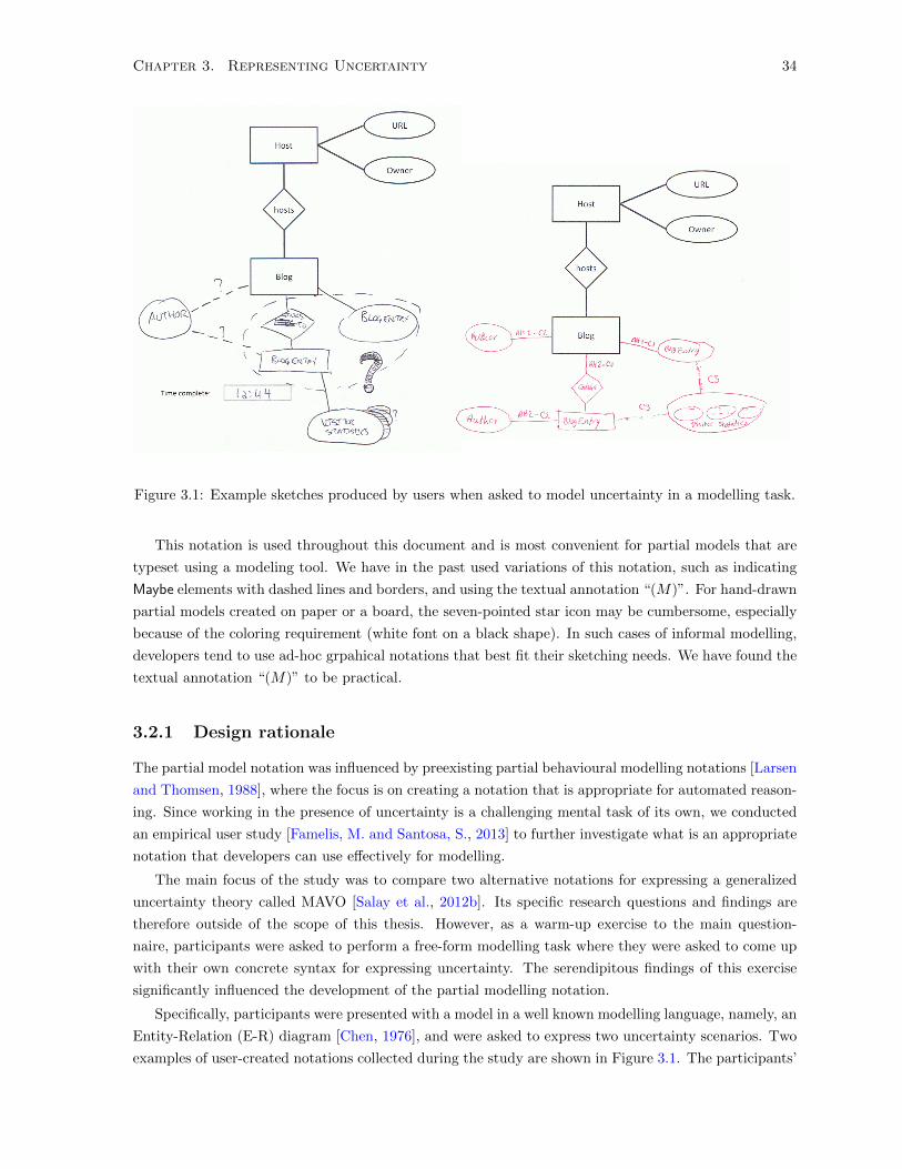
Chapter 3. Representing Uncertainty 34
Figure 3.1: Example sketches produced by users when asked to model uncertainty in a modelling task.
This notation is used throughout this document and is most convenient for partial models that are
typeset using a modeling tool. We have in the past used variations of this notation, such as indicating
Maybe elements with dashed lines and borders, and using the textual annotation “(M)”. For hand-drawn
partial models created on paper or a board, the seven-pointed star icon may be cumbersome, especially
because of the coloring requirement (white font on a black shape). In such cases of informal modelling,
developers tend to use ad-hoc grpahical notations that best fit their sketching needs. We have found the
textual annotation “(M)” to be practical.
3.2.1 Design rationale
The partial model notation was influenced by preexisting partial behavioural modelling notations [Larsen
and Thomsen, 1988], where the focus is on creating a notation that is appropriate for automated reason-
ing. Since working in the presence of uncertainty is a challenging mental task of its own, we conducted
an empirical user study [Famelis, M. and Santosa, S., 2013] to further investigate what is an appropriate
notation that developers can use effectively for modelling.
The main focus of the study was to compare two alternative notations for expressing a generalized
uncertainty theory called MAVO [Salay et al., 2012b]. Its specific research questions and findings are
therefore outside of the scope of this thesis. However, as a warm-up exercise to the main question-
naire, participants were asked to perform a free-form modelling task where they were asked to come up
with their own concrete syntax for expressing uncertainty. The serendipitous findings of this exercise
significantly influenced the development of the partial modelling notation.
Specifically, participants were presented with a model in a well known modelling language, namely, an
Entity-Relation (E-R) diagram [Chen, 1976], and were asked to express two uncertainty scenarios. Two
examples of user-created notations collected during the study are shown in Figure 3.1. The participants’
Chapter 3. Representing Uncertainty 35
sketches can be seen in the lower part of the figure.
In the left sketch, we can see that the participant has used dashed lines and question marks to
indicate uncertainty in the model. The participant has tried to indicate points of uncertainty using
grouping: a cluster of BlogEntry elements have been enclosed in a dashed lasso line, annotated with a
question mark. A second cluster of stacked elements named VisitorStatistics is dependent on the
first cluster. Additionally, a pair of dashed links to the Author element seem to be alternatives to each
other, and the choice seems to also be dependent on the existence of the BlogEntry cluster.
In the right sketch, the participant has avoided changing the E-R diagram notation, with the excep-
tion of the VisitorStatistics elements, that are drawn using dashed lines and ellipses. The participant
has tried to indicate the uncertainty in the model by annotating the different model elements with num-
bered choices (indicated by the letter C) and numbered alternatives (indicated by “Alt”). For example,
the entity Author appears twice: once connected to Blog (annotated as alternative #1 of choice #2)
and once connected to BlogEntry (annotated as alternative #2 of choice #2).
We note two themes: (a) the participants tried to express uncertainty by extending the existing
concrete syntax, and (b) they avoided using mathematical or logical formulas, and instead came up
with ad-hoc ways to enumerate alternatives on the model and their dependencies. These themes are
consistent with research in the field of feature modelling, where it has been shown that many useful
propositional formulas can be efficiently created graphically by humans [Czarnecki and Wasowski, 2007].
We thus chose to create a partial modelling notation that only minimally alters the concrete syntax
of the underlying language. We chose to use the seven-pointed star icon in order to avoid as much as
possible confusion with potential existing graphical symbols of underlying languages (more on this in
Section 3.2.2) because it is a symbol rarely used in graphical modelling languages (to our best knowledge,
there is no graphical language for modelling software artifacts that uses it).
We also developed a purely graphical language for expressing logical dependencies between Maybe
elements without using the language of propositional formulas. In this, we were guided by the principles
described by D. Moody’s “Physics of Notations” theory [Moody, 2009], with the aim to maximize the
effectiveness of the notation for reading and writing tasks. Even though we have evidence [Famelis,
M. and Santosa, S., 2013] that this language is more usable for expressing and comprehending partial
models, it has limited (logical) expressiveness and is difficult to use when manipulating partial models
(e.g., when applying transformations, as described in Chapter 5). We therefore do not use it in the
examples in this dissertation. Nonetheless, it was very influential in the development of the graphical
tool Mu-Mmint, which is described in Chapter 7.
3.2.2 Base language metamodel adaptation
Our approach for representing uncertainty is modelling-language independent, in the sense that it allows
uncertainty to be captured in any model that is expressed in a modelling language defined using a
metamodel [Atkinson and Kuhne, 2003; Object Management Group, 2006a]. In effect, the language of
partial models is an annotation language that can be superimposed on any graphical modelling language.
In this section, we describe the process by which the metamodel of any existing modelling language can
be adapted for partial modelling, such that it can be used in modelling tools.
In a given modelling scenario, we call the modelling language of the models without uncertainty the
“base language”. In the PtPP example, the developers are working with UML state machines, thus the
base language is the one defined by the metamodel in Figure 1.2(c).

Chapter 3. Representing Uncertainty 36
Box
Box
+ isMaybe : Boolean
0..5contains
*contains
0..1
*
b:Box
a:Box
c:Box
MayFormula
+ formula : String
1y
x ¬y
x
Figure 3.2: (a) Simple Box metamodel B, (b) partialized Box metamodel Bp, (c) partial model, instanceof Bp, that violates the multiplicity constraints of B.
Given a base modelling language, we derive its corresponding partial language through a process
which we call metamodel partialization.
Definition 3.7. Given a base language metamodel MB, its corresponding partial metamodel MP , called
a partialized metamodel, is a metamodel that contains the same meta-elements as MB, with the following
adaptations:
• Every meta-element has an additional boolean meta-attribute isMaybe.
• MP contains an additional singleton meta-class MayFormula, that has a single attribute formula.
• The multiplicity constraints of every meta-association are unbounded (typically denoted by “*”).
The boolean meta-attribute isMaybe is used to represent the annotation function ann in Defini-
tion 3.1. Specifically, for each instance element e for which ann(e) = Maybe, the meta-attribute is set to
True; otherwise, it is set to False.
The meta-class MayFormula is used to store the partial model’s propositional May formula in its
attribute formula. It is a singleton class (i.e., it has exactly one instance) since a partial model can only
have one May formula. We have intentionally not prescribed a specific data type for this attribute. A
String is sufficient; however, toolsmiths may choose to use more sophisticated data structures such as
Binary Decision Diagrams (BDDs) [Akers, 1978] or languages specifically tailored for representing logic,
such as SMT-LIB [Barrett et al., 2010].
To motivate the need to relax multiplicity constraints of meta-associations, consider for example the
simple metamodel B shown in Figure 3.2(a) that defines a toy language for describing arrangements of
boxes. In this language, a Box can contain up to five other Boxes and can be contained in up to one
other Box. Consider also the partial model shown in Figure 3.2(c), that encodes a scenario where we
are uncertain whether the Box b should be contained in the Box a or the Box c. The uncertainty is

Chapter 3. Representing Uncertainty 37
Transition
Action
0..1
1
State
1
1
src
1
1
tgt
EntryAction
0..1
1
Transition Action**
State
*
*
src
*
*
tgt
EntryAction**
+ isMaybe : Boolean + isMaybe : Boolean
+ isMaybe : Boolean + isMaybe : Boolean
MayFormula
+ formula : String
1
Seeding
Idle
Leeching
/completed()
/completed()
Dt
Ba
Seeding:State
src
Idle:State
Leeching:State
tc:Transition
completed:Action
tgt tgtB D
Bt
Da
t
a
Figure 3.3: (a) Base language in PtPP: simplified UML State Machine metamodel. (b) Partial StateMachine metamodel. (c) Fragment from Mp2p. (d) A different way to model the same fragment that isexpressible in the abstract syntax but not in the concrete syntax (May formula not shown).
expressed by drawing two Maybe annotated containment edges originating from b and ending at a and
c, respectively. The May formula (an instance of the singleton meta-class MayFormula of Bp) enforces
that only one of the two edges can be included in concretizations. This partial model clearly violates the
multiplicity constraints of the metamodel B: the Box b has two containment associations, whereas it is
allowed to have at most one. On the other hand, its concretizations are well formed B models. Relaxing
the multiplicity constraints of the base language metamodel, as shown in the partial metamodel Bp in
Figure 3.2(b), allows expressing such scenarios without breaking metamodel conformance rules.
Not all instances of a partialized metamodel are consistent partial models, i.e., it is possible to
instantiate partial models that do not have any well-formed concretizations. Partial model editors
should therefore support consistency checking. This can be accomplished by combining the May formula
with the base language well-formedness constraints and checking the combination using a SAT solver.
In the following, we only consider consistent partial models.
It is also possible to instantiate consistent partial models that are not expressible in the concrete
syntax of the base language. This is especially true because of the unbounded multiplicities of the
partialized metamodel. For example, the result of metamodel partialization to the simplified UML State

Chapter 3. Representing Uncertainty 38
Machine metamodel used in PtPP, in Figure 3.3(b). We have copied in Figure 3.3(a) the metamodel
from Figure 1.2(c). The partial model in Figure 1.3 conforms to this partial metamodel. Consider the
model fragment of Mp2p shown in Figure 3.3(c), consisting of the state Leeching and the two Maybe-
annotated transitions on completed towards Idle and Seeding. Because the partialized metamodel
allows unbounded multiplicities, it is possible to model the same scenario using the arrangement of
Maybe elements shown in Figure 3.3(d). Specifically, instead of using two different Maybe-annotated
transitions, we have modelled the same scenario with a single Transition tc, that has two Maybe-
annotated tgt arrows to the two target states. This way of modelling the PtPP scenario might be
more intuitive to the modeller; however, it is not expressible in the concrete UML State Machine syntax
where Transitions are drawn as arrows themselves. This example demonstrates that the partial model
annotation language is versatile and can be used in whatever way is most intuitive to developers.
Definition 3.4 and Lemma 3.1 allow us to establish the correspondence between instances of the base
and partialized metamodels:
Theorem 3.1. Every well formed base language instance model can be uniquely transformed into a
singleton partial model, instance of the partialized metamodel, and vice versa.
Specifically, a base language instance can be transformed as an instance of the partialized metamodel
by adding a meta-attribute isMaybe to each element and setting it to True, and by including an instance
of the class MayFormula, with the formula attribute set to True. Conversely, every singleton partial
model, i.e., a (consistent) partial model that has exactly one concretization can be transformed as an
instance of the base language by dropping the isMaybe meta-attribute from each element and deleting
the instance of the MayFormula class. Since the partial model is consistent, its single concretization is
(by definition) well-formed with respect to the base language metamodel.
Using the partialization technique, existing modelling tools that support metamodelling can be
adapted to support partial models. We note that the objective of metamodel partialization is to aid the
creation of modelling software, not to set the mathematical foundation of partial models. Therefore, in
the rest of the thesis, we use the formalization of partial models as given in Definition 3.1.
3.2.3 Assessment
In this section, we assess the partial model annotation language using the theory of “Physics of Nota-
tions” [Moody, 2009], a design theory focused on creating cognitively effective visual notations. The
theory provides a comprehensive framework for evaluating the perceptual properties of graphical lan-
guages based on a set of well-defined design principles.
The results of our assessment are summarized below. For each principle, we assign a rating, ranging
from + + (“very good”) to - - (“very bad”). We additionally use +/- to mean “it depends”.
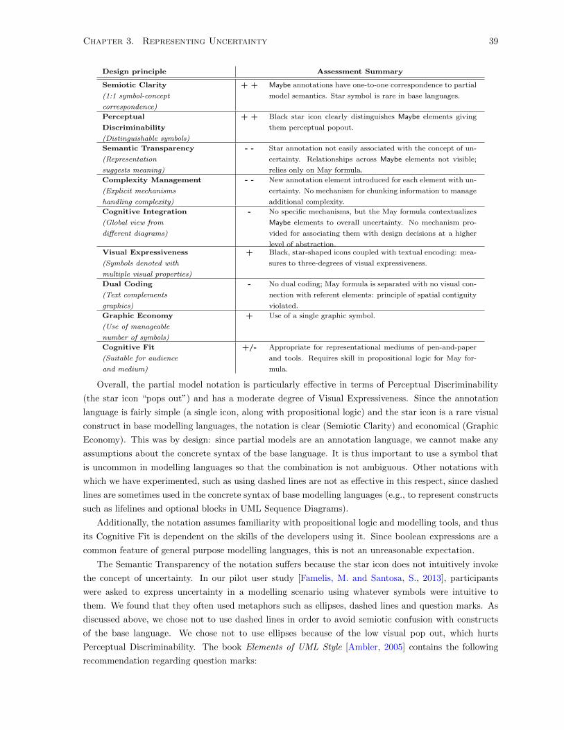
Chapter 3. Representing Uncertainty 39
Design principle Assessment Summary
Semiotic Clarity
(1:1 symbol-concept
correspondence)
+ + Maybe annotations have one-to-one correspondence to partial
model semantics. Star symbol is rare in base languages.
Perceptual
Discriminability
(Distinguishable symbols)
+ + Black star icon clearly distinguishes Maybe elements giving
them perceptual popout.
Semantic Transparency
(Representation
suggests meaning)
- - Star annotation not easily associated with the concept of un-
certainty. Relationships across Maybe elements not visible;
relies only on May formula.
Complexity Management
(Explicit mechanisms
handling complexity)
- - New annotation element introduced for each element with un-
certainty. No mechanism for chunking information to manage
additional complexity.
Cognitive Integration
(Global view from
different diagrams)
- No specific mechanisms, but the May formula contextualizes
Maybe elements to overall uncertainty. No mechanism pro-
vided for associating them with design decisions at a higher
level of abstraction.Visual Expressiveness
(Symbols denoted with
multiple visual properties)
+ Black, star-shaped icons coupled with textual encoding: mea-
sures to three-degrees of visual expressiveness.
Dual Coding
(Text complements
graphics)
- No dual coding; May formula is separated with no visual con-
nection with referent elements: principle of spatial contiguity
violated.
Graphic Economy
(Use of manageable
number of symbols)
+ Use of a single graphic symbol.
Cognitive Fit
(Suitable for audience
and medium)
+/- Appropriate for representational mediums of pen-and-paper
and tools. Requires skill in propositional logic for May for-
mula.
Overall, the partial model notation is particularly effective in terms of Perceptual Discriminability
(the star icon “pops out”) and has a moderate degree of Visual Expressiveness. Since the annotation
language is fairly simple (a single icon, along with propositional logic) and the star icon is a rare visual
construct in base modelling languages, the notation is clear (Semiotic Clarity) and economical (Graphic
Economy). This was by design: since partial models are an annotation language, we cannot make any
assumptions about the concrete syntax of the base language. It is thus important to use a symbol that
is uncommon in modelling languages so that the combination is not ambiguous. Other notations with
which we have experimented, such as using dashed lines are not as effective in this respect, since dashed
lines are sometimes used in the concrete syntax of base modelling languages (e.g., to represent constructs
such as lifelines and optional blocks in UML Sequence Diagrams).
Additionally, the notation assumes familiarity with propositional logic and modelling tools, and thus
its Cognitive Fit is dependent on the skills of the developers using it. Since boolean expressions are a
common feature of general purpose modelling languages, this is not an unreasonable expectation.
The Semantic Transparency of the notation suffers because the star icon does not intuitively invoke
the concept of uncertainty. In our pilot user study [Famelis, M. and Santosa, S., 2013], participants
were asked to express uncertainty in a modelling scenario using whatever symbols were intuitive to
them. We found that they often used metaphors such as ellipses, dashed lines and question marks. As
discussed above, we chose not to use dashed lines in order to avoid semiotic confusion with constructs
of the base language. We chose not to use ellipses because of the low visual pop out, which hurts
Perceptual Discriminability. The book Elements of UML Style [Ambler, 2005] contains the following
recommendation regarding question marks:
Chapter 3. Representing Uncertainty 40
“While you are modelling, you may discover that you do not have complete information. [...]
You should always try to track down a sufficient answer, but if you cannot do so immediately,
then make a good guess and indicate your uncertainty. [A] common way to do so [is using]
question marks.”
Question marks are therefore associated with specific semantics regarding the representation of uncer-
tainty: indicating provisional decisions. Overloading the symbol would thus risk creating confusion and
seriously harm Semiotic Clarity, especially since there are opposing underlying assumptions about how
to model uncertainty (the goal of partial modelling is to avoid making provisional decisions). Ultimately,
we chose to prioritize Semiotic Clarity and Perceptual Discriminability over Semantic Transparency, rea-
soning that the small learning curve (becoming familiarized with the meaning of one symbol) is not an
unreasonable trade-off for the elimination of ambiguity.
The simplicity of the language mitigates the need for Dual Coding. On the other hand, this simplicity
means that the notation lacks a good system for Complexity Management, which can be a problem as
more and more uncertainty is encoded in a model. Similarly, since the focus is on expressing uncertainty
in a single modelling artifact, there are no explicit Cognitive Integration mechanisms, especially in terms
of providing an explicit mechanism for mapping Maybe elements to design decisions (if a mechanism for
capturing them exists). In [Famelis, M. and Santosa, S., 2013] we experimented with grouping Maybe
elements based on the point of uncertainty with which they are associated. We further elaborated this
idea in [Famelis et al., 2015a], by further organizing Maybe elements based on which specific alternative
solution to a point of uncertainty they reify, as well as explicitly keeping track of points of uncertainty
and alternative solutions in a separate modelling artifact called “Uncertainty Tree”. Such organizational
mechanisms significally enhance Complexity Management and Cognitive Integration, and are effective
for modelling, reasoning and refining partial models. However, they are not well suited to changes caused
to a partial model due to transformations (discussed in Chapter 5) because transformations affect partial
models at a lower level of granularity, i.e., per element, thus negating the benefits of element groupings.
In this dissertation we aim to present all partial model operators, listed in Section 7.2. Therefore we use
the notation that is well suited for all of them.
3.3 Reduced Forms
There are multiple ways of representing a given set of classical models using partial models. For example,
consider the set of models S¬P2 consisting solely of the two models in Figures 1.4(c, d). These models
are the concretizations of Mp2p that violate the property P2: “no two transitions have the same source
and target”. There exist multiple partial models Mi for which C(Mi) = S¬P2. Figure 3.4 shows three
such examples. The model in Figure 3.4(a) has only two Maybe-annotated atoms and a May formula
Ca ⇔ Ct. The model in Figure 3.4(b) has all of its atoms annotated with Maybe but a more complex
May formula. Both partial models have the exact same set of concretizations S¬P2 but have different
combinations of Maybe annotations and May formulas. Figure 3.4(c) shows a model that contains both
Maybe-annotated and True-annotated elements. However, its May formula excludes two of the Maybe-
annotated elements (the transition from Leeching to Seeding and its corresponding action completed)
from all concretizations.
Definition 3.8. Two partial models M1, M2 are equivalent, denoted M1 ∼M2, iff they have the same
set of concretizations, i.e., C(M1) = C(M2). It holds that M1 ∼M2 iff M1 �M2 and M2 �M1.

Chapter 3. Representing Uncertainty 41
Seeding
Idle Leeching
/cancel()
/start()
/cancel()
/completed()
/share()
/restart()
Ct
Ca
Seeding
Idle Leeching
/cancel()
/start()
/cancel()
/completed()
/share()
/restart()
Ct
Dt
Aa
Ca
Da
At
May formula: Ca Ct
Si
Ss
SlKt
Ka
LtLa
May formula: At Aa Dt Da Kt Ka Lt La Mt Ma Si Ss Sl Λ (Ca Ct)
Seeding
Idle Leeching
/cancel()
/start()
/cancel()
/completed()
/share()
/restart()
/completed()
BtCt
Dt
Ba
Ca
Da
SlKt
Ka
LtLa
Mt
Ma
May formula: Dt Da Kt Ka Lt La Sl Λ ¬Bt ¬Ba (Ca Ct)
Figure 3.4: Some equivalent partial models that encode the set S¬P2, consisting of the two concretiza-tions in Figures 1.4(c, d): (a) in GRF (b) in PRF (c) containing two superfluous Maybe-annotated atoms(Bt and Ba).
To help represent models, we define two special forms: Graphical Reduced Form (GRF) and Propo-
sitional Reduced Form (PRF). Intuitively, a model in GRF represents most information in the graph,
whereas in PRF, it represents most of the information in the formula. For example, Figure 3.4(a,b) shows
the GRF and the PRF versions, respectively, of the model M¬P2e in Figure 3.4(c). GRF is the form used

Chapter 3. Representing Uncertainty 42
when a human works with a partial model while PRF is the form used for automated reasoning. We use
both forms in defining algorithms in Chapter 4.
We refer to constructing an equivalent GRF (PRF) of a partial model as “putting it to GRF (PRF)”.
In the following, the symbol “�” denotes logical entailment.
All algorithms construct models in their abstract syntax. We assume that putting models in their
concrete syntax is done automatically by modeling tools.
3.3.1 Graphical Reduced Form (GRF)
Definition 3.9. A GRF of a partial model M = 〈G, ann, φ〉 is a partial model
M GRF = 〈G GRF, ann GRF, φ GRF〉, such that M ∼M GRF and there does not exist M ′ ∼M , such that
M ′ has fewer Maybe-annotated atoms than M GRF.
A partial model can have many equivalent GRF models. All GRF equivalents have the same number
of Maybe-annotated atoms.
Algorithm 1 describes how to put an arbitrary partial model into its GRF form.
ALGORITHM 1: GRF Conversion.Input: A partial model M = 〈G, ann, φ〉Output: A GRF equivalent M GRF = 〈G GRF, ann GRF, φ GRF〉 of M
1 G GRF := G;
2 φ GRF := φ;3 B = backbone(φ);4 foreach atom a ∈ G do5 if ann(a) = Maybe then6 if atomToProposition(a) ∈ B then7 ann GRF(a) := True;
8 substitute φ GRF[True/atomToProposition(a)];
9 else if (¬atomToProposition(a)) ∈ B then10 remove a from G GRF;
11 substitute φ GRF[False/atomToProposition(a)];
12 end
13 end
14 end
15 return M GRF = 〈G GRF, ann GRF, φ GRF〉;
The algorithm works as follows: We first create a copy of the input model (Lines 1-2) and then
compute the backbone of its May formula (Line 3) – the set of propositional variables (negated and not)
that follow from it [Marques-Silva et al., 2010]. We treat this computation as a black-box. Next, we
look at each Maybe-annotated atom in the partial model: if it is in the backbone, then we annotate it
with True and set it to True in the May formula (Lines 6-8). If its negation is in the backbone, then we
remove it from the model altogether and set it to False in the May formula (Lines 9-11).
Given the backbone, the algorithm performs linearly in the number of Maybe-annotated atoms.
Therefore, the complexity of the algorithm is the complexity of the backbone computation, which is
NP-hard [Kilby et al., 2005].
In our example, the partial model in Figure 3.4(c) has the May formula Dt∧Da∧Kt∧Ka∧Lt∧La∧Sl∧¬Bt∧¬Ba∧ (Ca⇔ Ct). The backbone computation returns the set {Dt, Da, Kt, Ka, Lt, La, Sl,¬Bt,¬Ba}.

Chapter 3. Representing Uncertainty 43
Each of the atoms represented by the variables Dt, Da, Kt, Ka, Lt, La, Sl is annotated with True, and the
variables are substituted with True in φ. The atoms represented by Bt and Ba are deleted, and their
variables are substituted by False in φ. The resulting partial model is shown in Figure 3.4(a). Its May
formula is True ∧ True ∧ True ∧ True ∧ True ∧ True ∧ True ∧ ¬False ∧ ¬False ∧ (Ca⇔ Ct) which evaluates
to Ca⇔ Ct.
The following theorems state correctness of Algorithm 1.
Theorem 3.2. Let M be a partial model and M GRF be a result of applying Algorithm 1. Then,
M ∼M GRF.
Theorem 3.3. If M GRF is a model computed from M using Algorithm 1, then there does not exist a
M ′ ∼M such that M ′ has fewer Maybe-annotated atoms than M GRF.
3.3.2 Propositional Reduced Form (PRF)
Definition 3.10. A PRF of a partial model M = 〈G, ann, φ〉, is a partial model
M PRF = 〈G PRF, ann PRF, φ PRF〉 such that M ∼M PRF and G PRF only has Maybe-annotated atoms.
A partial model can have multiple PRF equivalent models.
Algorithm 2 describes how to put a given partial model into its PRF.
ALGORITHM 2: PRF ConversionInput: A partial model M = 〈G, ann, φ〉Output: A PRF equivalent M PRF = 〈G PRF, ann PRF, φ PRF〉 of M
1 G PRF := G;
2 φ PRF := φ;3 foreach atom a in G PRF do4 if ann(a) = True then5 ann PRF(a) := Maybe;
6 φ PRF := φ PRF ∧ atomToProposition(a);
7 end
8 end
9 return M PRF = 〈G PRF, ann PRF, φ PRF〉;
The algorithm works as follows: We first create a copy of the input model (Lines 1-2). Next, we find
all True-annotated atoms and (a) annotate them with Maybe and (b) conjoin their corresponding propo-
sitional variable to the May formula (Lines 4-6). The resulting model only contains Maybe-annotated
atoms. The algorithm is linear to the number of atoms of the model.
In our example, to compute the PRF of the GRF partial model in Figure 3.4(a), we annotate all True-
annotated atoms with Maybe and conjunct their respective propositional variable to the May formula.
The resulting PRF partial model is shown in Figure 3.4(b).
The following theorem states correctness of Algorithm 2.
Theorem 3.4. Let M be a partial model and M PRF be a result of applying Algorithm 2. Then,
M ∼M PRF and M has only Maybe-annotated atoms.

Chapter 3. Representing Uncertainty 44
3.4 Constructing Partial Models
In this section, we give an algorithm for constructing a partial model from a set of known alternatives
(Algorithm 3).
ALGORITHM 3: Construction of a partial model from a set of concrete models.
Input: Set A of concrete models of type TOutput: A partial model M , such that C(M) = A.
1 GTu := GraphUnion(A);
2 MayAtomsM := {a|a ∈ GTu ∧ ∃m ∈ A · a /∈ m};
3 foreach atom a ∈ GTu do
4 if a ∈ MayAtomsM then5 ann(a) := Maybe;6 else7 ann(a) := True;8 end
9 end10 φ :=False;11 foreach m ∈ A do
12φm :=
∧{atomToProposition(a)|a ∈ MayAtomsM , a ∈ m} ∧∧{¬atomToProposition(a)|a ∈ MayAtomsM , a /∈ m};
13 φ := φ ∨ φm;
14 end
15 return M = 〈GTu , ann, φ〉
Construction of partial models from a known set of models is achieved by merging their graphs and
annotating the atoms that vary between them by Maybe. Additionally, the May formula is constructed
to capture the allowable configurations of the Maybe atoms.
We capture this process in Algorithm 3 as follows:
1. To create a partial model M from a set A of classical models of type T , we first create the typed
graph GTu of their graph union (cf. Definition 2.4).
2. Next, we find every atom of GTu for which there exists at least one concretization in A that does
not contain it. We store all these atoms in the set MayAtomsM (Line 2). Every atom in GTu then
gets an annotation: if an atom is in MayAtomsM , it is annotated with Maybe; otherwise, it is
annotated with True (Lines 3-8).
3. We construct the May formula φ as a disjunction of conjunctions of Maybe-annotated atoms. We
initialize φ as False (Line 10) and iteratively add disjunctive clauses for each model m in A. More
specifically, given m, we create a conjunction φm of all MayAtomsM . If an atom a of MayAtomsM
does not exist in m, it appears in φm negated (Line 12). Ultimately, the May formula becomes the
disjunction of all the individual φm clauses (Line 13).
In the PtPP example, the six alternative behavioural designs in Figure 1.4(a-f) can be represented
using the partial model shown in Figure 1.3. For example, the state Finishing exists in only two
concretizations, and the transition on restart in three; therefore, both are represented as Maybe.
Atoms such as the state Idle are present in all concretizations, and thus are represented as True (i.e.,
without the star decoration). The corresponding May formula is shown at the bottom of Figure 1.3.

Chapter 3. Representing Uncertainty 45
The algorithm is linear in the total number of atoms and by construction creates a partial model
with a set of concretizations equal to the input set of models. We codify this in the following theorem.
Theorem 3.5. Applying Algorithm 3 to a set of classical models A results in a partial model M such
that C(M) = A.
The next theorem leads us to observe that Algorithm 3 can be used as a “brute-force” algorithm
to compute the GRF of a partial model, by first breaking the partial model down to its constituent
concretizations and then merging them again.
Theorem 3.6. Models generated in Algorithm 3 are in GRF.
In Section 4.3, we compare the relative efficiency of Algorithms 1 and 3 for putting a partial model
into GRF.
3.5 Related Work
The notion of design-time uncertainty used in this work is that of “multiple possibilities”. Thus, partial
models are a formalism where a set of models is encoded in a single modelling artifact. This is a
common abstraction pattern in software engineering, often used in cases where developers are required
to work with sets of related and/or similar models. Examples of formalisms that follow the same
abstraction pattern are metamodels, partial behavioural formalisms, and software product lines. Since
such formalisms implement the same abstraction pattern, and given that some of them have similar
expressive powers, it would be tempting to unify them in a single language. However, this would be
counter-productive because each of them has been conceived with a different intent in mind. The intent
of each formalism defines its assumed context of use and prioritizes what tasks are important for the
formalism to efficiently support its context. In the following, we briefly discuss the related formalisms
discussing their particular intended context of use, and compare them to partial models.
3.5.1 Metamodels
A metamodel is a model that defines the set of models which conform to it, similar to how a gram-
mar defines the set of acceptable phrases of a language. Metamodels are typically expressed using a
meta-metamodelling language such as MOF [Object Management Group, 2006a] and KM3 [Jouault and
Bezivin, 2006]. Additional constraints are typically expressed in a constraint language such as OCL [Ob-
ject Management Group, 2006b]. In principle, we could use a metamodel to express the set of possible
models from which a team has to choose in order to resolve their uncertainty. This would involve refining
the metamodel of the language used for development to one containing very specialized “singleton” types
of atoms. Such an approach would be very awkward, as it involves conceptually altering the development
language itself, the consequences of which may be hard to manage.
3.5.2 Partial behavioural models
A number of partial behavioural modelling formalisms have been studied in the context of abstraction
(for verification) or for capturing early design models [Fischbein et al., 2012].

Chapter 3. Representing Uncertainty 46
Modelling uncertainty in behavioural models Modal Transition Systems (MTSs) [Larsen and
Thomsen, 1988] allow introduction of uncertainty about transitions on a given event, whereas Disjunc-
tive Modal Transition Systems (DMTSs) [Larsen, 1991] add an additional constraint that at least one
of the possible transitions must be taken in the refinement. Restricted DMTSs (rDMTSs) [Ben-David
et al., 2013] is a variant of DMTSs that is closed under the merge for models of different vocabular-
ies. Incompletely and partially labelled transition systems (IPLTS) allow the definition of states that
represent parts of a system that are yet to be fully specified [Ghezzi et al., 2014]. These approaches
compactly encode an over-approximation of the set of possible LTSs and thus reasoning over them suffers
from information loss. Moreover, they employ refinement mechanisms that allow resulting LTS models
to have an arbitrary number of states. This differs from the treatment provided in this paper, where
we concentrated only on “structural” partiality and thus state duplication was not applicable. While
the intent of behavioural specification methods is the same as ours, partial models are applicable to
any kind of modelling language (not just behavioural models) that can be defined using a metamodel.
While we have used a state-machine-like language for the motivating example in this presentation, there
is nothing inherent in our approach that mandates it. For example, in Section 3.2.2, we applied our
approach to a toy custom structural language for describing arrangements of boxes. It has also been
applied to languages such as UML Class Diagrams [Famelis et al., 2013] and goal models [Salay et al.,
2012a].
Underspecification and Nondeterminism When specifying a system, scope defines what elements
are relevant to the system, and span – what level of abstraction is acceptable. Elements that are outside
the scope and span of the specification are ones the developer does not care about. Elements that are
within the scope and span, but are not present in the specification, are underspecified. In practice, this
is often used to indicate that these elements are to be re-visited at a later point when more information
becomes available. Thus, an underspecified system represents a set of fully specified possibilities. Non-
determinism is a common way to interpret underspecification in the context of behavioural modelling.
Underspecification is used to implicitly (through omission) hint at what developers are uncertain about.
On the contrary, partial modelling is used to explicitly define what the developers do not know. In
addition, partial modelling allows us to combine underspecification and explicit uncertainty. For ex-
ample, MTSs allow underspecification using non-determinism, while also having explicit utterances of
uncertainty.
3.5.3 Software product lines
Another relevant area is software product line (SPL) engineering [Pohl et al., 2005] where a product
line captures a family of models by identifying their commonalities and variabilities. The notion of a
feature is central in variability modelling, albeit informally defined (e.g., in the Feature Oriented Analysis
and Design (FODA) approach, a dictionary definition is used: “A prominent or distinctive user-visible
aspect, quality, or characteristic of a software system or systems” [Kang et al., 1990]). The main intent
of SPL engineering is therefore the strategic maintenance of a set of modelling artifacts that realize
high-level features, and that can be combined to create desirable products. In contrast, the intent of
uncertainty modelling is to facilitate decision deferral as discussed in Section 1. In fact, these two intents
can co-exist within the same modelling artifact. For example, a practitioner may be uncertain about
whether to include a feature in a product line. In the rest of this section we elaborate on the differences.

Chapter 3. Representing Uncertainty 47
Figure 3.5: An example product line, representing a family of vending machines. The product lineconsists of a Feature Model (left) and a Featured Transition System (right). Elements of the transitionsystem are annotated with presence conditions. Image source: [Classen et al., 2010].
Modelling variability Features are defined at an abstract level and are conceptually separate from the
software artifacts. Their expression in software models is done using variability points. Dependencies
between features are typically maintained in a separate Feature Model [Kang et al., 1990; Schobbens
et al., 2006]. Some approaches incorporate expressions of variability directly using notational extensions
in the metamodel [Morin et al., 2009]. In practice, however, the annotative approach is typically used,
where variability points take the form of presence conditions attached to model elements [Czarnecki
and Antkiewicz, 2005; Kastner and Apel, 2008]. These conditions are propositional expressions over
the vocabulary of features. They ensure that a model element is only included in a product if the
desired combination of features is selected. An example product line, taken from [Classen et al., 2010],
is shown in Figure 3.5. This product line represents a family of vending machines and consists of a
Feature Model (shown on the left) and a Featured Transition System (shown on the right). A Featured
Transition System is a behavioural model, where transitions are annotated with presence conditions. It
thus encodes a family of Labelled Transition Systems (LTSs), each one modelling the behaviour of an
individual vending machine. For example, in Figure 3.5, the transition from state 1 to state 2 has the
presence condition v ∧ ¬f , indicating that it is only present in vending machines that have the feature
v (“VendingMachine” in the Feature Model) and not the feature f (“FreeDrinks”).
While partial models have some similarities and are close in expressive power to certain annotative
SPL techniques, variability languages are not directly applicable to uncertainty management because
of their different intent. Specifically, the intent of a variability model is to express how features, i.e.,
abstract concepts external to the model, manifest themselves in terms of model elements. On the
contrary, the intent of a partial model is to express whether some element itself is present or not. For
example, the presence condition of a variability point, such as the transition from state 1 to state 2
in Figure 3.5, is expressed in terms of features. On the other hand, a May element in a partial model
is mapped to a propositional variable that encodes whether it is part of the model or not (see the
atomToProposition mapping in Section 2.1). This is conceptually closer to the notion of design-time
uncertainty, where a developer is uncertain about the inclusion of a specific model element to the model.
Richer variability languages Some SPL approaches, such as Clafer [Bak et al., 2011] and TVL [Boucher
et al., 2010], offer rich languages for expressing variability points, similar in function to the May formula

Chapter 3. Representing Uncertainty 48
of partial models. Compared to these, we note that the notion of partiality studied in this dissertation,
where model atoms can be annotated with Maybe, is only one of several kinds of partiality developed
in [Salay et al., 2012c] and known as “MAVO”. However, increased expressive power comes at a cost to
reasoning (discussed in Chapter 4). We conducted an experimental study [Saadatpanah et al., 2012] of
the effectiveness of four automated reasoning engines in the presence of the full spectrum of partiality
annotations. We checked properties of randomly generated MAVO models using a Constraint Satisfi-
action Problem (CSP) solver [Tsang, 1993], a Satisfiability Modulo Theory (SMT) solver [De Moura
and Bjørner, 2011], an Answer Set Programming (ASP) solver [Marek and Truszczynski, 1998], and
the Alloy Analyzer [Jackson, 2006b], which uses a Boolean Satisfiability Problem (SAT) solver [Een and
Sorensson, 2004]. Compared with earlier scalability results that focused on reasoning with partial models
containing only Maybe partiality [Famelis et al., 2012], we found that the largest MAVO models that
the solvers could reasonably tackle were an order of magnitude smaller and took an order of magnitude
longer to solve.
SPL approaches attempt to address different concerns and priorities, such as configuration, asset
management, etc. The development of an SPL is an involved, long-term process, since the product line
model itself is of great value. When a product line is created, it represents a commitment to a set of
products where all members of the set are “desirable”. Instead, a partial model is ultimately a disposable
artifact that is systematically refined as more information becomes available. In other words, a partial
model represents the situation where at least one member of the set is “desirable”. This difference in
intent means that, for partial models, emphasis is put on supporting tasks that address changes in the
level of uncertainty. We discuss this in Chapter 6.
The transient nature of partial models requires the methodological and tool support for rapidly ex-
pressing uncertainty when it is encountered in the development process. This may involve propagating
the appearance and/or resolution of uncertainty across different and potentially heterogeneous mod-
els [Salay et al., 2012a]. Since the focus is on decision deferral, partial models need to be first-class
development artifacts that can be manipulated throughout the software engineering life cycle wherever
a classical model would be expected. We discuss this in Chapter 7.
3.6 Summary
In this chapter, we have introduced partial models, a formalism for representing sets of possibilities.
Partial models express uncertainty by annotating elements of a base model as Maybe while a May
formula constrains their possible combinations.
The formal semantics of partial models was given in terms of the set of concretizations, i.e., non-
partial models, that they encode. A partial model can be refined to produce a new partial model with a
subset of the original concretizations. If refinement results in a singleton set, the resulting partial model
can be straightforwardly transformed into a non-partial one.
We also gave an algorithm for constructing a partial model from such a set. Since a given set
of concretizations can be expressed in many ways, we have formally introduced two “reduced forms”,
namely, Propositional Reduced Form (PRF) and Graphical Reduced Form (GRF), which are used for
reasoning and modelling, respectively.
We have also described the notation of partial models, which is used throughout the thesis. We
have introduced a partialization process for adapting the metamodel of the base language to support

Chapter 3. Representing Uncertainty 49
expressing uncertainty. The main goal that the notation tries to satisfy is to be unambiguously used
with any base language, without breaking metamodel conformance rules.
The partial model semantics defined in this chapter is crucial in defining the meaning of the property
verification procedure described in Chapter 4, as well as for defining the correctness of transformation
lifting, described in Chapter 5. Finally, the reduced forms are used in Chapter 4 to produce useful
user feedback, as well as in Chapter 6, where we further elaborate on the pragrmatics of refinement in
Chapter 6, introducing “property driven refinement”.

Chapter 4
Reasoning in the Presence of
Uncertainty
In this chapter, we describe how to perform automated verification in the presence of uncertainty. In
particular, we describe the following reasoning operations:
OP1: Verification: how to check whether a partial model satisfies a property.
OP2: Diagnosis: how to find out which alternatives violate the property.
We discuss a third reasoning operation, Refinement, in Chapter 6.
Faced with a set of alternative solutions to a problem and uncertainty about choosing one of them,
developers can create partial models and use them to leverage automated verification techniques. In
order to reason effectively about properties of the entire set of alternatives, the developers may want to
ask the questions such as:
Does the property hold for all, some, or none of the alternatives? This can help determine how
critical some property is in selecting alternatives. For example, in the PtPP scenario, the property P3:
“Every state has an outgoing transition” holds for all alternatives in Figure 1.4, and therefore is not
going to be a main reason in selecting one over the other. Moreover, if some property does not hold for
any alternative, it may be an indication that the team needs to revisit the designs, sooner rather than
later. For example, knowing early on that P2 (no two transitions have the same source and target) does
not hold for any of the alternatives in Figure 1.4(c, d) may be an indication that the team needs to
reconsider the design of the “selfish” scenario.
If the property does not hold for all alternatives, why is it so? This form of diagnosis can help guide
development decisions even before uncertainty is lifted. We further elaborate it into two sub-questions:
What do alternatives for which the property does not hold look like? Developers may be interested
in finding an alternative that is a counter-example to a property (or if they expected that the property
would be violated – an example where it holds) to help them debug the set of alternatives. For example,
Figure 1.4(e) is a counter-example to the property P4: “Users can always cancel any operation (i.e.,
every non-idle state has a transition to Idle on cancel).
What do alternatives for which the property does not hold have in common? This form of diagnosis
allows developers to explore whether there is a common underlying cause for the violation of the property.
To do this we need to calculate a partial model encoding the entire subset of alternatives that violate the
50

Chapter 4. Reasoning in the Presence of Uncertainty 51
property. For example, out of the six concretizations ofMp2p, shown in Figure 1.4, the two concretizations
implementing the “selfish” scenario, i.e., those in Figures 1.4(c, d), violate the constraint P2. To help
developers identify this, we can present to them the partial model shown in Figure 3.4(a), which precisely
encodes these two concretizations.
In the following, we build on the formal semantics of partial models, introduced in Chapter 3, to show
how to answer these questions. The rest of the chapter is organized as follows: In Section 4.1, we define
the semantics of property checking and give a decision procedure for accomplishing it. In Section 4.2,
we introduce the different kinds of feedback that can be generated in order to help developers perform
diagnosis. In Section 4.3, we describe the experimental evaluation of our approach. In Section 4.4, we
discuss related work, and the chapter concludes with Section 4.5.
The contents of this chapter have been published in [Famelis et al., 2012] and expanded in the
manuscript [Famelis et al., 2015c], currently under review.
4.1 Checking Properties of Partial Models
4.1.1 Verification semantics
Partial models allow developers to perform reasoning tasks without having to artificially resolve their
uncertainty. The idea of using partial modelling in concert with automated reasoning was originally de-
veloped for behavioural modelling (finite state machines) [Larsen and Thomsen, 1988]. The semantics of
(non-partial) behavioural models is defined in terms of traces, i.e., sequences of transitions or states that
are observed during execution. For example, starting from the state Idle, a trace of the state machine in
Figure 1.2(b) is the sequence {start, completed, share, cancel}. Partial behavioural models, such as
Modal Transition Systems (MTSs), were introduced to model the uncertainty of developers about what
traces should be included or excluded from a model. Thus uncertainty in partial behavioural models was
defined as uncertainty over sets of possible traces. The removal of uncertainty, i.e., refinement, is defined
purely in terms of trace preservation, irrespective of the structure of the model. Checking a property
of a partial behavioural model is therefore tantamount to checking whether the property holds for all,
some or none of the traces which it represents. In other words, in the verification of partial behavioural
models, the notion of refinement is central and it relies heavily on language semantics, i.e., traces.
Our approach aims to expand the idea of partial modelling to arbitrary modelling languages. How-
ever, while there exists a standard approach for defining modelling language syntax, i.e., metamodelling,
there is no such standard approach for specifying semantics. Because of that, we limit our approach to
a single, language-independent, syntactic notion of refinement, defined in Section 3.1. This notion of
refinement, first introduced in [Salay et al., 2012c] aims at preserving structure as opposed to preserving
traces. In other words, refinement, and therefore also verification, in our approach is defined not in terms
of traces, but in terms of concretizations, per Definition 3.6. We thus limit partial model reasoning to
checking of syntactic properties, such as checking class diagrams for inheritance hierarchy acyclicity,
as opposed to e.g., deadlock freedom. In the rest of this chapter by “property” we mean “syntactic
property”.
In the following, let φ be a syntactic property defined in a language such as OCL [Object Management
Group, 2006b]. We define the semantics of property checking for partial models as follows:
Definition 4.1. The result of checking a property ϕ on a partial model M can be True, False or Maybe.

Chapter 4. Reasoning in the Presence of Uncertainty 52
True means that ϕ holds for all concretizations in C(M), False — that it does not hold for any of them,
and Maybe — that it holds for some but not all concretizations in C(M).
In behavioural partial models, where verification is defined in terms of traces, this is known as
thorough checking [Bruns and Godefroid, 1999].
As uncertainty gets reduced via refinement, values of properties about which we were certain remain
unaffected. This follows from Definition 4.1 and we state it formally:
Theorem 4.1. For a property ϕ and two partial models M1,M2 such that M2 � M1, if M1 |= ϕ then
M2 |= ϕ, and if M1 6|= ϕ then M2 6|= ϕ.
We note that this theorem also holds for behavioural partial models, albeit with a different definition
of refinement.
4.1.2 Decision procedure
The purpose of the verification task is to answer the question “Does the property hold for all, some, or
none of the alternatives?”.
In order to facilitate reasoning, we put the partial model in Propositional Reduced Form (PRF, see
Section 3.3) and appropriately combine its PRF-expressed May formula with the formula representing
the property we want to check. A SAT solver is then used to check whether the encoding of the model
entails that of the property.
Specifically, the verification engine receives a partial model M that is represented in PRF by the
propositional May formula φM and whose base language is subject to well-formedness constraints ΦT ,
and a property p expressed as a propositional formula φp. From these, we construct the expressions F+
and F−:F+(T,M, p) = ΦT ∧ φM ∧ φpF−(T,M, p) = ΦT ∧ φM ∧ ¬φp
(4.1)
We then check satisfiability of the expressions F+(T,M, p) and F−(T,M, p), using two queries to a SAT
solver, combining the results to determine the outcome of the property on the partial model as described
in Table 4.1. For example, if both the property and its negation are satisfiable, then there exists at least
one concretization of the partial model where the property holds and another where it does not. Thus,
in the partial model the property has value Maybe.
Table 4.1: Checking property p on the partial model M of type T .F+(T,M, p) F−(T,M, p) Property p
SAT SAT MaybeSAT UNSAT TrueUNSAT SAT FalseUNSAT UNSAT The model is Inconsistent
In the PtPP example, in order to check whether the property P2 (“no two transitions have the same
source and target”) holds for the partial model Mp2p in Figure 1.3, we first put Mp2p in PRF to get
the propositional formula φMp2p. Then we express P2 as a propositional formula φP2, by grounding it
over the vocabulary of Mp2p, as described in Section 2.2.1. Checking the property means checking the

Chapter 4. Reasoning in the Presence of Uncertainty 53
satisfiability of the following formulas:
F+(SM,Mp2p,P2) = ΦSM ∧ φMp2p∧ φP2
F−(SM,Mp2p,P2) = ΦSM ∧ φMp2p∧ ¬φP2,
where ΦSM are the well-formedness constraints of the (base) State Machine metamodel, shown in Fig-
ure 3.3(a). The SAT solver returns one of the two models from Figure 1.4(c, d) as the satisfying
assignment for F−(SM,Mp2p,P2) and one of those in Figure 1.4(a, b, e, f) for F+(SM,Mp2p,P2). Thus,
the value of P2 is uncertain (Maybe) in the model.
4.2 Generating Feedback
If the result of the verification task is False or Maybe, the next step is to do diagnosis, i.e., to answer the
question ”Why does the property of interest not hold?”. Or, conversely, if the outcome is Maybe where
it was expected to be False, to answer the question ”Why is the property not violated?”. Three forms of
feedback can be returned:
1. Return one counter-example – a particular concretization for which the property does not hold.
2. Return a concretization where the property does hold.
3. Return a partial model representing the set of all concretizations for which the property does not
hold, also called a “diagnostic core”.
The first two answer the question “What do alternatives for which the property does (not) hold look
like?”, whereas the third answers the question “What do alternatives for which the property does not
hold have in common?”.
We describe the three forms of feedback in turn below.
4.2.1 Generating a counter-example
A particular concretization for which the property of interest does not hold is provided “for free” as a
by-product of SAT-based verification.
In particular, if the property is False, the SAT solver produces a satisfying assignment for F−(T,M, p).
This assignment is a valuation for all propositional variables in the formula. We use this valuation to
generate the corresponding concretization of M , using Algorithm 4.
For each true propositional variable in the valuation, we construct the corresponding model atom and
add it to the counter-example. Because of the naming conventions and the semantics of propositional
variables and because v is also a valuation of the well-formedness constraints ΦT , this process always
results in a well-formed model. The algorithm is linear to the number of propositional variables.
In our running example, verifying property P4 on the model Mp2p involves checking satisfiability of
F−(SM, Mp2p, P4). This formula is satisfiable, and the SAT solver returns one of the concretizations in
Figure 1.4(e, f) as a satisfying assignment, e.g., Idle State=True, ..., Finishing State=True,
completed Leeching Idle Transition=False, ..., restart Seeding Leeching=True. We then use Al-
gorithm 4 to reconstruct a model, producing the one in Figure 1.4(f). It has states Idle, Finishing,
etc. and transitions from Seeding to Leeching on restart but does not contain the transition from
Leeching to Idle on completed.

Chapter 4. Reasoning in the Presence of Uncertainty 54
ALGORITHM 4: Valuation-to-model conversion.
Input: A satisfying assignment v of the formula F , where F = F−(T,M, p) or F = F+(T,M, p).Output: A model m of type T , such that m is a concretization of the partial model
M = 〈GM , ann, φM 〉.1 Initialize m as an empty typed graph 〈G,T, type〉, where G = 〈V = ∅, E = ∅, s, t〉;2 trueProps = {u|u ∈ graphToPropositionSet(M) ∧ u = True in v};3 foreach u ∈ trueProps do4 if the name of u matches the pattern n q then5 Add new node n to V ;6 type(n) := q;
7 else if the name of u matches the pattern e x y q then8 Add new edge e to E;9 type(e) := q;
10 s(e) := x;11 t(e) := y;
12 end
13 end14 return m
4.2.2 Generating an example
A concretization for which the property of interest holds is also a by-product of the verification stage:
if the result of checking the property is Maybe, the SAT solver produces a satisfying assignment for the
formula F+(T,M, p). This valuation is converted to a model following Algorithm 4 and provided to the
user.
In the case of verifying P4 for PtPP, the SAT solver returns a valuation that corresponds to one of
the concretizations in Figure 1.4(a,b,c,d) as a satisfying assignment to the formula F+(SM, Mp2p, P4).
4.2.3 Generating a Diagnostic Core
To compute a partial model representing the set of all concretizations for which the property does not
hold, we note that they are characterized by the formula F−(T,M, p). In order to create useful feedback
to the user, we use this formula in order to construct a new partial model M¬p that refines the original
model M , using property-driven refinement, a process described in Section 6.1.
We briefly illustrate this process (defined formally in Algorithm 5) in PtPP. The concretizations of
Mp2p that violate P2 are those that satisfy the formula F−(SM, Mp2p, P2), i.e., those in Figure 1.4(c, d).
The partial model M¬P2p2p that represents them is shown in Figure 3.4(a). To construct it, we first put
the model Mp2p in Figure 1.3 in PRF. We then conjunct its May formula with ¬φP2. After removing
all superfluous atoms and simplifying, we end up with the model in Figure 3.4(b). Creating its GRF
equivalent results in the model in Figure 3.4(a).
4.3 Experimental Evaluation
In this section, we empirically evaluate the feasibility and the scalability of performing property checking
and diagnosis with partial models. In Chapter 6, we describe “property-driven refinement”, i.e., the use
of propeties to guide the resolution of uncertainty. Since the generation of diagnostic cores is a particular

Chapter 4. Reasoning in the Presence of Uncertainty 55
Table 4.2: Model size categories.Size of Model S M L XL
#Atoms (0,110] (110, 420] (420, 1640] (1640, 6480]Exemplar 30 240 930 2550
Table 4.3: Categories of the size of the concretization set.Size of Set S M L XL
#Concretizations (0,10] (10, 75] (75, 150] (150, 300]Exemplar 5 50 100 200
use case of property-driven refinement, which is experimentally validated in Section 6.2, here we only
show the experimental evaluation of counterexample-based diagnosis.
4.3.1 Experimental setup
We attempted to answer the following research questions:
RQ1: How feasible is reasoning with sets of models with the partial model representation in comparison
to the classical approach, i.e., with an explicit set of classical models?
RQ2: How sensitive are the partial modelling representation and reasoning techniques to the varying
degree of uncertainty?
To get answers to RQ1 and RQ2, we set up experiments with parameterized, randomly generated
inputs to simulate various settings of realistic reasoning in the presence of uncertainty. More specifically,
we ran two experiments, E1 and E2. In experiment E1, we measured the performance of accomplishing
task OP1 (verification) with partial models. This involves checking the satisfiability of two formulas F+
and F−, as described in Section 4.1.2. In experiment E2, we measured the performance of accomplishing
the same verification task OP1 classically. This requires us to check the property on each individual
classical model in the set separately: if the property holds for all (no) models, the result is True (False).
If we find one model for which the property does and one for which it does not hold, the result is Maybe.
To answer RQ1, we studied the results of the two experiments and compared the observed runtimes.
To answer RQ2, we executed the experiments E1 and E2 with randomly generated experimental inputs
that were parameterized to allow for different sizes, both with respect to model size and the size of the
set of concretizations.
In addition, we stress-tested our approach to determine the limits of partial model reasoning. In
particular, we extrapolated from the size categories in Table 4.2 and Table 4.3 and checked properties
(experiment E1) for increasingly larger models.
4.3.2 Experimental inputs
The metamodel of typed models corresponds to additional constraints in their propositional encoding.
This makes the problem easier for the SAT solver, as it constrains the search space. We chose to use
untyped models for inputs to our experiments, as these are the least constrained and thus the most
difficult for the SAT solver.

Chapter 4. Reasoning in the Presence of Uncertainty 56
Table 4.4: Properties used for experimentation.# Property “Inspired from” SourceT1 A node can have at most one outgoing edge. “Multiple
Inheritance”[Rad, Y. T. and
Jabbari, R., 2012]T2 No two edges have the same source and target.
(P2 in the PtPP example)“Parallel Edges’ [Rad, Y. T. and
Jabbari, R., 2012]T3 The graph does not contain self-looping edges. “Cyclic
Composition”[Van Der Straeten
et al., 2003]T4 Every node has at least one incoming or out-
going edge.“Disconnected
Element”[Van Der Straeten
et al., 2003]
We considered the following experimental parameters: 1. size of the partial model, 2. size of its set of
concretizations, 3. specific property checked, and 4. result of property checking (True, False, Maybe). To
manage the multitude of possible combinations of these, we discretized the domain of each parameter
into categories.
We defined four size categories, based on the total number of elements (nodes and edges) in the
partial model: Small (S), Medium (M), Large (L) and Extra-Large (XL). Based on pilot experiments,
we defined ranges of reasonable values for each size category as follows: We defined a “seed” sequence
(0,10,20,40,80). The boundaries of each category were calculated from successive numbers of the seed
sequence using the formula n×(n+1). Using the same formula we calculated the representative exemplar
of each category by setting n to be the median of two successive numbers in the seed sequence. The
ranges of the categories and the selected exemplars for each category are shown in Table 4.2.
In a similar manner, we defined four categories (S, M, L, XL) for the size of the set of concretizations
of the generated model. The size of this set reflects the degree of uncertainty encoded in the partial
model, so that the category S corresponds to little uncertainty over which alternative to choose, and
the category XL corresponds to extreme uncertainty. Based on pilot experiments, we defined reasonable
ranges and selected a representative exemplar for each category, as shown in Table 4.3.
To generate realistic models while avoiding a combinatorial explosion of possible setups, we also
fixed a few structural parameters of the generated models, using three previously published examples
constructed using partial models for guidance: (a) a conceptual model of vehicles, expressed as a
class diagram [Salay et al., 2012b], (b) a goal model capturing the early requirements for a meeting
scheduler [Salay et al., 2012a], and (c) a sequence diagram modelling the behaviour of electric windows
in cars [Salay et al., 2013b]. Based on these, we fixed the edge-to-node ratio to 1.55, and the percentage
of Maybe-annotated atoms to 8%.
We did experiments with four properties, inspired from well-formedness properties found in the
literature and adapted for untyped graphs. The four properties are described in Table 4.4. We illustrate
how they were used together with the randomly generated models in Appendix B.
4.3.3 Implementation
We implemented tooling support to randomly generate inputs based on the experimental properties
outlined in Section 4.3.2. Specifically, we generate EMF [Steinberg et al., 2009] models which are then
exported to SMT-LIB [Barrett et al., 2010], the input format of the Z3 solver [De Moura and Bjørner,
2011], using a Model-to-Text transformation. We also use the EMF representation to generate a random
set of concretizations for the model, as well as to ground the input property. The corresponding formulas

Chapter 4. Reasoning in the Presence of Uncertainty 57
are then exported to SMT-LIB. We chose the Z3 solver for reasoning because it was the winner of the 2011
SMT Competition [SMT-COMP’11, accessed 12-01-2012]. Additional details regarding the generated
inputs can be found in Appendix B.
4.3.4 Methodology
We conducted a series of experimental runs generating inputs along the dimensions specified by three
parameters: model size, size of set of concretizations, and type of property. For each combination of the
parameters, we produced inputs using the selected exemplar values shown in Tables 4.2 and 4.3.
In order to run experiment E2 (“classical reasoning”), we converted each generated partial model as
follows: (1) we created a set containing all its concretizations; (2) for each one of the concretizations,
we created the SMT-LIB encoding as described in Appendix B and checked to see whether it satisfies
the property.
For E2, we reported the following times: if the property is True or False for the entire set, the time
required to check the property for all concretizations; if the property is Maybe, the time required to find
at least one concretization for which it holds and one for which it does not.
We integrated all the above in an experimental driver built on top of MMINT, a multi-modelling
environment created at the University of Toronto [Di Sandro et al., 2015]. Our experimental driver
created all combinations of input parameters, generated models, translated models and formulas to the
SMT-LIB encoding described in Appendix B and made the appropriate method calls to execute each
experiment. For each combination of input parameters, we repeated the experiment 20 times to generate
a confidence interval smaller or equal to 20% of the mean of the observations. The confidence intervals
were computed at the 95% confidence level, using Student’s t-distribution function. We then categorized
the runs according to the produced results with respect to the possible return values (True, Maybe, and
False).
For each run, we recorded the observed run-times and calculated the speedup Sp = Tc
Tpm, where Tc
and Tpm were the times to do a task with sets of classical models and with partial models, respectively.
For stress testing, we extrapolated from the size categories in Tables 4.2 and 4.3, checking the property
P2 from Table 4.4 for increasingly larger models. We set a maximum timeout of 10 minutes for the two
checks (F+(T,M, p) and F−(T,M, p)) required for experiment E1 and increased the number of elements
and the number of concretizations until we reached sizes for which the checks timed out. We picked the
timeout duration based on the maximum observed times of E1 runs (see next section).
The setup described above resulted in 320 samples for each of the 4 properties, for a total of 1280
samples, on which we ran E1 and E2. We ran all experiments on a computer with Intel Core i7-2600
3.40GHz×4 cores (8 logical) and 8GB RAM, running Ubuntu-64 12.10.
4.3.5 Results
The experiments1 did not show dramatic differences in speedup between the different properties, whereas
we observed important differences between the different verification results. The observed verification
results for each property are shown in Table 4.5.
Averaged over all properties, the biggest difference in speedup was recorded between S models with
M sets of concretizations evaluating to Maybe (0.46) and S models with XL sets of concretizations
1All results are available at http://www.cs.toronto.edu/∼famelis/datasets.html

Chapter 4. Reasoning in the Presence of Uncertainty 58
Table 4.5: Verification results per property.Property %Maybe %False %True % False or True
P1 1.9 98.1 0 98.1P2 39.7 32.2 28.1 60.3P3 22.5 22.8 54.7 77.5P4 12.8 87.2 0 87.2
evaluating to True or False (42.90). Averaged over all properties, the largest speedup recorded for checks
evaluating to Maybe was for S models with L sets of concretizations (1.48), whereas the smallest speedup
recorded for checks evaluating to True or False was for S models with XL sets of concretizations (0.94).
The ranges of speedups for checks evaluating to True/False and those evaluating to Maybe are shown
in Figure 4.1(a) and Figure 4.1(b), respectively. The plotted values are averages over all properties for
each combination of model size and the size of the set of concretizations. This indicates that these
parameters are the most important factors for studying the effectiveness of partial model reasoning.
For checks evaluating to True or False, Figure 4.1(a) shows that there is a significant speedup from
using partial models compared to the classical approach. The smallest speedups were observed in the
inputs with S sets of concretizations (between 1.68 for S-sized models and 0.94 for XL-sized models). The
increase from these values was dramatic for M, L and XL sets of concretizations. For these categories,
the smallest speedup was 6.87 for L-sized models with M sets of concretizations and the biggest speedup
was 42.90 for S-sized models with XL sets of concretizations.
For checks evaluating to Maybe, Figure 4.1(b) shows a more erratic pattern, with no clear trends
for the categories of model size and size of set of concretizations. Most observed speedups are below 1
(except S models with L sets of concretizations (1.48) and models of size M with sets of concretizations
of size M (1.29)), and the average speedup for all checks evaluating to Maybe was 0.74, with a low of
0.46 for S models with M sets of concretizations.
Overall, we observe a relative slowdown for checks evaluating to Maybe but a dramatic speedup for
checks evaluating to True and False. In addition, we note that in the worst case, the “classical” approach
behaves as poorly as for True and False checks. We summarize the observations for all return types in
Figure 4.1(c).
Based on the summarized observations and taking into account the trade-off between evaluation
return types, we conclude that, regarding RQ1 (feasibility), there is a significant overall net gain from
using the partial modelling approach.
Regarding RQ2 (sensitivity to degree of uncertainty), the observations in Figure 4.1(c) point to the
conclusion that the speedup offered by our approach is positively correlated to the degree of uncertainty.
In fact, the greatest speedups were observed for inputs with the largest sets of concretizations. For smaller
levels of uncertainty and for properties that evaluate to Maybe, explicitly handling the set provides a
relative speedup.
Our stress tests showed that the solver successfully checked partial models with up to 10000 atoms
and 800 concretizations within the 10 minute timeout. It timed out at the next increment, namely, a
partial model with 11125 atoms and 900 concretizations.
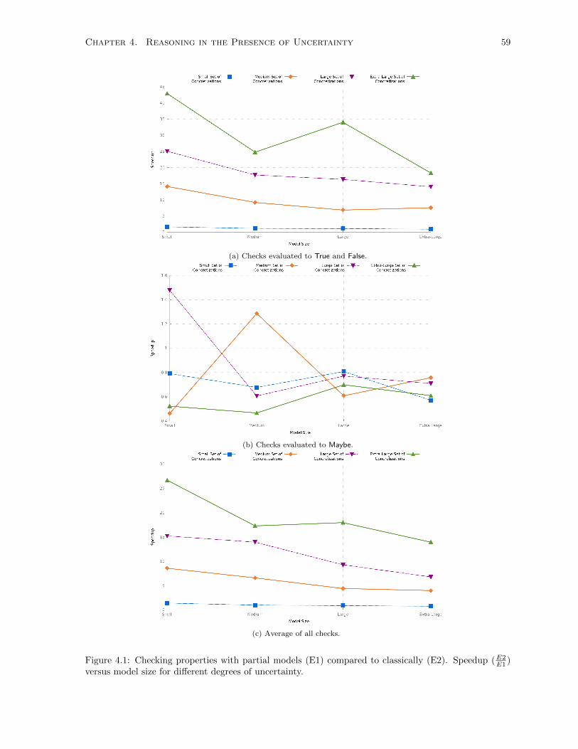
Chapter 4. Reasoning in the Presence of Uncertainty 59
(a) Checks evaluated to True and False.
(b) Checks evaluated to Maybe.
(c) Average of all checks.
Figure 4.1: Checking properties with partial models (E1) compared to classically (E2). Speedup (E2E1 )
versus model size for different degrees of uncertainty.

Chapter 4. Reasoning in the Presence of Uncertainty 60
4.3.6 Threats to validity
The most important threat to validity of our results stems from the use of experimental inputs that were
randomly generated. We attempted to mitigate this threat by using realistic parameters from previously
published example partial models, as described in Section 4.3.2.
Additionally, we conducted experiments with only a few input properties. We attempted to mitigate
this threat by selecting properties that were inspired from real well-formedness properties, published in
the literature (cf. Table 4.4).
Another threat to validity is induced by our choice to use a few exemplar values of the experimental
parameters in order to manage the combinatorial explosion of options. Generalizing our experimental
observations would require further, more fine-grained experimentation.
To compensate for these threats to validity, we additionally applied our technique to a large non-
trivial example based on fixing a bug of the UMLet editor [Auer et al., 2003]. The example, described in
Section 8.1, helped us triangulate our experimental results with experience from applying our technique
to a real world application. The size of the partial model that we extracted from UMLet, as well as
its set of concretizations, fell in the M category. The properties checked where “forall-exists”, similar
to Property 4 in Table 4.4 and returned True and Maybe. The observed speedups were even higher
than the experimental results presented in Section 4.3.5. This suggests that the experimental results
obtained from reasoning with randomly generated models may in fact constitute a lower bound, and
that reasoning with real models is even more efficient.
4.4 Related Work
In Section 3.5, we explained that partial models are an example of a common abstraction pattern where
multiple software artifacts are encoded in a single representation. We described three other formalisms
that follow the same pattern: metamodels, partial behavioural models, and software product lines. In this
section, we discuss work related to performing automated reasoning with such formalisms. Additionally,
we discuss related work from the field of database management.
Reasoning with metamodels. Metamodels are used to define the abstract syntax of modelling
languages, and thus a metamodel encodes the set of possible instance models that conform to it. In the
context of a multi-tier instantiation hierarchy, such as MOF [Object Management Group, 2006a], this
applies by extension to any model that can be instantiated. Reasoning about instances of metamodels is
typically done using constraint languages such as OCL [Object Management Group, 2006b]. Well known
systems that support verification using OCL include the Dresden OCL Toolkit [Demuth et al., 2009]
and USE [Gogolla et al., 2007]. Reasoning about models and metamodels is also done by leveraging
reasoning engines such as Alloy [Anastasakis et al., 2007] and Constraint Satisfaction Problem (CSP)
solvers [Cabot et al., 2007]. Partial model reasoning subsumes techniques for reasoning about models
and metamodels, since they can be used as part of its decision procedure instead of a SAT solver. For
example, in [Saadatpanah et al., 2012] we studied partial model reasoning using a variety of reasoning
engines, including Alloy and CSP.
Reasoning with partial behavioural models. We discussed the fundamental difference in semantics
between partial behavioural model verification and our approach in Section 4.1. In short, our approach

Chapter 4. Reasoning in the Presence of Uncertainty 61
is a language independent generalization of partial behavioural modelling. A corollary to language
independence is that the approach is only directly applicable for those analysis tasks that do not require
knowledge of the underlying semantics of the language. In order to apply to partial models, an analysis
technique that needs language semantics must first be “lifted” to accommodate partiality.
Lifting consists of adapting an existing decision procedure to make it uncertainty-aware, i.e., to give
it the capability to handle compact representations of sets of possibilities. A number of analyses have
been lifted to partial behavioural models: model-checking [Fischbein et al., 2012], pairwise compatibility
checking [Krka et al., 2014], and incremental refinement [Uchitel et al., 2013]. The concept of lifting is not
limited to reasoning. For example, in Chapter 5, we lift graph rewriting-based model transformations.
We are interested in developing a generic technique which can lift an arbitrary procedure, e.g., to make
it uncertainty-aware. This has been done, e.g., for reasoning with models of early requirements [Horkoff
et al., 2014].
In addition to property checking, the generation of artifacts similar to diagnostic cores, through
a process of property-driven refinement (see Chapter 6) has also been studied for partial behavioural
modelling [Uchitel et al., 2009], although with a method which is somewhat different from ours: properties
are synthesized as MTSs and then merged with the MTS of the system.
Reasoning with variability. There has been extensive research in adapting software engineering
techniques to make them variability-aware. Variability-aware techniques allow working at the level of
product lines rather than with explicit sets of individual products, and include techniques for model
checking [Classen et al., 2010], type checking [Kastner et al., 2012], testing [Kastner et al., 2012], graph
transformation [Salay et al., 2014], and others [Midtgaard et al., 2014; Thum et al., 2012]. Such tech-
niques are similar to our approach to reasoning with a set of possibilities at a high level of abstraction.
As discussed in Section 3.5, the main differences between partial model reasoning and these techniques
are (a) the different level of granularity in which sets are encoded, and (b) the different pragmatics and
context of usage between the two approaches.
Reasoning with databases. While models are used to create abstractions of software systems,
databases are used to abstract, store and manage data. The notion of uncertainty discussed in this
thesis is conceptually related to the management of incomplete databases, using possible worlds the-
ory [Abiteboul et al., 1987]. A well-known method for representing uncertainty in databases is the
tableau representation [Aho et al., 1979]. In fact, work on using tableaux to reason about multiple
repairs to inconsistency [Wijsen, 2005] was one of the initial inspirations for our work on partial models.
The diagnostic techniques presented in this chapter are also closely related to work in the database the-
ory, specifically in the context of data provenance [Buneman and Tan, 2007]. A typical data provenance
problem is query inversion, i.e., determining which tuples contributes to the output of a query [Buneman
et al., 2000].
4.5 Summary
In this chapter we discussed how partial models can be used to accomplish verification tasks in the
presence of uncertainty. We defined the meaning of partial model property checking and compared it
to partial behavioural model verification, which was the original inspiration for our approach. We ex-

Chapter 4. Reasoning in the Presence of Uncertainty 62
plained that because the partial models presented in this thesis have concretization-based semantics (i.e.,
are defined through structure-preserving refinement), we scoped our verification technique to checking
syntactic properties.
We gave a decision procedure for checking such properties and described the kinds of feedback that
can be generated in order to help developers perform diagnosis of their partial models. Specifically, we
described three kinds of diagnostic feedback: generating a counterexample concretization, generating an
example concretizations where the property holds, and generating a diagnostic core, i.e., a partial model
encoding the subset of concretizations that violate the property.
Finally, we performed an experimental evaluation of our verification approach. The goal of the exper-
iments was to assess the feasibility and scalability of property checking and counterexample generation.
We used randomly generated model inputs, on which we verified four properties from the literature
using a SAT solver. We found that partial model verification results in significant speedup compared to
classical verification (i.e., checking the property on each concretization separately). We also observed
that the speedup increases with greater degrees of uncertainty (i.e., larger sets of concretizations).
We describe how the results of property checking and diagnosis are used to guide the resolution
of uncertainty through property-driven refinement in Chapter 6. We also discuss how partial model
verification fits within the overall context of Model-Driven Engineering methodology in Chapter 7.

Chapter 5
Transforming Models Containing
Uncertainty
Model Driven Engineering (MDE) promises to accelerate and improve the quality of software develop-
ment: software is described using high-level models which are easy to reason with; these models are
then transformed into lower-level designs through a series of model transformations. Finally, low-level
designs are used for effective code generation. However, existing model transformation solutions do not
handle models with uncertainty. So when uncertainty is unresolved, the modeller should either delay the
application of transformations until more information becomes available, or make premature resolutions
in order to apply transformations, thus creating a risk that these resolutions are incorrect. In either
case, uncertainty diminishes the benefits of MDE.
In this chapter, we propose an approach that allows applying existing transformations to models
containing uncertainty. The essence of the approach involves automatically modifying – “lifting” –
transformations so they operate on partial models and correctly transform both the content of the
model and the uncertainty about it. As a result of our approach, transformations can be applied early in
the model development lifecycle, tolerating the uncertainty and allowing modellers to defer its resolution
until extra information is available. This eliminates the need to delay transformation application and
removes the pressure to potentially compromise model quality by resolving the uncertainty prematurely.
The rest of the chapter is organized as follows: In Section 5.1, we introduce the intuition of lifting
using a new running example, called SolvEx. SolvEx is smaller than the PtPP example introduced in
Chapter 1, thus allowing us to better illustrate lifted transformation application; it is also an example
of a structural, rather than a behavioural, modelling scenario, further illustrating the language indepen-
dence of partial modelling. In Section 5.2, we give the formal definition of lifting and describe lifted
transformation application. In Section 5.3, we describe the kinds of transformation properties preserved
by lifting. We discuss related work in Section 5.5 and conclude in Section 5.6.
The contents of this chapter have been published in [Famelis et al., 2013].
5.1 Intuition of Lifting
To motivate and illustrate the key points of our approach, we introduce a new example called SolvEx,
where a modeller is creating a UML class diagram for an automated reasoning engine. In SolvEx,
63

Chapter 5. Transforming Models Containing Uncertainty 64
(d)
Solver:Class
sn:nestedIn
SolverException:Class
m12
(e)
eo:owner
e:Attribute String:Class
ept:isPublicTrue:Bool
et:Type
Solver:Class
"effect":String
en:name
SolverException:Class
m13
eo:owner
e:Attribute String:Class
ept:isPublicTrue:Bool
et:Type
Solver:Classsn:nestedIn
"effect":String
en:name
SolverException:Class
m11
(c)
(b)
M1
eo:ownere:Attribute
String:Class
ept:isPublicTrue:Bool
et:Type
Solver:Class
sn:nestedIn
"effect":String
en:name
SolverException:Class
(sn ∧ e∧ eo∧ et∧ en∧ ept)∨(sn ∧¬e∧¬eo∧¬et∧¬en∧¬ept)∨(¬sn∧ e∧ eo∧ et∧ en∧ ept)
Φ =1
(a)
M1
SolverExceptionSolver
+ effect : String
x∨y
xy
sn
en
e
ept
et
eo
Figure 5.1: (a) partial model M1, showing points of uncertainty. (b) M1 as a typed graph (UML abstractsyntax). (c-e) Concretizations m11,m12,m13 of M1.
the modeller has decided that there should exist a class Solver which throws exceptions, objects of
type SolverException, whenever it reaches an error state. However, the modeller has yet to make
the following design decisions: (a) whether SolverException should be an inner class of Solver,
and (b) whether SolverException should have a String attribute called effect that would record an
estimation of the effect of the exception on the reasoning process. In addition, the modeller expects that
at least one of these features will be present in her model.
The resulting UML class diagram with uncertainty is encoded as a partial model M1 in Figure 5.1(a).
In this model, “⊕” is the UML symbol for a “nested class” and used here to indicate that SolverException
is an inner class of Solver. This model has two points of uncertainty – the relationship between the
classes Solver and SolverException (denoted by x) and the presence of the effect attribute in class
SolverException (denoted by y).
The modeller interacts with her tooling using the concrete UML syntax, i.e., the diagram in Fig-
ure 2.5(a). However, for the purpose of any automated task the model M1 is used in its abstract syntax.
In the rest of this chapter, we only consider models expressed in a simplified version of the UML ab-
stract syntax, defined by the metamodel in Figure 2.5(d). To better illustrate the details of each point
of uncertainty in M1, we show the model as a typed graph in Figure 5.1(b). In it, the node e and the
edges sn, eo, et, en, ept are annotated with Maybe and thus indicated using the star icon. We have
also included the type of each edge alongside the Maybe annotation. The May formula Φ1, also shown in
Figure 5.1(b), constrains the possible combinations of Maybe elements, defining the three concretizations
m11,m12,m13 shown in Figures 5.1(c-e), respectively.
Assume that the modeller notices that her model has an anti-pattern, namely, that the attribute
effect is public. She decides that, unless SolverException is an inner class, effect should be made
private for security reasons, and be accessed through a getter method. This can be accomplished by
performing the Encapsulate Variable refactoring [Casais, 1994]. A generic method for implementing this
refactoring using graph transformations was described by Mens et al. [Mens et al., 2005]. A simplified
version of this rule, called REV , is shown in Figure 5.2. The left-hand side (LHS) of the rule matches a
node a (and its associated edges such as ao:owner) that represents a public attribute. The right-hand
side (RHS) makes it private (by deleting the isPublic edge apt from a to True and adding a new
isPublic edge apf from a to False). It also creates a public getter operation ge and its associated

Chapter 5. Transforming Models Containing Uncertainty 65
Figure 5.2: Transformation rule REV for doing the Encapsulate Variable refactoring.
m23
(c)Solver:Class
sn:nestedIn
go:owner
ge:Operation
eo:owner
e:Attribute String:Class
TrueFalseepf:isPublic
et:Type gt:Type
gp:isPublic
SolverException:Class
"effect":String
en:name
"getEffect":String
gn:name
(b)
Solver:Class
sn:nestedIn
SolverException:Class
m22
eo:owner
e:Attribute String:Class
ept:isPublicTrue:Bool
et:Type
Solver:Classsn:nestedIn
"effect":String
en:name
SolverException:Class
m21
(a)
M2
(d)
( sn ∧ e∧ eo∧ et∧ en∧ ept∧ ¬epf∧¬ge∧¬go∧¬gt∧¬gn∧¬gp ) ∨( sn ∧ ¬e∧¬eo∧¬et∧¬en∧¬ept∧ ¬epf∧¬ge∧¬go∧¬gt∧¬gn∧¬gp )∨(¬sn ∧ e∧ eo∧ et∧ en∧¬ept∧ epf∧ ge∧ go∧ gt∧ gn∧ gp )
Φ =2
go:owner
ge:Operation
eo:owner
String:Class
True
Falseepf:isPublic
et:Type
gt:Type
gp:isPublic
SolverException:Class
Solver:Classsn:nestedIn
"effect":String
en:name
"getEffect":String
gn:name
ept:isPublic
e:Attributee
sn
eo
en
epf
ept
et
gtge
go
gp gn
Figure 5.3: (a-c) Classical models resulting from applying REV to the classical models in Figure 5.1(c-e).(d) The result of applying the lifted version REV to M1 directly: the partial model M2.
edges. In addition, the rule has two negative application conditions (NACs), i.e., conditions under which
the rule should not be applied. These are: NAC1, specifying the case when the class containing the
public attribute is an inner class, and NAC2, specifying the case when the class already has a getter.
Rule REV cannot be directly applied to the partial model M1 using the classical technique, described
in Section 2.3, because of uncertainty. Our goal is thus to create its “lifted” version, REV that can be
applied directly to M1. The intuition behind such a lifting is as follows: take the three concretizations,
m11, m12, m13, of M1; classically apply REV to each of them, resulting in models m21, 22, m23 in
Figure 5.3(a-c); represent the resulting models as a partial model M2 in Figure 5.3(d). That is, applying
the lifted rule to a partial model should be equivalent to a representation of the result of applying the
original rule to each of the concretizations of the partial model. So, applying the lifted version REV of
REV to M1 should produce the partial model M2 directly, without having to produce and transform
individual concretizations.
5.2 Lifting Algorithm
In this section, we describe the process of lifting a transformation rule to apply to partial models. We
focus on transformations based on graph rewriting [Ehrig et al., 2006], as described in Section 2.3.

Chapter 5. Transforming Models Containing Uncertainty 66
5.2.1 Specification of lifting
A classical rule R adapted to apply to partial models is called lifted and is denoted by R.
Partial models are intended to be exact representations of sets of models and lifted transformations
should preserve this. Therefore, applying a lifted transformation rule R to a partial model Min should be
equivalent to applying its classical version R to each of the concretizations of Min and building a partial
model from the result. We refer to this principle as the Correctness Criterion for lifting transformations
and define it formally below.
Definition 5.1. Let a rule R, a partial model Min with a set of concretizations [Min] = {m1in, . . . ,m
nin},
and the set U = {miout | ∀mi
in ∈ [Min] ·miin
R=⇒ mi
out} be given. R is a correct lifting of R iff for any
production MinR
=⇒ Mout, the set of concretizations of the resulting partial model Mout satisfies the
condition [Mout] = U .
In the SolvEx example, we aim to compute a lifted version REV of REV such that for the partial
models M1 and M2 in Figures 5.1(b) and 5.3(d), M1REV=⇒ M2.
In classical rule application during graph transformation (described in Section 2.3) it is sufficient to
find a graph match of the LHS of the rule and then check whether the NACs are applicable. However,
a partial model also has a propositional component, the May formula which constrains the possible
combinations of Maybe elements. Thus, doing the graphical match for the May graph is not sufficient
to guarantee correctness and needs to be augmented with manipulation of the May, to ensure that
the appropriate concretizations get transformed. We illustrate both parts of the transformation on
the SolvEx example in Section 5.2.2 and then generalize in Section 5.2.3. In Section 5.2.4 we prove
correctness of this approach.
5.2.2 Lifting example
We illustrate the transformation of the graph and the formula using the SolvEx example where the
rule REV in Figure 5.2 is applied to the partial model M1, shown in Figure 5.1(b), to produce M2 in
Figure 5.3(d). Figure 5.4 summarizes the application of this rule for the single existing matching site,
showing the diagrams and the truth tables of the May formulas Φ1 and Φ2 of M1 and M2, respectively.
Each column of the truth tables is a Maybe element. Each row corresponds to an allowable configuration
of Maybe elements, denoted by 1, and thus defines a concretization. The truth tables also show which
Maybe elements are matched by each of the rule’s parts (the parts of REV are shown in Figure 2.6). For
example, the edges eo and ept are both matched by the rule’s LHS, where eo is found in the match
C of the Cr part of the rule, and ept in D match of Dr. Our objective is to construct the lifted
transformation REV that produces M2 when applied to M1. We begin by constructing the graphical
part of REV first, followed by the propositional part.
Graphical part Consider applying REV to M1 by directly applying it to Mb, M1’s base graph. Clearly,
this approach does not produce the correct outcome. First, NAC1 matches in Mb and thus the rule does
not apply at all! Yet, there exists a concretization of M1, m13, for which neither of REV ’s NACs match
and thus REV should be applicable. We therefore expect it to be applicable to M1 as well. Second, the
RHS of the rule does not specify which elements in the output model should become Maybe, whereas
M2 clearly has them.
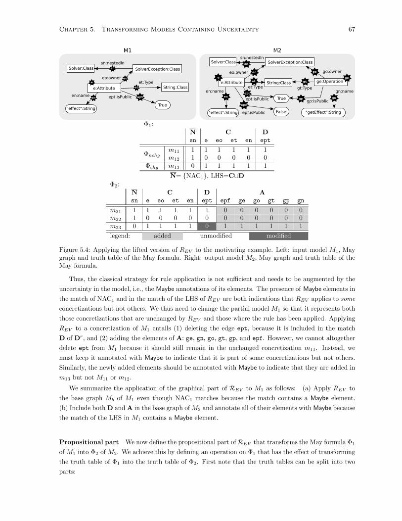
Chapter 5. Transforming Models Containing Uncertainty 67
go:owner
ge:Operation
eo:owner
e:Attribute String:Class
True
Falseepf:isPublic
et:Type gt:Type
gp:isPublic
SolverException:ClassSolver:Classsn:nestedIn
"effect":String
en:name
"getEffect":String
gn:name
ept:isPublic
M1 M2
e
sn
eo
en
epf
ept
et gtge
go
gp gn
Solver:Classsn:nestedIn
SolverException:Class
eo:owner
e:Attribute String:Class
True
ept:isPublic
et:Type
"effect":String
en:name
sn
en
e
ept
et
eo
Φ1:N C Dsn e eo et en ept
Φnchgm11 1 1 1 1 1 1m12 1 0 0 0 0 0
Φchg m13 0 1 1 1 1 1
N= {NAC1}, LHS=C∪D
Φ2:N C D Asn e eo et en ept epf ge go gt gp gn
m21 1 1 1 1 1 1 0 0 0 0 0 0m22 1 0 0 0 0 0 0 0 0 0 0 0m23 0 1 1 1 1 0 1 1 1 1 1 1
legend: added unmodified modified
Figure 5.4: Applying the lifted version of REV to the motivating example. Left: input model M1, Maygraph and truth table of the May formula. Right: output model M2, May graph and truth table of theMay formula.
Thus, the classical strategy for rule application is not sufficient and needs to be augmented by the
uncertainty in the model, i.e., the Maybe annotations of its elements. The presence of Maybe elements in
the match of NAC1 and in the match of the LHS of REV are both indications that REV applies to some
concretizations but not others. We thus need to change the partial model M1 so that it represents both
those concretizations that are unchanged by REV and those where the rule has been applied. Applying
REV to a concretization of M1 entails (1) deleting the edge ept, because it is included in the match
D of Dr, and (2) adding the elements of A: ge, gn, go, gt, gp, and epf. However, we cannot altogether
delete ept from M1 because it should still remain in the unchanged concretization m11. Instead, we
must keep it annotated with Maybe to indicate that it is part of some concretizations but not others.
Similarly, the newly added elements should be annotated with Maybe to indicate that they are added in
m13 but not M11 or m12.
We summarize the application of the graphical part of REV to M1 as follows: (a) Apply REV to
the base graph Mb of M1 even though NAC1 matches because the match contains a Maybe element.
(b) Include both D and A in the base graph of M2 and annotate all of their elements with Maybe because
the match of the LHS in M1 contains a Maybe element.
Propositional part We now define the propositional part ofREV that transforms the May formula Φ1
of M1 into Φ2 of M2. We achieve this by defining an operation on Φ1 that has the effect of transforming
the truth table of Φ1 into the truth table of Φ2. First note that the truth tables can be split into two
parts:

Chapter 5. Transforming Models Containing Uncertainty 68
(a) The concretizations where REV does not apply (i.e., m11 and m12). The corresponding rows m21
and m22 in Φ2 remain unchanged, and the variables in A are set to False (denoted by 0) to indicate
that Ar is not added. We denote the formula representing the unchanged part by Φnchg.
(b) The concretizations where REV does apply (i.e., m13). The corresponding row m23 has the variables
of D set to 0 to indicate that Dr is deleted and the variables of A set to 1 to indicate that Ar is
added. We denote the formula representing the changed part by Φchg.
Thus, Φ2 = Φnchg ∨ Φchg.
To obtain the unchanged part, we begin by specifying a condition, over elements of M1, under which
the rule REV applies, i.e., when its NAC Nr does not match in Mb and both Cr and Dr do match:
Φapply = ¬φandN ∧ φandC ∧ φandD . Let φandX where X ∈ {N,C,D} denote the conjunction of all variables in
X that represent elements that are Maybe. Restricting Φ1 to those concretizations of M1 where REV
does not apply (¬Φapply) and forcing the variables of A to become False produces the unchanged part:
Φnchg = (Φ1 ∧ ¬Φapply) ∧ ¬φorA , where φorA indicates the disjunction of all variables in A that represent
elements that are Maybe.
For the changed part Φchg, we restrict Φ1 to those concretizations of M1 where REV does apply and
force the variables of D to become False and those of A to become True: Φchg = (Φ1 ∧ Φapply)|∃D ∧¬φorD ∧φandA . Here, (Φ1∧Φapply)|∃D indicates existential quantification of all variables in D that occur in
formula Φ1∧Φapply. In our example, D = {ept}, so it becomes (Φ1∧Φapply)|ept=T ∨(Φ1∧Φapply)|ept=F .
That is, we eliminate each variable in D from Φ1 ∧ Φapply by taking the disjunction of the cases where
it is set to False and to True. Quantifying out variables in D is done before forcing them to become
False (using ¬φorD ) because we are changing the values of existing variables (the variables of D already
occur in Φapply) and not just setting the value for new variables as we are for A. Otherwise, we get an
inconsistency because Φapply ⇒ φandD by definition.
Substituting the variables from the example and simplifying gives:
Φnchg =(sn ∧ e ∧ eo ∧ et ∧ en ∧ ept ∧ ¬epf ∧ ¬ge ∧ ¬go ∧ ¬gt ∧ ¬gt ∧ ¬gp ∧ ¬gn)∨
(sn ∧ ¬e ∧ ¬eo ∧ ¬et ∧ ¬en ∧ ¬ept ∧ ¬epf ∧ ¬ge ∧ ¬go ∧ ¬gt ∧ ¬gt ∧ ¬gp ∧ ¬gn)
Φchg =(¬sn ∧ e ∧ eo ∧ et ∧ en ∧ ¬ept ∧ epf ∧ ge ∧ go ∧ gt ∧ gt ∧ gp ∧ gn)
The resulting formula Φ2 = Φnchg ∨ Φchg is the same as the May formula in Figure 5.3(d) and has the
same truth table as the one shown in Figure 5.4.
5.2.3 General case
We can generalize the above process to an arbitrary rule R and define how the graphical part of its lifted
version R is applied to a partial model M to produce a partial model M ′. As with the SolvEx example,
we define this in terms of applying R to the base graph of M and then making modifications. Following
Definition 2.7, the matching site for R is a matching site for R in the base graph of M .
Definition 5.2 (Lifted rule applicability conditions). Given a partial model M with a May formula ΦM ,
a transformation rule R = 〈{NAC},LHS,RHS〉, and a matching site K = 〈N,C,D〉, the lifted rule R is
applicable at K iff the following conditions hold:
1. For all N ∈ N, N contains a Maybe element
2. ΦM ∧ Φapply is satisfiable, where Φapply = ¬∨{φN |N ∈N} ∧ φandC ∧ φandD .

Chapter 5. Transforming Models Containing Uncertainty 69
In this definition, Condition 1 ensures that there is no NAC match without Maybe elements; otherwise
the NAC match would necessarily occur in every concretization and so R would not apply to any
concretization of M . Condition 2 uses the constraints in the May formula to ensure that at this matching
site, the rule R matches in at least one concretization of M . Specifically, this checks that there exists a
concretization in which all f the Maybe elements of C and D are True and not all of the Maybe elements
in any NAC match are set to True.
We now give the general definition of a rule application for a lifted rule.
Definition 5.3 (Lifted rule application). Assume a partial model M with a May formula ΦM , a trans-
formation rule R = 〈{NAC},LHS,RHS〉 and matching site K = 〈N, C, D〉 in M for which the rule
applicability conditions are satisfied. We define the lifted application of R as the following process to
apply the lifted rule R to M to produce a partial model M ′:
1. if K contains no Maybe elements, apply R in the classical way to produce the base graph of M ′
and set φM ′ = φM .
2. otherwise,
(a) set M ′ = M ;
(b) add the elements A of the Ar part of the RHS to M ′;
(c) annotate all elements of A and D with Maybe;
(d) set ΦM ′ = [(ΦM ∧ ¬Φapply) ∧ ¬φorA ] ∨ [(ΦM ∧ Φapply)|∃D ∧ ¬φorD ∧ φandA ].
In the following we refer to lifted application simply as application.
In this definition, Case 1 captures the situation when there are no Maybe elements at the matching
site and so the rule can be applied in the classical way and the partial model is unaffected. Case 2
captures the situation when there are Maybe elements in parts of the matching site so that R may apply
in some concretizations but not in others. This case mirrors the discussion of REV in Section 5.2.2. In
particular, in the graphical part, Dr is not deleted (step a) but Ar is still added (step b) and all of the
elements in A and D are set to Maybe (step c). The propositional part (step d) is the same as for the
REV example except that Φnchg and Φchg are inlined and the more general case of N is used in Φapply
(from Definition 5.2) to account for multiple NAC matches that could exist in the base graph of M .
As with a classical rule system, lifted rules continue to be applied until no rule is applicable. Note
that the resulting model M ′ may not necessarily be in GRF after every rule application. That is, M ′ can
contain redundant Maybe elements. If M ′ is intended for human consumption (as opposed to automated
reasoning) then the additional step of putting it into GRF is advisable. However, this step is optional
since it does not affect the set of concretizations that the partial model represents.
5.2.4 Correctness
We now show that lifting described by Definitions 5.2 and 5.3 satisfies the correctness condition in
Definition 5.1. Specifically, we prove the following theorem:
Theorem 5.1. Lifted application of a rule R produces a correct lifting of R.
In other words, if the lifted version R of a rule R is applied to a partial model M to produce a partial
model M ′, then the concretizations of M ′ must be exactly the set obtained by applying the classical rule
R to each concretization of M . We focus our argument on a specific matching site since by transitivity, if
the rule is correct when applied to each site, then the application to any sequence of sites is also correct.

Chapter 5. Transforming Models Containing Uncertainty 70
We begin by checking correctness of the applicability condition (see Definition 5.2) of the lifted rule
R: whenever R is applicable for some concretization of M at K, then R is also applicable, i.e., R it
does not miss any sites where a concretization can be affected by R. By Condition 1 of Definition 5.2,
if there is a NAC in N that has no Maybe elements then R does not apply at K. But a NAC without
Maybe in the base graph of M means that this NAC appears in every concretization of M and thus the
classical rule R does not apply to any concretization either and thus applying the lifted rule does not
miss any classical rule applications.
Condition 2 says that ΦM ∧Φapply must be satisfiable for R to apply, which happens iff there exists
a concretization of M where Cr and Dr are present and no NAC in N is present – exactly the classical
applicability condition in Definition 2.8. If this condition does not hold, there are no classical rule
applications in any concretization; therefore, the lifted rule applicability condition is correct.
We now argue that the lifted rule application in Definition 5.3 is correct. To do this, we show that if
R satisfies the applicability conditions, then applying R at a site K has the same effect as applying R
at K in each concretization. Case 1 says that when K contains no Maybe elements, we apply the rule
classically to the base graph of M . Without Maybe elements, K occurs in every concretization of M and
so the classical application of R in every concretization would be identical to applying R.
Case 2 applies when K has some Maybe elements. In this case, the concretizations are split into
those where R does not apply and those where it does. We then aim to show that the steps (a-d) for
constructing the graphical and propositional effect of applying R are “correct by construction”. We do
not repeat this argument, described in Section 5.2.2, here, for brevity. Thus, we conclude that the lifted
rule application is also correct. Since both the applicability condition and the effect of application are
correct, we conclude that R satisfies the specification of correct lifting in Definition 5.1.
5.3 Properties of Lifted Transformations
In this section, we show that lifting preserves the confluence and termination of graph rewriting systems
(GRSs) (see Section 2.3.2), i.e., that if a GRS has some these properties, its version containing lifted
transformations does as well.
5.3.1 Termination
We need to prove the following theorem:
Theorem 5.2 (Preservation of termination). Assume a partial model M , a set S of graph rewriting
rules {R1, . . . , Rn} and the set S = {R1, . . . ,Rn} containing lifted version of the rules in S. If for
every concretization mi ∈ [M ] the GRS Gi = 〈S,mi〉 is terminating, then the GRS G = 〈S,M〉 is also
terminating.
Without loss of generality, we restrict ourselves to a rule set containing a single classical rule R which
we assume is terminating. Since R is correct according to Definition 5.1, repeatedly applying it to a
partial model M has the same effect as repeatedly applying R to each concretization of M . Since R is
terminating for every concretization in M , it eventually is no longer applicable to any of them. At this
point, Φapply, which encodes classical applicability, is False and thus ΦM ∧Φapply is not satisfiable, and,
by Condition 2 of Definition 5.2, R does not apply. Thus, when the application of R terminates, the

Chapter 5. Transforming Models Containing Uncertainty 71
application of R terminates as well. Therefore, if R is terminating for each concretization, so is R for
the partial model encoding them.
5.3.2 Confluence
We argue that if a set of classical rules is confluent then the corresponding set of lifted rules is also
confluent “up to an equivalence”, that is, when the process terminates, the resulting partial model has
the same set of concretizations, regardless of the order in which the rules have been applied. We therefore
need to prove the following theorem:
Theorem 5.3 (Preservation of confluence). Assume a partial model M , a set S of graph rewriting rules
{R1, . . . ,Rn} and the set S = {R1, . . . ,Rn} containing lifted version of the rules in S. If for every
concretization mi ∈ [M ] the GRS Gi = 〈S,mi〉 is confluent and terminating, then the GRS G = 〈S,M〉is also confluent.
Since for every concretization mi ∈ [M ] the GRS Gi = 〈S,mi〉 is confluent and terminating, for each
one there exists an “ultimate” transformed version hi such that miS∗=⇒ hi. Since R is correct according
to Definition 5.1, repeatedly applying lifted rules to a partial model M has the same effect as repeatedly
applying the corresponding classical rules to each concretization of M . In other words there is a partial
model H such that MS∗=⇒ H, where [H] = {hi|mi
S∗=⇒ hi,mi ∈ [M ]}. Thus, the lifted rule set is
confluent “up to an equivalence”.
5.4 Evaluation
We applied our lifting approach to the problem of mapping simple UML class diagrams to relational
database schemas. This problem is called “Object-Relational Mapping” (ORM) and is often used as
a benchmark for model transformations [Bezivin et al., 2006]. Our aim was to gather evidence about
how the lifting approach scales as uncertainty increases. We thus measured the runtime of performing
ORM with lifted rules while increasing levels of uncertainty and compared it with the baseline runtime
of performing ORM for a classical model. The ORM transformation we used was published in [Varro
et al., 2006] and consists of 5 layered transformation rules that, given a class diagram, create a relational
schema and traceability links. The rules and the source and target metamodels are shown in Appendix C.
We used the class diagram specification of the Ecore metamodel [Steinberg et al., 2009] as input to the
ORM rules. Serializing Ecore models in a database is an important technical problem that has resulted
in the establishment of two Eclipse projects, CDO [Eclipse, accessed 2013-03-16a] and Teneo [Eclipse,
accessed 2013-03-16b], both of which implement ORM for Ecore. We manually flattened the Ecore
metamodel and adapted it to the type graph used by the ORM rules in [Varro et al., 2006]. The resulting
model consisted of 65 model elements: 17 classes, 17 associations, 6 generalization links and 25 attributes.
Starting with a partial model with a single concretization (no uncertainty), we gradually increased the
degree of uncertainty by adding more concretizations, by a step of roughly 50, thus creating models
with 1, 24, 48, 108, 144, 192, and 256 concretizations. To accomplish that we incrementally injected
points of uncertainty, annotating elements with Maybe and creating the corresponding May formulas.
The most uncertain case (256 concretizations) contained 8 points of uncertainty, expressed across a total
of 14 Maybe elements. We show the partial Ecore metamodel with the largest set of concretizations in
Appendix C.

Chapter 5. Transforming Models Containing Uncertainty 72
Table 5.1: Results of applying the ORM rules to the Ecore metamodel.Number of concretizations: 1 24 48 108 144 192 256
Number of Maybe elements: 0 5 6 8 10 12 14
Time (sec): 32.6 32.8 32.7 32.9 32.6 33.0 48.4Size of May formula (KiB): 0 27.9 14.0 1,080.9 1,153.4 19,361.9 320,570.7
We implemented the lifting of the ORM rules using Henshin [Arendt et al., 2010]. For the satisfiability
check required in Definition 5.2, we used the Z3 SMT solver [De Moura and Bjørner, 2011]. We used
MMINT [Di Sandro et al., 2015] as the integration platform. We executed the case study on a computer
with Intel Core i7-2600 3.40GHz×4 cores (8 logical) and 8GB RAM, running Ubuntu-64 12.10. We
applied the set of lifted rules to each input partial model and recorded the total runtime and the size of
the resulting May formula. Our observations are shown in Table 5.1.
The results show that the total runtime remains almost constant at roughly 32.8 seconds, except for
the largest category where it increases to 48.4 seconds. On the other hand, we see a dramatic increase in
the size of the May formula, from 27.9 KB for the smallest category, to approximately 320.6 MB for the
largest. This exponential growth in size is expected, given that the output May formula is constructed
using existential quantification ( Definition 5.3). Overall, the results suggest that lifting scales reasonably
with respect to time, whereas the increasing size of the May formula may be a problem. However, we
note that our implementation did not attempt to incorporate any formula simplification heuristics, and
therefore there is room for optimization.
5.5 Related Work
Partial models encode a set of classical models, and lifted rules are rules that can transform entire sets
of models simultaneously. In the following, we discuss work related to transformations that apply to
modeling formalisms that represent sets of models.
Different variants of feature models have been proposed in the literature to encode a set of possible
configurations of a software product line [Schobbens et al., 2006]. Transformations of feature models,
i.e., the creation of a feature model representing a subset of the original, have been studied in [Czarnecki
et al., 2004] under the name of feature model specialization. This process is described as a series of
operations such as “feature cloning” and “reference unfolding” and resembles the uncertainty-reducing
refinement described in Chapter 6. Graph transformations have also been applied to feature models,
e.g., in [Segura et al., 2008], they are used to refactor product lines via feature model merging.
Transformations that apply to metamodel definitions also transform sets of models, i.e., the set of
possible instances of the metamodel. The Object-to-Relational Mapping transformation [Varro et al.,
2006] in Section 5.4 is one such example. Similarly, special purpose transformation languages have been
built to transform ontologies, such as a rule based language based on xOWL [Wouters and Gervais,
2012].
The main difference between these transformations and the lifting approach presented here is that
they are tailored to specific tasks, whereas lifting applies to arbitrary transformation rules. Moreover,
these techniques only indirectly affect the classical models (e.g., variants or instances) represented by the
abstraction formalism. On the other hand, lifted transformations match and transform the alternatives
directly, via the propositional part of the lifted rules.

Chapter 5. Transforming Models Containing Uncertainty 73
We have adapted the lifting of graph-based transformations so that it can be applied to annotative
software product lines [Salay et al., 2014]. An annotative product line consists of a domain model,
a feature model, and a feature mapping, that annotates elements of the domain model with presence
conditions, i.e., propositional expressions over features (see also Section 3.5.3) Applying lifted transfor-
mations to product lines involves transforming the domain model and then manipulating the presence
conditions such that the resulting product line satisfies a correctness criterion very similar to the one
in Definition 5.1. Lifting transformations for product lines is more efficient than for partial models: (a)
propositional manipulations deal only with the presence conditions of elements at the transformation
application site, and (b) presence conditions tend to be simpler expressions than a full blown May for-
mula. We have taken advantage of this fact to create support for transforming industrial-grade software
product lines [Famelis et al., 2015b] by lifting DSLTrans [Selim et al., 2014; Lucio et al., 2010], a model
transformation language that specializes in helping developers create provably correct transformations.
5.6 Summary
In this chapter, we have shown how to apply graph-based model transformations to partial models. We
have introduced the concept of lifting: applying a transformation to a partial model should produce a
new partial model which should be the same as if we had transformed each concretization of the input
partial model separately and then merged them back. This means that existing transformations remain
unchanged: it is the semantics of the transformation engine that changes. Specifically, we defined a
three-step process for applying lifted transformations: given a matching site, first we use a SAT solver to
determine whether the rule is applicable to at least one concretization at that site; then we transform the
graphical part of the partial model; finally we transform the May formula to ensure that the correctness
of lifting is respected. We showed that our process preserves lifting correctness, as well as confluence
and termination.
We have applied our approach to the Object-Relational Mapping, a common benchmark for model
transformation techniques. Specifically, we systematically injected uncertainty to the Ecore metamodel,
resulting in partial models with increasing degrees of uncerainty. The benchmark indicates that there is
a trade-off between low runtime and the growth of the May formula.
We discuss how the lifting of transformations fits within the overall context of Model-Driven Engi-
neering methodology in Chapter 7.

Chapter 6
Removing and Resolving
Uncertainty
If developers lack information required to select among multiple possibilities, they can use partial models
to explicate their uncertainty within their software artifacts. As discussed in Section 3.1, an important
characteristic of partial models is that the size of the set of concretizations reflects the modeller’s degree of
uncertainty. A larger set of concretizations corresponds to a higher degree of uncertainty. Using partial
model reasoning and lifted transformations developers can defer premature resolution of uncertainty
while still being able to perform engineering tasks. This means that, while decisions are deferred, the
size of the set of concretizations remains unchanged (cf. the definition of lifting in Section 5.2). In this
chapter, we discuss how developers can resolve uncertainty once deferral is no longer necessary.
The topic of decision making in the presence of uncertainty is extensively studied in diverse fields
of research such as Decision Theory, Design Space Exploration, and others. We limit our focus to the
question of leveraging partial models to support the resolution of uncertainty. In other words, our
aim here is not to help developers make decisions. Rather, once decisions are made (using whatever
rationale), our goal is to correctly incorporate this new information to partial models.
We formally introduced refinement as a relationship between partial models in Definition 3.5: “Given
two partial models M1 and M2, we say that M2 refines M1 (or that M1 is more abstract than M2),
denoted M2 � M1, iff C(M2) ⊆ C(M1), and M2 is consistent.” In this chapter, we operationalize this
definition, and describe refinement as an engineering task that reduces the number of concretizations of
a partial model, either manually or automatically.
The rest of this chapter is organized as follows: In Section 6.1, we describe how to refine partial
models, based on the formal semantics of refinement introduced in Section 3.1. Specifically, we introduce
two ways of accomplishing this: manual decision making and property-driven refinement. In Section 6.2,
we study experimentally the efficiency and sensitivity of the property-driven refinement technique. In
Section 6.3, we discuss related work, and we conclude in Section 6.4. Proofs of theorems are found in
Appendix A.2.
The contents of this chapter, with the exception of Section 6.1.1, have been published in [Famelis
et al., 2012] and expanded in the manuscript [Famelis et al., 2015c], currently under review.
74

Chapter 6. Removing and Resolving Uncertainty 75
6.1 Uncertainty-Removing Refinement
In this section, we discuss how a modeller can incorporate new information into a partial model, thus
resolving uncertainty. Since the degree of uncertainty in a partial model is determined by the size of
its set of concretizations, reducing uncertainty is tantamount to reducing the size of this set. If this is
done incrementally we refer to this process as removal of uncertainty. Alternatively, it can be done at
once by reducing the set of concretizations to a single solution, in which case we say that uncertainty
is resolved. The theory of partial models allows accomplishing both tasks in a well defined, formal
process of refinement [Salay et al., 2012c]. As discussed in Section 4.1.1, partial model refinement is
structure-preserving as opposed to trace-preserving.
In the following, we describe the pragmatics of refinement, describing two ways to accomplish it. The
first way, which we call “manual decision making”, involves point-wise modifications to the annotations of
partial model elements. The second, which we call “property-driven refinement”, entails using properties
to constrain the set of concretizations. Manual decision making and property-driven refinement are
analogous to the Graphical and Propositional Reduced Forms (GRF and PRF), introduced in Section 3.3.
On the one hand, like GRF, manual decision making puts the focus on working with the diagrammatic
aspect of parital models. On the other hand, like PRF, property-driven refinement puts the focus on
working with their logical aspect1.
6.1.1 Manual decision making
A partial model can be refined by manually changing the annotations of its atoms and the May formula
to decrease the level of uncertainty. These changes reflect the modeller’s judgement about how the newly
acquired information should be represented in the model.
Performing manual decision-making is accomplished by using two atomic partial model operators,
named Keep and Drop.
Invoking Keep for a partial model element amounts to making a decision that the element should be
present in the model.
Definition 6.1 (Keep). Given a partial model M1 = 〈G1, ann1, φ1〉 and an element e ∈ G1 such that
ann1(e) = Maybe, the operator Keep generates a new partial model M2 = 〈G2, ann2, φ2〉 such that:
• G2 = G1;
• ann2(e) = True and ∀a ∈ G2, a 6= e, ann2(a) = ann1(a), i.e., change the annotation of e to True;
• φ2 = φ1[True/atomToProposition(e)], i.e., replace e’s encoding by True
The function atomToProposition() is defined in Section 2.1.2.
Conversely, invoking Drop for a partial model element amounts to deciding that it should not be part
of the model. To ensure that Drop always results in a well-formed diagram, we define two variants, one
for elements that are edges and one for vertices.
Definition 6.2 (DropEdge). Given a partial model M1 = 〈G1, ann1, φ1〉 and an edge element e ∈ G1
such that ann1(e) = Maybe, the operator DropEdge generates a new partial model M2 = 〈G2, ann2, φ2〉such that:
1We do not imply that either refinement method is better suited to a particular reduced form.
Chapter 6. Removing and Resolving Uncertainty 76
• e /∈ G2 and ∀a 6= e : a ∈ G2 ⇔ a ∈ G1, i.e., delete e;
• ∀a ∈ G2, ann2(a) = ann1(a);
• φ2 = φ1[False/atomToProposition(e)], i.e., replace e’s encoding by False
Definition 6.3 (DropVertex). Given a partial model M1 = 〈G1, ann1, φ1〉 and a vertex element e ∈G1 such that ann1(e) = Maybe, and there are no incoming or outgoing transitions to e, the operator
DropVertex generates a new partial model M2 = 〈G2, ann2, φ2〉 such that:
• e /∈ G2 and ∀a 6= e : a ∈ G2 ⇔ a ∈ G1, i.e., delete e;
• ∀a ∈ G2, ann2(a) = ann1(a);
• φ2 = φ1[False/atomToProposition(e)], i.e., replace e’s encoding by False
DropVertex has a strong requirement that only Maybe vertices without incoming or outgoing edges
can be removed from the model. This has two implications: First, Maybe edges connected to the vertex
should be removed first, using DropEdge. Second, if a vertex is connected with edges annotated with True,
then it cannot be removed from the model via refinement. This is because annotating an edge with True
indicates that the modeller is certain that it should be in the model; thus, removing it to satisfy graph
well-formedness would be counter-intuitive. Instead, the strict requirement ensures that this apparent
contradiction is scrutinized, potentially exposing faults in the original modelling of uncertainty.
Keep, DropEdge and DropVertex are atomic (in the sense that they affect one element at a time)
refining operators:
Theorem 6.1. Given a partial model M , and an element e ∈M , Keep(M,e) �M and DropEdge(M,e)
�M if e is an edge or DropVertex(M,e) �M if it is a vertex.
Resolving uncertainty about a decision point is therefore a matter of repeatedly applying Keep,
DropEdge and DropVertex for all Maybe elements that are relevant to it. For example, the partial
model Mt in Figure 1.6 can be refined to the one in Figure 1.7 through a series of invocations of the
operators, such as the series: Keep(Mt, At); Keep(Mt, H2); Keep(Mt, Et); Keep(Mt, Fs); Keep(Mt, H4);
Keep(Mt, Ga); Keep(Mt, Gt); DropEdge(Mt, Aa); DropEdge(Mt, Ba); DropEdge(Mt, Bt); DropEdge(Mt, Da);
DropEdge(Mt, Dt); DropEdge(Mt, Ea); DropVertex(Mt, H1). No action is taken for the Maybe elements
Ca, Ct, H3, H5. The May formula shown in Figure 1.7 has been simplified.
We note that this method of making decisions also implies that: (a) no new elements can be added to
the partial model, (b) elements that are annotated with True cannot be deleted, and (c) the annotations
of True elements cannot be changed. Applying one of the two operators to each Maybe element of the
partial model, obviously results in a concretization (cf. Definition 3.2).
Decision-making can be automated, by creating batch uncertainty-reducing transformations (URTs).
A simple example of an URT would be one that deletes all Maybe atoms. URTs are different from the
lifted transformations discussed in Chapter 5. Lifting aims to apply to partial models transformations
written for non-partial models (such as refactoring, translations, etc.) and aims at preserving rather
than reducing the set of concretizations. The main concern with using URTs is ensuring that they are
indeed refining. We have studied this for URTs based on graph-rewriting, applied to a subclass of partial
models that do not have May formulas in [Salay et al., 2015]. For such partial models, proving that a
URT is refining requires proving that the rule’s right hand side (RHS) is a refinement of its left hand
side (LHS).

Chapter 6. Removing and Resolving Uncertainty 77
ALGORITHM 5: Computing all concretizations of a given model that satisfy a given property.
Input: A partial model M = 〈GM , annM , φM 〉 of type T and a grounded property formula φpOutput: A partial model Mp �M , such that ∀m ∈ C(Mp) ·m |= φp
1 Generate M PRF from M using Algorithm 2;
2 Gr := GMPRF ;
3 foreach atom a ∈ GMPRF do annr(a) = Maybe;
4 φr := φMPRF ∧ φp;
5 Mr := 〈Gr, annr, φr〉;6 Generate Mp := GRF of Mr using Algorithm 1;7 return Mp;
6.1.2 Property-driven refinement
Property-driven refinement provides a means to resolve uncertainty in a declarative way. Instead of
manually making decisions about each Maybe element separately, the modeller specifies her refinement
rationale using a property. Using the reasoning technique described in Chapter 4, the modeller is able
to determine whether the property holds for all, some or none of the partial model’s concretizations.
The partial model property checking decision procedure Section 4.1.2 returns True, Maybe, and False
respectively. If the result of property checking is True or False, the model already satisfies or violates the
property regardless of how uncertainty is resolved. This may signify that the specified property is not a
good guide for uncertainty resolution, that there is nothing the developer needs to do, or that there is
nothing the developer can do without first changing the partial model. In this section, we focus on the
third possibility, i.e., when the result of property checking is Maybe.
If the result of property checking is Maybe, the developer can use the property to constrain the partial
model so that it ends up with a subset of the originial set of concretizations. Effectively, the property
can be used as a “filter” to remove unwanted possibilities from the partial model and ensure that all of
its concretizations satisfy the property. In the PtPP example, assume that the team decides that the
property P4 (“ Users can always cancel any operation, i.e., every non-idle state has a transition to Idle
on cancel”) should be satisfied by the model Mp2p shown in Figure 1.3. The team should therefore be
able to restrict their working set of alternatives to those that satisfy it, i.e., those in Figure 1.4(a-d).
Assume that the result of verification of an important property p on a partial model M of type T
is Maybe. The subset of concretizations of M that satisfy p is exactly characterized by the formula
F+(T,M, p) defined in Section 4.1.2. We use this formula to construct the partial model Mp using
Algorithm 5. In particular, first we put M into PRF (Line 1). Then, we construct an intermediate
partial model Mr (Lines 2-5) directly in PRF, by copying over the graph of M , annotating all atoms
with Maybe and setting its May formula to φMPRF ∧ φp. This way, we add the property as part of the
May formula and thus restrict the set of concretizations to only those satisfying the property. Finally,
we put Mr into GRF, using Algorithm 1, and return it (Lines 6-7).
Since the conversion of M to PRF and the creation of the intermediate model Mr are linear in the
number of atoms of the input model, the complexity of the algorithm is that of the GRF conversion,
i.e., NP-hard.
Using Algorithm 5, we can refine a partial model using a grounded property as a filter for its con-
cretizations:
Theorem 6.2. Let model Mp be a result of running Algorithm 5 on a model M . Then, Mp � M and

Chapter 6. Removing and Resolving Uncertainty 78
∀m ∈ C(Mp) ·m |= φp.
In the PtPP example, consider the property P5=¬ P2, where P2 is the property “no two transitions
have the same source and target”. The concretizations of Mp2p that satisfy P5 are those that satisfy the
formula F+(SM, Mp2p, P5), i.e., those in Figure 1.4(c, d). The partial model MP5p2p that represents them
is shown in Figure 3.4(a). To construct it, we first put the model Mp2p in Figure 1.3 in PRF. We then
conjunct its May formula with φP5. After removing all superfluous atoms and simplifying, we end up
with the model in Figure 3.4(b). Creating its GRF equivalent results in the model in Figure 3.4(a).
Note that in the example above, since P5=¬P2, we used property-driven refinement to create a
partial model that only has concretizations that violate the property P2. As discussed in Section 4.2.3,
this is a form of feedback, called diagnostic core, that can be generated after property checking to help
users understand the commonalities between concretizations that violate a property.
6.2 Experimental Study of Property-driven Refinement
In this section, we present an experimental evaluation of property-driven refinement. Contrary to the
experimentation presented in Section 4.3, it is not meaningful to compare property-driven refinement
with some “classical” approach. Specifically, while it is possible to compute the set of all possible
concretizations that satisfy a property without using partial models, doing so would not have the same
effect as performing property-driven refinement. The reason is that property-driven refinement creates
a GRF partial model which is a visual representation of the set.
This allows interacting with this set in ways that are not possible or meaningful with an enumerated
set of classical models. For example, in PtPP, when reasoning with the property P2 (“no two transitions
have the same source and target”), generating a diagnostic GRF partial model, such as M¬P2 in Fig-
ure 3.4(a), makes it easy to immediately visualize what elements are shared among all concretizations
that violate the property (e.g., the transition from Leeching to Idle on completed). A “classical”
approach would require developers to go through each model in the set of counter-examples (here, the
models in Figures 1.4(a,b,e,f)) to notice that it is shared amongst all of them.
Therefore, the objective of this experimental evaluation is studying alternative ways for implementing
property-driven refinement. We describe them below.
6.2.1 Experimental setup
Accomplishing property-driven refinement requires the use of Algorithm 5. At the last step of the
algorithm (Line 6), we create a GRF equivalent of an intermediate model Mr using the GRF construction
(Algorithm 1). However, in Section 3.4, we showed (Theorem 3.6) that Algorithm 3 can also be used as a
“brute-force” algorithm to compute the GRF of a partial model. This can be done by first breaking the
partial model down to its constituent concretizations and then merging them again, using Algorithm 3.
We conducted an empirical study to compare these two alternative methods for creating GRF diag-
nostic partial models. In particular, we attempted to answer the following research questions:
RQ3: Which alternative method is more efficient for creating GRF models?
RQ4: How sensitive are the two alternative methods to the varying model sizes and degree of uncer-
tainty?

Chapter 6. Removing and Resolving Uncertainty 79
To get answers to RQ3 and RQ4, we set up experiments as in Section 4.3: E3 and E4. In experiment
E3, we measured the performance of computing the GRF using Algorithm 1, as described in Section 4.2.3.
In experiment E4, we measured the performance of the alternative method that uses Algorithm 3 as
described above.
To answer RQ3, we studied the results of the two experiments and compared the observed runtimes.
To answer RQ4, we executed the experiments E3 and E4 with randomly generated experimental inputs
as in Section 4.3.
6.2.2 Inputs, implementation and methodology
To run experiments E3 and E4, we used the same parameters and parameter values as the ones described
in Section 4.3.2 and reused the implementation described in Section 4.3.3.
Executing the experiment E3 requires us to calculate the backbone of a formula. We implemented
the backbone computation on top of the Z3 SMT solver [De Moura and Bjørner, 2011] using incremental
solving and several obvious optimizations, natively supported by Z3. For experiment E4, we used
incremental solving to collect the set of all concretizations of the input model. We integrated these in
the experimental driver described in Section 4.3.4.
Property-driven refinement is only meaningful in the case where a property check returns Maybe,
as discussed in Section 6.1.2. Given a combination of parameters (cf. Tables 4.2, 4.3 and 4.4), the
experimental driver generates an input as described in Section 4.3.4 and then performs a property check,
as described in Section 4.1.2. If the result is not Maybe, the driver skips this input.
We ran the experiments on the same machine and with the same configuration as in Section 4.3.4. For
each run, we recorded the observed run-times and calculated the speedups S3/4 = TE3
TE4and S4/3 = TE4
TE3,
where TE3 was the time to compute the GRF based on Algorithm 1 (experiment E3) and TE4 the time
to compute it based on Algorithm 3 (experiment E4).
6.2.3 Results
The experiments did not show dramatic differences in speedup between the different properties, whereas
we observed large differences in speedup stemming from differences in model size and size of set of
concretizations. We observed the largest S4/3 speedup for S-sized models with XL-sized sets of con-
cretizations (7.16) and the smallest for XL-sized models with S-sized sets of concretizations (0.01).
These correspond to the smallest S3/4 speedup at 0.14 and the largest at 143.40, respectively. For mod-
els with bigger sets of concretizations, the highest S3/4 speedup was observed for XL-sized models with
M-set of concretizations (4.97).
We plot both speedups to highlight the advantages and disadvantages of each method. The ranges of
speedups S4/3 and S3/4 are shown in Figure 6.1(a) and Figure 6.1(b), respectively. The plotted values
are averages over all properties for each combination of model size and size of set of concretizations.
Some clear trends arise from these observations: The conversion to GRF based on Algorithm 1 performs
better for partial models of smaller sizes that have larger sets of concretizations. The alternative approach
(finding all concretizations and them constructing a new partial model using Algorithm 3) works best
for models with small sets of concretizations. The observed speedups for very large models with small
sets of concretizations were dramatic.
Based on the summarized observations, we conclude, regarding RQ3 (feasibility), that when it comes
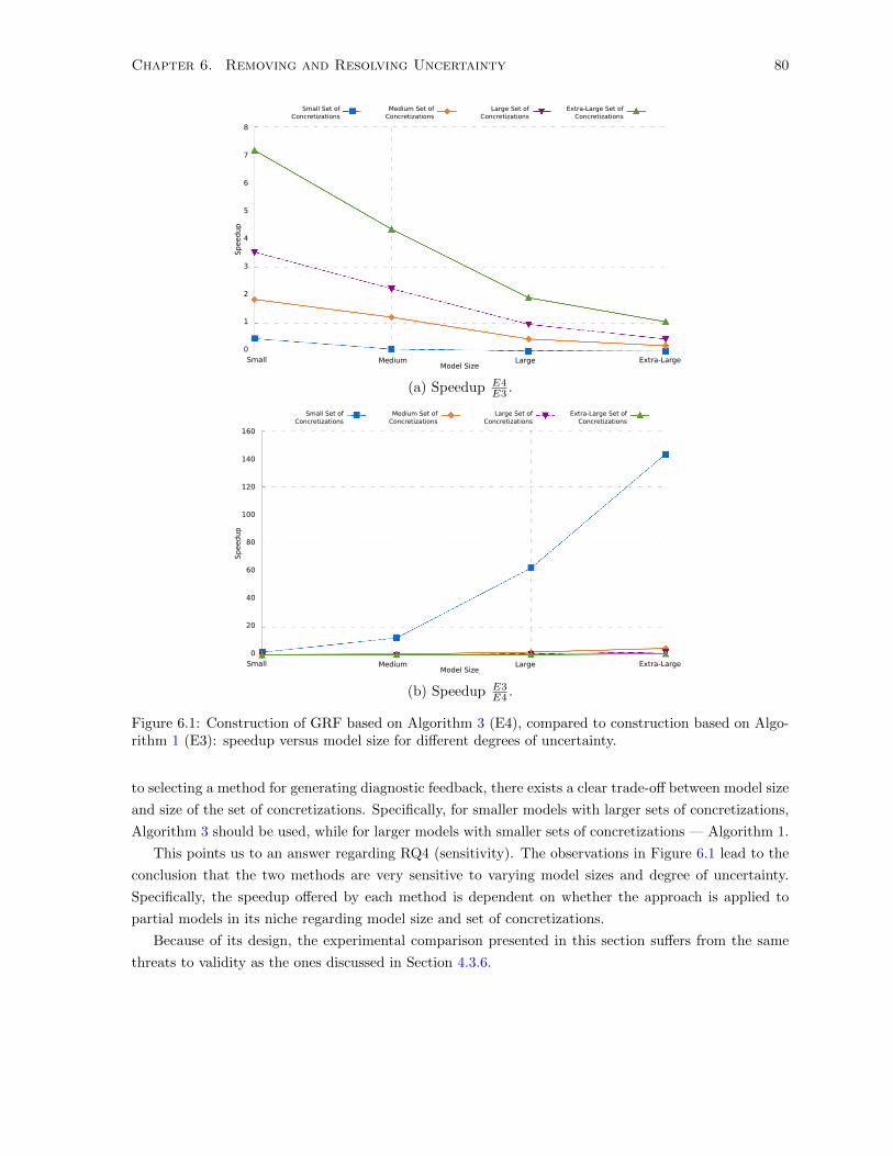
Chapter 6. Removing and Resolving Uncertainty 80
Small Set of Concretizations
Medium Set of Concretizations
Large Set of Concretizations
Extra-Large Set of Concretizations
Sp
eed
up
Model SizeSmall Medium Large Extra-Large
0
1
2
3
4
5
6
7
8
(a) Speedup E4E3 .
Small Set of Concretizations
Medium Set of Concretizations
Large Set of Concretizations
Extra-Large Set of Concretizations
Sp
eed
up
Model SizeSmall Medium Large Extra-Large
0
20
40
60
80
100
120
140
160
(b) Speedup E3E4 .
Figure 6.1: Construction of GRF based on Algorithm 3 (E4), compared to construction based on Algo-rithm 1 (E3): speedup versus model size for different degrees of uncertainty.
to selecting a method for generating diagnostic feedback, there exists a clear trade-off between model size
and size of the set of concretizations. Specifically, for smaller models with larger sets of concretizations,
Algorithm 3 should be used, while for larger models with smaller sets of concretizations — Algorithm 1.
This points us to an answer regarding RQ4 (sensitivity). The observations in Figure 6.1 lead to the
conclusion that the two methods are very sensitive to varying model sizes and degree of uncertainty.
Specifically, the speedup offered by each method is dependent on whether the approach is applied to
partial models in its niche regarding model size and set of concretizations.
Because of its design, the experimental comparison presented in this section suffers from the same
threats to validity as the ones discussed in Section 4.3.6.

Chapter 6. Removing and Resolving Uncertainty 81
6.3 Related Work
Refinement In software engineering, refinement generally means an operation that elaborates some
artifact (e.g., a program, a model, a specification) [Wirth, 1971]. In essence, given an artifact, refinement
creates a new one that is less abstract. In the literature, we encounter two notions of refinement that
are contradicting albeit subtly different.
On the one hand, in the context of formal methods and, specifically, software specification, refinement
is understood as increasing the requirements of a specification. For example, in refinement calculi [Mor-
gan, 1990], refinement can be accomplished by strengthening a specification’s post-condition or weakening
its pre-condition. In the context of partial behavioural formalisms, such as Modal Transition Systems
(MTSs), refinement entails creating a new MTS with a subset of the traces of the original [Larsen and
Thomsen, 1988]. In both cases, a refined specification admits fewer implementations that the original.
In that sense, refinement is understood as removal of behaviour.
On the other hand, in the context of model-driven engineering, refinement is understood as a process
by which implementation details are added to a model expressed at a high level of abstraction [Sendall and
Kozaczynski, 2003]. This is typically done using vertical model transformations [Mens and Gorp, 2006],
such as code generation. Refinement is thus addition of (low level) behaviour. Model Driven Architecture
(MDA) relies heavily on this notion of refinement; however, it also encompasses the “removing” notion
of refinement for “internal refinements”, i.e., transformations that create models at the same level of
abstractions, while preserving semantics [Paige et al., 2005].
In the context of partial modelling, refinement, both in its manual and its property-driven flavours,
is understood as an operation that removes uncertainty, without changing levels of abstraction. In that
sense it is consistent with MDA’s “internal refinements”, albeit addressing a different concern. However,
as discussed in detail in Section 4.1.1, an important difference between partial model refinement and
other forms of “removing” refinement, such as behavioural model refinement, is that its focus is on
preserving structure, rather than behaviour (traces).
Set-reducing operations. Uncertainty resolution is an example of an operation that, given an artifact
encoding a set of models, produces a new one that encodes a subset of the original. As discussed in
Section 3.5, such artifacts are found in formalisms such as software product line engineering (SPLE),
megamodelling and metamodelling
In SPLE, staged configuration [Czarnecki et al., 2004] is a method for incrementally making choices
about which features to include in a product. This is achieved by stepwise reducing the set of possible
configurations of the input feature model. This is done systematically using six different specialization
steps, each one implementing a way to remove a configuration choice. These steps are formalized using
context-free grammars [Czarnecki et al., 2005] and are implemented in the FeaturePlugin tool for the
Eclipse platform [Antkiewicz and Czarnecki, 2004].
Metamodels are also understood as abstractions of sets of instance models. A method typically
used to reduce the set of instances of a metamodel is the addition of constraints [Karsai et al., 2000],
using a language such as the Object Constraint Language (OCL) [Object Management Group, 2006b].
A different approach is to enable the creation of metamodel sub-types. There are various approaches
for creating model subtypes [Guy et al., 2012], mainly focusing on achieving model substitutability,
especially in the context of model transformations. Metamodel pruning is a dual to subtyping, aiming
to create metamodel super-types [Sen et al., 2009].

Chapter 6. Removing and Resolving Uncertainty 82
Megamodels are used to model the macroscopic view of software development. The elements of a
megamodel are themselves models, interconnected with various macro-relations [Favre and NGuyen,
2005; Salay et al., 2009]. In that sense, it is an abstraction of a set of models. Reducing this set (in order
to, for example, create task-specific views) can be accomplished with model slicing [Blouin et al., 2011;
Kagdi et al., 2005]. Since megamodels are themselves models, it is possible to use submodel extraction
techniques [Carre et al., 2013].
6.4 Summary
In this chapter we described the resolution of uncertainty in partial models. A partial model is a transient
artifact, created when the modeller lacks sufficient information to make informed decisions. When such
information becomes available, the modeller can incorporate it in her partial model by reducing the size
of its set of concretizations.
In order to create support for systematic resolution of uncertainty, we have operationalized the
definition of partial model refinement given in Section 3.1 by defining two refinement approaches: manual
decision making and property-driven refinement.
In manual decision making, the modeller incorporates the newly acquired information in the partial
model by making decisions about whether to include or not individual partial model elements that
are annotated with Maybe. This is done using the formally defined operators Keep, Drop (specifically,
DropVertex and DropEdge), respectively.
Instead of editing the diagram of a partial model using operators, property-driven refinement reduces
the set of its concretizations declaratively. In this case, the modeller expresses the newly acquired
information as a property. A refinement is then constructed by appropriately combining the property
with the partial model’s May formula. Property-driven refinement is used in Chapter 4 for diagnosis,
by creating “diagnostic cores”, i.e., refinements encoding the subset of concretizations that violate some
property of interest.
The algorithm for producing user-friendly representations of refinements generated using properties
requires the expensive computation of the “backbone” of the May formula. We conducted an experi-
mental evaluation to study the feasibility and sensitivity of this method of property-driven refinement.
To do this, we compared the method that uses backbone computation to a brute-force method that
enumerates all concretizations of interest and then uses Algorithm 3 to encode them in a partial model.
We have found that the different approaches work best for different combinations of model size and size
of the set of concretizations.
In Chapter 7, we introduce a methodological approach that contextualizes uncertainty resolution in
the software lifecycle with respect to the rest of partial model operations.

Chapter 7
A Methodology for Uncertainty
Management
In this chapter, we investigate the implications of uncertainty management with partial models on
software engineering methodology. We outline the lifecycle of uncertainty management, identifying its
different phases from modelling to resolution. This allows us to contextualize each of the partial modelling
operations defined in previous chapters and so to put together a coherent methodological framework for
uncertainty management. We illustrate our approach using the Model Driven Architecture (MDA)
as a non-trivial example of adapting a software engineering methodology to incorporate uncertainty
management. Finally, we present Mu-Mmint, an interactive modelling tool for uncertainty management
in software development.
The rest of the chapter is organized as follows. In Section 7.1, we introduce the “Uncertainty
Waterfall”, an abstract timeline of uncertainty in software artifacts. In Section 7.2, we use the phases
of the Uncertainty Waterfall to describe the usage context of each partial modelling operation. In
Section 7.3, we exemplify this approach by applying it to the Model Driven Architecture (MDA) software
methodology. In Section 7.4, we present Mu-Mmint, an Eclipse-based tool for managing partial models.
We present related work in Section 7.5 and conclude in Section 7.6.
7.1 The Uncertainty Waterfall
The main premise of this thesis is that once uncertainty appears in the development process, a developer
should attempt to capture it in a special kind of software artifact, called a partial model. Using partial
models, the developer can continue working while avoiding decisions that, in the absence of enough
information, would be premature. When sufficient information is available, the developer systematically
refines the partial model, such that the new information resolves the encoded uncertainty.
In this section, we introduce an abstract model for capturing this lifecycle, that is intrinsic to uncer-
tainty management. This model is called “Uncertainty Waterfall” and presents an idealized timeline of
partial model use. It is shown in Figure 7.1 and it consists of three stages: Articulation of uncertainty,
Deferral of decisions, and Resolution of uncertainty.
We discuss each one in more detail below.
83

Chapter 7. A Methodology for Uncertainty Management 84
Articulation
Deferral
Resolution
Figure 7.1: The Uncertainty Waterfall: an idealized timeline of uncertainty management.
Articulation stage:
This stage is the entry point of uncertainty management: a developer is uncertain about some
aspect of her model due to insufficient information. The main goal during this stage is therefore to
change the model, so that it reflects the developer’s uncertainty. During this stage, the degree of
uncertainty in the model increases as the developer encodes in a partial model the different possible
ways to resolve her uncertainty. These are encoded as concretizations of the partial model.
Deferral stage:
In this stage, the main goal is to avoid premature decision making, while still being able to make
use of software engineering techniques. To do that, the developer uses the partial model as the
primary development artifact. The developer must therefore use versions of such techniques that
have been appropriately lifted so that they are applicable to partial models. During this stage the
degree of uncertainty in the model remains unchanged. This is a fundamental property that lifted
tasks must preserve.
Resolution stage:
This stage begins when more information becomes available. The developer incorporates this new
information into the partial model in a systematic way. During this stage, the degree of uncertainty
in the partial model is reduced to reflect the newly acquired information. The ultimate result of
this stage is a model without any partiality, i.e., a concretization of the original partial model.
The succession of these stages follows a decreasing degree of uncertainty. Uncertainty is introduced
during the Articulation stage; it remains stable during the Deferral stage, and is reduced during the
Resolution stage. We show this schematically in Figure 7.2, as a level of uncertainty present in the
Articulation Deferral Resolution
Uncertainty
Time
Figure 7.2: Degree of uncertainty in different stages of the Uncertainty Waterfall.

Chapter 7. A Methodology for Uncertainty Management 85
doWork
newInformation
moreUncertainty
newUncertainty
moreWork
Articulation
Deferral
Resolution
moreInformation
Figure 7.3: The Extended Uncertainty Waterfall.
software models plotted over time.
We have used the name “Uncertainty Waterfall” in direct analogy with the Waterfall model for
software development [Sommerville, 2007]. We wish to underscore that, like the traditional Waterfall
model, the Uncertainty Waterfall is an abstraction of an inherently messy process. It should not be
misunderstood as a rigid prescription of a strict succession of stages, where an initial explication of
uncertainty is necessarily followed by a series of partial models of monotonically decreasing uncertainty
that culminates in a single concretization. Similarly, the plot in Figure 7.2 is also an abstraction. We
offer the Uncertainty Waterfall model as an intuitive description of the stages of uncertainty management
and the dependencies between them. In fact, the stages may overlap or be used in different orders. A
more realistic model is the Extended Uncertainty Waterfall, shown in Figure 7.3, that includes backward
transitions from later to earlier stages.
The Uncertainty Waterfall, shown in Figure 7.3, contains the following transitions between stages of
uncertainty management:
doWork (Articulation→Deferral)
Once the developer has completed expressing uncertainty in her software artifacts, she can use her
partial models to perform software engineering tasks. This transition is triggered once there is no
more uncertainty to express and the developer needs to continue working.
newInformation (Deferral→Resolution)
If new information becomes available, the developer can use it to resolve all or part of her uncer-
tainty. This transition is triggered if the developer is in a position to resolve some of the uncertainty
and wishes to do so.
moreWork (Resolution→Deferral)
If uncertainty is only partially resolved, the developer can continue performing lifted engineering
tasks while the remaining uncertainty persists. For example, the developer may perform a veri-
fication task, use the results to resolve some of the uncertainty, and then continue working with
refined partial model. This transition is triggered once no more uncertainty can be resolved and
the developer needs to continue working.
newUncertainty (Deferral→Articulation)
In the course of her work with partial models, the developer might encounter additional points of
Chapter 7. A Methodology for Uncertainty Management 86
uncertainty. For example, while already working with a partial model, she may become uncertain
about some design decision for which there was previously no uncertainty. This transition is
triggered when the developer faces the need to express further uncertainty in her software artifacts.
moreUncertainty (Resolution→Articulation)
The developer might need to articulate additional uncertainty immediately following a resolution.
Similarly to the transition newUncertainty, this transition is triggered when the developer faces
the need to express further uncertainty in her software artifacts.
moreInformation (Articulation→Resolution)
The developer might acquire information that allows her to resolve some uncertainty immediately
following articulation. Similarly to the transition newInformation, this transition is triggered if
the developer is in a position to resolve some of the uncertainty and wishes to do so.
In addition to these transitions, we also allow Undo transitions between any two stages. For example,
the transition Undo(Resolution→Articulation) allows the developer undo some refinement in order to
explore different alternatives, while the transition Undo(Articulation→Resolution) allows the developer
to revert to a previous a more concrete version of her artifacts if she decides there is no benefit to
articulating a particular point of uncertainty. Undo transitions are triggered whenever the developer is
not satisfied with the immediately previous transition she took.
The backward links to the Articulation stage can also be the result of eliciting possible solutions
from a previously open design decision. For example, in the PtPP scenario, the developers were initially
faced with uncertainty about the design decision: what policy is followed when leeching ends?. This
is an open-ended question and as such outside the scope of this thesis (cf. the discussion of the limits
of our approach in Section 1.3). However, in our scenario the PtPP developers elicited three acceptable
solutions to this design decision (“selfish”, “benevolent”, and “compromise”), thus reducing the question
to uncertainty about selecting one of them. The backward transitions to the Articulation stage, therefore
allow this process of gradual elicitation of specific alternatives to an open-ended decision point.
The combination of the transitions newInformation and moreWork captures the fact that reso-
lution of uncertainty is not always immediate (i.e., producing a concrete, non-partial model in one step)
but rather that the Deferral and Resolution stages can be interleaved. This interleaving represents the
gradual removal of uncertainty. For example, the developer might apply a transformation to her model,
then resolve some of the uncertainty, check a property, apply a second transformation, and so on.
Finally, we note that the Uncertainty Waterfall also illustrates the fundamentally transient nature of
partial models: they are created when uncertainty is encountered, used as primary development artifacts
in the presence of uncertainty and are ultimately discarded, collapsing to a single, concrete model.
In the following, we use the Uncertainty Waterfall to contextualize the different partial model oper-
ators described throughout the thesis. Whenever we refer to the Uncertainty Waterfall, we mean the
extended version.
7.2 Uncertainty Management Operators
In this thesis, we propose an approach for managing uncertainty in software models by doing model
management [Bernstein, 2003] of models that contain uncertainty, i.e., partial models. The Extended
Uncertainty Waterfall allows us to identify the three distinct usage contexts (Articulation, Deferral,

Chapter 7. A Methodology for Uncertainty Management 87
Table 7.1: Operator Construct
Description Create a partial model from a given set of concrete models that are alternativeresolutions to uncertainty.
Inputs A set of non-partial models.Outputs A partial model.
Usage context The developer has at her disposal a known, fully enumerated set of alternativemodels, but has insufficient information about which of the models is best suitedfor her purpose.
Preconditions No partial model exists. The set of models must be known and fully enumerated.Postconditions The resulting partial model is in Graphical Reduced Form (GRF) and its set of
concretizations is exactly the set of input models.Limitations The developer must have the full knowledge of the input set.
Implementation The operator is realized using Algorithm 3, described in Section 3.4.
Table 7.2: Operator MakePartial
Description Create a partial model from a given concrete model by introducing uncertaintyto it.
Inputs A concrete model and an informal description of uncertainty.Outputs A partial model.
Usage context The developer uses the informal description of uncertainty and her intuition abouthow it should be expressed in the given model.
Preconditions No partial model exists.Postconditions The input model is a concretization of the output partial model.
Limitations Effectiveness depends on the intuition of the developer.Implementation The task is done manually, using the tooling described in Section 7.4.
Resolution) in which developers work with partial models. In section, we describe the uncertainty
management operators that pertain to each stage.
Each operator is described in terms of: (a) its name, (b) a high level description of its functionality,
(c) its inputs and outputs, (d) a description of the development setting in which it is meaningful to invoke
it, (e) its preconditions and postconditions, (f) its limitations in terms of effectiveness or usability, and
(g) the section in the thesis where its implementation is described in detail.
7.2.1 Articulation stage
In this stage operators aim at explicating the developer’s uncertainty about some design decision. Inputs
to articulation operators are therefore inherently informal and subjective. We distinguish three such
operators: Construct, MakePartial, and Expand.
The operator Construct creates a partial model from a set of concrete models, as described in
Table 7.1.
The Construct operator assumes that the developer has full knowledge of the set of concretizations
before invoking it. However, the articulation process can also be manual, requiring the intuition of the
developer to appropriately capture the space of possibilities in the partial model. This is done using the
operator MakePartial, described in Table 7.2.
If uncertainty is encountered while the developer is already working with a partial model, the operator

Chapter 7. A Methodology for Uncertainty Management 88
Table 7.3: Operator Expand
Description Introduce additional uncertainty to a partial model.Inputs A partial model.
Outputs A partial model.Usage context The developer encounters new uncertainty during the Deferral or Resolution
stages of the Extended Uncertainty Waterfall.Preconditions Some uncertainty has already been explicated in the partial model.
Postconditions The input partial model is a refinement of the output.Limitations Effectiveness depends on the intuition of the developer.
Implementation The task is done manually, using the tooling described in Section 7.4.
Table 7.4: Operator Transform
Description Apply a transformation to a partial model ensuring that all concretizations arecorrectly transformed.
Inputs A partial modelOutputs A partial model
Usage context The developer wishes each concretization to be transformed but does not wish toenumerate them all and do it for each one individually.
Preconditions None.Postconditions The set of concretizations of the output partial model is exactly the same as
if the input partial model had been broken down to its set of concretizationsusing the operator Deconstruct, then each concretization in that set had beentransformed individually, and then a partial model had been constructed fromthat set using the operator Construct.
Limitations The model transformation must be expressed as graph rewriting system (i.e., aset of graph rewriting transformation rules).
Implementation The operator is realized by the technique described in Section 5.2.
Expand, described in Table 7.3, allows expanding the existing partial model with the new possibilities.
The common characteristic of the operators of the Articulation stage is that the size of the set of
concretizations increases.
7.2.2 Deferral stage
The aim of operators in this stage is to facilitate decision deferral: if a developer can accomplish software
engineering tasks using partial models, then there is no need to prematurely remove uncertainty. We
therefore lift software engineering operators such they can be used with partial models, without affecting
the degree of uncertainty. We identify two such operators: Transform, and Verify.
The operator Transform, described in Table 7.4, allows developers to apply a model transformation
to a partial model such that all it concretizations are correctly transformed, albeit without having to
enumerate them.
The operator Verify, described in Table 7.5, is used to determine whether a partial model satisfies
a syntactic property.
Following verification, the developer may want to perform diagnostics, as described in Chapter 4.
Since diagnostic operations appropriately remove uncertainty to illuminate parts of the set of the input
partial model’s concretizations, they are discussed in the next section.

Chapter 7. A Methodology for Uncertainty Management 89
Table 7.5: Operator Verify
Description Check whether a partial model satisfies a property.Inputs A partial model, a property.
Outputs A value from the set {True,False,Maybe }.Usage context A developer is interested in determining whether a property is satisfied by some,
all or none of the concretizations of the partial model.Preconditions None.
Postconditions If the property is satisfied by all, none or some of the partial model’s concretiza-tions, then the output is True, False, and Maybe respectively.
Limitations The property is syntactic, i.e., its verification does not require knowledge of thesemantics of the partial model’s base language.
Implementation The operator is realized by the technique described in Section 4.1.
Table 7.6: Operator Deconstruct
Description Produce the set of concretizations of a given partial model.Inputs A partial model
Outputs A set of concrete modelsUsage context The developer needs to perform a task on each concretization of the input partial
model and no lifted version of the task exists.Preconditions None
Postconditions The output set contains exactly the set of concretizations of the input partialmodel.
Limitations High cost.Implementation The operator can be implemented by passing the partial model’s May formula to
an All-Solutions SAT solver [Grumberg et al., 2004].
During the deferral stage if some software engineering operation (in addition to the ones described
above) is required, then it needs to be appropriately lifted. For arbitrary operations, correct lifting
generally depends on the semantics of the base language and is thus outside the scope of this thesis.
It is however always possible (albeit expensive) to enumerate all concretizations, apply the non-lifted
operation to each concretization separately, and then merge the results using Construct. We thus also
introduce the operator Deconstruct, described in Table 7.6, that, given a partial model, creates its
set of concretizations. This can be accomplished by passing the partial model’s May formula to an All-
Solutions SAT solver [Grumberg et al., 2004]. All-Solutions SAT solvers are special purpose reasoning
engines that specialize in efficiently computing all satisfying valuations of a boolean formula. Thus, the
solver will enumerate all satisfying valuations of the May formula, which can then be translated into
models, using the approach described in Section 2.1.2.
Unlike operators in the Articulation and Resolution stages, that increase and reduce the degree of
uncertainty in partial models respectively, operators in the Deferral stage do not affect the degree of
uncertainty.
7.2.3 Resolution stage
Operators at this stage incorporate new information to a partial model, thus reducing its degree of
uncertainty. All the operators can produce either a new partial model that refines the original, or a

Chapter 7. A Methodology for Uncertainty Management 90
Table 7.7: Operator Decide
Description Make decisions about whether to Keep or Drop individual Maybe elements froma partial model.
Inputs A partial model and an informal description of information that resolves uncer-tainty.
Outputs A (potentially singleton) partial model.Usage context The developer uses the informal description of newly acquired information, as
well as her intuition about how it should be incorporated in the input partialmodel.
Preconditions None.Postconditions The output partial model is a refinement of the input partial model.
Limitations The developer may only use the atomic operations Keep, DropEdge, DropVertex.Implementation The operator is realized by the technique described in Section 6.1.1.
Table 7.8: Operator Constrain
Description Create a partial model with a subset of the concretizations of the input partialmodel such that all its concretizations satisfy a property of interest.
Inputs A partial model, a property.Outputs A partial model.
Usage context The developer has determined that concretizations of the input partial modelthat do not satisfy the input property are not valid ways to resolve uncertaintyand should thus be excluded.
Preconditions None.Postconditions The output partial model refines the input partial model.
Limitations This operator is subject to the same limitations as Verify.Implementation The operator is realized using the technique described in Section 6.1.2.
non-partial model, i.e., a concretization of the original. We describe two classes of operators for this
stage. On the one hand, the Decide and Constrain operators incorporate new information obtained
by the developer. Using them, the developer can resolve (partially or completely) the open questions
that prompted the creation of partial models during the Articulation stage. On other hand, the diag-
nostic operators GenerateCounterExample, GenerateExample, and GenerateDiagnosticCore
produce feedback following an invocation of the Verify operator. They remove uncertainty from the
input partial model in order to produce subsets of its concretizations to appropriately illuminate the
results of verification.
The Decide operator, described in Table 7.7, allows the developer to manually make decisions about
which elements should and should not remain in the model. The Constrain operator, described in
Table 7.8, allows narrowing the set of concretizations of a partial model to a subset that satisfies some
property of interest.
We define three diagnostic operators. The operator GenerateCounterExample, described in Ta-
ble 7.9 creates a concretization that functions as a witness as to why a partial model does not satisfy some
property of interest. The operator GenerateExample, described in Table 7.10, creates a concretization
that functions as a witness as to why a partial model can satisfy some property of interest, depending on
how uncertainty is resolved. The operator GenerateDiagnosticCore, described in Table 7.11, creates
a partial model that encodes the subset of concretizations of the input partial model that do not satisfy

Chapter 7. A Methodology for Uncertainty Management 91
Table 7.9: Operator GenerateCounterExample
Description Create a non-partial model that illustrates why a partial model does not satisfya property.
Inputs A partial model, a property.Outputs A concrete model.
Usage context A developer wants to diagnose why a partial model does not satisfy a property,i.e., why the result of Verify is not True.
Preconditions The result of the operator Verify using the input partial model and the inputproperty is Maybe, or False.
Postconditions The output model is a concretization of the input partial model and satisfies theinput property.
Limitations This operator is subject to the same limitations as Verify.Implementation The operator is realized by the technique described in Section 4.2.1.
Table 7.10: Operator GenerateExample
Description Create a non-partial model that illustrates why a partial model may satisfy aproperty.
Inputs A partial model, a property.Outputs A concrete model.
Usage context A developer wants to diagnose why a partial model may satisfy a property, i.e.,why the result of Verify is not False.
Preconditions The result of the operator Verify using the input partial model and the inputproperty is Maybe, or True.
Postconditions The output model is a concretization of the input partial model and satisfies theinput property.
Limitations This operator is subject to the same limitations as Verify.Implementation The operator is realized by the technique described in Section 4.2.2.

Chapter 7. A Methodology for Uncertainty Management 92
Table 7.11: Operator GenerateDiagnosticCore
Description Create a partial model that illustrates why a partial model does not satisfy aproperty.
Inputs A partial model, a property.Outputs A partial model.
Usage context A developer wants to diagnose why a partial model does not satisfy a property,i.e., why the result of Verify is not True.
Preconditions The result of the operator Verify using the input partial model and the inputproperty is Maybe, or False.
Postconditions The output partial model refines (or is equivalent to) the input partial model.The property is not satisfied by any of its concretizations.
Limitations This operator is subject to the same limitations as Verify.Implementation The operator is realized by the technique described in Section 4.2.3.
Articulation
ConstructMakePartialExpand Deferral
TransformVerifyDeconstruct
Resolution
DecideConstrainGenerateCounterExampleGenerateExampleGenerateDiagnosticCore
doWork
newInformation
undoResolution
newUncertainty
moreWork
undoUncertainty
Figure 7.4: Uncertainty management operators overlayed on the Extended Uncertainty Waterfall.
a property of interest. The common characteristic of the operators of the Resolution stage is that the
size of the set of concretizations decreases.
We summarize the set of uncertainty management operators by overlaying them on the Uncertainty
Waterfall in Figure 7.4. Specifically, the operators Construct, MakePartial, and Expand are part of
the Articulation stage, the operators Transform, Verify, and Deconstruct are part of the Deferral
stage, and the operators Decide, Constrain, GenerateCounterExample, GenerateExample, and
GenerateDiagnosticCore are part of the Resolution stage.
7.3 Application: Uncertainty Management in MDA
In this section, we illustrate how uncertainty management can be incorporated into existing software
engineering methodologies. Specifically, we apply our approach to the Model Driven Architecture
(MDA) [Object Management Group, 2014] methodology for software development. We identify the
sources of unertainty in MDA and show how the Uncertainty Waterfall can be used to weave uncertainty
operators in the overall process.
As described in Section 2.4, MDA organizes software development in terms of three architectural
Chapter 7. A Methodology for Uncertainty Management 93
layers, representing hierarchical levels of abstraction. Models at the top layer model the business domain
and are called “computation independent models” (CIMs). In each layer, developers create models that
are independent of lower-level details. Models at lower levels of abstraction are derived automatically
using transformations. These “vertical” transformations combine upper-layer “platform independent
models” (PIMs) with descriptions of the “platform” of the target layer, to create “platform specific
models” (PSMs). Transformations are also used “horizontally”, i.e., within a single layer, to produce
derivative representations of PIMs.
In the following, we list the main sources of uncertainty in MDA and describe how the operators of
the Uncertainty Waterfall can be used to manage it. Specifically, in MDA, uncertainty can arise:
(a) while creating the PIM models of each layer,
(b) from insights gained from derivative representations of PIMs,
(c) in the description of platforms,
(d) in the choice of platform, and
(e) in transformation models.
Additionally, uncertainty can be transmitted vertically: if the PIM and/or the platform model is partial,
the generated PSM should also be partial.
Uncertainty in PIM creation. While working within a particular layer to produce a PIM, the
developer may encounter design decisions for which they have insufficient information. For example,
while creating a CIM at the topmost architectural layer to model the business context, developers
might be uncertain about choosing a scope, i.e., deciding what domain concepts should or should not
be considered in the business model. For concepts that are selected for inclusion to the CIM, further
uncertainty can arise about how to best capture their interdependencies, e.g., choosing between is-a and
has-a relationships.
Explicating such uncertainty can be done using any Articulation operator. For models at the topmost
layer (CIMs), the Expand operator will only be used after entering the Articulation stage via the
transition newUncertainty. For models at lower layers, the Expand operator can be used if the
developer is expanding upon partial models generated from vertical transformations. During the Deferral
stage, the PIM can be used as a basis for the derivation of alternative representations (as partial models)
using Transform and can be the subject of verification for structural correctness using the operator
Verify. The results of verification can be used to do further diagnosis in the Resolution stage, while
additional information can be employed to apply the operators Decide and Constrain.
Uncertainty in derivative representations. MDA allows the use of horizontal transformations
within an architectural layer, in order to facilitate the derivation of alternative representations of existing
PIMs. A different representation might expose modelling options and alternatives that were not easily
discernible in the original format. This is possible at all three architectural layers.
Uncertainty can be articulated using the MakePartial operator. The Expand operator can also
be used since a derived representation can result from applying the Transform operator to a partial
PIM. Further insights can be gained by invoking the Verify operator and the diagnostic operators.
Chapter 7. A Methodology for Uncertainty Management 94
The operator Transform can be used to generate additional derivative models. Since alternative rep-
resentations are derivative artifacts, developers may prefer to avoid invoking resolution operators such
as Decide and Constrain for them. Instead, uncertainty can be propagated back to the PIM using
the Transform operator. Decisions should then be made on the partial PIM and new versions of the
derived representations generated afresh.
Uncertainty about the content of the platform model. Vertical PIM to PSM transformations
require models that describe the target platform as input. Developers could face uncertainty about the
contents of such platform models if developers lack familiarity with a newly adopted platform, if the
construction of the platform takes place in parallel with the construction of the application, or if the
platform is configurable but the developers are unsure about choosing configuration options. Since the
implementation layer is at the lowest level of abstraction, this issue only affects the top two architectural
layers.
Since platform models are not generated using higher level models, the Articulation of uncertainty
for them is identical as with CIMs, described above. Since platform models do not partake in horizontal
transformations, it is not meaningful to apply to them the Transform operator for such transformations.
However, uncertainty in the platform obviously affects downstream artifacts. Since the correctness of
platform models is crucial for PIM/PSM transformations, developers may rely heavily on the Verify
operator and the respective diagnostic operators (GenerateCounterExample, etc.). Resolution of
uncertainty can be accomplished with any of the relative operators but, since correctness is a major
concern, developers may end up relying more on the Constrain operator.
Uncertainty about platform selection. If multiple platform models are available, developers might
be unsure which ones to choose. Such uncertainty could be caused by a rapidly changing software
ecosystem, due to shifting managerial decisions about prioritizing technological platforms, or due to the
complexity arising from working with different subcontractors. This issue affects the top two architectural
layers.
Uncertainty about choosing a platform is articulated using the Construct operator to create a partial
model encoding the available options. To handle the case where the set of possible platforms needs to
be expanded or contracted, developers can invoke the Deconstruct operator, perform any additions or
removal and then invoke Construct again. During the Deferral stage, developers can use the Verify
operator to perform sanity checks on the partial platform model. The diagnostic operators and the
operator Constrain can then be used to appropriately limit the set during the Resolution stage.
Uncertainty in transformation models. Uncertainty can also arise during the construction of
various model transformations used in MDA. For example, given the task of translating a higher-level
concept in a lower level platform, a developer might be uncertain about selecting a target lower-level
concept.
Since MDA transformations are themselves models, expressing and resolving uncertainty is accom-
plished using the Articulation and Resolution operators, respectively. However, there is currently no
technique for executing partial transformation models. Struber et al. have studied transformations
that contain variability [Struber et al., 2015]. Since, as discussed in Section 3.5.3, uncertainty and vari-
ability share some conceptual characteristics, their work may provide a way to leverage uncertainty in
transformation models during the Deferral stage.

Chapter 7. A Methodology for Uncertainty Management 95
Uncertainty and vertical transformations. The PIM/PSM transition between MDA architectural
layers causes uncertainty to be propagated across layers. We distinguish two propagation directions:
downstream and upstream. Uncertainty can be propagated downstream, i.e., from higher to lower layers,
during the application of automatic transformations. Uncertainty can also be propagated upstream, i.e.
from lower to higher layers, as a result of insights gained at lower layers that some upper-layer decisions
that were considered certain need to be re-examined.
Downstream propagation of uncertainty occurs when either the PIM or the platform model are partial,
and thus the resulting PSM should also be partial. The propagation occurs during the Deferral stage of
the management of the input artifacts, using the Transform operator to apply vertical transformations.
Upstream propagation of uncertainty occurs when insights are gained at lower levels of abstraction
that have significant impact on higher-level software artifacts. For such propagation to be possible
vertical transformations must be bidirectional [Stevens, 2008]. Such propagation is highly non-trivial
and is the cause of additional uncertainty. For example, there may be several ways to change a logical
model to improve the architectural design based on insights gained at the implementation level. Eramo
et al. have studied the introduction of uncertainty in models from bidirectional transformations and
have built a prototype implementation [Eramo et al., 2014].
In addition to the propagation of uncertainty, uncertainty resolution can also be propagated either
upstream or downstream. Salay et al. have developed an approach for propagating uncertainty reso-
lutions across models, provided that appropriate traceability links are created and maintained [Salay
et al., 2013a].
Other sources of uncertainty. Additional sources of uncertainty can include uncertainty in language
(i.e., metamodel) definition, uncertainty about tool selection, etc. We focus on uncertainty in the MDA
artifacts themselves (i.e., CIMs, PIMs, PSMs, platform models) since other sources of uncertainty are
ultimately also manifested in them. Therefore, even though the above list is not complete, it contains
sources of uncertainty that uncertainty management in the context of MDA must necessarily address.
Lessons learned. We have applied the uncertainty management approach to Model Driven Archi-
tecture, an engineering methodology for creating software systems. The application of uncertainty
management to MDA necessitated the critical examination of the different stages of MDA development
in order to identify sources of uncertainty.
Having identified the main MDA artifacts in which uncertainty arises, we were able to incorporate
the Uncertainty Waterfall in their MDA life-cycle. We also identified that depending on the artifact
and its MDA context, different uncertainty management operators may be relevant. For example, while
uncertainty in PIMs can be articulated with any Articulation operator, the Construct operator is
more useful when dealing with uncertainty about the choice of platform. We also found that further
research is required for expressing and leveraging uncertainty in partial transformation models. Finally,
we identified that effective vertical propagation of uncertainty and uncertainty resolution highlights the
need of bidirectional transformations and traceability links.

Chapter 7. A Methodology for Uncertainty Management 96
Figure 7.5: Screenshot of Mu-Mmint. Left: interactive workspace showing different versions of PtPP.Middle: Graphical partial model Mp2p for PtPP. Model elements that reify solutions in the uncertaintytree are annotated with (M). Right: Decision tree for Mp2p.
7.4 Tool Support
In this section, we present a tool, called Mu-Mmint1, that implements comprehensive management of
models with uncertainty.
Mu-Mmint is an Eclipse-based tool for model management [Bernstein, 2003] of partial models. It was
created as an Integrated Development Environment (IDE) that bundles various uncertainty management
operators in one coherent unit. We illustrate the main features of Mu-Mmint using the PtPP motivating
example, introduced in Chapter 1.
The workspace of Mu-Mmint is an interactive megamodel [Bezivin et al., 2004], shown in the left
panel of Figure 7.5, which allows modellers to create, manipulate and interact with partial models using
the uncertainty management operations from the Uncertainty Waterfall, shown in Figure 7.4.
Articulation stage. Articulating uncertainty in Mu-Mmint is done using the MakePartial and
Expand uncertainty operators. We illustrate this in PtPP. Initially, the team’s design is separated into
known and unknown parts, as shown in Figure 1.2(a). In Mu-Mmint, developers can explicate this
information in a single partial model Mp2p, shown in the middle and right panels of Figure 7.5.
In Mu-Mmint, the May formula is modelled graphically using the uncertainty tree, shown in the
right panel of Figure 7.5. The uncertainty tree consists of a list of decision elements, each of which can
have any number of children representing mutually exclusive alternative solutions. For Mp2p, the tree
contains the three decisions listed in Figure 1.2(a). For each decision, the team explicates the possible
solutions. For example, the decision about the policy when a download completes involves selecting
among three alternative solutions, described in Chapter 1: “benevolent”, “selfish”, and “compromise”.
Assuming that the uncertainty tree of a given partial model P has k decisions {D1, ..., Dk}, that a
given decision Px has n alternative solutions {ADx1 , ..., ADx
n } and that a given alternative solution ADxy has
l model elements, the May formula φP of P is: φP =∧k
x=1 φDx, where φDx
=Choose(φADx1, . . . , φADx
n),
where Choose is a boolean function that returns True if exactly one of its arguments is True. In turn
φADxy
=∧l
z=1 uz, where uz = ez if ez ∈ ADxy and uz = ¬ez if ez ∈ ADx
w −ADxy for w 6= y and e ∈ P . An
example of this construction is given in Appendix D.2.
1Available at: http://github.com/adisandro/mmint

Chapter 7. A Methodology for Uncertainty Management 97
Figure 7.6: Highlighting the elements that reify the “compromise” alternative solution in Mu-Mmint.
The middle panel shows the graphical part of the Mp2p partial model. It consists of a diagram
expressed in the language of partialized state machines, shown in Figure 3.3, that includes Maybe-
annotated elements. These elements reify the various alternative solutions and are included in the final
version of the model only if their respective solution is selected. For example, the state Finishing and
its associated transitions are annotated with (M) and [Compromise] to indicate that they are part of
that particular solution to the policy decision.
To further support the articulation process, Mu-Mmint supports highlighting the elements reifying
a particular solution, as shown in Figure 7.6. Mu-Mmint can also highlight the alternative resolutions
of a decision point, using different colours, as shown in Figure 7.7. These features allow developers to
quickly examine the various possibilities in the partial model.
Deferral stage. Mu-Mmint implements the Verify operator that allows users to check syntactic
properties, such as the property P2 (“no two transitions have the same source and target”) in the PtPP
example. If the result of property checking in Maybe or False, Mu-Mmint allows users to invoke the
GenerateCounterExample operator. For example, Figure 7.8 shows how Mu-Mmint generates the
concretization in Figure 1.4(c), as a counterexample for P2. Mu-Mmint contextualizes the counterex-
ample with respect to the original partial model by greying out unused Maybe elements.
Mu-Mmint also implements the Transform operator, using the Henshin graph transformation lan-
guage and engine [Arendt et al., 2010] to implement lifting as described in Chapter 5. However, support
for the Transform operator in Mu-Mmint is limited, due to the limited expressiveness of the uncer-
tainty tree. Specifically, lifted transformations do not necessarily produce partial models whose May
formulas are expressible as uncertainty trees. Therefore in Mu-Mmint, the May formula of partial mod-
els created as output by lifted transformations is not shown to users graphically. Instead, it is stored as
a raw SMT-LIB [Barrett et al., 2010] string in the workspace megamodel.
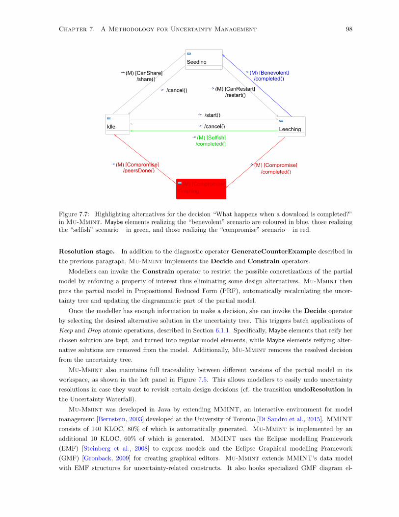
Chapter 7. A Methodology for Uncertainty Management 98
Figure 7.7: Highlighting alternatives for the decision “What happens when a download is completed?”in Mu-Mmint. Maybe elements realizing the “benevolent” scenario are coloured in blue, those realizingthe “selfish” scenario – in green, and those realizing the “compromise” scenario – in red.
Resolution stage. In addition to the diagnostic operator GenerateCounterExample described in
the previous paragraph, Mu-Mmint implements the Decide and Constrain operators.
Modellers can invoke the Constrain operator to restrict the possible concretizations of the partial
model by enforcing a property of interest thus eliminating some design alternatives. Mu-Mmint then
puts the partial model in Propositional Reduced Form (PRF), automatically recalculating the uncer-
tainty tree and updating the diagrammatic part of the partial model.
Once the modeller has enough information to make a decision, she can invoke the Decide operator
by selecting the desired alternative solution in the uncertainty tree. This triggers batch applications of
Keep and Drop atomic operations, described in Section 6.1.1. Specifically, Maybe elements that reify her
chosen solution are kept, and turned into regular model elements, while Maybe elements reifying alter-
native solutions are removed from the model. Additionally, Mu-Mmint removes the resolved decision
from the uncertainty tree.
Mu-Mmint also maintains full traceability between different versions of the partial model in its
workspace, as shown in the left panel in Figure 7.5. This allows modellers to easily undo uncertainty
resolutions in case they want to revisit certain design decisions (cf. the transition undoResolution in
the Uncertainty Waterfall).
Mu-Mmint was developed in Java by extending MMINT, an interactive environment for model
management [Bernstein, 2003] developed at the University of Toronto [Di Sandro et al., 2015]. MMINT
consists of 140 KLOC, 80% of which is automatically generated. Mu-Mmint is implemented by an
additional 10 KLOC, 60% of which is generated. MMINT uses the Eclipse modelling Framework
(EMF) [Steinberg et al., 2008] to express models and the Eclipse Graphical modelling Framework
(GMF) [Gronback, 2009] for creating graphical editors. Mu-Mmint extends MMINT’s data model
with EMF structures for uncertainty-related constructs. It also hooks specialized GMF diagram el-

Chapter 7. A Methodology for Uncertainty Management 99
Figure 7.8: Visualizing a counterexample to property P2 in Mu-Mmint.
ements and views to represent partial models. Mu-Mmint uses the Z3 SMT solver [De Moura and
Bjørner, 2011] for performing reasoning tasks, and adapts parts of the Henshin [Arendt et al., 2010]
engine for lifted graph transformations.
The main limitation of Mu-Mmint is the expressiveness of the visual syntax used to represent uncer-
tainty in partial models. Our original intent was to realize the graphical syntax introduced in [Famelis,
M. and Santosa, S., 2013] which was designed using the theory of visual notations developed by D.
Moody [Moody, 2009]. This was not possible because of our reliance on GMF. While GMF allows
easy integration of existing model editors to Mu-Mmint, it only supports a limited visual vocabulary.
To overcome this, we introduced the concept of the uncertainty tree, as shown in the right panel of
Figure 7.5. This approach attempts to ameliorate the limitations of GMF by using a separate dialog,
exclusively dedicated to modelling uncertainty at a higher level of abstraction. This idea followed from
a preliminary empirical study with human participants [Famelis, M. and Santosa, S., 2013] that pointed
us to the need to elevate decisions and alternative solutions to first class concepts in partial modelling.
The uncertainty tree approach is less expressive than the fully fledged propositional logic, which results
in problems in supporting the Transform operator. However, since it has been shown that humans can
graphically create and manipulate many useful formulas [Czarnecki and Wasowski, 2007], this represents
a trade-off between usability and expressive power. Resolving this trade-off is ultimately dependent on
the usage-specific requirements of the context in which Mu-Mmint is deployed.
7.5 Related Work
The management of uncertainty in the software lifecycle ultimately involves the systematic management
of a representation of a set of possibilities. A similar need to manage the lifecycle of abstractions of sets
of artifacts arises in related software engineering disciplines such as variability management and design
space exploration.

Chapter 7. A Methodology for Uncertainty Management 100
Design space exploration (DSE) [Saxena and Karsai, 2010; Apvrille et al., 2006] is a technique for
systematically traversing a space of design choices in order to identify functionally equivalent designs
that best satisfy a given set of desired constraints. The DSE process follows a series of steps that is
typically described as follows: (1) A reference model is created to represent the requirements and
constraints of the desired design. (2) Using the reference model, the developer derives a set of criteria
with which to evaluate designs. (3) A model of the design space is created. (4) The developer employs
various algorithms to traverse the design space and generate candidate designs. Tools such as Alloy can
be used to automate this step [Kang et al., 2011]. (5) Each candidate design is measured against the
evaluation criteria. (6) Desirable candidate designs are chosen based on whether they optimally satisfy
the evaluation criteria.
The DSE process has certain similarities with the Uncertainty Waterfall: the first two steps resemble
the mental process by which a developer identifies a source of uncertainty; the third step corresponds
to the Articulation stage of uncertainty managament and the final step – to the Resolution stage. The
intermediate stage between Articulation and Resolution differs between DSE and uncertainty manage-
ment. In DSE, decisions are not deferred; rather they are algorithmically explored to produce candidate
designs. However, in uncertainty management, the goal is to allow developers to avoid making such
decisions. Thus, the focus during this stage is in creating support for lifted engineering tasks that allow
developers to continue working with their artifacts without resolving uncertainty.
The goal of variability management [Pohl et al., 2005] is to create and maintain families of products,
called Software Product Lines (SPLs), that share a common set of features. In direct analogy to the
Uncertainty Waterfall, we can identify three stages of SPL lifecycle: Creation, Maintenance, and Con-
figuration. During SPL creation, the aim is to develop a set of reusable assets that can be combined
to produce individual products [Gomaa, 2004]. A common task during this stage is to reverse engineer
a SPL from a set of existing products that share functionality, albeit in an ad-hoc way. To address
this, various techniques have been developed such as feature location [Rubin and Chechik, 2013], clone
detection [Roy et al., 2009] and others. During the Maintenance phase, variability-aware techniques
are applied to SPLs in order to manipulate the entire set of products without having to enumerate
it. Such techniques include model checking [Classen et al., 2010], type checking [Kastner et al., 2012],
testing [Kastner et al., 2012], model transformations [Salay et al., 2014; Famelis et al., 2015b], and oth-
ers [Midtgaard et al., 2014; Thum et al., 2012]. During the Configuration stage, individual products
are derived from the SPL to address individual customer needs. This is typically done by configuring a
feature model that expresses the allowable combinations of features [Schobbens et al., 2006]. This can
be done either at once or in stages [Czarnecki et al., 2004].
The main methodological difference between variability management and uncertainty management
is that SPLs represent a long term commitment to supporting and maintaining a product family. It is
thus not meaningful to talk about a “Variability Waterfall”: Configuration is not the ultimate endpoint
of variablity management. Rather, it represents a set of tasks that developers expect to perform often
during the lifetime of a SPL. In contrast, partial models are transient artifacts. The Resolution stage of
the Uncertainty Waterfall is an endpoint that represents the expectation that uncertainty is ultimately
removed from software artifacts. Put simply, partial models are built to throw away, whereas SPLs are
built to last.

Chapter 7. A Methodology for Uncertainty Management 101
7.6 Summary
In this chapter, we have investigated the implications of uncertainty management on software engi-
neering methodology. We have introduced the Uncertainty Waterfall model as a high level abstraction
of the lifecycle of uncertainty in software artifacts. The Uncertainty Waterfall model consists of three
stages: 1. during the Articulation stage, developers construct partial models to express their uncertainty,
2. during the Deferral stage, the degree of uncertainty in software artifacts remains unchanged, while
developers use lifted versions of existing operations to perform engineering tasks, 3. finally, during the
Resolution stage, new information is incorporated to resolve uncertainty by refining partial models. De-
velopers transition between these stages based on their engineering needs and the absence or presence
of sufficient information to perform these needs.
We have used the Uncertainty Waterfall to contextualize the various techniques presented throughout
the thesis. We have summarized each technique as an “uncertainty management operator”, and defined
its place within the uncertainty lifecycle in terms of its inputs, outputs, usage context, and conditions
prior to and after their invocation. The techniques for modelling uncertainty presented in Chapter 3
were cast as operators used during the Articulation stage. Techniques for performing verification of
partial models, presented in Chapter 4, and for transforming partial models, presented in Chapter 5,
were used to define the operators of the Deferral stage. Finally, techniques for refining partial models,
presented in Chapter 6, as well as techniques for performing diagnosis, presented in Chapter 4, were
contextualized as operators used during the Resolution stage.
To illustrate our approach, we have investigated uncertainty management in the context of the Model
Driven Architecture (MDA), a software methodology that uses models as the primary development arti-
fact. To do this, we critically examined the different stages of MDA and identified sources of uncertainty.
We then illustrated how the different uncertainty management operators can be used to manage this
uncertainty within the MDA lifecycle.
Finally, we described Mu-Mmint, an interactive Eclipse-based tool that implements uncertainty
management. In Mu-Mmint, implementations of uncertainty management operators from the Uncer-
tainty Waterfall are bundled in a coherent Integrated Development Environment.
In Chapter 8, we illustrate uncertainty management as described by the Uncertainty Waterfall model
in fully worked-out examples.

Chapter 8
Worked-Out Examples
In this chapter, we present non-trivial worked examples to illustrate uncertainty management in complex
software development settings. We structure the presentation of each example along the workflow defined
by the Uncertainty Waterfall model defined in Chapter 7.
In Section 8.1, we present an example of managing uncertainty caused by multiple alternative fixes
to a bug in UMLet, an open source software project. In Section 8.2, we illustrate uncertainty manage-
ment in an example that uses the Object-Relational Mapping transformation benchmark, presented in
Section 5.4. We summarize our findings in Section 8.3.
8.1 UMLet Bug #10
On March 8th, 2011, a software developer under the alias “AFDiaX” submitted a bug report to the issue
tracker of UMLet, an open source Java-based UML drawing tool [Auer et al., 2003]. The bug report,
originally posted on Google Code and since migrated to GitHub as Bug #101, stated:
copied items should have a higher z-order priority
What steps will reproduce the problem?
1. Copy an item (per double-click)
2. Click on the area where the original and the copy are overlapping
3. Move the mouse
What is the expected output? What do you see instead?
Expected: The new copy should be moved
Instead: The original item is moved
Type-Enhancement Component-UI OpSys-All Priority-Low Usability
That is, if the user copies and then pastes an item within the editor at a location where it overlaps
with other existing items, the system does not recognize it as the topmost item, i.e., it does not give it
“z-order priority”.
1Bug #10: https://github.com/umlet/umlet/issues/10, URL accessed on 2015-10-22.
102

Chapter 8. Worked-Out Examples 103
In this section, we use this real world bug to illustrate explicit uncertainty management. Specificially,
we create a fictional but realistic scenario in which the maintainer of UMLet attempts to create a fix
for bug #10. In our scenario, the maintainer is a practitioner of model-driven software development
that uses models as the main artifact for development, relying on code generation to derive the Java
implementation.
In order to fix the bug, the maintainer modifies the UML Sequence Diagram modelling the behaviour
of the system. However, soon after she realizes that her fix created additional problems because she mod-
ified the sequence diagram without properly synchronizing it with the structural aspects (e.g., classes)
of the system. This causes her model to violate certain constraints required by the code generator. In
order to resolve these constraint violations, she uses an automated technique that generates alternative
model repairs [Mens and Van Der Straeten, 2007].
In our scenario, uncertainty arises when the maintainer is unsure about which of these subsequent
repairs to choose because their relative merits are unclear. She would thus like to reason with the set of
alternative repairs to help her make the choice and possibly even defer the decision until more information
is available. In the rest of this section, we show how uncertainty management can be deployed to help
the maintainer, illustrating the use of partial modelling techniques throughout the different stages of the
Uncertainty Waterfall.
Description of bug #10 and the maintainer’s bug fix. In the version of UMLet that was current
at the time that the bug was reported2, the paste functionality was implemented by instantiating the
class Paste and invoking its execute operation. Figure 8.1 shows a fragment of the sequence diagram,
generated from the code using the Borland TogetherJ tool3. The fragment shows execute with the
circled portion representing the fictional bug fix that the maintainer creates.
Although UMLet has 214 classes in total, we restrict ourselves to a slice that is relevant to the Paste
class consisting of 6 classes (in addition to Java library classes). These have a total of 44 operations,
out of which 13 are invoked in Paste. The relevant slice of the UMLet model is captured by model K0,
shown in the Appendix Figure D.1. K0 consists of 63 EMF [Steinberg et al., 2009] model elements, out
of which 43 are EMF references.
In Figure 8.1, the for loop statement block iterates through every item in the clipboard, indexed by
variable e. First, each item’s (x, y) coordinates in the editor window are identified (messages 1.36-1.38).
The item is then added as an element to the editor window, represented by the object pnl, at the
coordinates (x, y) of the drawing plane (messages 1.40-1.41).
The bug is caused because when an item is added to a DrawPanel, its order in the stack of other items
at position (x, y), i.e., its “z-order”, is not set to 0 by default. In our scenario, the maintainer fixes the bug
by creating a transient object positioner (message 1.42). The positioner has a method moveToTop(e)
that is invoked to place the item on top of others, using the library operation setComponentZOrder from
the Swing graphical framework (messages 1.43-1.44). In the diagram, the bug fix is shown encircled by
a dashed line.
2Revision 59 on Google Code, since then migrated to GitHub and available at: https://github.com/umlet/umlet/
commit/f708f57a1fbf98b3b083e583761e9887ea717ef3, URL accessed on 2015-10-22.3http://www.borland.com/us/products/together/, URL accessed 2011-09-30

Chapter 8. Worked-Out Examples 104
self e:GridElement
elem:AddElement
pnl:DrawPanel
positioner
1:execute(handler)
1.36:getX()
1.38:getY()
1.37:*
1.39:*
1.40:AddElement(e,x,y,zoom)
1.41:execute(handler)
1.42:new
1.43:moveToTop(self, e)
1.44:setComponentZOrder(e,0)
handler:DiagramHandler
for *GridElement e:this.entities+
sd: Paste.execute
Figure 8.1: Sequence diagram fragment of the UMLet paste function, depicting the execute operation.The maintainer’s fix for bug #10 is encircled by a dashed line.
8.1.1 Articulation stage
The fix to bug #10 created by the maintainer is conceptually correct but it violates two consistency
rules, defined in [Van Der Straeten et al., 2003], that are required for code generation:
• ClasslessInstance: Every object must have a class.
• DanglingOperation: The operation used by a message in a sequence diagram must be an oper-
ation of the class of the receiving object.
In the maintainer’s bug fix, shown in Figure 8.1, the positioner object violates ClasslessInstance be-
cause it is not associated with any class. Additionally, the message 1.43 in which the operation moveToTop
is invoked violates DanglingOperation because it is not in positioner’s class (since positioner has
no class).
In order to resolve these consistency violations, the maintainer uses an automated technique that
generates alternative model repairs [Mens and Van Der Straeten, 2007]. The technique proposes the
following repair strategies for ClasslessInstance:
• RC1: Remove the object.
• RC2(obj): Replace the object with an existing object obj that has a class.
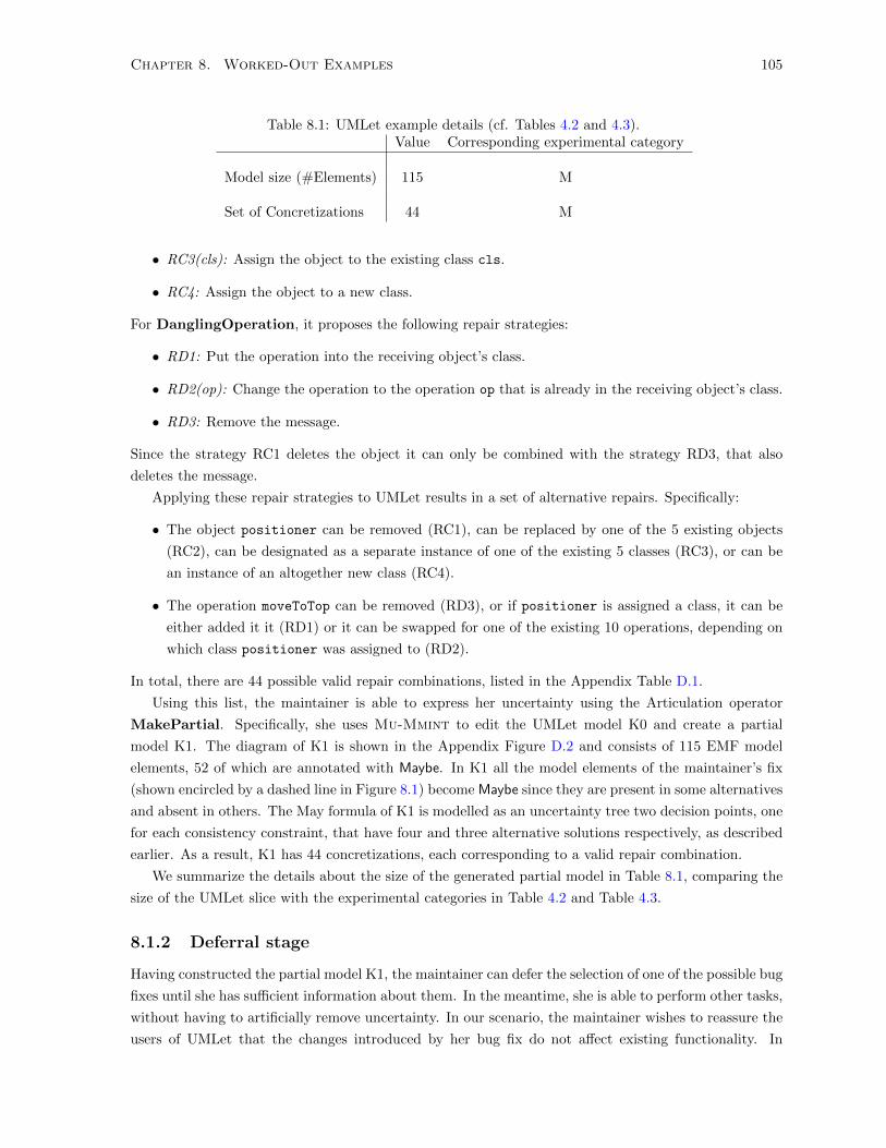
Chapter 8. Worked-Out Examples 105
Table 8.1: UMLet example details (cf. Tables 4.2 and 4.3).Value Corresponding experimental category
Model size (#Elements) 115 M
Set of Concretizations 44 M
• RC3(cls): Assign the object to the existing class cls.
• RC4: Assign the object to a new class.
For DanglingOperation, it proposes the following repair strategies:
• RD1: Put the operation into the receiving object’s class.
• RD2(op): Change the operation to the operation op that is already in the receiving object’s class.
• RD3: Remove the message.
Since the strategy RC1 deletes the object it can only be combined with the strategy RD3, that also
deletes the message.
Applying these repair strategies to UMLet results in a set of alternative repairs. Specifically:
• The object positioner can be removed (RC1), can be replaced by one of the 5 existing objects
(RC2), can be designated as a separate instance of one of the existing 5 classes (RC3), or can be
an instance of an altogether new class (RC4).
• The operation moveToTop can be removed (RD3), or if positioner is assigned a class, it can be
either added it it (RD1) or it can be swapped for one of the existing 10 operations, depending on
which class positioner was assigned to (RD2).
In total, there are 44 possible valid repair combinations, listed in the Appendix Table D.1.
Using this list, the maintainer is able to express her uncertainty using the Articulation operator
MakePartial. Specifically, she uses Mu-Mmint to edit the UMLet model K0 and create a partial
model K1. The diagram of K1 is shown in the Appendix Figure D.2 and consists of 115 EMF model
elements, 52 of which are annotated with Maybe. In K1 all the model elements of the maintainer’s fix
(shown encircled by a dashed line in Figure 8.1) become Maybe since they are present in some alternatives
and absent in others. The May formula of K1 is modelled as an uncertainty tree two decision points, one
for each consistency constraint, that have four and three alternative solutions respectively, as described
earlier. As a result, K1 has 44 concretizations, each corresponding to a valid repair combination.
We summarize the details about the size of the generated partial model in Table 8.1, comparing the
size of the UMLet slice with the experimental categories in Table 4.2 and Table 4.3.
8.1.2 Deferral stage
Having constructed the partial model K1, the maintainer can defer the selection of one of the possible bug
fixes until she has sufficient information about them. In the meantime, she is able to perform other tasks,
without having to artificially remove uncertainty. In our scenario, the maintainer wishes to reassure the
users of UMLet that the changes introduced by her bug fix do not affect existing functionality. In

Chapter 8. Worked-Out Examples 106
particular, she focuses on the behaviour of the Paste command, wishing to show that the property U1
holds, regardless of the details about how bug #10 was fixed:
U1: Whenever an item is pasted, a new item is created in the editor window.
For her model to satisfy property U1, it must have: (a) the message paste from the Paste class to
the ClipBoard class to obtain the pasted GridElement e, (b) the message cloneFromMe to e in order
to create a new GridElement copy to be pasted, and finally (c) the instantiation of a new AddElement
command object to add the item to the editor window. The maintainer uses the operator Verify to
show that this is the case. To do this, she first encodes the property U1 in logic, creating the formula
φU1. The grounded version of φU1, expressed in SMT-LIB [Barrett et al., 2010] is shown in the Appendix
Figure D.5. She then invokes the Verify operator with K1 and φU1 as inputs.
In Mu-Mmint, the invocation of Verify follows the decision procedure described in Chapter 4.
First, the queries F+(SD,K1, U1) and F−(SD,K1, U1) are constructed, where “SD” stands for the well-
formedness constraints of sequence diagrams. Their encoding for this example is shown in the Appendix
Figure D.4. The two queries are then given as inputs to the Z3 SMT solver [De Moura and Bjørner,
2011] and the results are interpreted according to Table 4.1. In our scenario, the Verify operator returns
True, indicating that all concretizations of K1 satisfy the property. This is reasonable, since neither the
bug fix, nor the automatically generated consistency repairs repairs affected that part of the model.
To triangulate the experimental findings described in Section 4.3.5, we compared this method of per-
forming Verify with the “classical” approach of checking the property for each concretization separately,
as described in Section 4.3.1. The comparison showed that the version of Verify using partial models
was 3.84 times faster than the alternative.
Since checking property U1 yielded True, the maintainer is able to reassure her users that the al-
ternative bug fixes do not break the paste functionality. Having determined that U1 is not a factor in
deciding how to resolve uncertainty, she now returns her attention to the property U2:
U2: Each item that is pasted from the clipboard must have z-order=0.
It was the violation of this property that originally caused bug #10.
In her model, ensuring that pasted elements are assigned the correct z-order is done by invoking the
method setComponentZOrder of the class DrawPanel with the item e and the z-order 0 as parameters.
Again, the maintainer invokes the operator Verify to check that this is the case. She encodes U2 in
logic, creating the formula φU2, the grounded version of which is shown in the Appendix Figure D.3
along with the relevant well-formedness condition. In this case the operator Verify yields the result
Maybe, indicating that some but not all of the concretizations satisfy the property. Compared to classical
verification, checking U2 with partial models was 1.95 times faster.
8.1.3 Resolution stage
The maintainer is alarmed by the verification result since it indicates that not all concretizations of K1
actually fix bug #10. To understand why that is the case, she uses the operator GenerateCounterEx-
ample with K1 and U2 as inputs. The operator finds the concretization K2, shown in the Appendix
Figure D.6, which is the result of applying the consistency repairs RC1 and RD3, i.e., deleting the model
elements the maintainer added to K0 to fix the bug in the first place.

Chapter 8. Worked-Out Examples 107
To ensure that bug #10 is fixed, the maintainer must refine her partial model, i.e., reduce its set of
concretizations to the subset that satisfies U2. To accomplish this she invokes the operator Constrain
with K1 and U2 as inputs. As described in Section 6.1.2, this entails combining U2 with the May
formula of K1 and then putting the result in Graphical Reduced Form (GRF). In the resulting partial
model K3, the diagram of which is shown in the Appendix Figure D.7, the positioner, as well as the
messages moveToTop, setComponentZOrder, and new (which instantiates the positioner) are no longer
annotated with Maybe. This means that they must exist in each concretization of K3. However, all
the edges that have one of these elements as their source are annotated with Maybe. For example, the
positioner object has 6 outgoing class reference edges, all of which are annotated with Maybe. This is
because the decision about what class this object is an instance of has yet to be made. The allowable
combinations of Maybe elements are captured in the May formula φK3. Specifically, φK3 encodes the
repair combinations 2 through 44 from the Appendix Table D.1.
To triangulate the experimental findings described in Section 6.2.3, we compared alternative ways
of computing the GRF of K3, as described in Section 6.2.1. We found that computing the GRF using
Algorithm 3 than using Algorithm 1 results in a 0.45 slowdown. This is comparable with the finding
of a 0.525 S4/3 slowdown (cf. Figure 6.1(a)) for a model with size in the M category and size of set of
concretizations in the M category.
At this point, the maintainer has created a partial model that encodes a set of possible models, all of
which are both valid fixes to bug #10 and consistent with the constraints imposed by the code generator.
She can choose to again defer making a decision, thus entering a second Deferral stage, or to further
resolve uncertainty if she feels she has adequate information to do so.
In our scenario, she chooses the combination of repair options RC4, RD2, which assigns positioner
to a new class NewClass that also has the method moveToTop. To accomplish this, she invokes the
operator Decide, thus creating the concrete model K4, shown in the Appendix Figure D.8.
8.1.4 Summary and lessons learned
Summary. We summarize the UMLet example in Figure 8.2, which superimposes the models and
invocations of uncertainty management operators in the scenario over the Uncertainty Waterfall model.
At the start of the scenario, the maintainer of UMLet received a bug report saying that pasted
elements in the UMLet editor do not have the correct z-order. To fix the bug, she identified a slice of
UMLet that contained the bug, represented by the model K0. In fixing the bug, she realized that her
changes caused two consistency constraints required by the code generator to be violated. She used an
automated technique for generating repairs to these constraints, which resulted in a set of 44 alternative
ways to fix the bug. Not having enough information to choose between them, she entered the uncertainty
Articulation stage and created the partial model K1 using the operator MakePartial on K0. Having
expressed her uncertainty, she entered the Deferral stage, where she used the Verify operator to check
properties of her partial model.
In the process, she found out that K1 contained concretizations which did not really fix the original
bug. She proceeded to remove them from her model, thus entering the Resolution stage. She used the
GenerateCounterExample operator to diagnose why some of the concretizations were not valid fixes.
The counterexample K2 showed her that a particular combination of strategies to repair the consistency
violations effectively undid her original repair. To address this, she used the operator Constrain to
remove the offending concretizations, thus creating the partial model K3 that only contained valid fixes.

Chapter 8. Worked-Out Examples 108
doWork
newInformation
Articulation
MakePartial
K1
Deferral
K1
Verify(U1)True
Verify(U2)Maybe
Resolution
K1
GenerateCounterExample(U2)
K2
Constrain(U2)
K3
Decide
K4
K0
Figure 8.2: Overview of the UMLet example, superimposed over the Uncertainty Waterfall model.
Finally, she chose a particular combination of consistency repairs and used the Decide operator to
resolve all uncertainty in her models, creating the model K4.
Lessons learned. The UMLet example allowed us to work a realistic, non-trivial example through
the stages of the Uncertainty Waterfall. Two main lessons emerged:
1. Articulation of uncertainty requires automated support. During the Articulation stage, we had to
express a large combination of possible repairs as a partial model. Even with the tooling support
provided by Mu-Mmint, the manual construction of the partial model K1 using the MakePartial
operator was tedious and error-prone. In order for the effort expended in constructing a partial
model to be outweighed by the benefits, we need to create additional automated support. This
could be achieved using techniques such as Design Space Exploration [Saxena and Karsai, 2010], by
integrating partial modelling into sketching tools [Mangano et al., 2010; Wuest et al., 2015], or by
mining the social context of development, such as online discussions between developers [Mashiyat
et al., 2014]. We discuss these potential research directions in more detail in Section 9.2.
2. Rigid separation of verification from diagnostic operators is counter-intuitive. In the Uncertainty
Waterfall model, the Verify operator is placed in the Deferral stage, whereas diagnostic operators,
such as GenerateCounterExample, are placed in the Resolution stage. There are good reasons
for this: during Resolution uncertainty is reduced, whereas during Deferral its level remains con-
stant. However, since in practice verification and diagnosis are closely intertwined, it is important
to emphasize that the transition between of stages is not as rigid, even when taking into account
the backward transitions in Figure 7.3.
In addition to the above, the UMLet example allowed us to triangulate the experimental findings
from Chapters 4 and 6. We summarize our observations in Table 8.2. In Table 8.2, each speedup in
the UMLet example is shown next to the corresponding experimental result for models of size M with
M size of concretizations. The observation for U1 is compared with the average of property checks

Chapter 8. Worked-Out Examples 109
Table 8.2: UMLet example observed speedups, compared with experimental observations.Verification Speedup (E2/E1) GRF Construction Speedup (E4/E3)
UMLet example Experiments UMLet example Experiments
Property U1 3.84 2.85 (No GRF construction necessary)Property U2 1.95 1.49 0.45 0.525
that returned True or False, whereas the observations for U2 are compared with those for which the
property check returned Maybe. For verification, the speedups that we observed are slightly higher
than the results observed experimentally using randomly generated inputs (cf. Figure 4.1). For GRF
construction, the observed slowdown was slightly slower (cf. Figure 6.1). We believe that there are
two explanations for these findings: 1. Compared to the generated graphs used for our experiments,
the structure (and therefore the resulting propositional encoding) of the UMLet models is not random.
2. For our experimental evaluation, we used untyped directed graphs because the absence of metamodel
constraints makes the problem harder for the solver to solve. On the other hand, we encoded additional
metamodel constraints for the UMLet example. Overall, these observations lead us to conclude that the
experimental results detailed in Sections 4.3.5 and 6.2.3 constitute a lower bound of the performance of
our approach.
8.2 Petri Net Metamodel
In this section, we take the view of a toolsmith who is tasked with creating a fictional tool, called
ConcMod, for modelling concurrent systems. ConcMod uses Petri nets (PTNs), a powerful formalism
used widely in this domain, first introduced by Carl Petri in 1962 [Petri, 1962]. A succinct description
of PTNs is found in [Jensen and Kristensen, 2015]:
“A Petri net in its basic form is called a place/transition net, or PTN, and is a directed
bi-partite graph with nodes consisting of places (drawn as ellipses) and transitions (drawn
as rectangles). The state of a Petri net is called a marking and consists of a distribution of
tokens (drawn as black dots) positioned on the places. The execution of a Petri net (also
called the “token game”) consists of occurrences of enabled transitions removing tokens from
input places and adding tokens to output places, as described by integer arc weights, thereby
changing the current state (marking) of the Petri net. An abundance of structural analysis
methods (such as invariants and net reductions), as well as dynamic analysis methods (such
as state spaces and coverability graphs), exist for Petri nets.”
p1 p2t1
1 1
p1 p2t1
1 1
Figure 8.3: Example Petri net token game. Left: Transition t1 is enabled. Right: the Petri net afterfiring t1.
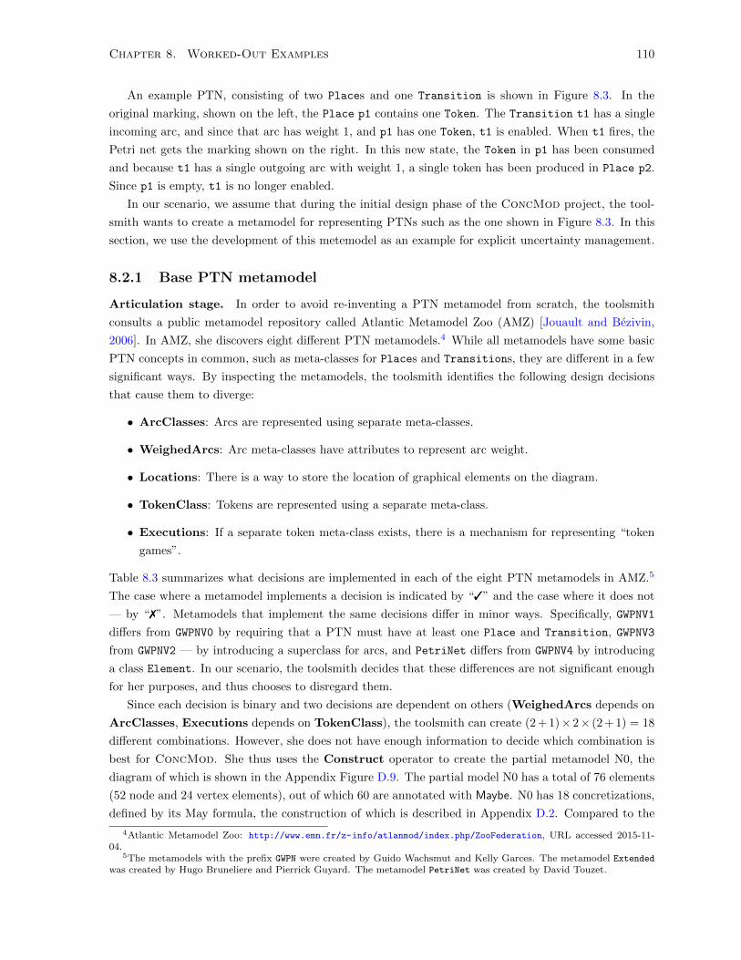
Chapter 8. Worked-Out Examples 110
An example PTN, consisting of two Places and one Transition is shown in Figure 8.3. In the
original marking, shown on the left, the Place p1 contains one Token. The Transition t1 has a single
incoming arc, and since that arc has weight 1, and p1 has one Token, t1 is enabled. When t1 fires, the
Petri net gets the marking shown on the right. In this new state, the Token in p1 has been consumed
and because t1 has a single outgoing arc with weight 1, a single token has been produced in Place p2.
Since p1 is empty, t1 is no longer enabled.
In our scenario, we assume that during the initial design phase of the ConcMod project, the tool-
smith wants to create a metamodel for representing PTNs such as the one shown in Figure 8.3. In this
section, we use the development of this metemodel as an example for explicit uncertainty management.
8.2.1 Base PTN metamodel
Articulation stage. In order to avoid re-inventing a PTN metamodel from scratch, the toolsmith
consults a public metamodel repository called Atlantic Metamodel Zoo (AMZ) [Jouault and Bezivin,
2006]. In AMZ, she discovers eight different PTN metamodels.4 While all metamodels have some basic
PTN concepts in common, such as meta-classes for Places and Transitions, they are different in a few
significant ways. By inspecting the metamodels, the toolsmith identifies the following design decisions
that cause them to diverge:
• ArcClasses: Arcs are represented using separate meta-classes.
• WeighedArcs: Arc meta-classes have attributes to represent arc weight.
• Locations: There is a way to store the location of graphical elements on the diagram.
• TokenClass: Tokens are represented using a separate meta-class.
• Executions: If a separate token meta-class exists, there is a mechanism for representing “token
games”.
Table 8.3 summarizes what decisions are implemented in each of the eight PTN metamodels in AMZ.5
The case where a metamodel implements a decision is indicated by “3” and the case where it does not
— by “7”. Metamodels that implement the same decisions differ in minor ways. Specifically, GWPNV1
differs from GWPNV0 by requiring that a PTN must have at least one Place and Transition, GWPNV3
from GWPNV2 — by introducing a superclass for arcs, and PetriNet differs from GWPNV4 by introducing
a class Element. In our scenario, the toolsmith decides that these differences are not significant enough
for her purposes, and thus chooses to disregard them.
Since each decision is binary and two decisions are dependent on others (WeighedArcs depends on
ArcClasses, Executions depends on TokenClass), the toolsmith can create (2 + 1)× 2× (2 + 1) = 18
different combinations. However, she does not have enough information to decide which combination is
best for ConcMod. She thus uses the Construct operator to create the partial metamodel N0, the
diagram of which is shown in the Appendix Figure D.9. The partial model N0 has a total of 76 elements
(52 node and 24 vertex elements), out of which 60 are annotated with Maybe. N0 has 18 concretizations,
defined by its May formula, the construction of which is described in Appendix D.2. Compared to the
4Atlantic Metamodel Zoo: http://www.emn.fr/z-info/atlanmod/index.php/ZooFederation, URL accessed 2015-11-04.
5The metamodels with the prefix GWPN were created by Guido Wachsmut and Kelly Garces. The metamodel Extendedwas created by Hugo Bruneliere and Pierrick Guyard. The metamodel PetriNet was created by David Touzet.

Chapter 8. Worked-Out Examples 111
Table 8.3: Design decisions in Petri net metamodels from the Atlantic Metamodel Zoo. Each columnrepresents one metamodel.
GWPNV0 GWPNV1 GWPNV2 GWPNV3 GWPNV4 GWPNV5 Extended PetriNet
ArcClasses 7 7 3 3 3 3 3 3
WeighedArcs 7 7 7 7 3 3 3 3
Locations 7 7 7 7 7 7 3 7
TokenClass 7 7 7 7 7 3 3 7
Executions 7 7 7 7 7 7 3 7
categories in Tables 4.2 and 4.3, N0 falls in the S category for model size and the M category for the
size of the set of concretizations. Additionally, N0 has more Maybe elements and fewer concretizations
than any of the partial models used as input to the ORM benchmark, described in Table 5.1.
Deferral Stage: Transformation. Having explicated her uncertainty in the partial model N0, the
toolsmith can defer making a decision about how exactly to design the ConcMod metamodel. In the
meantime, she can use N0 to proceed with other development tasks. In our scenario, the focus of the
toolsmith is turned to the serialization of PTN models. In order to efficiently store PTN models, the
toolsmith wants to use a relational database. She thus needs to create a database schema that allows
her to store instances of PTN models.
Mapping the PTN metamodel to a relational database schema is an instance of the well-known “Ob-
ject Relational Mapping” (ORM) problem. In model-driven software engineering, a typical solution to
the ORM problem involves creating a model transformation that takes a class diagram as input and
produces a relational schema model as output. In our scenario, the toolsmith uses an ORM trans-
formation published in [Varro et al., 2006] that consists of five layered rewrite rules that, given a class
diagram, create a relational schema and traceability links between them. The rules and the input/output
metamodels are shown in Appendix C.
The toolsmith invokes the uncertainty management operator Transform with N0 and the ORM
transformation as inputs. The result is the partial relational schema model N1, consisting of 30 tables.
Overall, N1 has 192 elements (tables, columns, and key references), out of which 184 are Maybe. The
runtime of the transformation was 2.00 seconds and the generated SMT-LIB May formula has the size
of 23.26 kB.
Deferral Stage: Verification. The toolsmith continues working in the presence of uncertainty. Hav-
ing created a partial relational database schema, she decides to investigate whether her schema allows
her to accurately store the graphical diagrams of PTN models. She formalizes this requirement as a
property:
U3: The database must allow storing the diagram coordinates of every graphical PTN construct.
For her database schema to satisfy U3, for each table Ti in N1 that stores some graphical PTN
construct (i.e., the tables Place, Transition, Token, PlaceToTransitionArc, TransitionToPlaceArc)
there must exist a table TLi that maps tuples from Ti to tuples from the table Location. The toolsmith
uses the operator Verify to check whether N1 satisfies U3. To do this, she first encodes the property U3
in logic, creating the formula φU3. The grounded version of φU3, expressed in SMT-LIB [Barrett et al.,
2010], is shown in the Appendix Figure D.11. She then invokes the Verify operator with N1 and φU3 as

Chapter 8. Worked-Out Examples 112
inputs. The result of the property check is Maybe, indicating that U3 may not be satisfied, depending
on how uncertainty is resolved.
Resolution stage. In order to discover the reason why checking U3 on N1 results in Maybe, the
toolsmith uses the diagnostic operators. Using the operator GenerateCounterExample, she discovers
that since the Location table is annotated with Maybe, there exists at least one concretization in which
it does not exist. Since her primary development artifact is the partial metamodel N0, she uses this new
information to refine N0 using the operator Decide to ensure that the class Location is present in all
concretizations. The result is the partial metamodel N2, shown in the Appendix Figure D.12.
Additionally, by invoking the operator GenerateDiagnosticCore with N1 and U3 as inputs,
she discovers that there are no tables mapping tuples of the tables Token, PlaceToTransitionArc,
TransitionToPlaceArc to the table Location. She decides that this is acceptable, since the location
of these graphical elements can be derived from Places and the combination of endpoint Place and
Transition, respectively.
The toolsmith does not have any more information to fully resolve the uncertainty in N2. Addition-
ally, she receives new requirements for ConcMod, which cause her more uncertainty, prompting her to
enter a new uncertainty Articulation stage.
8.2.2 Extended PTN metamodel
Articulation stage. Due to its simplicity, the Petri net formalism lends itself to customization in
order to capture domain-specific concerns. This has lead to the proliferation of Petri net extensions,
which augment the base language with special-purpose constructs. Examples of such Petri net exten-
sions include Coloured PTNs [Jensen, 1987], Hierarchical PTNs [Fehling, 1993], Prioritized PTNs [Guan
et al., 1998], Timed PTNs [Ramchandani, 1974], Stochastic PTNs [Molloy, 1982], and others. In our
scenario, the toolsmith learns that her employer is considering allowing such PTN models to be stored
in ConcMod. However, she does not have enough information about which domain-specific constructs
should be included in the ConcMod metamodel.
Faced with uncertainty about which Petri net extensions to support, the toolsmith uses the operator
Expand on the partial metamodel N2, to create the partial metamodel N3. The uncertainty tree of N3,
shown in the Appendix Figure D.14, contains several new (binary) design decision points:
• ArcKinds: There are different kinds of arcs, such as inhibitor and reading arcs [Murata, 1989].
• Priority: Transitions have priorities [Guan et al., 1998].
• Timed: Transitions are timed [Ramchandani, 1974].
• ColouredTokens: Tokens have values, called “colours” taken from “Colour Sets”, i.e., types [Jensen,
1987].
• Stochastic: Each transitions has a “firing rate” that indicates the probability that it will fire at
every marking [Molloy, 1982].
• Guards: Arcs have guard expressions [Jensen, 1987].
Chapter 8. Worked-Out Examples 113
The decisions Guards, WeighedArcs, and ArcKinds depend on the decision ArcClasses, while
the decisions Executions and ColouredTokens depend on the decision TokenClass. Therefore, the
uncertainty tree allows (1 + 2 × 2 × 2) × (1 + 2 × 2) × 2 × 2 × 2 = 360 concretizations. The model
elements required to implement these design decisions bring the total elements of N3 to 117 elements,
out of which 94 are Maybe. The diagram of N3 is shown in the Appendix Figure D.13. Compared to
the categories in Tables 4.2 and 4.3, N3 falls into the M category for model size and is larger than the
XL category for the size of the set of concretizations. Additionally, N3 has more Maybe elements and
more concretizations than any of the partial models used as input to the ORM benchmark, described in
Table 5.1.
Deferral stage. Having explicated her uncertainty in the partial model N3, the toolsmith again gener-
ates a relational database schema using the ORM transformation. She invokes the uncertainty manage-
ment operator Transform again, this time with N3 and the ORM transformation as inputs. The result
is the partial relational schema model N4, which has 45 tables. In total, N4 has 293 elements (tables,
columns, and key references), out of which 258 are Maybe. The total runtime of the transformation was
114.05 seconds and the generated SMT-LIB May formula is 33.78 kB long.
Resolution stage. Using lifted operations, the toolsmith can continue working in the presence of
uncertainty for as long as necessary. In our scenario, we assume that at some point the toolsmith is
able to resolve all of her uncertainty by making all of the design decisions. Specifically, she uses the
Decide operator with the partial model N3 as input and makes the choice to not implement any of the
domain-specific Petri net extensions, to allow executions to be stored, and to use separate arc and token
meta-classes. These decisions result in the concrete metamodel N5, shown in the Appendix Figure D.15.
8.2.3 Summary and lessons learned.
Summary. We summarize the PTN metamodel example in Figure 8.4, which superimposes the models
and invocations of uncertainty management operators in the scenario over the Uncertainty Waterfall
model.
At the start of the scenario, the toolsmith in charge of creating ConcMod aimed to create a meta-
model for representing Petri nets. She consulted an open repository of metamodels, where she located
eight existing different Petri net metamodels. By analysing these metamodels, she identified five impor-
tant design decisions that are the cause of the differences between them. Not having enough information
to decide how to make these decisions, she used the operator Construct to create the partial metamodel
N0.
Having articulated her uncertainty in N0, the toolsmith entered the Deferral stage. She applied the
ORM transformation to her partial metamodel using the operation Transform, to create a derived
partial relational schema model N1. She then applied the operator Verify to check whether N1 allows
storing the diagrammatic locations of Petri net elements. The result of the check was Maybe, and
prompted her to perform further diagnosis using the diagnostic operators. She discovered that (a) not
all concretizations have a dedicated table for storing locations, and (b) the locations of some of the
diagrammatic elements can be derived from others.
The first diagnostic insight led her to enter the Resolution stage, where she used the newly acquired
information to resolve some of the uncertainty in N0, to ensure that the Location table is present in all

Chapter 8. Worked-Out Examples 114
1: doWork
2: newInformation
Articulation/1
Construct
N0K0K0designdecisions
Deferral/1
N0 Maybe
Verify(U3)Transform
N1
Resolution/1
N0
Decide
N2
3: moreUncertaintyArticulation/2
N2
Expand
N3
Deferral/2
N3
Transform
N4
Resolution/2
N3
Decide
N5
4: doWork
5: newInformation
Figure 8.4: Overview of the PTN metamodel example, superimposed over the Uncertainty Waterfallmodel.
concretizations. To do this, she applied the operator Decide, resulting in the partial metamodel N2.
The second insight led her to re-examine the requirement to store the locations of all elements.
At this point in our scenario, the toolsmith had to consider the possibility of creating support in
ConcMod for representing various Petri net flavours, that add domain-specific modelling constructs to
the base Petri net language. She thus entered a second Articulation stage, where she applied to operator
Expand to the partial metamodel N2, resulting in the partial metamodel N3.
The toolsmith entered a second Deferral stage, where she again invoked the operator Transform to
apply the ORM transformation to the partial model N3, resulting in the new partial relational schema
model N4. Subsequently, the toolsmith was able to remove all uncertainty from her models during a
second Resolution stage, where she used the operator Decide to reduce N3 to the concrete Petri net
metamodel N5.
Lessons learned. In the Petri net metamodel example, we worked with a medium-sized model with
a large set of concretizations and a large percentage of Maybe elements through the different stages of
uncertainty management. Three main lessons arose from this experience:
1. Even though we described the initial articulation of uncertainty in terms of invoking the operator
Construct for the set of all possible metamodel designs, in practice, we had to adopt a slightly
different approach. Specifically, we manually constructed the partial model N0, using the eight
AMZ metamodels and the five design decisions as guidance. This was a different process than
both Construct (which is fully automatic but depends on an enumerated set of alternatives) and
MakePartial (which is manual but depends on a pre-existing concrete model). Rather, in practice,
we ended up adopting elements of both, whereby we manually enumerated a set of possibilities,
using the uncertainty tree as a guide.
2. The number of application sites and the number of Maybe elements in the partial models N0 and
N3 was significantly larger than that of the models used for the ORM benchmark (described in

Chapter 8. Worked-Out Examples 115
Table 5.1). This made the original implementation of our lifted transformation engine extremely
inefficient. We were thus forced to revisit it and implement various optimizations that resulted in
improvements in both runtime and the size of the generated May formula. These improvements
were so dramatic as to render comparison with the benchmark results meaningless. However, during
the implementation of the optimizations, we faced significant challenges in correctly engineering
complex manipulations of large formulas while working with the application programming interface
(API) of the Z3 solver [De Moura and Bjørner, 2011]. This process was extremely error prone and
hard to debug, thus exposing some of the practical difficulties of our lifting strategy, that focuses
on manipulating a single large propositional expression. We contrast this with our experience
implementing lifting for product lines, where individual elements are annotated with “presence
conditions” [Salay et al., 2014; Famelis et al., 2015b]. This makes the implementation of lifting
significantly easier, since instead of manipulating a single large formula, it uses smaller logical
expressions that are localized to specific matching sites.
3. During the first Resolution stage, the toolsmith invoked the Verify operator, which returned
Maybe. However, instead of using the result to constrain the partial model, we found that it was
more appropriate for the toolsmith to change her expectations about the property. This points to
a characterization of properties with modalities, such as “necessary” and “possible”. Responses
to property checks can therefore include either refining the underlying model or changing the
modality of the property. In current work, we are investigating such property modalities and
appropriate responses to the verification of such properties in the context of product lines with
uncertainty [Chechik et al., 2016].
8.3 Summary
In this chapter, we have applied the techniques described in the rest of the thesis to non-trivial, fully
worked-out examples. We have used the Uncertainty Waterfall model, introduced in Chapter 7, to
illustrate two scenarios of explicit uncertainty management.
The experience gained from these examples has illustrated the capabilities of our approach and
exposed some of its limitations. In Chapter 9, we build upon this experience to outline potential
directions for future research.
Chapter 9
Conclusion
This chapter concludes the thesis. In Section 9.1, we summarize the key points of the thesis and in
Section 9.2, we discuss limitations of our approach and outline directions for future work to address
them.
9.1 Summary
In this thesis, we have presented an approach for helping developers avoid premature commitments while
designing software systems. Such situations arise when developers face uncertainty about the content of
their software artifacts. Since existing software engineering languages, tools, and methodologies do not
support working in the presence of uncertainty, developers are forced to either refrain from using them or
to make provisional decisions and attempt to keep track of them in case they need to revisited. While the
first approach leads to under-utilization of resources, the second risks potentially costly re-engineering
efforts in case the otherwise artificial removal of uncertainty proves premature.
Instead, we have proposed an approach for deferring decisions which developers are not ready to
make. The approach entails carefully managing the lifecycle of uncertainty in software artifacts, while
adapting engineering tasks so that they can be performed in the presence of uncertainty. We captured
this process in the Uncertainty Waterfall, described in Chapter 7, which is a model for the management of
the lifecycle of uncertainty. This lifecycle consists of three stages: Articulation, Deferral, and Resolution.
Uncertainty management operations pertinent to each stage were presented in detail in Chapters 3, 4
and 5, and 6, respectively.
In Chapter 3, we presented an approach for articulating uncertainty using partial models, a formalism
for compactly and exactly representing sets of possibilities. In partial models, uncertainty about selecting
a possible design is expressed by annotating elements of a base model as “Maybe” while a propositional
May formula constrains their possible combinations, called concretizations. Creating such combinations
is done through a process of structure-preserving refinement, which also forms the basis for defining
the formal semantics of partial models. We introduced a partial model construction algorithm and two
equivalent “reduced forms”, suited for different usage settings. We also described and evaluated the
user-friendliness of the partial model notation and introduced a partialization process for adapting the
metamodel of the base language to support expressing uncertainty.
In Chapter 4, we described automated verification for partial models. We defined the meaning of
116

Chapter 9. Conclusion 117
partial model property checking and explained that because partial models have concretization-based
semantics (i.e., are defined through structure-preserving refinement), we scoped our verification technique
to checking syntactic properties. We gave a decision procedure for checking such properties and described
three kinds of feedback that can be generated in order to help developers perform diagnosis. Through
experimental evaluation of our verification approach, we found that partial model verification results in
significant speedup compared to classical verification (i.e., checking the property on each concretization
separately). We also observed that the speedup increases with greater degrees of uncertainty (i.e., larger
sets of concretizations).
In Chapter 5, we introduced the lifting of graph-based model transformations such that they can be
applied to partial models. We formally introduced the concept of lifting: applying a transformation to
a partial model should produce a new partial model which should be the same as if we had transformed
each concretization of the input partial model separately and then merged them back. A corollary to this
definition is that existing transformations do not need to be redefined for partial models. Instead, we
lifted the semantics of model transformation application. We did this through a three-step process : given
a candidate transformation site in a model, we first determine rule applicability using a SAT solver; then
we transform the graphical part of the partial model; finally, we transform the May formula to ensure
that the correctness of lifting is respected. We showed that our process preserves lifting correctness as
well as confluence and termination, two important properties of graph-based model transformations. We
applied our approach to the Object-Relational Mapping, a common benchmark for model transformation
techniques, and discovered there is a trade-off between transformation runtime and the growth of the
May formula of the output.
In Chapter 6, we described how uncertainty is resolved by systematically integrating newly acquired
information to partial models. We introduced two approaches to operationalize partial model refinement:
manual decision making and property-driven refinement. In the former, the modeller incorporates newly
acquired information in the partial model by making decisions about whether to Keep or Drop individ-
ual Maybe elements. In the latter, uncertainty is resolved declaratively, by expressing newly acquired
information as a property. A refinement is then constructed by appropriately combining the property
with the partial model’s May formula. Through experimentation, we evaluated two different approaches
for performing this construction, and found that each works best for different combinations of model
size and size of the set of concretizations.
We combined these techniques in a coherent whole in Chapter 7, where we investigated the impli-
cations of uncertainty management on software engineering methodology. To capture the lifecycle of
uncertainty in software artifacts we introduced the Uncertainty Waterfall model and used it to contex-
tualize the various uncertainty management operators. To illustrate our approach, we applied it to the
Model Driven Architecture (MDA), a software methodology that uses models as the primary develop-
ment artifact. We critically examined the different stages of MDA and identified sources of uncertainty.
We then illustrated how the different uncertainty management operators can be used to manage this un-
certainty within the MDA lifecycle. Finally, we described Mu-Mmint, an interactive Eclipse-based tool
that implements uncertainty management by bundling the implementations of uncertainty management
operators in an Integrated Development Environment for managing partial models.
In Chapter 8, we illustrated the lifecycle of uncertainty management in fully worked-out examples.
The experience gained from working these examples through the lifecycle of uncertainty illustrated the
capabilities of our approach and exposed some of its limitations. We discuss these in the next section,

Chapter 9. Conclusion 118
along with directions for research to mitigate them.
9.2 Limitations and Future Work
The concern for handling uncertainty permeates software development. In this thesis, we have presented
a particular approach for accomplishing this, based on facilitating the deferral of design decisions. We
have thus presented a coherent and minimally complete subset of what should become a comprehensive
theory of uncertainty management. Below we outline several directions for future work in what promises
to be a fruitful area of research.
Balancing deferral, provisionality, and uncertainty avoidance. Developers routinely face design-
time uncertainty in their day-to-day engineering activities. The virtual omnipresence of functional soft-
ware in contemporary society proves they are capable of effectively dealing with it. This is done using
either of the following: (a) development approaches that avoid uncertainty for as long as necessary by
routing around uncertain parts of the developed system, such as lean software development [Poppendieck
and Poppendieck, 2003b], (b) iterative methodologies that embrace provisionality, such as Agile Devel-
opment [Martin, 2003], or (c) ad-hoc handling of provisional decisions based on experience and intuition.
We intend to further investigate the value proposition of explicit uncertainty management with relation
to existing software development practices. To accomplish this, we intend to study the historical data of
software systems in order to identify cases of catastrophic mismanagement of uncertainty. Subsequently,
we will perform post-hoc analysis in order to determine the effectiveness of different uncertainty man-
agement strategies. In addition, we intend to study the integration of explicit uncertainty management
into lean software development, such as the Scrumban methodology [Ladas, 2009]. This will allow us
to either develop mixed strategies, effectively weaving explicit uncertainty management with existing
approaches, or to recognize niche contexts in which it is cost-effective.
Identification of design decisions and elicitation of solutions. In Section 1.3, we scoped our
approach by making two important assumptions: (a) that developers know what they are uncertain
about, and (b) that all decision points are “known unknowns”, i.e., closed questions where developers
are uncertain about choosing one among a well understood finite set of acceptable solutions. Thus, the
uncertainty management operators that we defined for the Articulation stage of the Uncertainty Waterfall
in Section 7.2.1 assume as input either a fully enumerated set of possibilities or an informal description of
how uncertainty should be expressed in partial models. However, in order to use uncertainty management
in the context of real software development, additional support must be provided for (a) identifying
that development has reached a critical design decision such that explicit uncertainty management is
cost-effective, (b) assessing the impact of uncertainty across multiple artifacts, (c) helping developers
elicit a set of acceptable solutions to an open design decision (an “unknown unknown”), and (d) helping
encode them in a partial model.
To address the first two points, we intend to study the identification of design decisions and the
assessment of their impact, by focusing on the socio-technical context in which such decisions are made.
A first step in this direction is to study historical data from existing software projects in order to develop
a theory about when major design decisions occur in the lifecycle of software projects. A potential
approach is to attempt to identify patterns among changes that had significant impact downstream,

Chapter 9. Conclusion 119
such as changes that resulted in a lot of bugs or changes that required a lot of development effort to
be undone. A different approach is to study the social context in which design decisions are made. We
discuss this possibility in more detail in the next paragraph.
To address the latter points, we intend to investigate the use of domain space exploration tech-
niques [Saxena and Karsai, 2010] for synthesizing sets of possibly acceptable solutions. This would
entail mining the development context to identify a set of acceptability criteria and then generating
designs that are equivalent with respect to these criteria. Additional research must investigate ways for
presenting these recommendations to the developers in a user-friendly way.
Leveraging the social context of software development. Software development is an inherently
social process. For example, the first step for addressing a bug report or a feature request is to start
a conversation between the stakeholders of a software project. This way, points of uncertainty in the
solution space can be identified and proposals to resolve them can be explored. However, due to the
fluid nature of such interactions, it is often hard to understand the state of the discussion and its
impact on the quality of actual software artifacts. In [Mashiyat et al., 2014], we proposed to analyze
the utterances of uncertainty in conversations to create business indicators and analytics. These can
help managers of software development teams assess the state of a project, identify pain points and
recommend interventions. The main challenge lies in automatically generating models of the rhetorical
structure of conversations. This entails the use of natural language processing techniques to: (a) identify
utterances of uncertainty and utterances of proposed resolutions, (b) match each point of uncertainty
with its corresponding proposals, (c) recognize when a proposal is accepted as a sufficient resolution of
a point of uncertainty. Additionally, we can map utterances of uncertainty to software artifacts and use
propagation techniques [Salay et al., 2013a] to help developers articulate and/or resolve uncertainty.
Providing a formal back-end for informal modelling. The empirical work of Marian Petre has
shown that one of the most common uses of UML in practice is as an informal “thought tool” during
initial, exploratory, and creative stages of software design [Petre, 2013]. Flexible modelling approaches
focus on this creative aspect of modelling used for software design and aim to create collaborative tools
that emulate whiteboard modelling, thus facilitating the creative process through informal modelling.
Examples of such tools include Calico [Mangano et al., 2010] and Flexisketch [Wuest et al., 2015]. Even
though the models created by flexible modelling tools are inherently ambiguous and incomplete, it is
possible to use them for certain lightweight analysis techniques. For example, partial models can be used
to merge incomplete sketches created by multiple stakeholders in order to provide them with feedback
about their composite model. Another example of lightweight analysis technique is described in [Motta
et al., 2013], where analysis of timed properties of systems with stochastic behaviour using probabilistic
model checking was deployed in Calico [Motta et al., 2013]. Informal modelling is one of the means
that developers use to make sense of situations in which they encounter uncertainty. We intend to
investigate the use of partial models as a back-end for informal modelling tools. The main challenge is
to interpret informal sketches into partial models that capture the intuition of the modellers. Ideally,
users of informal modelling tools should remain unaware of the partial modelling back-end, while still
gaining meaningful feedback generated using partial modelling techniques.
Verification of semantic properties. In Section 4.1.1, we scoped partial model verification to syn-
tactic properties in order to preserve the language independence of our verification approach. However,

Chapter 9. Conclusion 120
certain semantic properties can be “unrolled” and then checked structurally using bounded model check-
ing [Clarke et al., 2001]. Unrolling entails rewriting looping model structures up to a bounded number
k of iterations. The resulting model structurally models those traces that iterate over the loop up to k
times. It is thus possible to prove whether a semantic property holds within the given bound. Adapt-
ing this technique for partial models depends on correctly lifting the unrolling operation. We intend
to use the technique for lifting graph-rewriting model transformations described in Chapter 5 as the
basis for lifting unrolling. A potential challenge is the automatic generation of graph-rewriting rules for
performing unrolling, given the semantics of a behavioural modelling language.
Partial model execution. In Section 7.3, we identified that one potential source of uncertainty in
MDA is in the construction of model transformations. Since MDA transformations are also models,
expressing and resolving uncertainty can be accomplished using the techniques described in Chapters 3
and 6, respectively. We noted, however, that in order for MDA practitioners to effectively practice
decision deferral, we must also lift transformation execution, and pointed to work by [Struber et al., 2015]
as a potential source of inspiration. This notion can be generalized to other kinds of partial models whose
base language is executable. For example, since the execution of Petri nets can be simulated using graph
rewriting [Ehrig and Padberg, 2004], we can envision the execution of partial Petri nets using lifted graph
transformations. An obvious challenge is the state space explosion problem, as subsequent execution
steps diffuse uncertainty throughout the initial Net. We intend to investigate under what conditions
it is efficient to execute partial models, what kinds of reasoning can be performed with partial model
execution traces, and what insights can be gained. One potential approach is to identify appropriate
abstractions of the partial model’s Propositional Reduced Form (PRF) in order to leverage symbolic
execution techniques.
Improving partial model usability. In [Famelis, M. and Santosa, S., 2013], we introduced a par-
tial modelling notation that was intentionally designed based on D. Moody’s usability theory of no-
tations [Moody, 2009]. This notation significantly influenced the creation of the “uncertainty tree”
modelling sub-language of Mu-Mmint (which also had to take into account existing technological con-
straints). The uncertainty tree abstraction makes it possible to model uncertainty without having to
use propositional logic. In addition, it provides a way to capture uncertain decisions as a first-class
artifact. This way, the rationale for why a particular element is annotated as Maybe is also captured
in the partial model. This, however, comes at a cost to expressiveness which is necessary for applying
lifted transformations, since their output is not necessarily expressible using uncertainty trees. In the
future, we intend to investigate striking a balance between usability and expressiveness. Feature mod-
elling [Schobbens et al., 2006] is a potential source of inspiration, especially given that we have been
able to successfully adapt transformation lifting for feature model-based annotative product lines [Salay
et al., 2014].
Uncertainty and Variability. Variability management techniques have proliferated in industry to
such a degree that it is now not uncommon for a company to maintain multiple product lines at once.
The increasing complexity of features, variation points and domain artifacts requires more sophisticated
ways of expressing and reasoning with questions such as “If we include this feature, will all products
satisfy that property?”, “What are the implications of mapping this feature to that piece of code?”. In
such contexts, the synergy between uncertainty and variability modelling (essentially, the combination

Chapter 9. Conclusion 121
of existential and universal quantification over power-sets of possibilities) can provide a powerful way to
articulate and reason with complicated business scenarios. In current work [Chechik et al., 2016], we are
developing a technique for performing verification of properties on product lines that contain points of
uncertainty, as well as a methodology for responding to verification results.
Similar synergies arise in the field of dynamically adaptive systems (DASs) [Esfahani and Malek,
2012]. In DASs, design decisions are made at run-time to adapt to changes in the environment in which
the software system operates. In fact, DASs are often understood as dynamic product lines [Bencomo
et al., 2008]; thus many of the synergies between uncertainty and variability described above are also
relevant to DAS engineering. In [Ramirez et al., 2012], several sources of design-time uncertainty are
identified for DASs for which no mitigation strategy currently exists. The techniques presented in this
thesis may be directly applicable in addressing this gap. For example, decision deferral can be used
to mitigate uncertainty caused by trying to avoid making “design decisions based on misguided and
subjective preference” [Ramirez et al., 2012].
Lifting industrial-grade transformation languages. The approach for lifting graph-rewriting
transformations presented in Chapter 5 demonstrates the feasibility of simultaneously applying a graph
rewriting rule to an entire set of concretizations. However, industrial-grade model transformation re-
quires languages that are orders of magnitude more complex, with constructs such as control, iteration,
data structures, etc. It is therefore necessary to go beyond simple graph-rewriting. The experience
gained from lifting transformations for partial models has allowed us to adapt this technique to software
product lines [Salay et al., 2014]. Subsequently, we were able to use the lifting of individual graph-rewrite
rules in order to lift parts of DSLTrans. DSLTrans is a full-fledged model transformation language that
combines graph-rewriting with advanced language constructs and is rich enough to implement real-world
transformations [Lucio et al., 2010]. Using the lifted version of the DSLTrans engine, we were able to
execute an industrial-grade model transformation of product lines from the automotive domain [Famelis
et al., 2015b]. In current work, we are expanding lifting to the entire DSLTrans language. We intend to
use the insights and experience gained from this, to lift widely used transformation languages such as
ATL [Jouault et al., 2006].

Bibliography
Abiteboul, S., P. Kanellakis, and G. Grahne, 1987: On the representation and querying of sets of possible
worlds. Proceedings of the 1987 ACM SIGMOD International Conference on Management of Data,
ACM, New York, NY, USA, SIGMOD ’87, 34–48.
URL http://doi.acm.org/10.1145/38713.38724
Aho, A. V., Y. Sagiv, and J. D. Ullman, 1979: Efficient optimization of a class of relational expressions.
ACM Trans. Database Syst., 4, 435–454, doi:10.1145/320107.320112.
URL http://doi.acm.org/10.1145/320107.320112
Akers, S., 1978: Binary decision diagrams. Computers, IEEE Transactions on, C-27, 509–516,
doi:10.1109/TC.1978.1675141.
Ambler, S. W., 2005: The Elements of UML (TM) 2.0 Style. Cambridge University Press.
Anastasakis, K., B. Bordbar, G. Georg, and I. Ray, 2007: Uml2alloy: A challenging model transfor-
mation. Model Driven Engineering Languages and Systems, G. Engels, B. Opdyke, D. Schmidt, and
F. Weil, eds., Springer Berlin Heidelberg, volume 4735 of Lecture Notes in Computer Science, 436–450.
URL http://dx.doi.org/10.1007/978-3-540-75209-7_30
Antkiewicz, M. and K. Czarnecki, 2004: FeaturePlugin: Feature Modeling Plug-in for Eclipse. Proc. of
the 2004 OOPSLA Workshop on Eclipse Technology eXchange, 67–72.
Apvrille, L., W. Muhammad, R. Ameur-Boulifa, S. Coudert, and R. Pacalet, 2006: A uml-based en-
vironment for system design space exploration. Electronics, Circuits and Systems, 2006. ICECS ’06.
13th IEEE International Conference on, 1272–1275.
Arendt, T., E. Biermann, S. Jurack, C. Krause, and G. Taentzer, 2010: Henshin: Advanced Concepts
and Tools for In-place EMF Model Transformations. Proc. of MODELS’10 , 121–135.
Atkinson, C. and T. Kuhne, 2003: Model-driven development: a metamodeling foundation. Software,
IEEE , 20, 36–41, doi:10.1109/MS.2003.1231149.
Auer, M., T. Tschurtschenthaler, and S. Biffl, 2003: A flyweight uml modelling tool for software devel-
opment in heterogeneous environments. Euromicro Conference, 2003. Proceedings. 29th, 267–272.
Bak, K., K. Czarnecki, and A. Wasowski, 2011: Feature and Meta-Models in Clafer: Mixed, Specialized,
and Coupled. Proc. of SLE’10 , 102–122.
Barrett, C., A. Stump, and C. Tinelli, 2010: “The SMT-LIB Standard: Version 2.0”. Proc. of SMT’10 .
122

BIBLIOGRAPHY 123
Ben-David, S., M. Chechik, and S. Uchitel, 2013: Merging partial behaviour models with different
vocabularies. CONCUR 2013 – Concurrency Theory , P. R. D’Argenio and H. Melgratti, eds., Springer
Berlin Heidelberg, volume 8052 of Lecture Notes in Computer Science, 91–105.
URL http://dx.doi.org/10.1007/978-3-642-40184-8_8
Bencomo, N., P. Sawyer, G. S. Blair, and P. Grace, 2008: Dynamically Adaptive Systems are Product
Lines too: Using Model-Driven Techniques to Capture Dynamic Variability of Adaptive Systems.
Proc. of SPLC’12 , 23–32.
Bernstein, P. A., 2003: Applying Model Management to Classical Meta Data Problems. Proc. of
CIDR’03 .
Beydeda, S., M. Book, V. Gruhn, et al., 2005: Model-driven software development , volume 15. Springer.
Bezivin, J., F. Jouault, and P. Valduriez, 2004: On the need for megamodels. In Proc. of OOP-
SLA/GPCE’04 .
Bezivin, J., B. Rumpe, A. Schurr, and L. Tratt, 2006: “Proceedings of the Model Transformations in
Practice Workshop”. Satellite Events at the MoDELS 2005 Conference.
Blouin, A., B. Combemale, B. Baudry, and O. Beaudoux, 2011: Modeling model slicers. Model Driven
Engineering Languages and Systems, J. Whittle, T. Clark, and T. Khne, eds., Springer Berlin Heidel-
berg, volume 6981 of Lecture Notes in Computer Science, 62–76.
URL http://dx.doi.org/10.1007/978-3-642-24485-8_6
Boehm, B., 1991: Software risk management: principles and practices. Software, IEEE , 8, 32–41,
doi:10.1109/52.62930.
Boucher, Q., A. Classen, P. Faber, and P. Heymans, 2010: Introducing TVL, a Text-based Feature
Modelling Language. Proc. of VaMoS’10 , 159–162.
Brooks, F. P., 1995: The Mythical Man-Month. Addison-Wesley Reading, MA.
Bruns, G. and P. Godefroid, 1999: Model Checking Partial State Spaces with 3-Valued Temporal Logics.
Proc. of CAV’99 , 274–287.
Buneman, P., S. Khanna, and W.-C. Tan, 2000: Data provenance: Some basic issues. FST TCS 2000:
Foundations of Software Technology and Theoretical Computer Science, S. Kapoor and S. Prasad,
eds., Springer Berlin Heidelberg, volume 1974 of Lecture Notes in Computer Science, 87–93.
URL http://dx.doi.org/10.1007/3-540-44450-5_6
Buneman, P. and W.-C. Tan, 2007: Provenance in databases. Proceedings of the 2007 ACM SIGMOD
International Conference on Management of Data, ACM, New York, NY, USA, SIGMOD ’07, 1171–
1173.
URL http://doi.acm.org/10.1145/1247480.1247646
Cabot, J., R. Clariso, and D. Riera, 2007: Umltocsp: A tool for the formal verification of uml/ocl
models using constraint programming. Proceedings of the Twenty-second IEEE/ACM International
Conference on Automated Software Engineering , ACM, New York, NY, USA, ASE ’07, 547–548.
URL http://doi.acm.org/10.1145/1321631.1321737

BIBLIOGRAPHY 124
Carre, B., G. Vanwormhoudt, and O. Caron, 2013: From Subsets of Model Elements to Submodels.
Software & Systems Modeling , 1–27, doi:10.1007/s10270-013-0340-x.
Casais, E., 1994: “The Automatic Reorganization of Object Oriented Hierarchies – A Case Study”.
Object Oriented Systems, 1, 95–115.
Chechik, M., K. Czarnecki, M. Famelis, J. Rubin, and R. Salay, 2016: Choices, Choices! Reasoning
About Uncertainty and Variability. In progress.
Chen, P., 1976: The Entity-Relationship Model: Toward a Unified View of Data. ACM Transactions on
Database Systems, 1, 9–36.
Clarke, E., A. Biere, R. Raimi, and Y. Zhu, 2001: Bounded model checking using satisfiability solving.
Formal Methods in System Design, 19, 7–34, doi:10.1023/A:1011276507260.
URL http://dx.doi.org/10.1023/A%3A1011276507260
Classen, P., A.and Heymans, P. Schobbens, A. Legay, and J. Raskin, 2010: Model Checking Lots of
Systems: Efficient Verification of Temporal Properties in Software Product Lines. Proc. of ICSE’10 ,
335–344.
Cohen, B., 2008: The bittorrent protocol specification.
Czarnecki, K. and M. Antkiewicz, 2005: Mapping Features to Models: A Template Approach Based on
Superimposed Variants. Proc. of GPCE’05 , 422–437.
Czarnecki, K. and S. Helsen, 2006: Feature-based survey of model transformation approaches. IBM
Systems Journal , 45, 621–645, doi:10.1147/sj.453.0621.
Czarnecki, K., S. Helsen, and U. Eisenecher, 2004: “Staged Configuration Using Feature Models”. Proc.
of SPLC’04 , 266–283.
Czarnecki, K., S. Helsen, and E. Ulrich, 2005: Formalizing Cardinality-Based Feature Models and Their
Specialization. Software Process: Improvement and Practice, 10, 7 – 29, doi:10.1002/spip.213.
Czarnecki, K. and A. Wasowski, 2007: Feature diagrams and logics: There and back again. Software
Product Line Conference, 2007. SPLC 2007. 11th International , 23–34.
De Moura, L. and N. Bjørner, 2011: “Satisfiability Modulo Theories: Introduction and Applications”.
Commun. ACM , 54, 69–77.
Demuth, B., T. U. Dresden, C. Wilke, and T. U. Dresden, 2009: Model and object verification by using
dresden ocl. Technical University , 81.
Di Sandro, A., R. Salay, M. Famelis, S. Kokaly, and M. Chechik, 2015: MMINT: A Graphical Tool for
Interactive Model Management. Proc. of MODELS’15 .
Dubois, C., M. Famelis, M. Gogolla, L. Nobrega, I. Ober, M. Seidl, and M. Volter, 2013: Research
Questions for Validation and Verification in the Context of Model-Based Engineering. Proc. of MoD-
eVVa’13 , 67–76.
Eclipse, accessed 2013-03-16a: CDO website: http://www.eclipse.org/cdo/ .
URL http://www.eclipse.org/cdo/

BIBLIOGRAPHY 125
— accessed 2013-03-16b: Teneo website: http://wiki.eclipse.org/Teneo/ .
URL http://wiki.eclipse.org/Teneo/
Een, N. and N. Sorensson, 2004: An Extensible SAT-Solver. Theory and Applications of Satisfiability
Testing , Springer, 333–336.
Egyed, A., E. Letier, and A. Finkelstein, 2008: ”Generating and Evaluating Choices for Fixing Incon-
sistencies in UML Design Models”. Proc. of ASE’08 , IEEE Computer Society, 99–108.
Ehrig, H., K. Ehrig, U. Prange, and G. Taentzer, 2006: Fundamentals of Algebraic Graph Transformation
(Monographs in Theoretical Computer Science. An EATCS Series). Springer, 1 edition.
Ehrig, H. and J. Padberg, 2004: Graph grammars and petri net transformations. Lectures on Concur-
rency and Petri Nets, J. Desel, W. Reisig, and G. Rozenberg, eds., Springer Berlin Heidelberg, volume
3098 of Lecture Notes in Computer Science, 496–536.
URL http://dx.doi.org/10.1007/978-3-540-27755-2_14
Eramo, R., A. Pierantonio, and G. Rosa, 2014: Uncertainty in bidirectional transformations. Proceedings
of the 6th International Workshop on Modeling in Software Engineering , ACM, New York, NY, USA,
MiSE 2014, 37–42.
URL http://doi.acm.org/10.1145/2593770.2593772
Esfahani, N. and S. Malek, 2012: Uncertainty in Self-Adaptive Software Systems. Software Engineering
for Self-Adaptive Systems 2, Lecture Notes in Computer Science Hot Topics, R. de Lemos, H. Giese,
H. Muller, and M. Shaw, eds.
Famelis, M., 2012: Uncertainty Management With Partial Models. Proc. of MODELS’12 Doctoral Sym-
posium.
Famelis, M., N. Ben-David, A. Di Sandro, R. Salay, and M. Chechik, 2015a: MU-MMINT: an IDE for
Model Uncertainty. Proc. of ICSE’15 Formal Demonstrations.
Famelis, M., S. Ben-David, M. Chechik, and R. Salay, 2011: “Partial Models: A Position Paper”. Proc.
of MoDeVVa’11 , 1–6.
Famelis, M., M. Chechik, and R. Salay, 2012: “Partial Models: Towards Modeling and Reasoning with
Uncertainty”. Proc. of ICSE’12 .
Famelis, M., L. Lucio, G. Selim, A. Di Sandro, R. Salay, M. Chechik, J. R. Cordy, J. Dingel,
H. Vangheluwe, and Ramesh S, 2015b: Migrating Automotive Product Lines: a Case Study. Proc. of
ICMT’15 .
Famelis, M., R. Salay, and M. Chechik, 2015c: Towards Modeling and Reasoning with Design-Time
Uncertainty. Submitted to TOSEM.
Famelis, M., R. Salay, A. Di Sandro, and M. Chechik, 2013: Transformation of models containing
uncertainty. Proc. of MODELS’13 , 673–689.
Famelis, M. and Santosa, S., 2013: “MAV-Vis: a Notation for Model Uncertainty”. Proc. of MiSE’13 .

BIBLIOGRAPHY 126
Favre, J.-M. and T. NGuyen, 2005: Towards a Megamodel to Model Software Evolution
Through Transformations. Electronic Notes in Theoretical Computer Science, 127, 59 – 74,
doi:10.1016/j.entcs.2004.08.034.
Fehling, R., 1993: A concept of hierarchical petri nets with building blocks. Advances in Petri Nets 1993 ,
G. Rozenberg, ed., Springer Berlin Heidelberg, volume 674 of Lecture Notes in Computer Science, 148–
168.
URL http://dx.doi.org/10.1007/3-540-56689-9_43
Fischbein, D., G. Brunet, N. D’ippolito, M. Chechik, and S. Uchitel, 2012: Weak Alphabet Merging of
Partial Behaviour Models. ACM TOSEM , 21, 9:1–9:47.
Fowler, M. and J. Highsmith, 2001: The agile manifesto. Software Development , 9, 28–35.
Garlan, D., 2010: Software Engineering in an Uncertain World. Proc. of FoSER’10 , 125–128.
Gebser, M., R. Kaminski, A. Konig, and T. Schaub, 2011: Advances in Gringo Series 3. Proc. of
LPNMR’11 , 345–351.
Ghezzi, C., C. Menghi, A. Molzam Sharifloo, and P. Spoletini, 2014: On requirement verification for
evolving statecharts specifications. Requirements Engineering , 19, 231–255, doi:10.1007/s00766-013-
0198-z.
URL http://dx.doi.org/10.1007/s00766-013-0198-z
Gogolla, M., F. Buttner, and M. Richters, 2007: USE: A UML-based specification envi-
ronment for validating UML and OCL. Science of Computer Programming , 69, 27 – 34,
doi:http://dx.doi.org/10.1016/j.scico.2007.01.013, special issue on Experimental Software and Toolk-
its.
URL http://www.sciencedirect.com/science/article/pii/S0167642307001608
Goldsby, H. and B. Cheng, 2010: Automatically discovering properties that specify the latent behavior
of uml models. Model Driven Engineering Languages and Systems, D. C. Petriu, N. Rouquette, and
O. Haugen, eds., Springer Berlin Heidelberg, volume 6394 of Lecture Notes in Computer Science,
316–330.
URL http://dx.doi.org/10.1007/978-3-642-16145-2_22
Gomaa, H., 2004: Designing Software Product Lines with UML: From Use Cases to Pattern-Based
Software Architectures. Addison Wesley Longman Publishing Co., Inc., Redwood City, CA, USA.
Gronback, R., 2009: Eclipse Modeling Project . Addison Wesley.
Grumberg, O., A. Schuster, and A. Yadgar, 2004: Memory efficient all-solutions sat solver and its
application for reachability analysis. Formal Methods in Computer-Aided Design, A. Hu and A. Martin,
eds., Springer Berlin Heidelberg, volume 3312 of Lecture Notes in Computer Science, 275–289.
URL http://dx.doi.org/10.1007/978-3-540-30494-4_20
Guan, S.-U., H.-Y. Yu, and J.-S. Yang, 1998: A prioritized petri net model and its application in dis-
tributed multimedia systems. Computers, IEEE Transactions on, 47, 477–481, doi:10.1109/12.675716.

BIBLIOGRAPHY 127
Guy, C., B. Combemale, S. Derrien, J. Steel, and J.-M. Jezequel, 2012: On Model Subtyping. Proc. of
ECMFA’12 , volume 7349 of LNCS , 400–415.
Hinton, A., M. Kwiatkowska, G. Norman, and D. Parker, 2006: PRISM: A Tool for Automatic Verifica-
tion of Probabilistic Systems. Proc. of TACAS’06 , volume 3920 of LNCS , 441–444.
Hoos, H. H., 2012: Programming by optimization. Commun. ACM , 55, 70–80,
doi:10.1145/2076450.2076469.
URL http://doi.acm.org/10.1145/2076450.2076469
Horkoff, J., R. Salay, M. Chechik, and A. Di Sandro, 2014: Supporting early decision-making in the
presence of uncertainty. Proc. of RE’14 , 33–42.
Ikonen, M., P. Kettunen, N. Oza, and P. Abrahamsson, 2010: Exploring the sources of waste in kanban
software development projects. Software Engineering and Advanced Applications (SEAA), 2010 36th
EUROMICRO Conference on, 376–381.
Islam, S. and S. H. Houmb, 2010: Integrating Risk Management Activities into Requirements Engineer-
ing. Proc. of RCIS’10 , 299–310.
Jackson, D., 2006a: Software Abstractions: Logic, Language, and Analysis. The MIT Press.
— 2006b: Software Abstractions: Logic, Language, and Analysis. MIT Press.
Jensen, K., 1987: Coloured petri nets. Petri Nets: Central Models and Their Properties, W. Brauer,
W. Reisig, and G. Rozenberg, eds., Springer Berlin Heidelberg, volume 254 of Lecture Notes in Com-
puter Science, 248–299.
URL http://dx.doi.org/10.1007/BFb0046842
Jensen, K. and L. M. Kristensen, 2015: Colored petri nets: a graphical language for formal modeling
and validation of concurrent systems. Communications of the ACM , 58, 61–70.
Jones, T. C., 1998: Estimating Software Costs. McGraw-Hill, Inc., Hightstown, NJ, USA.
Jouault, F., F. Allilaire, J. Bezivin, I. Kurtev, and P. Valduriez, 2006: ATL: a QVT-like Transformation
Language. OOPSLA’06 Companion.
Jouault, F. and J. Bezivin, 2006: KM3: A DSL for Metamodel Specification. Formal Methods for Open
Object-Based Distributed Systems, volume 4037 of LNCS , 171–185.
URL http://dx.doi.org/10.1007/11768869_14
Kagdi, H., J. Maletic, and A. Sutton, 2005: Context-free slicing of uml class models. Software Mainte-
nance, 2005. ICSM’05. Proceedings of the 21st IEEE International Conference on, 635–638.
Kang, E., E. Jackson, and W. Schulte, 2011: An approach for effective design space exploration. Foun-
dations of Computer Software. Modeling, Development, and Verification of Adaptive Systems, R. Ca-
linescu and E. Jackson, eds., Springer Berlin Heidelberg, volume 6662 of Lecture Notes in Computer
Science, 33–54.
URL http://dx.doi.org/10.1007/978-3-642-21292-5_3

BIBLIOGRAPHY 128
Kang, K., S. Cohen, J. Hess, W. Novak, and A. Peterson, 1990: Feature-oriented domain analysis
(FODA) feasibility study. Technical report, DTIC Document.
Karsai, G., G. Nordstrom, A. Ledeczi, and J. Sztipanovits, 2000: Specifying Graphical Modeling Systems
Using Constraint-based Meta Models. Proc. of CACSD’00 , 89–94.
Kastner, C. and S. Apel, 2008: Integrating Compositional and Annotative Approaches for Product Line
Engineering. Proc. of GPCE’08 , 35–40.
Kastner, C., S. Apel, T. Thum, and G. Saake, 2012: Type Checking Annotation-Based Product Lines.
ACM TOSEM , 21, 14.
Kastner, C., A. von Rhein, S. Erdweg, J. Pusch, S. Apel, T. Rendel, and K. Ostermann, 2012: Toward
Variability-aware Testing. Proc. of FOSD’12 , 1–8.
Kilby, P., J. Slaney, S. Thiebaux, and T. Walsh, 2005: Backbones and Backdoors in Satisfiability. Proc.
AAAI’05 , 1368–1373.
Krka, I., N. D’Ippolito, N. Medvidovic, and S. Uchitel, 2014: Revisiting compatibility of input-output
modal transition systems. Proc. of FM’14 , C. Jones, P. Pihlajasaari, and J. Sun, eds., Springer
International Publishing, volume 8442 of LNCS , 367–381.
URL http://dx.doi.org/10.1007/978-3-319-06410-9_26
Kuhne, T., 2005: What is a model? Language Engineering for Model-Driven Software Development ,
J. Bezivin and R. Heckel, eds., Internationales Begegnungs- und Forschungszentrum fur Informatik
(IBFI), Schloss Dagstuhl, Germany, Dagstuhl, Germany, number 04101 in Dagstuhl Seminar Proceed-
ings.
URL http://drops.dagstuhl.de/opus/volltexte/2005/23
Ladas, C., 2009: Scrumban - Essays on Kanban Systems for Lean Software Development . Modus Co-
operandi Press, USA.
Larsen, K. G. and B. Thomsen, 1988: “A Modal Process Logic”. Proc. of LICS’88 , 203–210.
Larsen, P., 1991: The Expressive Power of Implicit Specifications. Proc. of ICALP’91 , volume 510 of
LNCS , 204–216.
Lucio, L., B. Barroca, and V. Amaral, 2010: A Technique for Automatic Validation of Model Transfor-
mations. Proc. of MoDELS’10 , Springer, 136–150.
Mangano, N., A. Baker, M. Dempsey, E. Navarro, and A. van der Hoek, 2010: Software design sketching
with calico. Proceedings of the IEEE/ACM International Conference on Automated Software Engi-
neering , ACM, New York, NY, USA, ASE ’10, 23–32.
URL http://doi.acm.org/10.1145/1858996.1859003
Marek, V. W. and M. Truszczynski, 1998: Stable Models and an Alternative Logic Programming
Paradigm. CoRR, cs.LO/9809032.
Marques-Silva, J., M. Janota, and I. Lynce, 2010: On Computing Backbones of Propositional Theories.
Proc. of ECAI’10 , 15–20.

BIBLIOGRAPHY 129
Martin, R. C., 2003: Agile Software Development: Principles, Patterns, and Practices. Prentice Hall
PTR, Upper Saddle River, NJ, USA.
Mashiyat, A., M. Famelis, R. Salay, and M. Chechik, 2014: Using Developer Conversations to Resolve
Uncertainty in Software Development: A Position Paper. Proc. of RSSE’14 .
Mens, T. and P. V. Gorp, 2006: A taxonomy of model transformation. Electronic Notes in Theoretical
Computer Science, 152, 125 – 142, doi:http://dx.doi.org/10.1016/j.entcs.2005.10.021, proceedings of
the International Workshop on Graph and Model Transformation (GraMoT 2005)Graph and Model
Transformation 2005.
URL http://www.sciencedirect.com/science/article/pii/S1571066106001435
Mens, T. and R. Van Der Straeten, 2007: Incremental Resolution of Model Inconsistencies. Proc. of
WADT’06 .
Mens, T., N. Van Eetvelde, S. Demeyer, and D. Janssens, 2005: “Formalizing Refactorings with Graph
Transformations”. Journal of Software Maintenance and Evolution: Research and Practice, 17, 247–
276, doi:10.1002/smr.316.
URL http://dx.doi.org/10.1002/smr.316
Midtgaard, J., C. Brabrand, and A. Wasowski, 2014: Systematic derivation of static analyses for software
product lines. Proceedings of the 13th International Conference on Modularity , ACM, New York, NY,
USA, MODULARITY ’14, 181–192.
URL http://doi.acm.org/10.1145/2577080.2577091
Misra, S. C., V. Kumar, and U. Kumar, 2009: Identifying some important success factors in adopting
agile software development practices. Journal of Systems and Software, 82, 1869 – 1890.
Molloy, M., 1982: Performance analysis using stochastic petri nets. Computers, IEEE Transactions on,
C-31, 913–917, doi:10.1109/TC.1982.1676110.
Monden, Y., 2011: Toyota production system: an integrated approach to just-in-time. CRC Press.
Moody, D., 2009: The “Physics” of Notations: Toward a Scientific Basis for Constructing Visual Nota-
tions in Software Engineering. TSE , 35, 756–779.
Morgan, C., 1990: Programming from Specifications. Prentice-Hall, Inc., Upper Saddle River, NJ, USA.
Morin, B., G. Perrouin, P. Lahire, O. Barais, G. Vanwormhoudt, and J. M. Jezequel, 2009: Weaving
Variability into Domain Metamodels. J. Model Driven Engineering Languages and Systems, 690–705.
Motta, A., N. Mangano, and A. Van Der Hoek, 2013: Lightweight analysis of software design models
at the whiteboard. Modeling in Software Engineering (MiSE), 2013 5th International Workshop on,
18–23.
Murata, T., 1989: Petri nets: Properties, analysis and applications. Proceedings of the IEEE , 77, 541–
580, doi:10.1109/5.24143.
Nentwich, C., W. Emmerich, and A. Finkelstein, 2003: “Consistency Management with Repair Actions”.
Proc. of ICSE’03 , ACM Press, 455–464.

BIBLIOGRAPHY 130
Nerur, S., R. Mahapatra, and G. Mangalaraj, 2005: Challenges of migrating to agile methodologies.
Commun. ACM , 48, 72–78, doi:10.1145/1060710.1060712.
URL http://doi.acm.org.myaccess.library.utoronto.ca/10.1145/1060710.1060712
Nupponen, K., 2005: The design and implementation of a graph rewrite engine for model transforma-
tions. Master’s thesis, Helsinki University of Technology .
Object Management Group, 2006a: Meta Object Facility (MOF) Core Specification Version 2.0 .
URL http://www.omg.org/cgi-bin/doc?formal/2006-01-01
— 2006b: Object Constraint Language OMG Available Specification Version 2.0 .
URL http://www.omg.org/cgi-bin/doc?formal/2006-05-01
— 2014: Model Driven Architecture (MDA) MDA Guide rev. 2.0 .
URL http://www.omg.org/cgi-bin/doc?ormsc/14-06-01
— 2015a: OMG Unified Modeling Language TM (OMG UML) Version 2.5 .
URL http://www.omg.org/spec/UML/2.5
— 2015b: XML Metadata Interchange (XMI) Specification, Version 2.5.1 .
URL http://www.omg.org/spec/XMI/2.5.1
Paige, R. F., D. S. Kolovos, and F. A. Polack, 2005: Refinement via Consistency
Checking in MDA. Electronic Notes in Theoretical Computer Science, 137, 151 – 161,
doi:http://dx.doi.org/10.1016/j.entcs.2005.04.029, proc. of REFINE 2015.
URL http://www.sciencedirect.com/science/article/pii/S1571066105050954
Petre, M., 2009: “Insights from Expert Software Design Practice”. Proc. of FSE’09 .
— 2013: Uml in practice. Proceedings of the 2013 International Conference on Software Engineering ,
IEEE Press, Piscataway, NJ, USA, ICSE ’13, 722–731.
URL http://dl.acm.org/citation.cfm?id=2486788.2486883
Petri, C. A., 1962: Kommunikation mit Automaten. Ph.D. thesis, Universitat Hamburg.
Pohl, K., G. Bockle, and F. Van Der Linden, 2005: Software Product Line Engineering: Foundations,
Principles, and Techniques. Springer-Verlag New York Inc.
Poppendieck, M. and T. Poppendieck, 2003a: Lean software development: an agile toolkit . Addison-
Wesley Professional.
— 2003b: Lean software development: an agile toolkit . Addison-Wesley Professional.
Rad, Y. T. and Jabbari, R., 2012: Use of Global Consistency Checking for Exploring and Refining
Relationships between Distributed Models: A Case Study . Master’s thesis.
Ramchandani, C., 1974: Analysis of asynchronous concurrent systems by timed Petri nets. Ph.D. thesis,
Massachusetts Institute of Technology.
Ramesh, B., L. Cao, K. Mohan, and P. Xu, 2006: Can distributed software development be agile?
Commun. ACM , 49, 41–46, doi:10.1145/1164394.1164418.
URL http://doi.acm.org.myaccess.library.utoronto.ca/10.1145/1164394.1164418

BIBLIOGRAPHY 131
Ramirez, A., A. Jensen, and B. Cheng, 2012: A taxonomy of uncertainty for dynamically adaptive
systems. Proc. of SEAMS’12 , 99–108.
Roy, C. K., J. R. Cordy, and R. Koschke, 2009: Comparison and evaluation of code clone de-
tection techniques and tools: A qualitative approach. Sci. Comput. Program., 74, 470–495,
doi:10.1016/j.scico.2009.02.007.
URL http://dx.doi.org/10.1016/j.scico.2009.02.007
Rubin, J. and M. Chechik, 2013: A survey of feature location techniques. Domain Engineering ,
I. Reinhartz-Berger, A. Sturm, T. Clark, S. Cohen, and J. Bettin, eds., Springer Berlin Heidelberg,
29–58.
URL http://dx.doi.org/10.1007/978-3-642-36654-3_2
Rumbaugh, J., I. Jacobson, and G. Booch, 2004: Unified Modeling Language Reference Manual, The
(2Nd Edition). Pearson Higher Education.
Rumsfeld, D., 2011: Known and unknown: a memoir . Penguin.
Saadatpanah, P., M. Famelis, J. Gorzny, N. Robinson, M. Chechik, and R. Salay, 2012: Comparing the
Effectiveness of Reasoning Formalisms for Partial Models. Proc. of MoDeVVa’12 .
Sabetzadeh, M. and S. Easterbrook, 2006: “View Merging in the Presence of Incompleteness and Incon-
sistency”. Requirements Engineering , 11, 174–193.
Salay, R., M. Chechik, and J. Horkoff, 2012a: Managing Requirements Uncertainty with Partial Models.
Proc. of RE’12 .
Salay, R., M. Chechik, J. Horkoff, and A. Sandro, 2013a: Managing requirements uncertainty with
partial models. Requirements Engineering , 18, 107–128, doi:10.1007/s00766-013-0170-y.
URL http://dx.doi.org/10.1007/s00766-013-0170-y
Salay, R., M. Chechik, M.Famelis, and J. Gorzny, 2015: “Verification of Uncertainty Reducing Model
Transformations”. To appear, in Journ. of Object Technology.
Salay, R., M. Famelis, and M. Chechik, 2012b: “Language Independent Refinement using Partial Mod-
eling”. Proc. of FASE’12 .
— 2012c: “Language Independent Refinement using Partial Modeling”. Proc. of FASE’12 .
Salay, R., M. Famelis, J. Rubin, A. Di Sandro, and M. Chechik, 2014: Lifting model transformations to
product lines. Proc. of ICSE’14 , 673–689.
Salay, R., J. Gorzny, and M. Chechik, 2013b: Change propagation due to uncertainty change. Fundamen-
tal Approaches to Software Engineering , V. Cortellessa and D. Varro, eds., Springer Berlin Heidelberg,
volume 7793 of Lecture Notes in Computer Science, 21–36.
URL http://dx.doi.org/10.1007/978-3-642-37057-1_3
Salay, R., J. Mylopoulos, and S. Easterbrook, 2009: Using Macromodels to Manage Collections of
Related Models. Proc. of CaiSE’09 , Springer, 141–155.

BIBLIOGRAPHY 132
Saxena, T. and G. Karsai, 2010: Mde-based approach for generalizing design space exploration. Model
Driven Engineering Languages and Systems, D. Petriu, N. Rouquette, and O. Haugen, eds., Springer
Berlin Heidelberg, volume 6394 of Lecture Notes in Computer Science, 46–60.
URL http://dx.doi.org/10.1007/978-3-642-16145-2_4
Schobbens, P., P. Heymans, and J.-C. Trigaux, 2006: Feature diagrams: A survey and a formal semantics.
Requirements Engineering, 14th IEEE International Conference, 139–148.
Segura, S., D. Benavides, A. Ruiz-Cortes, and P. Trinidad, 2008: Generative and Transformational
Techniques in Software Engineering II. chapter Automated Merging of Feature Models Using Graph
Transformations, 489–505.
Selim, G., L. Lucio, J. Cordy, J. Juergen, and B. Oakes, 2014: Specification and Verification of Graph-
Based Model Transformation Properties. Proc. of ICGT’14 , 113–129.
Sen, S., N. Moha, B. Baudry, and J.-M. Jezequel, 2009: Meta-model Pruning. Proc. of MODELS’09 ,
volume 5795 of LNCS , 32–46.
Sendall, S. and W. Kozaczynski, 2003: Model transformation: the heart and soul of model-driven
software development. Software, IEEE , 20, 42–45, doi:10.1109/MS.2003.1231150.
Shepherdson, J. C., 1984: Negation as failure: a comparison of clark’s completed data base and reiter’s
closed world assumption. The Journal of Logic Programming , 1, 51–79.
SMT-COMP’11, accessed 12-01-2012: Satisfiability Modulo Theories Competition 2011 :
http://www.smtcomp.org/2011/ .
URL http://www.smtcomp.org/2011/
Sommerville, I., 2007: Software Engineering . International computer science series, Addison-Wesley.
URL https://books.google.ca/books?id=B7idKfL0H64C
Steinberg, D., F. Budinsky, E. Merks, and M. Paternostro, 2008: EMF: Eclipse Modeling Framework .
Pearson Education.
Steinberg, D., F. Budinsky, M. Paternostro, and E. Merks, 2009: EMF: Eclipse Modeling Framework .
Addison-Wesley.
Stevens, P., 2008: A landscape of bidirectional model transformations. Generative and transformational
techniques in software engineering II , Springer, 408–424.
Struber, D., J. Rubin, M. Chechik, and G. Taentzer, 2015: A variability-based approach to reusable
and efficient model transformations. Fundamental Approaches to Software Engineering , A. Egyed and
I. Schaefer, eds., Springer Berlin Heidelberg, volume 9033 of Lecture Notes in Computer Science, 283–
298.
URL http://dx.doi.org/10.1007/978-3-662-46675-9_19
Thum, T., S. Apel, C. Kastner, M. Kuhlemann, I. Schaefer, and G. Saake, 2012: Analysis strategies for
software product lines. School of Computer Science, University of Magdeburg, Tech. Rep. FIN-004-
2012 .

BIBLIOGRAPHY 133
Tsang, E., 1993: Foundations of constraint satisfaction. Academic Press, London San Diego.
Uchitel, S., D. Alrajeh, S. Ben-David, V. Braberman, M. Chechik, G. De Caso, N. DIppolito, D. Fis-
chbein, D. Garbervetsky, J. Kramer, A. Russo, and G. Sibay, 2013: Supporting incremental behaviour
model elaboration. Computer Science - Research and Development , 28, 279–293, doi:10.1007/s00450-
012-0233-1.
URL http://dx.doi.org/10.1007/s00450-012-0233-1
Uchitel, S., G. Brunet, and M. Chechik, 2009: Synthesis of Partial Behaviour Models from Properties
and Scenarios. IEEE Transactions on Software Engineering , 3, 384–406.
Van Der Straeten, R., T. Mens, J. Simmonds, and V. Jonckers, 2003: Using Description Logic to
Maintain Consistency between UML Models. Proc. of UML’03 , 326–340.
van Lamsweerde, A., 2009: Requirements Engineering - From System Goals to UML Models to Software
Specifications. Wiley.
Varro, D., S. Varro-Gyapay, H. Ehrig, U. Prange, and G. Taentzer, 2006: “Termination Analysis of
Model Transformations by Petri Nets”. Proc. of ICGT’06 , 260–274.
Wijsen, J., 2005: Database repairing using updates. ACM Trans. Database Syst., 30, 722–768,
doi:10.1145/1093382.1093385.
URL http://doi.acm.org/10.1145/1093382.1093385
Wirth, N., 1971: Program development by stepwise refinement. Communications of the ACM , 14, 221–
227.
Wouters, L. and M. Gervais, 2012: “Ontology Transformations”. Proc of EDOC’12 , 71–80.
Wuest, D., N. Seyff, and M. Glinz, 2015: Flexisketch team: Collaborative sketching and notation creation
on the fly. Software Engineering (ICSE), 2015 IEEE/ACM 37th IEEE International Conference on,
volume 2, 685–688.
Zizek, S., 2006: Philosophy, the unknown knowns, and the public use of reason. Topoi , 25, 137–142,
doi:10.1007/s11245-006-0021-2.
URL http://dx.doi.org/10.1007/s11245-006-0021-2

Appendices
134

Appendix A
Proofs
A.1 Representing Uncertainty
Proof of Theorem 3.2:
Proof. If the corresponding variable of the Maybe-annotated atom a is in the backbone
(φ � atomToProposition(a)), then replacing atomToProposition(a) by True in φ produces a logically
equivalent formula and so has no impact on the set of concretizations C(M). Furthermore, annotating
a with True has no effect on C(M) since a must already occur in all concretizations as φ � a. Similarly,
if ¬atomToProposition(a) is in the backbone, replacing atomToProposition(a) by False has no impact
on C(M), while removing it also has no impact as no concretization contains it. Therefore, since the
algorithm has no effect on C(M), it must be that M ∼M GRF.
Proof of Theorem 3.3:
Proof. Assume that such a model M ′ exists. Then there exists some atom a which is annotated with
Maybe in M GRF. Yet in M ′, it is either annotated with True (i.e., all of its concretizations have it) or is
absent altogether. For a to be Maybe-annotated inM GRF, it must be the case that atomToProposition(a)
is not in the backbone of the May formula of M (Lines 6, 9). Therefore, M has some concretization
m1 that contains a and some other concretization m2 that does not. In other words, M has more
concretizations than M ′, which is a contradiction.
Proof of Theorem 3.4:
Proof. An atom a annotated with True must occur in every concretization in C(M). Thus, annotating it
with Maybe and conjoining atomToProposition(a) with the May formula φ has no affect on C(M) because
φ ∧ atomToProposition(a) � atomToProposition(a), i.e., a is exists in all concretizations. Therefore, it
must be that M ∼M PRF. By definition, every atom of M is either annotated with True or with Maybe.
On Line 5, every True-annotated atom is annotated with Maybe. Therefore all elements of M PRF are
annotated with Maybe.
Proof of Theorem 3.5:
135

Appendix A. Proofs 136
Proof. We show that a model m ∈ A iff m ∈ C(M).
Forward Direction: If m ∈ A then graphToPropositionSet(m) ⊆ graphToPropositionSet(GTu ) since
GTu = GraphUnion(A). Furthermore, all atoms in GT
u that are not inside m must be annotated with
Maybe due to Lines 4-5, because they are not common to all concretizations in A (Line 2). Thus, m is
concretization of G because there is a disjunct (constructed as φm) in the May formula φ corresponding
to m that sets all Maybe atoms outside of m in G to False and all Maybe atoms inside of m in G to True.
Reverse Direction: By Line 12, each disjunct φm of the May formula φ sets all the Maybe-annotated
atoms in GTu to either True or False and thus defines a concretization m of M . Furthermore, there can be
no other concretizations of M , since such a concretization would have to satisfy φ. This holds because:
(a) φ has exactly one disjunct for each model in A since it is constructed this way in Lines 11-14. (b)
Since φ is expressed as a disjunction of conjuncts of all Maybe-annotated atoms, only the concretizations
corresponding to the disjuncts satisfy it. Therefore, if m ∈ C(M), then m ∈ A.
Proof of Theorem 3.6:
Proof. To prove that M is in GRF, we must show that it contains the least possible number of models of
Maybe-annotated atoms for partial models with the set of concretizations A. Assume that there exists
a model M ′ such that M ∼ M ′ but M ′ contains fewer Maybe-annotated atoms. Then there must exist
some atom a which is annotated with Maybe in M but with True in M ′. The only way for a to have
been annotated with Maybe is if there exists some concretization m in A such that a 6∈ m (cf. Line 2 of
Algorithm 3). However, if a is annotated with True in M ′ and since C(M ′) = C(M) = A, that means
that ∀m ∈ A · a ∈ m, which is a contradiction.
A.2 Resolving Uncertainty
Proof of Theorem 6.1:
Proof. Let M’=Keep(M,e). To prove that M ′ � M , we put both in PRF. Since by definition φ′ =
φ[True/atomToProposition(e)], it follows that φ′ ⇒ φ. Since each concretization is a valuation of the May
formula, C(M ′) ⊆ C(M), i.e., M ′ �M . The proof for Dropis identical.
Proof of Theorem 6.2:
Proof. As the resulting model is constructed by the formula φMPRF ∧ ¬φp, its set of concretizations is
exactly the subset of concretizations of the original partial model for which the property was violated.
In other words, M¬p �M .

Appendix B
Generation of Random Inputs for
Experimentation
Here, we provide additional details about the randomly generated inputs used for the experiments
described in Sections 4.3 and 6.2.
We illustrate our encoding using a toy randomly generated model Mr shown in Figure B.1(b). Mr is
an untyped graph with two nodes and three edges. Its accompanying May formula specifies the allowable
configurations of its Maybe-annotated atoms (Mr is not in GRF). The corresponding SMT-LIB encoding
is shown in Figure B.1(a).
The SMT-LIB encoding of the model follows the semantics of the naming conventions for proposi-
tional variables described in Section 2.1.2. For example, the expression ∃n2 ∈ Mr · type(n2) = Node
is captured by the assertion in Line 24. More specifically, for each type t, we create a corresponding
boolean function ft. Each t-atom is assigned an ordinal integer i. The existence of the i-th t-atom is
expressed by the assertion ft(i) = True. For Maybe-annotated elements, the corresponding assertions
are commented out (e.g., Line 23 for node n1 and Line 31 for edge e3).
We also encode the source and target nodes for every edge using our naming convention. For example,
the assertions in Lines 26-27 capture the expression s(e1) = n1 ∧ t(e1) = n2.
Lines 35-39 encode the May formula of Mr as a disjunction of conjunctions. We generate May
formulas from the EMF representation of the generated graph. Each disjunctive clause contains all of
the Maybe-annotated elements of Mr, a random subset of which is negated, taking care to only create
clauses that correspond to valid graphs. For example, we do not generate a disjunctive clause that would
include the assertion ¬n1∧e1, as it would violate the graph well-formedness constraints. In our example,
the May formula mandates that Mr has exactly the two concretizations shown in Figure B.1(c-d).
For each property, we generate the corresponding propositional grounding. In our example, we have
grounded the “Multiple Inheritance”-inspired property (Property 1) from Table 4.4, which mandates
that “a node can have at most one outgoing edge”. Since this must hold for all nodes, this is a universal
property, and we ground it to a conjunction of sub-clauses, one for each node. In our example, Mr
contains two nodes, so the conjunction in Line 42 has two sub-clauses: for n1 (Lines 43-45) and for n2
(Line 47).
Each property is grounded using a specialized procedure. For Property 1, we do the following: if a
node has at most one outgoing edge, we create a sub-clause that is vacuously true, such as for n2 in
137

Appendix B. Generation of Random Inputs for Experimentation 138
(a)
1 ;Parameters2 (declare-const numberOfNodes Int)3 (assert (= numberOfNodes 2))4 (declare-const numberOfEdges Int)5 (assert (= numberOfEdges 3))6
7 ;Metamodel8 (define-sort Node () Int)9 (define-sort Edge () Int)
10 (declare-fun src (Edge) Node)11 (declare-fun tgt (Edge) Node)12 (declare-fun node (Node) bool)13 (declare-fun edge (Edge) bool)14
15 ;Symmetry-breaking assignment of ordinal numbers to each typed atom.16 (assert (forall ((k Node)) (=> (node k) (<= k numberOfNodes))))17 (assert (forall ((k Edge)) (=> (edge k) (<= k numberOfEdges))))18 (assert (forall ((k Node)) (=> (node k) (> k 0))))19 (assert (forall ((k Edge)) (=> (edge k) (> k 0))))20
21 ;Encoding of the graph structure of the model22 ;Commented out assertions correspond to Maybe-annotated atoms23 ;(assert (node 1))24 (assert (node 2))25 ;(assert (edge 1))26 (assert (= (src 1) 1))27 (assert (= (tgt 1) 2))28 ;(assert (edge 2))29 (assert (= (src 2) 2))30 (assert (= (tgt 2) 1))31 ;(assert (edge 3))32 (assert (= (src 3) 1))33 (assert (= (tgt 3) 2))34
35 ;May formula36 (assert (or37 (and (edge 3) (not (edge 1)) (edge 2)(node 1))38 (and (edge 3) (edge 1) (edge 2) (node 1))39 ))40
41 ;Property42 (assert (and43 (or44 (and(not(edge 1))(not(edge 3)))45 (and(edge 1)(not(edge 3)))46 (and(edge 3)(not(edge 1))))47 true48 ))49
50 (check-sat)
n1 n2
e3
e1
e2
(e3 ∧¬e1 ∧ e2 ∧ n1) ∨ (e3 ∧ e1 ∧ e2 ∧ n1)
(b)
n1 n2
e3
e2
(c)
n1 n2
e3
e1
e2
(d)
n1
e3
e1 X
n1
e3
e1
n1
e3
e1
(e)
X
X
X
1
2
3
Figure B.1: (a) SMT-LIB encoding of a randomly generated partial model Mr. (b) The partial modelMr. (c-d) Concretizations of Mr. (e) Configurations of the outgoing edges of node 1 that satisfyProperty 1. Concretization (c) satisfies Property 1 whereas concretization (d) does not.

Appendix B. Generation of Random Inputs for Experimentation 139
Line 47. If it has more than one edge, we create a disjunction which effectively expresses the fact that
only one of the edges can exist in a concretization. For n1, this implies three possibilities for edges e1
and e3. These are depicted graphically in Figure B.1(e) and encoded in Lines 44-46.
Checking Property 1 on Mr involves performing two checks: one with the original property (as shown
in Figure B.1(a)) and the other – with the negation of this property. Each is done by calling Z3. In this
example, both Property 1 and its negation are satisfiable: the former because of the concretization in
Figure B.1(c), and the latter – because of the one in Figure B.1(d). Based on Table 4.1, the result of
checking Property 1 on Mr is Maybe.
For performing experiments with sets of classical models (E2), we encoded each classical model m as
a formula φm =∧vi, where vi ∈ {graphToPropositionSet(m)}. We grounded each property p over the
set graphToPropositionSet(m) in the same way as for partial models to get the corresponding formula
φp. Then for each model, we constructed a formula of the form φm ∧ φp. The property holds iff this
formula is satisfiable.

Appendix C
ORM Benchmark
In this appendix, we provide additional details about the Object-Relational Mapping (ORM) in Chap-
ter 5.
Figure C.1 shows the simplified class diagram metamodel used in the benchmark.
Figure C.2 shows the metamodel of relational database schemas used in the benchmark.
Figure C.3 shows the first three Henshin rules classToTable, associationToTable, and attributeToColumn
used to perfom the ORM transformation.
Figure C.4 shows the last two Henshin rules attributeToForeighKey and associationToForeignKey
used to perfom the ORM transformation.
Figure C.5 shows the diagram of the partial Ecore metamodel with the largest set of concretizations
that was used as input for the ORM benchmark.
The May formula of this partial model, expressed in SMT-LIB is shown in Figure C.6.
140

Appendix C. ORM Benchmark 141
Figure C.1: Simplified class diagram metamodel.

Appendix C. ORM Benchmark 142
Figure C.2: Relational database schema metamodel.

Appendix C. ORM Benchmark 143
Rule classToTable(className:EString)
«preserve»:Class
name=className
«forbid#subclass»:SuperclassReference
«create»:Trace
«create»:Table
name=className
«create»:Column
name="key"
«forbid#A_NAC»:Trace
«preserve»:RelationalDatabase
«forbid#A_NAC»:Table
name=className
«forbid#A_NAC»:Column
name="key"
Rule associationToTable(associationName:EString)
«preserve»:Association
name=associationName
«create»:Trace
«forbid#A_NAC»:Trace
«create»:Table
name=associationName
«preserve»:RelationalDatabase
«create»:Column
name="key"
«forbid#A_NAC»:Table
name=associationName
«forbid#A_NAC»:Column
name="key"
Rule attributeToColumn(attributeName:EString)
«preserve»:Attribute
name=attributeName
«create»:Trace
«forbid#A_NAC»:Trace
«create»:Column
name=attributeName
«preserve»:Class
«preserve»:Table
«preserve»:Trace
«forbid#A_NAC»:Column
name=attributeName
primaryKey«create»
primaryKey«forbid#A_NAC» columns
«forbid#A_NAC»source
«forbid#A_NAC»
target«forbid#A_NAC»
tables«forbid#A_NAC»
source«create»
columns«create»
superclass
«forbid#subclass»
tables«create»
target«create»
source«forbid#A_NAC»
target«create»
primaryKey«forbid#A_NAC»
target«forbid#A_NAC»
tables«create»
primaryKey«create»
columns
«forbid#A_NAC»
tables«forbid#A_NAC»
source«create»
columns
«create»
source
«preserve»
columns
«create»
target«create»
target«forbid#A_NAC»
target
«preserve»
ownedAttributes«preserve»
columns«forbid#A_NAC»
source«forbid#A_NAC»
source«create»
superclass
«forbid#subclass»source
«create»
columns«create»
primaryKey«create»target
«create»
source«forbid#A_NAC»
tables«create»
tables«create»
source«create»
target«create»
source«forbid#A_NAC»
ownedAttributes«preserve»
source
«preserve»
target
«preserve»
columns
«create»
source«create»
target«create»source
«forbid#A_NAC»
columns
«create»
primaryKey«create»
columns
«forbid#A_NAC»primaryKey
«forbid#A_NAC»
tables«forbid#A_NAC»
target«forbid#A_NAC»
columns«forbid#A_NAC»
target«forbid#A_NAC»
tables«forbid#A_NAC»
columns«forbid#A_NAC»primaryKey
«forbid#A_NAC»
target«forbid#A_NAC»
Figure C.3: Rules classToTable, associationToTable, and attributeToColumn used to perfom theORM transformation.

Appendix C. ORM Benchmark 144
Rule attributeToForeignKey(attributeName:EString)
«preserve»:Class
«preserve»:Attribute
name=attributeName
«preserve»:Class
«preserve»:Trace
«preserve»:Trace
«preserve»:Trace
«preserve»:Table
«preserve»:Table
«preserve»:Column
«preserve»:Column
«create»:ForeignKey
name=attributeName
«create»:TableColumnReference
«create»:ForeignColumnReference
«forbid#A_NAC»:ForeignKey
name=attributeName
«forbid#A_NAC»:TableColumnReference
«forbid#A_NAC»:ForeignColumnReference
foreignColumn«create»
ownedAttributes«preserve»
foreignKeys«forbid#A_NAC»
source«preserve»
source«preserve»
source
«preserve»
columns«preserve»
target«preserve»
tableColumn«forbid#A_NAC»
target
«preserve»
foreignColumn«forbid#A_NAC»
target«create»
foreignKeys
«create»
target«forbid#A_NAC»
target«preserve»
target«forbid#A_NAC»
type«preserve»
target«create»
primaryKey«preserve»
tableColumn«create»
ownedAttributes«preserve»
type«preserve»
columns«preserve»
source
«preserve»
source«preserve»
source«preserve»
target
«preserve»
target«preserve»
target«preserve»
primaryKey«preserve»
foreignKeys
«create»tableColumn
«create»
foreignColumn«create»
target«create»
target«create»
foreignKeys«forbid#A_NAC»
tableColumn«forbid#A_NAC»
foreignColumn«forbid#A_NAC»
target«forbid#A_NAC»
target«forbid#A_NAC»
Rule associationToForeignKey(associationName:EString)
«preserve»:Association
name=associationName
«preserve»:Class
«preserve»:Class
«preserve»:Trace
«preserve»:Trace
«preserve»:Trace
«preserve»:Table
«preserve»:Table
«preserve»:Table
«preserve»:Column
«preserve»:Column
«preserve»:Column
«create»:ForeignKey
name=associationName
«create»:ForeignKey
name=associationName
«forbid#A_NAC»:ForeignKey
name=associationName
«forbid#A_NAC»:ForeignKey
name=associationName
«create»:ForeignColumnReference
«forbid#A_NAC»:ForeignColumnReference
«create»:ForeignColumnReference «forbid#A_NAC»
:ForeignColumnReference
«create»:TableColumnReference «forbid#A_NAC»
:TableColumnReference
«create»:TableColumnReference
«forbid#A_NAC»:TableColumnReference
tableColumn «forbid#A_NAC»
source«preserve»
target«create»
source«preserve»
tableColumn«create»
primaryKey«preserve»
foreignColumn «create»
target«preserve»
target«forbid#A_NAC»target
«preserve»
foreignKeys«forbid#A_NAC»
foreignKeys«create»
foreignKeys«create»
source«preserve»
target «forbid#A_NAC»
target«forbid#A_NAC»
tableColumn «forbid#A_NAC»
foreignColumn «forbid#A_NAC»
target«preserve»
foreignColumn «forbid#A_NAC»
primaryKey
«preserve»
foreignKeys«forbid#A_NAC»
target «create»
primaryKey«preserve»
target «forbid#A_NAC»
target«preserve»
source
«preserve»
foreignColumn«create»
target
«create»
target «create»
tableColumn«create»
source«preserve»
target«preserve»
source«preserve»
source
«preserve»
source«preserve»
target«preserve»
target«preserve»
target«preserve»
primaryKey
«preserve»
primaryKey«preserve»
primaryKey«preserve»
foreignKeys«create»
foreignKeys«create»
foreignKeys«forbid#A_NAC»
foreignKeys«forbid#A_NAC»
target
«create»
target «forbid#A_NAC»
target «create»
target«forbid#A_NAC»
target «create»
target«forbid#A_NAC»
tableColumn«create»
foreignColumn«create» foreignColumn «forbid#A_NAC»
tableColumn «forbid#A_NAC»
target«create»
target «forbid#A_NAC»
tableColumn «forbid#A_NAC»
foreignColumn «forbid#A_NAC»
tableColumn«create»
foreignColumn «create»
Figure C.4: Rules attributeToForeighKey and associationToForeignKey used to perfom the ORMtransformation.

Appendix C. ORM Benchmark 145
Figure C.5: Partial Ecore metamodel, used as input to the ORM benchmark.
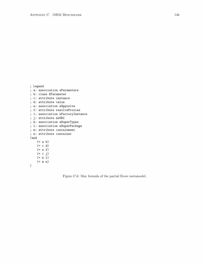
Appendix C. ORM Benchmark 146
; Legend
; a: association eParameters
; b: class EParameter
; c: attribute instance
; d: attribute value
; e: association eOpposite
; f: attribute resolveProxies
; i: association eFactoryInstance
; j: attribute nsURI
; k: association eSuperTypes
; l: association eSuperPackage
; m: attribute containment
; n: attribute container
(and
(= a b)
(= c d)
(= e f)
(= i j)
(= k l)
(= m n)
)
Figure C.6: May formula of the partial Ecore metamodel.

Appendix D
Supplementary Material to
Worked-Out Examples
In this appendix, we provide additional details about the worked examples in Chapter 8.
D.1 UMLet Bug #10
Figure D.1 shows the Mu-Mmint model K0 that encodes the UMLet model shown in Figure 8.1. The
encoded model contains the relevant slices of both the class diagram and the sequence diagram (bottom),
as well as traceability links between them, linking messages in the sequence diagram to operations in
the class diagram and objects to their classes. In the sequence diagram model, objects and lifelines are
represented by the same model element. Mu-Mmint uses yellow and pink stars to respectively indicate
edges that represent the source and target lifelines of messages.
Table D.1 shows the valid combinations of strategies for repairing the ClasslessInstance and Dan-
glingOperation consistency violations. Each combination represent a repair of the model shown in D.1,
i.e., a concretization of the partial model K1, shown in Figure D.2
Figure D.2 shows the diagram of the partial model K1 created by the maintainer to express her
uncertainty about which of the 44 alternative repairs in Table D.1 to select. To enhance diagram
readability, we have hidden the labels of the arrow model elements. This has resulted in hiding Maybe
annotations as well; however, it is easy to deduce that edges that are in K1 but not in K0 have Maybe
annotations.
Figure D.3 shows the ground propositional encoding φU1 of the property U1, expressed in SMT-
LIB [Barrett et al., 2010]. The formula encodes the property as a conjunction of the variables (cf.
atomToProposition) of the messages that are required to perform pasting.
Figure D.4 shows the ground propositional encoding in SMT-LIB of the sequence diagram well
formedness constraints for the slice of K1 involved in checking U1. Specifically, we check that for each
message in Figure D.3, there is an operation reference that maps it to the appropriate method definition.
The abbreviation “or” in the name of the variables means “operation reference”.
Figure D.5 shows the ground propositional encoding φU2 of the property U2 for K1, in SMT-LIB.
Specifically, we check whether the message setComponentZOrder exists in every concretization. We have
147

Appendix D. Supplementary Material to Worked-Out Examples 148
combined the property with the sequence diagram well-formedness constraint additionally requiring the
appropriate operation reference to the method definition.
Figure D.6 shows the model K2, a concretization of K1. It was created by invoking the operator
GenerateCounterExample with inputs K1 and U1. Mu-Mmint has greyed out Maybe elements of
K1 that are not also part of K2.
Figure D.7 shows the diagram of the partial model K3, resulting from invoking the operator Con-
strain with inputs K1 and U1. To enhance diagram readability, we have hidden the labels of edge
elements. Every edge that is outgoing from the elements new, moveToTop, setComponentZOrder, and
positioner is annotated with Maybe.
Figure D.8 shows the (concrete) model K4, resulting from invoking the operator Decide with K3 as
input while choosing the repairs RC4 and RD2.
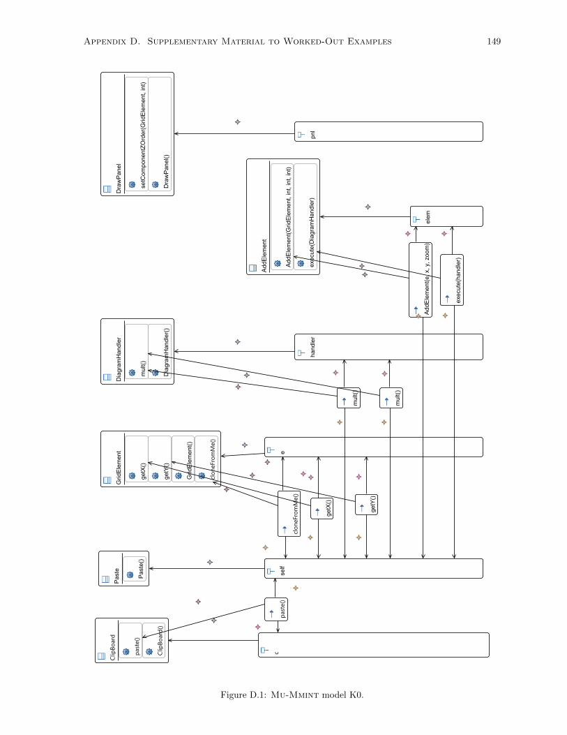
Appendix D. Supplementary Material to Worked-Out Examples 149
Figure D.1: Mu-Mmint model K0.
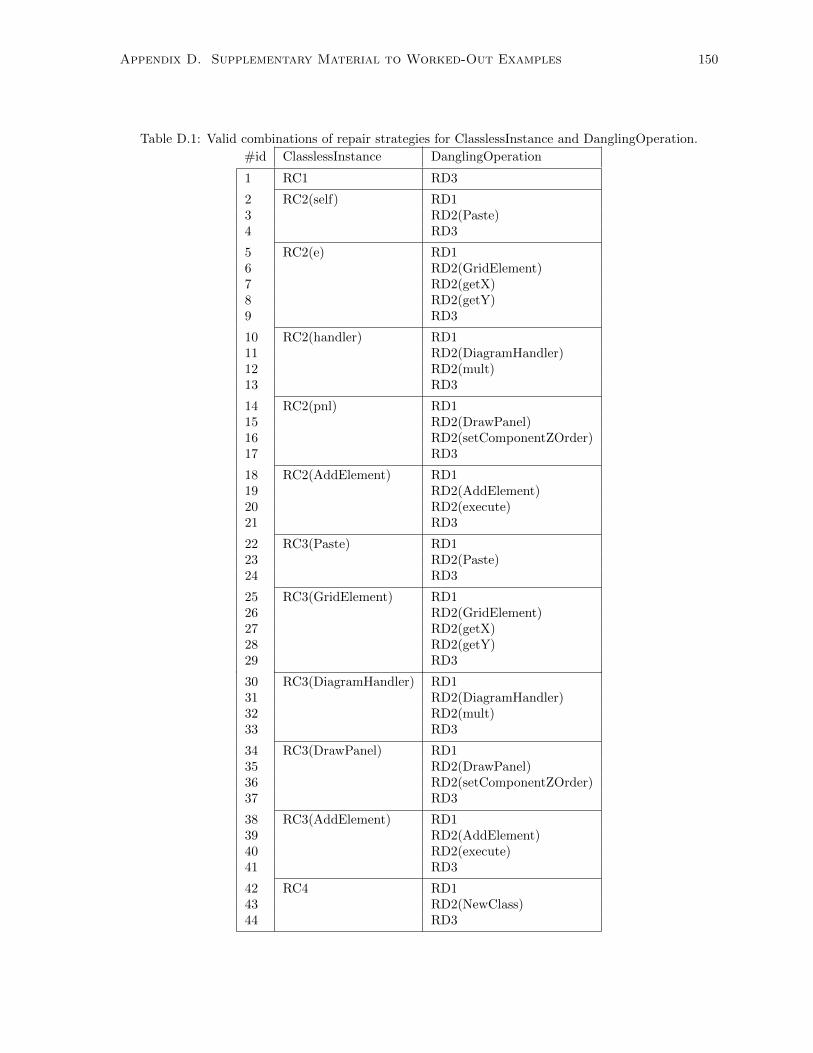
Appendix D. Supplementary Material to Worked-Out Examples 150
Table D.1: Valid combinations of repair strategies for ClasslessInstance and DanglingOperation.
#id ClasslessInstance DanglingOperation
1 RC1 RD3
2 RC2(self) RD13 RD2(Paste)4 RD3
5 RC2(e) RD16 RD2(GridElement)7 RD2(getX)8 RD2(getY)9 RD3
10 RC2(handler) RD111 RD2(DiagramHandler)12 RD2(mult)13 RD3
14 RC2(pnl) RD115 RD2(DrawPanel)16 RD2(setComponentZOrder)17 RD3
18 RC2(AddElement) RD119 RD2(AddElement)20 RD2(execute)21 RD3
22 RC3(Paste) RD123 RD2(Paste)24 RD3
25 RC3(GridElement) RD126 RD2(GridElement)27 RD2(getX)28 RD2(getY)29 RD3
30 RC3(DiagramHandler) RD131 RD2(DiagramHandler)32 RD2(mult)33 RD3
34 RC3(DrawPanel) RD135 RD2(DrawPanel)36 RD2(setComponentZOrder)37 RD3
38 RC3(AddElement) RD139 RD2(AddElement)40 RD2(execute)41 RD3
42 RC4 RD143 RD2(NewClass)44 RD3
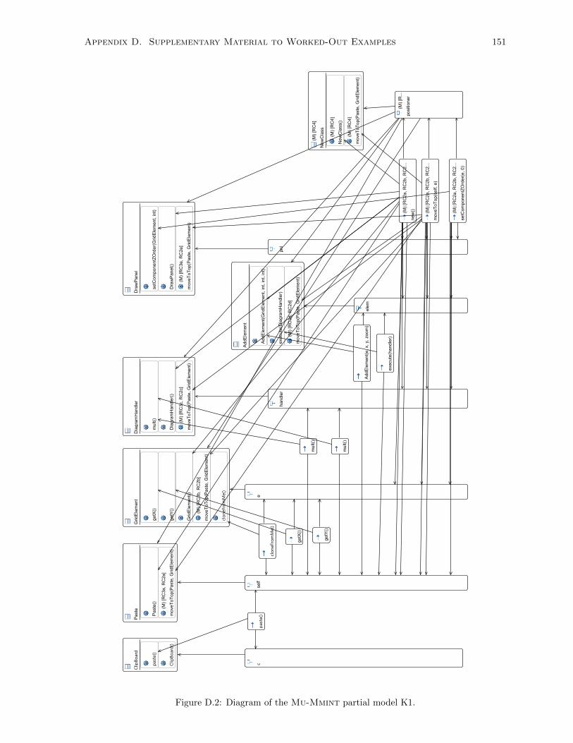
Appendix D. Supplementary Material to Worked-Out Examples 151
Figure D.2: Diagram of the Mu-Mmint partial model K1.

Appendix D. Supplementary Material to Worked-Out Examples 152
(and
(node paste_message)
(node cloneFromMe_message)
(node AddElement_message)
)
Figure D.3: Ground propositional encoding of the property U1.
(and
(edge or-paste-message2ClipBoard)
(edge or-cloneFromMe_message2cloneFromMe)
(edge or-AddElement_message2AddElement_constructor)
)
Figure D.4: Ground propositional encoding of sequence diagram well-formedness constraints involved inchecking the property U1.
(and
(node setComponentZOrder_message)
(edge or-setComponentZOrder_message2setComponentZOrder)
)
Figure D.5: Ground propositional encoding of the property U2.
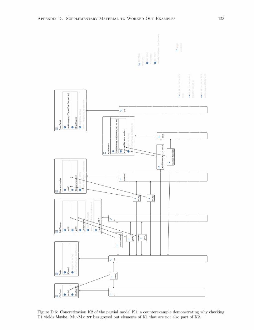
Appendix D. Supplementary Material to Worked-Out Examples 153
Figure D.6: Concretization K2 of the partial model K1, a counterexample demonstrating why checkingU1 yields Maybe. Mu-Mmint has greyed out elements of K1 that are not also part of K2.
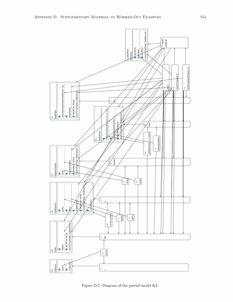
Appendix D. Supplementary Material to Worked-Out Examples 154
Figure D.7: Diagram of the partial model K3.

Appendix D. Supplementary Material to Worked-Out Examples 155
Figure D.8: Diagram of the final model K4, implementing the repairs RC4 and RD2.
Appendix D. Supplementary Material to Worked-Out Examples 156
D.2 Petri net metamodel
Figure D.9 shows the Mu-Mmint diagram of the partial metamodel N0. Meta-associations are decorated
with the icon “ ”, whereas containment references — with the icon “ ”. Maybe elements are annotated
with “[M]” and one or more alternatives from the uncertainty tree of N0 in square brackets. The
uncertainty tree of N0 is shown in Figure D.10.
The May formula of N0 is constructed from the uncertainty tree using the technique described in
Section 7.4. Specifically:
• The May formula is a conjunction of the decision variables:
d1 ArcClasses∧d4 Locations∧d5 TokenClass∧d7 Executions
• Each decision variable is equivalent to an exclusive disjunction of the alternative variables. For
example:
d1 ArcClasses⇔((d1ynw⊕
d1yw)⊕
d1n).
• Each alternative variable is equivalent to the conjunction of the Maybe elements that are anno-
tated with the alternative and the negations of the Maybe elements that are annotated with other
alternatives of the same decision. For example:
d1n⇔ src placeToTransition Association∧src transitionToPlace Association∧dst placeToTransition Association∧dst transitionToPlace Association∧¬ PlaceToTransition Class∧¬ TransitionToPlace Class∧ . . .∧ ¬ weight P2T Attribute∧¬ getWeight P2T Operation∧ ¬setWeight P2T Operation∧ . . .
With the exception of the class Location, the various meta-attributes, and the getter and setter
operators, the diagram of the metamodel N0 was created by merging slices of the AMZ metamodels
listed in Table 8.3. We sliced the AMZ metamodels in order to get a model that can be used with the
ORM transformation described in Appendix C, which requires the input class diagram to have a flat
class inheritance hierarchy.
Figure D.11 shows the ground propositional encoding φU3 of the property U3, expressed in SMT-
LIB [Barrett et al., 2010]. The formula encodes the property as a conjunction of the variables (cf.
atomToProposition) of the tables that are needed to map tuples from tables representing graphical PTN
elements to tuples of the table Location.
Figure D.12 shows the partial PTN metamodel N2 that results from invoking the operator Decide
on the partial model N0 to select the alternative d4y of the decision d4 Locations in the uncertainty
tree in Figure D.10.
Figure D.13 shows the diagram of the partial PTN metamodel N3 that results from invoking the
operator Expand on the partial model N2 to include uncertainty about which domain-specific PTN
constructs should be included in the ConcMod tool.
Figure D.15 shows the concrete PTN metamodel N5, resulting from invoking the operator Decide
with N3 as input and making the decisions d1yw, d2n, d3n, d5y, d6n, d7y, d8n, d9n, d10n from the
uncertainty tree in Figure D.14.

Appendix D. Supplementary Material to Worked-Out Examples 157
Figure D.9: Diagram of the partial metamodel N0.

Appendix D. Supplementary Material to Worked-Out Examples 158
d1 ArcClasses Are arcs represented as separate meta-classes?
[d1ynw] Yes. Arcs have weights.
[d1yw] Yes. Arcs do not have weights.
[d1n] No.
d4 Locations Is the location of elements in the diagram stored?
[d4y] Yes.
[d4n] No.
d5 TokenClass Is there a separate meta-class for tokens?
[d5y] Yes.
[d5n] No.
d7 Executions Is there a mechanism fore representing executions?
[d7y] Yes.
[d7n] No.
Figure D.10: Uncertainty tree of the partial metamodel N0.
(and
(node placeToLocation)
(node transitionToLocation)
(node tokenToLocation)
(node placeToTransitionArcToLocation)
(node TransitionToPlaceArcToLocation)
)
Figure D.11: Ground propositional encoding of the property U3.

Appendix D. Supplementary Material to Worked-Out Examples 159
d1 ArcClasses Are arcs represented as separate meta-classes?
[d1ynw] Yes. Arcs have weights.
[d1yw] Yes. Arcs do not have weights.
[d1n] No.
d5 TokenClass Is there a separate meta-class for tokens?
[d5y] Yes.
[d5n] No.
d7 Executions Is there a mechanism fore representing executions?
[d7y] Yes.
[d7n] No.
Figure D.12: Partial PTN metamodel N2.

Appendix D. Supplementary Material to Worked-Out Examples 160
Figure D.13: Partial PTN metamodel N3. The uncertainty tree is shown in Figure D.14.

Appendix D. Supplementary Material to Worked-Out Examples 161
d1 ArcClasses Are arcs represented as separate meta-classes?
[d1ynw] Yes. Arcs have weights.
[d1yw] Yes. Arcs do not have weights.
[d1n] No.
d2 ArcKinds Are there different kinds of arcs?
[d2y] Yes.
[d2n] No.
d3 Priority Do transitions have priority?
[d3y] Yes.
[d3n] No.
d5 TokenClass Is there a separate meta-class for tokens?
[d5y] Yes.
[d5n] No.
d6 Timed Are transitions timed?
[d6y] Yes.
[d6n] No.
d7 Executions Is there a mechanism fore representing executions?
[d7y] Yes.
[d7n] No.
d8 ColouredTokens Are tokens coloured?
[d8y] Yes.
[d8n] No.
d9 Stochastic Are transitions stochastic?
[d9y] Yes.
[d9n] No.
d10 Guards Are arcs guarded?
[d10y] Yes.
[d10n] No.
Figure D.14: Uncertainty tree of the partial metamodel N3.

Appendix D. Supplementary Material to Worked-Out Examples 162
Figure D.15: Diagram of the final PTN metamodel N5.

Index
Agile, 6
Aleatory uncertainty, 3
Applicability condition, 26
lifted, 68
Architectural layer, 29
Articulation stage, 84
operators, 87
Atom, 21
atomToProposition, 21
Backbone, 42
Base language, 35
Benchmark, 71
Bug #10, 102
CDO, 71
CIM, 29
Clafer, 47
Classical, 27
Cloning, 6
Computation Independent Model, 29
Concretization, 13, 32
Confluence, 28, 71
Consistent partial model, 32
Constrain operator, 90
Construct operator, 87
Correctness criterion, 66
Counterexample, 53
Databases, 61
Decide operator, 90
Deconstruct operator, 89
Deferral stage, 84
operators, 88
Degree of uncertainty, 32, 74
Design space exploration, 99
Diagnosis, 50
Diagnostic core, 54, 78
Donald Rumsfeld, 8
Drop operator, 75
Ecore, 71
Encapsulate Variable, 64
Epistemic uncertainty, 3
Equivalent partial model, 40
Expand operator, 87
F+ and F-, 52
Feature model, 47
FOL, 24
Forking, 6
GenerateCounterExample operator, 90
GenerateDiagnosticCore operator, 90
GenerateExample operator, 90
Graph, 20
Typed graph, 21
Graph rewriting, 25
Graph rewriting system, 27
Graph transformation, 25
Graph union, 23
Graphical Reduced Form, 42
Efficiency and sensitivity of construction, 78
graphToPropositionSet, 22
GRF, 42
Grounded formula, 24
Henshin, 10, 71
IDE, 96
Irreducible uncertainty, 3
Keep operator, 75
Known unknowns, 8
Lean, 6
163

INDEX 164
Left hand side, 25
LHS, 25
Lifted rule applicability, 68
Lifted rule application, 69
Lifting, 66
correctness criterion, 66
MakePartial operator, 87
Manual decision making, 75
Matching site, 25
MAVO, 47
May formula, 13, 32
Maybe elements, 13, 32
MDA, 28, 92
Megamodel, 81, 96
Metamodel, 20, 21, 45
constraining, 81
partialized, 36
reasoning, 60
MMINT, 71, 98
Model, 20, 21
Model Driven Architecture, 28, 92
Model management, 86
Model transformation, 25
MU-MMINT, 96
NAC, 25
Negative application condition, 25
Nondeterminism, 9, 46
Object-Relational Mapping, 71
OCL, 24
OMG, 28
ORM, 71
Partial behavioural model, 45
Partial behavioural models
reasoning, 60
Partial model, 32
consistent, 32
construction, 44
equivalent, 40
notation, 33
reduced form, 41
refinement, 33
semantics, 33
singleton, 32
transient, 86
Partialization, 36
Physics of Notations, 38
PIM, 29
Platform, 29
Platform Independent Model, 29
Platform Specific Model, 29
Presence conditions, 47
PRF, 43
Programming by Optimization, 6
Properties, 24
Property checking, 52
Property-driven refinement, 77
Propositional Reduced Form, 43
Provisionality, 6
PSM, 29
PtPP example, 1
Reduced form, 41
Reducible uncertainty, 3
Refinement, 33, 51, 75
property-driven, 77
Removal/addition of behaviour, 81
Resolution stage, 84
operators, 89
RHS, 25
Right hand side, 25
Rule, 25
applicability condition, 26
application, 25, 27
Lifted applicability, 68
Lifted application, 69
parts, 25
Scope, 7
scope, 46
Semantic properties, 24
Singleton partial model, 32
Software produce lines, 46
reasoning, 61
Software product lines
annotative, 47

INDEX 165
staged configuration, 81
SolvEx example, 63
Span, 7
span, 46
SPL, 46
Syntactic properties, 24
Teneo, 71
Termination, 28, 70
Traces, 51
Transform operator, 88
Transformation
application, 25
uncertainty-reducing, 76
Transformation rule, 25
Transient, 86
UMLet, 102
Uncertainty, 2
Aleatory, 3
degree, 74
Design-time uncertainty, 3
Environmental uncertainty, 3
Epistemic, 3
Irreducible, 3
propagation, 95
Reducible, 3
removal, 75
resolution, 75
Uncertainty management operator, 87
Uncertainty tree, 96
Uncertainty Waterfall, 83
extended, 85
operators, 87
transitions, 85
Underspecification, 9, 46
Unknown unknowns, 8
URT, 76
Variability, 47
management, 100
reasoning, 61
variability-aware techniques, 61
Verification, 24, 50
feasibility, 55
scalability, 55
semantics, 51
Verify operator, 88
Waterfall model, 85
Well-formedness constraints, 21
WFC, 21