•

•

IvODELING FOREST SUCCESSION

by

Samuel J. Harbo, Jr.

Institute of Statisticsl~meographed Series No. 844September 1972

•ABSTRACT

HARBO, SAMUEL JAMES, JR. Modeling Forest Succession. (Under the

direction of ARTHUR WELLS COOPER and DON WILLIAM HAYNE).

A simulation model is developed to aid in explaining the processes

involved in forest succession. The model requires information of

species changes at randomly located points and the probability of

such changes. Covering of a point by a plant's aerial parts is the

characteristic used in determining state. A full, or unsimplified,

model is specified first, but due to the complexity of succession

and hence of the full model, various simplifications are specified.

In the simplified reduced "model, plant states at a point are

specified on an age-group basis, with each age group having an

associated transition matrix whose entries are the probabilities of

state changes for plants of that age group to the next older age

group. Feedback relationships portraying interactions between

species, as well as between age gr6ups, are specified in the model.

A seed vector containing the probabilities of a point being covered

by a species' seed also is specified. The model is programmed for

a digital computer.

Five simulated successions illustrate some uses of the model.

The rationale followed in determining which simplifications

should be used in reducing the complexity of a model and the model­

field study interactions are discussed.

• MODELING FOREST SUCCESSION

by

SAMUEL JAMES HARBO, JR.

A thesis submitted to the Graduate Faculty ofNorth Carolina State University at Raleigh

in partial fulfillment of therequirements for the Degree of

Doctor of Philosophy

DEPARTMENT OF EXPERIMENTAL STATISTICSDEPARTMENT OF BOTANY

RALEIGH

1 9 7 2

APPROVED BY:

Co-Chairman of Advisory Committee Co-Chairman of Advisory Committee

•

..

ii

BIOGRAPHY

I was born on March 3, 1929, at Hanska, Minnesota. I was reared

at that locality and received my first 12 years of formal education

there. I attended the University of Nebraska, receiving a Batchelor

of Science Degree in Soil Conservation in July, 1951.

After serving three years in the United States Navy, I enrolled

at the University of California, Berkeley, spending three semesters

there. I then enrolled at the University of Alaska, receiving a

Master of Science Degree in Wildlife Management from that institution

in 1958.

I was employed as a wildlife biologist by the Alaska Department

of Fish and Game from 1958 to August, 1961. At that time I entered

graduate study at North Carolina State University. During the

periods August, 1961 to July, 1964 and June, 1966 to July, 1967 I was

in residence at North Carolina State University completing the course

requirements for my doctoral program.

In September, 1964 I accepted a teaching position at the

University of Alaska; I am currently employed there.

I marri.ed Gayle Whitten on May 1, 1958. We have four children;

Li.sa Ann, 12 years; Lora Kay, 10 years; Keith William, 7 years; and

Sam Jens, 4 years.

•

...

iii

ACKNOWLEDGMENTS

I wish to express my appreciation to the co~chai:rmen of my

advisory committee J Professors A. W. Cooper and D. W. Hayne, for

their advice and guidance. I also wish to thank the other members

of the committeeJ Professors II. L. Lucas J C. Proctor and

H. R. van der Vaart J for their constructive criticisms.

I am grateful for the financial support I received during my

doctoral study. I held a Research Assistantship with the

Cooperative Wildlife Statistics Project for one year and a National

Institute of Health Fellowship through the Biomathematics Program

for three years.

I also wish to express special gratitude to my w:Lfe; Gayle; and

my children for their patience, sacrifice and encouragement during

the course of my study•

•iv

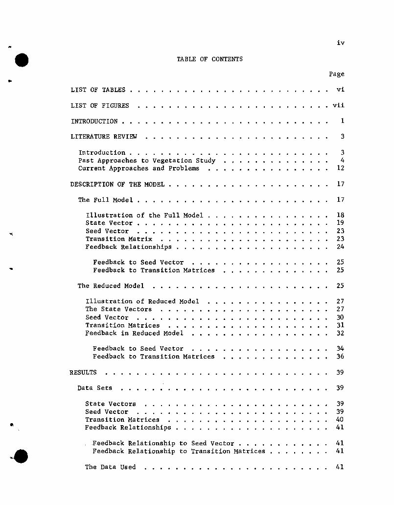
TABLE OF CONTENTS

Page

LIST OF TABLES •

LIST OF FIGURES

INTRODUCTION • •

LITERATURE REVIEW

Introduction. . • . • • .Past Approaches to Vegetation StudyCurrent Approaches and Problems

DESCRIPTION OF THE MODEL

The Full Model

Illustration of the Full Model .State Vector • . . .Seed Vector • • • • •Transition MatrixFeedback Relationships • .

vi

. . vii

1

3

34

12

17

17

1819232324

•Feedback to Seed VectorFeedback to Transition Matrices

The Reduced Model

. . . .. .2525

25

..

Illustration of Reduced Model • . . . •The State Vectors . • . • •Seed Vector . • • . . • . .Transition Matrices . . • • • •Feedback in Reduced Model

Feedback to Seed VectorFeedback to Transition Matrices

RESULTS

Data Sets

State Vectors • •Seed VectorTransition Matrices . . • .Feedback Relationships .

Feedback Relationship to Seed Vector . . • • •Feedback Relationship to Transition Matrices .

The Data Used

2727303132

3436

39

39

39394041

4141

41

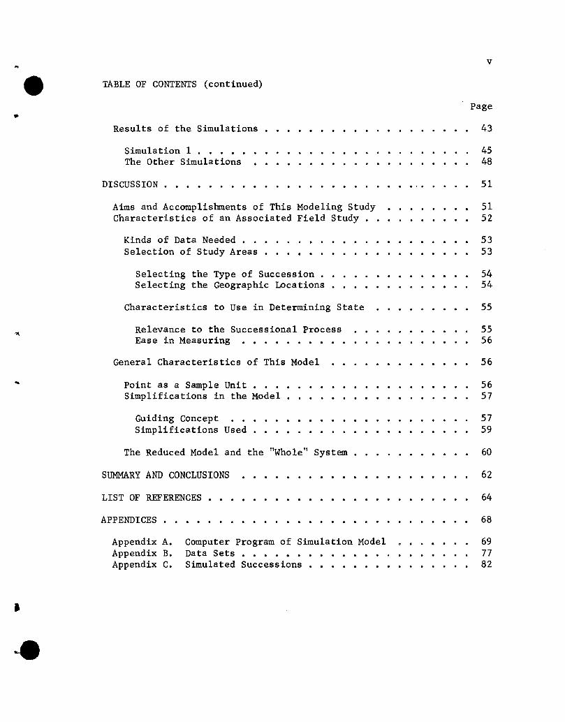
•• TABLE OF CONTENTS (continued)

Results of the Simulations •

Simulation 1 . . • • • •The Other Simulations • . . •

DISCUSSION • • • • • • • •

Aims and Accomplishments of This Modeling StudyCharacteristics of an Associated Field Study •

Kinds of Data Needed • . •Selection of Study Areas •

Selecting the Type of SuccessionSelecting the Geographic Locations •.

Characteristics to Use in Determining State

Relevance to the Successional ProcessEase in Measuring . • • • • • • •

v

Page

43

4548

51

· · · · 51

· · · · 52

5353

· · · · 54. . · · 54

55

5556

..General Characteristics of This Model

Point as a Sample Unit • . • • .Simplifications in the Model •

Guiding ConceptSimplifications Used

The Reduced Model and the "Whole" System •

SUMMARY AND CONCLUSIONS

56

5657

5759

60

62

LIST OF REFERENCES •

J

APPENDICES

Appendix A.Appendix B.Appendix C.

Computer Program of Simulation ModelData Sets • • • • • •Simulated Successions • • . • • • • •

· · · · 64

68

69. · · · · 77

· · · · 82

•..

..

1.

2.

LIST OF TABLES

The probabilities that a seed will cover a randomlyselected point given four seed production rates andtwo seed sizes . . . . . . .. .".... a ••

The INTER and RESEED matrices in the five data setsused in this study • • . • • • • • • . .

vi

Page

40

42

•1.

2.

LIST OF FIGURES

A possible sequence of events at one specific pointduring a five-year interval of a forest successioninvolving only 2 species, A and B, and 6 age classes

A diagram showing the changes from year t to year t+1as two-year-01d plants of species A and B mature tothree-year-01d plants •• . • • • . • • . • • •

vii

Page

20

28

3. The probabilities, reflecting per centone-year-01d plants generated from aseed probabilities and from a matrixprobabilities • • • • • • • . • • •

cover, forvector containingof transition

33

• INTRODUCTION

Vegetation is a dynamic phenomenon, yet many investigators have

tended to treat it as though it were static. Numerous treatises have

dealt with spatially-related change and variability in vegetation,

and the methodologies to measure, reduce or remove that change or

variability. Numerous workers, concerned with vegetation modifica­

tion with time, have recorded time-related vegetation changes, but

they also have collected the data as though vegetation were static.

Methodologies, both collecting and analytic, have not been developed

to handle the dynamic aspect. Partly as a consequence, the roles of

the processes involved in the principal dynamic aspect of vegetation,

succession, are not well understood, even though succession has been

an important topic in ecology for over half a century. Some of the

deficiencies in our understanding undoubtedly also reflect the

complexity of plant succession, and I believe some also reflect the

orientation of many succession studies. F. C. Clements' overwhelming

influence on ecological perspective in the early 1900's, and to some

extent even today, stimulated many studies devoted to chronicling the

products of succeSSion, and presumably the invariance of the climax

vegetation, but not the processes themselves.

The complexity of natural phenomena usually is of sufficient

magnitude so that field studies conducted without supporting experi=

mental and theoretical investigations are incapable of explaining, in

a causal relationship context, the phenomena. That assertion

particularly applies to vegetation, and to vegetation study. An

additional complication usually associated with vegetation study is

..

••

2

the length of time required for completion of vegetation processes,

and the subsequent manifestation of change. A hundred years or more

may be required before a relatively unchanging forest stand re­

occupies an abandoned field, for example. Since man's impatience

and urgency demand answers now, not 100 years from now, telescoping

of the time span i.s essential.

The present study, considering vegetation is a dynamic phenomenon,

attempts to evaluate the roles played in vegetation development by

the various processes involved in succession. I attempt to develop

a model that is complementary to an associated field study and which

will provide a means for collecting the information needed to resolve

such questions as the role of chance, competition and other factors

in determining plant groupings. The model is designed with special

reference to forest succession and is structured to aid in telescoping

of the time span.

..

•..

..

3

LITERATURE REVIEW

Introduction

The stimulus for community ecology and succession study largely

is due to three men, Frederic Clements, Henry Cowles and Eugene

Warming. Their works stressed the concepts of community and plant

succession.

Warming (1909), and many earlier workers, recognized that

species are not randomly distributed but form associations of varied

physiognomy. Warming believed that the study of associations involved

determining which species associate together, why they associate, why

the associations have a characteristic physiognomy, why each species

has its own special "habit and habitat," and the means plants employ in

order to live in a given environment. These points of inquiry still

are current.

Cowles (1899) studied the succession of sand dune vegetation

near Lake Michigan. He believed that vegetation was the joint product

of past and present environments, and to understand the development

of vegetation, succession must be studied. Such studies should attempt

to discover the "laws" governing vegetation changes.

Clements (1916) accepted the community not only conceptually but

factually. He believed in the importance and near organismic equiva­

lence of communities, which prompted the questions of how communities

arose, why some were replaced by others and why some seemed to persist

indefinitely. To Clements, communities, and not individual species,

are the important elements in succession, because the motive force

in succession lies in the responses or functions of groups of

•4

individuals. These responses or functions, producing different

moisture regimes or soil structure, or other habitat reactions,

depend on the life form of the group. A life form able to produce

reactions causing stabilization received Clements' term dominance,;

plants of that life form were termed dominants. The concept of

dominance and dominants is a focal point in Clements' vi.ew of

succession.

Clements (1928) also considered competition an important factor

in succession. He indicated that competition occurs only when plants

are more or less equal; a dominant tree-understory herb relationship

is not one of competition but is one of dominance and subordination.

A tree seedling and herb could compete, however. Also, the dominants

influence the competitive balance of the understory by modifying the

environment. Although competition contributes to a community's reac­

tion upon its habitat, Clements believed that dominance was of much

greater importance.

Past Approaches to Vegetation Study

Clements strongly influenced the direction of vegetation study in

North America during the first half of the 20th century. He stressed

the regularity and directional aspect of succession and the ultimate

invariance and importance of the terminal stage, labeled the climax

community. Clements' emphasis of the units of vegetation and of

successional invariance caused many of the North American pl.ant

ecologists to focus their attention on community cl.assification and

on detailing community sequences in succession.

•

..

•.5

Concurrent with the development of the climax concept, various

other ecological schools or traditions developed. Most were

classificatory in nature (Whittaker, 1962), and most accepted explic­

itly or implicitly a "natural" unit of vegetation (McIntosh, 1967).

This belief in "natural" and floristi.cally homogeneous units of

vegetation influenced the sampling and analytic methodology used in

vegetation study. In one widely-accepted approach to vegetation

study, the Braun-B1anquet approach (Braun-Blanquet and Furrer, 1913;

Braun-B1anquet, 1932), such methodology is an important and integral

aspect of the approach. The approaches based on the objective

reality of vegetation units gradually became known as the community­

type approach to vegetation study (McIntosh, 1967).

Not all workers believed in the invariance of succession or the

objective reality of plant communities, however one, H. A. Gleason,

conceding that units of vegetation exist (Gleason, 1917) although they

may be only coincidences (Gleason, 1926), stressed that the develop­

ment and maintenance of vegetation results from the development and

maintenance of the component individuals. Gleason reasoned that

plant composition is determined by environmental sorting of i.mmigrants

from surrounding areas, and inasmuch as adjacent areas possess similar

environments and receive immigrants from the same or very similar

plant populations, areas of similar, but not precisely the same,

vegetation should result. Gleason recognized that dense vegetation

can modify and control the environment and consequently species

composition and abundance, but he reasserts that the establishment or

non-establishment of a plant on an area is determined by the arrival

••

•

6

or non-arrival of a propagu1e and by the environment encountered, and

not by the vegetation per~. The result, according to Gleason, is

that these two primary causes determine the plant life on every

"minimum area," and as a consequence large areas of very similar

vegetation do not occur. This concept of plant associ.ation Gleason

termed the individualistic concept.

Concurrent with development of the i.ndividua1i.stic concept,

a Russian, L. G. Ramensky (1926), independently developed a similar

philosophy regarding plant groupings. Ramensky shared Gleason's

belief in the ecological individuality of each speci.es, and that each

plant reacts individually to the environment it encounters. Ramensky

emphasized that plant cover changes continuously in space and that

sharp boundaries between locally homogeneous plant groupings are

exceptional, requi.ring special explanation such as hum.an inter­

ference, discontinuous alteration of other factors, etc.

Gleason's and Ramensky's concepts of vegetation received little

support until Stanley Cain's paper appeared in 1947 (Cain, 1947).

Cain argued that each species in a vegetation stand has its individual

area of occurrence and a more or less unique ecological amplitude

and modality. Consequently, a floristic natural area occurs if the

limits of areas of occurrence of a large number of species fall in the

same place. In essence, a floristic natural area is characterized

by the exclusiveness of a number of plants. As a consequence,

associations are local phenomena and are i.ndividualistic because they

cannot be more extensive than the superposition of areas of the

species involved.

•

••

•

7

Curtis and McIntosh (1951), working in the prairie-forest

floristic province of Wisconsin, also attacked the question of the

objective reality of a plant community. They stipulated that only

within floristic provinces, which have uniform flora and are similar

to Cain's natural areas, can plant associations possibly achieve

objective reality. The two investigators studied relatively natural,

undisturbed stands of deciduous forests growing on upland forms in

southern Wisconsin, deleting from study heterogeneous stands but

accepting homogeneous ones regardless of their species composition.

The two workers attempted to classify the stands into groups, using

an index termed importance value. Several orderings, based on

different assemblages of species, were tried. No discrete grouping

of species was apparent; rather, the entire collection of species

formed a continuum. Curtis and McIntosh conclude that their findings

substantiate Gleason's individualistic association hypothesis, but

with the restriction that the available flora's physiological

potentialities and the existing environment limit the species combina­

tions that can occur.

Whittaker (1956), working in the Great Smoky Mountains concurrent

with, but independent of, the work in Wisconsin, sampled the vegeta­

tion without regard to apparent plant associations. The findings were

related to known environmental gradients, using an analytic technique

that Whittaker termed direct gradient analysis. Whittaker reasoned

that the existence of valid vegetation types, and their relationship

fo environmental gradients, would be revealed by abrupt changes in

species composition and distinct groupings of species' maximum points,

••

•

•

8

when various plant characteristics were plotted on environmental

gradients. Abrupt changes and distinct groupings did not occur;

Whittaker concluded that species are not organized into distinct units

but that stands and vegetative types are mainly continuous with one

another. Although using different sampling and analytic techniques,

Whittaker's conclusions support those of Curtis and McIntosh.

The studies by Cain, Curtis and McIntosh, and Whittaker changes

the perspective of ecological thought in North America, causing re­

evaluation of Clements' climax-oriented approach and provoking re­

appraisal of Gleason's individualistic concept. The organismic

equivalence and invariance of a community were placed in doubt, and

the regularity of the successional process was questioned.

Numerous studies concerning succession have appeared since

Gleason's advancement of the indiVidualistic hypothesis. Some

studies, such as Wells' (1928) study of the successional relation­

ships of plant communities on the North Carolina coastal plain,

considered communities as concrete entities; but other studies were

less community-oriented and more autecological in nature (dePeralta,

1935; Pessin, 1939; Baldwin, 1940). A broader approach to succession­

al studies appeared, however. Billings (1938), for example, explained

old-field succession of woody species in terms of interspecific

competition, individual species competition and species-induced

environmental changes.

Keever (1950) studied the herbaceous vegetation that precedes

the woody in old-field succession and found that competition, plant­

induced environmental changes and timing of the life cycles

•

•

•

•

•9

significantly influenced succession. She also observed that a

species can modify the environment in a way detrimental to its own

survival and that insufficient seeding rates can delay a species'

attainment of dominance. Many other workers also have recognized

the importance of seeding rates, and numerous studies have dealt with

the variability in seed production and the factors influencing seeding

rates and seed germination (Bormann, 1953j McVean, 1953j B1ack~ 1958j

Allen and Trousde11, 1961j Shoulders, 1961; Harper and McNaughton,

1962j phares and Rogers, 1962j Stephenson, 1963).

The conflicting views regarding vegetation have resulted in two

distinct trends in the approach to vegetation interpretation. The

first trend, probably arising with the advent of scientific interest

in vegetation, treats vegetation as composed of "well-defined,

discrete, integrated units" (McIntosh, 1967). This trend is called

the community-type concept. The second trend, termed continuum

concept, holds that vegetation changes continuously and is not dif­

ferentiated, except arbitrarily, into sociological entities (McIntosh,

1967). Although considered a linear descendent of the individualistic

hypothesis, the continuum concept originated in the works of Curtis

and McIntosh (1951) and Whittaker (1956). These two trends have

created a community-contiuuum controversy that has influenced vegeta­

tion study. A discussion of some points of controversy and their

influence on vegetation study follows.

Some investigators apparently interpret their findings in a

manner consistent with their view of vegetation. Poore (1956), for

example, specifies that a plant community should be described

•

•

•10

according to its present characteristics rather than according "to

what it has been or what it is thought about to become." Daubenmire

(1966), on the other hand, stresses the need to consider stability

when studying vegetation. He reconunends that only areas of "maximum

homogeneity" be sampled, and preferably only climaxes, or potential

climaxes "n areas judged to have preclimax vegetation, be considered.

Monk (1968) succinctly illustrates the vegetation concept-

interpretation interaction by stating (p. 303),

..

•

That earth is continuously covered by vegetation isprobably the only fact all vegetation analysts wouldaccept. • .• It would be safe to say that if tworesearchers of the vegetation continUity-discontinuityschools were permitted to examine the same 1000"conununity stands" the resultant would be a continuumon the one hand and a conununity-type classification onthe other. One side would argue that the subjectivesample selection is an end in itself whereas the otherwould propose methodology, state of successi,on, etc.

Leith (1968) claims that the goals of the two concepts are

different: the goal of the conununity-type approach is a vegetation

map while the goal of the continuum approach is the "key-lock

explanation of each single species demand on the environment."

Leith finds nothing wrong with either approach, except when

pertinent information is ignored: for example, when continuum

advocates deny the existence of characteristic species and the

conununity-type advocates ignore overlaps. Monk (1968) claims that

the conununity-type adherents minimize and the continuum advocates

maximize the importance of the transition zones. Both Monk and

Leith agree that in unraveling the causal relationships between

vegetation and environment, the continuum approach seems most

promising.

•

•

..

•11

An investigator's concept of vegetation influences the

methodology he selects (Yarranton, 1967a). A basic aspect, selection

of study areas, is influenced. Community-type adherents tradition­

ally have used subjective selection (McIntosh, 1967); they claim it

is a major advantage of their approach (Becking, 1957; Poore, 1956

and 1962). Daubenmire (1966) believes that the areas must be sub­

jectively sampled to insure "maximum homogeneity" or the samples will

be virtually worthless. Continuum advocates reject that contention,

arguing that areas must be objectively chosen, at least for some

broadly defined vegetation type, so that preconceived ideas regarding

the vegetation do not influence the selection process (Cottam and

Curtis, 1949; Curtis and McIntosh, 1951; Whittaker, 1952 and 1962;

Goodall, 1963). Cottam and McIntosh (1966) cite the need to sample

the majority of ari area '.8.' vegetation, and not only those parts that

are amenable to grouping into discrete associations. Some investi­

gators question whether sampling, and in particular random sampling,

of vegetation is possible or useful. Egler (1968) infers that sampling

is questionable if stands of vegetation are "coincidental phenomena,

with each stand having the chance possibility of being 'significantly'

different from the others." Major (1958) argues that sampling can

be carried out only within a defined population. Therefore, defining

qualitatively homogeneous populations is a prelude to sampling. Major

believes that vegetation is not a random chaotic assemblage of plants

but is ordered. He concludes that random sampling of all of an area's

vegetation would be useless.

•

•

..

.. 12

Current Approaches and Problems

The continuing community-continuum controversy has accentuated

the need to critically evaluate the kinds of vegetation information

collected and the methodologies required for their collection.

Harper (1967) notes that measures of population turnover are com­

pletely obscured by methodologies used in most vegetational studies.

Only if individual plants are marked and repeatedly observed can

population turnover be assessed. Harper conjectures that plant

species plasticity and the ability to reproduce vegetatively are the

two main reasons why plant ecologists have not stressed numbers.

Yarranton (1966), concerned with vegetation variation and the

sampling methods required for its elucidation, postulates that varia­

tion is determined by the distributional patterns of species compris­

ing the vegetation. These patterns can be analyzed in physical terms

in real space, or by "abstract statements" of plant interrelation­

ships that may be explicable in terms of real space. Plot sampling

methods are suitable for the former, Yarranton claims, but plotless

methods are required for the latter.

An analysis of each species' distribution with respect to

environmental variables and other species is required for evaluating

the individualistic hypothesis (Yarranton, 1967b). Time is an

important factor requiring incorporation in the analytic scheme

(Yarranton, 1967bj Becking, 1968). Becking, stressing the need to

consider the dynamic aspect of vegetation, cautions that the time

scale used in a study can influence an investigator's perspective.

Becking believes that community descriptions are only relevant as

momentary time-lapse pictures of the ever-changing community.

•

•

•

•

•13

The degree of integration or organization in a plant community

is an important consideration in vegetation study. Two of the early

workers, Clements and Gleason, differed greatly in their views of

integration; Clements believed communities possessed a high degree

of integration, but Gleason felt it was inconsequential. The dif­

ference in emphasis still persists among current investigators.

Poore (1964), analyzing the evidence supporting integration, indi­

cates that two factors, opportunity and competition, determine the

composition of a community. Opportunity determines the species

composition of the propagules reaching the area, and competition

sifts out those species that will persist in the environment

encountered. This sifting and selection, acoording to Poore,

establishes a dynamic balance in the community that is reflected in

community structure and pattern. This structuring, and possibly other

manifestations of competition, lends inertia to the community and

tends to inhibit community change. Poore believes that to understand

natural vegetation we must understand integration's role. Detailed

studies of the autecology of species under competitive conditions of

natural communities are needed. Poore suggests that integration

should be an essential part of the definition of community.

Understanding the selective processes operative during develop­

ment of a community is essential in order to understand the nature

of vegetation structure (Anderson, 1965). Knowing the quantitative

and qualitative importance of both the intensity and duration of

selection is required. Anderson postulates that the ultimate

structure of vegetation depends upon the parts played by chance and

•..

•

~.

14

selection; if selection is weak and intermittent, chance plays a

substantial role. But, if selection is intense and persistent,

chance contributes only slightly. Based on a study in northwest

Iceland, Anderson et a1. (1966) concluded that intense selection

exerted by the "harsh" environment limited the number of successful

species; a weakly developed, climatically controlled continuum

resulted. Poore (1967) suggests that opportunity and selection

operate differentially on different segments of a vegetation's flora.

He contends that the occurrence of the less common tree species in

a tropical forest is correlated with physical environmental factors,

which implies that selection has influenced the distribution of those

species. The more common species, however, appear to be influenced

less by environmental factors than by chance of dispersal and

establishment. Not all workers agree with Poore's interpretation,

however (Austin and Greig-Smith, 1968).

The complexity of vegetation undoubtedly is causing ecologists

to seek special tools and techniques. Austin and Greig-Smith (1968)

indicate as much when they criticize Whittaker's (1967) assertion

that the simpler ordination techniques are more likely to provide

advances in ecological understanding than are the more elaborate

techniques. Slobodkin (1965) stresses the point that field studies

cannot stand alone, stating (p. 349),

. • it is almost certain at the moment that fieldobservation by itself, in the absence of laboratoryand theoretical study, is almost useless in providingexplanations (of field phenomena) •.. theoretical andlaboratory analyses can provide limits for the possiblefunctions of various processes in the field . . • makingpossible, decisions between various alternativehypotheses with respect to field data.

•...

•

~.

15

Quantitative analytic techniques are increasing in importance

in vegetative study. Goodall (1963), for example, used geometric

models based on vegetation space having an axis for each species

comprising the vegetation and plotting each sample area as a point in

that space. He stressed that the distribution of points in vegeta­

tion space reflects two completely distinct factors: 1) the frequency

distribution of the different sites, and 2) the "adaptations" of

species locally available to the ecotope and to each other. Goodall

observes that if clumping of points depends only on unequal avail­

ability of sites, the clusters of points do not reflect different

communities, or at least not well-integrated communities. If the

points show clumping, while the distribution of sites does not,

strong "presumptive evidence" for an integrated community exists.

Modeling also is increasing in importance. Two modeling

approaches particularly pertinent to vegetation study are advanced

by Leak (1968) and Yarranton (1969). Leak formulates a probability

model to depict birch regeneration in a clear-cut area. The model,

essentially a branching diagram of probabilities, considers prob­

abilities for events ranging from development of a female flower to

the growth of a commercially acceptable stem. The model, although

rather specific, is a valuable contribution to vegetation study, for

it demonstrates that variables such as conditional probabilities can

furnish insight into vegetation processes.

A different approach to modeling is advanced by Yarranton.

Using point sampling procedures, Yarranton uses a species' presence

or absence at a defined point as the characteristic of interest.

•

•

~.

16

That characteristic serves as the dependent variable and is combined

with independent variables such as the presence of plants of the

same or other species at various distances from the defined point,

environmental factors and time, in a regression analysis. Yarranton

acknowledges that application of the model to natural succession may

prove difficult, particularly because of the number and difficulty of

measurement of possibly pertinent independent variables. Initial

application perhaps should be too simple, controlled growth studies,

but Yarranton obviously believes the models' main potential is for

broad application. He states (p. 249),

The model described above provides a basis forcomparative studies of the ecology of single speciesand of the interaction between them, and is unifyingin the sense that the results of many types of ecologi­cal investigation, including pattern analysis, inter­specific association and auteco1ogica1 experiments, canall be incorporated. It also provides the theoreticalbasis for a new approach which may lead to quantitativeanalysis of succession.

The latter aspect, the new approach to succession studies, may be the

most significant aspect of Yarranton's modeling work.

••

•

..

17

DESCRIPTION OF THE MODEL

The model for succession proposed here will be stated first in

its full form, but then of necessity it will be modified to a form

that is feasible in the present states of knowledge and computer

capability.

The Full Model

Succession is defined with reference to points on the earth's

surface, as the present state along with the set of probabilities of

state transition during the next time interval. By the state at a

point is meant the species and age composition of plants covering the

point; thus there are many possible states. The probabilities refer

to transition from the present state to anyone of all the possible

states, including the present state. Vegetational succession is thus

identified as a non-random change in time of the distribution of

states for the set of all points on the surface.

There are three principal elements of this model of succession.

These are the vector of all possible states, the matrix of transition

probabilities for the next unit of time, and a feedback mechanism.

The feedback permits environmental factors to modify the transition

probabilities and also to alter the seed vector which is a special

subset of the state vector.

The model can be written as:

s e s~t+1 = ':( t, t; 1)-t

••

•

18

where

s-t = state vector at time, t

!t+l = state vector at time, t+l

e-t = vector of environmental forces at time, t

T = transition matrix whose elements are functions

of !t' !t' and ~

e = vector of parameters involved in T.

The number of elements in s will be very large if the model is

to be realistic. The functional form of T, in order to be realistic,

will also be very complex.

The composition of the parameter vector, !, will depend on the

functions specified for the elements in T. The elements in e will

include plant parameters such as growth rates, but they also might

include those relatively unchanging environmental factors that are

not plant modified.

Illustration of the Full Model

The forest succession model I propose may be identified with

secondary succession on a recently denuded forested area. I assume

that woody species immediately invade the area; the model applies

to vegetational development and change at points located on the

denuded area. The model involved defines the presence of plants,

the states, at the pOints, and the probabilities that the situation

will persist or change during the next time interval.

••

•

19

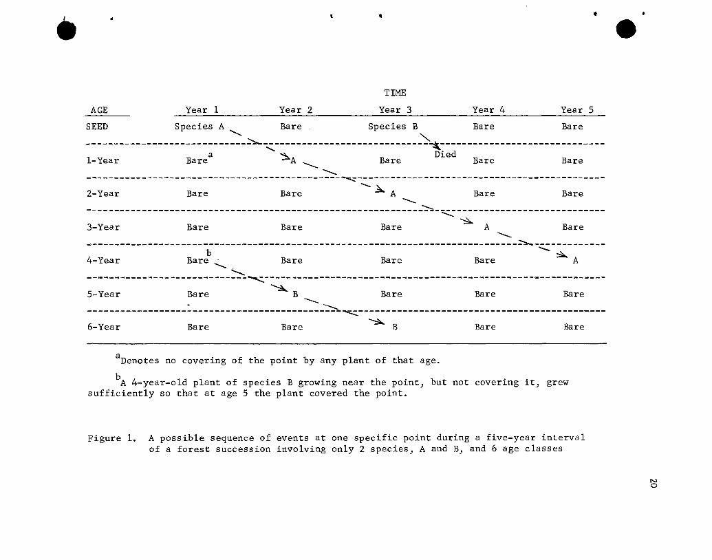
This general approach can be illustrated by a possible sequence

that could occur at a point during a very simple succession. In

Figure 1, I have listed a possible five-year sequence for a succession

involving only 2 species, A and B. During year 1 of the sequence,

a seed of species A falls on the point. That seed germinates and

survives, so that at year 2, a year-old plant of species A covers the

point. That plant persists throughout the five-year sequence, re­

corded as a successively older species A plant during each of the

last three years.

A species B plant, five years old, covers the point at year 2,

although it was not recorded at the point in year 1. Such an

occurrence may result if a 4-year-old plant growing near the point,

but not covering it, grows sufficiently during year 1 so that by

year 2 the 5-year-old plant covers the point. Species B also is

represented in the 5-year span by a seed that appears at year 3 but

does not produce a viable 2-year-old plant.

State Vector

The elements of the state vector are defined to be the fractions

of the points on the area covered by all possible combinations of

species and age classes, as well as by bare ground. The different

ways of coverage could be, for example, coverage by, but only by:

bare groundj one individual of a given species of a given agej two

individuals of a given species of a given agej three individuals,

etc.j two individuals of different species of the same age, etc.j

two individuals of a given species of different agesj two individuals

of different species and different agesj three individuals of different

•AGE

-.

Year 1 Year 2

•

TIME

Year 3 Year 4

t

Year 5

•SEED Species A Bare Species B Bare Bare

......... "-----------------------------~------------------------------~------------------------------a ' ~ Died

l-Year Bare ~A "- Bare Bare Bare------------------------------------------------~------- --------------------------------------

2-Year Bare Bare ......... ~ A Bare Bare............

------------------------------------------------------ -------~-------------------------------"--.~

3-Year Bare Bare Bare A Bare-------------------------------------------------------- ------------------------~-------------b "--.~

4-Year Bare '-- "'- Bare Bare Bare A

-----------------------------~--------------------------------------------------------------

~5-Year Bare B Bare Bare Bare--. ------------------------------------------------~------- --------------------------------------

~6-Year Bare Bare B Bare Bare

aDenotes no covering of the point by any plant of that age.

bA 4=year-old plant of species B growing near the point, but not covering it, grewsufficiently so that at age 5 the plant covered the point.

Figure 1. A possible sequence of events at one specific point during a five-year intervalof a forest succession involving only 2 species, A and B, and 6 age classes

No

•

..

..

..

21

species and different agesj etc.j through all possible combinations

of coverage by different numbers of individuals of different species

of different ages. The model reflects a composite of all states

at all points.

This set theoretic description of successional state has

three immediate advantages. First, it conforms to the widespread

use of cover as a field measurement in plant ecology. Second, it

permits the direct field estimation of state by sampling of randomly

selected points. Third, it provides the logical basis for a

description of change and permits a rigorous definition of the

dynamic process of succession.

Plant ecologists have used characteristics other than cover

to describe vegetational state by field sampling. Density,

frequency, abundance and basal area, in addition to cover have

received greatest use. The first three are popu1atio~not individ­

ual plant characteristics, and thus are not suitable for specifying

the states at sample points. Basal area is an individual plant

characteristic, but in order to use it for describing states at a

point additional specifications are necessary. For example,

is the basal area use d for the plant whose stem covers the

point, for the stem nearest the point, or for the plant meeting

some other requirement? In addition, a plant fortune could be

changing drastically, such as dying of most of the branches, with

only slight manifestation in basal area. Because of the above

reasons, and the fact that cover directly relates to the amount of

incoming solar energy intercepted by a plant, I have used cover as

the measure of plant state.

•22

Point sampling is the sampling procedure I have used in this

study. That procedure allows one to follow the fortunes of the

individual plants covering the point, and to assess the influence

previous occupants have on their successors. Consequently, two

factors influential in plant succession can be evaluated: inter­

and intra-specific competition and plant-induced environmental

changes. Plot sampling methods also would make available the above

information if repeated mapping of the plots occurred, but two

reasons weigh against their use. First, repeated mapping would be

very time-consuming and second, the state vector for a plot would

be unmanageable.

Two point sampling approaches could be pursued; either the

procedure could be used to locate the individual plant whose fortunes

then would be followed, or the point would serve as the focal point

and changes in plant characteristics at the point would be measured.

The second point sampling approach is the one I have used in this

study because in addition to recording the fortunes of an individual

plant, a possibility with both point sampling approaches, the changes

occurring after the death of an individual plant must be ascertained.

The second point sampling approach provides the necessary temporal

continuity at a specific location to satisfy that need. Another

advantage of the second method is that random location of the points

with respect to the coverage on an area ensures that the proportion

of the points covered by a certain state is an unbiased estimator of

the fraction of the area covered by that state.

•23

Seed Vector

The seed vector is the subset of the state vector that describes

the presence or absence of a seed covering the point. The individual

entries are probabilities that a seed of a particular species, or

no seeds for the bare ground entry, will fall and cover the randomly

located point. Thus the seed vector contains one more entry than

the number of species comprising the succession. The amount of seed

produced and the size and shape of the seeds influence the prob­

abilities, for the probabilities reflect the percentage of the

ground surface covered by the seeds of each species. As seed-bearing­

age trees appear in the succession, feedback relationships change the

seed probabilities, increasing them as the number of seed-producing

trees increases.

Seeds on the ground also can be considered as one or more age

classes: more than one age class if viable seeds can persist on the

ground for more than one year. The fraction of the area covered by

various combinations of different numbers of seeds of different

species of different ages are the states contributed by seeds.

Transition Matrix

The probabilities of state changes during a time interval are

the elements of the transition matrix. For each state there is a

probability, possibly near zero, of change during the next time

interval to each other state, and a probability for staying in the

same state. The full model transition matrix is thus square, of

dimension equal to the number of possible states and therefore very

large.

•

•

Further, each transition probability is assumed to be state

determined and not explicitly a function of time. Thus past history

has its effect on the present through the composition of the state

vector and by alteration of environmental factors with consequent

changes of the transition probabilities brought about through the

feedback mechanism. There can be no doubt that the probability of

a state change at a point will differ with different histories of

the same state at a point. For example, the probability that a pine

tree will grow at a point currently covered by bare ground will be

a certain value if that point previously was covered by a mature

oak but a different value if a mature pine had lived there. How­

ever, the influence exerted by those trees during their life can

presently be manifested only through the current environmental

factors, such as litter, soil pH, etc. Consequently, the modified

environmental factors are the facets of importance when the influ­

ences of history on the probabilities are considered.

Other environmental factors not influenced by past histories

will also influence probabilities, and those factors also must be

considered when specifying the transition matrix. In essence, the

transition matrix is a function of the state vector and of the

environmental factors other than those describing state.

Feedback Relationships

As a stand matures its characteristics undergo change; this is

succession. Obviously modification in species composition of seed­

bearing-age trees changes the seeding rates, but also of great

importance are the environmental changes resulting from changed

24

•

•

25

species compositions and densities. These two facets must be

considered in a succession study, and I have incorporated them by

specifying feedback relationships from the state vector to the

seed vector and to the transition matrices.

Feedback to Seed Vector. This mechanism must keep track of the

changes in seed production and monitor their expression by the seed

vector. Seed production of a given species will depend upon the

presence and density of trees of seed-bearing age, as well as the

interaction of environmental factors with tree age and stand density.

Feedback to Transition Matrices. Successional changes modify a

plant's microclimate as well as the soil. Some of these changes are

very marked, in turn producing marked changes in species composition.

Some of these changes appear less important, yet it seems safe to

postulate that any environmental or floral change may change the

transition probabilities to some degree. This means that each

different state may have its unique associated transition matrix,

altered from the previous matrix by action of the feedback mechanism.

Clearly, neither biological information nor computer capacity are

adequate to allow the specification of so complex a syst~

The Reduced Model

The great volume and complexity of the full model is revealed

by only superficial examination. With our present insight into

vegetational processes we can only be crudely realistic. Consequently,

simplification of the model is necessary. With appropriate simplifi­

cation, integration of the resulting reduced model and associated

field and experimental studies should be possible. That approach

•

•

•

26

should provide us with the information needed to eventually restructure

the model, allowing us greater realism.

The number of elements in the state vector may be reduced.

First, those combinations of species and age classes that are

impossible biologically can be omitted. Second, many combinations

for cover occur so rarely that they can be omitted entirely or can

be grouped with other rare combinations. Third, sp~cies that are

very similar ecologically can be combined into one group, provided

information on a single species basis is not required for any member

of the group. Fourth, consideration of herbs may be omitted entirely.

These changes involve only a combination or deletion and not a re­

structuring of the model.

The next possibility for simplification does involve a change

in the model. This is by specifying a state vector for each age

class of plants defined in the study. A state then pertains to an

age class and consists of coverage by the various possible combinations

of number of plants and species, but considered only within that age

group. This move greatly reduces the number of states in the model.

Another reduction in number of states is by specifying age groups

of unequal length.

Finally, a major reduction in complexity of the model is achieved

by restricting the transition probabilities to those associated with

state changes from one age class to the next older age class, plus

those to bare ground. This change greatly restricts the size of the

transition matrix •

..

•-27

The model, given the restriction to age group-specific states

discussed above, can now be rewritten as:

s. 1 1 = Ti 1 (s . e t $) s .-1+ , t + ,. + 1, t, ;_ -1, t

where

state vector for ith

age group plants at time, t

•

•

!i+l, t+l = state vector for i+l age group plants at time, t+l

e-t = vector of environmental forces at time, t

!i+l = transition matrix, associated with transitions from

i age group to i+l age group plants, whose elements

s eare functions of i, t, -t, and e.

e = vector parameters involved in Ti +l

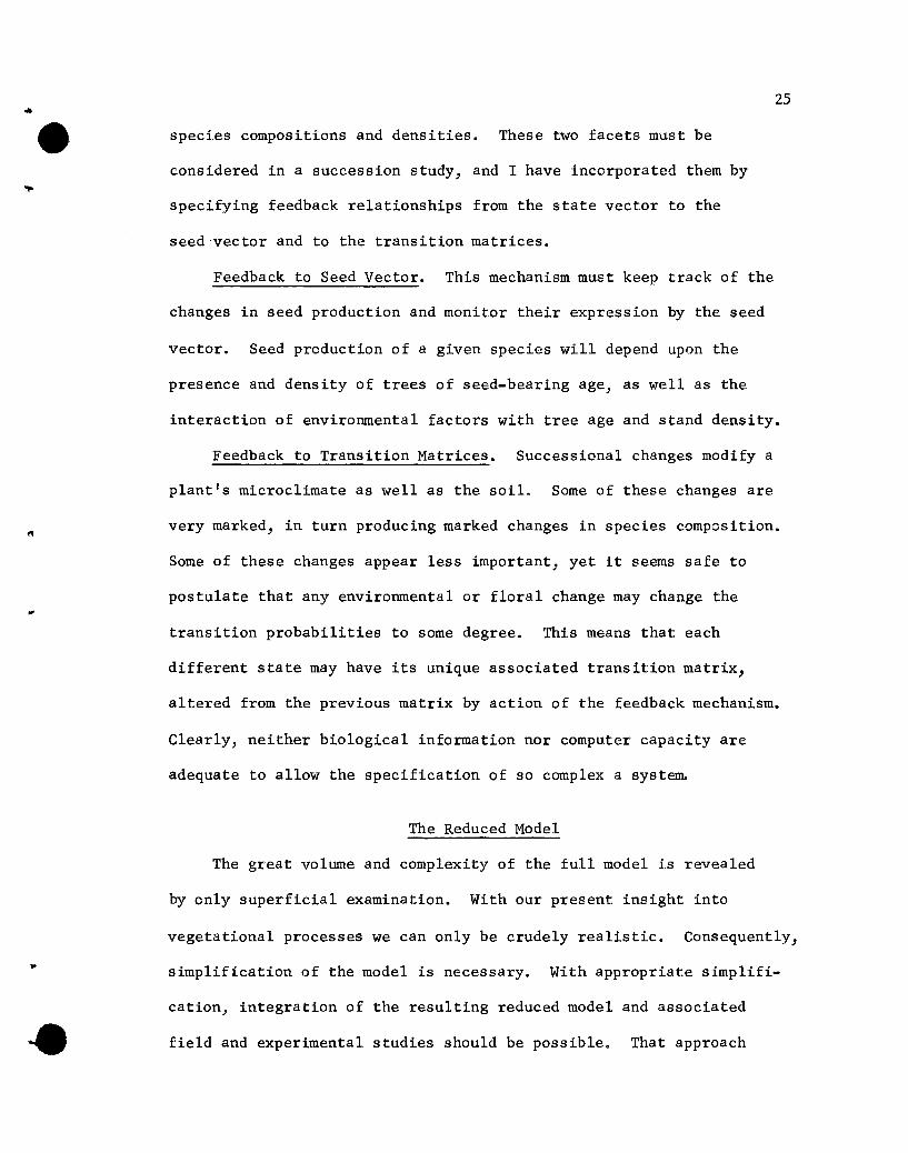
Illustration of Reduced Model

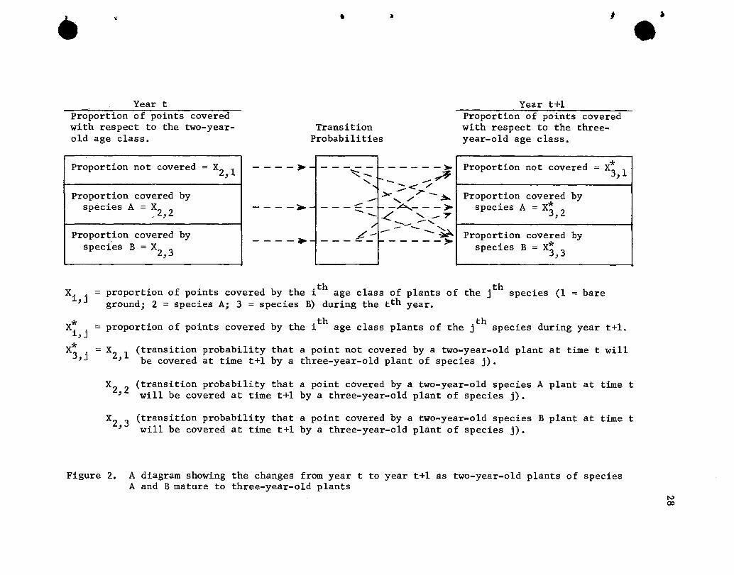
Figure 2 shows the changes from time t to time t+l for one age

group, the 2-year-01d plants in a vegetation comprised of two species,

A and B. Similar illustrations apply to all other age groups speci-

fied in the reduced model.

The State Vectors

The use of age group-specific states is justifiable at our

present stage of understanding successional processes. Two of the

most important facets of vegetation development are selection and

competition, yet they are poorly elucidated for most vegetation

types. Some investigators (see Literature Review) indicate that

competition occurs only if plants are more or less equal; an over-

story tree and understory seedling relationship is not a competitive

• i, It I I•

Year t Year t+1Proportion of points coveredwith respect to the two-year­old age class.

TransitionProbabilities

Proportion of points coveredwith respect to the three­year-old age class.

Proportion not covered = X2 1,Proportion covered by

species A = X2 2, ,

Proportion covered byspecies B = X2 3,

----~-

----~-

- - - -.-

----- -----~~ ;Ie::::- _ _r'

-< />r- .7'"_

...... ./ ~--- -,6....---~-< ...... _""7'

...........-- --,-- - .......? __ - - -:;...4.

----- -----~

Proportion not covered = x;, 1

Proportion covered byspecies A = x; 2,

Proportion covered byspecies B = x; 3,

X2

1 (transition probability that a point not covered by a two-year-01d plant at time twill, be covered at time t+1 by a three-year-01d plant of species j).

= proportion of points covered by the i th age class of plants of the jth species (1 = bareground; 2 = species A; 3 = species B) during the tth year.

= proportion of points covered by the i th age class plants of the jth species during year t+1.*X. J.~,

X* . =3,J

x. J.~,

X2 2 (transition probability that a point covered by a two-year-01d species A plant at time t, will be covered at time t+1 by a three-year-01d plant of species j).

X2 3 (transition probability that a point covered by a two-year-01d species B plant at time t, will be covered at time t+1 by a three-year-01d plant of species j).

Figure 2. A diagram showing the changes from year t to year t+1 as two-year-01d plants of speciesA and B mature to three-year-01d plants

N00

~

•

•

29

one, those investigators claim, but solely one in which the overs tory

tree exerts its influence through modification of important facets

of the environment such as light regimes, soil moisture, etc. With

trees, the more or less equal plants are those of the same age; hence

specifying states on an age class basis insures that we retain in

the model those states influenced strongly by competitive relation­

ships. The overs tory tree-seedling state would not be retained, but

the overstory tree influences would be incorporated in the functional

relationships specified for the appropriate seedling transition

matrices.

The age group approach allows detail in specifying states within

age groups, without increasing the number exhorbitantly. For example,

n important states might exist and need elucidation for seedlings and

m for a specific age of overstory trees. If the age group approach

was not used, n x m states would need to be specified to give us the

necessary detail for both the seedlings as well as the overs tory

trees. The simplification using age groups is substantial, especially

if many combinations of overs tory trees produce essentially identical

environmental changes.

Another reduction in number of states involves specifying age

groups of unequal length. The probabilities for continuance of a

state or for going from one state to another for a particular species

undoubtedly change greatly during the first few years of a plant's

growth. For example, the probability that a seedling survives to

a one-year~old plant is probably much different than the survival

probability to two years of a one-year-old plant. As the plant

~

•..

•

30

grows older, however, the year~to-year transition probabilities

probably change very little until advanced age is attained. For

many years of a plant's life those probabilities are probably near 0

or 1 for a change of species or a continuance of one, respectively.

If the probabilities are relatively unchanging for a number of years

in a plant's life and if the probability for changing states is very

small, combining of a number of ages into new age groups may be

warranted. The advantages, of course, would be fewer parameters to

estimate and a decrease in computational effort. Changes in transi­

tion probabilities and states undoubtedly contain information regard­

ing vegetation processes. If we combine a number of ages possessing

such changes, such information for the new age groups would be un­

available. Therefore, the new age groups should have state changes

involving only one step, i.e. from state i to state j and not through

an intermediate state k. Requiring that the ages being combined

have small probabilities of state changes insures that the above

condition is met.

The seedling stages are very critical stages of a tree's life,

often with rather high mortality rates applying. Each of the first

two or three years should be an age group, or perhaps even more than

one if the situation warrants. As the tree grows older, however,

the evidence in favor of combining ages increases and various ages

should be combined.

Seed Vector

I have incorporated two simplifications into the reduced model

that affect the seed vector. The first simplification is the single

••

•

31

vector specification for seeds states. That simplification is

predicated on the assumption that all seeds justifiably can be lumped

in one age group. The second simplification, which influences the

seed state values as well as the feedback relationships, involves

specifying a vector called MAX SEED. That vector contains the

largest permissible seed cover values for each species, reflecting

field investigation findings that seed production in certain species

may level off, or even decrease, as the stand densities increase

beyond certain limits. In the present model, I did not incorporate

feedback relationships that would decrease seed production for

densities exceeding certain values, but only specified the maximum

seed values.

Transition Matrices

Defining states only within age groups requires a redefinition

of the transition matrix. If the state vectors are restructured to

reflect the within age group competitive relationships, the transi­

tion probabilities also must be restructured to reflect the fortunes

of plants in those age groups. That is, the probabilities of

individuals of an age group dying or surviving to the next age group

are the ones of primary concern. The other transitions, such as

transition from coverage by a m-year-old individual to coverage by a

m+lO-year-old individua~ probably result primarily from changed

environmental conditions imposed by the older age group and not by

interplant relationships. Hence, transition probabilities, which

are functions of environmental factors, for transition from one age

group to the next contain much of the relevant information. The many

•

•

32

possible transitions from one age group to a much different age

group probably individually contain very little additional information

and a justifiable simplification is to delete them in the specifica=

tion of transition matrices. Consequently) in the reduced model

matrices of order equal to the number of species in the succession

plus one and whose entries are transition probabilities are specified

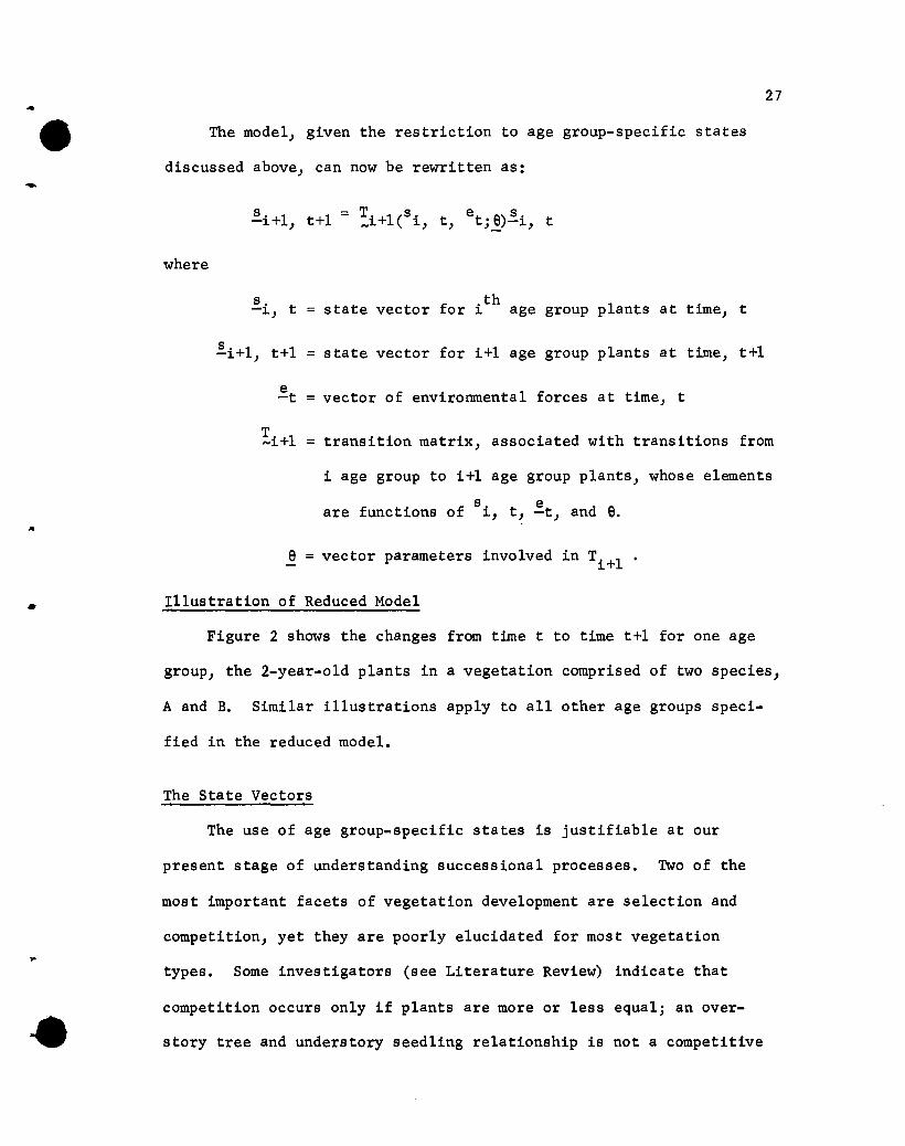
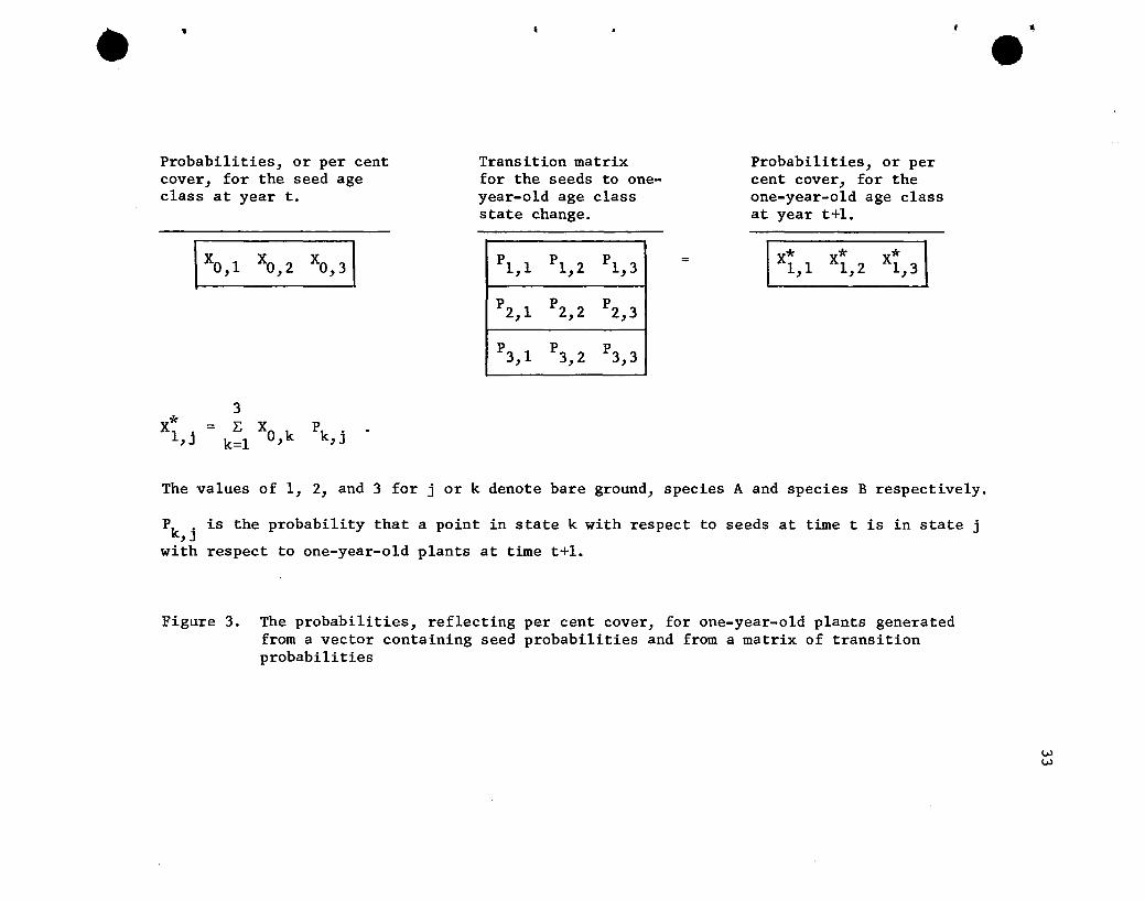
for every age group except seeds. The first transition matrix

transforms the seed vector into probabilities reflecting the per cent

cover for one-year-old) or first age group plants (Figure 3). These

first age group values are then transformed by the second transition

matrix, and cover values for age group two plants result. This

process continues for older age groups and their associated transition

matrices.

Feedback in Reduced Model

At our present stage of knowledge trying to specify in detail

the functional relationships of plants probably is an exercise in

futility. Only crudely realistic characterizations of the relation-

ships are possible with our present knowledge. Some general simplify-

ing assumptions are possible, however; a reasonable one is that the

elements of ~ not influenced by plants are time-invariant and can be

absorbed in 9. Some of the elements in e that are influenced by

plants, such as light intensity and radiation at the ground surface)

can be related to elements in ~t associated with the overs tory

vegetation. Such elements in e can thus be related to elements of T

in terms of elements in s. For the remaining elements in _e and-t

for s , the initial specification of their relationships to the-t

Probabilities, or percent cover, for theone-year-01d age classat year t+l.

•Probabilities, or per centcover, for the seed ageclass at year t.

IXO,l Xa,2 Xo,31

Transition matrixfor the seeds to one­year-old age classstate change.

P1 1 P1 2 P1 3, , ,

P2 1 P2 2 P2 3, , ,

P3 1 P3 2 P3 3, , ,

= *X1,1 *X1,2 *Xl 3,

~•

* ­Xl . -,J

3l: X

k=l O,kPk .

,J

The values of 1, 2, and 3 for j or k denote bare ground, species A and species B respectively.

Pk . is the probability that a point in state k with respect to seeds at time t is in state j,J

with respect to one-year-01d plants at time t+1.

Figure 3. The probabilities, reflecting per cent cover, for one-year-01d plants generatedfrom a vector containing seed probabilities and from a matrix of transitionprobabilities

VolVol

•

•

34

elements of the T's should be simple and straightforward. As more

insight and knowledge is gained, additional complexity reflecting

greater realism can be incorporated.

Feedback to Seed Vector. I based the seed feedback relationship

on the assumption that the change in seeding rate caused by a change in

the area covered by the i th age group plants of species j is propor-

tional to that change in cover. The exact change in seed probabili~

thties caused by i age trees is the product of the change in cover

thof the i age trees and the relative measure of the influence of

that age group.

The relative measure of an ag~ group's influence is contained

in a matrix called a RESEED matrix, that has as col~n vectors relating

to each species in the succession. The matrix has a row per age

group other than seeds, and a column for each species and for bare

d h i h .th d th 1groun. T e entry n t e 1 rowan j co umn is a relative

measure of the influence of the ith age-group trees of species j on

the seed probabilities for that species.

A facet of the reduced model that influences the exact specifica-

tion of feedback relationships is the age group feature. Suppose the

thi age group consists of a ten-year interval, say for trees 50 to

60 years old. At the conclusion of a ten~year period, the changes

in area covered by a certain species' trees of that age reflect

changes that are occurring during the interval, and that influence

seed probabilities as they occur. However, the change is calculated

only at the conclusion of the interval, and any feedback relation-

ships must await that calculation. As a result, if that age group

•

•

35

has a large influence on seed probabilities, substantial changes in

seed probabilities will occur every ten years, but in the interim

they will be relatively unchanging. This is certainly an unnatural

feature in a succession simulation, and would produce a spasmodic

progression of the simulated succession. To counteract this feature,

I have, in my simulation runs, arbitrarily apportioned the change

into as many equal parts as there are years in the interval, thus

producing gradual changes in seed probabilities and in progression

of succession. This procedure causes a slight lag in interaction

effects, however, and hence slows the speed of successiono

The feedback equation used in the model is as follows. Let,

X,. the change in per cent cover of age group i plants of1J

species j.

T" relative measure of the influence of ith

age trees of1J

species j on that species seed probabilities. These

values are in the RESEED matrix.

h, number of age-classes (years) combined to form age1

group i.

Sj seed probability for species j.

AS, = change in seed probability for species j.J

m number of age groups other than seeds.

Then

m= L: (/SA, •• T, , /h,)

i=l 1J 1J 1

Let Sj be the adjusted seed probability. Then,

S"':J

"•

•

36

Feedback to Transition Matrices. The P.. IS, specified on an~,J

age-specific basis, are functions of t~e, environment and the

species composition of the stand. That is, for the t age group,

As I have discussed earlier, specifying the functional relationships

for the P. j'S is very difficult at our present stage of knowledge.~,

Perhaps our first concern should be to determine which environmental

factors and species characteristics causally influence vegetation

and when during a plant's life and the course of succession they are

important. The reduced model is structured to contribute to those

objectives.

I have incorporated the transition feedback relationships into

the reduced model by specifying certain equations to adjust the

transition probabilities. I specified that the change in the

probability that a species maintains itself at a point from age i to

i+1 is proportional to the product of the change in per cent cover

of the species interacting with it and its own per cent cover. That

is, the change in the transition probability that a point covered by

species j in age group i continues to be covered by j in age group

i+1 is proportional to the product of the change in per cent cover

of interacting species k, say in age group t, and the per cent cover

of species j. The per cent cover of the interacting species is included

because when it is scarce its effects on the species interacted with

will be smaller than when it is abundant. The equations for the

transition probability changes follow. Let,

•37

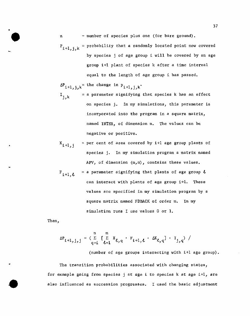
n = number of species plus one (for bare ground).

p. 1 . k probability that a randomly located point now covered1+ ,J,

by species j of age group i will be covered by an age

group i+1 plant of species k after a time interval

equal to the length of age group i has passed.

~P'+l . k1 ,J,I. kJ,

Then,

the change in p. 1 . k'1+ ,J,a parameter signifying that species k has an effect

on species j. In my simulations, this parameter is

incorporated into the program in a square matrix,

named INTER, of dimension n. The values can be

negative or positive.

per cent of area covered by i+1 age group plants of

species j. In my simulation program a matrix named

APV, of dimension (m,n), contains these values.

a parameter signifying that plants of age group t

can interact with plants of age group i+1. These

values are specified in my simulation program by a

square matrix named FDBACK of order m. In my

simulation runs I use values 0 or 1.

n m(~ [~X, . F'+l ' . 6X, J. I. ) /q=i t=l ~,q 1,~ ~,q J,q

(number of age groups interacting with i+1 age group).

•The transition probabilities associated with changing states,

for example going from species j at age i to species k at age i+1, are

also influenced as succession progresses. I used the basic adjustment

••38

specified above, multiplying its value by the transition probability

being adjusted. Hence, the changes in these transition probabilities

are proportional to the probabilities themselves. The equation for

this change is

M'i+l,j,k

m( ( L: X-e, k

-e,=1 '

•

(number of age groups interacting with i+1 age group))

The corrected probabilities are, letting P* be the corrected values,

p* = p + t.Pi+l,k,j i+l,k,j i+l,j,k

In this reduced model I have included only one matrix INTER for

species interactions and only one, FDBACK, for feedback effects. If

I had included a separate interaction matrix for each species, I

undoubtedly could have obtained greater realism. However, considering

the lack of suitable succession data, and hence the basis for

estimating the elements of those matrices, as well as the increased

costs of simulation that a more complex model would produce, I

concluded that the initial modeling should not strive for excessive

detail. Actually, when suitable data and insight are available, it

may be necessary to specify for each age group a matrix of size

(n, n, n-1, m) before the interrelationships between species and age

groups can be evaluated and simulated .

•

•

•

39

RESULTS

The reduced model was converted to a computer program using

FORTRAN IV language (Appendix A). An IBM 360 Model 40 computer was

used to produce five simulated successions involving only two plant

species. Those successions, based on data sets listed in Appendix B,

are contained in Appendix C.

Data Sets

I attempted to locate data sets that would be suitable for

illustrating my modeling approach. A thorough search of the litera­

ture failed to reveal any set that would be useful. The essential

criteria missing from all sets were adequate information regarding

the age and fortunes of individual plants during some time interval,

and the spatial relationships of those plants and their neighbors.

Consequently, I had to fabricate data sets.

State Vectors

The initial state vectors have zeros for both plant species

and 1.0 values for bare ground entries. Such values result from

the specification that the simulated successions are based on re­

invasion of a denuded area.

Seed Vector

I could not find any data directly specifying the values for

entries in the seed vector, but numerous papers reporting seed

production for commercially important lumber species exist (see

Literature Review). The data reveal substantial temporal and spatial

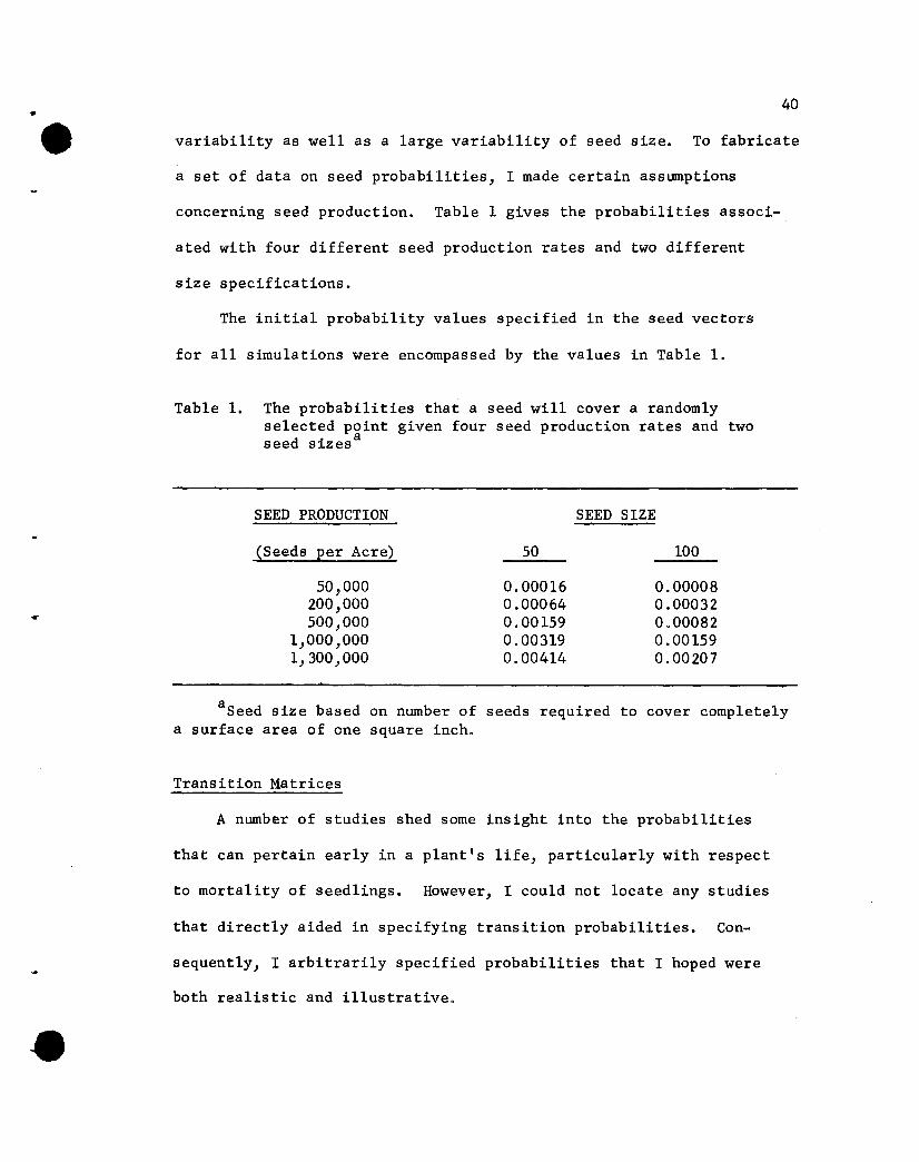
•40

variability as well as a large variability of seed size. To fabricate

a set of data on seed probabilities, I made certain assumptions

concerning seed production. Table 1 gives the probabilities associ-

ated with four different seed production rates and two different

size specifications.

The initial probability values specified in the seed vectors

for all simulations were encompassed by the values in Table 1.

Table 1. The probabilities that a seed will cover a randomlyselected point given four seed production rates and twoseed sizesa .

SEED PRODUCTION

(Seeds per Acre)

50,000200,000500,000

1,000,0001,300,000

50

0.000160.000640.001590.003190.00414

SEED SIZE

100

0.000080.000320.000820.001590.00207

•

a Seed size based on number of seeds required to cover completelya surface area of one square inch.

Transition Matrices

A number of studies shed some insight into the probabilities

that can pertain early in a plant's life, particularly with respect

to mortality of seedlings. However, I could not locate any studies

that directly aided in specifying transition probabilities. Con-

sequently, I arbitrarily specified probabilities that I hoped were

both realistic and illustrative .

•

•

Feedback Relationships

The general feedback relationships used in the reduced model

are discussed in the section The Reduced Model.

Feedback Relationship to Seed Vector. Although a number of

studies have dealt with the influences of stand age and densities

on seed production, none have specified the relationships existing

between the stand characteristics and seed production; only observa­

tions were reported. The lack of detail in describing the stand

characteristics prohibited using the data as bases for estimating

the re1~tive influence of each age group on seed probabilities.

Hence, I arbitrarily specified values for the RESEED matrix.

Feedback Relationship to Transition Matrices. No data sets

exist as bases for estimating the FDBACK matrix values used in the

feedback relationship. Consequently I used a simple assumption as a

guide for setting those values. I assumed that older age classes

influenced the fortune of younger age classes, but that the reverse

situation was sufficiently inconsequential to warrant its exclusion.

I also assumed that all existing relationships were inhibitory.

The values used in the INTER matrix differ from simulation to

simulation. The specific values chosen were designed to illustrate

interspecific influences, and were not based on any existing data

sets.

The Data Used

The five data sets used are identical except for the INTER and

RESEED matrices. The differences are illustrated in Table 2. In

Data Set 1 the -1 value in the second and third rows of the second

41

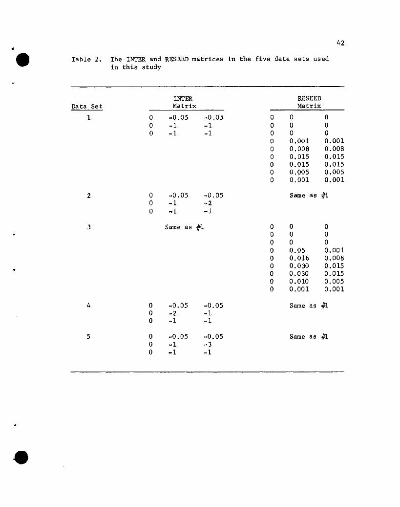
• Table 2. The INTER and RESEED matrices in the five data sets usedin this study

42

INTER RESEEDData Set Matrix Matrix

1 a -0.05 -0.05 a a aa -1 -1 a a aa -1 -1 a a a

0 0.001 0.0010 0.008 0.0080 0.015 0.015a 0.015 0.0150 0.005 0.0050 0.001 0.001

2 0 -0.05 -0.05 Same as #1a -1 -20 -1 -1

3 Same as #1 0 0 0a a 00 0 00 0.05 0.0010 0.016 0.008

• 0 0.030 0.0150 0.030 0.0150 0.010 0.005a 0.001 0.001

4 a -0.05 -0.05 Same as #1a -2 -1a -1 -1

5 a -0.05 -0.05 Same as #1a -1 -3a -1 -1

•

•

•

43

and third columns specify that species A and B have equal se1f- and

alien-inhibiting effects; in Data Set 2 the -2 value in the third

column of the second row specifies that species B has twice the

alien-inhibiting effect on A that A does on B, as well as twice the

effect of any self-inhibiting influence. The RESEED matrix in Data

Set 1 reveals equal effects for the two species of various age seed-

bearing trees on seeding rates; in Data Set 3 the values in the

species A column are approximately twice those in the species B

column, reflecting an influence on seeding rates by seed-bearing

trees of species A that is twice that by similar age trees of species

B. Data Sets 4 and 5 differ from Set 1 only in the INTER matrix~.

values. In Data Set 4 the self-inhibiting effect of A is twice that

of any other inhibiting effect and in Set 5 the alien-inhibiting

effect of B on A is three times that of any other inhibiting effect.

Results of the Simulations

The results of the five simulations are listed in Appendix C.

Before considering the individual simulations some general comments

concerning cover values are necessary. The cover values for the

different age groups in year 10 of Simulation 1 (see Appendix C)

will help illustrate aspects that need to be kept in mind.

The one-year-01d seedlings show cover values of .076 for both

species. The .076 values repres~nt the portion of the ground

covered by those plants, assuming that no overlapping of species A

and B one-year~old plants exists. If one-year-old plants of the

two species overlapped, but a supplementary specification was used

rather than a two-species state designation, the .076 value would

•

•

44

represent the proportion of the area covered, with respect to one­

year-old plants, solely by species A (or B) plants plus part of

the area covered jointly by A and B plants. The .848 value represents

the proportion of the area not covered by one-year-01d plants.

The cover values for the different-age plants of a species are

not additive. That is, the .076, .182, .212 and .109 values for

the 1-, 2-, 3- to 4-, and 5- to 8-year-01d plants of species A do

not give a sum that denotes the total proportion of the area covered

by species A, for overlapping of different-age trees of A could

occur. The sum would equal the proportion of the area covered by A

only if no overlapping of different-age species A plants occurred,

a highly unlikely situation. Hence, the traditional measure of a

species' cover, the percentage of the ground covered by plants of

that species, cannot be obtained from the simulated results. Only

if the states were all possible combinations of plants of any species

and ages would a sum be appropriate for giving the traditional

measures of cover. That aspect should be kept in mind when evaluating

the results of the simulations.

If the assumption that the different-age trees are randomly

distributed can validly be made, the traditional cover values

can be estimated. An estimate of bare ground would be the product

of the bare ground values for every age class. An estimate of the

cover for any specific species would be the sum, for all combinations

of one cover category per age class in which at least one age class

has the cover entry pertaining to the species in question, of the

products of each combination's cover values. If randomness cannot be

~

•

•

45

assumed, the distribution of the cover for different-age trees would

need to be known before the tradntional cover values could be

estlinated.

Simulation 1

The seed probabilities for species A and B appear to be un­

changed from their initial values of .0010 at the tenth year of

succession (see year 10, simulation 1, Appendix C). However, if

additional significant digits were included, the values for each

species would have shown a change from the .00100 initial value to a

.00101 value at year 10. The change is very small, due to the fact

that only plants of the 5- to 8-year-old group, of those present at

year 10, are influencing seed production. That aspect is revealed

by the zero values in the second and third columns of the 1-, 2-,

and 3- to 4-year-01d age group lines in the RESEED matrix, and the

.001 values in those columns for the 5- to 8-year-01d age group line.

The adjustment equation is listed in the section Feedback to Seed

Vector.

Plants from older age groups gradually appear in the stand as

succession progresses and stand density increases. By year 80 the

cover values for the younger age classes are changing only slightly,

and the seed cover values have increased from the initial value of

0.0010 to 0.0023.

The increase in cover continues for all age classes throughout

succession, but the rate of increase slows as succession progresses.

During the 50-year span from year 100 to year 150, only age groups

57-80 years and greater than 80 years show any appreciable change.

•

•

46

By year 150 the succession is relatively unchanging with respect to

cover, and by year 177 the stand has met the requirement I specified

for an unchanging forest: none of the transition probabilities

change by more than .005 during two consecutive adjustments of each

transition matrix.

The seed vector at the termination of succession had probabilities

of coverage of .0030 for both species. The identical values reflect

the fact that equal specifications for both species were made in all

facets of the data set. The equality for both species persists in

all aspects of the simulated succession.

The coverage values at termination increase with age for the

first through the sixth age groups; the values then decrease for the

last three age classes. Although the seed probabilities for the

two species increased by a factor of 3 from year 10 to year 177,

the coverage values for the first 3 age groups increased only by

approximately 10 per cent during that interval. The difference

reflects the adjustments made to the transition probabilities as

succession progressed.

The adjustments made to the transition probabilities are

influenced by the values in the FDBACK and INTER matrices (see

Feedback to Transition Matrices). For example, the first row of

the FDBACK matrix in Data Set 1 has as values two zeros followed by

seven ones. Those values indicate that plants of age groups 1 and 2

years cannot influence the transition probabilities in the first

transition matrix but that the plants of the 7 older age classes

potentially can. The last row of the FDBACK matrix has all zeros,

•

•

•

47

indicating that none of the age groups can modify the transition

probabilities connecting the last two age classes.

Even though a value of one appears in the FDBACK matrix, indicat­

ing that plants of a certain age class have the potential of modifying

the transition probabilities in a specific transition matrix, the

question as to which probabilities are modified when the cover

values for a given species change is not answered. That answer is

given by the INTER matrix. For example, the FDBACK matrix in Data

Set 1 has a 1 in the third column of the first row, indicating that

the 3- to 4-year-01d plants potentially can modify the probabilities

in the first transition matrix. The -1 value in the third column of

the second row of the INTER matrix indicates that species B has an

adverse effect on species A. That is, as the population of species

B increases, its inhibiting influence on A increases. When that

value is combined with the FDBACK matrix, as it is in the adjustment

equation (see page 43), the resulting combination determines which

age group plants of a species interact with specific age group

plants of other species. As I indicated above, both species are

equally se1f- and alien-inhibiting in Data Set 1; the four -1 values

in the INTER matrix denote that fact. The -.05 values in columns 2

and 3 of row 1 indicate that as the population of species A and B

increases, the probability that a point continues to be covered by

bare ground decreases.

The specifications used for the FDBACK and INTER matrices in

Data Set 1 caused adjustments that produced the final transition

matrices listed in Appendix C. Only the final ones have been included

•

•

•

48

in the simulation resultsj the initial ones, of course., are listed

in the data set.

The transition probabilities undergoing greatest modification

were those associated with changes from one species to another in

the younger age classes. For example, the probability that a point

covered by a one-year-old plant of species A is covered one year

later by a two-year-old plant of species B changed from .040 at

the start of succession to .068 at year 177. The probability change

associated with the one-year-old species A plant-bare ground state

change only varied from .010 to .002 during the same period. The

larger differences associated with species-to-species changes reflect

the fact that the absolute values of the INTER matrix entries

associated with species-to-species effects are greater than those

for species-to-bare-ground effects (!.~., 1 versus .05).

The Other Simulations

Data Set 2 differed from Set 1 only by the fact that the alien­

inhibiting effect of species B on A was twice the value in Set 2

that it was in Set 1 (-2 versus -1). The depressing effect of B

on A is very evident in the final year of the simulation, year 369.

At that time, in most age classes the cover values for species B were

three times greater than those for A. In addition, the seed prob­

abilities for A were only 0.0019, whereas those for B had reached the

maximum allowable level, 0.0040.

The influence of B also is very evident in the transition

matrices values. For example, in transition matrix 2 the probability

that a point covered by a one-year-old species A plant will be covered

•

•

•

49

a year later by a two-year-old species B plant changed from an

initial value of 0.040 to a final one of 0.234. The reverse species

change, B to A, changed from the initial 0.004 value to a final one

of nearly zero.

The different cover values for the two species result jointly

from different seeding rates and different transition probabilities.

In an attempt to ascertain which of these were most influential,

another simulation was run that was based on a data set, Data Set 3,

in which the competitive relationships were the same for both

species; but the influence of the seed-bearing-age trees on seeding

rates was approximately twice as great for species A as it was for B

(see Table 2). The initial seeding rates were identical for the

species.

The influence on cover values of the differentially changed

seeding rates was slight. In year 225, the cover values were

approximately the same for both species and the final transition

probabilities had changed only slightly from the initial ones. The

final seeding rates, however, were quite different, being 0.0040 and

0.0029 for A and B respectively. Apparently in my model the seeding

rates are unimportant and the influence changing cover values must

be the transition probabilities. As an aid in determining whether

self-inhibiting effects produced greater changes in transition

probabilities than did alien-inhibiting ones, two additional data

sets, Sets 4 and 5, were run. In Data Set 4, the self-inhibiting

effect of Species A was twice as great as any other inhibitory

effect, and in Set 5 the alien-inhibiting effect of B on A was three

times larger than any other.

••

•

50

The results from Simulations 4 and 5, in conjunction with

Simulation 2, clearly show that the alien-inhibiting effect produces

much greater changes in transition probabilities, and consequently

cover values, than does the self-inhibiting effect. That result,

of course, is an obvious consequence of the feedback equations.

The adjustment to the transition probabilities pertaining to state

changes is proportional to the cover values. Hence, the self­

inhibiting effect that would cause that species to be replaced by

another produces less change on the associated transition prob­

abilities as the species cover value decreases. The change

produced by the alien-inhibiting effect does not decrease as the

inhibited species cover value decreases •

...

•

..

•

51

DISCUSSION

Aims and Accomplishments of This Modeling Study

The relationships within and between the floral elements and

the environmental factors must be explained in a causal context if

we are to understand the processes involved in shaping vegetation.

Field observations of natural vegetation are essential for identify­

ing the existence of the relationships. For explaining the relation­

ships in a causal context, however, field observations by themselves

are inadequate. Theoretical and experimental studies must be

integrated with a field study. I am not implying that all three

must be conducted simultaneously. I am implying that the results

from any of the three must be meaningful and interpretable in terms

of the others, however. If that condition is satisfied, one

theoretical approach, modeling, can be a powerful analytic tool in

vegetation studies. That consideration substantially influenced the

structure of my succession model, for gaining insight into

successional processes is the primary objective of this modeling

effort.

I believe that this modeling study successfully accomplishes

its primary objective, for this model can be integrated with a

properly structured field study to provide insight into successional

processes. An example of what can be done will illustrate that point.

Suppose that we wish to evaluate the influence on survival of 1-,

2- and 3-year-old plants of species A caused by neighboring species B

plants. The neighboring plants, if they do not cover the sample

point, are not specified in the state for that point; the presence

~

•

•

52

of those plants is reflected in the model only through plant-modified

environmental factors. However, strong competitive relationships

might exist that influence survival of the young species A plants,

with very little evidence of those relationships manifested by the

plant-modified environmental factors. Only by evaluating survival

with respect to the neighboring plants can those competitive rela­

tionships be revealed. That evaluation is possible by judiciously

partitioning the sample space on the basis of the neighboring plant

composition. Simulations can then be run for those subsets of sample

points of interest. The differences exhibited by the different

simulations will furnish insight into the competitive relationships,

as well as aiding in delimiting which experimental studies are

needed to further elucidate the consequential inter-specific relation­

ships.

Many other partitionings of the sample space also are possible;

the above approach can be used with them as well. The limitation

to using this approach is not determined by the model, but is

determined solely by the data collected in the field study.

Characteristics of an Associated Field Study

Even a cursory examination of vegetation reveals that

vegetation is not, either temporally or spatially, a random assortment

of species. Additional examination also reveals that the vegetation

possesses variability, both spatially and temporally. These two

aspects, nonrandomness and variability, are of concern to plant

ecologists for these two are manifestations of the relationships

existing within and between the floral elements and the environmental

•

•

53

factors and of the temporal and spatial variability of the environ­

ment. Measurement of characteristics that provide information

concerning the relationships, and the ability to relate the informa­

tion to the nonrandomness and variability of vegetation and the

variability of the environment) are essential attributes of a field

study.

Kinds of Data Needed

The fortunes of propagules and individual plants determined

the vegetation of an area. That is) the pattern of dispersal of

propagules, and the response of propagules and individual plants

to their environment, which includes the adjacent vegetation, deter­

mine which plants will occupy a given space at a given time.

Consequently, vegetation change is a result of modification or

replacement of individual plants. Knowing how, why and when they

change and knowing the environment of an area, including the vegeta­

tion-modified component of the environment, are essential in order

to understand vegetation processes. Repeated measurement of

individual plants and their environments is the kind of data that

leads to such understanding.

Selection of Study Areas

Two considerations largely govern the selection of study areas.

The first concerns the type or kind of succession, !.~. a pine-oak

succession in the southeastern United States or an aspen--white

birch--white spruce succession in northern North America, and the

second, the geographic locations •

~

••

•

54

Selecting the Type of Succession. Most ecologists agree that

the degree of complexity in ecological systems increases with increas­

ing diversity of species in the system. If that concept holds, and

considering the number of transition and seed probabilities and

feedback relationships that must be specified in this succession

study, the number of species comprising the succession is a criterion

meriting attention when selecting succession type. A succession

involving only four or five tree species seems the most desirable

for basing the initial field studies. Even then, the number of

parameters to be estimated will be large, but succession involving

fewer species, and hence fewer parameters, will lack the mu1ti­

species interactions, which probably are very important facets

of more complex situations. A reasonable compromise between complex­

ity and realism seems to be a succession involving four or five

species of trees.

A successional type having a rapid successional rate and a

relatively short time to completion is desired. Age groups of only

a few years each will be possible and relatively few age groups will

be needed.

Selecting the Geographic Locations. Since even a rapidly

proceeding succession m&y require more than 100 years for completion,

studying only one plot through the entire process is not feasible.

Rather, a number of different stands reflecting different levels of

successional maturity must be studied concurrently.

Selection of the specific stands or study plots depends on the

availability of the required age groups and the perceptible or

-••

•

55

suspected historical differences and current environmental differences.

The plots should be proximally located to reduce spatially-related

environmental differences, but selection should also serve to reduce

other physiographic and topographic differences as much as is feasi­

ble.

Study plots must be selected so that plot to plot differences do

not substantially modify or change the succession pattern or the

parameter values. In fact, evaluation of the successional data

requires an assumption of no consequential plot to plot effects.

Any stand to stand differences in parameter values or feedback

relationships then can be assumed to be due to different levels of

maturity and not to other factors. With proper replication this

assumption can, and should, be tested, but extensive replication for

a succession of long duration would require a large number of study

plots. Again, a relatively short-term succession is an advantage.

Characteristics to Use in Determining State

A number of characteristics could be used in determining the

state at a point. The selection of characteristics primarily depends

on their relevance to the successional process and the ease with

which they can be measured.

Relevance to the Successional Process. The characteristics used

should be an important feature in the successional process and

should reflect substantive changes in succession. For example, a

characteristic could be the covering of a point by the stem of a

tree; for a specific age group a point could be covered by the stem

of a tree from any of the species or be uncovered. Once a point is

••

..

•

56

covered by a stem in any age group, the states in all other age

groups could only be the uncovered state. Substantial changes could

be occurring in the stand, for example the specific tree covering

the point as well as other individuals of the same species in the

stand could be degenerating steadily, yet states based on the stem

characteristic largely would remain unchanged. In essence the

characteristics used in state determination must be meaningful ones

reflecting stand changes.

Ease in Measuring. Ease and economy i.n measuring a characteris­

tic are very desirable features, especially in light of the large

number of sample points needed in a succession study. Preferably,

only a visual inspection should be needed to determine state. The

cover by aerial parts characteristics satisfies this reqUirement.

However, the selection of characteristics for a specific study must

depend on the evaluation of attributes with respect to that particular

study.

General Characteristics of This Model

A few general characteristics of this model warrant discussion.

They concern the point orientation of the model, the simplifications

used and relating the reduced model to the "whole" system.

Point As a Sample Unit

The model is developed with respect to points on the land

surface, yet I have stressed above (see section Kinds of Data Needed)

that the fortunes of individual plants is the kind of information

needed in order to understand successional processes. Although points

~

••

•

57

are the sample units, the information obtained concerns plant

fortunes, for the repeated measurements at a point can be assumed

to be repeated measurements of the same individual plants. That

assumption is possible because I used cover on an age-class and

species-specific basis. For example, if our field data showed that

a point was covered at year t by a lO-year-old species A plant and

a l-year-old species B plant, at year t+l by an ll-year-old species A

plant and a 2-year-old species B plant, and at year t+2 by a l2-year­

old species A plant but not by a species B plant, the conclusion

that only two individual plants were measured during that three-year

span and that the younger plant died in its second year of life

probably would be correct. That is, the fortunes of two individual

plants were recorded.

Simplifications in the Model

Any vegetation model that approaches a one-to-one correspondence

of the vegetation and model parameters would be unmanageable. The

large number of vegetation parameters results from the large number

of species involved and the necessity of considering tUne and the

environment. In some judicious manner a decision has to be made

as to which parameters should be ignored or combined, and which

should be considered separately. In essence, what sUnplifications

should be employed in fashioning a reduced model of manageable

proportions?

Guiding Concept. The guiding concept I used in determining

model simplifications was that any detail lost by simplifying the

full model should be recoverable by using the simplified model in

•••

•

58

conjunction with associated field or experimental studies. The

state vector simplification illustrates that aspect •

Rather than defining all possible combinations for cover at a

point, only combinations within an age-group of plants were con­

sidered. Hence a point that was covered by a 3-year-old species A

plant and a 3-year-old species B plant would have a species A state

for the 2-year-old age group, a species B state for the next older

age group, and a bare ground state for all other age groups. The

point's detailed cover state, that is cover by a 2-year-old species A

plant and cover by a 3-year-old species B plant, would not be speci­

fied. In addition, transitions only from one age group to the next

older age group were considered. Consequently, transition probabili­

ties that probably contain a great amount of information regarding

inter-specific and inter-age group interactions, such as the prob­

ability that a point covered at time t by a seedling of species A

and an 80-year-old plant of species B will be covered only by an

8l.year-old plant of species B one year later, are not included in

the model. Hence the model, by itself, provides little insight into

the 80-year-old plant-seedling interaction. However, if i.n an

associated field study a collection of points has been selected using

some random selection scheme, that collection of points can be

partitioned so that one subset of points possesses the 80-year-old

plant-seedling state and the other the seedling state. Separate

simulated successions then can be run for each subset of points and

the differences assessed. Those differences should provide insi.ght

into the 80-year-old plant-seedling interaction•

••

•

•

59

In effect, the above procedure allows an investigator to

regain through partitioning of the sample space detail that was

lost by model simplification.

Simplifications Used. The two important simplifications used

to fashion the reduced model, that is specifying states solely on an

age group basis and specifying transition probabilities only for

state changes to the next older age group, were based on the belief

that inter-specific competitive relationships are influential in

determining vegetation change; such importance dictates that a

succession model include those relationships. Inter-specific

competition usually is most intense between ecologically similar

organisms; with trees, that situation probably exists with equal-age

trees. Consequently, those states defined within an age group

probably are the states in which competitive effects are most

influential. Such effects undoubtedly are manifested in the pattern

of plant survival to the next older age group. Therefore, states

defined on an age group basis and transition probabilities for state

changes to the next older age group are of sufficient importance to

warrant their inclusion in a model. The other states and transition

probabilities probably contain much less information on competition

than do the ones discussed above, and I deleted them from my model.

The states and transition probabilities I deleted contain

information about the relationships existing between plants of

different ages. With plants of very different ages, such as an

overstory tree and a seedling, the influences probably are uni­

directional. That is, the influence of a seedling on an overstory

...•

•

•

60

tree probably is negligible, with only the opposite one of consequence.

Most of the influence of any overs tory tree on a seedling undoubtedly

occurs through environmental modification such as shading, formation

of a duff layer, changed temperature regimes, etc. By measuring the

modified environmental factors, the influences exerted by an overs tory

tree can be incorporated into the model. Consequently, the loss of

information is not as great if the unequal-age states are deleted

rather than the equal-age states.

The Reduced Model and the "Whole" System

My reduced model does not treat a forest succession in its

entiretyj parts are deleted, with the information contained in the

deleted parts recoverable only by using the model in conjunction

with a field study. Is lack of treatment of the "whole" a serious

drawback?

A complex system such as forest succession has many different

facets that need elucidation. Not all facets require equal detail,

however. If our insight into a system is superficial, as is our

insight into successional processes, we cannot efficiently and

effectively structure a whole system model of a complex system, for

we do not know which facets are important or the levels of detail

required. The first task is to understand the parts comprising

the systemj this modeling effort is designed primarily for that level

of understanding.

As our level of understanding increases, we can use greater

detail and complexity in our models. That is, we can move toward

the full model. Whether we will ever reach the goal of a full model

••

•

61

is debateable, for perhaps we are intellectually incapable of

comprehehding and inter-relating at the necessary levels of detail,

all facets of a complex system. None-the-less, as we strive to

reach the full model, we will continue to increase our understanding

of the system. That consideration provides ample justification for

the approach I am advocating•

••

,

•

•

62

SUMMARY AND CONCLUSIONS

Vegetation is a complex, dynamic phenomenon. Any vegetation

study has to be structured to deal with the complexity and to consider

the dynamic aspect. Integration of field study, modeling and

experimentation can aid in coping with the complexity and evaluating

the dynamic aspect.

At our present level of understanding of successional processes,

we can build only crudely realistic models. Simplifications are

necessary. The simplifications used, however, should not cause

excessive loss of detail of the important facets of succession.

Detail should be sacrificed only for the less important facets. If

a field study is properly structured and integrated with the model,

the information lost through simplification can be regained by using

the model as an analytic tool in conjunction with the field study•

Studying the fortunes of individual plants is essential if

insight into the vegetation processes is desired. The spatial and

temporal relationships of individual plants, and their micro­

environments, are critical features needing elucidation. These

considerations demand repeated observations of individual plants.

Measuring or estimating population parameters, such as mean per cent

cover, clearly does not give us the necessary information concerning

individual plant phenomena.

Variation is a feature of vegetation that requires attention from

plant ecologists. We cannot continue to structure our vegetation

studies so that the information contained in variability is unavailable

to us. We need to structure our studies so that the extent of and

~•

•

63

causes of variability are ascertained. Both spatial and temporal

variability are of concern, of course.

The assessment of plant composition at and near randomly

selected points is a procedure demanding serious attention from plant

ecologists. With a proper sample design, with adequate measurement

of the environment, and with adequate grouping of age-classes, the

approach appears promising for studying forest succession. For

initial study, a forest succession that involves few species, has a

rapid rate of change, and attains maturity quickly is the most

desirable •

••

,

64

LIST OF REFERENCES

Allen, P. H., and K. B. Trousdell. 1961. Loblolly pine seed produc­tion in Virginia-North Carolina coastal plain. J. Forestry 59:187-190.

Anderson, D. J. 1965. Classification and ordination in vegetationscience: controversy over a non-existent problem. J. Ecol.53:521-526.

Anderson, D. J., R. C. Cooke, T. T. Elkington, and D. J. Read. 1966.Studies on structure in plant communities. II. The structureof some birch copse and dwarf-heath communities inSkjaldfannardalur, Northwest Iceland. J. Ecol. 54:781-793.

Austin, M. P., and P. Greig-Smith. 1968. The application of quanti­tative methods to vegetation survey. II. Some methodologicalproblems of data from rain forest. J. Ecol. 56:827-844.

Baldwin, H. I. 1940. Plant competition for soil moisture. Ecology21:400-403.

Becking, R. W. 1957. The Zurick-Montpellier school of phytosociology.Bot. Rev. 23:411-488.

Becking, R. W. 1968. Vegetational response to change in environmentand change in species tolerance with time. Vegetation 16:135-158.

Billings, W. D. 1938. The structure and development of old fieldshortleaf pine stands and certain associated physical propertiesof the soil. Ecol. Monog. 8:437-499.

Black, J. N. 1958. Competition between plants of different initialseed sizes in awards of subterranean clover (Trifoliumsubterraneum L.) with particular reference to leaf area and thelight microclimate. Aust. J. Agr. Res. 9:299-318.

Bormann, F. H. 1953. Factors determining the role of loblolly pineand sweetgum in early old-field succession in the Piedmont ofNorth Carolina. Ecol. Monog. 23:339-358.

Braun-~lanquet, J.Communities.

1932. Plant Sociology:McGraw-Hill, N. Y., N. Y.

The Study of Plant

•

•Braun-Blanquet, J., and E. Furrer. 1913. Remarques sur l'etude des

groupements des plantes. Bul. Soc. Languedocienne des geographicGeorge 36:20-41. (Excerpts in Kormondy, J. E. 1965. Readingsin Ecology. Prentice Hall, Englewood Cliffs, N. J.)

Cain, S. A. 1947. Characteristics of natural areas and factors intheir development. Ecol. Monog. 17:185-200.

*.

•

65

Clements, F. C. 1916. Plant succession, an analysis of the develop­ment of vegetation. Pub1. Carnegie Inst., Washington, D. C., 242:1-512.

Clements, F. C. 1928. Plant Succession and Indicators. H. W. We1sonCo., N. Y., N. Y.

Cottam, G., and J. T. Curtis. 1949. A method for making rapid surveysof woodlands by means of pairs of randomly selected trees.Ecology 30:101-104.

Cottam, G., and R. P. McIntosh. 1966. Vegetational continuum.Sci.ence 152: 546-547.

Cowles, H. C. 1899. The ecological relations of the vegetation onthe sand dune of Lake Michigan. Bot. Gaz. 27:95-117; 167-202;281-308; 361-391.

Curtis, J. T., and R. P. McIntosh. 1951. An upland forest continuumin the prairie-forest border region of Wisconsin. Ecology 32:476-496.

Daubenmire, R. 1966. Vegetation: identification of typal communi­ties. Science 151:291-298.

de Peralta, F. 1935. Some principles of competition as illustratedby Sudan grass, Ha1us sorghum sudanesis (Piper) Hitch.Eco1. Monog. 5:355-404.

Egler, F. E. 1968. The continuum concept of vegetation: responses.Bot. Rev. 34:259-267.

Gleason, H. A. 1917. The structure and development of the plantassociation. Bull. Torrey Bot. C1. 44:463-481.

Gleason, H. A. 1926. The individualistic concept of the plantassociation. Bull. Torrey Bot. C1. 53:7-26.

Goodall, D. W. 1963. The continuum and the individualisticassociation. Vegetation 11:297-316.

Harper, J. L. 1967. A Darwenian approach to plant ecology.J. Ecol. 55:247-270.

Harper, J. L., and I. H. McNaughton. 1962. The comparative biology ofclosely related species living in the same area. VII. Inter­ference between individuals in pure and mixed populations ofPapaver species. New Phytologist 61:175-188.

Keever, C. 1950. Causes of succession on old fields of the Piedmont,North carolina. Ecol. Monog. 20:229-250 •

Leak, W. B. 1968. Birch regeneration: a stochastic model. USDAFor. Sere Res. Note NE-85.

~.

•

66

Leith, H. 1968. The continuum concept of vegetation: responses.Bot. Rev. 34:291-302.

Major, J. 1958. Plant ecology as a branch of botany. Ecology 39:352-363.

McIntosh, R. P. 1967. The continuum concept of vegetation. Bot.Rev. 33:130-387.

McVean, D. N. 1955. Ecology of Alnus glutinosa (L.) Gaertn.II. Seed distribution and germination. J. Eco1. 43:61-71.

Monk, C. D. 1968. The continuum concept of vegetation: responses.Bot. Rev. 34:303-305.

Pessin, L. J.species.

1939. Root habits of longleaf pine and associatedEcology 20:47-57.

Phares, E., and N. F. Rodgers. 1962. Lmproving shortleaf pine seedproduction in Missouri. J. Forestry 60:322-324.

Poore, M. E. D. 1956. The use of phytosocio1ogica1 methods inecological investigations. IV. General discussion of phyto­sociological problems. J. Ecol. 44:28-50.

Poore, M. E. D. 1962. The method of successive approximation indescriptive ecology. Adv. Eco1. Res. 1:35-68.

Poore, M. E. D. 1964. Integration in the plant community. J. Ecol.52 (Supp1.):2l3-226.

Poore, M. E. D. 1967. The concept of association in tropical rainforest. J. Ecol. 55:46-47.

Ramensky, L. G. 1926.vegetationsdecke.

Die grundgesitzmassigkeiten in aufbau derBot. Zentra1b1. N.F. 7:453-455.

•

Shoulders, E. 1961. Effect of seed size on germination, growth andsurvival of slash pine. J. Forestry 59:363-365.

Slobodkin, L. B. 1965. On the present incompleteness of mathematicalecology. Am. Scient. 53:347-357.

Stephenson, G. K. 1963. Ten years of short1eaf pine seed crops inTexas. J. Forestry 61:270-272.

Warming, E. 1909. Oecology of Plants,. an Introduction to the Studyof Plant Communities. Translation by Percy Groom and IsaacBalfour. Clarendon Press, Oxford, England.

Wells, B. W. 1928. Plant communities of the coastal plain of NorthCarolina and their successional relations. Ecology 9:230-242.

~.

•

•

67

Whittaker, R. H. 1952. A study of summer foliage insect communitiesin the Great Smoky Mountains. Eco1. Monog. 22:1-44.

Whittaker, R. H. 1956. Vegetation of the Great Smoky Mountains.Eco1. Monog. 26:1-80.

Whittaker, R. H. 1962. Classification of natural communities. Bot.Rev. 28:1-239.

Whittaker, R. H. 1967. Gradient analysis of vegetation. Bio1. Rev.49:208-264.

Yarrenton, G. A. 1966. A plotless method of sampling vegetation.J. Eco1. 54:229-237.

Yarrenton, G. A. 1967a. Organisma1 and individualistic concepts andthe choice of vegetation analysis. Vegetation 15:113-116.

Yarrenton, G. A. 1967b. Principal component analysis of data fromsacico1ous bryophyte vegetation at Steps Bridge, Devon.III. Correlation of the variation in the vegetation withenvironmental variables. Can. J. Bot. 45:249-258 •

Yarrenton, G. A. 1969. Plant ecology: a unifying model. J. ofEco1. 57:245-250 .

....•

,

..

•

•

APPENDICES

68

~.

..

•

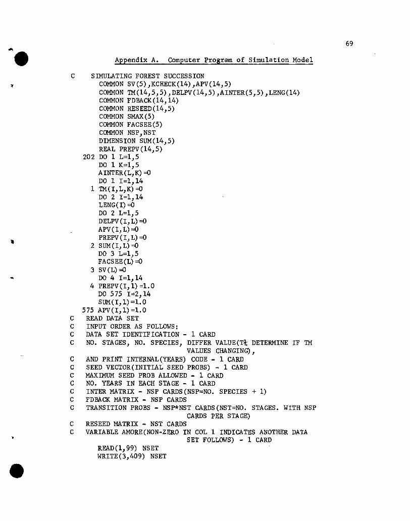
Appendix A. Computer Program of Simulation Model

C SIMULATING FOREST SUCCESSIONCOMMON SV(5),KCHECK(14),APV(14,5)COMMON TM(14,5,5),DELPV(14,5),AINTER(5,5),LENG(14)COMMON FDBACK(14,14)COMMON RESEED(14,5)COMMON SMAX(5)COMMON FACSEE(5)COMMON NSP,NSTDIMENSION SUM(14,5)REAL PREPV(14,5)

202 DO 1 L=1,5DO 1 K=1,5AINTER(L,K)=0DO 1 1=1,14

1 TM(I, L,K) =0DO 2 1=1,14LENG(I) =0DO 2 L=1,5DELPV (I, L) =0APV(I,L) =0PREPV (I, L) =0

2 SUM(I,L)=ODO 3 L=1,5FACSEE(L) =0

3 SV(L) =0DO 4 1=1,14

4 PREPV(I,l) =1.0DO 575 1=2,14SUM(I,1)=1.0

575 APV(I,1)=1.0C READ DATA SETC INPUT ORDER AS FOLLOWS:C DATA SET IDENTIFICATION - 1 CARDC NO. STAGES, NO. SPECIES, DIFFER VALUE(T~ DETERMINE IF TM

VALUES CHANGING),C AND PRINT INTERNAL(YEARS) CODE - 1 CARDC SEED VECTOR(INITIAL SEED PROBS) - 1 CARDC MAXIMUM SEED PROB ALLOWED - 1 CARDC NO. YEARS IN EACH STAGE - 1 CARDC INTER MATRIX - NSP CARDS (NSP=NO. SPECIES + 1)C FDBACK MATRIX - NSP CARDSC TRANSITION PROBS - NSP*NST CARDS(NST=NO. STAGES. WITH NSP

CARDS PER STAGE)C RESEED MATRIX - NST CARDSC VARIABLE AMORE(NON-ZERO IN COL 1 INDICATES ANOTHER DATA

SET FOLLOWS) - 1 CARDREAD (1,99) NSETWRITE(3,409) NSET

69

""•

-,

•

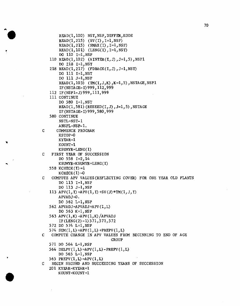
READ(1,100) NST,NSP,DIFFER,KODEREAD(1,215) (SV(I), I=l,NSP)READ(1,215) (SMAX (I) ,1=1, NSP)READ(1,101) (LENG(I), 1=1, NST)DO 110 1=1, NSP

110 READ(1,102) (AINTER(I, J) ,J=1,5), NSp1DO 218 I=l,NST

218 READ(1,217) (FDBACK(I,J),J=l,NST)DO 111 1=1, NSTDO 111 J=l, NSPREAD(1,103) ('IM(I, J ,K) ,K=1,5) , NSTAGE, NSP1IF (NSTAGE-I) 999, 112,999

112 IF(NSP1-J)999,lll,999111 CONTINUE

DO 580 I=l,NSTREAD(1,581) (RESEED(I,J),J=1,5),NSTAGEIF (NSTAGE-I) 999,580,999

580 CONTINUENSTL=NST-1ANSPL=NSP-1.

C COMMENCE PROGRAMKSTOP=OKYEAR=lKOUNT=lKSUMYR=LENG( 1)

C FIRST YEAR OF SUCCESSIONDO 558 1=2,14KSUMYR=KSUMYR+LENG(I)

558 KCHECK(I)=lKCHECK(l) =0

C COMPUTE APV VALUES (REFLECTING COVER) FOR ONE YEAR OLD PLANTSDO 113 I=l,NSPDO 113 J=l,NSP

113 APV(l, I) =APV(l, I) +SV(J)*'IM(l,J, I)APVADJ=O.DO 562 L=l,NSP

562 APVADJ=APVADJ+APV (1, L)DO 563 K=l,NSP

563 APV(l,K)=APV(l,K)/APVADJIF (LENG(2) -1) 571, 571, 572

572 DO 574 L=l,NSP574 SUM(l, L) =APV (1, L) +PREPV (1, L)

C COMPUTE CHANGE IN APV VALUES FROM BEGINNING TO END OF AGEGROUP

571 DO 564 L=l,NSP564 DELPV(l,L)=APV(l,L)-PREPV(l,L)

DO 565 L=l,NSP565 PREPV(l,L)=APV(l,L)

C BEGIN SECOND AND SUCCEEDING YEARS OF SUCCESSION201 KYEAR=KYEAR+l

KOUNT=KOUNT+1

70

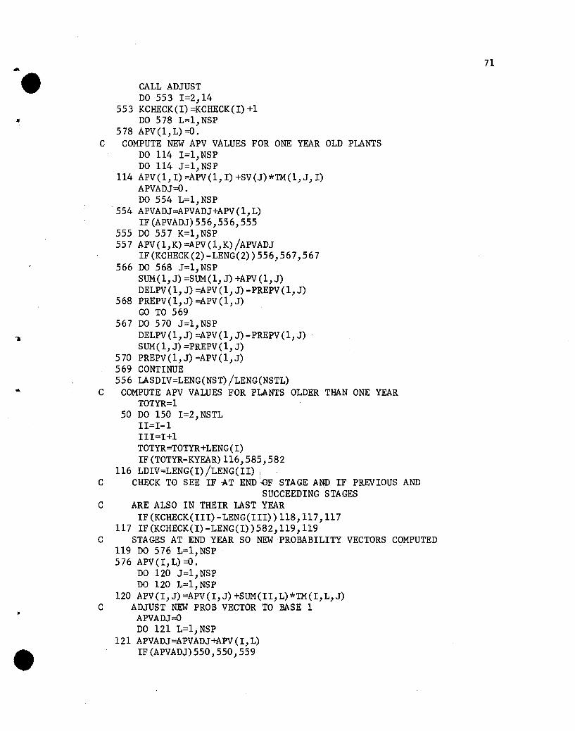
71~• CALL ADJUST

DO 553 1=2,14553 KCHECK(I)=KCHECK(I)+1

DO 578 L=l,NSP578 APV(l, L) =0.

C COMPUTE NEW APV VALUES FOR ONE YEAR OLD PLANTSDO 114 I=l,NSPDO 114 J=l,NSP

114 APV(l, I) =APV(l, I) +SV(J)*TM(l,J, I)APVADJ=O.DO 554 L=l,NSP

554 APVADJ=APVADJ+APV(l,L)IF (APVADJ) 556,556, 555

555 DO 557 K=l,NSP557 APV(l,K)=APV(l,K)/APVADJ

IF(KCHECK(2)-LENG(2))556,567,567566 DO 568 J=l,NSP

SUM(l, J) =SUM(l, J) +APV (1, J)DELPV(l,J)=APV(l,J)-PREPV(l,J)

568 PREPV(l,J)=APV(l,J)GO TO 569

567 DO 570 J=l,NSP11 DELPV (1, J) =APV (1, J) -PREPV (1, J) .

SUM( 1, J) =PREPV (1, J)570 PREPV (1, J) =APV(l, J)569 CONTINUE556 LASDIV=LENG(NST)/LENG(NSTL)

• C COMPUTE APV VALUES FOR PLANTS OLDER THAN ONE YEARTOTYR=l

50 DO 150 I=2,NSTLII=I-1III=I+1TOTYR=TOTYR+LENG(I)IF (TOTYR-KYEAR) 116,585,582

116 LDIV=LENG(I) /LENG(II) !

C CHECK TO SEE IF -AT END..QF STAGE AND IF PREVIOUS ANDSUCCEEDING STAGES

C ARE ALSO IN THEIR LAST YEARIF (KCHECK(III) -LENG(III)) 118,117,117

117 IF (KCHECK(I) -LENG(I)) 582,119,119C STAGES AT END YEAR SO NEW PROBABILITY VECTORS COMPUTED

119 DO 576 L=l,NSP576 APV(I,L) =0.

DO 120 J=l, NSPDO 120 L=l,NSP

120 APV (I, J) =APV (I, J) +SUM(II, L) *TM(I, L, J)C ADJUST NEW PROB VECTOR TO BASE 1

APVADJ=ODO 121 L=l,NSP

121 APVADJ=APVADJ+APV(I,L)

• IF (APVADJ) 550, 550, 559

..••

-"

•

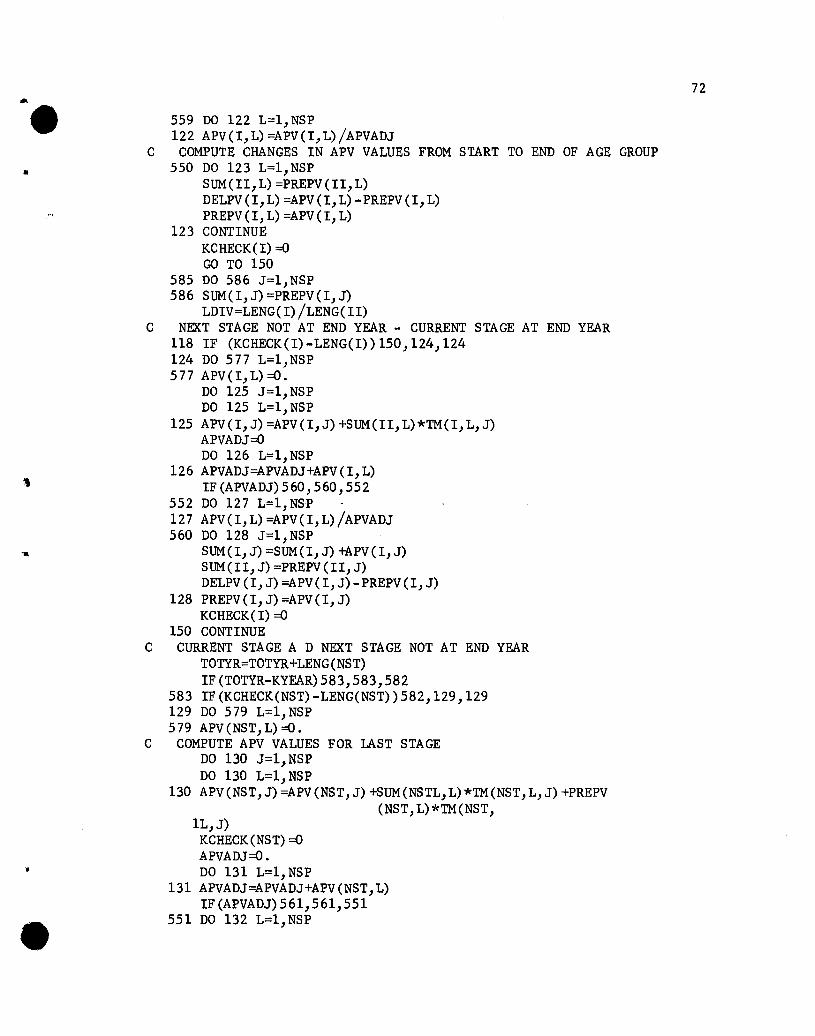
559 DO 122 L=l,NSP122 APV(I,L)=APV(I,L)/APVADJ

C COMPUTE CHANGES IN APV VALUES FROM START TO END OF AGE GROUP550 DO 123 L=l,NSP

SUM(II,L)=PREPV(II,L)DELPV(I,L)=APV(I,L)-PREPV(I,L)PREPV(I, L) =APV(I, L)

123 CONTINUEKCHECK (I) =0GO TO 150

585 DO 586 J=l,NSP586 SUM( I, J) =PREPV (I, J)

LDIV=LENG( I) /LENG( II)C NEXT STAGE NOT AT END YEAR - CURRENT STAGE AT END YEAR

118 IF (KCHECK(I)-LENG(I))150,124,124124 DO 577 L=l,NSP577 APV(I,L)=0.

DO 125 J=l, NSPDO 125 L=l,NSP

125 APV(I, J) =APV(I,J) +SUM(II, L)*TM(I, L, J)APVADJ=0DO 126 L=l,NSP

126 APVADJ=APVADJ+APV(I,L)IF (APVADJ) 560, 560,552

552 DO 127 L=l,NSP127 APV(I,L)=APV(I,L)/APVADJ560 DO 128 J=l,NSP

SUM(I, J) =SUM(I, J) +APV (I, J)SUM(II,J)=PREPV(II,J)DELPV(I,J)=APV(I,J)-PREPV(I,J)

128 PREPV(I,J)=APV(I,J)KCHECK( I) =0

150 CONTINUEC CURRENT STAGE A D NEXT STAGE NOT AT END YEAR

TOTYR=TOTYR+LENG(NST)IF (TOTYR-KYEAR)583,583,582

583 IF(KCHECK(NST)-LENG(NST))582,129,129129 DO 579 L=l,NSP579 APV(NST,L)=O.

C COMPUTE APV VALUES FOR LAST STAGEDO 130 J=l,NSPDO 130 L=l, NSP

130 APV(NST,J)=APV(NST,J)+SUM(NSTL,L)*TM(NST,L,J)+PREPV(NST,L)*TM(NST,

1L,J)KCHECK(NST)=0APVADJ=O.DO 131 L=l,NSP

131 APVADJ=APVADJ+APV(NST,L)IF(APVADJ)561,561,551

551 DO 132 L=l,NSP

72

..•..

..

•

132 APV(NST,L)=APV(NST,L)/APVADJ561 DO 133 L=l,NSP

SUM(NSTL,L)=PREPV(NSTL,L)DELPV(NST,L)=APV(NST,L)-PREPV(NST,L)

133 PREPV(NST,L)=APV(NST,L)582 IF(KSUMYR-KYEAR)587,587,588S88 KSTOP=OS87 IF(KYEAR-150)134,13S,139

C CHECK PRINT INTERVAL CODE(KODE)134 GO TO(136,137,138,139),KODE136 IF(KOUNT-10)221,140,221137 IF(KOUNT-20)221,140,221138 IF(KOUNT-2)221,140,221139 IF(KOUNT-SO)221,140,221135 KODE=4221 KSTOP=KSTOP+1

DO 141 I=l,NSTC CHECK TO SEE IF STABILIZED

DO 141 J=l,NSPIF (ABS (DELPV (I, J)) -DIFFER) 142,142,143

142 CONTINUE141 CONTINUE

GO TO(144,140),KSTOP143 KSTOP =0144 ATEST=!. O*KYEAR/SO ..

IF (KYEAR/50-ATEST) 201,140,201C BEGIN OUTPUT OF INFORMATION

140 WRITE(3,401) KYEARWRITE(3,402) (SV(L),L=1,NSP)WRITE(3,407)DO 146 I=l,NST

146 WRITE(3,403) I,(APV(I,J),J=l,NSP)KOUNT=OIF (KYEAR-1000) 733,147,147

733 IF(KSTOP-2)201,147,147147 WRITE(3,404)

DO 148 I=1,NSTWRITE(3,408) IDO 160 J=l,NSP

160 WRITE(3,40S) I,J,(TM(I,J,K), K=l,NSP)148 WRITE(3,406)

READ(1,105) AMOREIF (AMORE) 149,149,202

S81 FO~T(SFS.2,3X,I2)

100 FORMAT(212,6X,F10.8,9X,I1)101 FORMAT(14(3X,I2))102 FORMAT(SFS.0,4X,I1)103 FORMAT(SF10.8,8X,I2,9X,I1)105 FORMAT(Il)

99 FORMAT(15X,IS)215 FORMAT(lOX,5FlO. 8)

73

..•

•

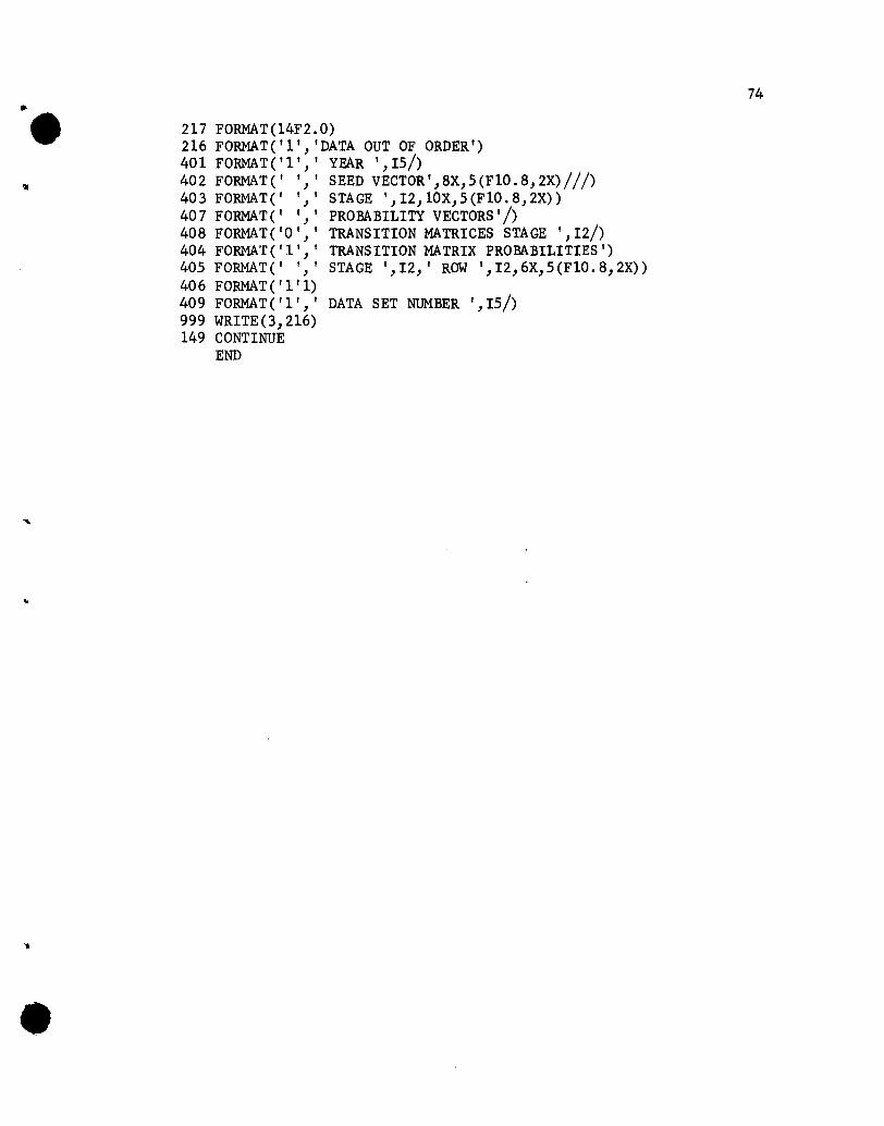
217 FORMAT(14F2.0)216 FORMAT('1', 'DATA OUT OF ORDER')401 FORMAT (' l' " YEAR ',15/)402 FORMAT(' ',' SEED VECTOR',8X,5(F10.8,2X)///)403 FORMAT(' ',' STAGE ',I2,lOX,5(F10.8,2X))407 FORMAT(' ',' PROBABILITY VECTORS'/)408 FORMAT('O',' TRANSITION MATRICES STAGE ',12/)404 FORMAT('l',' TRANSITION MATRIX PROBABILITIES')405 FORMAT(' ',' STAGE ',12,' ROW ',I2,6X,5(FlO.8,2X))406 FORMAT ( '1'1)409 FORMAT('l',' DATA SET NUMBER ',15/)999 WRITE(3,216)149 CONTINUE

END

74

•

•

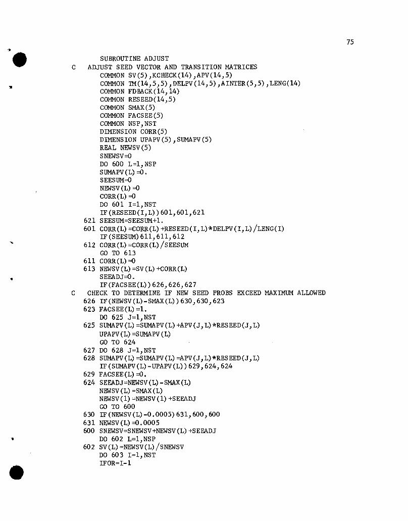
SUBROUTINE ADJUSTC ADJUST SEED VECTOR AND TRANSITION MATRICES

COMMON SV(5),KCHECK(14),APV(14,5)COMMON TM(14,5,5),DELPV(14,5),AINTER(5,5),LENG(14)COMMON FDBACK(14,14)COMMON RESEED(14,5)COMMON SMAX(5)COMMON FACSEE(5)COMMON NSP,NSTDIMENSION CORR(5)DIMENSION UPAPV(5),SUMAPV(5)REAL NEWSV(5)SNEWSV=ODO 600 L=l,NSPSUMAPV (L) =0.SEESUM=ONEWSV(L)=0CORR(L)=0DO 601 I=l,NSTIF(RESEED(I,L»601,601,621

621 SEESUM=SEESUM+1.601 CORR(L)=CORR(L)+RESEED(I,L)*DELPV(I,L)/LENG(I)

IF(SEESUM)611,611,612612 CORR(L)=CORR(L)/SEESUM

GO TO 613611 CORR(L) =0613 NEWSV(L)=SV(L)+CORR(L)

SEEADJ=O .IF (FACSEE(L»626,626,627

C CHECK TO DETERMINE IF NEW SEED PROBS EXCEED MAXIMUM ALLOWED626 IF(NEWSV(L)-SMAX(L»630,630,623623 FACSEE(L) =1-

DO 625 J=l,NST625 SUMAPV(L)=SUMAPV(L)+APV(J,L)*RESEED(J,L)

UPAPV (L) =SUMAPV (L)GO TO 624

627 DO 628 J=l,NST628 SUMAPV(L)=SUMAPV(L)=APV(J,L)*RESEED(J,L)

IF (SUMAPV(L)-UPAPV(L»629,624, 624629 FACSEE(L)=0.624 SEEADJ=NEWSV(L)-SMAX(L)

NEWSV (L) =SMAX (L)NEWSV(l)=NEWSV(l)+SEEADJGO TO 600

630 IF(NEWSV(L)-0.0005)631,600,600631 NEWSV(L)=O.0005600 SNEWSV=SNEWSV+NEWSV(L)+SEEADJ

DO 602 L=l,NSP602 SV(L)=NEWSV(L)/SNEWSV

DO 603 I=l,NSTIFOR=I-1

75

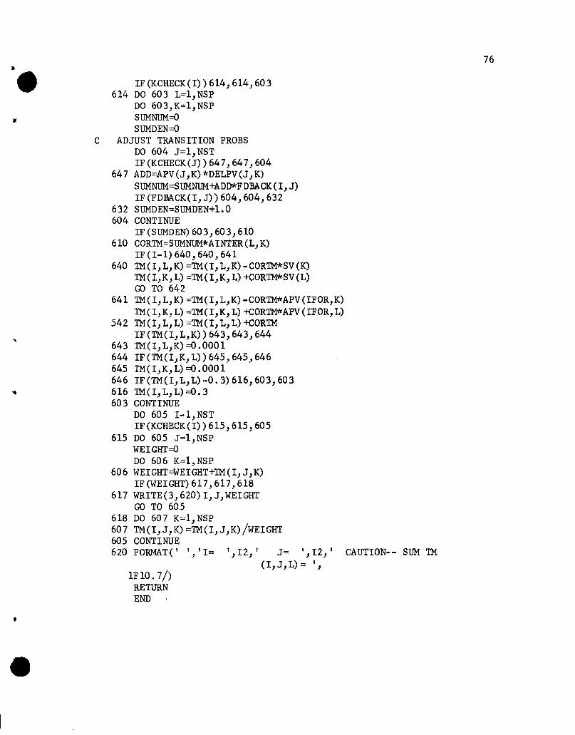
76

CAUTION-- SUM TM

1FlO. 7/)RETURNEND

IF(KCHECK(I»614,614,603614 DO 603 L=1,NSP

DO 603,K=1,NSPSUMNUM=OSUMDEN=O

ADJUST TRANSITION PROBSDO 604 J=1,NSTIF(KCHECK(J»647, 647, 604

647 ADD=APV(J,K)*DELPV(J,K)SUMNUM=SUMNUM+ADD*FDBACK(I,J)IF (FDBACK(I,J»604, 604, 632

632 SUMDEN=SUMDEN+1.0604 CONTINUE

IF (SUMDEN) 603,603,610610 CORTM=SUMNUM*AINTER(L,K)

IF(I-1) 640,640,641640 TM(I,L,K)=TM(I,L,K)-CORTM*SV(K)

TM(I,K,L) =TM(I,K,L) +CORTM*SV(L)GO TO 642

641 TM(I,L,K)=TM(I,L,K)-CORTM*APV(IFOR,K)TM(I,K, L) =TM(I,K, L) +CORTM*APV (IFOR, L)

542 TM(I,L,L)=TM(I,L,L)+CORTMIF(TM(I,L,K»643,643,644

643 TM(I,L,K)=O.OOOI644 IF(TM(I,K,L»645,645,646645 TM(I,K,L)=O.0001646 IF(TM(I,L,L)-0.3)616,603,603616 TM(I,L,L)=O.3603 CONTINUE

DO 605 1-1, NSTIF(KCHECK(I»615,615,605

615 DO 605 J=1,NSPWEIGHT=ODO 606 K=1,NSP

606 WEIGHT=WEIGHT+TM(I,J,K)IF (WEIGHT) 617,617,618

617 WRITE(3,620)I,J,WEIGHTGO TO 605

618 DO 607 K=1,NSP607 TM(I,J,K)=TM(I,J,K)/WEIGHT605 CONTINUE620 FORMAT(' ','1= ',12,' J= ',12,'

(I, J, L) = "

C

•

-.•

•

•

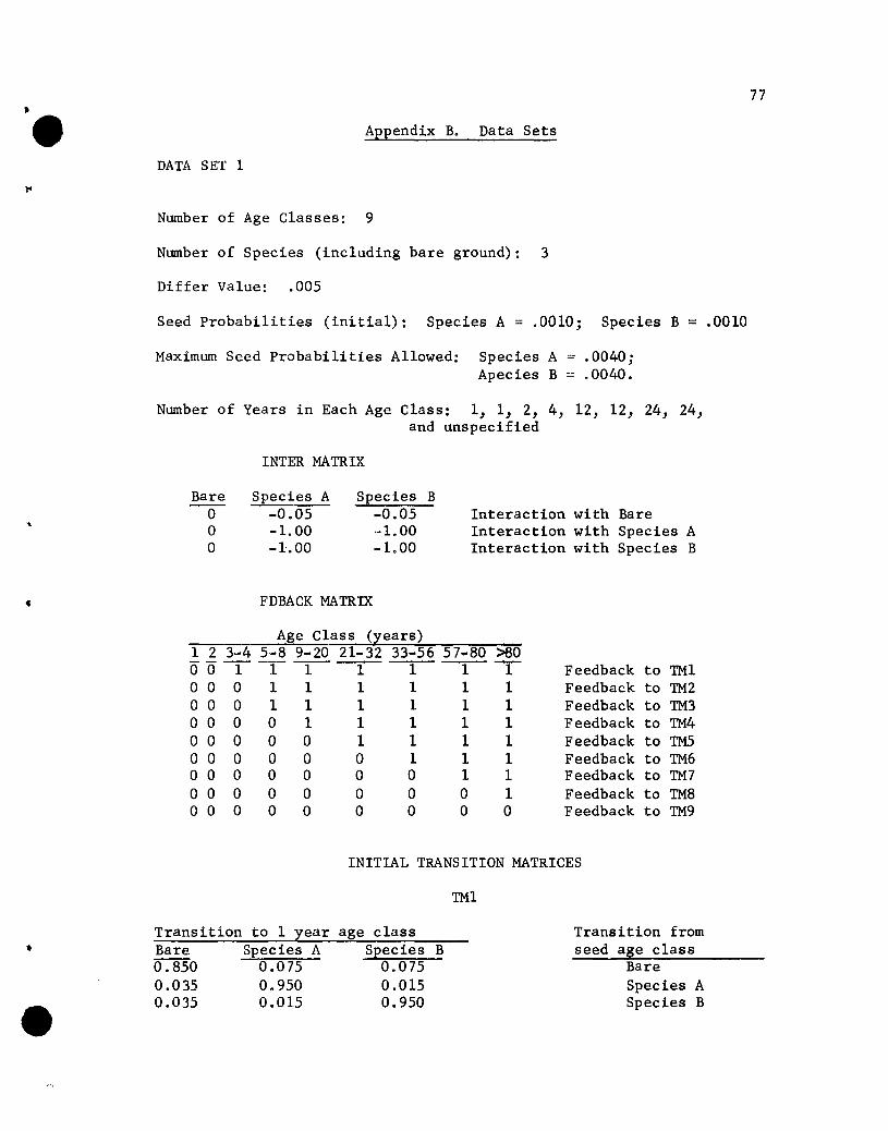
..• Appendix B. Data Sets

DATA SET 1

Number of Age Classes: 9

Number of Species (including bare ground): 3

Differ Value: .005

Seed Probabilities (initial): Species A = .0010; Species B = .0010

77

Maximum Seed Probabilities Allowed: Species AApecies B

= .0040 j

.0040.

Number of Years in Each Age Class: 1, 1, 2, 4, 12, 12, 24, 24,and unspecified

INTER MATRIX

Bareooo

Species A-0.05-1.00-1-.00

Species B-0.05-1.00-LaO

Interaction with BareInteraction with Species AInteraction with Species B

FDBACK MATRIX

Age Class (years)1 2 3~4 5-8 9-20 21-32 33-56 57-80 >6000-1--1--1- 1 1 1 T00011111100011111100001 1 11100000111100000 0 11100000001100000 0 0 0 1000000000

Feedback to TM1Feedback to TM2Feedback to TM3Feedback to TM4Feedback to TM5Feedback to TM6Feedback to TM7Feedback to TM8Feedback to TM9

INITIAL TRANSITION MATRICES

TM1

•

•Transition to 1 yearBare Species A0.850 0.0750.035 0.9500.035 0.015

age classSpecies B

0.0750.0150.950

Transition fromseed age class

BareSpecies ASpecies B

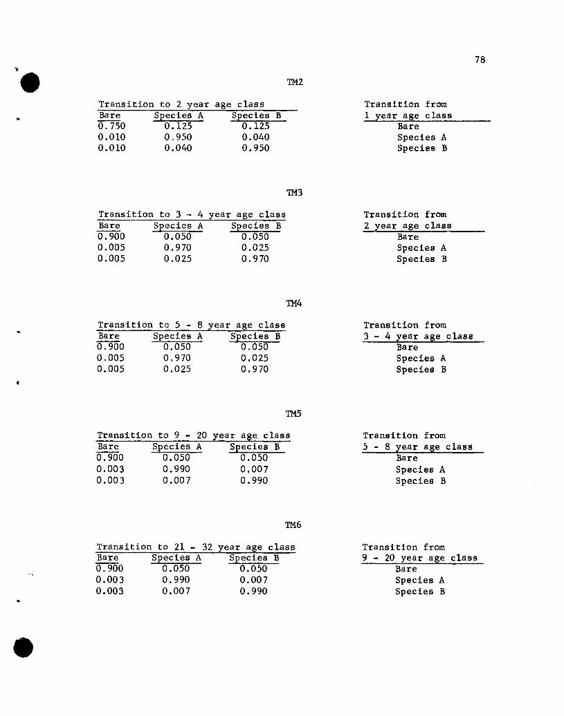
Transition to 2 yearBare Species A0.750 0.1250.010 0.9500.010 0.040

age classSpecies B

0.1250.0400.950

TM2

TM3

78

Transition from1 year age class

BareSpecies ASpecies B

Transition to 3 -Bare Species0.900 0.0500.005 0.9700.005 0.025

4 year age classA Species B

0.0500.0250.970

Transition from2 year age class

BareSpecies ASpecies B

TM4

Transition to 5 - 8 year age class Transition fromBare Species A Species B 3 - 4 year age class0.900 0.050 0.050 Bare0.005 0.970 0.025 Species A0.005 0.025 0.970 Species B

•

TM5

Transition to 9 - 20 year age class Transition fromBare Species A Species B 5 - 8 year age class0.900 0.050 0.050 Bare0.003 0.990 0.007 Species A0.003 0.007 0.990 Species B

TM6

..

•

Transition to 21 - 32Bare Species A0.900 0.0500.003 0.9900.003 0.007

year age classSpecies B

0.0500.0070.990

Transition from9 - 20 year age

BareSpecies ASpecies B

class

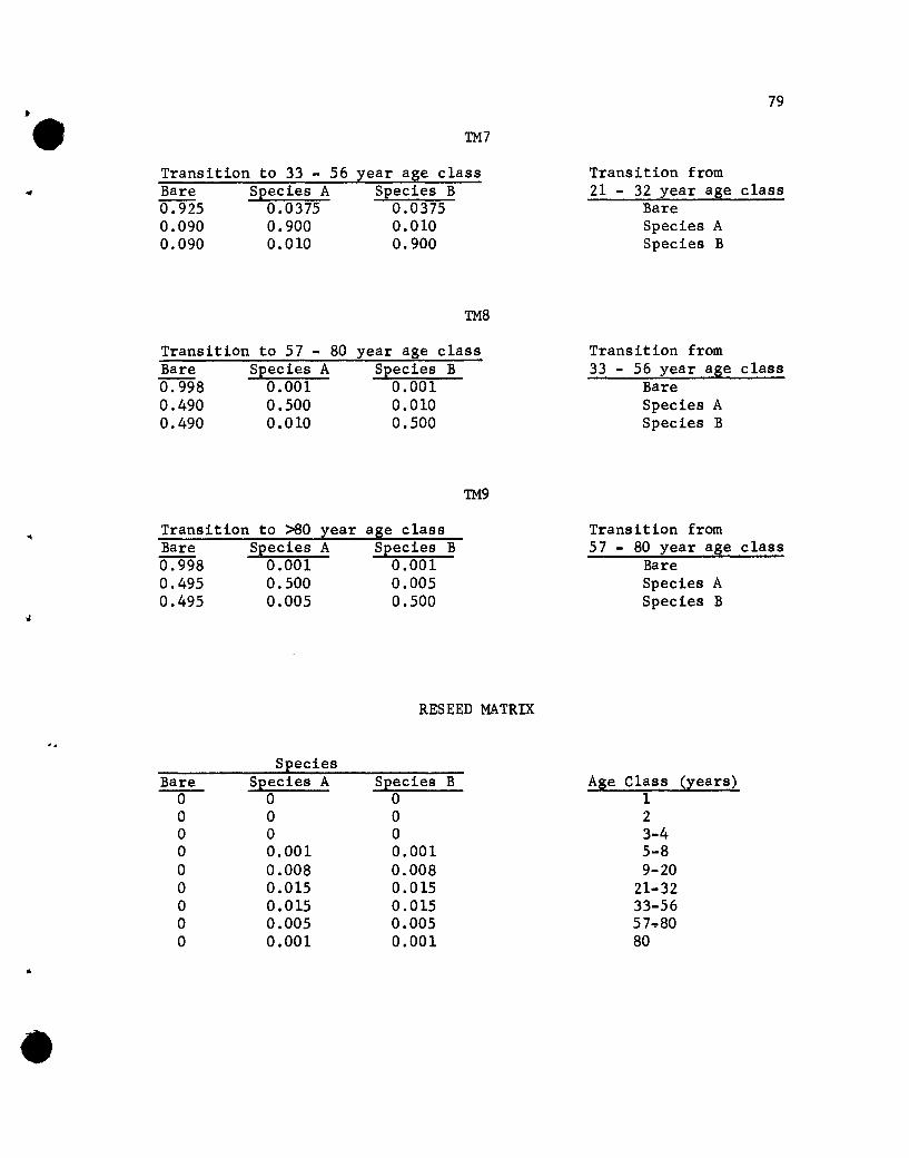
..• TM7

Transition to 33 - 56 year age classBare Species A Species B0.925 0.0375 0.03750.090 0.900 0.0100.090 0.010 0.900

TM8

79

Transition from21 - 32 year age class

BareSpecies ASpecies B

Transition to 57 - 80Bare Species A0.998 0.0010.490 0.5000.490 0.010

year age classSpecies B

0.0010.0100.500

TM9

Transition from33 - 56 year age class

BareSpecies ASpecies B

Transition to >80 yearBare Species A0.998 0.0010.495 0.5000.495 0.005

age classSpecies B

0.0010.0050.500

Transition from57 - 80 year age

BareSpecies ASpecies B

class

RES EED MATRIX

-.Species

Bare Species A Species B Age Class (years)-0- 0 0 1

0 0 0 20 0 0 3-40 0.001 0.001 5-80 0.008 0.008 9-200 0.015 0.015 21-320 0.015 0.015 33-560 0.005 0.005 57... 800 0.001 0.001 80

..

•

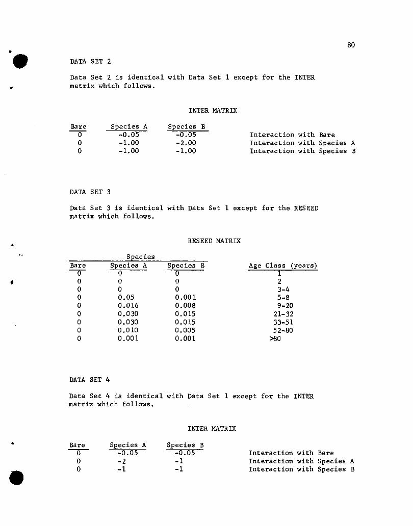
..•80

DATA SET 2

Data Set 2 is identical with Data Set 1 except for the INTERmatrix which follows.

INTER MATRIX

Bare-0-

oo

Species A-0.05-1.00-1.00

Species B-0.05-2.00-1.00

Interaction with BareInteraction with Species AInteraction with Species B

-,-

f

DATA SET 3

Data Set 3 is identical with Data Set 1 except for the RESEEDmatrix which follows.

RESEED MATRIX

SpeciesBare Species A Species B Age Class (years)() 0 0 1

0 0 0 20 0 0 3-40 0.05 0.001 5-80 0.016 0.008 9-200 0.030 0.015 21-320 0.030 0.015 33-510 O.OlD 0.005 52-800 0.001 0.001 >80

DATA SET 4

Data Set 4 is identical with Data Set 1 except for the INTERmatrix which follows.

INTER MATRIX

•

•Bare

ooo

Species A-0.05-2-1

Species B-0.05-1-1

Interaction with BareInteraction with Species AInteraction with Species B

~.

•

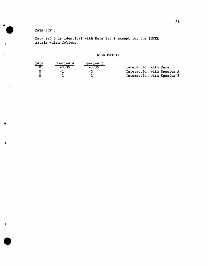
81

DATA SET 5

Data Set 5 is identical with Data Set 1 except for the INTERmatrix which follows •

INTER MATRIX

'·.4

to

•

Bare---0

oo

Species A-0.05-1-1

Species B-0.05-3-1

Interaction with BareInteraction with Species AInteraction with Species B

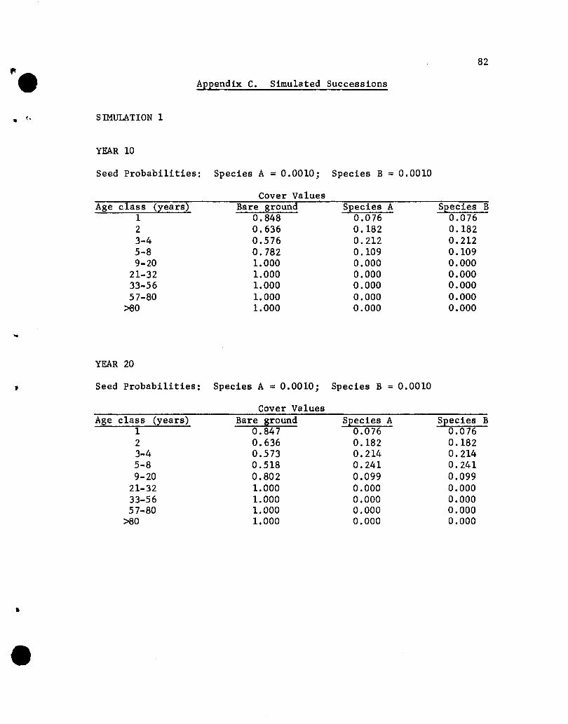
82

~. Appendix C. Simulated Successions

• ~-~ SIMULATION 1

YEAR 10

Seed Probabilities: Species A = 0.0010 j Species B = 0.0010

Cover ValuesAge class (years) Bare ground Species A Species B

1 0.848 0.076 0.0762 0.636 0.182 0.1823-4 0.576 0.212 0.2125-8 0.782 0.109 0.1099-20 1.000 0.000 0.000

21-32 1.000 0.000 0.00033-56 1.000 0.000 0.00057-80 1.000 0.000 0.000

>80 1.000 0.000 0.000

..YEAR 20

Seed Probabilities: Species A = 0.0010j Species B = 0.0010

Cover ValuesAge class (years) Bare ground Species A Species B

1 0.847 0.076 0.0762 0.636 0.182 0.1823-4 0.573 0.214 0.2145-8 0.518 0.241 0.2419-20 0.802 0.099 0.099

21-32 1.000 0.000 0.00033-56 1.000 0.000 0.00057-80 1.000 0.000 0.000

>80 1.000 0.000 0.000

•

•

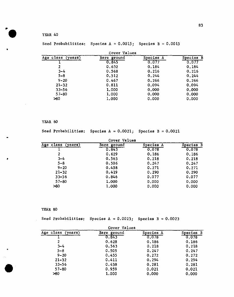
...YEAR 40

83

Seed Probabilities: Species A = 0.0015j Species B = 0.0015..

Age class (years)123-45-89-20

21-3233-5657-80

>60

Cover valuesBare ground

0.8450.6320.5680.5120.4670.8111.0001.0001.000

Species A0.0770.1840.2160.2440.2660.0940.0000.0000.000

Species B0.0770.1840.2160.2440.2660.0940.0000.0000.000

YEAR 60

Seed Probabilities: Species A = 0.0021j Species B = 0.0021

Cover ValuesAge class (years) Bare ground Species A Species B

1 0.843 0.078 0.0782 0.629 0.186 0.1863-4 0.563 0.218 0.2185-8 0.506 0.247 0.2479-20 0.458 0.271 0.271

21-32 0.419 0.290 0.29033-56 0.846 0.077 0.07757-80 1.000 0.000 0.000

>60 1.000 0.000 0.000

YEAR 80

Seed Probabilities: Species A = 0.0023j Species B = 0.0023

Cover ValuesAge class (years) Bare ground Species A Species B

1 0.843 0.078 0.0782 0.628 0.186 0.1863-4 0.563 0.218 0.2185-8 0.505 0.247 0.2479-20 0.455 0.272 0.272

21-32 0.411 0.294 0.294

• 33-56 0.438 0.281 0.28157-80 0.959 0.021 0.021

>60 1.000 0.000 0.000

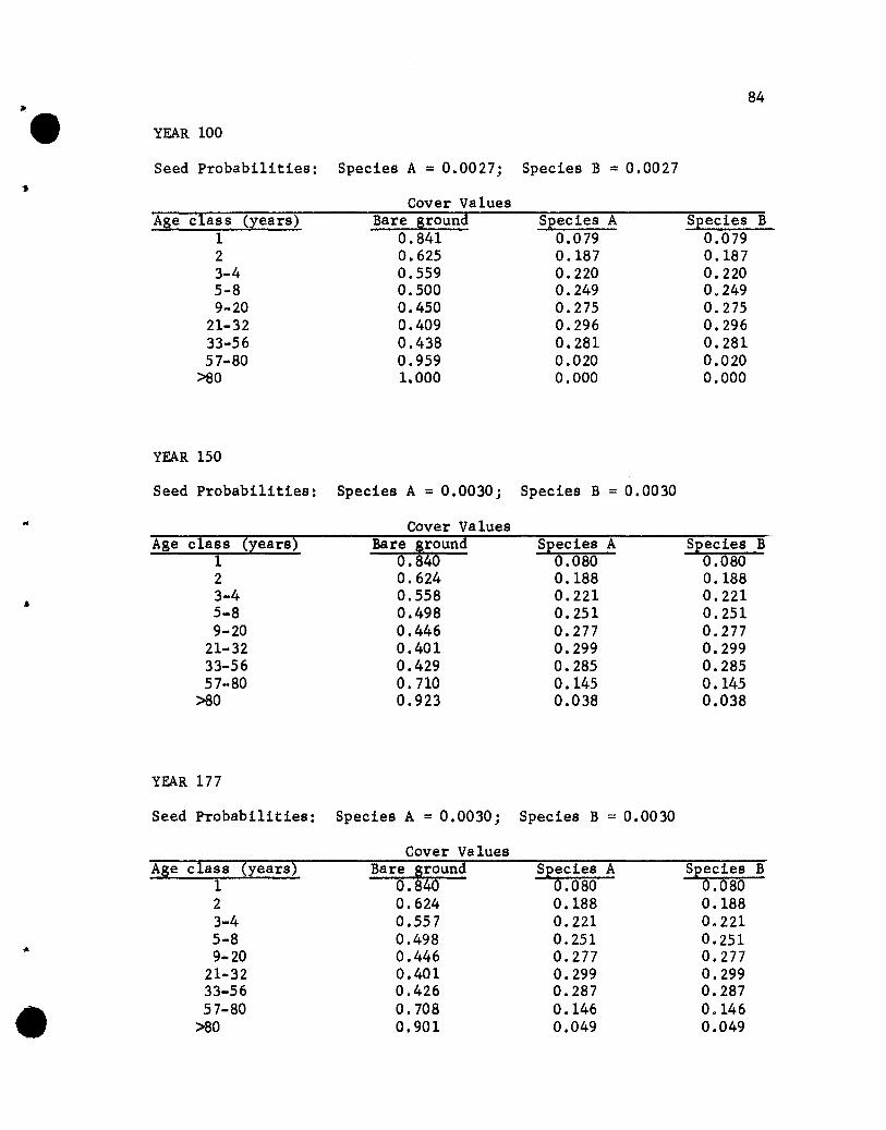
~.YEAR 100

Seed Probabilities: Species A = 0.0027; Species B = 0.0027

84

Age class (years)123-45-89-20

21-3233-5657-80

>80

Cover ValuesBare ground

0.8410.6250.5590.5000.4500.4090.4380.9591.000

Species A0.0790.1870.2200.2490.2750.2960.2810.0200.000

Species B0.0790.1870.2200.2490.2750.2960.2810.0200.000

YEAR 150

Seed Probabilities: Species A = 0.0030; Species B = 0.0030

.. Cover ValuesAge class (years) Bare ground Species A Species B

1 0.840 0.080 0.0802 0.624 0.188 0.188

,. 3-4 0.558 0.221 0.2215-8 0.498 0.251 0.2519-20 0.446 0.277 0.277

21-32 0.401 0.299 0.29933-56 0.429 0.285 0.28557-80 0.710 0.145 0.145

>80 0.923 0.038 0.038

YEAR 177

Seed Probabilities: Species A = 0.0030; Species B = 0.0030

Cover ValuesAge class (years) Bare ground Species A Species B

1 0.840 0.080 0.0802 0.624 0.188 0.1883-4 0.557 0.221 0.2215-8 0.498 0.251 0.2519-20 0.446 0.277 0.277

21-32 0.401 0.299 0.29933-56 0.426 0.287 0.287

• 57-80 0.708 0.146 0.146>80 0.901 0.049 0.049

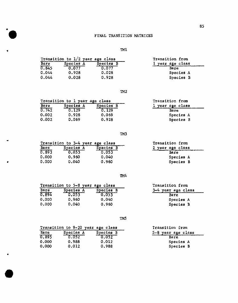
~.FINAL TRANSITION MATRICES

TM1

85

Transition to 1/2 year~ Species A0.845 0.0770.044 0.9280.044 0.028

age classSpecies B

0.0770.0280.928

Transition from1 year age class

BareSpecies ASpecies B

TM2

Transition to 1 year age classBare Species A Species B0.742 0.129 0.1290.002 0.928 0.0690.002 0.069 0.928

TM3..

Transition to 3-4 year age classBare Species A Species B0.893 0.053 0.0530.000 0.960 0.0400.000 0.040 0.960

TM4

Transition to 5-8 year age classBare Species A Species B0.894 0.053 0.0530.000 0.960 0.0400.000 0.040 0.960

TM5

Transition to 9-20 year age classBare Species A Species B0.895 0.052 0.0520.000 0.988 0.0120.000 0.012 0.988

•

Transition from1 year age class

BareSpecies ASpecies B

Transition from2 year age class

BareSpecies ASpecies B

Transition from3-4 year age class

BareSpecies ASpecies B

Transition from5-8 year age class

BareSpecies ASpecies B

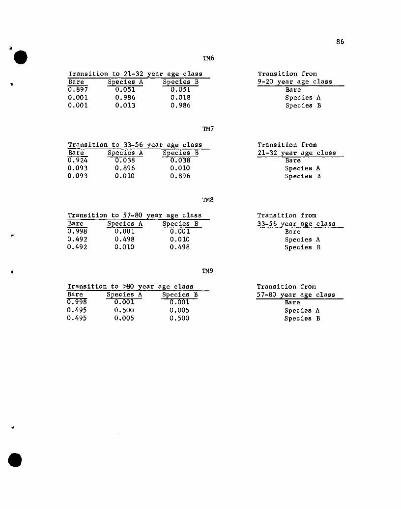
86

~. TM6

Transition to 21-32 year age class Transition fromBare Species A Species B 9-20 year age class0.897 0.051 0.051 Bare0.001 0.986 0.018 Species A0.001 0.013 0.986 Species B

TM7

Transition to 33-56 year age class Transition fromBare Species A Species B 21-32 year age class0.924 0.038 0.038 Bare0.093 0.896 0.010 Species A0.093 0.010 0.896 Species B

TM8

Transition to 57-80 year age class Transition fromBare Species A Species B 33-56 year age class0.998 0.001 0.001 Bare..0.492 0.498 0.010 Species A0.492 0.010 0.498 Species B

•

..

•

Transition to >80 yearBare Species A0.998 0.0010.495 0.5000.495 0.005

age classSpecies B

0.0010.0050.500

TM9

Transition from57-80 year age class

BareSpecies ASpecies B

~. SIMUlATION 2

YEAR 10

Seed Probabilities: Species A = O.OOlj Species B = 0.001

87

Age class (years)123-45-89-JO

21-3233-5657-80

>80

Cover ValuesBare ground

0.8480.6370.5750.7831.0001.0001.0001.0001.000

Species A0.0760.1810.2120.1090.0000.0000.0000.0000.000

Species B0.0760.1820.2130.1090.0000.0000.0000.0000.000

YEAR 20

Seed Probabilities: Species A = O.OOlj Species B = 0.001

Cover ValuesAge class (years) Bare ground Species A Species B

1 0.847 0.076 0.076

• 2 0.636 0.181 0.1833-4 0.573 0.209 0.2185-8 0.518 0.237 0.2459-20 0.803 0.099 0.099

21-32 1.000 0.000 0.00033-56 1.000 0.000 0.00057-80 1.000 0.000 0.000

>80 1.000 0.000 0.000

YEAR 40

Seed Probabilities: Species A = 0.0015j Species B = 0.0015

Cover ValuesAge class (years) Bare ground Species A Species B

1 0.845 0.077 0.0772 0.633 0.181 0.1863-4 0.568 0.204 0.2285-8 0.512 0.225 0.2639-20 0.467 0.262 0.271

21-32 0.811 0.094 0.094

• 33-56 1.000 0.000 0.00057-80 1.000 0.000 0.000

>80 1.000 0.000 0.000

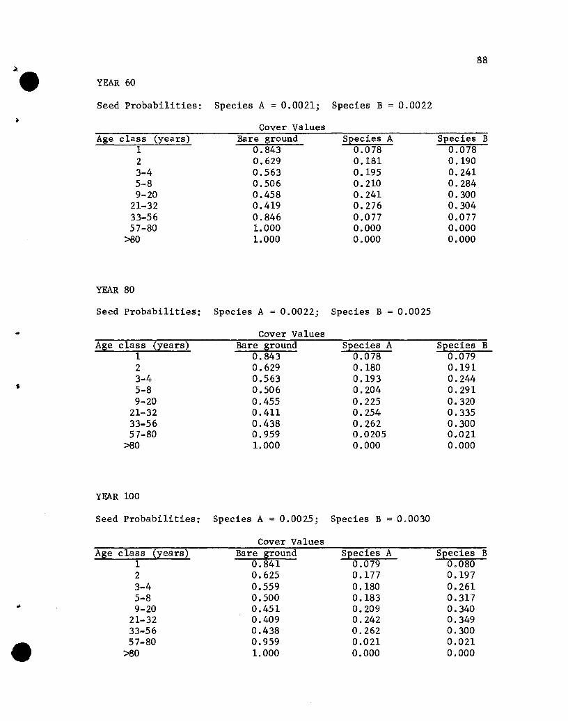
~. YEAR 60

Seed Probabilities: Species A = 0.0021; Species B = 0.0022

88

Age class (years)123-45-89-20

21-3233-5657-80

>80

Cover ValuesBare ground

0.8430.6290.5630.5060.4580.4190.8461.0001.000

Species A0.0780.1810.1950.2100.2410.2760.0770.0000.000

Species B0.0780.1900.2410.2840.3000.3040.0770.0000.000

YEAR 80

Seed Probabilities: Species A = 0.0022; Species B = 0.0025

Cover ValuesAge class (years) Bare ground Species A Species B

1 0.843 0.078 0.0792 0.629 0.180 0.1913-4 0.563 0.193 0.244

• 5-8 0.506 0.204 0.2919-20 0.455 0.225 0.320

21-32 0.411 0.254 0.33533-56 0.438 0.262 0.30057-80 0.959 0.0205 0.021

>80 1.000 0.000 0.000

YEAR 100

Seed Probabilities: Species A = 0.0025; Species B = 0.0030

•

Age class (years)123-45... 89-20

21-3233-5657-80

>80

Cover ValuesBare ground

0.8410.6250.5590.5000.4510.4090.4380.9591.000

Species A0.0790.1770.1800.1830.2090.2420.2620.0210.000

Species B0.0800.1970.2610.3170.3400.3490.3000.0210.000

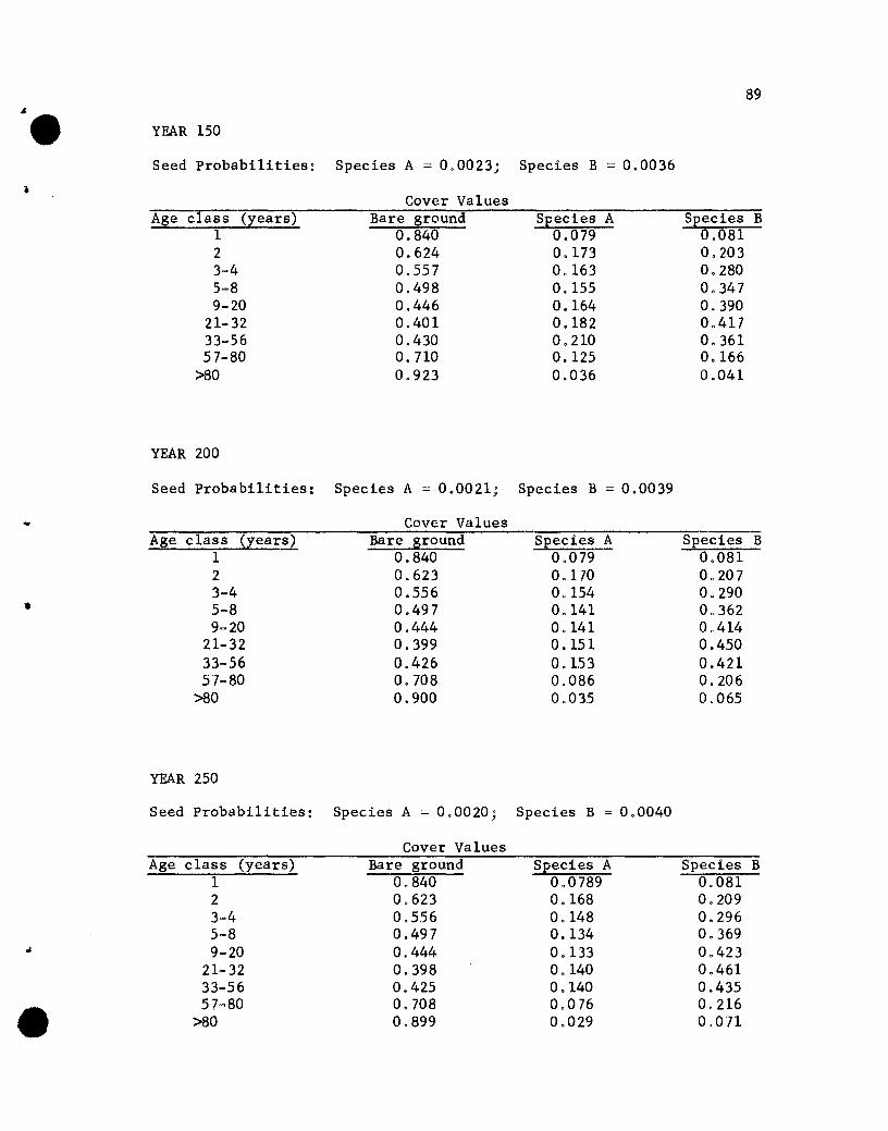
~. YEAR 150

Seed Probabilities: Species A = 0.0023; Species B = 0.0036

89

l

Age class (years)123-45-89-20

21-3233-5657-80

>80

Cover ValuesBare ground

0.8400.6240.5570.4980.4460.4010.430O. 7100.923

Species A0.0790.1730.1630.1550.1640.1820.2100.1250.036

Species B0.0810.2030.2800.3470.3900.4170.3610.1660.041

YEAR 200

Seed Probabilities: Species A = 0.0021; Species B = 0.0039

Cover ValuesAge class (years) Bare ground Species A Species B

1 0.840 0.079 0.0812 0.623 0.170 0.2073-4 0.556 0.154 0.290

• 5-8 0.497 0.141 0.3629-20 0.444 0.141 0.414

21-32 0.399 0.151 0.45033-56 0.426 0.153 0.42157-80 0.708 0.086 0.206

>80 0.900 0.035 0.065

YEAR 250

Seed Probabilities: Species A = 0.0020; Species B = 0.0040

•

Age class (years)123-45-89-20

21-3233-5657-80

>80

Cover ValuesBare ground

0.8400.6230.5560.4970.4440.3980.4250.7080.899

Species A0.07890.1680.1480.1340.1330.1400.1400.0760.029

Species B0.0810.2090.2960.3690.4230.4610.4350.2160.071

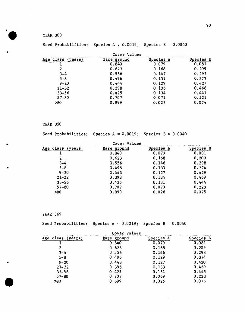
~. YEAR 300

Seed Probabilities: Species A . 0.0019; Species B = 0.0040

90

Species B0.0810.2090.2970.3730.4270.4660.4410.2210.074

Species A0.0790.1680.1470.1310.1290.1360.1340.0720.027

Cover ValuesBare ground

0.8400.6230.5560.4960.4440.3980.4250.7070.899

123-45-89-20

21-3233-5657-80

>80

class (years)Age

YEAR 350

Seed Probabilities: Species A =0.0019; Species B =0.0040

Cover ValuesAge class (years) Bare ground Species A Species B

1 0.840 0.079 0.0812 0.623 0.168 0.2093-4 0.556 0.146 0.2985-8 0.496 0.130 0.3749-20 0.443 O. 127 0.429

21-32 0.398 0.134 0.46933..56 0.425 0.131 0.44457-80 0.707 0.070 0.223

>80 0.899 0.026 0.075

YEAR 369

Seed Probabilities: Species A = 0.0019; Species B = 0.0040

•

Age class (years)123-45-89-20

21-3233-5657-80

>80

Cover ValuesBare ground

0.8400.6230.5560.4960.4430.3980.4250.7070.899

Species A0.0790.1680.1460.1290.1270.1330.1310.0690.025

Species B0.0810.2090.2980.3740.4300.4690.4450.2230.076

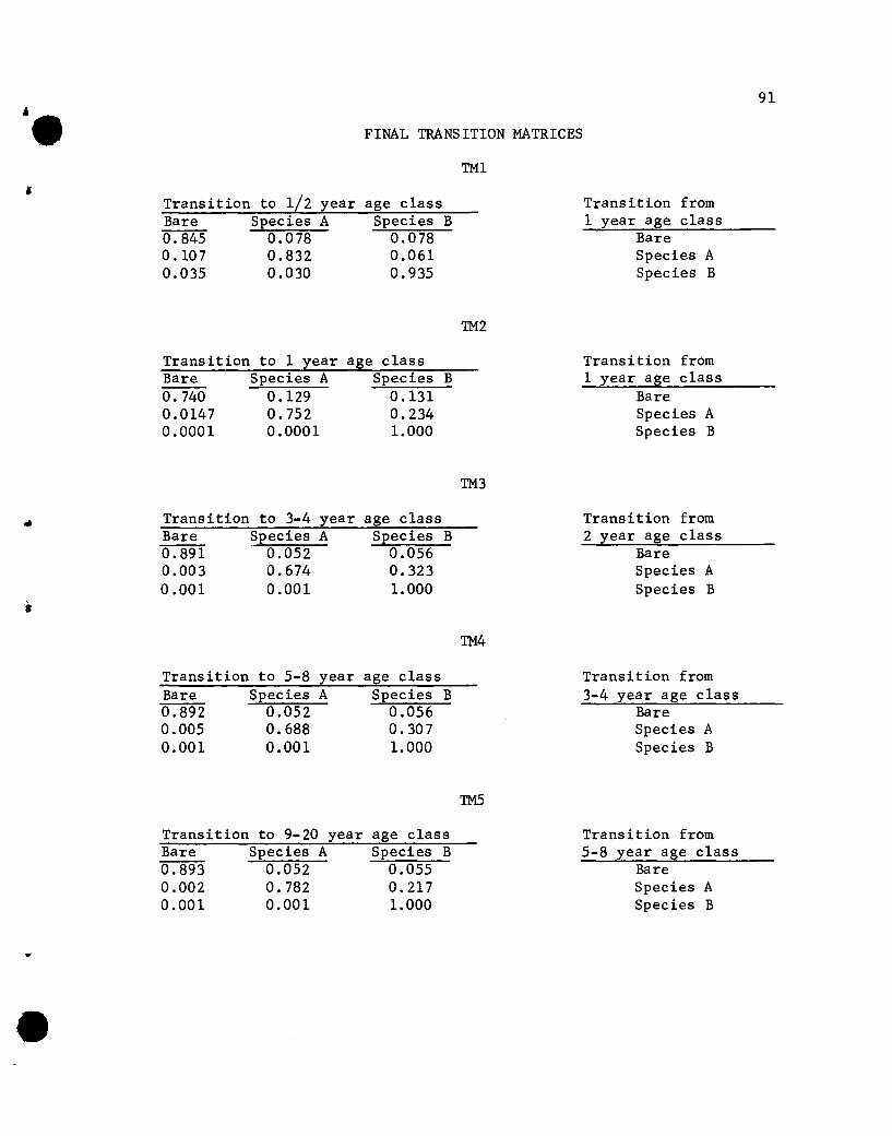
FINAL TRANSITION MATRICES

TM1

91

Transition to 1/2 yearBare Species A0.845 0.0780.107 0.8320.035 0.030

age classSpecies B

0.0780.0610.935

TM2

Transition from1 year age class

BareSpecies ASpecies B

Transition to 1 yearBare Species A0.740 0.1290.0147 0.7520.0001 0.0001

age classSpecies B

0.1310.2341.000

TM3

Transition from1 year age class

BareSpecies ASpecies B

Transition to 3-4 yearBare Species A0.891 0.0520.003 0.6740.001 0.001

Transition to 5-8 yearBare Species A0.892 0.0520.005 0.6880.001 0.001

age classSpecies B

0.0560.3231.000

age classSpecies B

0.0560.3071.000

TM4

TM5

Transition from2 year age class

BareSpecies ASpecies B

Transition from3-4 year age class

BareSpecies ASpecies B

•

Transition to 9-20 yearBare Species A0.893 0.0520.002 0.7820.001 0.001

age classSpecies B

0.0550.2171.000

Transition from5-8 year age class

BareSpecies ASpecies B

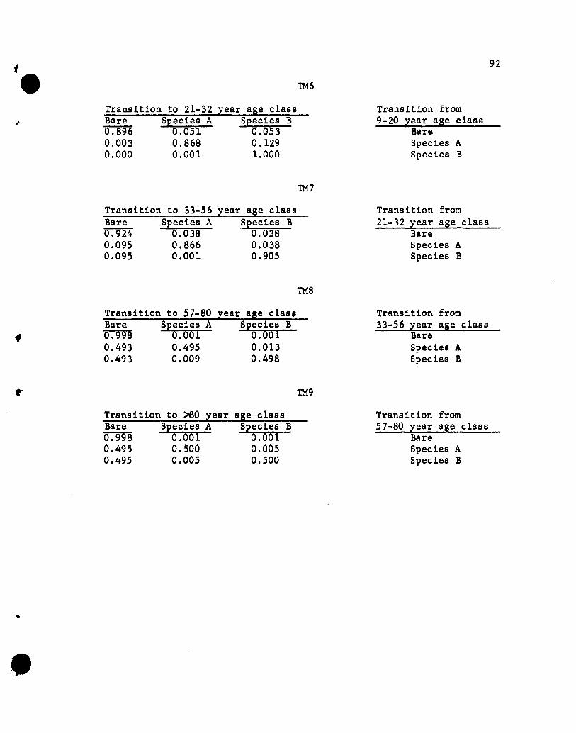
t• Transition to 21-32Bare Species A0.896 0.0510.003 0.8680.000 0.001

'!M6

year age classSpecies B

0.0530.1291.000

'!M7

Transition from9-20 year age class

BareSpecies ASpecies B

92

Transition to 33-56 year age classBare Species A Species B0.924 0.038 0.0380.095 0.866 0.0380.095 0.001 0.905

'!M8

Transition to 57-80 year age classBare Species A Species B0.998 0.001 0.0010.493 0.495 0.0130.493 0.009 0.498

'!M9

Transition from21-32 year age class

BareSpecies ASpecies B

Transition from33-56 year age class

BareSpecies ASpecies B

,.'

•

Transition to >80 yearBare Species A0.998 0.0010.495 0.5000.495 0.005

age classSpecies B

0.0010.0050.500

Transition from57-80 year age class

BareSpecies ASpecies B

'.i

SIMULATION 3

YEAR 10

Seed Probabilities: Species A = 0.0015; Species B = 0.0010

93

Age class (years)123-45-89-20

21-3233-5657-80

>80

YEAR 20

Cover ValuesBare ground

0.8470.6370.5750.7831.0001.0001.0001.0001.000

Species A0.0770.1820.2120.1090.0000.0000.0000.0000.000

Species B0.0760.1820.2120.1090.0000.0000.0000.0000.000

Seed Probabilities: Species A = 0.0030; Species B = 0.0010

Age class (years)123-45-89-20

21-3233-5657-80

>80

Cover ValuesBare ground

0.8460.6340.5720.5170.8031.0001.0001.0001.000

Species A0.0780.1840.2150.2420.0990.0000.0000.0000.000

Species B0.0760.1820.2130.2410.0990.0000.0000.0000.000

YEAR 40

Seed Probabilities: Species A = 0.0039; Species B = 0.0015

Cover ValuesAge class (year) Bare Iround Species A Species B

1 O. 43 . 0.079 0.0772 0.631 0.186 0.184.. 3-4 0.567 0.217 0.2155-8 0.511 0.245 0.2449-20 0.466 0.268 0.266

21-32 0.811 0.094 0.094• 33-56 1.000 0.000 0.00057-80 1.000 0.000 0.000

>80 1.000 0.000 0.000

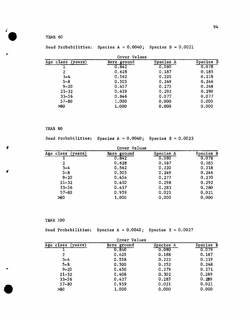
J• YEAR 60

Seed Probabilities: Species A = 0.0040; Species B = 0.0021

94

Age class (years)123-45-89-20

21-3233-5657-80

>80

Cover ValuesBare ground

0.8420.6280.5620.5050.4570.4190.8461.0001.000

Species A0.0800.1870.2200.2490.2750.2920.0770.0000.000

Species B0.0780.1850.2180.2460.2680.2900.0770.0000.000

YEAR 80

Seed Probabilities: Species A = 0.0040; Species B = 0.0023

Cover ValuesAge class (years) Bare ground Species A Species B

1 0.842 0.080 0.0782 0.628 0.187 0.1853-4 0.562 0.220 0.2185-8 0.505 0.249 0.2469-20 0.454 0.277 0.270

21-32 0.410 0.298 0.29233-56 0.437 0.283 0.28057-80 0.959 0.021 0.021

>80 1.000 0.000 0.000

YEAR 100

Seed Probabilities: Species A = 0.0040; Species B = 0.0027

•

•

Age class (years)123-45-89... 20

21-3233-5657-80

>80

Cover ValuesBare ground

0.8400.6250.5580.5000.4500.4080.4370.9591.000

Species A0.0800.1880.2220.2520.2790.3020.2830.0210.000

Species B0.0790.1870.2190.2480.2710.2890.2800.0210.000

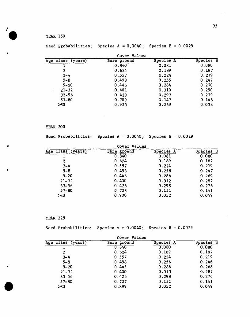
YEAR 150

Seed Probabilities: Species A = 0.0040j Species B = 0.0029

95

Age class (years)123-45-89-20

21-3233-5657-80

>80

Cover ValuesBare ground

0.8400.6240.5570.4980.4460.4010.4290.7090.923

Species A0.0810.1890.2240.2550.2840.3100.2930.1470.039

Species B0.0800.1870.2190.2470.2700.2900.2790.1430.038

YEAR 200

Seed Probabilities: Species A = 0.0040j Species B = 0.0029

Cover valuesAge class (years) Bare ground Species A Species B

1 0.840 0.081 0.0802 0.624 0.189 0.1873-4 0.557 0.224 0.2195-8 0.498 0.256 0.2479-20 0.446 0.286 0.269

21-32 0.400 0.312 0.28733-56 0.426 0.298 0.27657-80 0.708 0.151 0.141

>80 0.900 0.052 0.049

YEAR 225

Seed Probabilities: Species A = 0.0040j Species B = 0.0029

•

Age class (years)123-45-89-20

21-3233-5657-80

>80

Cover ValuesBare ground

0.8400.6240.5570.4980.4450.4000.4260.7070.899

Species A0.0800.1890.2240.2560.2860.3130.2980.1520.052

Species B0.0800.1870.2190.2460.2680.2870.2760.1410.049

FINAL TRANSITION MATRICES

TM1

96

Transition to 1/2 yearBare Species A0.845 0.0770.044 0.9280.045 0.028

age classSpecies B

0.0770.0280.927

TM2

Transition from1 year age class

BareSpecies ASpecies B

Transition to 1 yearBare Species A0.742 0.1290.002 0.9310.003 0.071

age classSpecies B

0.1290.0670.926

TM3

Transition from1 year age class

BareSpecies ASpecies B

Transition to 3-4 yearBare Species A0.893 0.0540.001 0.9620.001 0.048

Transition to 5-8 yearBare Species A0.894 0.0530.001 0.9660.001 0.044

age classSpecies B

0.0530.0380.952

age classSpecies B

0.0530.0340.955

TM4

TM5

Transition from2 year age class

BareSpecies ASpecies B

Transition from3-4 year age class

BareSpecies ASpecies B

•

Transition to 9-20 yearBare Species A0.895 0.0530.000 0.9950.001 0.023

age classSpecies B

0.0520.0050.977

Transition from5-8 year age class

BareSpecies ASpecies B

97t• TM6

Transition to 21-32 year age class Transition from

• Bare Species A Species B 9-20 year age class0.897 0.052 0.051 Bare0.001 0.993 0.006 Species A0.001 0.021 0.977 Species B

TM7

Transition to 33-56 year age class Transition fromBare Species A Species B 21-32 year age class0.924 0.038 0.038 Bare0.093 0.897 0.010 Species A0.093 0.011 0.896 Species B

TM8

Transition to 57-80 year age class Transition fromBare Species A Species B 33-56 year age class0.998 0.001 0.001 Bare..0.492 0.498 0.010 Species A0.492 0.010 0.498 Species B

~TM9

Transition to >80 year age class Transition fromBare Species A Species B 57-80 year age class0.998 0.001 0.001 Bare0.495 0.500 0.005 Species A0.495 0.005 0.500 Species B

..

-.

SIMULATION 4

YEAR 10

Seed Probabilities: Species A = 0.0010; Species B = 0.0010

98

Age class (years)123-45-89-20

21-3233-5657-80

>80

Cover ValuesBare ground

0.8480.6370.5750.7831.0001.0001.0001.0001.000

Species A0.0760.1810.2120.1090.0000.0000.0000.0000.000

Species B0.0760.1820.2130.1090.0000.0000.0000.0000.000

YEAR 20

Seed Probabilities: Species A = 0.0010; Species B = 0.0010

Cover ValuesAge class (years) Bare ground Species A Species B

1 0.847 0.076 0.076~. 2 0.636 0.182 0.182

3-4 0.573 0.213 0.2145-8 0.518 0.241 0.2429-20 0.803 0.099 0.099

21-32 1.000 0.000 0.00033-56 1.000 0.000 0.00057-80 1.000 0.000 0.000

>80 1.000 0.000 0.000

YEAR 40

Seed Probabilities: Species A = 0.0015; Species B =0.0015

Cover ValuesAge Class (years) Bare ground Species A Species B

1 0.845 0.077 0.0772 0.632 0.183 0.1843-4 0.568 0.214 0.2175-8 0.512 0.242 0.2469-20 0.467 0.266 0.267

21-32 0.811 0.094 0.094

• 33-56 1.000 0.000 0.00057-80 1.000 0.000 0.000

>80 1.000 0.000 0.000

•• YEAR 60

Seed Probabilities: Species A = 0.0021; Species B = 0.0022

99

Age class (years)123-45-89-20

21-3233-5657-80

>80

Cover ValuesBare ground

0.8430.6290.5630.5060.4580.4200.846LOOO1.000

Species A0.0780.1840.2150.2430.2700.2890.0770.0000.000

Species B0.0780.1870.2210.2510.2720.2910.0770.0000.000

YEAR 80

Seed Probabilities: Species A = 0.0023; Species B = 0.0023

Cover ValuesAge class (years) Bare ground Species A Species B

1 0.843 0.078 0.0782 0.629 0.184 0.1873-4 0.563 0.216 0.2215-8 0.506 0.243 0.2519-20 0.455 0.270 0.275

21-32 0.411 0.292 0.29633-56 0.438 0.280 0.28257...80 0.959 0.021 0.021

>80 LOOO 0.000 0.000

YEAR 100

Seed Probabilities: Species A = 0.0028; Species B = 0.0028

•

Age class (years)123-45...89-20

21..3233..5657... 80

>80

Cover ValuesBare ground

0.8410.6260.5590.5010.4510.4090.4380.9591.000

Species A0.0790.1850.2160.2430.2710.2950.2800.0210.000

Species B0.0790.1890.2250.2560.2780.2950.2820.0210.000

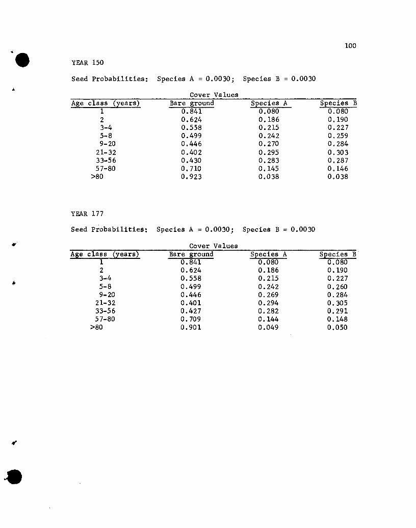
~.YEAR 150

Seed Probabilities: Species A = 0.0030j Species B = 0.0030

100

Age class (years)123-45-89-20

21-3233-5657.,.80

>80

Cover ValuesBare ground

0.8410.6240.5580.4990.4460.4020.4300.7100.923

Species A0.0800.1860.2150.2420.2700.2950.2830.1450.038

Species B0.0800.1900.2270.2590.2840.3030.2870.1460.038

YEAR 177

Seed Probabilities: Species A = 0.0030j Species B = 0.0030

.' Cover ValuesAge class (years) Bare ground Species A Species B

1 0.841 0.080 0.0802 0.624 0.186 0.1903-4 0.558 0.215 0.227

~ 5-8 0.499 0.242 0.2609-20 0.446 0.269 0.284

21-32 0.401 0.294 0.30533-56 0.427 0.282 0.29157-80 0.709 0.144 0.148

>80 0.901 0.049 0.050

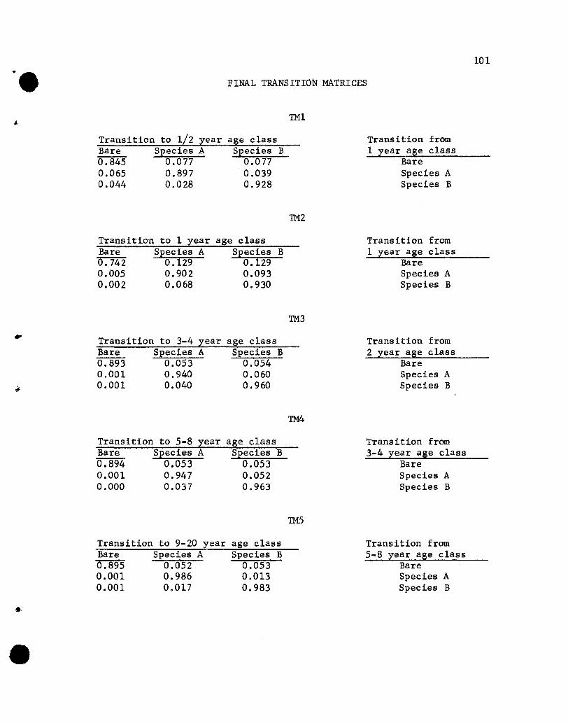
•• FINAL TRANSITION MATRICES

TM1

101

Transition to 1/2 yearBare Species A0.845 0.0770.065 0.8970.044 0.028

age classSpecies B

0.0770.0390.928

TM2

Transition from1 year age class

BareSpecies ASpecies B

Transition to 1 yearBare Species A0.742 0.1290.005 0.9020.002 0.068

age classSpecies B

0.1290.0930.930

Transition from1 year age class

BareSpecies ASpecies B

TM3

Transition to 3-4 year age classBare Species A Species B0.893 0.053 0.0540.001 0.940 0.060

~0.001 0.040 0.960

TM4

Transition to 5-8 year age classBare Species A Species B0.894 0.053 0.0530.001 0.947 0.0520.000 0.037 0.963

TM5

Transition to 9-20 year age classBare Species A Species B0.895 0.052 0.0530.001 0.986 0.0130.001 0.017 0.983

•

•

Transition from2 year age class

BareSpecies ASpecies B

Transition from3-4 year age class

BareSpecies ASpecies B

Transition from5-8 year age class

BareSpecies ASpecies B

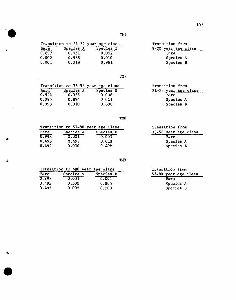
102v.TM6

Transition to 21-32 year age class Transition fromBare Species A Species B 9-20 year age class0.897 0.051 0.052 Bare0.002 0.988 0.010 Species A0.001 0.018 0.981 Species B

TM7

Transition to 33-56 year age class Transition fromBare Species A Species B 21-32 year age classO. 924 0.038 0.038 Bare0.095 0.894 0.011 Species A0.093 0.010 0.896 Species B

TM8

Transition to 57-80 year age class Transition fromBare Species A Species_B 33-56 year age class0.998 0.001 0.001 Bare..0.493 0.497 0.010 Species A0.492 0.010 0.498 Species B

~ TM9

Transition to >80 year age class Transition fromBare Species A Species B 57-80 year age class0.998 0.001 0.001 Bare0.495 0.500 0.005 Species A0.495 0.005 0.500 Species B

•

~.

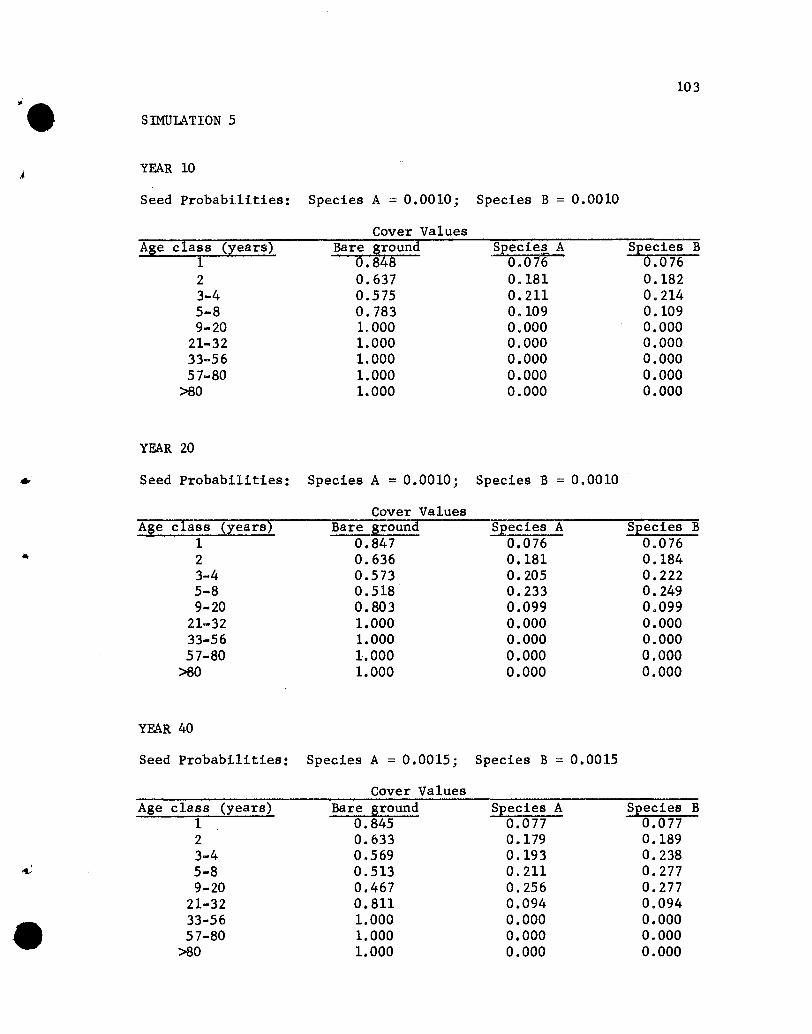
J

SIMULATION 5

YEAR 10

Seed Probabilities: Species A = 0.0010; Species B = 0.0010

103

Age class (years)123-45-89-20

21-3233-5657-80

>80

Cover ValuesBare ground

0.8480.6370.5750.7831.0001.0001.0001.0001.000

Specie!!. A0.0760.1810.2110.1090.0000.0000.0000.0000.000

Species B0.0760.1820.2140.1090.0000.0000.0000.0000.000

YEAR 20

• Seed Probabilities: Species A = 0.0010; Species B = 0.0010

Cover ValuesAge class (years) Bare ground Species A Species B

1 0.847 0.076 0.076.. 2 0.636 0.181 0.1843..4 0.573 0.205 0.2225-8 0.518 0.233 0.2499-20 0.803 0.099 0.099

21-32 1.000 0.000 0.00033-56 1.000 0.000 0.00057-SO l.000 0.000 0.000

>80 1.000 0.000 0.000

YEAR 40

Seed Probabilities: Species A = 0.0015; Species B = 0.0015

Cover ValuesAge class (years) Bare ground Species A Species B

1 0.845 0.077 0.0772 0.633 0.179 0.1893-4 0.569 0.193 0.238

~ 5-8 0.513 0.211 0.2779-20 0.467 0.256 0.277

21-32 0.811 0.094 0.094

• 33-56 1.000 0.000 0.00057-80 1.000 0.000 0.000

>80 1.000 0.000 0.000

-. YEAR 60

Seed Probabilities: Species A == 0.0020; Species B == 0.0022

104

)

Age class (years)123-45-89-20

21-3233-5657-80

>80

YEAR 80

Cover ValuesBare ground

0.8430.6290.5640.5070.4590.4200.8461.0001.000

Species A0.0780.1730.1700.1740.2130.2650.0770.0000.000

Species B0.0790.1980.2660.3200.3280.3160.0770.0000.000

Seed Probabilities: Species A == 0.0021; Species B = 0.0026

..

Age class (years)123-45-89-20

21-3233-5657-80

>80

Cover ValuesBare ground

0.8430.6290.5630.5060.4550.4110.4380.9591.000

Species A0.0780.1710.1630.1600.1750.2120.2440.0210.000

Species B0.0790.2000.2740.3340.3700.3760.3180.0210.000

YEAR 100

Seed Probabilities: Species A == 0.0022; Species B == 0.0033

Cover ValuesAge class (years) Bare ground Species A Species B

1 0.841 0.079 0.0802 0.625 0.159 0.2153-4 0.559 0.116 0.3255-8 0.500 0.099 0.401

;: 9-20 0.451 0.135 0.41421-32 0.409 0.183 0.40833-56 0.438 0.244 0.318

• 57-80 0.959 0.021 0.021>80 1.000 0.000 0.000

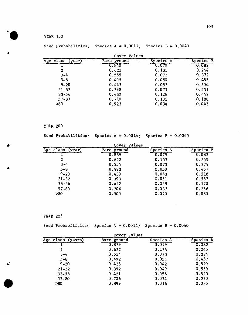
~. YEAR 150

Seed Probabilities: Species A = 0.0017; Species B = 0.0040

105

Age class (year)123-45-89-20

21-3233-5657-80

>80

Cover ValuesBare ground

0.8400.6230.5550.4950.4430.3980.4300.7100.923

Species A0.0790.1330.0730.0500.0530.0710.1280.1030.034

Species B0.0820.2440.3720.4550.5040.5310.4420.1880.043

YEAR 200

Seed Probabilities: Species A = 0.0014; Species B = 0.0040

... Cover ValuesAge class (year) Bare ground Species A Species B

1 0.839 0.079 0.0822 0.622 0.133 0.2453-4 0.554 0.073 0.374

• 5-8 0.493 0.050 0.4579-20 0.439 0.043 0.518

21-32 0.393 0.051 0.55733-56 0.422 0.059 0.52057-80 0.706 0.037 0.256

>80 0.900 0.020 0.080

YEAR 225

Seed Probabilities: Species A = 0.0014; Species B = 0.0040

•

Age class (years)123-45-89-20

21-3233-5657-80

>80

Cover ValuesBare ground

0.8390.6220.5540.4920.4380.3920.4210.7060.899

Species A0.0790.1330.0730.0510.0420.0490.0560.0340.016

Species B0.0820.2450.3740.4570.5200.5590.5230.2600.085

.i.e FINAL TRANSITION MATRICES

TMl

106

Transition to 1/2 yearBare Species A0.843 0.0780.408 0.3610.030 0.033

age classSpecies B

0.0780.2310.937

TM2

Transition from1 year age class

BareSpecies ASpecies B

Transition to 1 yearBare Species A0.738 0.1300.038 0.3000.000 0.000

age classSpecies B

0.1320.6631.000

TM3

Transition from1 year age class

BareSpecies ASpecies B

•

Transition to 3-4 yearBare Species A0.889 0.0530.006 0.2990.000 0.000

Transition to 5-8 yearBare Species A0.888 0.0520.007 0.2980.000 0.000

age classSpecies B

0.0590.6951.000

age classSpecies B

0.0600.6951.000

TM4

TM5

Transition from2 year age class

BareSpecies ASpecies B

Transition from3-4 year age class

BareSpecies ASpecies B

•

Transition to 9-20 yearBare Species A0.890 0.0520.003 0.3170.000 0.000

age classSpecies B

0.0590.6791.000

Transition from5~8 year age class

BareSpecies ASpecies B

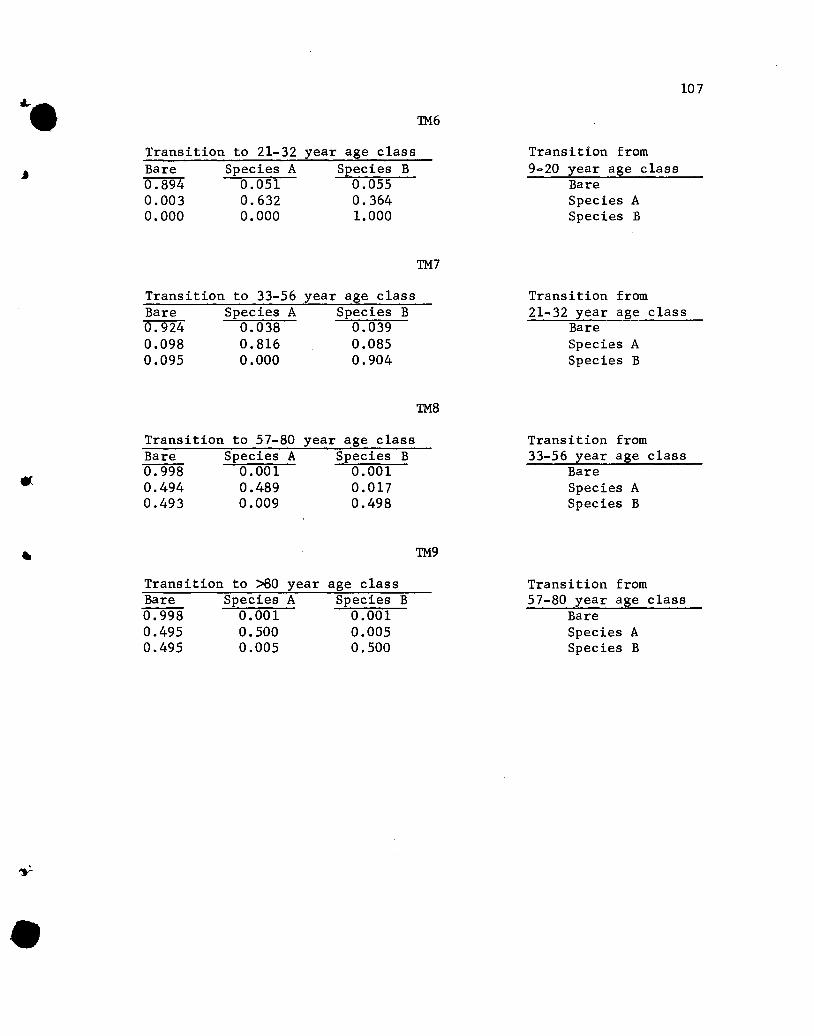
107Le 1M6

Transition to 21-32 year age class Transition fromBare Species A Species B 9-20 year age class0.894 0.051 0.055 Bare0.003 0.632 0.364 Species A0.000 0.000 1.000 Species B

TM7

Transition to 33-56 year age class Transition fromBare Species A Species B 21-32 year age class0.924 0.038 0.039 Bare0.098 0.816 0.085 Species A0.095 0.000 0.904 Species B

1M8

Transition to 57-80 year age class Transition fromBare Species A Species B 33-56 year age class

fl.0.998 0.001 0.001 Bare0.494 0.489 0.017 Species A0.493 0.009 0.498 Species B

• 1M9

Transition to >80 year age class Transition fromBare Species A Species B 57-80 year age class0.998 0.001 0.001 Bare0.495 0.500 0.005 Species A0.495 0.005 0.500 Species B

•