Business Statistics Intro to R - Booth School of...

Business StatisticsIntro to R

Contents

1 First R 3

2 Reading Data into R, Simple Summaries and Plot 5

3 Source Files, Comments, and Sink 8

4 Getting Help in R, More on Plotting 10

5 Histogram, Time Series Plot, Color Coding 11

6 Regression in R 12

7 Factors, Tables, and attach 15

8 Working with Text 17

9 Logical Variables and Subsetting Your Data 18

10 sapply and tapply 20

11 Adding Points, Lines, and Text to a Plot 21

12 Package Installation 22

1

Note:

At the end of some sections are suggested supplemental reading in the book “Introductory

Statistics with R” by Peter Dalgaard. I chose this book because it seems well written and

has relatively simple and useful discussions of R and statistics. That being said, if you read

Dalgaard, relax. If you don’t understand something, don’t worry and focus on the parts you

get. If something is bugging you, ask me or the TA. To keep things simple, I’m only going

to point you to stuff in the introductory chapters 1 and 2 of Dalgaard even thought we look

at stuff from later chapters. Feel free to look at what Dalgaard has to say about Histograms

(chapter 4) or anything else if you want and you can easily find where to look in the contents

of the book.

Appendix C of the Dalgaard book has a very hand summary of the most important functions.

Note the for assignment Dalgaard uses x← 2, whereas I use x = 2.

They are the same, it is a matter of taste.

For those of you want a more advanced treatment of R, get “An Introduction to R” from the

R website. Some of this is easy and some not. But again, read the parts you get and don’t

worry about getting everything in it.

2

1 First R

First, install R.

• Go to http://www.r-project.org/.

• On the left, click on CRAN, under Download, Packages.

• choose a mirror (I guess something geographically close).

• Click on Download R for Windows (or for MacOSX,Linux).

• click on base.

• click on Download R x.x.x for Windows.

Note: http://www.r-project.org/ will take you to the main R page.

To go directly to the R download page you can use http://www.cran.r-project.org/.

After than it should be pretty standard.

You will have an R icon on your desktop and all you have to do is (double) click on that.

Get into R.

At the prompt (>) type x=2 (then hit return):

> x=2

Then,

> x

Now try,

> y=3

> z=x+y

> z

> w=sqrt(x)

> w

> ls()

> rm(x)

> ls()

Things like x above are variables. We can store information in variables and then operate

on them (e.g. add them).

3

Something like sqrt is a function. Above, the function sqrt takes the argument x and

returns the square root of the value in x which we put into w.

ls is also a function, but we give it no arguments. We do not keep what it returns, so the

results are just printed to the screen. ls shows us all the variables we have created. What

does rm do?

Try:

> x=2

> x*x

[1] 4

> x^2

[1] 4

> log(x)

[1] 0.6931472

Note you can nest (or compose) functions:

> x=2

> y=3

> w = log(sqrt(x+y^2))

Try:

> x=c(5,3,7)

> x

[1] 5 3 7

> x[1]

[1] 5

> x[3]

[1] 7

> x[1:2]

[1] 5 3

> mean(x)

[1] 5

4

Here the variable x is a vector of numbers instead of just one number as is the case with x=2.

In R, variables can be numbers, strings, vectors, matrices and all kinds of very useful things!

Arithmetic works with vectors:

> x=c(1,2,3)

> y=c(4,5,6)

> w=x+y

> w

[1] 5 7 9

> z = 2*x+y

> z

[1] 6 9 12

> v=log(x)

> v

[1] 0.0000000 0.6931472 1.0986123

To get out of R use the q function:

> q()

Note that q is a function with no arguments here and you need the ()!

See also Dalgaard: Appendix A, 1.1.1-1.1.3.

2 Reading Data into R, Simple Summaries and Plot

Let’s get some data into R so we can do some statistics.

First pick a directory on your machine where you want to work. Next get the data file

“housedata.txt” from the webpage and put it in your working directory.

housedata.txt is a simple ascii file. Use a texteditor (e.g. WordPad) to look at it.

Now go into R.

The first thing you have to do is tell R what directory you want to work in.

5

To find out the current R working directory use

> getwd()

To change the working directory to be the one you put the data in use

> setwd(dname)

where dname is the working directory.

For example, on my machine I used

> setwd("C:/Users/rem/Rplay")

In Windows you can also use the menu item /File/Change dir.

To make sure you are now in the directory you put the data in use menu /File/Display file(s)

in Windows and

> system("ls")

on the Mac.

You should see the file housedata.txt there.

To read the data in, we use the function read.table.

> hd = read.table("housedata.txt",header=TRUE)

The function will read in the data and store it in the variable hd. Of course, you can use

any name you want instead of hd. Some people like long variable names and some people

like short ones.

Here the function read.table uses two arguments. The first one, "housedata.txt" tells it

what file to read the data from, while the second header=TRUE, tells it to interpret the first

row of the file as variable names.

Be careful in Windows!!!! Windows has this nasty habit of displaying a file with name

housedata.txt as just housedata.

To print out the data set in R we can just use

> hd

The variable hd is clearly much more complicated than the variable x in x=2. x is just a

number, while hd is a value of type data.frame. A value of type data.frame has all the

6

numbers plus basic info about the data set.

Try:

> dim(hd)

> names(hd)

> ncol(hd)

> nrow(hd)

Of course, if you used a different name than hd for the data set, you would use that name

instead.

The columns of a data.frame are the variables in our data set and the rows are the obser-

vations. You can pick off columns, rows, and values from the data.frame.

Try:

> hd[,1]

> hd$Size

> mean(hd$Size)

> hd[1,]

> hd[1,2]

> sd(hd$Price)

> cor(hd$Size,hd$Price)

> hd[1:5,]

Try:

> summary(hd)

This summarizes the values in each column (or variable) of the data.frame hd.

Try:

> plot(hd[,1],hd[,2])

> plot(hd$Size,hd$Price)

> plot(hd)

To save the plot the a file in pdf format use

> dev.copy2pdf(file="houseplot.pdf",height=10,width=10)

7

where you are free to choose the file name (instead of houseplot.pdf) and the height and

width.

See also Dalgaard: 1.1.5,1.2.10,1.2.11,1.2.13.

3 Source Files, Comments, and Sink

Obviously, it can get very tiresome typing in commands!!

What you do is put all the commands you want to use into a text file and then you can edit

the file.

So, for example, if we wanted to plot the house data we could create a file with the following

lines:

hd = read.table("housedata.txt",header=TRUE)

print("Just read in house data with variables")

print(names(hd))

print("and dimensions")

print(dim(hd))

plot(hd)

dev.copy2pdf(file="hplot.pdf",height=8,width=8)

Note that at the prompt > we can just type a variable name to print it out. In files of

commands it is safer to explicitly use the print function.

Then, there are two ways to proceed.

The easiest thing to do is to simply cut and paste the commands into the intepreter window.

Try this.

The other thing to do is to “source” the file.

Suppose the file with commands is called “comR.txt” and it is in the working directory.

Then you can enter

> source("comR.txt")

and it will execute the commands in the file line by line.

I guess most people cut and paste. I tend to use source.

8

The files with commands can get complicated when the analysis does. It is important to add

comments to that you know what is going on. On any line, everything after # is ignored.

So the file might look like:

#file to read in and plot the house price data


# write out names and dim

print(names(hd))

print(dim(hd))

plot(hd) #this will do the plot

#write plot to file


If your are using Windows, check out the menu

File/New Script.

What is you want to save some stuff? Try:

sink("temp.txt")

cat("The numbers from one to ten:\n") # \n is a carriage return

print(1:10)

sink()

After the first sink all output will go to the file temp.txt rather than the screen. Remember

to use sink() to redirect output to the screen.

You can get a simple text editor to modify and look at a data frame.

Try:

> hd2 = edit(hd)

This will create a new data-frame hd2 and leave hd alone.

See also Dalgaard: 2.1.2, 2.1.3

9

4 Getting Help in R, More on Plotting

To plot the house price data we can just “run” the file:

#file to read in and plot the house price data


# write out names and dim

print(names(hd))

print(dim(hd))

plot(hd) #this will do the plot

#write to file


However, we might want to change the scale of the plot or the color or lots of other things.

To find out more about the plot function we can go to the R help.

> ?plot

or

> help(plot)

There a lots of great things about R. Perhaps, the help is not one of them.

Don’t worry, we will learn what we need to know as we go along.

For now, note that in the help for plot we see “’main’ an overall title for the plot”.

If we wanted a title for the plot this would lead us to try

> plot(hd,main="plot of house data")

Note that hd is a required argument, you have to tell plot what to plot. But many of the

other arguments are optional. You don’t have to tell plot what the main title should be. To

use an optional argument you use the from argname = argval, where in this case argname

is main and argval is the string “plot of house data”. For optional arguments, the software

will use a “default” value if you don’t supply one. You may, or may not, like the default.

Try the following:

> plot(hd[,1],hd[,2],xlab="house size", ylab="house price")

> plot(hd[,1],hd[,2],xlab="house size", ylab="house price",col="red")

10

> plot(hd[,1],hd[,2],xlab="house size", ylab="house price",col="red",cex=1.5)

> plot(hd[,1],hd[,2],xlab="house size", ylab="house price",col="red",cex=1.5,pch=2)

> plot(hd[,1],hd[,2],xlab="house size", ylab="house price",xlim=c(0,4))

Try

> help.start()

to get an html help window.

Click on packages and then base.

Search for “mean” in the webpage to find the help on the function.

Another useful command to get help is help.search.

Suppose we wonder how to compute a standard deviation in R.

Try

> help.search("standard deviation")

You can also use “??”, that is > ??mean

would search for help on functions related to “mean”.

A lot of people use R so it is very googleable.

Anytime you need to know anything (in R) try google.

See also Dalgaard: 2.1.4.

5 Histogram, Time Series Plot, Color Coding

Let’s look at the midcity house data set. It has more observations and more variables.

mc = read.table(’midcity.txt’,header=T)

Try

> hist(mc$Price)

When you read in the data, Price is in dollars and size is in square feet.

To change the units to thousands of dollars and thousands of square feet we can use

11

> mc$Price = mc$Price/1000

> mc$SqFt = mc$SqFt/1000

Now let’s do a histogram.

> hist(mc$Price)

Also try,

> hist(mc$Price,nclass=15,main="",xlab="Price")

Even though it is not a time series, let’s do a time series plot of the prices. That is, we just

plot them in the order they are in the file.

> plot(mc$Price,type="b",col="blue",lty=2)

Type = ”b” will cause both lines and points to be plotted.

col=”blue” is obvious.

lty=2 will cause the line to be dashed rather than solid, try some other values.

What does this one do?

> plot(mc$SqFt,mc$Price,col=mc$Nbhd,pch=16)

6 Regression in R

Let’s run a regression using the simple housing data.

#read in data


cat("dim of house data: ",dim(hd),’\n’) #this will print the dim out

#run the regression

hreg = lm(Price~Size,hd)

12

lm is the R function which performs the regression computations and then returns of lot of

information. We have stored the information in the variable hreg.

What type of variable is hreg? It is a list. A list has a bunch of named components, where

each component can be something different.

I can find out the components of the list hreg by entering

> names(hreg)

which generates

[1] "coefficients" "residuals" "effects" "rank"

[5] "fitted.values" "assign" "qr" "df.residual"

[9] "xlevels" "call" "terms" "model"

We will learn about some of these components, but some are quite advanced.

To start with, the most basic part of the result in hreg is coefficients. This give the

least-squares intercept and slope.

print(hreg$coefficients)

Which generates the output:

(Intercept) Size

38.88468 35.38596

When you “run a regression” in most statistical packages you simply get a summary output.

You can get this in R by doing

print(summary(hreg))

which generates the output:

13

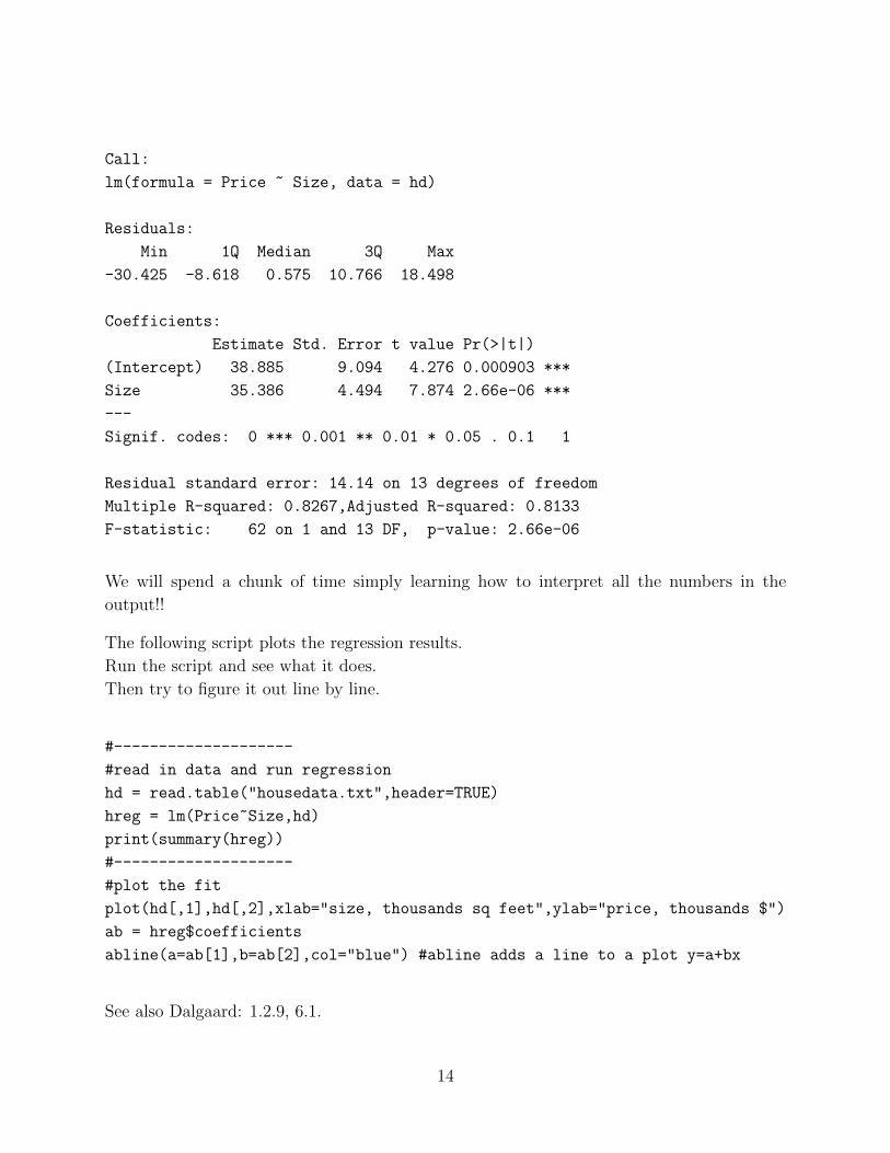
Call:

lm(formula = Price ~ Size, data = hd)

Residuals:

Min 1Q Median 3Q Max

-30.425 -8.618 0.575 10.766 18.498

Coefficients:

Estimate Std. Error t value Pr(>|t|)

(Intercept) 38.885 9.094 4.276 0.000903 ***

Size 35.386 4.494 7.874 2.66e-06 ***

---

Signif. codes: 0 *** 0.001 ** 0.01 * 0.05 . 0.1 1

Residual standard error: 14.14 on 13 degrees of freedom

Multiple R-squared: 0.8267,Adjusted R-squared: 0.8133

F-statistic: 62 on 1 and 13 DF, p-value: 2.66e-06

We will spend a chunk of time simply learning how to interpret all the numbers in the

output!!

The following script plots the regression results.

Run the script and see what it does.

Then try to figure it out line by line.

#--------------------

#read in data and run regression


hreg = lm(Price~Size,hd)

print(summary(hreg))

#--------------------

#plot the fit

plot(hd[,1],hd[,2],xlab="size, thousands sq feet",ylab="price, thousands $")

ab = hreg$coefficients

abline(a=ab[1],b=ab[2],col="blue") #abline adds a line to a plot y=a+bx

See also Dalgaard: 1.2.9, 6.1.

14

7 Factors, Tables, and attach

Let’s get the midcity housing data and have a look at it.

mc = read.table("midcity.txt",header=T)

mc=mc[,c(2,4,5,6,8)]

mc$Price = mc$Price/1000

mc$SqFt = mc$SqFt/1000

print(summary(mc))

print(mc[1:5,])

Notice that R summarizes the Brick variable differently.

R sees that the variable must be categorical and gives the counts for each category.

However, R has no way of knowing that Nbhd is categorical and reports the mean (which

does not make sense).

R has the ability to label each variable in a data-frame as being categorical or numeric.

Then it will treat the variable differently according to its structure.

R uses the term factor for a categorical variable.

Try

> is.factor(mc$Brick)

> is.factor(mc$Price)

> is.factor(mc$Nbhd)

> is.numeric(mc$Nbhd)

We need R to understand that Nbhd is a factor/categorical variable.

To change Nbhd to a factor:

> mc$Nbhd = as.factor(mc$Nbhd)

Now try,

> is.factor(mc$Nbhd)

and

> summary(mc)

15

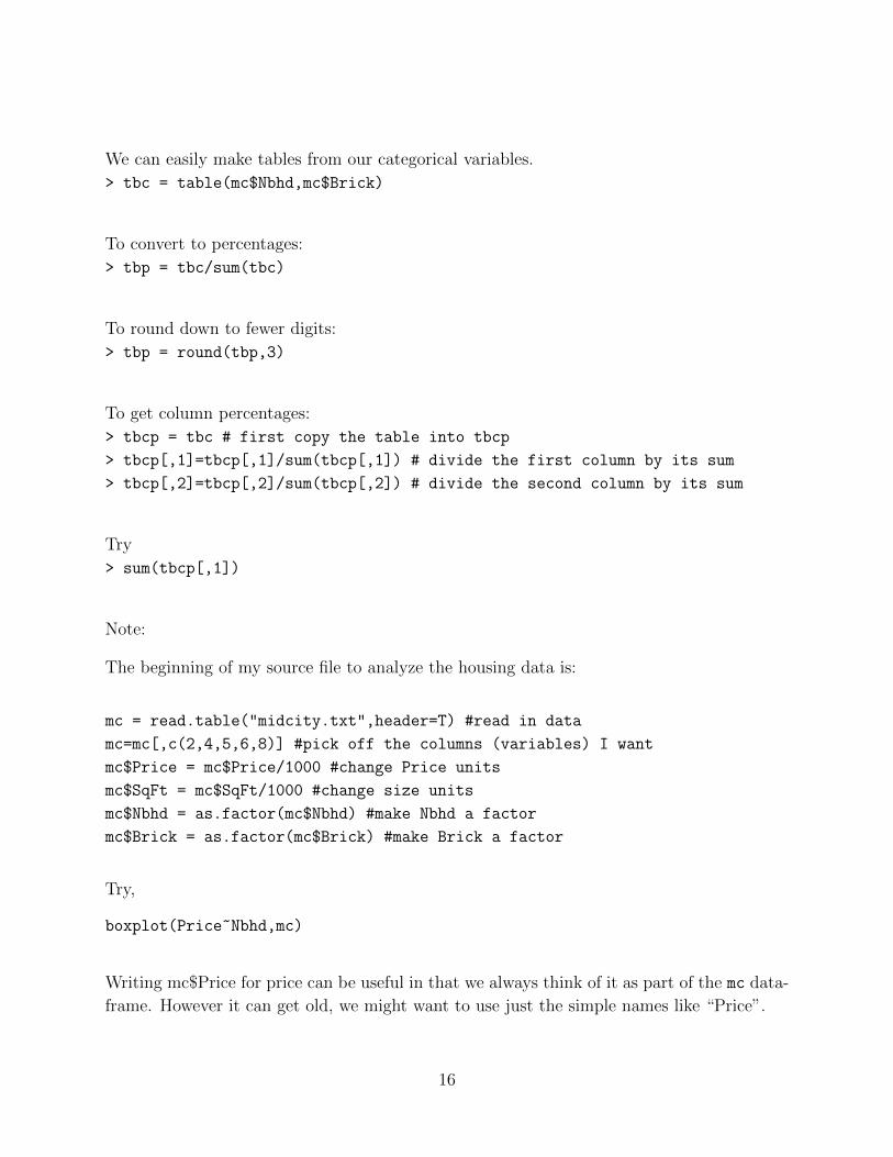
We can easily make tables from our categorical variables.

> tbc = table(mc$Nbhd,mc$Brick)

To convert to percentages:

> tbp = tbc/sum(tbc)

To round down to fewer digits:

> tbp = round(tbp,3)

To get column percentages:

> tbcp = tbc # first copy the table into tbcp

> tbcp[,1]=tbcp[,1]/sum(tbcp[,1]) # divide the first column by its sum

> tbcp[,2]=tbcp[,2]/sum(tbcp[,2]) # divide the second column by its sum

Try

> sum(tbcp[,1])

Note:

The beginning of my source file to analyze the housing data is:

mc = read.table("midcity.txt",header=T) #read in data

mc=mc[,c(2,4,5,6,8)] #pick off the columns (variables) I want

mc$Price = mc$Price/1000 #change Price units

mc$SqFt = mc$SqFt/1000 #change size units

mc$Nbhd = as.factor(mc$Nbhd) #make Nbhd a factor

mc$Brick = as.factor(mc$Brick) #make Brick a factor

Try,

boxplot(Price~Nbhd,mc)

Writing mc$Price for price can be useful in that we always think of it as part of the mc data-

frame. However it can get old, we might want to use just the simple names like “Price”.

16

Try,

> attach(mc)

> plot(SqFt,Price)


8 Working with Text

Text is very useful for labeling plots and naming variables and other stuff.

Our variables can be text:

> x = "R is great"

> x

We can also have vectors of text:

> tv = c("R","is","great")

> tv[1]

This is very useful for naming the variables in a data frame.

Suppose we have read in the midcity housing data and called the data-frame mc as above.

> names(mc)

If we would like to change the name SqFt to Size we could use:

> names(mc)[2] = "Size"

> names(mc)

We could change all the names at one time

> names(mc) = c("NBHD","SIZE","BRICK","BEDS","PRICE")

> names(mc)

Another kind of name you might want to change is the name assigned to a category for a

factor.

17

Try:

> attach(mc)

> table(NBHD,BRICK)

R calls the categories “levels”.

> levels(NBHD) = c("N1","N2","N3")

> table(NBHD,BRICK)

A very useful function for working with text is paste.

Try:

> paste("R","is","great")

> paste("R","is","great",sep="a")

> paste("R","is","great",sep="")

> levels(NBHD) = paste("NBHD",1:3,sep="")

> table(NBHD)

> plot(SIZE,PRICE,main=paste("correlation is ",cor(SIZE,PRICE),sep=""))

> plot(SIZE,PRICE,main=paste("correlation is ",round(cor(SIZE,PRICE),3),sep=""))


9 Logical Variables and Subsetting Your Data

Another kind of variable which is very useful a logical variable.

> 1>2

> 2>1

> 2==1

> 2==2

> 2=>2

18

There are only two possible values, TRUE or FALSE.

What is really useful are vectors of logical values.

> x=1:10

> x<6

We can use this to pick off interesting subsets of our data.

> x=1:10

> y=sample(1:10)# randomly permute 1 to 10

> xx = x[y>5]

> xx

Or,

> x=1:10

> y=sample(1:10)# randomly permute 1 to 10

> yg5 = y>5

> yg5

> xx = x[yg5]

> xx

Well, that is not interesting, but how about:

par(mfrow=c(1,3)) #set up three plots in a 1 x 3 arrangement

attach(mc)

hist(Price[Nbhd=="1"],xlim=c(67,215))



See also Dalgaard: 1.2.3,1.2.12

19

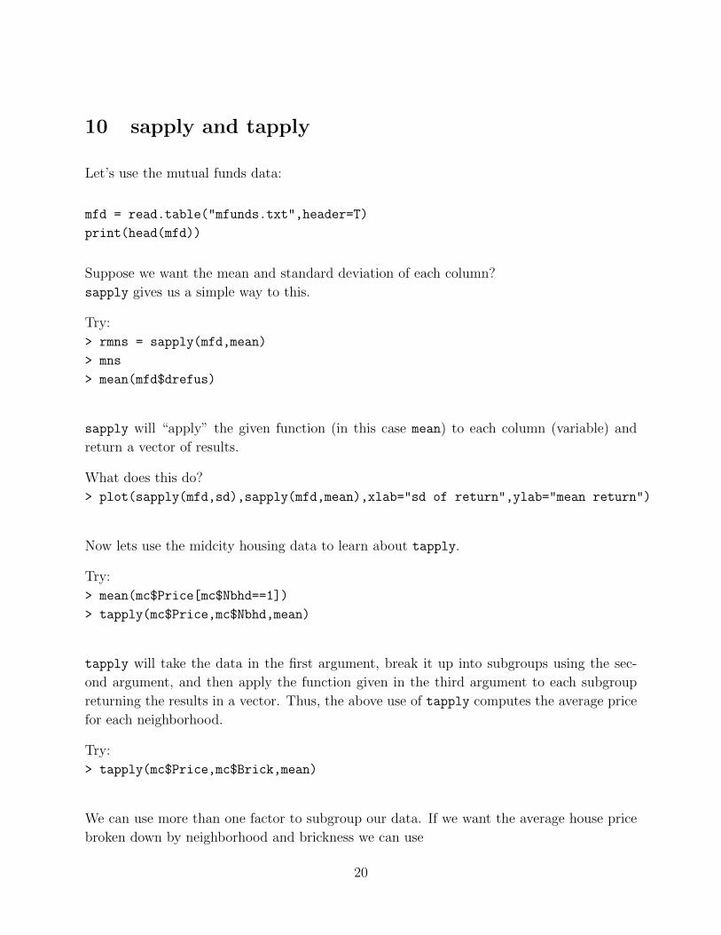
10 sapply and tapply

Let’s use the mutual funds data:

mfd = read.table("mfunds.txt",header=T)

print(head(mfd))

Suppose we want the mean and standard deviation of each column?

sapply gives us a simple way to this.

Try:

> rmns = sapply(mfd,mean)

> mns

> mean(mfd$drefus)

sapply will “apply” the given function (in this case mean) to each column (variable) and

return a vector of results.

What does this do?

> plot(sapply(mfd,sd),sapply(mfd,mean),xlab="sd of return",ylab="mean return")

Now lets use the midcity housing data to learn about tapply.

Try:

> mean(mc$Price[mc$Nbhd==1])

> tapply(mc$Price,mc$Nbhd,mean)

tapply will take the data in the first argument, break it up into subgroups using the sec-

ond argument, and then apply the function given in the third argument to each subgroup

returning the results in a vector. Thus, the above use of tapply computes the average price

for each neighborhood.

Try:

> tapply(mc$Price,mc$Brick,mean)

We can use more than one factor to subgroup our data. If we want the average house price

broken down by neighborhood and brickness we can use

20

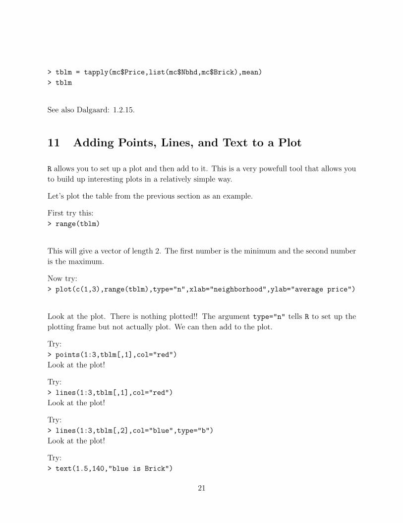
> tblm = tapply(mc$Price,list(mc$Nbhd,mc$Brick),mean)

> tblm


11 Adding Points, Lines, and Text to a Plot

R allows you to set up a plot and then add to it. This is a very powefull tool that allows you

to build up interesting plots in a relatively simple way.

Let’s plot the table from the previous section as an example.

First try this:

> range(tblm)

This will give a vector of length 2. The first number is the minimum and the second number

is the maximum.

Now try:

> plot(c(1,3),range(tblm),type="n",xlab="neighborhood",ylab="average price")

Look at the plot. There is nothing plotted!! The argument type="n" tells R to set up the

plotting frame but not actually plot. We can then add to the plot.

Try:

> points(1:3,tblm[,1],col="red")

Look at the plot!

Try:

> lines(1:3,tblm[,1],col="red")

Look at the plot!

Try:

> lines(1:3,tblm[,2],col="blue",type="b")

Look at the plot!

Try:

> text(1.5,140,"blue is Brick")

21

> text(2.5,120,"red is non-Brick",col="red")

What does this do?

mfd = read.table(paste(ddir,’mfunds.txt’,sep=’’),header=T)

plot(sapply(mfd,sd),sapply(mfd,mean),type="n",xlab="stan dev",ylab="mean")

text(sapply(mfd,sd),sapply(mfd,mean),names(mfd))

12 Package Installation

A key advantage to R is the many “packages” that have been written for R.

These are add-ons the the base system that give you additional functionality.

Often the latest research is available in these packages and, of course, the price is zero.

Installing a package is very easy.

To install a package, you just need to know its name.

For example, the name of the package providing data sets for the Dalgaard book is ISwR.

To install it:

> install.packages("ISwR")

After a package is installed you have to load it into your session everytime you use it. For

the ISwR package try,

> library("ISwR")

> attach(kfm)

> mean(mat.weigth)

Go to http://www.cran.r-project.org/, then click on “packages” (on the left), then click on

“Table of available packages, sorted by date of publication ”.

Wow!!!!

See also Dalgaard: Appendix A, 2.1.5.

22

Business Statistics Intro to R - Booth School of...

Documents

Transcript of Business Statistics Intro to R - Booth School of...