1

Business Cycle Theory II

(Nominal/Demand Shocks)

Introduction

Theoretical research on business cycles has branched out considerably over the last 20 years. In addition

to the Real Business Cycle branch, there is now a second major branch known as New Keynesian models.

Together, these branches go under the heading of Dynamics Stochastic General Equilibrium (DSGE)

Models.

As suggested by its name, the New Keynesian models adhere to the view held dear by old Keynesian

economists that frictions, especially in the form of price stickiness, are essential to understanding the

economy. As we will show, these models are very similar to the Keynesian IS-LM model you probably

studied in your intermediate class. The new models typically include an IS curve and a Phillips curve,

both centerpieces of the old Keynesian model. Some of the New Keynesian models also include an LM

curve, but this depends on how monetary policy is modeled.

Where new and old Keynesians differ is that New Keynesian models are founded on microeconomics,

starting at the level of preferences and technology. In this respect, the New Keynesian paradigm is more

similar to the RBC one. There is in fact a good deal of agreement between those economists who

consider themselves as practitioners of the RBC paradigm and those who consider themselves

practitioners of the New Keynesian paradigm. Practitioners of RBC theory are not adverse to the notion

that frictions are important for understanding the business cycle. Indeed, an approach known as Business

Cycle Accounting pioneered by V.V. Chari, Patrick J. Kehoe, and Ellen McGrattan provides strong

evidence that two wedges, a TFP wedge and a labor wedge, which arise because of frictions, are the

source of most of the business cycle fluctuations.

2

There are however some major differences. The first is more of a philosophical one that involves the

right amount of model abstraction. For the most part, proponents of RBC prefer simpler structures, with a

small number of model parameters. Proponents of the RBC approach are not embarrassed that their

models do not match all dimensions of the macro data. In contrast, proponents of the New Keynesian

approach prefer models that fit many more dimensions of the aggregate data. This requires the addition

of large number of features and shocks be added to the model, and with them, a large set of parameters

that need to be estimated.

An important issue, particularly with respect to the quantitative analysis used in these chapters, is whether

the New Keynesian models are being calibrated? In most cases, the assignment of parameters is done so

that the model matches or fits the data. On the face of it, this would not seem inconsistent with the

calibration procedure. However, as a pure calibration exercise a number of criticisms have been made.

Robert E. Lucas once said “Beware of Economists bearing free parameters”, and so there is a lot to be

aware of in the case of these New Keynesian models. By setting the parameters to match observations,

particularly the ones the theory is interested in accounting for, these models are not being tested as in step

5 of our calibration procedure. Many practitioners of the RBC school have criticized New Keynesians for

not using micro level data to restrict the values of these added parameters. Paul Romer from New York

University goes further in his article the Trouble with Macroeconomics to criticize the standard

approaches used by practitioners of these models to get around the identification problem associated with

the large number of parameters. He is not kind in his assessment, arguing that for the most parts

parameter values are tied down by feeding in a fact with an unknown truth value (FWUTV). Although

Dr. Romer is harsh in his criticism of the New Keynesian models, he is no fan of the RBC models either.

Despite these criticisms, there is really no other game in town for the purpose of evaluating monetary

policy. RBC models, at least the earliest versions, had nothing to say about policy. Absent frictions, the

competitive equilibrium is efficient, and there is no reason for government intervention. New Keynesian

models have become the backbone of policy analysis at most of the central banks.

3

II. Background: The Real Effects of Monetary Policy?

Sargent and Wallace (1975) showed that introducing rational expectations into the Keyneisan IS/LM

model had important implications for monetary policy. In particular, they showed that the monetary

authority could not on average change the level of the economy’s output or employment when people

formed expectations rationally. If peoples’ expectations are rational, then they cannot be making errors in

their forecasts in a systematic manner. The entire premise underlying the mechanism by which monetary

policy has real effects works through surprising firms and households. Without surprises, and assuming

some firms or workers are not locked into set prices in the period, the changes in the money supply would

have no real effect. This is the famous Neutrality of Money result, which goes back to Classical

Economics.

The neutrality of money result has come to be associated with Real Business Cycle Theory. This is a bit

unfortunate. It is little known that the working paper of Kydland and Prescott’s 1982 Econometrica

article included a monetary side. However, they found the effects of monetary shocks in the calibration

exercise to be small and so Kydland and Prescott simplified the model in the final version of the paper by

eliminating the monetary side.

Recall from our chapter on Business Cycle Facts, that M2 is procyclical with a lead of 3 to 6 months.

This would suggest that money has real effects. However, some economists argue that the positive

correlation reflects reverse causation. Reverse causation works as follows. People and firms expect a

high TFP 3 or 6 months from now. With a higher expected TFP, capital will be more productive, so

businesses will want to increase their investments and hence their demand for loans. Banks will meet

these higher loans from their excess reserves. As you probably learned in your studies of Money and

Banking, the money multiplier depends on the amount of excess reserves that the banking sector holds,

4

with the multiplier being larger when less reserves are held. This expectation of a future productivity

shock, therefore, causes the money supply to increase today.

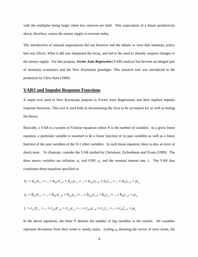
The introduction of rational expectations did not however end the debate or view that monetary policy

had real effects. What it did was sharpened the focus, and led to the need to identify surprise changes to

the money supply. For this purpose, Vector Auto Regression (VAR) analysis has become an integral part

of monetary economics and the New Keynesian paradigm. This research tool was introduced to the

profession by Chris Sims (1980).

VARS and Impulse Response Functions

A major tool used in New Keynesian analysis is Vector Auto Regressions and their implied impulse

response functions. This tool is used both in documenting the facts to be accounted for as well as testing

the theory.

Basically, a VAR is a system of N-linear equations where N is the number of variables. In a given linear

equation, a particular variable is assumed to be a linear function of its past variables as well as a linear

function of the past variables of the N-1 other variables. In each linear equation, there is also an error or

shock term. To illustrate, consider the VAR studied by Christiano, Eichenbaum and Evans (1999). The

three macro variables are inflation, πt, real GNP, yt, and the nominal interest rate, it. The VAR thus

constitutes three equations specified as

tPtiPtiPtyPtyPtPtt iaiayayaaa ......... 111111

tyPtiPtiPtyPtyPtPtt ibibybybbby ......... 111111

tiPtiPtiPtyPtyPtPtt icicycyccci ......... 111111

In the above equations, the letter P denotes the number of lag variables in the system. All variables

represent deviations from their trend or steady states. Letting μt denoting the vector of error terms, the

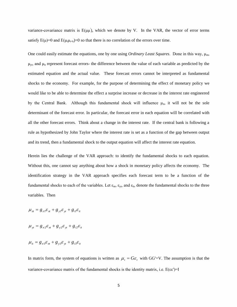
5

variance-covariance matrix is E(μμ′), which we denote by V. In the VAR, the vector of error terms

satisfy E(μ)=0 and E(μtμt+k)=0 so that there is no correlation of the errors over time.

One could easily estimate the equations, one by one using Ordinary Least Squares. Done in this way, μπt,

μyt, and μit represent forecast errors- the difference between the value of each variable as predicted by the

estimated equation and the actual value. These forecast errors cannot be interpreted as fundamental

shocks to the economy. For example, for the purpose of determining the effect of monetary policy we

would like to be able to determine the effect a surprise increase or decrease in the interest rate engineered

by the Central Bank. Although this fundamental shock will influence μit, it will not be the sole

determinant of the forecast error. In particular, the forecast error in each equation will be correlated with

all the other forecast errors. Think about a change in the interest rate. If the central bank is following a

rule as hypothesized by John Taylor where the interest rate is set as a function of the gap between output

and its trend, then a fundamental shock to the output equation will affect the interest rate equation.

Herein lies the challenge of the VAR approach: to identify the fundamental shocks to each equation.

Without this, one cannot say anything about how a shock in monetary policy affects the economy. The

identification strategy in the VAR approach specifies each forecast term to be a function of the

fundamental shocks to each of the variables. Let επt, εyt, and εit, denote the fundamental shocks to the three

variables. Then

itiytytt ggg 111

itiytytyt ggg 222

itiytytit ggg 333

In matrix form, the system of equations is written as tt G with GG′=V. The assumption is that the

variance-covariance matrix of the fundamental shocks is the identity matrix, i.e. E(εε′)=I

6

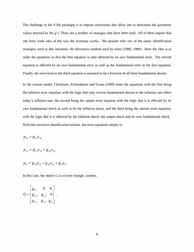
The challenge in the VAR paradigm is to impose restrictions that allow one to determine the parameter

values denoted by the g’s. There are a number of strategies that have been used. All of them require that

one have some idea of the way the economy works. We present only one of the many identification

strategies used in this literature: the Recursive method used by Sims (1980, 1989). Here the idea is to

order the equations so that the first equation is only affected by its own fundamental error. The second

equation is affected by its own fundamental error as well as the fundamental error in the first equation.

Finally, the error term in the third equation is assumed to be a function of all three fundamental shocks.

In the current model, Christiano, Eichenbaum and Evans (1999) order the equations with the first being

the inflation error equation, with the logic that only current fundamental shocks to the inflation rate affect

today’s inflation rate, the second being the output error equation with the logic that it is affected by its

own fundamental shock as well as by the inflation shock, and the third being the interest error equation,

with the logic that it is affected by the inflation shock, the output shock and its own fundamental shock .

With this recursive identification scheme, the error equations simply to

tt g 1

ytytyt gg 22

itiytytit ggg 333

In this case, the matrix G is a lower triangle, namely,

333

22

1

0

00

iy

y

ggg

gg

g

G

.

7

The matrix G is invertible and hence we can solve for the fundamental shocks as a function of the error

terms. Since we have the variance co-variance matrix of the error terms from the original system, we can

solve the matrix G since GG′=V. In this way, the VAR identifies the fundamental shocks.

After identifying the fundamental shocks, one can determine the impulse response functions of each

variable associated with any of the three fundamental shocks. The impulse response functions trace out

the values of the y, π, and i following a one unit change in one of the fundamental shocks. There are no

other shocks introduced to the system other than this shock today. For instance, we could consider how

the system is affected by a shock to interest rates. Given that we have all the parameters of the model

(i.e., a,b, c coefficients and G matrix), we can trace out the time series for inflation, output and interest

rates following a fundamental shock in the interest rate.

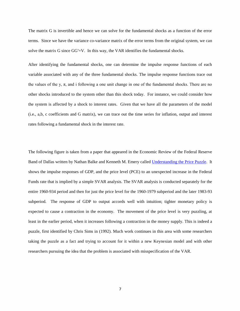
The following figure is taken from a paper that appeared in the Economic Review of the Federal Reserve

Band of Dallas written by Nathan Balke and Kenneth M. Emery called Understanding the Price Puzzle. It

shows the impulse responses of GDP, and the price level (PCE) to an unexpected increase in the Federal

Funds rate that is implied by a simple SVAR analysis. The SVAR analysis is conducted separately for the

entire 1960-934 period and then for just the price level for the 1960-1979 subperiod and the later 1983-93

subperiod. The response of GDP to output accords well with intuition; tighter monetary policy is

expected to cause a contraction in the economy. The movement of the price level is very puzzling, at

least in the earlier period, when it increases following a contraction in the money supply. This is indeed a

puzzle, first identified by Chris Sims in (1992). Much work continues in this area with some researchers

taking the puzzle as a fact and trying to account for it within a new Keynesian model and with other

researchers pursuing the idea that the problem is associated with misspecification of the VAR.

8

The impulse response functions are used both as a way of documenting the properties of business cycles

and as a way of testing the DSGE model, (typically of the New Keynesian variety). As we shall explain

more fully below, the equations of the New Keynesian model include fundamental shocks. With the

parameters of the equation in hand, one can trace out the economy’s path associated with a one-time

shock to a key component of the system.

Criticisms of VARs

VAR’s are rather controversial. They are not truly a-theoretical, nor truly theoretical. For example, in the

identification scheme used above, they require an ordering that is motivated by theory. Although

9

advances in VAR analysis now allow for a large set of variables, there is the issue of what variables

should be included. With all these questions, a valid concern is whether the impulse responses are facts,

or just artifacts of an imperfect analytical tool. For example, in the above figures, one observes that the

price level responds in a counterintuitive way. Theory suggests that an increase in the interest rate should

cause the price level to fall as the economy contracts. This counterintuitive finding is called the Price

Puzzle, being first identified by Sims (1990).

Variance Decomposition

Although, impulse response functions allow one to trace out the effect of some fundamental shock on the

endogenous variables of interest, they do not tell one how big one shocks contribution is to the overall

forecast errors. Variance Decomposition, in contrast, does just this. For the variance of each forecast

error, the contribution of each of the fundamental shocks is determined. The general finding is that the

fundamental shock to monetary policy accounts for less than 25% of the forecasting error of real gdp.

The biggest contributor to the overall variance of the forecast error of real GDP is the fundamental shock

to real GDP, εyt.

Basic New Keynesian Model

The simplest NK model consists of three equations: an IS equation, a Phillips Curve Equation and a

monetary policy rule equation.1

The IS equation

1 The model described in these pages is based on Benigno (2009)

10

The IS equation is derived using 3 equilibrium conditions. They are the utility optimizing condition that

the marginal rate of substitution between date t and t+1 consumption is equal to the gross real interest

rate, (known as the Euler Equation), the Fisher Relation, and the goods market clearing condition.

Utility Optimization

The household in each period derives utility from consumption of a final good and leisure. The

discounted stream of utility is

(PV-Utility)

0

)]()([t

tt

t NVCU

The functional form for U(Ct)

1

1)(

1

tt

CCU

And the functional form for V(Nt) is

1)(

1

tt

NNV

The inverse of the parameter, σ, is the intertemporal elasticity of substitution with respect to consumption,

and the inverse of the parameter, η, is the intertemporal elasticity of substitution with respect to labor.

These parameters determine how willing the household is willing to substitute todays consumption for

tomorrow’s consumption. Importantly, notice that utility is defined over labor. This explains the

negative sign before V(Nt).

The consumption utility optimizing condition is

(MRSC) t

t

t rC

C

11

11

In the context of business cycles, the idea is to think of period t as the short-run and period t+1 as the

long-run, or the steady state. In view of this interpretation, we will drop the time subscripts and use C to

denote the steady state value. Also, in the context of business cycles, there should be an Expectation at

time t in the (MRSC) equation.

Taking the log of both sides of (MRSC) and exploiting the properties of logs, (MRSC) can be rewritten as

(EE-L)

11 rcc

This equation uses the result that ln(1+x)≅x. This explains why we have used the approximately equal

sign in (EE-L). Note that we use the convention of using a lower case letter to denote the natural

logarithm of a variable.

The Fisher Relation is a no arbritrage condition that relates the real interest rate, the nominal interest rate

and the inflation rate. You have probably come upon it in the statement that the real rate of interest rate is

approximately equal to the nominal rate less the inflation rate. The Fisher Relation actually is

(Fisher R) 1

)1(1

t

t

ttP

Pir

The left hand side the real gross return from saving one unit of output. Alternatively, if you took that one

unit of output, given its nominal price Pt, one could obtain Pt units of currency. These dollars could be

placed in an interest bearing savings account that pays a gross nominal interest rate of (1+it). Thus after

one period, you would have (1+ii)Pt dollars. To determine its real value, we would divide by the nominal

price of goods at date t+1, Pt+1. The right hand side is the real return to saving in the form of nominal

bonds. Again, in the context of business cycles, Pt+1 should be expected.

12

Taking logs of both sides, we arrive at

(FR-L) )( ppir

Market Clearing

In the simplest of New Keynesian models, there is no capital and hence no

investment, and no government. The Final Goods Market clearing condition

(GM) CY .

If we substitute (FR-L) and (G-M) into the (MRSC) equation, we obtain the IS

curve. This is

(IS) ln)]([ 11 ppiyy

The Phillips Curve

Compared to the Phillips Curve, the IS Curve is easy to derive. The Phillips Curve is derived from the

profit maximization of intermediate good monopolists, the utility maximizing condition for today’s

consumption and leisure, and the market clearing condition. The production side of the economy consists

of a perfectly competitive final goods sector that uses intermediate goods to produce the final good

according to the following CES elasticity of substitution production technology

(CES) 11

0

1

)(

jdjXY .

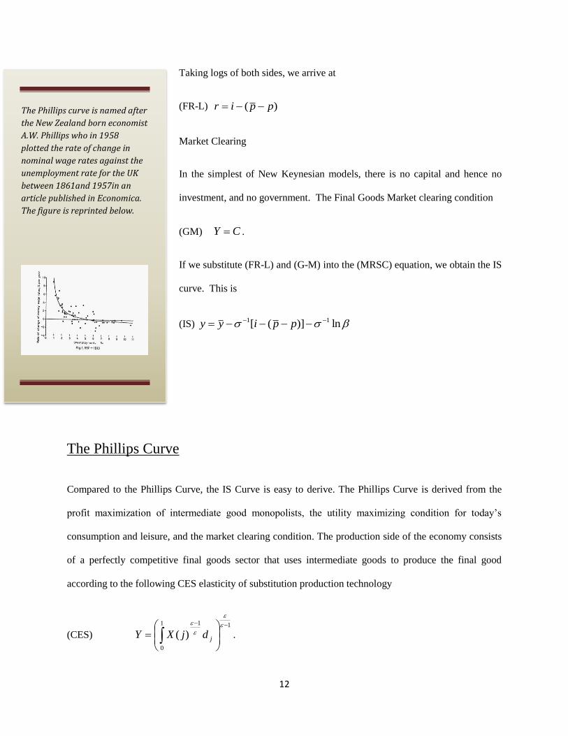
The Phillips curve is named after

the New Zealand born economist

A.W. Phillips who in 1958

plotted the rate of change in

nominal wage rates against the

unemployment rate for the UK

between 1861and 1957in an

article published in Economica.

The figure is reprinted below.

13

Below this is the intermediate good sector which consists of monopolies that set prices to maximize

profits subject to the demand for their product from the final goods sectors. Profit maximization by final

good producers yields the demand for intermediate good j

(X-Demand) YP

PjX

j

)(

Since the final good sector is perfectly competitive, firms must earn zero profits, namely,

(Zero-Profit) 1

0

)()( djjXjPPY

where the right hand side is the cost of buying the intermediate goods. Using (X-Demand) and (Zero

Profits), one can show that the Price of the final good is

(Price Index)

1

11

0

1)( jPP

To produce a given quantity of intermediated goods X requires H/A units of labor where A is TFP. More

specifically,

(X-Production) )()( jAHjX

Profit maximization of an intermediate producer yields the following the result that the optimal price is a

constant mark up over the marginal cost. Namely,

(Price equation) 1

)(

A

WjP

where W is that nominal wage rate.

14

The idea of the steady state, or full-employment level of output, Y , is the equilibrium quantity in the case

that all intermediate producers can re-optimize their prices in each period.

Critical to the New Keynesian theory is the existence of frictions. There are two approaches. The first

and the one adopted here is the assumption that not all intermediate firms are able to adjust their prices in

any given period. This harkens back to the work of Calvo (1983) and is referred to as the sticky price

assumption. An alternative that is attributed to the work of Mankiw and Reiss (2002) is the sticky

information assumption. With sticky information, not all intermediate good producers obtain the current

information. Those that do will set their prices upon the current information, but those that do not will set

it based on old information.

In the sticky price formulation, each intermediate good producer is has a random chance of being able to

change its price in the period. More specifically, with probability θ, a firm cannot change its price in the

period, and with probability (1-θ) the firm can change its price in the period. The inability of all firms to

reset prices is the key to having monetary shocks have real effects to the economy. If all firms could

adjust their prices in the period, then we would just have the standard Classical result. The nominal

interest rate and the inflation rate will adjust to keep the real interest rate constant. However, if some

firms cannot adjust their prices, then their goods will be relatively cheaper compared to the firms that can

raise their price. These stuck firms will see an increase in sales. They will no longer be maximizing

profits but because of their monopoly status do still realize some profitsGiven that the shock is

independently and identically distributed, the average time between price changes is 1/(1-θ). A firm that

is able to reset its price in the period must take this into account, that it may be many periods before they

are able to change their price again. Let us assume that a firm does this by minimizing the log price, zt,

that minimizes the expected discounted sum of square “errors” between the set price and the perfectly

flexible price. In particular, zt, is chosen to minimize

15

(Loss Function)

0

2* )()()(j

jttt

j

t pzEzL

In (Loss Function), p*t+j is the optimal price chosen in period t+j if prices were flexible. The idea is that

the firm, like the household, discounts the future at a rate β. Additionally, the probability that j periods

from now the firm has not able to reset its price is θj.

In a more rigorous formulation, the firm would choose its log price, zt, to maximize its expected profits.

In a certain sense, the loss function given by the quadratic function is intended to approximate the

expected profits.

To find the optimal reset price, we differentiate the (Loss Function) with respect zt and set the

0

* 0)()(2)('j

jttt

j

t pzEzL

Since the derivative is linear and separable in zt, this reduces to

(LF FONC)

0

*

0

)()(j

jtt

j

tj

j

t pEz

The left hand side summation is a geometric sum. For a geometric sum,

j

jx with x<1, the quantity is

equal to x1

1.

Hence, the left hand side of (LF FONC) reduces to

0

*)(1 j

jtt

jt pEz

.

Cross multiplying by (1-θβ), we arrive at

16

(ORP1)

0

*)()1(j

jtt

j

t pEz

There is a rather intuitive explanation for this expression. Specifically, the firm in setting its price today

will do so that it is keeping its price to the average expected optimal price.

The next step in deriving the New Keynesian Phillips curve is to characterize the optimal price in each

period, p*t+j. Here, we return to the (Pricing Equation). In logs, the (Pricing Equation) is

)1ln(ln* jtjtjt awp

Where w is the log of the nominal wage, W, and a is the log of the TFP, A. Their difference, w-a, is the

log of the marginal cost of producing an intermediate good. For convenience, let mct+j=wt+j-at+j and let

μ=lnε-ln(ε-1). Then

jtjt mcp*.

Next, we substitute the above equation into (ORP1). This is

(ORP2)

0

)()()1(j

jtt

j

t mcEz

The next step is to consider the law of motion for the aggregate price level. Returning to the (Price Index)

equation, it follows that the price level is a weighted average of the intermediate good producers pirces, a

fraction Given this stickiness, the law of motion for the price level is

(Price LM)

1

1

1*1

1 ]))(1([ ttt PPP .

Where does this come from? Think that in each period fraction (1-θ) intermediate good producers change

their price. That means today that (1-θ) firms set their price to Pt*. One period ago, another (1-θ) were

able to set their price to Pt-1*, and of these fraction θ did not change their price. Proceeding in this

17

fashion, we can write the current price level as a weighted average of the past prices set by the

monopolists. This is

(Recursive P)

1

1

1*21*

1

1*

1 ...])()1()()1())(1[(1t

PPPP ttt

We arrive at the (Price LM) by noting that the infinite sum of the terms on the right hand side of the

above equation starting with (1-θ)θ(P*t-1)

1-ε equals the aggregate price level at time t-1., i.e, Pt-1.

We next proceed by taking the First Order Taylor approximation of the (Recursive P) equation about its

steady state. This yields

*)*)(1()( 11 ttttt PPPPPP

Next we use the following trick. Define XXX tt lnln~

. Here the idea is that tX~

is the deviation of

the log of the variables from the steady state. Next, we can use the properties of logs to arrive at the

following relation X

XX

X

XX

X

XXXX ttt

tt

)1ln(lnlnln

~

. From here it is easy to

see that

)~

1( tt XXX

The First Order Taylor Approximation then is

*)~

1(*)1()~

1()~

1( 11 ttttt PPPPPPP

In a steady state *1 tt PPP . Using this result, the above equation simplifies to

*~

)1(~~

1 ttt PPP . And using the definition of XXX tt lnln~

, we arrive at

18

(aggregate price) *)1(1 ttt ppp .

As pt* is zt, in our notation, the aggregate price equation can be rewritten as

ttt zpp )1(1

From here we can solve for zt, namely,

(ORP from LM) )(1

11

ttt ppz

The next step returns to (ORP2). Here we make use of a result from ordinary stochastic difference

equations. Namely, if we have a first order stochastic difference equation of the form

1 tttt vbEaxv ,

then its solution is

ktt

j

k

t xEbav

0

. In our model,

vt = zt, xt=μ+mct, a=1-θβ, and b=θβ. The optimal reset price (ORP2) is actually the solution to the First

order stochastic difference equation given by

(ORP FOSDE) ))(1(1 tttt mcuzEz

From here, we substitute for the reset price in (ORP FOSDE) using (ORP from LM). This is

))(1()(1

)(1

111 tttttt mcuppEpp

The next step is to rewrite the above equation in terms of the inflation rate, πt. Recall that

1/ 1 ttt PP so that 1/1 ttt PP . If we take the log of both sides and use the result that

19

xx )1ln( , then 1 ttt pp . Rearranging the above equation so that we have expressions for πt

and πt+1 on each side, we arrive at

(NKPC MC form) )()1)(1(

1 ttttt pmcE

This says that today’s inflation is a function of the expected inflation rate and the excess of the marginal

cost over the price. The reason why inflation is a positive function of the gap between the marginal cost

and price level is that it implies a larger price reset for those firms that are able to reset prices.

The New Keynesian Phillips curve is usually expressed as a function of the output gap. To do this, we

first show that we can redefine the final good to be a linear function of the total labor supply, namely,

ttt NAY

Where 1

0

)( ttt djNN and 1

11

0

1)((

djjAA tt .

First, we use the demand equation and the intermediate production function. This is

YP

PjNjA

j

)()( . Using the price equation, this is

(1) YPjA

WjNjA

1

1

)()()(

Now solve for A(j) in the above equation and substitute it into the production function for the final good.

This yields

YP

WdjjAdjXY j

1

)()(11

0

111

0

1

, which implies

20

(2)

1)(

11

0

1

P

WdjjA

Now rearrange (1) so that we solve for N(j). This is

YP

WjAjN

1)()( 1

and intergrate over j. Then

(3) YP

WdjjAdjjN

1

)()(

1

0

1

1

0

. The left hand side of this equation is just N by the labor

market clearing condition. Now substitute (2) into (3) which yields

YdjjAN

1

11

0

1)( . This allows us to write

ttt NAY with

1

11

0

1)((

djjAA tt .

Now we go to the utility maximizing condition for labor and consumption. This is

(MRSC-labor)t

t

t

t

P

W

C

N

Using the goods market condition and the aggregate production function, we can rewrite (MRSC-Labor)

as

t

t

P

W

A

Y

Y

AY

)/(.

21

In logs, this is

(Actual output) tttt pway )(

Now we return to the (Price Equation) under the assumption that all firms can adjust their prices in the

period. Given the (Price index), it follows that under price flexibility, P(j)=P, provided that A(j) is the

same across firms. Thus,

1

11

PA

W.

Using the (MRSC-labor) condition, this can be rewritten as

1

)/(1

A

AYY, which in logs is

(Natural Rate)

1

1

1

nya

The superscript on the log of output indicates that this is the natural rate of output, i.e. the output for the

economy when all firms are able to adjust their prices.

To complete the derivation of the Phillips Curve we substitute wt-pt and at in the (NKPC MC form)

equation using the (Natural Rate) equation and (Actual Output) equation. This yields,

(NKPC) )())(1)(1(

1

n

tttt yyE

Monetary Policy

The final equation in the New Keynesian model is a monetary policy rule that determines the nominal

interest rate. Namely,

22

(Monetary Rule) ttytt yi

The term, υt, is a true shock to monetary policy. The monetary policy coefficients, y and are both

positive and are understood to be set by the monetary authority.

The monetary rule specified above is referred to as a Taylor rule, being named after the economist John

Taylor who first proposed it 1992. The above formulation is a simple version of the rule Taylor

proposed, which had the output gap, namely, yt-yn, instead of actual output, and the deviation of inflation

from its target, i.e., πt-π*, instead of the actual inflation rate in the monetary policy rule.

Solving the model

Solving the model is not trivial, even if the system is log linearized. For some very simplistic

systems, it is possible to solve using pen and paper, but mostly it is done on the computer.

Indeed, certain software packages are ideally suited for solving these log linearized systems.

Indeed, software packages such as DYNARE have made it relatively cheap for economists to

write a paper using a DSGE model.

Monetary Shocks: Developing Intuition

What is the effect of an unexpected decrease in the interest rate associated with the Taylor Rule?

The first thing this does is decrease the nominal interest rate, i. By the (IS) curve this will work

to increase demand provided that the interest rate rise is not perfectly offset by a rise in the price

level. And here is the critical feature of the New Keynesian model; with Sticky Prices following

Calvo (1983), this is not possible. Hence, the unexpected fall in the nominal interest rate

translates into a decrease in the real interest rate, and hence an increase in Aggregate Demand.

23

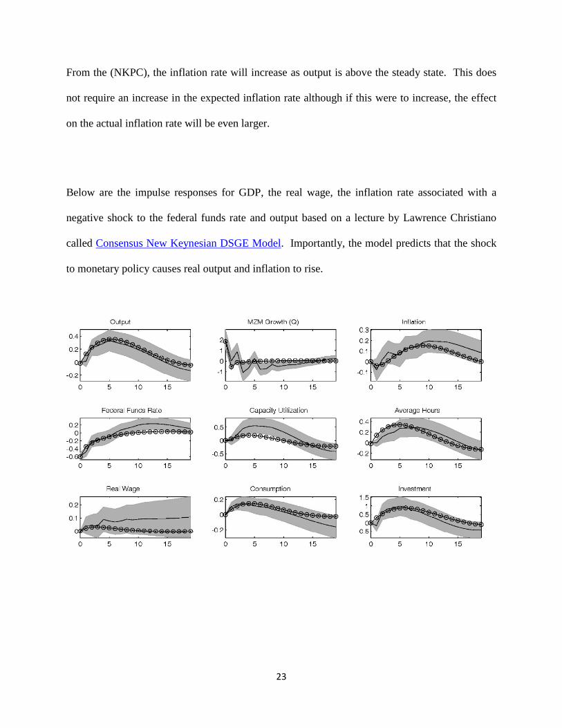
From the (NKPC), the inflation rate will increase as output is above the steady state. This does

not require an increase in the expected inflation rate although if this were to increase, the effect

on the actual inflation rate will be even larger.

Below are the impulse responses for GDP, the real wage, the inflation rate associated with a

negative shock to the federal funds rate and output based on a lecture by Lawrence Christiano

called Consensus New Keynesian DSGE Model. Importantly, the model predicts that the shock

to monetary policy causes real output and inflation to rise.

24

This is the general conclusion of the quantitative exercises, which in some ways are calibration exercises

and in other ways are estimation exercises. Practitioners of this approach typically assign parameters

based on other people’s work, and then estimate the other parameters typically using sophisticated

Econometric techniques. What is not obviously clear from these exercises is what these parameters are

being fitted to. Some fit the model to the impulse responses that they are trying to explain, which makes

these estimation exercises, or very bad calibration exercises.

Conclusion

The New Keynesian Model has become the dominant model choice of business cycle practicioners in the

last ten years. There are obvious reasons for this. First, it really is the only game in town for the purpose

of studying monetary economics. Second, despite the abandonment of the old Keynesian model in the last

part of the twentieth century, many economists never flinched from their beliefs that Keynes was right.

Although New Keynesian models have offered economists a way to study monetary policy all the while

of staying true to the principle of micro foundations, they are not subject to criticism. First, they are no

better than their RBC counterparts in predicting or understanding the Great Recessions. With maybe one

exception, they are silent about unemployment like their RBC counterparts. Additionally, they have had

moderate success in accounting for the persistence in output changes or price changes that are implied by

the VARS. For this they have added all sorts of extra parameters, many of which are not well grounded

in microeconomics.

25

References

Benigno, Pierpaolo. (2009) New Keynesian Economics: an AS-AD View. NBER Working Paper 14824.

Calvo (1983)

Sargent, Thomas and Neil Wallace 1975. Rational Expectations, the Optimal Monetary Instrument, and

the Optimal Money Supply Rule. Journal of Political Economy 83, 241-254.

Taylor, John. 1979. Staggered Wage Setting in a Macro Model. American Economic Review 69(2): 108-

113.

Chari, V, P. Kehoe and E. McGrattan.

26

Sims, Christopher (1980). "Macroeconomics and Reality". Econometrica 48 (1): 1–48.

Extensions

To rewrite the (GM) equation in terms of logs, one needs to make use of some other properties of

logarithms.

Define XXX tt lnln~

. Here the idea is that tX~

is the deviation of the log of the variables from the

steady state. Next, we can use the properties of logs to arrive at the following relation

X

XX

X

XX

X

XXXX ttt

tt

)1ln(lnlnln

~

. From here it is easy to see that

)~

1( tt XXX

Now we shall apply this result to the goods market clearing condition. This yields

)~

1()~

1()~

1( ttt GGCCYY

Next apply the distributive law and make use of the steady state goods market clearing condition. In doing

this, the above equation simplifies to

ttt GGCCYY~~~

Let YCsc / and YGsg / . Then we can rewrite the above equation as tgtct GsCsY~~~

. And now

applying the definition of our variables with the tildes, we arrive at

)()( ggsccsyy gc

The last step in deriving the IS Equation is to substitute the above equation and Equation (FE-L) into the

(EE-L). This yields

27

(IS) )(ˆ)]([ˆ ggsppisyy gc

Where

lncs ,

c

c

ss ˆ

gcg sss ˆ . Note that in (IS), when the price level is below its steady state,

output will be above its steady state. The (IS) equation here intuitively can be thought of as an aggregate

demand curve.