Business Calculus Math 1431 - LSU Mathematicsdavidson/m1550/Unit2_6.pdfSection 2.6: The Derivative...
88
Section 2.6: The Derivative Business Calculus - p. 1/44 Business Calculus Math 1431 Unit 2.6 The Derivative Mathematics Department Louisiana State University
-
Upload
hoangkhuong -
Category
Documents
-
view
217 -
download
0
Transcript of Business Calculus Math 1431 - LSU Mathematicsdavidson/m1550/Unit2_6.pdfSection 2.6: The Derivative...

Section 2.6: The Derivative Business Calculus - p. 1/44
Business CalculusMath 1431
Unit 2.6The DerivativeMathematics Department
Louisiana State University

IntroductionIntroductionThe TangentProblemThe Slope?Secant linesSmall hThe main ideaAn animationSlope of TangentExample
Section 2.6: The Derivative Business Calculus - p. 2/44
Introduction

IntroductionIntroductionThe TangentProblemThe Slope?Secant linesSmall hThe main ideaAn animationSlope of TangentExample
Section 2.6: The Derivative Business Calculus - p. 3/44
Introduction
In an earlier lecture we considered the idea offinding the average rate of change of some quan-tity Q(t) over a time interval [t1, t2] and askedwhat would happen when the time interval becamesmaller and smaller. This led to the notion of limits,which we have examined in the previous two lec-tures. In this section we return to our study of av-erage rates of change and apply what we learnedabout limits. This leads directly to the derivative.It turns out that the derivative has an equivalent(purely) mathematical formulation: that of findingthe line tangent to a curve at some point. This iswhere we will start.
IntroductionIntroductionThe TangentProblemThe Slope?Secant linesSmall hThe main ideaAn animationSlope of TangentExample
Section 2.6: The Derivative Business Calculus - p. 4/44
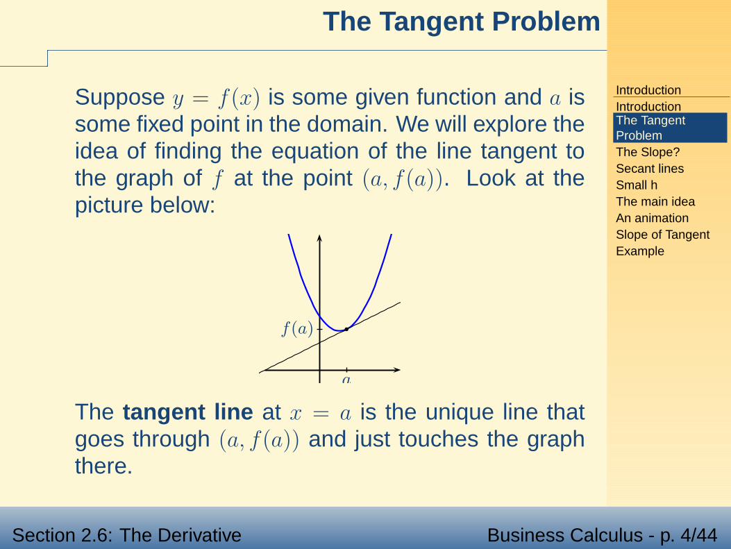
The Tangent Problem
Suppose y = f(x) is some given function and a issome fixed point in the domain. We will explore theidea of finding the equation of the line tangent tothe graph of f at the point (a, f(a)). Look at thepicture below:
a
f(a)
The tangent line at x = a is the unique line thatgoes through (a, f(a)) and just touches the graphthere.

IntroductionIntroductionThe TangentProblemThe Slope?Secant linesSmall hThe main ideaAn animationSlope of TangentExample
Section 2.6: The Derivative Business Calculus - p. 5/44
The Slope?
Recall the an equation of the line is determinedonce we know a point P and the slope m. IfP = (a, f(a)) then the equation of the line tangentto the curve will take the form
y − f(a) = m(x − a)
for some slope m that we have to determine.
How do we determine theslope of the tangent line?
We will do so by a limiting process.

IntroductionIntroductionThe TangentProblemThe Slope?Secant linesSmall hThe main ideaAn animationSlope of TangentExample
Section 2.6: The Derivative Business Calculus - p. 6/44
Secant lines
Given the graph of a function y = f(x) we call asecant line a line that connects two points on agraph.
In the graph to the right a redline joins the points (a, f(a)) and(a+h, f(a+h). ( Think of h as arelatively small number.) a
f(a)
a + h
f(a + h)
Now, what is the slope of the secant line? Thechange in y is ∆y = f(a+h)−f(a) and the changein x is ∆x = a + h − a = h. So the slope of thesecant line is:
∆y
∆x=
f(a + h) − f(a)
h.

IntroductionIntroductionThe TangentProblemThe Slope?Secant linesSmall hThe main ideaAn animationSlope of TangentExample
Section 2.6: The Derivative Business Calculus - p. 7/44
Small h
The following graph illustrates what happens whenwe choose smaller values of h. Notice how the se-cant lines get closer to the tangent line.
a
f(a)
IntroductionIntroductionThe TangentProblemThe Slope?Secant linesSmall hThe main ideaAn animationSlope of TangentExample
Section 2.6: The Derivative Business Calculus - p. 8/44
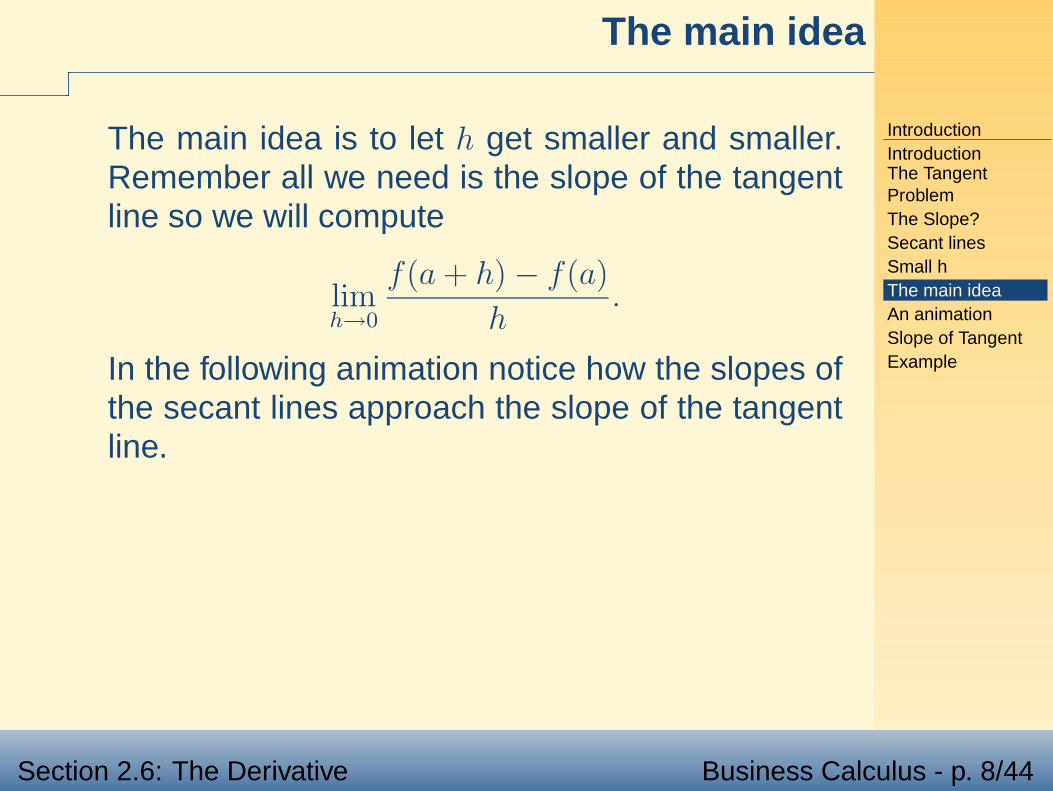
The main idea
The main idea is to let h get smaller and smaller.Remember all we need is the slope of the tangentline so we will compute
limh→0
f(a + h) − f(a)
h.
In the following animation notice how the slopes ofthe secant lines approach the slope of the tangentline.

IntroductionIntroductionThe TangentProblemThe Slope?Secant linesSmall hThe main ideaAn animationSlope of TangentExample
Section 2.6: The Derivative Business Calculus - p. 9/44
Convergence of Secant Lines: An animation
Notice how the secant line and hence its slopes converge to the
tangent line.

IntroductionIntroductionThe TangentProblemThe Slope?Secant linesSmall hThe main ideaAn animationSlope of TangentExample
Section 2.6: The Derivative Business Calculus - p. 10/44
Slope of the Tangent Line
Since the slope of the secant lines are given by theformula
f(a + h) − f(a)
h,
the slope of the tangent line is given by
limh→0
f(a + h) − f(a)
h,
when this exists. We will call this number thederivative of f at a and denote it f ′(a). Thus
The derivative of f at x = a is given by
f ′(a) = limh→0
f(a + h) − f(a)
h.

IntroductionIntroductionThe TangentProblemThe Slope?Secant linesSmall hThe main ideaAn animationSlope of TangentExample
Section 2.6: The Derivative Business Calculus - p. 11/44
Example
To illustrate some of these ideas let’s consider thefollowing example:
Example 1: Let f(x) = x2 and fix a = 1. Computethe slope of the secant line that connects (a, f(a))and (a + h, f(a + h) for■ h = 1
■ h = .5
■ h = .1
■ h = .01
Compute the derivative of f at x = 1, i.e. f ′(1).Finally, find the equation of the line tangent to thegraph of f(x) = x2 and x = 1.

IntroductionIntroductionThe TangentProblemThe Slope?Secant linesSmall hThe main ideaAn animationSlope of TangentExample
Section 2.6: The Derivative Business Calculus - p. 12/44
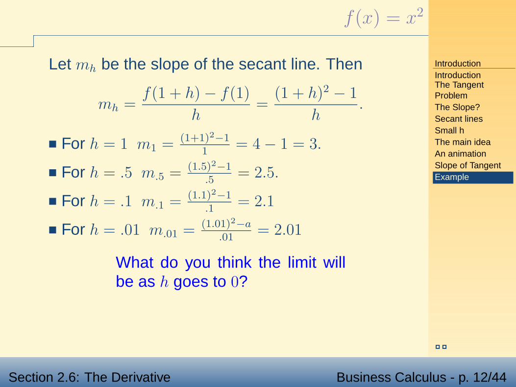
f(x) = x2
Let mh be the slope of the secant line. Then
mh =f(1 + h) − f(1)
h=
(1 + h)2 − 1
h.
■ For h = 1 m1 = (1+1)2−11
= 4 − 1 = 3.
■ For h = .5 m.5 = (1.5)2−1.5
= 2.5.
■ For h = .1 m.1 = (1.1)2−1.1
= 2.1
■ For h = .01 m.01 = (1.01)2−a
.01= 2.01
IntroductionIntroductionThe TangentProblemThe Slope?Secant linesSmall hThe main ideaAn animationSlope of TangentExample
Section 2.6: The Derivative Business Calculus - p. 12/44
f(x) = x2
Let mh be the slope of the secant line. Then
mh =f(1 + h) − f(1)
h=
(1 + h)2 − 1
h.
■ For h = 1 m1 = (1+1)2−11
= 4 − 1 = 3.
■ For h = .5 m.5 = (1.5)2−1.5
= 2.5.
■ For h = .1 m.1 = (1.1)2−1.1
= 2.1
■ For h = .01 m.01 = (1.01)2−a
.01= 2.01
What do you think the limit willbe as h goes to 0?

IntroductionIntroductionThe TangentProblemThe Slope?Secant linesSmall hThe main ideaAn animationSlope of TangentExample
Section 2.6: The Derivative Business Calculus - p. 13/44
f(x) = x2
The limit is the derivative. We compute
f ′(1) = limh→0
f(a + h) − f(a)
h
= limh→0
(1 + h)2 − 1
h
= limh→0
1 + 2h + h2 − 1
h
= limh→0
2h + h2
h= lim
h→02 + h = 2.
Therefore the slope of the tangent line is m = 2.

IntroductionIntroductionThe TangentProblemThe Slope?Secant linesSmall hThe main ideaAn animationSlope of TangentExample
Section 2.6: The Derivative Business Calculus - p. 14/44
f(x) = x2
The equation of the tangent line is now an easymatter. The slope m is 2 and the point P that theline goes through is (1, f(1)) = (1, 1). Thus, we get
y − 1 = 2(x − 1)
ory = 2x − 1.
On the next slide we give a graphical representa-tion of what we have just computed.

IntroductionIntroductionThe TangentProblemThe Slope?Secant linesSmall hThe main ideaAn animationSlope of TangentExample
Section 2.6: The Derivative Business Calculus - p. 15/44
f(x) = x2

IntroductionIntroductionThe TangentProblemThe Slope?Secant linesSmall hThe main ideaAn animationSlope of TangentExample
Section 2.6: The Derivative Business Calculus - p. 15/44
f(x) = x2
Here h = 1 and the secant line goes through thepoints (1, 1) and (2, 4)

IntroductionIntroductionThe TangentProblemThe Slope?Secant linesSmall hThe main ideaAn animationSlope of TangentExample
Section 2.6: The Derivative Business Calculus - p. 15/44
f(x) = x2
Here h = .5 and the secant line goes through thepoints (1, 1) and (1.5, 2.25)

IntroductionIntroductionThe TangentProblemThe Slope?Secant linesSmall hThe main ideaAn animationSlope of TangentExample
Section 2.6: The Derivative Business Calculus - p. 15/44
f(x) = x2
Here h = .1 and the secant line goes through thepoints (1, 1) and (1.1, 1.21)

IntroductionIntroductionThe TangentProblemThe Slope?Secant linesSmall hThe main ideaAn animationSlope of TangentExample
Section 2.6: The Derivative Business Calculus - p. 15/44
f(x) = x2
Here h = .01 and the secant line goes through thepoints (1, 1) and (1.01, 1.0201)

Rates of ChangeRates of changeVelocityExample
Section 2.6: The Derivative Business Calculus - p. 16/44
Rates of Change
Rates of ChangeRates of changeVelocityExample
Section 2.6: The Derivative Business Calculus - p. 17/44
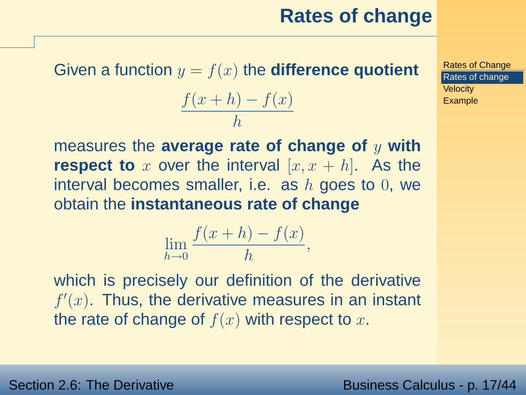
Rates of change
Given a function y = f(x) the difference quotient
f(x + h) − f(x)
h
measures the average rate of change of y withrespect to x over the interval [x, x + h]. As theinterval becomes smaller, i.e. as h goes to 0, weobtain the instantaneous rate of change
limh→0
f(x + h) − f(x)
h,
which is precisely our definition of the derivativef ′(x). Thus, the derivative measures in an instantthe rate of change of f(x) with respect to x.

Rates of ChangeRates of changeVelocityExample
Section 2.6: The Derivative Business Calculus - p. 18/44
Velocity
If s(t) is the distance travelled by an object (yourcar for instance) as a function of time t then thequantity
s(t + h) − s(t)
h
is the average rate of change of distance over thetime interval [t, t + h]. This is none other than youraverage velocity. The quantity
limh→0
s(t + h) − s(t)
h
is the instantaneous rate of change: This is noneother than your velocity which you would read fromyour speedometer. Thus your speedometer can bethought of as a derivative machine.
Rates of ChangeRates of changeVelocityExample
Section 2.6: The Derivative Business Calculus - p. 19/44
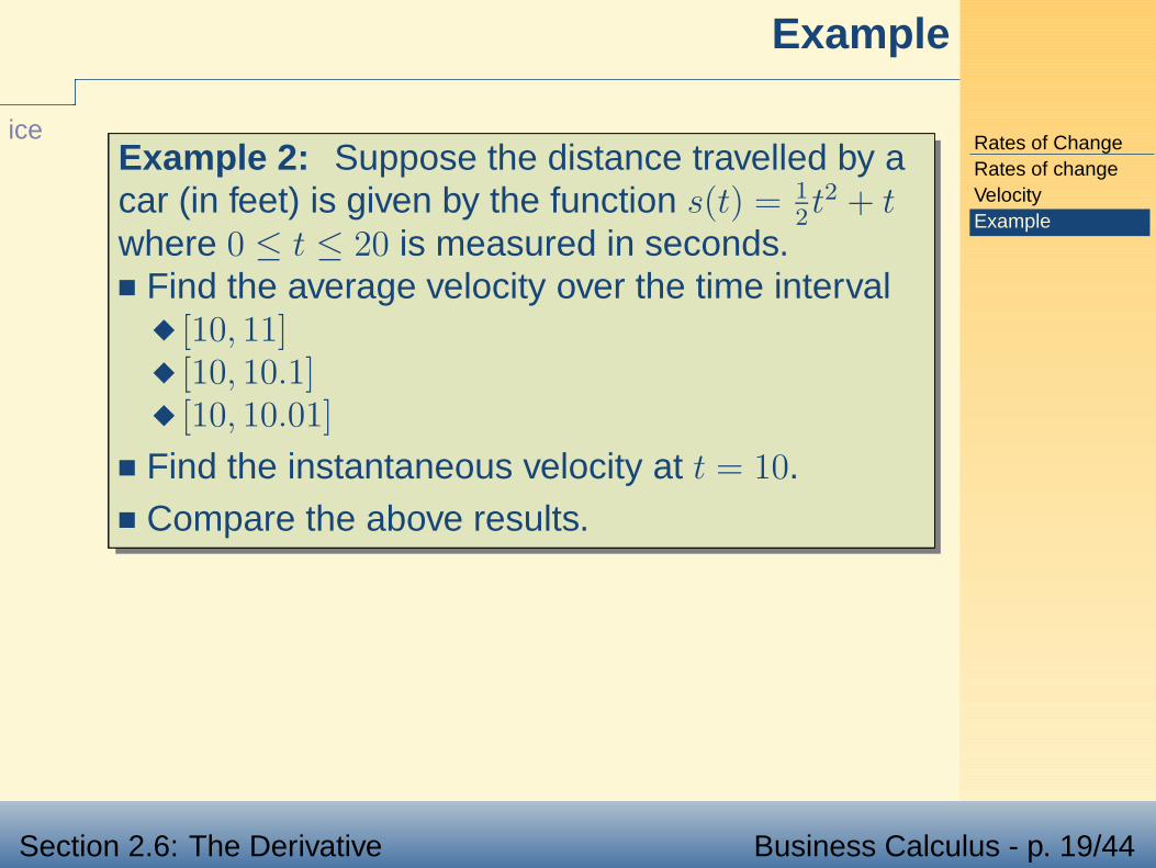
Example
iceExample 2: Suppose the distance travelled by acar (in feet) is given by the function s(t) = 1
2t2 + t
where 0 ≤ t ≤ 20 is measured in seconds.■ Find the average velocity over the time interval
◆ [10, 11]◆ [10, 10.1]◆ [10, 10.01]
■ Find the instantaneous velocity at t = 10.■ Compare the above results.

Rates of ChangeRates of changeVelocityExample
Section 2.6: The Derivative Business Calculus - p. 20/44
s(t) = 1
2t2 + t
■ The average velocity over the given time intervalsare:
◆s(11)−s(10)
11−10= 1
2(11)2 + 11 − (1
2(10)2 + 10) = 11.5
(ft/sec)
◆s(10.1)−s(10)
10.1−10= 1.105
.1= 11.05 (ft/sec)
◆s(10.01)−s(10)
10.01−10= 1.1005
.01= 11.005 (ft/sec)

Rates of ChangeRates of changeVelocityExample
Section 2.6: The Derivative Business Calculus - p. 21/44
s(t) = 1
2t2 + t
■ We could probably guess that the instantaneousvelocity at t = 10 is 11 (ft/sec). But lets calculatethis using the definition
s′(t) = limh→0
s(t + h) − s(t)
h
= limh→0
12(t + h)2 + (t + h) − (1
2t2 + t)
h
= limh→0
12(t2 + 2th + h2) + t + h − 1
2t2 − t
h
= limh→0
th + 12h2 + h
h
= limh→0
t +1
2h + 1 = t + 1.

Rates of ChangeRates of changeVelocityExample
Section 2.6: The Derivative Business Calculus - p. 22/44
s(t) = 1
2t2 + t
Notice that we have calculated the derivative at anypoint t:
s′(t) = t + 1.
We now evaluate at t = 10 to get
s′(10) = 11
just as we expected.
The average velocity over the time intervals[10, 10 + h] for h = 1, h = .1 and h = .01 becomecloser to the instantaneous velocity at t = 10. Thisis as we should expect.

DiffereniationNotationAn outlineExampleExampleDo not despair!
Section 2.6: The Derivative Business Calculus - p. 23/44
Finding the derivative of a functionusing the definition

DiffereniationNotationAn outlineExampleExampleDo not despair!
Section 2.6: The Derivative Business Calculus - p. 24/44
Notation
Differential calculus has various ways of denotingthe derivative, each with their own advantages.We have used the prime notation , f ′(x) (read: "fprime of x"), to denote the derivative of y = f(x).You will also see y′ written when it is clear y = f(x).The prime notation is simple, quick to write, but notvery inspiring.

DiffereniationNotationAn outlineExampleExampleDo not despair!
Section 2.6: The Derivative Business Calculus - p. 25/44
Another notation is
df
dxor
dy
dx.
This notation is much more suggestive. Recall thatthe derivative is the limit of the difference quotient∆y
∆x: the change in y over the change in x. The
notation "dy" or "df " is used to suggest the instan-taneous change in y after the limit is taken and like-wise for dx. One must not read too much into thisnotation. df
dxis not a fraction but the limit of a frac-
tion.
There are other notations that are in use but theseare the two most common.

DiffereniationNotationAn outlineExampleExampleDo not despair!
Section 2.6: The Derivative Business Calculus - p. 26/44
An outline
To compute the derivative df
dx= f ′(x) of a function
y = f(x) using the definition follow the steps:
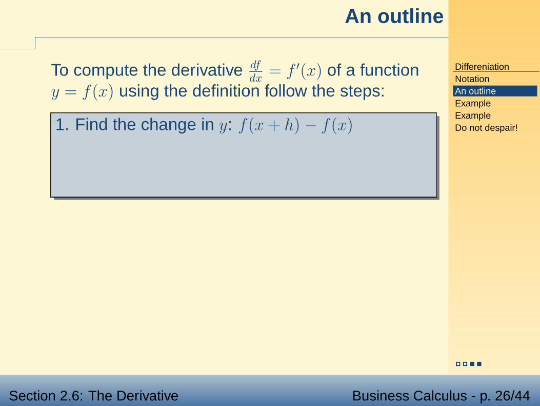
DiffereniationNotationAn outlineExampleExampleDo not despair!
Section 2.6: The Derivative Business Calculus - p. 26/44
An outline
To compute the derivative df
dx= f ′(x) of a function
y = f(x) using the definition follow the steps:
1. Find the change in y: f(x + h) − f(x)

DiffereniationNotationAn outlineExampleExampleDo not despair!
Section 2.6: The Derivative Business Calculus - p. 26/44
An outline
To compute the derivative df
dx= f ′(x) of a function
y = f(x) using the definition follow the steps:
1. Find the change in y: f(x + h) − f(x)
2. Compute f(x+h)−f(x)h

DiffereniationNotationAn outlineExampleExampleDo not despair!
Section 2.6: The Derivative Business Calculus - p. 26/44
An outline
To compute the derivative df
dx= f ′(x) of a function
y = f(x) using the definition follow the steps:
1. Find the change in y: f(x + h) − f(x)
2. Compute f(x+h)−f(x)h
3. Determine limh→0f(x+h)−f(x)
h.

DiffereniationNotationAn outlineExampleExampleDo not despair!
Section 2.6: The Derivative Business Calculus - p. 27/44
Example
iceExample 3: Find the derivative of y = x3 − x.

DiffereniationNotationAn outlineExampleExampleDo not despair!
Section 2.6: The Derivative Business Calculus - p. 27/44
Example
iceExample 3: Find the derivative of y = x3 − x.
Let f(x) = x3 − x. Then
f(x + h) − f(x) = (x + h)3 − (x + h) − (x3 − x)
= x3 + 3x2h + 3xh2 + h3
−x − h − x3 + x
= 3x2h + 3xh2 + h3 − h
Next we get
f(x + h) − f(x)
h=
3x2h + 3xh2 + h3 − h
h
= 3x2 + 3xh + h2 − 1
Finally, dy
dx= limh→0 3x2 + 3xh + h2 − 1 = 3x2 − 1.
DiffereniationNotationAn outlineExampleExampleDo not despair!
Section 2.6: The Derivative Business Calculus - p. 28/44
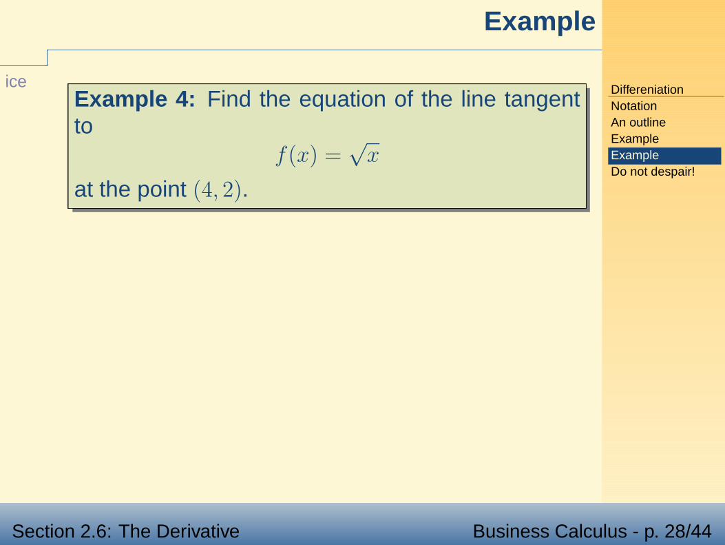
Example
iceExample 4: Find the equation of the line tangentto
f(x) =√
x
at the point (4, 2).

DiffereniationNotationAn outlineExampleExampleDo not despair!
Section 2.6: The Derivative Business Calculus - p. 29/44
f(x) =√
x
We need the slope of the tangent line at this point.This is f ′(4).
f′(4) = lim
h→0
f(4 + h) − f(4)
h
= limh→0
√
4 + h − 2
h
= limh→0
√
4 + h − 2
h
√
4 + h + 2√
4 + h + 2
= limh→0
4 + h − 4
h(√
4 + h + 2)
= limh→0
1√
4 + h + 2=
1
4.

DiffereniationNotationAn outlineExampleExampleDo not despair!
Section 2.6: The Derivative Business Calculus - p. 30/44
f ′(4) = 1
4and P = (4, 2)
Given a point and a slope we compute the line:
y − 2 =1
4(x − 4)
or
y =1
4x + 1.

DiffereniationNotationAn outlineExampleExampleDo not despair!
Section 2.6: The Derivative Business Calculus - p. 31/44
Do not despair!
Admittedly, the calculation of a derivative using thedefinition can be tedious. However, in the nextchapter we will discuss a set of rules for differenti-ation that will allow us to calculate the derivative ofmany commonly encountered functions very eas-ily. Nevertheless, it is important that you under-stand the definition and the underlying meaning ofthe derivative; at times, it will be necessary to comeback to it.

ContinuityReformulationDifferentiabilityProofContinuiity
Section 2.6: The Derivative Business Calculus - p. 32/44
Differentiation and Continuity

ContinuityReformulationDifferentiabilityProofContinuiity
Section 2.6: The Derivative Business Calculus - p. 33/44
Reformulation of Continuity
In the last section we discussed the meaning ofcontinuity. Recall a function y = f(x) is continu-ous at a point a if f(a) is defined and
limx→a
f(x) = f(a).
If we let x = a + h then x approaches a if h ap-proaches 0. This observations allows us the givean equivalent definition for continuity: f(a) is de-fined and
limh→0
f(a + h) − f(a) = 0.

ContinuityReformulationDifferentiabilityProofContinuiity
Section 2.6: The Derivative Business Calculus - p. 34/44
Differentiable functions are Continuous
A function is said to be differentiable at a pointx = a if f ′(a) exists. This means that the limitlimh→0
f(a+h)−f(a)h
exists. We say f is differentiableon an interval (a, b) if it is differentiable at everypoint in the interval.
Notice the next theorem:
Theorem: A function that is differentiable at apoint x = a is continuous there.
We have not been proving many theorems but thisone is easy and short enough that we will do so onthe next slide.

ContinuityReformulationDifferentiabilityProofContinuiity
Section 2.6: The Derivative Business Calculus - p. 35/44
Proof
Proof: To say f is differentiable at x = a means
limh→0
f(a + h) − f(a)
h
exists and is a finite number, denoted f ′(a). Thus
limh→0
(f(a + h) − f(a)) = limh→0
f(a + h) − f(a)
h· h
= limh→0
f(a + h) − f(a)
h· lim
h→0(h)
= f ′(a) · 0 = 0.
This means that f is continuous at x = a.

ContinuityReformulationDifferentiabilityProofContinuiity
Section 2.6: The Derivative Business Calculus - p. 36/44
Continuity does not imply Differentiability
We must not read something that is not in this theo-rem. Though a differentiable function is necessarilycontinuous a continuous function is not necessarilydifferentiable. Consider this classic example:
y = |x| .At x = 0 there are several lines that just touch thegraph at (0, 0); it is not unique.
Remember, tangent lines are unique and sincey = |x| has no unique tangent line it is not differ-entiable at x = 0.

ContinuityReformulationDifferentiabilityProofContinuiity
Section 2.6: The Derivative Business Calculus - p. 37/44
y = |x| at x = 0
Consider what happens here in terms of the defini-tion:
y′(0) = limh→0
|0 + h| − 0
h
= limh→0
|h|h
.
Now, to compute this limit we will consider the leftand right-hand limits.
ContinuityReformulationDifferentiabilityProofContinuiity
Section 2.6: The Derivative Business Calculus - p. 38/44
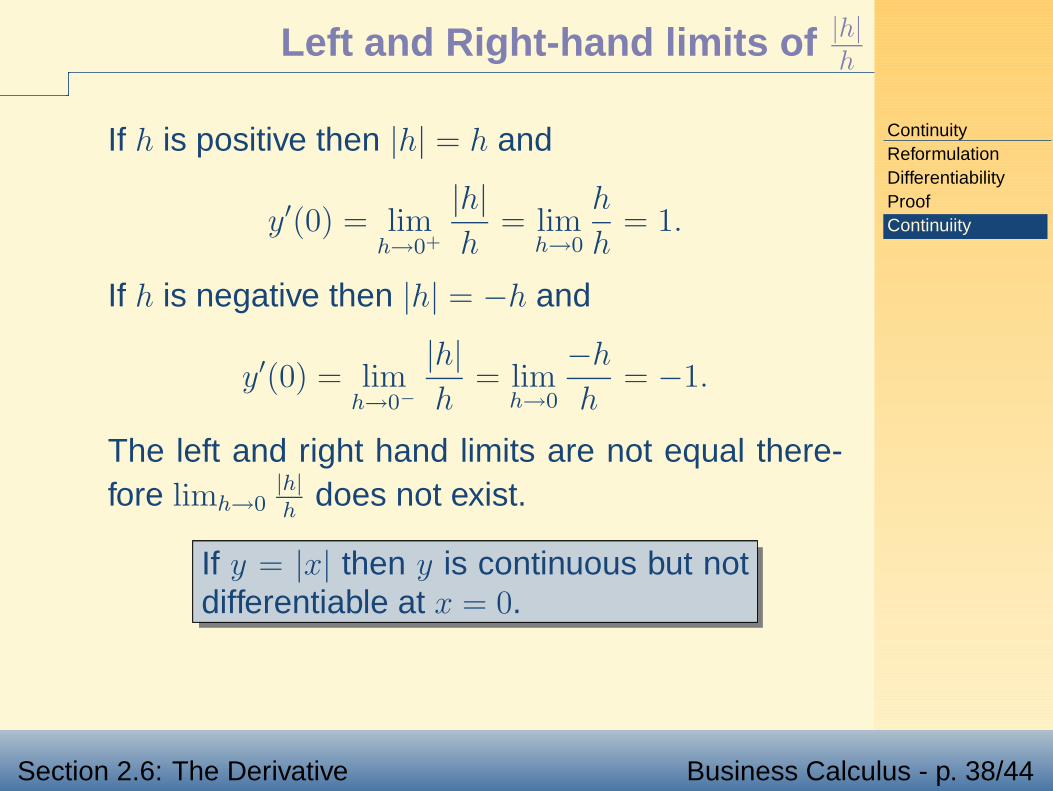
Left and Right-hand limits of |h|h
If h is positive then |h| = h and
y′(0) = limh→0+
|h|h
= limh→0
h
h= 1.
If h is negative then |h| = −h and
y′(0) = limh→0−
|h|h
= limh→0
−h
h= −1.
The left and right hand limits are not equal there-fore limh→0
|h|h
does not exist.
If y = |x| then y is continuous but notdifferentiable at x = 0.

SummarySummary
Section 2.6: The Derivative Business Calculus - p. 39/44
Summary

SummarySummary
Section 2.6: The Derivative Business Calculus - p. 40/44
Summary
This section is very important and likely new tomany students in this course. Here are some keyconcepts to master.

SummarySummary
Section 2.6: The Derivative Business Calculus - p. 40/44
Summary
This section is very important and likely new tomany students in this course. Here are some keyconcepts to master.
■ The definition of the derivative:f ′(x) = limh→0
f(x+h)−f(x)h
.

SummarySummary
Section 2.6: The Derivative Business Calculus - p. 40/44
Summary
This section is very important and likely new tomany students in this course. Here are some keyconcepts to master.
■ The definition of the derivative:f ′(x) = limh→0
f(x+h)−f(x)h
.
■ The meaning: The derivative of a functionrepresents the instantaneous rate of change of f
as a function of x.

SummarySummary
Section 2.6: The Derivative Business Calculus - p. 40/44
Summary
This section is very important and likely new tomany students in this course. Here are some keyconcepts to master.
■ The definition of the derivative:f ′(x) = limh→0
f(x+h)−f(x)h
.
■ The meaning: The derivative of a functionrepresents the instantaneous rate of change of f
as a function of x.■ Primary Applications: Tangent lines, velocity

SummarySummary
Section 2.6: The Derivative Business Calculus - p. 40/44
Summary
This section is very important and likely new tomany students in this course. Here are some keyconcepts to master.
■ The definition of the derivative:f ′(x) = limh→0
f(x+h)−f(x)h
.
■ The meaning: The derivative of a functionrepresents the instantaneous rate of change of f
as a function of x.■ Primary Applications: Tangent lines, velocity■ Computation of the derivative.

SummarySummary
Section 2.6: The Derivative Business Calculus - p. 40/44
Summary
This section is very important and likely new tomany students in this course. Here are some keyconcepts to master.
■ The definition of the derivative:f ′(x) = limh→0
f(x+h)−f(x)h
.
■ The meaning: The derivative of a functionrepresents the instantaneous rate of change of f
as a function of x.■ Primary Applications: Tangent lines, velocity■ Computation of the derivative.■ The connection between continuity and
differentiation.

SummarySummary
Section 2.6: The Derivative Business Calculus - p. 40/44
Summary
This section is very important and likely new tomany students in this course. Here are some keyconcepts to master.
■ The definition of the derivative:f ′(x) = limh→0
f(x+h)−f(x)h
.
■ The meaning: The derivative of a functionrepresents the instantaneous rate of change of f
as a function of x.■ Primary Applications: Tangent lines, velocity■ Computation of the derivative.■ The connection between continuity and
differentiation.■ Notation: y′ or dy
dx.

In-Class ExercisesICEICEICE
Section 2.6: The Derivative Business Calculus - p. 41/44
In-Class Exercises
In-Class ExercisesICEICEICE
Section 2.6: The Derivative Business Calculus - p. 42/44
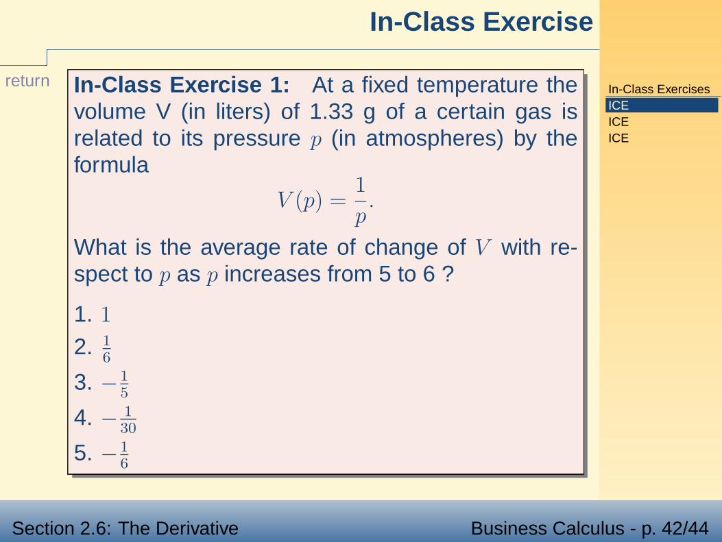
In-Class Exercise
return In-Class Exercise 1: At a fixed temperature thevolume V (in liters) of 1.33 g of a certain gas isrelated to its pressure p (in atmospheres) by theformula
V (p) =1
p.
What is the average rate of change of V with re-spect to p as p increases from 5 to 6 ?
1. 1
2. 16
3. −15
4. − 130
5. −16

In-Class ExercisesICEICEICE
Section 2.6: The Derivative Business Calculus - p. 43/44
In-Class Exercise
returnIn-Class Exercise 2: Use the definition of thederivative to find y′ if
y = 4x2 − x.
1. 4x2 − 1
2. 8x − 1
3. 8x
4. 4x2 − x
5. None of the above

In-Class ExercisesICEICEICE
Section 2.6: The Derivative Business Calculus - p. 44/44
In-Class Exercise
returnIn-Class Exercise 3: Find the equation of the linetangent to
y = x2 + x
at the point (1, 2).
1. y = 3x − 1
2. y = 3x − 5
3. y = 2x
4. y = 2x − 3
5. None of the above

![Cambridge University Press, Financial Calculus - An Introduction to Derivative Pricing [1996 Isbn0521552893]](https://static.fdocuments.in/doc/165x107/55cf8f9b550346703b9de9a5/cambridge-university-press-financial-calculus-an-introduction-to-derivative.jpg)