Building Lexicons Jae Dong Kim Matthias Eck. Building Lexicons lIntroduction lPrevious Work...
69
Building Lexicons Jae Dong Kim Matthias Eck
-
Upload
imogen-gibson -
Category
Documents
-
view
221 -
download
2
Transcript of Building Lexicons Jae Dong Kim Matthias Eck. Building Lexicons lIntroduction lPrevious Work...

Building Lexicons
Jae Dong KimMatthias Eck

Building Lexicons
Introduction Previous Work Translation Model Decomposition Reestimated Models Parameter Estimation Method A Method B Method C Evaluation Conclusion

Building Lexicons
Introduction Previous Work Translation Model Decomposition Reestimated Models Parameter Estimation Method A Method B Method C Evaluation Conclusion

Definitions
Translational equivalence: A relation that holds between two expressions with the same meaning, where two expressions are in different languages.
Statistical Translation Models: statistical models of translational equivalence
Empirical estimation of statistical translation models is typically based on parallel texts or bitexts
Word-to-Word Lexicon A list of word pairs (source word, target word ) Bidirectional Probabilistic word-to-word lexicon (source word, target word,
prob.)

Additional Universal Property
Translation models benefit from the best of both the empiricist and rationalist traditions
Models to be proposed Most word tokens translate to only one word token.
Approximated by one-to-one assumption - Method A Most text segments are not translated word for word. Explicit
Noise Model - Method B Different linguistic objects have statistically different behavior
in translation. Translation models on different word classes. - Method C
Human judgment has shown that each of three estimation biases improves translation model accuracy over a baseline knowledge-free model

Applications of Translation Models
Where word order is not important Cross-language information retrieval Multilingual document filtering Computer-assisted language learning Certain machine-assisted translation tools Concordancing for bilingual lexicography Corpus linguistics “crummy” machine translation
Where word order is important Speech transcription for translation Bootstrapping of OCR systems for new languages Interactive translation Fully automatic high-quality machine translation
Advantages of translation models
Compared to handcrafted models The possibility of better coverage The possibility of frequent updates More accurate information about relative importance of
different translations
Q’ T QiIRDB
IR
Uniform Importance?

Building Lexicons
Introduction Previous Work Translation Model Decomposition Reestimated Models Parameter Estimation Method A Method B Method C Evaluation Conclusion

Models of Co-occurrence
Intuition: words that are translations of each other are more likely to appear in corresponding bitext regions than other pairs of words.
A boundary-based model: assumes that both halves of the bitext have been segmented into s segments, so that segment Ui in one half of the bitext and segment Vi in the other half are mutual translations, 1<=i<=s Co-occurrence count by Brown et al
Co-occurrence count by Melamed
cooc(u,v) ei(u)f i(v)i1
s
cooc(u,v) min[ei(u), f i(v)]i1
s

Nonprobabilistic Translation Lexicons (1)
Summary of non-probabilistic translation lexicon algorithms1. Choose a similarity function S between word types in L1 and
word types L2
2. Compute association scores S(u,v) for a set of word type pairs (u,v) (L1 x L2) that occur in training data
3. Sort the word pairs in descending order of their association scores
4. Discard all word pairs for which S(u,v) is less than a chosen threshold. The remaining word pairs become the entries in the translation lexicon
1. Main difference: choice of similarity function2. Those functions are based on a model of co-
occurrence with some linguistically motivated filtering

Nonprobabilistic Translation Lexicons (2)
Problem: independence assumption in step 2 Models of translational equivalence that are ignorant of
indirect association have “a tendency … to be confused by collocates”
If all the entries in a translation lexicon are sorted by their association scores, the direct associations will be very dense near the top of the list, and sparser towards the bottom
He nods his head
Il hoche la tete
Direct association Indirect association

Nonprobabilistic Translation Lexicons (3)
The very top of the list can be over 98% correct - Gale and Church (1991) Gleaned lexicon entries for about 61% of the word tokens in a
sample of 800 English sentences Selected only entries with high association score 61% word tokens represent 4.5%word types
71.6% precision with top 23.8% of noun-noun entries - Fung(1995)
Automatic acquisition of 6,517 lexicon entries with 86% precision from 3.3-million-word corpus - Wu & Xia (1994) 19% recall Weighted precision: in {(E1,C1,0.533), (E1,C2,0.277),
(E1,C3,0.190)}, if (E1,C3,0.190) is wrong, we have precision of 0.810
Higher than unweighted one

Building Lexicons
Introduction Previous Work Translation Model Decomposition Reestimated Models Parameter Estimation Method A Method B Method C Evaluation Conclusion

Decomposition of Translation Model (1)
Two stage decomposition of sequence-to-sequence model
First stage: Every sequence L is just an ordered bag, and the bag B can be
modeled independently of its order O
Pr(L) Pr(B,O)
Pr(B)Pr(O | B)

Decomposition of Translation Model (2)
First Stage: Let L1 and L2 be two sequences and let A be a one-to-one
mapping between the elements of L1 and the elements of L2
Pr(L1 | L2) Pr(L1,A | L2)A
Pr(L1,L2) Pr(L1,A,L2)A

Decomposition of Translation Model (2)
First Stage: Let L1 and L2 be two sequences and let A be a one-to-one
mapping between the elements of L1 and the elements of L2
Pr(L1 | L2) Pr(L1,A | L2)A
Pr(L1,L2) Pr(L1,A,L2)A
where
Pr(L1,A | L2) Pr(B1,O1,A | L2)
Pr(B1,A | L2)Pr(O1 | B1,A,L2)
Pr(L1,A,L2) Pr(B1,O1,A,B2,O2)
Pr(B1,A,B2)Pr(O1,O2 | B1,A,B2)

Decomposition of Translation Model (3)
First Stage: Bag-to-bag translation model
Pr(B1,B2) Pr(B1,A,B2)A

Decomposition of Translation Model (4)
Second Stage: From bags of words to the words that they contain Bag pair generation process - how word-to-word model is
embededl Generate a bag size l. l is also the assignment size
l Generate l language-independent concepts C1,…,Cl.
l From each concept Cii, 1<=i<=l, generate a pair of word sequences from L1
* x L2*, according to the
distribution , to lexicalize the concept in the two languages. Some concepts are not lexicalized in some languages, so one of ui and vi may be empty.
Bags: An assignment: {(i1,j1),…,(il,jl)}
(u i,
v i)
trans(u ,
v )
B1 {u 1,...,
u l},B2 {
v 1,...,
v l}

Decomposition of Translation Model (5)
Second Stage: The probability of generating a pair of bags (B1,B2)
Pr(B1,,A,B2 | l,C, trans) Pr(l)l! Pr(C)trans(u i,
v i | C)
C C
( i, j )A

Decomposition of Translation Model (5)
Second Stage: The probability of generating a pair of bags (B1,B2)
is zero for all concepts except one
is symmetric unlike the models of Brown et al.
trans(u i,
v i | C)
trans(u i,
v i)
Pr(B1,,A,B2 | l,C, trans) Pr(l)l! Pr(C)trans(u i,
v i | C)
C C
( i, j )A
Pr(B1,, A,B2 | l, trans) Pr(l)l! trans(u i,
v i)
(i, j )A

The One-to-One Assumption
and may consist of at most one word each A pair of bags containing m and n nonempty words
can be generated by a process where the bag size l is anywhere between max(m,n) and m+n
Not as restrictive as it may appear. What if we extend a word to include spaces?
u
v

Building Lexicons
Introduction Previous Work Translation Model Decomposition Reestimated Models Parameter Estimation Method A Method B Method C Evaluation Conclusion

Reestimated Seq.-to-Seq. Trans. Model (1)
Variations on the theme proposed by Brown et al. Conditional probabilities, but can be compared to
symmetric models if the letter are normalized marginally
Only Co-occurrence Information EM
When information about segment lengths is not available
transi(v | u) ztransi 1(v | u)e(u)f (v)
transi 1(v | u')u'U
(U ,V )(U ,V )
trans1(v | u) zpe(u)f (v)
p|U |(U ,V )(U ,V )
ze(u)f (v)
|U |(U ,V )(U ,V )
trans1(v | u) ze(u)f (v)
c(U ,V )(U ,V )
z
ce(u)f (v)
(U ,V )(U ,V )

Reestimated Seq.-to-Seq. Trans. Model (2)
Word Order Correlation Biases In any bitext, the positions of words relative to the true bitext
map correlate with the positions of their translations The word order correlation bias is most useful when it has high
predictive power Absolute word positions - Brown et al. 1988 A much smaller set of relative offset parameters - Dagan,
Church, and Gale. 1993 Even more efficient parameter estimation using HMM with
some additional assumptions - Vogel, Ney, and Tillman. 1996

Reestimated Bag-to-Bag Trans. Models
Another Bag-to-Bag model by Hiemstra. 1996 The same: one-to-one assumption The difference: empty words are allowed in only one of the
two bags, the one representing the shorter sentence Iterative Proportional Fitting Procedure(IPFP) for parameter
estimation IPFP is subjective to initial conditions With the most advantageous, more accurate than Model 1

Building Lexicons
Introduction Previous Work Translation Model Decomposition Reestimated Models Parameter Estimation Method A Method B Method C Evaluation Conclusion

Building Lexicons
Introduction Previous Work Translation Model Decomposition Reestimated Models Parameter Estimation Method A Method B Method C Evaluation Conclusion

Parameter Estimation
Methods for estimating the parameters of a symmetric word-to-word translation model from a bitext.
Interested in probability trans(u,v) Probability to jointly generate the pair of words (u,v)
trans(u,v) cannot be directly inferred: It is unknown which words were generated together
Observable in bitext is only cooc(u,v) (co-occurrence count)

Definitions
Link counts: links(u,v): hypothesis about the number of times u and v were generated together
Link token: Ordered Pair of word tokens Link type: Ordered Pair of word types
links(u,v) ranges over Link types
trans(u,v) can be calculated using links(u,v)
vu
vulinks
vulinksvutrans
,),(
),(),(

Definitions (continued)
score(u,v) chance u and v can ever be mutual translationssimilar to trans(u,v), convenient for estimation
Relationship between trans(u,v) and score(u,v) can be direct (depending on model)

General outline for all Methods
1. Initialize the score parameter to a first approximation based only on cooc(u,v)
REPEAT2. Approximate links(u,v) based on score and cooc
3. Calculate trans(u,v), Stop if only little change
4. Reestimate score(u,v) based on links and cooc

EM-Algorithm!
1. Initialize the score parameter to a first approximation based only on cooc(u,v)
REPEAT2. Approximate links(u,v) based on score and cooc
3. Calculate trans(u,v), Stop if only little change
4. Re-estimate score(u,v) based on links and coocE-Step
M-Step
Initial E-Step

EM: Maximum Likelihood Approach
Find the parameters that maximize the probability of the given bitext
Assignments cannot be decomposed due to the one-to-one assumption (compare to Brown et al. 1993)
MLE approach is infeasible
Approximating EM is necessary
)|,Pr(maxargˆ
VU
A
VAUVU )|,,Pr()|,Pr(

Maximum a Posteriori
Evaluate Expectations using the single most probable assignment only (Maximum a posteriori (MAP) assignment) )|,,Pr(maxargmax
VAUA
A

Maximum a Posteriori
Evaluate Expectations using the single most probable assignment (Maximum a posteriori (MAP) assignment)
l: number of Concepts, number of produced words
Ajiji
Avutransll
),(
),(!)Pr(maxarg
)|,,Pr(maxargmax
VAUAA

Maximum a Posteriori
Evaluate Expectations using the single most probable assignment (Maximum a posteriori (MAP) assignment)
Ajiji
Avutransll
),(
),(!)Pr(maxarg
Ajiji
Avutransll
),(
),(!)Pr(logmaxarg
)|,,Pr(maxargmax
VAUAA

Maximum a Posteriori
Evaluate Expectations using the single most probable assignment (Maximum a posteriori (MAP) assignment)
l, Pr(l): constant
Ajiji
Avutransll
),(
),(!)Pr(maxarg
Ajiji
Avutransll
),(
),(!)Pr(logmaxarg
Aji
jiA
vutransll),(
)),(log(!)Pr(logmaxarg
)|,,Pr(maxargmax
VAUAA

Maximum a Posteriori
Evaluate Expectations using the single most probable assignment (Maximum a posteriori (MAP) assignment)
Ajiji
Avutransll
),(
),(!)Pr(maxarg
Ajiji
Avutransll
),(
),(!)Pr(logmaxarg
Aji
jiA
vutransll),(
)),(log(!)Pr(logmaxarg
)),(log(maxarg),(
Ajiji
Avutrans
)|,,Pr(maxargmax
VAUAA

Bipartite Graph
Represent bitext as bipartite graph
Find solution for weighted maximum matching Still too expensive to solve
Competitive Linking Algorithm approximates
u… …
v… …
log(trans(u,v))
)),(log(maxarg),(
max
Aji
jiA
vutransA ),(log(),( vutransvuscoreA

Building Lexicons
Introduction Previous Work Translation Model Decomposition Reestimated Models Parameter Estimation Method A Method B Method C Evaluation Conclusion

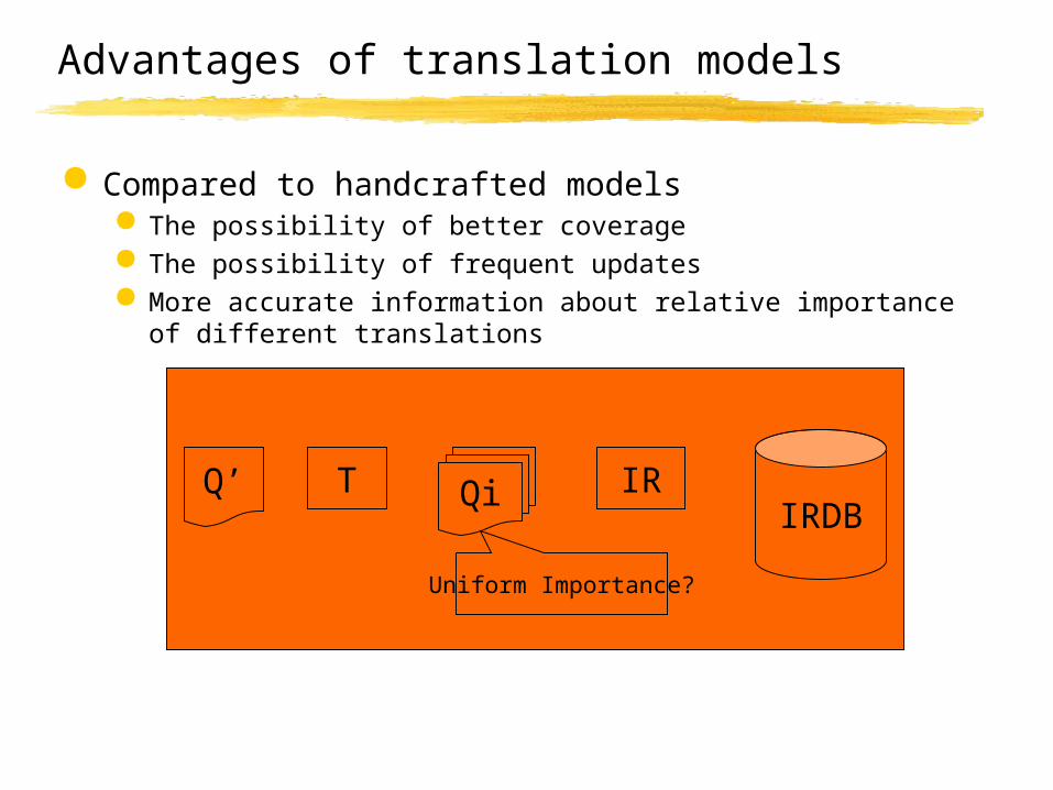
Method A: Competitive Linking
Step 1: Co-occurrence counts
Use “whole” table information Initialize score(u,v) to G2(u,v) (similar to Chi-square)
Good-Turing Smoothing gives improvements
u !u Total
v cooc(u,v) cooc(!u,v) cooc(.,v)
!v cooc(u,!v) cooc(!u,!v) cooc(.,!v)
Total cooc(u,.) cooc(!u,.) cooc(.,.)

Step 2: Estimation of link counts
Competitive Linking algorithm is employed
Greedy approximation of the MAP approximation
Algorithm1. Sort all score(u,v) from the highest to the lowest2. For each score(u,v) in order:
Link all co-occurring token pairs (u,v) in the bitext(If u is NULL consider all tokens of v in the bitext linked to NULL and vice versa)
One-to-One assumption: Linked words cannot be linked againRemove all linked words from the bitext
Example: Competitive Linking
ba
c d
u
v

Competitive Linking
X X XX
XX
X X
XX
XX
Xu
v
ba
c d

Competitive Linking
X XXX X X
X
XX
X XX
XX
X XX X
XX X
XXX
u
v
ba
c d

Competitve Linking per sentence
b a… …
c d… …
a b… …
c d e… …
links(a,c)++links(b,d)++…
links(a,d)++links(b,e)++…

Building Lexicons
Introduction Previous Work Translation Model Decomposition Reestimated Models Parameter Estimation Method A Method B Method C Evaluation Conclusion

Method B:
“Most texts are not translated word-for-word”
Why is that a problem with Method A?
a b x… …
c d e f… …

Method B:
“Most texts are not translated word-for-word”
Why is that a problem with Method A?
a b x… …
c d e f… …
a b x… …
c d e f… …
We are forced to connect (b,d)!
Competitive Linking

Method B:
After one iteration of Method A on 300k sentences Hansard
links = coocoften, probably
correct
links < coocrare, might be
correct
links << coocoften, probably
incorrect

Method B:
Use information links(u,v)/cooc(u,v) to bias parameter estimation
Introduce p(u,v) as the probability of u and v being linked when they co-occur.
Leads to binomial process for each co-occurrence (either linked or not linked)
Too sparse data to model p(u,v) Just 2 cases:
),( vup If u,v are mutual translations(Rate of true positives)
If u,v are not mutual translations(Rate of false positives)
),( vup

Method B
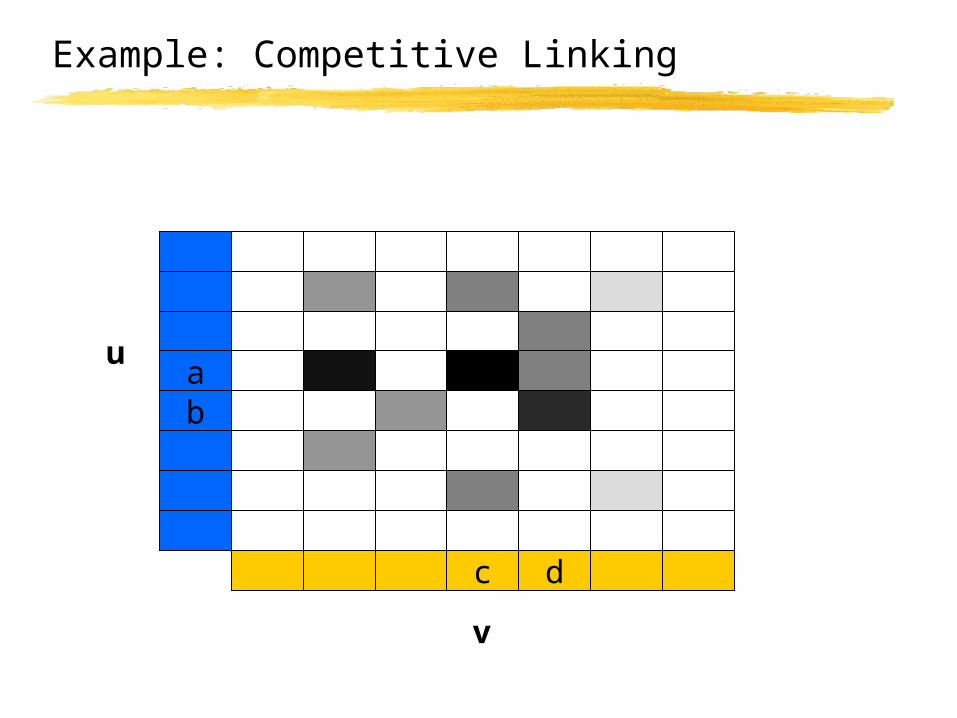
Maximum Likelihood Estimation

Maximum Likelihood Estimation
on 300k sentences Hansard

Method B:
Overall score calculation for Method B:
Probability for generating correct links(u,v) given cooc(u,v):
Probability for generating incorrect links(u,v) given cooc(u,v):
Score is ratio
)),,(|),(( vucoocvulinksB
)),,(|),((
)),,(|),((log),(
vucoocvulinksB
vucoocvulinksBvuscoreB
)),,(|),(( vucoocvulinksB

Building Lexicons
Introduction Previous Work Translation Model Decomposition Reestimated Models Parameter Estimation Method A Method B Method C Evaluation Conclusion

Method C:
Improved Estimation using Preexisting Word Classes
Method A, B: All word pairs that co-occur the same number of times
and are linked the same number of times are assigned the same score
But: Frequent words are translated less consistently than rare words
Introduce classes to get Statistics per class
)),,(|),((
)),,(|),((log)),(|,(
Z
ZC vucoocvulinksB
vucoocvulinksBvuclassZvuscore

Building Lexicons
Introduction Previous Work Translation Model Decomposition Reestimated Models Parameter Estimation Method A Method B Method C Evaluation Conclusion

Method C for Evaluation
We have to choose classes: EOS: End of sentence punctuation EOP: End of phrase punctuation (, ;) SCM: Subordinate clause markers (“ () SYM: Symbols (~ *) NU: NULL word C: Content words F: Function words

Experiment 1:
Training Data 29,614 sentence pairs French, English (Bible)
Test Data 250 hand linked sentences (gold standard)
Procedure Single Best: Models guess one translation per word on
each side Whole Distribution: Model outputs all possible
translation with probabilities

Experiment 1 – Results
Single Best – All links (95% confidence intervals)
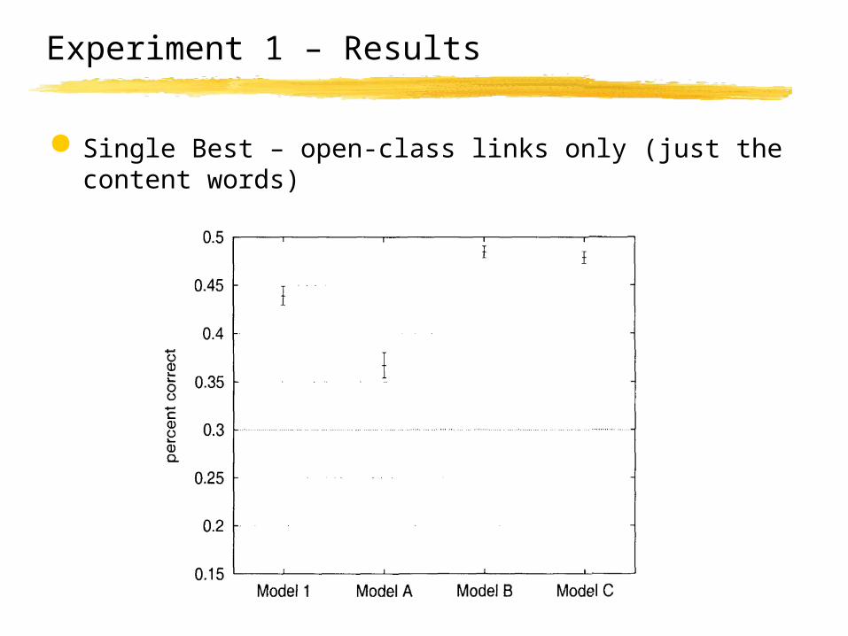
Experiment 1 – Results
Single Best – open-class links only (just the content words)
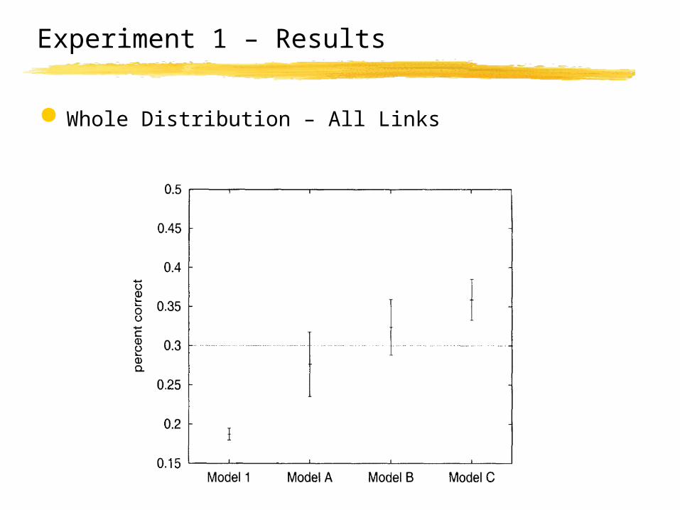
Experiment 1 – Results
Whole Distribution – All Links

Experiment 1 – Results
Whole Distribution – open-class links only (just the content words)

Experiment 2:
Influence of training data size
Model A is 102% more correct than Model 1 when trained on only 250 sentence pairs
Overall up to 125% improvements

Evaluation at the Link Type Level
Sorted scores for all link types:
1/1, 2/2 and 3/3 correspond to links/cooc

incomplete: Lexicon contains only part of correct phrase
Coverage vs. Accuracy

Building Lexicons
Introduction Previous Work Translation Model Decomposition Reestimated Models Parameter Estimation Method A Method B Method C Evaluation Conclusion

Conclusion - Overview
IBM Model 1: co-occurrence information only
Method A: one-to-one assumption
Method B: Noise Model
Method C: condition auxiliary parameters on word classes
a b x… …
c d e f… …
a b x… …
c d e f… …
a b x… …
c d e f… …