Budget Constraint: Review Consumers cannot afford all the goods and services they desire. Consumers are limited by their income and the prices of goods. Model Assumption: Consumers spend all their income (no savings). Let: M=Income X and Y are two goods Px=price of each unit of good X Py = price of each unit of good Y Budget constraint: numerical expression of which market baskets the consumer can afford. The Budget Constraint: PxX + PyY = M Total expenditure = Income Rearranging the above expression for the budget constraint, we are able to determine how many units of good Y we can consume for any given quantity of good X:

Y M

PPP

XY

X

Y

= −

This equation of a straight line illustrates the trade-off between Y and X.

Y

MPy

X

0 MPx

Dividing income by the price of Y yields the maximum number of units of Y that can be purchased when no units of X are purchased. Dividing income by the price of X yields the maximum number of units of X that can be purchased, when no units of Y are purchased. These are the intercepts of the budget line.

The slope of the equation −

PP

X

Y is negative because in order to

purchase more units of Y, the consumer must give up units of X.

Slope of budget constraint is −PP

x

y

.

Shifts in the Budget Constraint What happens to the budget constraint when: (1) income changes, (2) the price of X changes or (3) the price of Y changes? 1) Income changes Let M0= initial income M1=new income When income changes the Y intercept changes from M

PY

0

to MPY

1

and

the X intercept changes from IPX

0

to IPX

1

.

The slope of the budget line remains unchanged at − PP

X

Y.

Hence, a change in income is shown as a parallel shift inward or outward of the budget constraint. # Units of Y

MPY

1

MPY

0

#Units of X

0 MPx

0

MPx

1

BL1BL0

Budget line after an increase in income.

(2) A change in the price of good X: A change in the price of good X does not change the amount of good Y the consumer could buy if he or she spent all their income on Y. (i.e. the intercept remains the same.) The budget line does change: For price increases, the budget line becomes steeper For price decreases, the budget line becomes flatter. # Units of Y

MPY

1

#Units of X 0 M

Px0

MPx

1

Let PX

0 = the initial price of good X. Let PX

1 = the new (lower) price of X. When the price of X decreases, the consumer can now purchase more of good X. The budget constraint swings outward and becomes flatter.

BL1BL0

Budget line after a decrease in the price of X.

(3) A Change in the Price of Good Y: A change in the price of good Y does not change the amount of X the consumer could buy if he or she spent all their income on X. (I.e. the X intercept remains the same.) However, the budget line does change: For price increases the budget constraint becomes flatter.

For price decreases the budget constraint becomes steeper. (I.e. the Y intercept increases.)

# Units of Y

MPy

1

MPy

0

#Units of X 0 M

Px0

Let PY0

= the initial price of good Y.

Let PY1

=the new (lower) price of Y. Note: If all prices and income change by the same proportion, the budget constraint is unaffected.

BL1

BL0

Budget line after a decrease in the price of Y.

1

Consumer Choice

Constraints:

PricesIncome

(Endowments)

• BudgetConstraint

• Time Constraint

Preferences:

Represented by:

IndifferencesCurves

Utility Functions

Optimal Choice:

Maximize Utilitys.t. constraints

• Demand for Goods• Labor Supply

• Savings

2

Budget Constraint:

Imagine: You have $24 (Y=24) to spend on beer (x1) and pizza (x2). Beer costs $2 per cup(p1 = 2) and pizza costs $3 per slice (p2 = 3).

The budget constraint is:2x1 + 3 x2 = 24 => x2 = 8 - 2

3 x1

or, in general :p1x1 + p2 x2 = Y => x2 =

2

Yp - 1

2

pp x1

Assume :• Can consume fractions of beer, pizza• Can’t consume negative beer or pizza

(Note: can have, in principle, any # of goods

p1x1 + p2x2 + p3x3 + p4x4 + . . . + pNxN = Y

Also, we can aggregate several good together to compare x1 with “all other goods” x2 )

3

2x1 + 3 x2 = 24 => x2 = 8 - 23 x1

p1x1 + p2 x2 = Y => x2 =2

Yp - 1

2

pp x1

Slope of the budget line is the “opportunity cost”:number of slices of pizza need to give up to consume one more cup of beer.

1

Yp =12

x1 : Cups of Beer

x2 :SlicesOfPizza

2

Yp = 8 Slope = 1

2

23

pp

− = −

4

• Budget Constraint (Budget Set, Affordable Set, Feasible Set): Triangle and Interior

• Budget Line : Just the line:

2x1 + 3 x2 = 24

On Budget Line: spend all moneyInside the Budget Line: have money left over.

E.g.: Consider these bundles (baskets):

(x1, x2) = (0, 8) (12, 0)

(3, 6) (5, 4.67)

are all on the budget line.

(x1, x2) = (0, 7) (0, 0)

(3, 5) (5, 4.2)

are all affordable (feasible), but not on the budget line.

(x1, x2) = (0, 9) (12, 12)

(3, 6.5) are not affordable (not feasible).

5

Shifts in the Budget Constraint (income):

Suppose Y increases to $30:2x1 + 3 x2 = 30 => x2 = 10 - 2

3 x1

Change in income: parallel shift in budget lineIncrease (decrease in income): shift out (in)

12 15x1 : Cups of Beer

x2 :SlicesOfPizza

10

8 Slope = - 23

6

Shifts in the Budget Constraint (price)

Suppose p1 increases to $4:4x1 + 3 x2 = 24 => x2 = 8 - 4

3 x1

Change in a price: change in slope of the line.Price increases: budget set smaller.

Q: What if all prices, and income triple?

12x1 : Cups of Beer

x2 :SlicesOfPizza

8 Slope = - 43

6

7

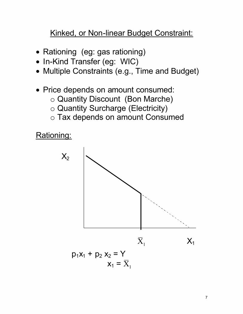
Kinked, or Non-linear Budget Constraint:

• Rationing (eg: gas rationing)• In-Kind Transfer (eg: WIC)• Multiple Constraints (e.g., Time and Budget)

• Price depends on amount consumed:o Quantity Discount (Bon Marche)o Quantity Surcharge (Electricity)o Tax depends on amount Consumed

Rationing:

p1x1 + p2 x2 = Yx1 = 1X

1X X1

X2

8

In-Kind Transfer:

E.g.: Kid has $30 to spend this week on healthylunches and soda (pop). Healthy lunches cost$6 each, and soda costs $3 per gallon.

Two options: Give $30 more in cashGive 5 healthy lunches

What if he can sell lunches for $6 each? $3?What are other examples of in-kind transfers?Why do we use them instead of cash?

20Soda(x2)

10

5 10 Lunches (x1)

Original Budget Constraint :6x1 + 3x2 = 30

With Cash Value :6x1 + 3x2 = 60

9

Quantity Discount:

E.g. Fertilizer is $5 per pound.o If Buy more than 20 pounds, price is $4

Question: Does the discount apply: (1) to just the fertilizer over the 20 pounds(2) to all the fertilizer

Suppose you have $200 to spend on fertilizer,and all other goods. Let the price of all other goods (p2) be $1.

10

Case 1: Discount only on incremental units

What is the budget line if no kink?5x1 + x2 = 200

Where is the kink (i.e., at what point does the slope change?)

x1 = 20 => x2 = 100

What is the price beyond the kink?p’1 = 4

What is the maximum number of pounds?x1(max) = 45

x2200

100

20 40 45 x1

Slope = -5

Slope = -4

11

Case 2: Discount on all units

What is the budget line if no kink?5x1 + x2 = 200

Where is the kink (i.e., at what point does the slope change?)

x1 = 20 => x2 = 100

What is the price beyond the kink?p’1 = 4

What is the maximum number of pounds?x1(max) = 200/4 = 50

20 40 50 x1

Slope = -5

Slope = -4

12

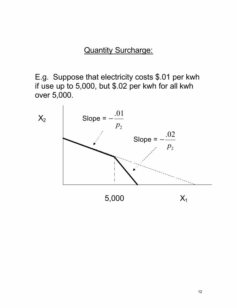
Quantity Surcharge:

E.g. Suppose that electricity costs $.01 per kwh if use up to 5,000, but $.02 per kwh for all kwh over 5,000.

5,000 X1

X2 Slope = 2

.01p

−

Slope = 2

.02p

−

13

Time and Budget Constraints

E.g.: Joel has $40 to spend this weekend on movies (x1) and meals (x2). Movies cost $8 each and meals cost $10 each. So, his budget constraint is:

8x1 + 10x2 = 40

Also, he has only 9 free hours. Movies take 3 hours each, and meals take 1 hour. So, his time constraint is:

3x1 + 1x2 = 9

3 5 X1

X2

9

4

Time Constraint: Slope = -3

Budget Constraint:Slope = -4/5

Topic 4 page42

Taxes, Trade Limitations and Market Restriction On Total Surplus Total Surplus = consumer surplus + producer surplus

A Per Unit Tax on A Competitive Firm When a per unit tax is imposed on the firm, the firm’s profit function becomes: Total profit = total revenue - total long-run cost - total taxes

π ( ) ( )q Pq C q tL= q− − where tq are total taxes paid by the firm to the government. (t=tax; q= quantity produced) In order for the firm to maximize profits, it must produce an output such that it must satisfy:

P C q

qtL= +

ΔΔ

( )

The firm considers the per unit tax a cost of doing business. It determines output where price equals the sum of long run MC and t.

Topic 4 page43

Price MCL ACL +tax ACL tax Pm 0 q Quantity

MCL+tax

Pm +tax

For the firm, when it considers the tax as another cost, the long run average cost of the firm becomes ACL + tax. The curve is exactly the same as the pre tax LAC curve, only shifted up by the amount of the per unit tax. The MC function also shifts up by the amount of the tax and becomes MCL + tax. Since the average and marginal cost functions shift upward by the amount of the ‘tax’, the new and old long-run average cost functions reach a minimum at the same quantity produced. Both long run average cost curves reach a minimum at q.

Topic 4 page44

Price SL +tax B SL tax P0 A Demand 0 Q1 Q0 Quantity

P0 +tax

The green box represents the total amount of tax revenue collected by the government. For the industry, the long-run equilibrium price increases from P0 to P0+tax. The equilibrium quantity produced decreases from Q0 to Q1. By raising the per unit tax, the government increases the price of the product and decreases the quantity demanded. Before tax, industry output at point A at price P0.

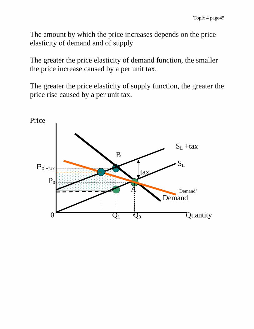
Topic 4 page45

The amount by which the price increases depends on the price elasticity of demand and of supply. The greater the price elasticity of demand function, the smaller the price increase caused by a per unit tax. The greater the price elasticity of supply function, the greater the price rise caused by a per unit tax. Price SL +tax B SL tax P0 A Demand’ Demand 0 Q1 Q0 Quantity

P0 +tax

Topic 4 page46

The Effect of A Per Unit Tax on Consumer and Producer Surplus It has been shown that the behaviour of consumers and producers change when a tax is imposed. Taxes have social consequences. Price CS Supply

P0

PS Demand 0 Q0 Quantity

Before the government imposes a per unit tax, the long-run equilibrium price and quantity in a competitive industry are P0 and Q0. Consumers benefit because they are willing to pay more than P0 for each unit up to the Q0

th . The area between the demand curve and the price measures consumer surplus. Producers receive P0 for all the units they sell, even though they are willing to supply all units up to the Q0

th unit at lower prices. The area between the price line P0 and the industry supply function represents producer surplus when producers sell Q0 units are price P0.

Topic 4 page47

Now impose the Per Unit Tax: The sum of consumer and producer surpluses decreases when the government imposes a per unit tax on a competitive industry. Price Supply + tax CS A Supply P1

B D P0

C P2

Demand P3 0 Q1 Q0 Quantity The market price increases to P1 and equilibrium quantity decreases to Q1 when the tax is imposed. Consumer surplus decreases by area P0 P1 AD. Consumer surplus is now P1 P4 A. Producer surplus in now area P3 P2C. Although producers receive P1 for Q1 units, they must pay the government the tax of area P2P1 AC. Producer surplus has decreased by area P2P0 DC. Dead weight loss= ADC (loss of consumer and producer surplus that is not offset by an increase in value to some other group.

Utility Maximization Under Constraint 2 Methods

Question: Tom spends all his $100 weekly income on two goods, X and Y. His utility function is given by U(X, Y) = XY. If Px= $4/ unit and Py=$10/ unit, how much of each good should he buy to maximize utility?

The budget constraint equals:

P X P Y MX Yx y+ =

+ =4 10 100

Method 1: Lagrangean Multipliers: First, transform the constrained maximization problem into the following unconstrained maximization problem:

Max U X Y P X P Y MX Y x y, ,

L ( , ) ( )λ

λ= − + −

The lagrangean multiplier’s (λ ) role is to assure that the budget constraint is satisfied.

The first order conditions for a maximum of L are obtained by taking the first partial derivatives of L with respect to X, Y and λ , and equating them to zero:

Max XY X Y

XY

YX

X Y

X Y, ,L ( )

(

λλ

∂∂

λ

∂∂

λ

∂∂λ

= − + −

= − =

= − =

= − + − =

4 10 100

4 0

10 0

1 4 10 100 0

L

L

L

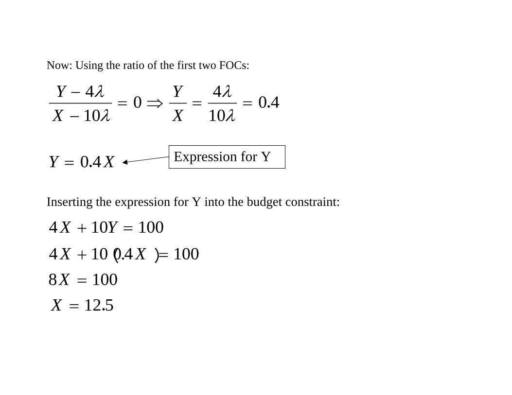
Now: Using the ratio of the first two FOCs:

YX

YX

Y X

−−

= ⇒ = =

=

410

0 410

0 4

0 4

λλ

λλ

.

.

Inserting the expression for Y into the budget constraint:

4 10 1004 10 0 4 1008 100

12 5

X YX . XX

X

+ =

+ ===

︵ ︶

.

Expression for Y

Substituting X=12.5 into the expression for Y:

Y X

Y

=

= =

0 4

0 4 12 5 5

.

. ( . )

The bundle X=12.5 and Y=5 will maximize utility while constrained at M=100.

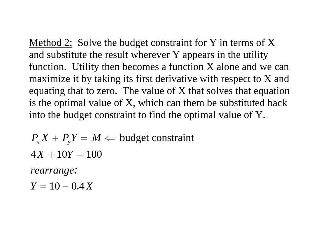
Method 2: Solve the budget constraint for Y in terms of X and substitute the result wherever Y appears in the utility function. Utility then becomes a function X alone and we can maximize it by taking its first derivative with respect to X and equating that to zero. The value of X that solves that equation is the optimal value of X, which can them be substituted back into the budget constraint to find the optimal value of Y.

P X P Y MX Y

rearrangeY X

x y+ = ⇐

+ =

= −

budget constraint4 10 100

10 0 4:.

The utility function: U X Y XY

U X Y X X X X

Max Utility wrt XUX

X

X

( , )

( , ) ( . ) .

:

.

.

=

= − = −

= − =

=

10 0 4 10 0 4

10 0 8 0

10 0 8

2

∂∂

X = 12.5Y = 10 - 0.4X = 10 - 0.4(12.5) = 5

Same answer: (X=12.5, Y=5)

Graphically:

Y 10 5 U=62.5 0 12.5 25 X Which leads us to indifference curves:

Budget line