THE INTERTEMPORAL GOVERNMENT BUDGET CONSTRAINT AND TESTS FOR

BUBBLES

Graham Elliott

Reserve Bank of Australia

Colm Kearney

University of New South Wales

Research Discussion Paper 8809

November 1988

Research Department Reserve Bank of Australia

We would like to thank Warwick McKibbin, Dirk Morris, Malcolm Edey, Rob Trevor and participants at the 16th Autralian Conference of Economists for helpful discussions. The views expressed are those of the authors and should not be interpreted as views of the Reserve Bank of Australia.

ABSTRACT

The methodology for the testing of bubbles in asset prices has recently been applied to testing the sustainability of government debt accumulation. In particular, Hamilton and Flavin (1986) and MacDonald and Speight (1987) use the methodology developed by Flood and Garber (1980) in an attempt to identify a period of bubble financing of the budget deficit for the US and UK respectively. MacDonald and Speight and Trehan and Walsh (1988) also use recently developed cointegration methods in an alternative test of the hypothesis of unsustainable financing.

This paper uses the above methods to test for bubble financing of the fiscal deficit for Australia. We develop the method to allow for the effects of income growth on the sustainability of deficits and critically appraise some of the methods used in previous studies and suggest improvements. Our finding is that over the period 1953/54 to 1986/87 there is no evidence of unsustainabiltiy of government debt. The analysis suggests that instead, seignorage was used to pay for sustained fiscal deficits, and that the overall level of debt as a ratio of GDP fell over the period as a result of strong GDP growth and inflation.

(i)

TABLE OF CONTENTS

Abstract

Table of Contents

1. Introduction

2. The Intertemporal Government Budget Constraint

3. Testing for Bubble Financing

4. Empirical Evidence

(a) The Cointegration Test

(b) The Restricted Flood Garber Test

5. Conclusion

6. Appendix 1: Data Sources

7. References

8. Figures and Tables

( ii)

i

ii

1

3

8

16

16

19

21

22

23

25

THE INTERTEMPORAL GOVERNMENT BUDGET CONSTRAINT AND TESTS FOR

BUBBLES

1. Introduction

Graham Elliott

Colm Kearney

Much attention has recently been focussed upon the appropriate stance

of fiscal policy. Many macroeconomic analysts and policy makers,

both in Australia and overseas, have argued that protracted fiscal

deficits do not aid economic performance and might adversely affect

future real economic activity by crowding out private investment

expenditures and generating inflation. In addition, concern has

recently been expressed about the sustainability of trends in the

growth of public debt and this has led some governments to embark

upon programmes of fiscal restraint in order to reduce their levels

of outstanding debt. As Blanchard, Dornbusch and Buiter (1986) point

out, an interesting question in this regard concerns the optimal path

of debt stabilisation because it is far from clear that the optimal

policy involves the fastest possible adjustment.

The purpose of this paper is to examine the appropriateness of

fiscal stance in relation to the government's intertemporal budget

constraint. The latter relates the sustainable growth of government

debt to the non-interest fiscal deficit, the growth of nominal output

and the service costs of outstanding debt. Specifically, the

government's intertemporal budget constraint provides the sustainable

2

limits to the growth of government debt given the performance of the

macroeconomy. Although this constraint must hold in the long run,

there is ample scope for governments to exceed it over short periods

of time by engaging in so-called bubble financing. Tests for the

existence of bubble financing have been reported by Hamilton and

Flavin (1986), Hakkio and Rush (1987) and Trehan and Walsh (1988) for

the US and by MacDonald and Speight (1987) for the UK. On close

examination, however, a number of problems exist with the method in

some of these studies and this paper presents the corrected tests.

We have developed the framework to allow for the effects of income

growth on debt sustainability and applied the tests to Australian

data over the period 1953/54 to 1986/87. Amongst the main findings

are the lack of evidence of bubble financing in Australia together

with an indication of the historical ~ortance of monetisation for

the financing of non-interest fiscal deficits.

Section 2 presents the framework of the government's intertemporal

budget constraint and explains how it constrains the sustainable

growth of debt. Section 3 generalises the tests of bubble financing

utilising the cointegration methodology of Engle and Granger (1987)

and the approach of Hamilton and Flavin (1986) to allow for income

growth. The tests are applied to the data in Section 4. The final

section summarises the paper and draws conclusions.

3

2. The Intertemporal Government Budget Constraint

In order to examine the relationship which exists between the

government's fiscal stance and the performance of the macroeconomy,

the appropriate framework is the government's intertemporal budget

constraint. This can be written either in nominal terms and\or as a

proportion of GDP and it establishes the link which exists between

the prevailing level of government indebtedness and the future debt

servicing requirements.

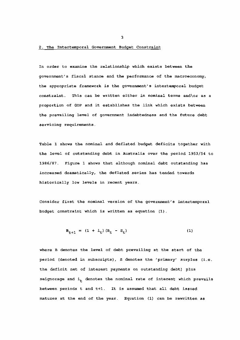
Table 1 shows the nominal and deflated budget deficits together with

the level of outstanding debt in Australia over the period 1953/54 to

1986/87. Figure 1 shows that although nominal debt outstanding has

increased dramatically, the deflated series has tended towards

historically low levels in recent years.

Consider first the nominal version of the government's intertemporal

budget constraint which is written as equation (1) .

(1)

where B denotes the level of debt prevailing at the start of the

period (denoted in subscripts), S denotes the 'primary' surplus (i.e.

the deficit net of interest payments on outstanding debt) plus

seignorage and it denotes the nominal rate of interest which prevails

between periods t and t+1. It is assumed that all debt issued

matures at the end of the year. Equation (1) can be rewritten as

4

= ( 1) I

If we start at time t=O and solve equation (1)' recursively forward

in time, we obtain equation (2)

= +

which yields the intertemporal budget constraint by utilising the

transversality condition that the level of outstanding nominal debt

does not permanently grow at a faster rate than the nominal interest

rate, i.e.,

lim t~oo

(3)

By imposing this transversality condition (3) in equation (2) and

denoting the nominal discount factor by Rt = 1/ (l+i0 ) ... (l+it), we

can simplify the nominal version of the government's intertemporal

budget constraint to equation (2)'

= (2) I

which states simply that the present value of debt servicing

obligations must be equal to the prevailing level of outstanding

debt.

5

It is pertinent to note that the public sector borrowing requirement

constitutes an inappropriate indicator of the government's fiscal

stance. The inclusion of public trading enterprises in the measure

of the deficit is misleading as these corporations resemble and act

as private enterprises. From the perspective of the budget

constraint, only the subsidies paid to and receipts received from

these enterprises are relevant. Accordingly, the Australian

government's fiscal deficit measure which is employed in

this paper is obtained by aggregating the Commonwealth and State and

Local authorities' revenues and outlays net of public trading

enterprises.

As Blanchard, Dornbusch and Buiter (1986) point out it is

illuminating to express the government's intertemporal budget

constraint as a proportion of GDP. By noting that the growth rate of

nominal output (Yt+l-Yt)/Yt is equal to the sum of real output growth

(yt) plus inflation (pt),

= (4)

and we use this to deflate the nominal budget constraint of equation

(1)' to get

= + (5)

6

Proceeding as before, the real version of equation (2)' is equal to

where;

=

8 t = t

This expression can be simplified to (6)' by writing

( 6)

8 = (l+y) (l+p)/(l+i) where y,p and i denote respectively the long

te~ average growth of real output, the long te~ average inflation

rate and the long te~ interest rate (the analysis henceforth uses

these long te~ averages with the bar dropped from equations);

= ( 6) '

The interesting aspect of this version of the government's

intertemporal budget constraint is that it demonstrates how higher

growth of nominal output (i.e. either higher real output growth

and/or higher inflation) reduces the burden of debt repayments. As

long as the long te~ average growth in nominal output exceeds the

long te~ average nominal interest rate, the government is not

constrained by the amount of debt it can service. Because this is

not generally the case, however, governments are faced with a

constraint which will be binding if the growth of debt equals

(l+i)/(l+y) (l+p) which implies that on average new issues of bonds

are restricted in their amount to cover interest payments on the

current level of outstanding debt.

7

It is generally the case in real economic circumstances that the

rate of growth of government bonds diverges from the upper limit

implied by the intertemporal budget constraint. There is not

necessarily a mechanism to prevent governments from issuing debt in

such quantities that its future growth exceeds the sustainable rate

which is implied by nominal output growth and nominal interest rates,

at least over a short period of time. If this occurs, the government

is said to be engaging in bubble financing of it's fiscal deficit.

There is an adjustment mechanism, however, which causes the

constraint to apply over time. When government debt is imperfectly

substitutable for other private sector financial assets, the price of

bonds must fall in order to induce portfolio balancers to take up the

debt. The resulting higher debt servicing costs are also reflective

of the increased incentive which is required to offset investors'

uncertainty about whether the government will be able to honour it's

future debt obligations.

8

3. Testing For Bubble Financing

In this section, we examine two tests for the existence of bubble

financing in Australia ove~ the period 1953/54 to 1986/87. The first

test employs the cointegration method pioneered by Granger (1981) and

Engle and Granger (1987) which has been utilised by MacDonald and

Speight (1987) to examine the British case and Hakkio and Rush (1987)

and Trehan and Walsh (1988) for the US. The second test investigates

the price level bubble approach pioneered by Flood and Garber (1980)

and adapted to examine the intertemporal government budget constraint

for the US by Hamilton and Flavin (1986) .

Cointegration can be defined as follows. If the components of a

vector xt have a stationary invertible ARMA representation after

differencing d times, then xt is said to be integrated of order d,

i . e . xt - I (d) . Variables integrated of the same order are said to

be cointegrated of order d,b, if there exists a linear combination of

these variables such that Zt = a'xnt is integrated of order d-b where

d,b>O. In the special case where d=b, Zt is stationary. This

implies that the general trend in each series is the same; there is a

common path followed by the two series which, although it may not

hold at all points, is returned to time and time again.

The first of these tests is derived from equation (1) .

rearranged to give the following equation:

(l+i)/(l+y) (l+p)bt-1

This can be

(7)

9

where the lower case letters g,t,m, and b refer respectively to the

government spending, taxation, the money base and debt outstanding

deflated by GDP. Seignorage (financing the deficit by expansion of

the money base) 1 is included as the government can simply issue money

to pay its bills.

When the constraint is binding, the change in the level of bonds must

be stationary. This is proved formally for the nominal case in

Trehan and Walsh (1988) 2 . The point is seen by rearranging equation

(7) in the form

~t = gt - (tt + ~t> + ((l+i)/(l+y) (l+p) - l)bt-1 (7)'

which is approximately (and exactly in continuous time) equal to

(7) ,,

The last term here is s~ply the interest payments on debt deflated

by GDP growth and inflation. For debt not to be explosive the right

hand side of the above equation must be stationary (it may have a

negative deterministic component over a sample if debt is being

repaid) . This differs from the related equation in Trehan and Walsh

(1988) as it allows for the possibility that inflation and/or

1 In this paper seignorage refers to financing the deficit by issuing money (inflation tax is treated separately) . Even though the government may issue enough debt to finance a deficit, if this debt is taken up by the central bank then the effect is as if the central bank printed the money.

2 The proof is lengthy and will not be reproduced here.

10

economic growth may finance the deficit. Trehan and Walsh (1988)

point out that the requirement that the deficit excluding interest

payments be stationary for sustainability (as tested in Hakkio and

Rush (1987) and MacDonald and Speight (1987)) is not sufficient; the

deficit including interest rates must be stationary.

There is a special case when these two hypotheses will be identical.

If the deficit excluding interest rates is stationary (as in the null

hypothesis of Hakkio and Rush (1987)) equation (7)'' reduces to

~b = t (i-y-p)bt_1 + a stationary term (8)

The change in the bond series will be stationary if y+p is greater

than i. This corresponds to a root of the bond series of 1+i-y-p

which is less than one. The bond series and thus the deficit

including as well as excluding the deficit is stationary. This shows

that the tests for a deficit including and excluding interest

payments are equivalent in this case.

In general, however, the right hand side of equation (7)'' will be

stationary if the sum of the trends in each of the variables cancel.

This allows for the possibility that the deficit excluding interest

payments to be non stationary and still satisfy the constraint if it

is cointegrated with interest payments.

One test of the above hypothesis is to test the right hand side of

equation (7)' for stationarity. This is equivalent to imposing a

11

cointegrating relationship (with a cointegrating vector of (1 -1 -1))

between the government spending (inclusive of interest), taxation and

seignorage variables.

Previous researchers have variously tested for cointegration between

the variables including and excluding interest payments. Trehan and

Walsh (1988) employ U.S. data to test both the restricted model and

the unrestricted model when interest payments are included in the

deficit. In each case they accept the hypothesis of a stationary

deficit although in the unconstrained estimation the coefficient for

their seignorage variable is not close to unity3 . Hakkio and Rush

(1987) and MacDonald and Speight (1987) both test the unrestricted

model employing the deficit excluding interest payments for U.S. and

U.K. data respectively. Both accept the hypothesis of cointegration

with coefficients close to unity. From the argument from Trehan and

Walsh (1988) regarding inclusion of interest rates, and our argument

relating the two hypotheses under the special condition of income

growth and inflation outpacing interest rates, the two sets of

results are invalid (as they do not allow for income growth the

special condition cannot hold) .

It is important to notice that if the primary deficit is financed by

money creation, it is likely that the hypothesis of cointegration

will be accepted. This is not an unlikely finding for Australia as

it is only recently that the government has been able to determine

3 The likely cause of this is that their seignorage variable is stationary. Their test for non stationarity accepts at the 10% level of significance. However, further tests using this variable show that its addition to a stationary variable results in a stationary variable. This is a contradiction to the original finding.

12

the amount of debt that it issues. Prior to this, the institutional

arrangements for issuing debt in Australia have involved the

government setting the price while allowing the private sector to

take up as much or as little as desired. That which was not

purchased by the public resulted in increases in the holdings of debt

by the Reserve Bank. Seignorage therefore became the residual

financing instrument of the primary deficit in Australia over the

sample period analysed in this paper. Figure 2 illustrates this

point. Both the gt (excluding interest payments) and (tt+~t) series

follow very similar paths.

The second test is based upon Hamilton and Flavin's (1986) adaptation

of Flood and Garber's (1980) test for hyper-inflationary bubbles to

examine whether governments have resorted to bubble financing of

their fiscal deficits. The test is derived from equation (2) above

and reproduced below as equation (9) .

= + BN(l+y)N(l+p)N(l+i)N

. (l+i)t/(l+y)t(l+p)t

This specification shows us that the level of debt outstanding at

time t is equal to the sum of all future surpluses plus the present

value of debt outstanding at time t=N. Taking expectations of the

(9)

right hand side of this equation; the current level of debt is equal

to agents expectations of future surpluses and their expectation of

the amount of debt that will not be repatriated. In particular if

lim N~~

= 0 (10)

13

the present value of bonds held at time N is zero and the constraint

holds. This does not preclude a positive holding of bonds in the

limit (i.e BN need not tend to zero as long as its present value

does) which means that the government can continue to roll over debt

so long as the debt is not increasing at a rate greater than

(l+i) I (l+y) (l+p) . The test is based on the existence of this teDm.

If the limit of this is zero the teDm drops out of the equation (9)

while if it is not, the bubble teDm will remain. Hamilton and Flavin

(1986) show that if the limit approaches a constant then the

alternative hypothesis is that

N

= s. ~

+

with a significant value for A0 indicating that investors do not

expect that the government will be able in the limit to repatriate

all its outstanding debt.

( 9) ,

It can be seen that the first teDm in equation (9)' cannot be tested

because we cannot measure the expected future path of the government

surplus, both Hamilton and Flavin (1986) and MacDonald and Speight

(1987) assume that current trends in the surplus will continue into

the future. Whilst this does not constitute the full infoDmation set

which investors consider in making expectations of future surpluses,

this extrapolation is consistent with our test insofar as we are

testing the hypothesis that current trends in government spending and

financing decisions ~ply that the level of debt is too high. The

expected surplus teDm can therefore appropriately be proxied in the

14

present context by utilising an autoregressive representation of past

surpluses. The expectations ter.m was substituted out in the method

of Hansen and Sargent (1981) . For a lag length of one4

= +

This equation is estimated jointly with the autoregression of st

+

The bubble ter.m in equation (11) is:

where A0 is the coefficient to be estimated and t is a time trend.

Considering the variable (1/8t) where 8 is constant, the variable is

a deter.ministic ter.m integrated of order greater than one. The

(11)

(12)

intuition of this result is that for (l+i) > (l+y) (l+p), (which must be

the case if there is a constraint as in Hamilton and Flavin (1986)),

then this ter.m trends upwards over time. This ter.m will pick up any

deter.ministic trend in the bond series which is not accounted for by

the surplus (including seignorage) . The bond series in Hamilton and

Flavin (1986) is stationary, which precludes the finding of a

significant coefficient on the bubble ter.m.

4 Initially three lags were specified. Use of likelihood ratio tests for the full system resulted in acceptance of a lag length of one.

15

If i<y+p, the bubble te~ asymptotes to zero (the specification no

longer tests for a bubble) . The limit te~ can approach any value as

1/ot goes to zero as t increases. Thus a finding of a significant A0

here is compatible with the hypothesis that the constraint is

holding.

Once non-stationarity of the bond series is established, we can no

longer make use of the usually applied t-statistic on the bubble te~

as it is no longer t distributed (Durlauf and Phillips (1986)), a

point which is overlooked by Macdonald and Speight (1986) 5 . An

alternative to testing by the above method is necessary to dete~ne

whether or not the bubble te~ is correctly included in the model.

Hall (1986) examines the inclusion of a variable in a cointegrating

equation on the strength that its inclusion is necessary for white

noise residuals to be obtained. Thus the method of testing is to

test the restricted equation's residuals for stationarity (i.e. no

bubble te~) . If the residuals remain stationary when the te~ is

excluded then it is not significant. This can be applied by noting

that when the series for bonds is integrated at a higher order than

the fundamentals, then the residuals of the estimated equation

(excluding the bubble te~) will be non-stationary. If the inclusion

of the bubble te~ results in an equation with stationary residuals

then the bubble te~ is found to be correctly included and

significant.

5 These authors did not report any diagnostic checking of their final system of equations. What is likely is that the price level effects contained in the bond series is appearing in the equation through a significant dete~inistic trend (i.e the bubble te~ is significant) . This may explain why they obtain results in conflict with their (possibly incorrect) cointegration results.

16

4. Empirical Evidenca

A description of the data including sources is included in Appendix

1. For our sample, the average nominal interest rate is exceeded by

the rate of growth of real GDP plus average inflation. This means

that in the first test use of the deficit including and excluding

interest payments are equivalent. Also, in the second test a

significant "bubble term" is not a finding of debt unsustainability

but instead is compatible with the hypothesis that debt is being

repatriated over the period.

a. The Cointegration Test

We apply the cointegration test described in the previous section to

test the hypothesis that government spending (inclusive and exclusive

of interest payments), taxation and monetary policy have been

conducted in such a way that bonds are growing on an unstable path.

It is first necessary to determine that both series are integrated of

an equal order greater than one. An examination of the graphs for the

series under consideration shows that each of the series has trended

upwards with a large jump in the early seventies. This trend in the

data indicates that it is likely that the series are non-stationary.

The results of Dickey-Fuller tests (Dickey and Fuller (1979) and

(1981)), Perron and Phillips (1987) and Stock and Watson (1986) are

given in Table 2 6 . The government spending series (including and

excluding interest payments) and the constructed taxation plus the

6 All results refer to data deflated by GDP.

17

seignorage series appear to be non-stationary around a linear time

trend, i.e., there appears to be both a deter.ministic component and a

stochastic unit root. The deter.ministic components of the series are

not removed as it is the time path of the series we are interested

in, and it is the equivalence of the non-stationary components

between the series (both deter.ministic and stochastic) which is to be

tested. The first differences of all series were tested for non-

stationarity in the same manner as above. All tests reject non­

stationarity indicating that all series under consideration are

integrated of order one.

tests.

We can now proceed with the cointegration

The results for the cointegration test for the equivalence of the

unit roots in the two series are shown on Table 3. The tests for

cointegration are those proposed by Engle and Granger (1987), namely,

their cointegrating regression Durbin Watson test statistic (CRDW)

and the Dickey-Fuller statistic (DF) . Both methods amount to the

testing of the residuals of the cointegrating equation (equation (9))

for non-stationarity, the first uses the method of Bhargarva (1986)

and the second uses the method of Dickey and Fuller. The null

hypothesis of non cointegration of the series is accepted if non-

stationarity of the residuals is accepted. The critical values for

these tests are given in Engle and Yoo (1987) for the case of fifty

observations. It has been shown that tests for non-stationarity such

as these have low power when the alternative hypothesis is that rho

is close to (but less than) one. The test of Stock and Watson (1986)

is also applied. Phillips (1987) and Phillips and Perron (1986) have

proposed non- parametric tests for non-stationarity which have

18

greater power than those considered by Engle and Granger (1987) and

these tests have been applied here.

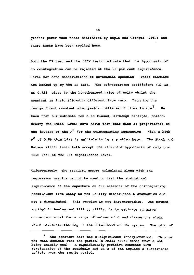
Both the DF test and the CRDW tests indicate that the hypothesis of

no cointegration can be rejected at the 95 per cent significance

level for both constructions of government spending. These findings

are backed up by the PP test. The cointegrating coefficient (a) is,

at 0.934, close to the hypothesised value of unity whilst the

constant is insignificantly different from zero. Dropping the

insignificant constant also yields coefficients close to one7 . We

know that our estimate for a is biased, although Banerjee, Dolado,

Hendry and Smith (1986) have shown that this bias is proportional to

the inverse of the R2 for the cointegrating regression. With a high

R2 of 0.89 this bias is unlikely to be a problem here. The Stock and

Watson (1986) tests both accept the alternate hypothesis of only one

unit root at the 95% significance level.

Unfortunately, the standard errors calculated along with the

regression results cannot be used to test the statistical

significance of the departure of our estimate of the cointegrating

coefficient from unity as the usually constructed t statistics are

not t distributed. This problem is not insurmountable. One method,

applied in Bewley and Elliott (1987), is to estimate an error

correction model for a range of values of a and choose the alpha

which maximises the log of the likelihood of the system. The plot of

7 The constant here has a significant interpretation. This is the mean deficit over the period (a small error comes from a not being exactly one) . A significantly positive constant with stationarity of the residuals and an a of one implies a sustainable deficit over the sample period.

19

the log of likelihoods can be used to calculate critical bounds for

the estimate of a. An alternative method which was foreshadowed in

section III and applied here is to impose the hypothesised value for

a and test the constructed variable for stationarity. If this

variable (i.e. the primary deficit plus seignorage) is stationary,

then we can accept the hypothesised value as a true cointegrating

coefficient.

Tests for the stationarity of the deficit are given in Table 4. It

can be seen that the null hypothesis of non-stationarity is rejected

in both the Dickey Fuller tests and the more powerful Phillips test.

The Stock and Watson (1996) tests indicate that for the series

excluding interest payments stationarity can be rejected at the 99%

level of significance whilst the series including interest payments

rejects the null hypothesis at the 90% level of significance. On this

evidence we accept that government spending and the taxation plus

seignorage variables are cointegrated with a cointegrating

coefficient of unity. As predicted, both specifications of the

deficit (including and excluding interest payments) yield the same

result.

b. The Restricted Flood Garber Test

The bubble test of Hamilton and Flavin (1996) has also been

estimated. As mentioned before, the average nominal interest rate is

exceeded by the rate of growth of real GDP plus average inflation so

the bubble term is not a test for a rational bubble, i.e. a

significant bubble term is compatible with the repatriation of debt

20

over time. The true steady state interest rates should be used here,

but data limitations confine us to the long run average rate over the

sample period of our study.

The results of the estimation of equations (11) and (12) are

presented in Table 5. For lags of the deficit term greater than one,

nonlinear estimation techniques are necessary as there are cross

equation restrictions which are nonlinear. Estimates for more than

one lag of the deficit term show that the extra lags are

insignificant (likelihood ratio tests were employed) . The first

point to note from these tests, given that we expect that the bond

series and the bubble term are non-stationary, is that the equations

should be considered in the framework of the cointegration

literature. The low Durbin Watson coefficient of 0.17 shows that in

fact the bubble term is not fully accounting for the non-stationarity

in the bond series. An analysis of the residuals shows a strong

negative deterministic trend which implies that the negative trend in

the bubble term does not fully explain the determination of the level

of bonds. This could be due to either a mis-specification of the

bubble term or mis-specification of the proxy for expected deficits.

The coefficients given in Table 5 are biased due to both non­

stationarity and the mis-specification; very little trust can be put

into their interpretation. It is interesting to note, however, that

the bubble term is positive in sign. This is further, although very

weak, evidence that inflation tax and GDP growth have contributed

over the period to the sustainability of continuous primary

government deficits.

21

5. Conclusion

The purpose of this paper has been to examine the sustainability of

government debt over the period 1953/54 to 1986/87. To explore this

question, we have used two tests adapted from the literature on

'bubbles'. Our study has generalised the previous approaches to

allow for the effects of income growth and demonstrates that the

methods of Trehan and Walsh (1988) and previous practitioners, based

on cointegration, are the same under certain conditions.

The finding that the two series, government spending and taxation

plus seignorage, are cointegrated with a cointegrating coefficient of

unity leads us to accept that governments have not attempted to

pursue unsustainable fiscal deficits for any lengthy period between

1953 and 1987. In other words we cannot consider the historical

level of government debt to be at levels which are unsustainable.

An important implication of the cointegration results is that we

cannot reject the hypothesis that governments have used seignorage to

finance primary deficits. Evidence from our second test indicates

that this has played a significant role in reducing the real value of

government debt up until recently. This is compatible with the

hypothesis that seignorage rather than debt financing has been the

residual for financing fiscal deficits.

22

APPENDIX 1: DATA SOURCES

Government Spending and Taxation

The series for Commonwealth, State and Local spending are from the

ABS publication "Government Financial Estimates" (5501.0). The

Public Trading Enterprise sector is subtracted (excepting for

subsidies paid and receipts received) . The nominal series is used.

Money

The series is the money base as published in the Reserve of Australia

Occasional Paper 4B and RBA Bulletins (various).

Debt

This series is Commonwealth securities on issue from RBA Occasional

Paper SA (Norton and Garmston (1984)) (Table 2.21) less RBA holdings

of securities (Table 2.23a)

Interest Rates

The series chosen was the rate on two year government bonds as

reported in the RBA Bulletins (various) .

GNP

This data was obtained from the ABS publication "Quarterly estimates

of National Income and Expenditure" (5206. 0)

23

REFERENCES

Banerjee A., Dolado J.J., Hendry D.F., and Smith G.W. (1986). "Exploring equilibrium relationships in econometrics through static models: some Monte Carlo evidence" Oxford Bulletin of Economics and Statistics 48, 3, 253-270.

Bewley R.A. and Elliott G. (1988) "The Relationship Between Australian Official and Unofficial Interest Rates", in "News and the Short-Run Determination of Australian Exchange Rates and Interest Rates" Bewley R.A. (ed) Centre For Applied Economic Research.

Bhargava, A. (1986) "On the Theory of Testing for Unit Roots in Observed Time Series" Review of Economic Studies, 53, 369-384

Blanchard, 0., R.Dornbusch and W.Buiter (1986) "Public Debt and Fiscal Responsibility" in "Restoring Europe's Prosperity: Macroeconomic Papers from the Centre for European Policy Studies" Blanchard 0., R.Dornbusch and R.Layard eds. MIT Press.

Dickey D .A. and Fuller W .A. (1979) . "Distribution of the estimators for autoregressive time series with a unit root" Journal of the American Statistical Association 74, 366, 427-431.

Engle R.F. and Granger C.W. correction: representation, 2, 251-276.

(1987) . "Co-integration and error estimation, and testing" Econometrica 55,

Engle R.F. and Yoo B.S. (1987). "Forecasting and testing in co­integrated systems" Journal of Econometrics 35, 143-159.

Flood, R.P., and P.M.Garber (1980) "Market Fundamentals versus Price­Level Bubbles: The First Tests" Journal of Political Economy, 88, 4, 745-770.

Granger C.W.J. (1981). "Some properties of time series data and their use in econometric model specification" Journal of Econometrics, 16, 121 - 130.

Hall S.G. procedure Economics

(1986) . "An application of the Granger to United Kingdom aggregate wage data" and Statistics 48, 3, 229-239.

and Engle two-step Oxford Bulletin of

Hamilton, J.D. and M.A.Flavin (1986) "On the Limitations of Government Borrowing: A Framework for Empirical Testing" American Economic Review, 76, 4, 808-819.

Hakkio C. S. and M. Rush ( 1986) "Cointegration and the Government's Budget Deficit" Research Division of the Federal Reserve Bank of Kansas City, Working RWP, 86-12.

24

MacDonald R., and A.E.Speight (1987) "The Intertemporal Government Budget Constraint in the U.K., 1961-1986" Working Paper, University of Aberdeen.

Norton W .E., and P .M.Garmston (1984) "Australian Economic Statistics 1949-50 to 1982-83:1 Tables", Reserve Bank of Australia Occasional Paper No. 8A, January 1984.

Perron, P. and P .C.B.Phillips (1987) "Does GNP have a unit root? A re-evaluation" Economics Letters. 23 139-145.

Phillips, P.C.B. Econometrica, 55,

(1987) "Time 2, 277-301.

series regression with a unit root"

Phillips, P .C .B. and S .N .Durlauf (1986) "Multiple Time Series Regression with integrated Processes" Review of Economic Studies, 53, 473-495

Stock, J.H. and M.W.Watson (1986) "Testing for Common Trends" Harvard Institute of Economic Research Discussion Paper 1222, March 1986 and revisions.

Trehan, B. and C.E.Walsh (1988) "Common Trends, the Governments Budget Constraint, and Revenue Smoothing" Journal of Economic Dynamics and Control, 12, 425-444.

f=-igure i

SURPLUS vs DEBT OUTSTANDING

Graph 1 Nominal

$m ••·· Debt Outstanding - Surplus

70000

60000

50000

40000

30000

20000

10000

·1 0000

54/55 G 4/ G 5 7 4/7 5 8 4 /8 ~)

Graph 2 Deflated by GOP

••• Debt Outstanding - Surplus

80

70

GO

50

40

30

20

1 0

-10

54/55 G4 /GS 7 4/7 5

Nole lhal lhe definition of a surplus here

interest payments as employed in the paper ~s lhe sur.-plus excluding

(i.e. includes stale and local :-;urplusec; c':cl udi no:: public t:rading enlerr,:i scs and including :; c 1 gno rag•')

[34{()5

Figure 2

GOVERNMENT SPENDING vs TAXATION PLUS SEIGNIORAGE

Graph 3

$m

120000

100000

80000

60000

40000

20000

Nominal

..... Government Spending - Taxation + Seigniorage

ot=~~~~-+~+-r4~4-~-+4-~~~+-~~+-~-+~~ 54155 64/65 74/75 84/85

Graph 4

0.5

0.45

0.4

0.35

Deflated by GOP

•••• Government Spending

\ ,.·· I •'

..........

- Taxation + Seigniorage

............... ...

0.25+-4-4-4-4-4-4-~~~~~~~~~~~~-r~-r-+-+-+-+-+-+-+~~~~ 54/55 64/65 74175 84185

27.

TABLE 1: GOVERNMENT DEFICITS AND DEBT OUTSTANDING - 1955 TO 1987

DEFICIT DEBT OUTSTANDING ---------------------------------------------------------------------------

level % GOP level % GOP ---------------------------------------------------------------------------

1955 110 1.14 7007 72.89 1956 159 1.53 7248 69.59 1957 46 0.41 7511 66.21 1958 46 0.40 7475 64.45 1959 271 2.17 7634 61.25 1960 234 1. 70 7694 55.97 1961 32 0.22 7871 53.85 1962 358 2.39 8156 54.49 1963 415 2.56 8646 53.43 1964 419 2.33 9188 51.13 1965 183 0.93 9420 47.65 1966 255 1.23 9947 47.89 1967 552 2.41 10394 45.45 1968 643 2.63 10876 44.55 1969 386 1. 40 11667 42.33 1970 191 0.63 12015 39.34 1971 10 0.03 12582 37.29 1972 134 0.36 13534 35.92 1973 696 1. 62 14133 32.94 1974 281 0.55 13863 26.99 1975 2552 4.13 16494 26.70 197 6 3567 4.90 17599 24.17 1977 2685 3.23 19051 22.91 1978 3283 3.63 22531 24.94 1979 3426 3.35 25889 25.34 1980 1989 1. 73 27566 24.02 1981 1080 0.83 27856 21.29 1982 553 0.37 28697 19.40 1983 4448 2.77 35504 22.08 1984 7932 4.40 43972 24.38 1985 6720 3.35 49169 24.51 1986 5726 2.56 54783 24.54 1987 2716 1.10 60631 24.60

---------------------------------------------------------------------------

Figures for the Deficit (Commomwealth government only, unadjusted for Public Trading Enterprises and interest payments) and Debt outstanding are from tables 2.14 and 2.23 from Occasional Paper No. SA published by the RBA. RBA holdings of debt are not included in debt outstanding. Note that this measure of the deficit is that usually considered when fiscal policy is discussed and not the definition of the deficit used in this study.

Time Trend t-statistic

DF

ADF

Adjusted DF

Perron and Phillips (PP)

Stock and Watson (SW)

28.

TABLE 2: TESTS FOR STATIONARITY

Govt. Exp. Excluding Interest Payments

2.13

-2.38

-1.98

-2.26

2.36

-10.49

Govt. Exp. Including Interest Payments

2.29

-2.50

-2.00

-2.37

2.59

-10.93

Taxation plus Seignorage

2.25

-2.35

-1.76

-2.25

2.41

-10.17

The null hypothesis of non-stationarity is rejected at the 95 per cent significance level if the DF or ADF statistic is greater than -3.60. The critical values for the PP and SW tests (95 per cent) are 7.24 and -21.7, respectively.

29.

TABLE 3: COINTEGRATION TESTS

Govt Ex:[:! Excluding Govt Ex:[:! Including Interest Payments Interest Payments

Constant Not Constant Constant Not Constant

Constant 0.026 X -0.023 X

(1.11) (-0.91)

Alpha 0.934 0.998 0.961 0.908 (15.59) (114.27) (16.35) (118.80)

CROW l. 26 l. 26 l. 32 1.19

ADF -2.34 -3.94 -4.33 -4.41

R2 0.89 0.997 0.90 0.997

7.36 7.75 9.40 9.77

pp 6.27 6.63 7.94 8.26

SW -21.56 -20.86

The null hypothesis of no cointegration is rejected at the 95~ significance

level if the CRDW exceeds 0.386. The critical value for the ADF statistic is

-3.37. The Critical value for the SW statistic is -17.5 (95~). The o3 and PP

critical values for the cointegrating case are unknown and excluded here as an

extra guide.

30.

TABLE 4: TESTS FOR STATIONARITY

DF

Adjusted DF

o3 Perron and Phillips (PP)

Stock and Watson (SW)

Deficit Excluding Interest Payments

-4.00

-3.82

7.75

6.61

-21.67

Deficit Including Interest Payments

-4.27

-4.16

9.13

7.71

-23.54

The null hypothesis of non-stationarity is accepted at the 95 per cent

significance level if the DF statistics are greater than -3.00. The critical

values for the o3 and pp tests are 7.24 (95~) and 5.91 (90~) and for the sw test is -14.1 (95~).

31.

TABLE 5: RESTRICTED FLOOD GARBER TEST

Equation (11)

Equation (12)

Parameters

Ao 1.33 (7.08)

kl 0.26 ( 17. 07)

k2 0.0007 (0.17)

al 0.33 ( 1. 07)

b -4.75 (-0.12)

(t statistics in brackets)

Log of the likelihood 120.451

Durbin Watson Statistics

- Equation 1 0.17

-Equation 2 1.75