Buckling tests of three 4.6 meter diameter alluminum honeycomb ...

Lk BUCKLING TESTS OF THREE 4.6 METER DIAMETER ALUMINUM HONEYCOMB SANDWICH CONICAL SHELLS LOADED UNDER EXTERNAL PRESSUR5

James Kent Anderson a n d Randall C. Davis

Luagley Research Center Humpton, Va. 23665

3. NATIONAL AERONAUTICS A N D S P A C E ADMINJHMWM WASHINGTON, D. c. p w C W5

5,

https://ntrs.nasa.gov/search.jsp?R=19750019348 2018-02-18T03:38:52+00:00Z

TECH LIBRARY KAFB. NM

Shells Aluminum Buckling Imperfections

2. Government Accession No. I 1. Report No. NASA TN D-7935

4. Title and Subtitle BUCKLING TESTS O F THREE 4.6-METER-DIAMETER ALUMINUM HONEYCOMB SANDWICH CONICAL SHELLS LOADEDUNDEREXTERNAL PRESSURE

~~~

7. Author(s)

J a m e s Kent Anderson and Randall C. Davis

9. Performing Organization Name and Address

NASA Langley Research Center Hampton, Va. 23665

Unclassified - Unlimited

2. Sponsoring Agency Name and Address

National Aeronautics and Space Administration Washington, D.C. 20546

5. Supplementary Notes

20. Security Classif. (of this page)

Unclassified 19. Security Classif. (of this report)

Unclassified

5. Report Date July 1975

21. NO. of Pages 22. Price’

100 I $4.75

6. Performing Organization Code

8. Performing Organization Report No.

L- 9936 10. Work Unit No.

505-02-42-01 - 11. Contract or Grant No.

13. Type of Report and Period Covered

Technical Note 14. Sponsoring Agency Code

6. Abstract

Three aluminum honeycomb sandwich conical shells with a 120° apex angle and a 4.6-m (15.0-ft) base diameter were loaded to failure by a uniform external pressure. The cones differed from one another only in the thickness of their respective face sheets. Test specimen details, test procedure, and test results are discussed. buckling data a r e compared with appropriate theoretical predictions. obtained between test and theory. reported on the three cones in the ”as fabricated’’ condition.

Both buckling and pre-

Extensive imperfection measurements were made and Good agreement was

17. Key-Words (Suggested by Author(s) ) I 18. Distribution Statement

Cones Ring-stiffened cones Honeycomb sandwich New Subject Category 39

For sale by the National Technical Information Service, Springfield, Virginia 22151

BUCKLING TESTS OF THREE 4.6-METER-DIAMETER ALUMINUM

HONEYCOMB SANDWICH CONICAL SHELLS LOADED

UNDER EXTERNAL PRESSURE

J a m e s Kent Anderson and Randall C. Davis Langley Research Center

SUMMARY

Three aluminum honeycomb sandwich conical shells with a 120' apex angle and a 4.6-m (15.0-ft) base diameter were loaded to failure by a uniform external pressure. The cones differed from one another only in the thickness of their respective face sheets. Test specimen details, tes t procedure, and tes t resul ts a r e discussed. Both buckling and prebuckling data are compared with appropriate theoretical predictions. Good agreement was obtained between test and theory. Extensive imperfection measurements were made and reported on the three cones in the Ifas fabricated" condition.

INTRODUCTION

Results of structural tes ts on three large aluminum honeycomb sandwich conical shells a r e presented and compared with contemporary theoretical predictions. s ize , mass , and configuration of these shells a r e such as to be applicable to space mis - sions where large, lightweight, blunt-shaped s t ructures a r e needed for deceleration in a thin atmosphere such as that of the planet Mars.

The

The test specimens a r e truncated conical shell s t ructures which have an apex The overall shape and design angle of 120° and a base diameter of 4.6 m (15.0 ft).

loadings of the cones a r e shown in figure 1. The base and truncated edges are supported by stiff magnesium toroidal rings. inside and outside surfaces are equal-thickness aluminum skin, and the core is aluminum honeycomb of constant thickness. thickness of their face sheets. The cones are loaded by a uniform external p re s su re with the load being supported o r reacted at the ring near the truncated end.

The shell wall is of sandwich construction, the

The three cones differ f rom one another only in the

Tests on two magnesium, ring-stiffened cones of s imilar dimensions and under the

Tests on two aluminum, ring-stiffened cones (Viking structural aeroshells) with same loading conditions were reported in a previous publication by the authors. ref. 1.) somewhat smaller dimensions but loaded under s imilar conditions a r e reported in

(See

reference 2. Also, a tes t program is reported in reference 3 where small conical s t ructures are tested under s imilar loading conditions; otherwise, little test information is available on conical s t ructures under this loading.

This paper describes the geometry and fabrication of the specimens, the tes t setup, and test procedure, and discusses and compares the test resul ts with theoretical predictions. Test resul ts include the prebuckling s t ra in distributions in the shell wall and the cone buckling phenomenon. reports the buckling and collapse external p re s su re loads, apparent buckling-mode shape, deflection of the base ring at buckling, and the pressure-s t ra in history in an a r e a of maximum wall deflection. Also included is an extensive initial imperfection survey of the surface of each cone. These imperfection measurements are given in appendix A. Appendix B discusses the analyses to which the tes t data were compared.

In o rde r to characterize the buckling behavior, this paper

SYMBOLS

The units used for physical quantities defined in this paper a r e given in the International System of Units (SI) with the U.S. Customary Units in parentheses. exception is made in figures 6 to 9 , 13 to 16, and 2 1 to 23 where only SI units are used. Correlation between this system of units and U.S. Customary Units is given in reference 4.

An

E modulus of elasticity, N/m (psi)

G shear modulus of elasticity, N/m2 (psi)

h height of core, cm (in.)

n number of ful l circumferential buckling waves

Pcr cri t ical buckling pressure, N/m2 (psi)

ultimate pressure, N/m2 (Psi) pu1 t

R radius, cm (in.)

S meridional coordinate with origin at the cone base, cm (in.)

SL meridional length between the base edge and truncated edge, cm (in.)

t thickness, cm (in.)

2

X

Y

z

Si E

E SO

Q i

QO

Qr

P

€

E

E

axial coordinate, cm (in.)

radial coordinate, cm (in.)

normal coordinate, cm (in.)

inside surface meridional strain

outside surface meridional s t ra in

inside surface circumferential s t ra in

outside surface circumferential s t ra in

circumferential s t ra in in stiffening rings

Poisson7s ratio

TEST SPECIMENS

The tes t specimens consisted of three aluminum honeycomb sandwich conical shells which were essentially identical except for the thickness of their face sheets. co re thickness and edge-supporting rings were the same for all the cones. sheets of the honeycomb walls for cones 1, 2, and 3 were 0.051 cm (0.020 in.), 0.038 cm (0.015 in.), 0.025 cm (0.010 in.) thick, respectively. A general overall view of the tes t cones is shown in figure 2. Construction details with nominal dimensions are shown in figure 3 with the actual measured dimensions given in table I.

Honeycomb- The face

Cone Fabrication Procedure

Each cone WBS fabricated from 12 equal-size aluminum honeycomb sandwich panels. Fo r each cone assembly, one extra panel was fabricated for study in the "as fabricated" or never-loaded condition.

Each sandwich panel was manufactured from four basic parts: (1) inside and outside face sheets; (2) honeycomb core; (3) attachment ring inser t s at each end of the panel; and (4) inside and outside scalloped doublers located at each end of the panel. All components were incorporated into the finished panel by suitable s t ructural adhesives.

The face sheets were chem-milled to the desired thickness f rom 0.0635-cm (0.025-in.) thick stock of 7075-T6 aluminum alloy. The 54.5-kg/m3 (3.4-lbf/ft3) alumi-

3

num honeycomb co re had 0.64-cm (0.25-in.) hexagonal cells with perforated, 0.0038-cm (0.0015-in.) thick, 5052 aluminum alloy walls and had a depth of 1.27 cm (0.50 in.). The meridional orientation of the co re ribbon, because of available stock, necessitated one co re splice for each panel. The 1.27-cm (0.50-in.) thick solid attachment ring inser t s (fig. 3) were fabricated from 7075-T651 aluminum alloy plate by machining to the required curvature.

The panels were fabricated using conventional autoclave bonding procedures. sheets were bonded to the co re and attachment ring inser t s using American Cyanamide- Bloomingdale tape adhesive FM 123-2 and Bloomingdale's BR 123 primer. The honeycomb core splice that was necessary for each 1;mel was made with American Cyanamide- Bloomingdale FM- 37, a modified epoxy form. of the bonds of each panel.

Face

Ultrasonic methods verified the integrity

Scalloped doublers were subsequently bonded to the ends, inside and outside, of each panel using FM 123-4 tape adhesive, BR 123 pr imer , and a conventional autoclave procedure. The FM 123-4 tape adhesive was s imi l a r to FM 123-2 except for the c a r r i e r employed. The doublers were cut from the same chem-milled sheets as the face sheets. After removal from the autoclave, bonds were ultrasonically inspected.

Each cone was preassembled from 12 panels on a large assembly fixture that per- mitted panel attachment and support for practically all necessary operations. proper fit was assured, the panels were removed and the meridional. edges of each panel were filled and sealed with Shell's Epon 912 epoxy, a room temperature curing sea le r , to a s su re a clean and smooth mating surface for bonding together the butt edges of adjacent panels. Also, the honeycomb co re near the meridional butt joint was compacted to insure sufficient strength in the joint a rea . After the panels were reassembled on the fabrication fixture, adjacent panels were joined together by a modified epoxy RADM 73040 along the smooth butting surface and with rivets at the attachment inser t ring joints. assembly was allowed to cure at room temperature and then the inner and outer edges of the cones were machined to the required dimensions. To attach the inside and outside meridional doublers a t the panel joints, a room temperature adhesive was used. This adhesive was the modified epoxy AVCO system RADM 73040 with J. P. Stevens s c r i m cloth no. 2530/44 Al l00 to eliminate voids. These tes t cones were manufactured by the Avco Corporation.

After

The

End Ring Attachment and Edge Reinforcement

The last major fabrication s tep was the attachment of large stiffening rings to the edges of the cones. The stiffening ring attached at the large edge, o r base ring, was a 4.6-m (15.0-ft) diameter, magnesium tube with a 15.2-cm (6.0-in.) diameter cross section. The ring was attached using 0.64-cm (0.25-in.) rivets. A structural membrane,

4

used as a p res su re seal in the test setup, was attached to the cone at the base ring and held in place by rivets and an adhesive at the junction of the base ring and shell. The stiffening ring attached at the sma l l edge (termed payload ring if the s t ructure is to be used as a decelerator on a space mission) was a 2.0-m (6.67-ft) diameter, magnesium tube with a 6.4-cm (2.5-in.) diameter c r o s s section. 0.64-cm (0.25-in.) rivets. The tubes were extruded from ZK6OA magnesium alloy and were the same tubes used in the tests of reference 1.

The ring was attached using

One other modification on the cones was necessary before they were ready for testing. A preliminary stress analysis indicated that the shell wall at the small end would be subjected to high circumferential tensile stresses if the cones were loaded to the expected test pressures . The analysis showed that while the shell wall in each panel in this area was sufficiently strong, the riveted splices at the attachment ring inser t joints were deemed inadequate. This situation was remedied by attaching reinforcing plates (fig. 3) at each of the 12 joints. These plates were made of 7075-T6 aluminum alloy .

TEST PROCEDURE

Each cone was instrumented with 138 st rain gages to provide a comprehensive s t ra in survey for evaluation of cone response to applied external surface pressure. The base ring was instrumented to measure vertical and horizontal displacements during the buckling tests. load and base rings.

Additional gages were used to record circumferential s t ra ins in the pay-

A schematic view of the tes t setup is shown in figure 4. The inner s teel conical tes t fixture, the tes t cone, and a membrane-like skir t at the base ring form an airtight chamber. exerted on the tes t cone and is reacted by the payload ring resting on the flat machined surface at the top of the conical tes t fixture. The membrane-like skir t which seals the chamber is intended to provide minimal res t ra int to the shell during loading by restricting the loading from the membrane to a small meridional load applied tangentially to the inside surface of the shell. Loading p res su re was controlled by manually operated valves and the resulting pressure-s t ra in response for selected gages was monitored on two oscil- loscopes. Test data were recorded automatically by the Langley central digital data recording facility. Figure 5 shows a photograph of the major components of the test setup without the test cone.

By creating a partial vacuum in this chamber, a uniform external p re s su re is

An extensive imperfection survey was made of each test cone in the "as fabricated" o r no-load condition. Measurements were made along meridional lines at 7.5' intervals around the circumference with a straight edge and with the base ring and payload ring as end reference points. Normal departures of the conical surface from a straight line were

5

measured with an electrical device and autographically recorded on a continuous plotter. These measurements are presented in appendix A and show that each cone was of good quality and adhered closely to the prescribed geometry. Several diameter measurements were made on each base ring to verify circularity.

Three types of tes ts were conducted on each cone: The first to determine the prebuckling s t ra in distribution as a function of pressure, the second to determine the buckling pressure, buckling mode, base ring displacements and s t ra in at buckling, and the third to determine the postbuckling strength. Thus, after reaching what was deemed the buckling p res su re , each cone was unloaded to ze ro p re s su re and then reloaded to complete failure. The prebuckling s t ra in distribution tes t s were made with p re s su res up to 13.8 kN/m2 (2.0 psi) (0.136 atmosphere) which were considerably less than the predicted buckling pressure. sively instrumented with s t ra in gages, the number of gages being limited by the number that could be recorded in one test . For the buckling tes ts , s t ra in gages were located at points of expected maximum buckling deflections around the tes t cones to record back-to- back, inside and outside circumferential s t ra ins , and thus indicate the buckling mode. panel on each of the cones was also instrumented with a sufficient number of s t ra in gages to indicate the circumferential and meridional s t ra in profiles at buckling. The horizontal and vertical displacements of the base ring were also measured during the buckling tes ts ; for this purpose, displacement transducers were placed at two locations 180° apart on the base ring.

For these tes ts , 3 of the 12 panels, 120' apart , were exten-

One

The s a m e procedure was used for the failure test.

Photographs were taken during buckling and after each cone had been loaded to fail- The cones were then cut into three sections and coupons removed along the meridio- ure.

nal cuts for thickness and weight measurements and for further structural testing to determine the honeycomb stiffness properties used in the s t r e s s analysis. Also, the extra panel for each cone was cut into coupons for s imi l a r measurements. The thickness measurements are given in table I and the material properties are given in appendix B.

TEST RESULTS AND DISCUSSION

Prebuckling Strain Distribution Tes t s

A comparison of the measured and predicted prebuckling s t ra in distributions in the conical shells is presented in figures 6 to 9. (Buckling - - - Of Shells _ _ Of Revolution) and SALORS (Structural - - Analysis of - Layered - Orthotropic - Ring-Stiffened Shells - of Revolution), were used to compute the theoretical s t ra in values. These programs a r e discussed briefly in appendix B.

Two computer programs, BOSOR 2

In figures 6 and 7 outside and inside surface circumferential s t ra ins on the honeycomb sandwich shell walls are plotted against the dimensionless meridional distance

6

s/sL, where s/sL is measured such that the outer edge of the conical sandwich shell is at s/sL = 0 and the inner edge of the shell is at s/sL = 1.0. The base ring is attached near the midspan of a rectangular-sectioned aluminum attachment ring inser t built into the edge of the sandwich shell (fig. 3) at the station s/sL = 0.01678. A s imi l a r construction is used at the inner edge with the payload ring attached at s/sL = 0.9832. Tes t s t ra in measurements were taken from three panels 120' apart. The location of these panels and their imperfection measurements are given in appendix A.

In general, there is good agreement between the two computer programs and the test data for the circumferential s t ra ins in all three cones. The largest discrepancies between test and theoretical s t ra ins exist near the inner edge of each cone where theory indicates the largest circumferential bending moments occur. The tes t resul ts near the inner edge in all three cones fall between the two computed results. of the shell, the differences between the two programs are small .

Throughout the rest

Although the highest circumferential moments occur at the inner edges, their effects on the circumferential s t ra ins are small compared to the high tensile s t ra ins produced by the circumferential stress resultants. These curves reflect a phenomenon peculiar to this type of shell, wherein the shell is loaded by external p re s su re and supported a t the payload ring. thereby creating high tensile hoop forces a t the inner edge of the shells.

Under these conditions, the payload ring rotates and expands outwardly

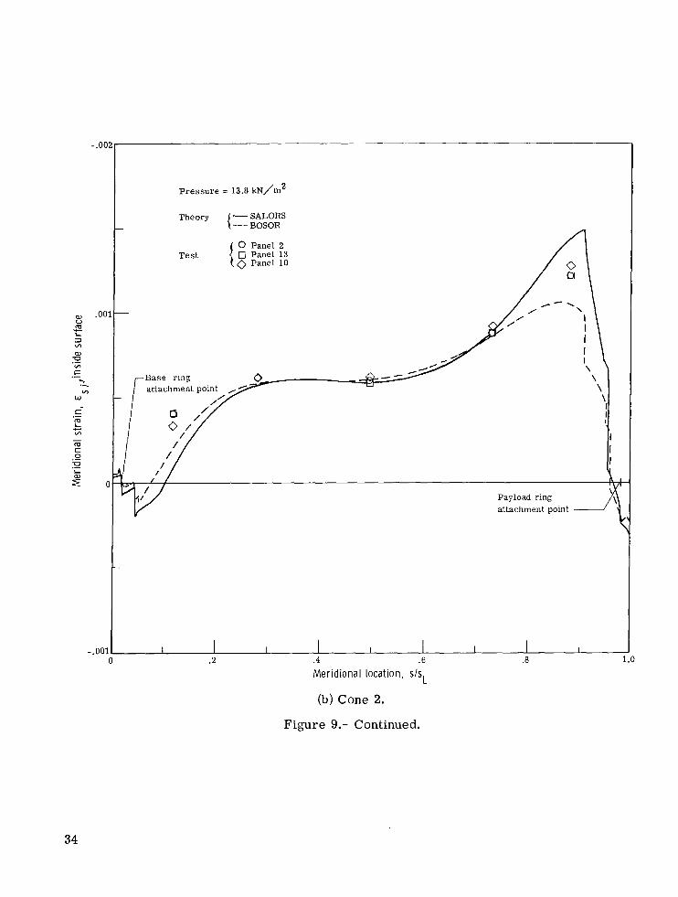
The prebuckling s t ra ins in the meridional direction along a meridional generator are shown in figures 8 and 9. generally good except near the inner edges where the maximum meridional bending moments occur.

The agreement between the programs and the tes t data is

The discontinuities in the theoretical curves predicted by BOSOR 2 are caused by using discontinuous wall construction near the ends and in the doubler region of the shell. In BOSOR 2, the doubler region was divided into equal segments, with each segment having a constant thickness obtained by averaging the thickness of adjacent segments. dix B.) However, in SALORS, the thickness was varied linearly ac ross the doubler region; hence, there are no jump discontinuities in the shell thickness and therefore no resulting jump discontinuities in the predicted s t ra in curves. The discontinuities at s sL = 0.01678 and 0.9832 in both curves are caused by the attachment of the base ring and payload ring, respectively.

(See appen-

1

The circumferential s t ra ins produced i n the base ring and payload ring at the prebuckling p res su re load of 13.8 kN/m2 (2.0 psi) for each cone are given in table 11. Strain gages A and B were attached to the rings along the s a m e meridional generator that was used in figures 6 to 9 for s t ra in data on the cone walls, each generator being 120° apart. The panel number and gage are noted on table II. The location of these panels with respect to each cone is given in appendix A.

7

Buckling Tes t s

The buckling character of all three cones was essentially the same with the development of a s ix full-wave buckle pattern (general instability) about the circumference of each cone. The buckling phenomenon was not catastrophic as the development of the buckles occurred smoothly and the shell remained intact. After each cone was buckled, the p re s su re loading was reduced to zero and each cone visually inspected on the outside. There appeared to be no damage to any of the cones from the buckling loading. Figures 10 and 11 show cones 2 and 3 at buckling. The depth of the buckles can be seen by the sepa- ration of the sandwich wall f rom the straight edges.

Tes t procedure for the buckling test called for all 12 panels of each cone to be instrumented with a sufficient number of s t ra in gages to determine wall bending and to anticipate the onset of buckling. These gages were placed back-to-back (outside and inside surface of sandwich walls) midway between panel s eams and at the meridional station in the vicinity of expected maximum deflection to measure circumferential s t ra ins . The s t ra ins in the panel exhibiting the most wall bending in each cone during the buckling tes ts are shown in figure 12.

The onset of buckling is defined in this report as that p re s su re at which there is s t ra in reversal (or m o r e exactly, a strain-rate reversal) in the circumferential s t ra ins in the buckling region. Sometimes the buckling load and collapse load (that is, that s ta te at which no additional load can be carried) of a s t ructure occur simultaneously o r so very close to each other that the collapse load, which is obviously easy to define, is assumed to be the same as the buckling load. An easily defined buckling load is not the case in the tests of the s t ructures of this report. None of the cones collapsed at buckling but continued to ca r ry additional load. Examination of figure 12 shows that at a certain p re s - s u r e for each cone, a p res su re plateau exists where a sizable change in s t ra in occurs with little increase in p re s su re . This p re s su re plateau is at the same p res su re level no matter what panel is examined around the cone and does not depend upon the relative magnitude of the wall bending between panels. These p re s su re levels for cones 1 , 2, and 3 a r e 41.7 kN/m2 (6.046 psi), 33.1 kN/m2 (4.800 psi), and 23.2 kN/m2 (3.371 psi), respectively. While the p re s su re plateau is easily identified from test results, a consistent s t ra in-reversal p r e s s u r e is difficult to determine. reversal p re s su re as determined from test pressure-s t ra in plots' was about 8.5 percent below the plateau value for each cone. The buckling p res su re was therefore assumed to be 8.5 percent below this plateau for each cone.

The average value of the s t ra in-

The buckling p r e s s u r e determined by this reduction procedure for cone 1 was 38.1 kN/m2 (5.53 psi), and the apparent buckling mode contained six circumferential waves. The horizontal o r radial displacement of the base ring at buckling was only a few thousandths of a centimeter inward; however, the vertical displacement was between

8

1.17 cm (0.46 in.) and 1.30 cm (0.51 in.) downward. was 30.3 kN/m2 (4.39 psi) with six circumferential waves and with a base-ring displacement of 1.12 cm (0.44 in.) to 1.17 cm (0.46 in.) downward and only a slight inward radial displacement. Cone 3 buckled at 21.2 kN/m2 (3.08 psi) and also had six circumferential waves with a base-ring displacement of 0.84 cm (0.33 in.) to 0.86 cm (0.34 in.) downward and again only slight inward displacement.

The buckling p res su re of cone 2

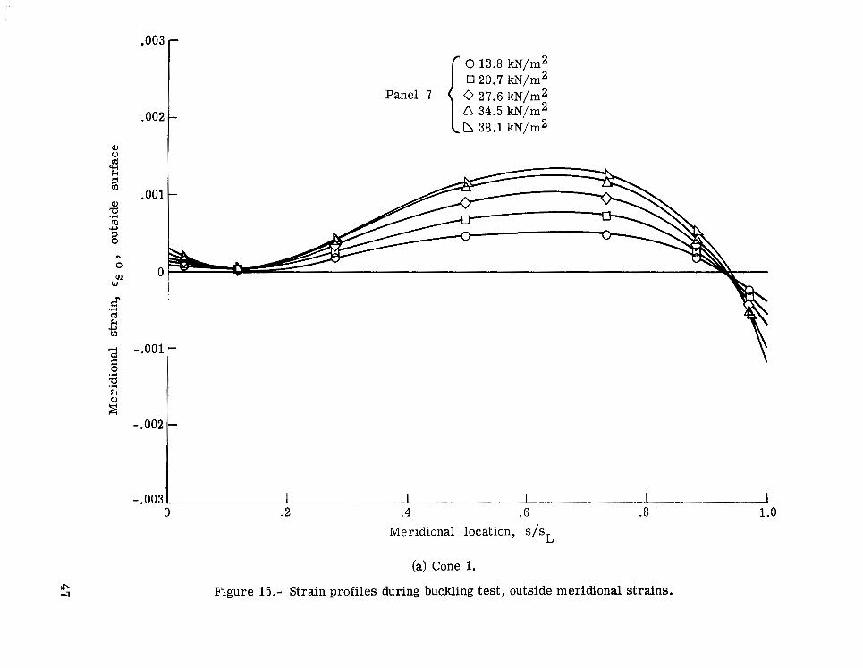
One panel on each cone was instrumented with a sufficient number of s t ra in gages to indicate the s t ra in profile at buckling. inside circumferential s t ra ins for the three cones and figures 15 and 16 present outside and inside meridional s t ra ins . Profiles are given for the buckling p res su re and also at several lower p re s su res for trend comparison. Test data are plotted a t discrete points as shown; however, a continuous curve was faired through these points to indicate the approximate s t ra in levels a t points where data were not taken.

Figures 13 and 14 present the outside and

Theoretical buckling predictions from BOSOR 2 and SALORS a r e given in table m along with tes t values. of six circumferential waves, although both buckling computer programs (BOSOR 2 and SALORS) predicted buckling modes of seven waves. may be responsible for the difference in the theoretically predicted mode and apparent tes t mode because of the closeness of the buckling p res su res €or the buckling modes of six and seven waves. into six circumferential waves; the node points of the waves were in close proximity to the seams joining adjacent panels.

All three cones buckled into an apparent general instability mode

Fabrication details of the tes t cones

(See appendix B.) Each cone was built f rom 12 panels and buckled

Theoretical buckling predictions for shells are usually higher than actual test resul ts . The BOSOR 2 analysis predicts a buckling p res su re that must be reduced by about 29 percent for cone 1 and by about 24 percent for cones 2 and 3. The SALORS anal- y s i s predicts a buckling p res su re that must be reduced by about 24, 20, and 19 percent for cones 1, 2, and 3, respectively. These reduction percentages a r e comparable to the 25-percent reduction recommended in reference 5 for this type of structure. are also comparable to the 20-percent reduction obtained from tests in reference 1.

These values

The tests also verified that the base rings were sufficiently stiff to prevent inexten- This problem had been studied ear l ier by Cohen. sional shell buckling. (See ref. 6.)

Postbuckling Tests

While the buckling of the three honeycomb cones was of a mild nature, the failure was of a violent, almost explosive nature. separate loading cycles; that is, after buckling, the cones were completely unloaded and then reloaded to failure. The pressure-s t ra in curves of figure 12 indicate the reaction

The buckling and failure tes ts consisted of two

9

II II I I" I 1111111111 II

of the selected panels on each cone to the two load cycles, buckling and failure. ling mode remained unchanged during the test from the initiation of s t ra in r eve r sa l until failure.

The buck-

Each cone maintained the ability to ca r ry additional p re s su re loading after buckling, as much as 48 percent more for cone 2 and as little as 18 percent more for cone 1, although both cones failed at approximately the s a m e p res su re . Cone 3 carr ied 30 percent more p re s su re after buckling. Figures 17 to 19 show photographs of the failed cones. All the cones were s t i l l able to withstand some load af te r failure with the exception of cone 2 which was ruptured a t failure.

CONCLUDING REMARKS

The test resul ts from an investigation to determine the buckling phenomenon and structural response caused by applied uniform external p re s su re on three honeycomb aluminum conical shells have been presented. These shells have dimensions applicable to space missions involving s t ructural decelerators o r aeroshells. Imperfection measurements were made on each cone and should be of benefit for further research into the effect of shell imperfections on the buckling of shells.

Tes t resu l t s were compared with two contemporary sophisticated shell-of- revolution analyses. The prebuckling s t ra ins agreed well with theory except in the region of the payload ring (small radius edge); there the test data generally fell between the two predicted s t ra in curves. All three cones buckled into a general instability mode with six circumferential waves.

Both analysis programs predicted a buckling mode of seven waves for each cone, compared with six circumferential waves in the tests; however, construction details of the cones may be responsible for this discrepancy. The BOSOR 2 analysis predicted a cr i t - ical buckling p res su re that should be reduced by about 30 percent for cone 1 (honeycomb walls with the thickest face sheets) and by about 25 percent for cones 2 and 3 for adequate agreement with tes ts . reduced by 25 percent for cone 1 and 20 percent for cones 2 and 3.

The SALORS analysis predicted cri t ical p re s su res that must be

The cones exhibited a substantial postbuckling strength carrying loads from 18 to 48 percent above the initial buckling loads; also there was no evidence of inextensional buckling at any load level.

Langley Research Center, National Aeronautics and Space Administration,

Hampton, Va., April 16, 1975.

10

APPENDIX A

SHELL SURFACE IMPERFECTION MEASUREMENTS

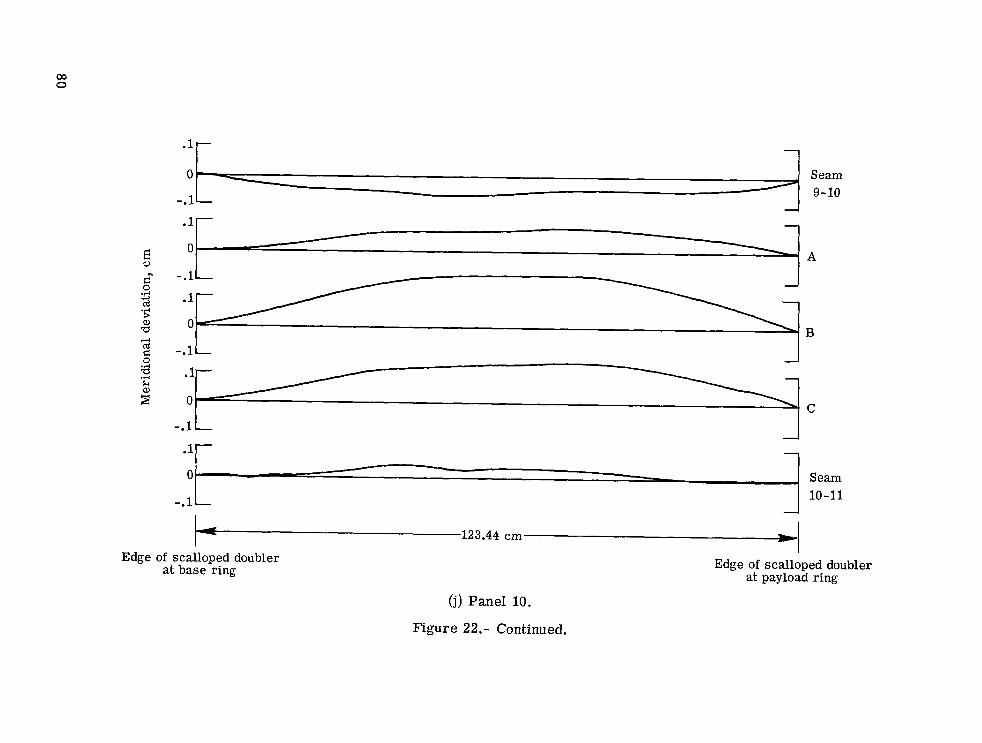
The conical shell surfaces of all three cones were measured extensively to determine the geometric imperfections present in an "as fabricated" and no-load condition. The distances from a straight meridian to the surface of the cones were established along meridional lines between the scalloped shell doublers located at each end of the cones. Measurements were taken at 7.5O intervals around the circumference in a counterclock- wise direction. Figure 20 shows locations on the panels where imperfection measurements were made and also shows meridional locations where s t ra in gages were installed for the prebuckling and buckling tests.

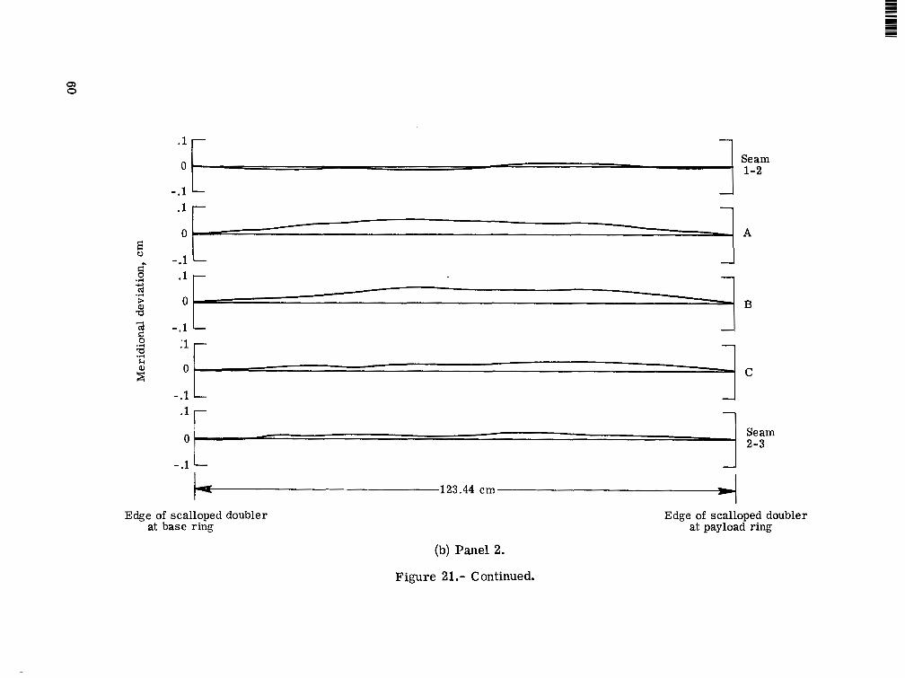
Figures 21, 22, and 23 present the imperfection measurements for each panel of the three cones. Each panel is numbered for reference in the text and figures.

Figure 24 shows the imperfection measurements around each cone circumference s = 75.18 cm (29.60 in.). a t the meridional station,

that was used in figure 12, the station of expected maximum deflection. each cone a r e bowed out between seams, with the seams being nearly on the nominal c i rc le of zero imperfections.

This is the same station location The panels on

11

APPENDIX B

PREBUCKLING AND BUCKLING ANALYSES FOR TEST CONES

Two computer programs, SALORS and BOSOR 2, were used to analyze the cones discussed in the text. A discussion and comparison of these programs are given in reference 7. Both systems employ finite-difference solution procedures; however, BOSOR 2 applies the difference approximations to the energy expression, whereas the SALORS program applies the difference approximations to the differential equations of equilibrium.

The theoretical predictions given in the text are based on the analytical models of the cones shown in figure 25. In the SALORS program a nonlinear analysis was used to compute the prebuckling s t ra in distributions, whereas a linear prebuckling s t r e s s state was used in the stability analysis. The SALORS nonlinear s t r e s s analysis option is unpub- lished, but the theory and u s e r ' s manual for the l inear s t r e s s analysis option is described in detail in reference 8. The external p re s su re loading was considered live (load remains normal to the deformed surface). The BOSOR 2 program is described in detail in reference 9. A nonlinear analysis was used to compute the prebuckling s t ra in distribution and also to compute the prebuckling s t r e s s state in the stability analysis. s u r e loading was not considered to be live.

External p r e s -

Numerical values used in the computations are given in tables I and IV. Table I contains the measured thicknesses obtained from many coupons cut f rom each cone. The adhesive was chemically dissolved and each coupon weighed. One layer of the uncured adhesive had a weight of 2.969 N/m2 (0.062 lbf/ft2) and a thickness of 0.030 cm (0.012 in.). The weight measurements showed that the average weight of one layer of the cured adhesive was about 2.825 N/m2 (0.059 lbf/ft2). To determine the actual thick- nes s of the adhesive in the tes t specimens, photomicrographs were taken of the sandwich wall c r o s s section for each cone. These a r e shown in figure 26. The bond thickness for each cone was approximately 0.025 cm (0.010 in.).

The mechanical properties used in the analysis are shown in table N. The in-plane stiffness for the wall of each cone was determined by tes t s on many compression coupons. The contribution of the co re and adhesive was considered to be the difference between the total stiffness of the coupon and that of the two face sheets. The adhesive was assumed to have an isotropic Young's modulus of 3.45 GN/m2 (0.5 X 106 psi) and a Poisson's ra t io of 0.35. (See ref. 10.) The nonwoven synthetic fabric adhesive car r ie r , upon inspection, was considered ineffective in carrying load. Because of its small extensional stiffness, the honeycomb core was a l so considered to be isotropic with the same Poisson's ra t io as that of the adhesive.

12

APPENDIX B - Concluded

Figure 27 is a plot of the buckling p res su re as a function of buckling mode number as computed by BOSOR 2 for its analytical model. The closeness in the buckling p res su res for the buckling modes of 6 and 7 was apparent, thus lending credibility to the assumption that the construction details of the tes t cones may have affected the buckling modes.

Stiffness measurements of the compression coupons also indicated that there was no discernible difference between the coupons cut from the failed cones and the coupons from the unloaded extra panel.

13

REFERENCES

1. Anderson, J a m e s Kent; and Davis, Randall C.: Buckling Tests of Two 4.6-Meter- Diameter, Magnesium Ring-Stiffened Conical Shells Loaded Under External Pres- sure. NASA TN D-7303, 1973.

2. Heard, Walter L., Jr.; Anderson, Melvin S.; Anderson, J a m e s Kent; and Card, Michael F.: Design, Analysis, and Tests of a Structural Prototype Viking Aero- shell. J. Spacecraft & Rockets, vol. 10, no. 1, Jan. 1973, pp. 56-65.

3. Williams, J e r r y G.; and Davis, Randall C.: Experiments on Stiffened Conical Shell Paper No. 2268A, SOC. Exptl. S t ress Analy- Structures Using Cas t Epoxy Models.

sis, Oct. 1973.

4. Metric Practice Guide.

5. Buckling of Thin-Walled Truncated Cones. NASA SP-8019, 1968.

6. Cohen, Gerald A.:

E 380-72, Amer. SOC. Testing & Mater., June 1972.

The Effect of Edge Constraint on the Buckling of Sandwich and Ring-Stiffened 120 Degree Conical Shells Subjected to External Pressure . NASA CR-795, 1967.

7. Anderson, M. S.; Fulton, R. E.; Heard, W. L., Jr.; and Walz, J. E.: S t ress , Buckling, and Vibration Analysis of Shells of Revolution. Computers & Structures, vol. 1, nos. 1/2, Aug. 1971, pp. 157-192.

8. Heard, Walter L., Jr.; Anderson, Melvin S.; and Chen, Ming M.: Computer Program for Structural Analysis of Layered Orthotropic Ring-Stiffened Shells of Revolution (SALORS) - Linear S t ress Analysis Option. NASA TN D-7179, 1973.

9. Bushnell, David: Buckling and Vibration of Segmented, Ring-Stiffened Shells of

(Available Revolution - User 's Manual for BOSOR 2. N00014-67-C-0256), Lockheed Missiles & Space Co., Sept. 1968. from DDC as AD 863 453.)

LMSC 6-78-68-40 (Contract

10. Ashton, J. E.; Halpin, J. C.; and Peti t , P. H.: P r i m e r on Composite Materials: Analysis. Technomic Pub. Co., Inc., c.1969.

14

TABLE 1.- MEASURED STRUCTURAL DIMENSIONS

- __ Stiffening rings Honeycomb wall

Base ring wal l thickness

Face sheets average thickness

Honeycomb co re height Payload ring

all thickness loneycomb wall, total thickness Cone

1

2

3

in.

0.500

0.500

0.500

in.

0.127

0.127

0.127

’ in.

0.157

0.157

0.157

in.

0.0196

0.0143

0.0096

em

0.323

0.323

0.323

_ - cm

0.399

0.399

0.399

cm

0.0498

0.0363

0.0244

cm

1.270

1.270

1.270

TABLE II.- CIRCUMFERENTIAL STRAINS IN THE END RINGS

AT 13.8 kN/m2 (2.00 psi)

Base ring Payload ring Cone

1

2

3

or E Panel

7

11

3

2

13

10

2

6

10

G a g e

A B A B A B

A B A B A B

A B A B A B

Gage Panel

7

11

3

2

13

10

2

6

10

A

////////// A B A B A B

A B A B A B

- 0.000004 .000083

- .000006 .000071 .000005 .000073

0.000013 .000086 .000003 .000089 .000010 .000084

0.0000 19 .000128 .000023 .000123 .oooo 11 .OOO 113

-0.00049 1 .000789

-.000162 .000787

- .ooo 190 .000832

. Payload _- ring

-0.000221 ,000821

-.000106 .000695

-.000055 ,000829

-0.000 100 .000675

-.000317 .000870

- .000122 .0008 14

A B A B A B

B Base ring

15

I

I l11111111111111~11111l111111 I

n . W / m 2

n

7 50.06 7 53.78

7 37.99 7 39.85 . . .

TABLE m.- BUCKLING RESULTS FROM TESTS AND THEORY

psi

7.80

5.78

Tes t s

30.27

21.24 _- -

_ _ - . ".

. .

psi

5.53

4.39

3.08 -

TABLE 1V.- MECHANICAL PROPERTIES USED IN THE CONE ANALYSIS

[Young's modulus for the magnesium rings was taken to be 44.8 GN/m2 (6.5 X l o6 psi)]

Face sheets Property

a Reference 10.

Material

Adhesive a

3.45 (0.50 x 106) 1.28 (0.185 X 106)

.35

Honeycomb c o r e b I 0.262 (0.038 x 106)

.097 ( .014 x 106)

.35

-

b The experimentally determined total stiffness of the core (adhesive and honeycomb core) was the same for each cone, that is, 4.90 MN/m (28 x lo3 lb/in.).

16

I

449.58 cm (177.00 in)

4 - Figure 1.- Cross section of test cones showing shape and design test loading.

4

,

*.I . "

L-69-5235 (a) Outside view of cone 2.

Figure 2.- Overall view of test cone.

L- 69- 5234 (b) Inside view of cone 2.

Figure 2.- Concluded.

19

N 0

3

1.251 l r i ternal wrenching ews 1.91 (.751 apart

,953 (.375)

Payload r i n g wi th 6.35 12.50) 0. 0. and wall th ickness of .318 (.1251

100.33 139.501 R+--

Section A-A

.025(.010)

wi th 15.24 16.00) wall th ickness of

Section B-B

m\ ,038 1.015)

Top View

Honeycomb sandwich cone

Figure 3.- Construction details of test cones. Dimensions given in cm (in.).

-30.48 112.00-

k-15.24 (6.001-

w Detail A

d d 7 - n 6.35 12.501 -7

-----

.79 1.31) Detail B

3.81 (1.50)

1.27 1.50)

r ivets Jo in t between adjacent panels t

doubler

Section C-C View D-D


t

,-- Payload ring j Flat machined surface of steel conical test fixture Flat machined surface of steel conical test fixture

Vacuum

-Support legs - ring

I /

# Vacuum I I1

chamber 7 Test--\ cone

Figure 4.- Cross-section schematic view of test setup.

L- 69-8555.1 Figure 5.- Test setup components excluding test cones.

N w

2 Pressure = 13.8 kN /in

- SALORS BOSOR 2

0 Panel 7

9 Panel 3 T e s t I 0 Panel 11

I I I - 1 .4 .2 -.001

0 I

Test ' Cone

Q

1 Meridional location, s/sL

(a) Cone 1.

Figure 6.- Comparison of tes t and theoretical circumferential s t ra ins on outside surface. (See fig. 20 for panel numbering system.)

24

.oo

.oo

.oo

P r e s s u r e = 13.5 kN/m2

SALORS Theory { -- BOSOR 2

0 Panel 2 Test 1 0 Panel 13

0 Panel 10 <-$e, T e s t I Cone

Q

I 0

Meridional location, s l s ,

(b) Cone 2.

Figure 6.- Continued.

25

.oo:

.oo

-.oo

-.oc I

.

I

Pressu re = 13.8 kN/M"

SALORS Theory (T- BOSOR 2

O Panel 2 Test I 0 Panel 6

0 Panel 10

0

(c) Cone 3.


26

.oo

. O(

- .Ol

P r e s s u r e = 13.8 k N / m 2

SALORS Theory { :_ BOSOR 2

0 Panel 7 0 Panel 11

anel 3

I I .2

1 I ~I I I .E .4 . t i

Meridional location, s/sL

(a) Cone 1.

0

Figure 7.- Comparison of tes t and theoretical circumferential s t ra ins on inside surface.

27

I I I

2 Pressu re = 13.8 kN ni

SALORS BOSOR 2 Theory { -__

0 Panel 2 Test I 0 Panel 13

panel 10

Meridional location, s/sl

(b) Cone 2.


28

.oo:

.oo

' I

- ,001

- . 00:

P r e s s u r e = 13.8 kN /m2

SALORS BOSOR 2

0 P a n e l 2 Test I 8 Panel 6

- Theory { _ _ -

Panel 10

0

I 1 1 1 I I I I I .E .6 .4

Meridional location, s/sL .2 3

(c) Cone 3.


29

.002

,001

P r e s s u r e = 13.5 kN / m 2

SALORS BOSOR 2

Payload ring attachment point

I - - .J- - - 1 . - I I -.001 , 0 . 2 .4 Merid ional location, s/sl .6

(a) Cone 1.

Figure 8.- Comparison of tes t and theoretical meridional s t ra ins on outside surface.

30

Q) u m

L

3 VI

Q) U VI

2

c

.- c

9 0 VI

W

.- m L c VI

m t 0

-

.- E I

2

.01

.o

-.oc

2 P r e s s u r e = 13.8 kN/ m

SALORS Theory { BOSOR 2

0 Panel 2 Tes t 1 g Panel 13

Panel 10

Payload ring attachment- point

\-Base ring attachment point

I 1 I .2

I I I 1 1 I 1 I I

.4 .6 .8 I Merid ional location, s l s

(b) Cone 2.

L

0


31

a, u m - I

3 VI

al

VI

3 0

E c

0 VI w

S-

m, .- c VI

m c 0

- .- E I

f

I

.Ol

I I I I

.O(

-.O(

-.oo

2 P r e s s u r e = 13.8 kN/m

Theory - SALORS I---BOSOR 2

0 Panel 2 Payload ring

0 Panel 10 attachment T e s t I 0 Panel 6

' -1 attachment point

32

Pressure-= 13.8 kN/m2 SALORS

Theorv {--- BOSOR 2

- -

T e s t

:i, \

LBBase ring attachment point Payload ring attachment point---/ ’(

0

Figure 9.- Comparison of test and theoretical meridional s t ra ins on the inside surface.

I.1- ~. . I 1 1 I I 1

I .E

1. .6 .2 .4

L Mer id iona l location, s l s

(a) Cone 1.

33

- . 00:

I I

Q) .001 V m -

I I I

L

3 VI

a, -a VI c .- .-

4 .- v)

W

c m I c VI

m c 0

.-

-

.- E I

9 0

-.001 (

P r e s s u r e = 13.8 kN/m2

Theory SALORS

0 Panel 2 0 Panel 13 0 Panel 10

T e s t {

-

Base ring

Payload ring attachment point

34

00

OC

a, V m L 3 m

a , +

m

c

E c .- . .-

v) W

c .- =I c m

m c 0

- .- E L

9

-.O(

-.O(

SALORS BOSOR 2

. Base ring attachment point

0 Panel 2 Test I 0 Panel 6

0 Panel 10

.2 .4 .6

Meridional location, s l s L

( c ) Cone 3.


.8 1.0

35

w Q,

L- 69- 60% Figure 10.- Buckled cone 2. (Pressure maintained to hold buckle pattern.)

Figure 11.- Buckled cone 3. (Pressure maintained to hold buckle pattern.)

w 4

Pressure, m / m 2 (psi)

50.00 (7.25)

40.00 '(5.80)

30.00 - (4.35)

- 20.00 (2.90)

- 10.00 (1.45)

2 Ultimate pressure 45.51 kN/m (6.60 psi) -- 2

-- -I- Assumed experimental buckling pressure 38.13 kN/m (5.53 psi) 2

pailu r e test

.003 .002 .001 0 - . O O 1 -.002 -.003 -.004 -.005 -.006 -.007 -.008

Circumferential strain

(a) Cone 1.

Figure 12.- Pressure-strain relationship at center of panel exhibiting the most wall bending.

Pressure kN/m2 (psi)

- 50.00 (7.25)

30.00 (4.35)

20:oo (2.90)

.10.00 (1.45)

.003 .002 .001

2 Ultimate pressure 44.40 kN/m (6.44 psi)

---- Assumed experimental buckling pressure 30.27 kN/m (4.39 psi) 2

Panel 8

1 1 1 1 1 1 1 1 -.001 -.002 -.003 -.004 -.005 -.006 -.007 -.008


(b) Cone 2.


50.00 (7.25)

- 30.00 (4.35)

- 20.00 (2.90)

10.00 - (1.45)

2 Ultimate pressure 27.30 kN/m (3.96 psi) -- 7 --------

essure plateau 23.24 kN/m 2 (3.37 psi)

d experimental buckling 2

------

pressure 21.24 kN/m (3.08 psi)

Panel 4

I I J I I I I I I I .003 .002 .001 0 -.001 -. 002 -.003 -.004 -.005 -.006 -.007 -.008


(c) Cone 3.


I

.003 -

.002 -

.001

0

- .001

- .002

2 0 13.8 kN/m2 0 20.7 kN/m2 0 27.6 kN/m2 A 34.5 W/m2 b 38.1 kN/m

1.0

a, 0 cd k w

2 2 a,

m 3 0

U

L

0 ca

w

c cd k m

cd

c a k a,

s 0 k

u

- .rl

U

4

.rl U

3 .rl

.003

.002

.001

0

-.001

- ,002

-.003

0 13.8 kN/m 2

A 30.3 kN/m 2

0 20.7 kN/m2 0 27.6 kN/m2

Panel 2

I I I I .2 .4 .6 .8 1.0

I Meridional location, s/sL

(b) Cone 2.


,003

.002

.001

0

. - 001

-. 002

21.2 kN/m 1 O 13.8

I I I I I 0 .2 .4 .6 .8 1.0 -.003


(c) Cone 3.


I I I I I 0 .2 .4 .6 .8 1.0 -.003


(c) Cone 3.


W

+I k 5 m a,

m E:

2

2 .r(

w.

.d

m W

.Er cd k m U

.002

. O O l

0

I 4

.r( cd

2 - . O O l L

E ~ a ;

W k W I w

k .4

0 13.8 kN/m 2

0 2 7 . 6 kN/m2 0 20.7 kN/m2

A 34.5 kN/m2 b 38.1 kN/m2

- .003 I I I I I I .2 .4 .6 .a 1.0 0


(a) Cone 1.

Figure 14.- Strain profiles during buckling test, inside circumferential strains.

.003

.002 a, 0

3 3 m a,

m E: 2 .001 .rl

r.

.rl

m W

0 .g cd k m

cd

u

4

.rl Y

E: -.001 a, k a,

3 0 k

2 .d

v -.002

0 13.8 kN/m2 0 20.7 kN/m2 0 27.6 kN/m2 A 30.3 kN/m2

Panel 2

I I I I I .2 .4 .6 .8 1.0 -.003

0 Meridional location, s/sL

(b) Cone 2.


a, 0 cd

Y-( k 9 m a,

m d 2 .3

n .r(

m w

.$ nl k m

cd

U

H

.-I

,003

.002

.003

(

3 0 k .d

u - .002

-.003

,/ 013 .8 kN/mi 021.2 kN/m

I I I I I 0 .2 .4 .6 .8 1.0


(c) Cone 3.


0, 0 rd +I k 5 v1

al

v1

5 0

2 U

A

0 m

W

d .r(

cd k v)

cd

U

I 4

.r(

2 k

i

,003

.002

.001

0

-.001-

I1 I

0 13.8 kN/m2 0 20.7 kN/m2 0 27.6 kN/m2 A 34.5 m / m 2 b 38.1 kN/m2

(a) Cone 1.

Figure 15.- Strain profiles during buckling test, outside meridional strains.

.003

.002

.001

0

-.001

- .002

0 13.8 kN/mi

0 0 27.6 20.7 kN/m kN/mi A 30.3 kN/m

.003

.002

aJ 0 cd w k 5

Q)

m s 0

.001 3 U

n

0

W “ 0 n

9 k m

cd

42

I+

g -.001 5 3 k

- .002

-.003

O 21.2 13.8 m/m2

I I I I 1


(c) Cone 3.


" W n

3 k m -c,

L 1

-.001 0

k 5 s

-. 002

- .003 I I I I I I 0 .2 .4 .6 .8 1.0

Meridional location, s/s

(a) Cone 1.

Figure 16.- Strain profiles during buckling test , inside meridional strains.

.003

.002

cu

+I s g .001

2 : W " 0

k

cu

.PI

n

.rl

I=" .PI cd k [D U

,+ : -.001 0

k

.rl

2 i

-.002

- .003 I I I I 1 0 .2 .4 .6 .8 1 .o


(b) Cone 2


.003

- .003

.002

I I I I J

a, u cd +I k s II) .001

m W 0

4 cd c 0

k

- .001 .A

2 i

- .002

L-69-6096.1 (a) Overall view.

Figure 18.- Failure of cone 2. pult = 44.40 kN/m2 (6.44 psi).

*" i .

L-69-6089 (b) Close-up view of ruptured area.

Figure 18. - Concluded.

55

- - (a) Outside overall view.

Figure 19.- Failure of cone 3. pult = 27.30 IrN/m2 (3.96 psi).

c

< P

L-75-150 (b) Inside close-up view.


rMeridian for prebuckling and buckling strains Meridian for prebuckling strains 7

'Mer id ional I i nes

CONE 1 CONE 2

Meridian for prebuckling strains

*Strain gages are located along t he B meridian.

Meridian for prebuckling strai

13.97 cm (5.50 in.)

Meridian for prebuckling and buckling Base strains ring

CONE 3

Figure 20.- Panel orientation and imperfection measuring details for cones 1, 2, and 3.

1

-.l .1

2

-.l

0

- - - -

0 -

Inward deviation - -

-.l L Outward deviation J /-- -

Edge of scalloped doubler at base ring

Seam 13-1

A

B

C

Seam 1-2

Edge of scalloped doubler at payload ring

(a) Panel 1.

Figure 21.- Imperfection measurements of cone 1.

Q, 0

.1

-.l .1

- - O--

- -

- - 0 - - I

-.l I

0 -

-1

1

.'l

-.l .1

0

-.l

- - 0- I

- -

- -

r r -

-


Seam 1-2

A

B

C

Seam 2-3

Edge of scalloped doubler a t payload ring

(b) Panel 2.


.1 - 0- I

-

- .1

0

-

- .1 - 0 - -

A

-.l L J

-.l L J


Seam 2-3

A

B

Seam ' 3-4


( c ) Panel 3.


.1

0

-.l .1

E o 0

g -.l .r( 4 2

.d cd -1

2 0

0 -.l 2 .1

>

+ cd E: .r(

k

2 0

-.l .1

0 - Seam - 4-5

I 1



(d) Panel 4.


r 0- L

7

0 -

k P

c 0

-.l .1

2 - - - -

k

-.l - .1 -

5 - -


Seam 4- 5

A

B

C

Seam 5- 6


(e) Panel 5.


Q, w

.1 - 0 -

-.l - .1 - 0-

-

- - -

II

E v -.l L

Seam 5-6

- A

- 0

4--

.d c)

.rl cd k. 0 - -B

g .1 z .d

k

-.l .1

0

-.l

5

123.44 cm _I

- - 0- - c - - - -

Seam - - 6-7

- -



(f) Panel 6.


-.l .1

0 E u

-.l .1

0

-.l

r 1

L

r _1

1


Seam 6-7

A

B

C

Seam 7 -8


(g) Panel 7.


0 1 Seam 7-8

- -

0

- -

-.l L _I

A

-.l - - .1 - -

0 -


C


0 -=- -

(h) Panel 8.


Seam 8-9

-.l -

< 123.44 cm _j

.1

0

-.l .1

0

E -.l 0

C 0

cd

a,

h .1

0 .d U

.c= = -.l

.1 ;;I C 0 .d

3 k 0

; -.l .1

0

-.l

r 1

L

L

r J

1

1_ 123.44 cm


Seam 8-9

A

B

C

Seam 9-10


(i) Panel 9.


.1 - -

/ 0- - / - =

-.l - .1 - 0-

- -

E -.1- 4


Seam 9-10

A


7 .I .I -

e 0 .rl

U cd 0- ‘5 W ‘CI 4

(j) Panel 10.


B

-.l .1 74

2 0

e 0

k

.,-I

s

- - - - - C

i

- 0-

-

Seam 10-11

.1

-

r 1 0

-.l .1

E 0 0 n

0 d -.l

*$

.A U .1

0

cd

a m -2 0 -. 1 2 .1

d .A

k s 0

-.l .1

0

-.l

L

L -J

r -1

Edge of scalloped doubler a t base ring

Seam 10-11

A

B

C

Seam 11-13


(k) Panel 11.


4 0

- Seam - 11-13 0-

9 - 0-=------ A

-.l - I

-- Seam 0-- 13- 1

123.44 cm -

-.l 1

-.l L r

J 1



(1) Panel 13.

Figure 2 1. - Concluded.

.l- - 0-

1 -

-.l _I

-.l L r

_I 1

Seam 12-1

A

B

C

Seam 1-2 0-

Inward deviation 1 -.1- -

123.44 cm



(a) Panel 1.


E 0

c 0

cd

a, a

c 0

I

.rl U

.Fl

2

3 3

-

0 1 - Seam 1-2

-.l L

0

J

A

- 0 - B

-.l L

-.1-

-.1-

.l- CI

Seam 0- 2-3

- 4 123.44 cm



(b) Panel 2.


-1 r 1

Seam 2-3 0;-

E u c 0

n

.d U s al P

cd c 0

k

4

.r(

2 2

0 Seam - 3-4

-.l -I

-.l _J -

B

-.l L

-.l L J . 123.44 cm


( c ) Panel 3.



4

Seam

-.l L A

3-4

-.I -!

0 -

1

- 5 A

-.1- -

123.44 cm . .


Seam 4-5


(d) Panel 4.


.l-

0 . - -.1- .l-

-

- -

0~

-.1L

Seam 4-5

A

-.l L

~ 0

J 1

Seam 5-13

-.l L 123.44 cm



(e) Panel 5.


r

0 - 1

1

-.l

E 0

c 0

cd

a -a

n

.rl 0

'5

;;1 !?I

2 .rl

k s -

Seam 0- 13-14 - -

0

-.l .1

0

-.l .1

0

-.l .1

L r

J 1

r 1

Seam 5- 13

A

B

C



(f) Panel 13.


E u C 0

cd

a m cd C 0

n

.d 0

'5 d

5 2 k

-

0-

-.1- - Seam 13-14

0

-.l _1

0

-.1-

-.l J

Seam 14-8 0-

-

1 0

-.l .11-

_1

1 . 123.44 cm



(g) Panel 14.


-J W

0- 1

.1

0

1

E 0 A

Seam 14-8

.l- - 5

0- ~C

n L d 0 .r( -.l i

L d 0

-.l .+ 2 J

Seam 8-9

-.1L _I

L 123.44 cm _I Edge of scalloped doubler

a t base ring Edge of scalloped doubler

at payload ring

(h) Panel 8.


-.1-

0

-.1-

k k 1 2 3 . 4 4 cm -I

.l- - 0 - Seam

8-9 -

.l- - - - = = A

.l- - -


0

- .1-

-.1-

0


B

- .l- -

- c 0-

.l- - -

Seam

(i) Panel 9.


-.l- 2

9-10

CQ 0

r 1

0 -

-.1-

- . l I 0

-.l L .ll-

0

-.1L

123.44 cm


Seam 9-10

A

B

C

Seam 10-11

I


(j) Panel 10.


1 7 1

0- Seam 10-11

.I 1- 1

1 Seam 11-12 0-

-.l L J 123.44 cm t



(k) Panel 11.


0- - Seam

-.l L

E

_I 11-12 -

0 - = \ - A

Y cd

a, .m '5

tj I l

- 0- B

n -.1L

2 s k

-.1-

-.1-

.l-

0- C

-

- .l- -

/

0-

-

;;i B -.1L J


Seam 12-1


(1) Panel 12.


Seam

-.l L

*l I_

c

L-Inward deviation -.1-

.l-

0--

- -

,-Outward deviation

12-1

A

_1

1 / 0- - -B

-.1-

.11- 1

.l-

0-

-

F -

0 C

Seam 1-2

-.l L J

-.1-

4 123.44 cm



(a) Panel 1.


03 w

-.1-

E n -.1-

0

F: 0

cd

a, -a

.rl U

0 ??-

3 -.1-

s E! .rl k

-.1-

1

.l- - O w - - . l -

0-

- -

4

.l- 1

.l-

0-

- -

-

08


-

Seam 1-2

A

B

C

Seam 2-3


(b) Panel 2.


.11- 1

.1- -

0- - A E u

Seam 0 2-3

L4

J

-.1L 1

0- C

.a -.1L c 0

.l- .r( 4 4

d ' S m 0

3 d -.l L 0 z! .11- 1

-.1L J .1 -

Seam -.l O[\ - 3-4

k k 1 2 3 . 4 4 cm - - Edge of scalloped doubler

a t base ring Edge of scalloped doubler

at payload ring

(c) Panel 3.


m Q,

1

r 1

cd -.l I-

k a, "r

J 1

-

k k 1 2 3 . 4 4 cm m


Seam 3-4

A

B

C

Seam 4-5


(d) Panel 4.


-.l .1

u E O ; -.l s .1 '5 g o 1 8 -.l 2 .1

i o

0

cd

.A

k

-.l .1

0

-.l

0

-

r 1

r- 1

-1

1

L

I-

1

1


Seam 4-5

A

B

C

Seam 5-6


(e) Panel 5.


E 0

-.1-

-.1- .1

-.l

-.1-

d

'S

0

cd

0) a

.r( Y

. 1 7 -

o--- -~

4

.l- - 0-

- - -

0- -

- - .l- -.

0- 4

2

3

-.1-

0-

123.44 cm L,

-


Seam 5-6

A

B

C

Seam 6-7


(f) Panel 6.


-.1-

0 E .-, -.1- E

0


Seam 6-7 0-

.l-

0- A

- -

-


.l- -

.d U

.l- -2

2 .l- :

- a,

cd E

-0 0-

0 -.1,

l-4

.r( - k -

0-

-.1-

.l-

0;-

- -

-.1- -

T 123.44 cm - (g) Panel 7.


B

C

Seam 7-8

CD 0

k

5

4- 1

-

0- C

Seam 7-8 0

-.1L -I .l-

E A 0 n s -.1L i

-.1L .lr

J 7



(h) Panel 8.


T

E

E n

0

-I

0-

.l- e, P

c 0 ;;i 0

2 -.1-

3

- - - k

.l-

.o ~

-.lL .;i cd U

-.l L J

-.1- . 123.44 cm


Seam 8-9

A

B

C

Seam 9- 10


(i) Panel 9.


-.1-

E

C -.1-

'$

74

0 L

0

cd

W

.H 4 2

.I- - 0-) Seam

9-10 -

.l- -

0 - A

- .l- I

0- B

-.lL _1

.?-I k

f

Seam 10-11'

0

-

- c 0-

-.1L



(j) Panel 10.

Figure 23. - Continued.

-l r

u L

0 c -.1- .+ U

1

-

4 cd c 0 -.1-

.l- 2 -

k -

-.l L a i r

0.

1

- 0-


Seam 10-11

A

B

C

Seam 11-12

doubler Edge of scalloped . at payload ring

(k) Panel 11.


CD w

E 0

- Seam - 11-12 0-

.. c 0

cd

Q, Ti

.* U

'5

-.I- -

- - B O b

0- C

Seam 12- 1

- I 123.44 cm



(1) Panel 12.


(a) Cone 1.

Figure 24.- Imperfection measurements at the meridional station. s = 75.18 cm (29.60 in.).

95

I --

(b) Cone 2.


96

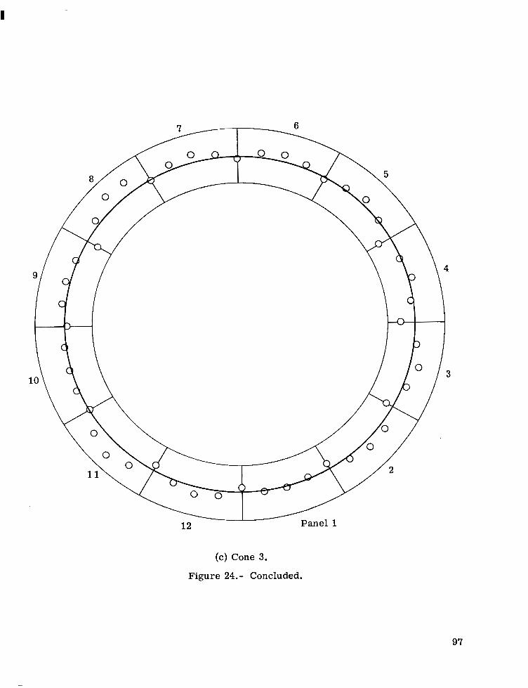
( e ) Cone 3.


97

4 Cone

reaction force I

k- 231.14 191.00) -uA-t

+ x Axial

t

OveraI I dimensions and loading of analytical model

Payload end sections as used in the programs SALORS and BOSOR 2 are shown at right. Base ring end is identical to payload end except for radius

Figure 25.- Analytical models

* h includes thickness of adhesive

for program analyses. Dimensions given in cm (in.).

. .

(a) Cone 1, panel 3. (b) Cone 2, panel 13.

(c) Cone 3, panel 10.

Figure 26.- Photomicrographs of honeycomb sandwich walls. Magnification X 63.

L-75-151

99

I -

L W

yl

0 I 1 I 1 I I I 2 3 4 5 6 7 8 9

Circumferential buckling wave number, n

Figure 27.- Buckling pressure as a function of buckling mode, as computed by BOSOR 2.

NATIONAL AERONAUTICS AND SPACE ADMINISTRATION WASHINGTON. D.C. 20546

P O S T A G E A N D FEES P A I D N A T I O N A L A E R O N A U T I C S A N D

SPACE A D M I N I S T R A T I O N OFF1 C I AL BUS I N ESS PENALTY FOR PRIVATE USE w o o SPECIAL FOURTH-CLASS RATE 451

BOOK

730 001 Ci Ij OEPT OF THE A I R FORCE

,- A F WEAPONS LABORATORY ATTN: TECHNICAL L I B R A R Y KIRTLAND A f f 3 NH 87117

D 750?111 S O 0 9 0395

[SUL)

P O S T ~ A S T ~ R : If Undeliverable (Section 158 Postal Manual) Do Not Return

______ -- - ~-

“The aeronautical and space activities of the United States shall be conducted so as to contribate . . . t o the expansion of human knowledge of phenomena in the atmosphere and space. T h e Administration shall provide for the widest practicable and appropriate disseminution of information concerning its activities and the results thereof.”

-NATIONAL AERONAUTICS AND SPACE ACT OF 1958

NASA SCIENTIFIC AND TECHNICAL PUBLICATIONS TECHNICAL REPORTS: Scientific and technical information considered important, complete, and a lasting contribution to existing knowledge.

TECHNICAL TRANSLATIONS: Information published in a foreign Janguage considered to merit NASA distribution in English.

- TECHNICAL NOTES: Information less broad in scope but nevertheless of importance as a contribution to existing knowledge.

TECHNICAL MEMORANDUMS: Information receiving limited distribution because of preliminary data, security classifica-

PUBLICAT1oNS: Information derived from or of value ro NASA activities. Publications include final reports of major projects, monographs, data compilations, handbooks, sourcebooks, and special bibliographies.

TECHNOLOGY UTILIZATION PUBLICATIONS: Information on technology

interest in commercial and other- non-aerospace applications. Publications include Tech Briefs, Technology Utilization Reports and Technology Surveys.

tion, or other reasons. Also includes conference proceedings with either limited or unlimited distribution.

CONTRACTOR REPORTS : Scientific and technical information generated under a NASA contract or grant and considered an important contribution to existing knowledge.

- used by NASA that may be of particular

Details on the availability of these publications may be obtained from:

SCIENTIFIC AND TECHNICAL [NFORMATION OFFICE

N A T I O N A L A E R O N A U T I C S A N D S P A C E A D M I N I S T R A T I O N Washington, D.C. 20546

Buckling tests of three 4.6 meter diameter alluminum honeycomb ...

Documents

Transcript of Buckling tests of three 4.6 meter diameter alluminum honeycomb ...