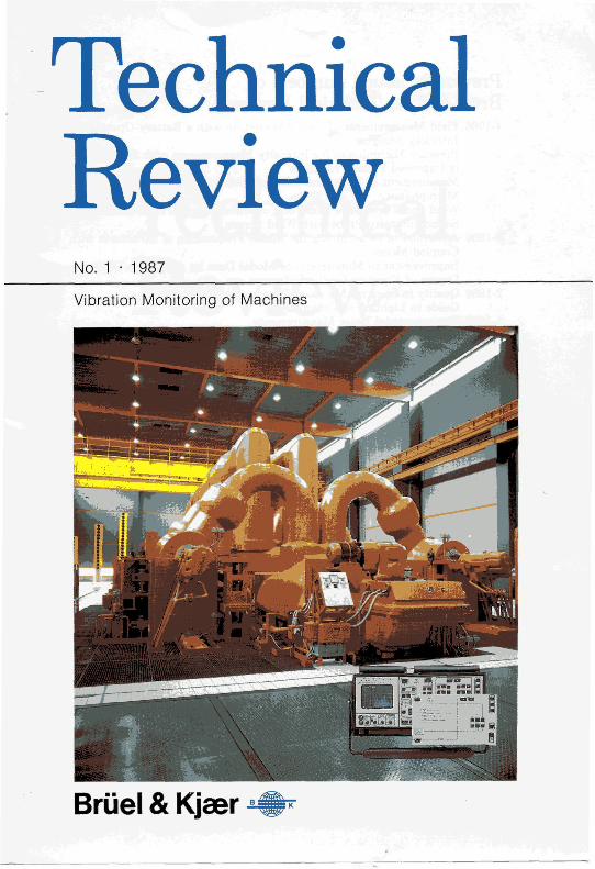
No. 1 -1987

Vibration Monitoring of Machines

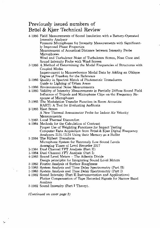
Previously issued numbers of Briiel & Kjser Technical Review 4-1986 Field Measurements of Sound Insulation with a Battery-Operated

Intensity Analyzer Pressure Microphones for Intensity Measurements with Significant­ly Improved Phase Properties Measurement of Acoustical Distance between Intensity Probe Microphones Wind and Turbulence Noise of Turbulence Screen, Nose Cone and Sound Intensity Probe with Wind Screen

3-1986 A Method of Determining the Modal Frequencies of Structures with Coupled Modes Improvement to Monoreference Modal Data by Adding an Oblique Degree of Freedom for the Reference

2-1986 Quality in Spectral Match of Photometric Transducers Guide to Lighting of Urban Areas

1-1986 Environmental Noise Measurements 4-1985 Validity of Intensity Measurements in Partially Diffuse Sound Field

Influence of Tripods and Microphone Clips on the Frequency Re­sponse of Microphones

3-1985 The Modulation Transfer Function in Room Acoustics RASTI: A Tool for Evaluating Auditoria

2-1985 Heat Stress A New Thermal Anemometer Probe for Indoor Air Velocity Measurements

1-1985 Local Thermal Discomfort 4-1984 Methods for the Calculation of Contrast

Proper Use of Weighting Functions for Impact Testing Computer Data Acquisition from Briiel & Kjser Digital Frequency Analyzers 2131/2134 Using their Memory as a Buffer

3-1984 The Hilbert Transform Microphone System for Extremely Low Sound Levels Averaging Times of Level Recorder 2317

2-1984 Dual Channel FFT Analysis (Part II) 1-1984 Dual Channel FFT Analysis (Part I) 4-1983 Sound Level Meters - The Atlantic Divide

Design principles for Integrating Sound Level Meters 3-1983 Fourier Analysis of Surface Roughness 2-1983 System Analysis and Time Delay Spectrometry (Part II) 1-1983 System Analysis and Time Delay Spectrometry (Part I) 4-1982 Sound Intensity (Part II Instrumentation and Applications)

Flutter Compensation of Tape Recorded Signals for Narrow Band Analysis

3-1982 Sound Intensity (Part I Theory).

(Continued on cover page 3)

Technical Review

No. 1 • 1987

Contents Vibration Monitoring of Machines 1 by M. Angelo

Vibration Monitoring of Machines

by Martin Angelo

Abstract

All rotating machinery generate vibration, the analysis of which ren­ders valuable information about the condition of the machines. With the advent of battery-operated portable FFT Analyzers and Desk-Top Calculators, it is now possible to detect incipient faults in the most common machine elements several months before repair becomes imperative. This article describes the type of vibration signals to be expected for faults in typical elements and the analysis tech­niques to be used for early detection. Furthermore, diagnostic methods are described which permit estima­tion of the remaining life of an element once a fault has been detected. Sommaire Toutes les machines tournantes produisent des vibrations qui, si on les analyse, donnent de precieuses informations sur l'6tat des machines. Avec la parution des analyseurs FFT portatifs et autonomes, et des PC, il est maintenant possible de detecter, pour la plupart des machines, des defauts naissant, qui ne necessiteront imperativement une inter­vention que dans plusieurs mois. Cet article decrit les types de signaux de vibration lies a des defauts sur des elements caracteristiques, ainsi que les techniques a utiliser pour une detection precoce de ces defauts. Cet article decrit aussi des methodes de diagnostic qui permettent d'estimer la duree de vie restante d'un element sur lequel on a detecter un defaut.

1

Zusammenfassung Alle Rotationsmaschinen erzeugen Schwingungen. Die Analyse dieser Schwingungen kann aufschluGreiche Informationen tiber den Zustand der Maschinen geben.

Heute lassen sich mit FFT-Analysatoren und Tischrechnern Fehler in den meisten allgemeinen Maschinenelementen im Anfangsstadium erkennen — mehrere Monate bevor diese ausfallen. Dieser Artikel beschaftigt sich mit den verschiedenen Arten von Schwingungssigna-len, die aufgrund von Fehlern in ublichen Maschinenkomponenten auftreten, und mit Analysetechniken zur Fehlerfruherkennung.

AuBerdem werden Diagnosemethoden beschrieben, mit denen sich die Restlebenszeit eines Elements vorhersagen laBt, nachdem ein Feh­ler ermittelt wurde.

Introduction The use of vibration data from rotating machinery to determine ma­chine health has a long history.

Traditionally a shop foreman or maintenance operator would press the end of the screwdriver against the bearing housing and the handle against his ear, or rather his mastoid, and in this way conduct the pure vibration signal from the bearing to be analyzed to his brain.

This method proved so reliable over many decades that the instru­mentation industry decided to try and design instruments which did the same job, but whose performance was reproducible. In other words, the instruments had to function independently of the individual oper­ator's skill and experience.

Vibration meters, the first instruments to be brought out, read an overall RMS level of velocity, that is from 10 Hz to 1 kHz. Later on integration of the accelerometer signals was introduced. These en­abled readings in acceleration, velocity and displacement to take place. The use of peak value and crest factor were also introduced at this time.

These readings proved valuable and are still in widespread use to­day, but the skilled operator is still able to identify incipient faults long before they are detected with these basic vibration meters.

2

To make use of all the information embedded in the vibration signal, a far more advanced method of analysis had to be used.

The way forward lay with FFT (Fast Fourier Transform), but for a decade or more FFT analyzers had been very bulky and extremely sensitive to harsh environments. Furthermore, they required mains power at all times, and this could be difficult to obtain.

The simpler measurements remained, although it was clear that they only gave warning of a fault at a very late stage of development, often meaning an immediate shut-down, while a simple FFT could give as long as a month's warning.

The market needed a portable, battery-powered, weatherproof ana­lyzer, which would give the operator an on-the-spot answer to the question "Is my machine running properly?"

This was the concept when Briiel & Kjaer some years ago began developing an instrument that would fulfil this need and resulted in developing the Vibration Analyzer Type 2515.

Demands on the Specifications 1. The analyzer must be able to detect incipient faults in an easy and

quick way, and it must be possible to be carried out by unskilled personnel.

2. The Analyzer must be able to perform advanced analysis for diag­nosis of the detected faults, carried out by skilled maintenance engineers or scientific personnel.

These two tasks proved to be so contradictory that the analyzer actual­ly has two different operation modes: O Fault detection using Constant Percentage Bandwidth spectra

(CPB) for quick data reduction and easy but certain detection of incipient faults. This gives warnings so early that months of opera­tion are allowable after a fault has been detected, before repair is imperative.

O Fault diagnosis using FFT Transform with a variety of pre- and post-processing, making it one of the most versatile instrument for fault diagnosis today.

3

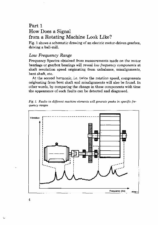
P a r t i How Does a Signal from a Rotating Machine Look Like? Fig. 1 shows a schematic drawing of an electric motor-driven gearbox, driving a ball-mill.

Low Frequency Range Frequency Spectra obtained from measurements made on the motor bearings or gearbox bearings will reveal low frequency components at shaft revolution speed originating from unbalance, misalignments, bent shaft, etc.

At the second harmonic, i.e. twice the rotation speed, components originating from bent shaft and misalignments will also be found. In other words, by comparing the change in these components with time the appearance of such faults can be detected and diagnosed.

Fig. 1. Faults in different machine elements will generate peaks in specific fre­quency ranges

4

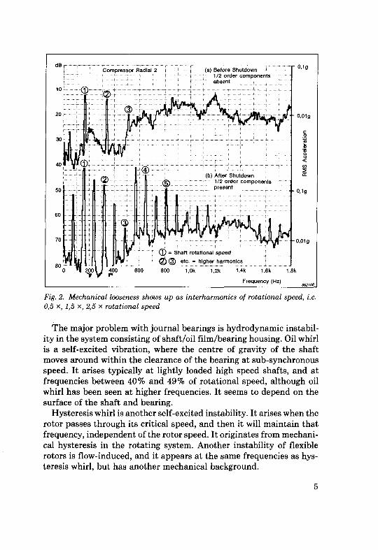
Fig. 2. Mechanical looseness shows up as interharmonics of rotational speed, i.e. 0,5 x, 1,5 x, 2,5 x rotational speed

The major problem with journal bearings is hydrodynamic instabil­ity in the system consisting of shaft/oil film/bearing housing. Oil whirl is a self-excited vibration, where the centre of gravity of the shaft moves around within the clearance of the bearing at sub-synchronous speed. It arises typically at lightly loaded high speed shafts, and at frequencies between 40% and 49% of rotational speed, although oil whirl has been seen at higher frequencies. It seems to depend on the surface of the shaft and bearing.

Hysteresis whirl is another self-excited instability. It arises when the rotor passes through its critical speed, and then it will maintain that frequency, independent of the rotor speed. It originates from mechani­cal hysteresis in the rotating system. Another instability of flexible rotors is flow-induced, and it appears at the same frequencies as hys­teresis whirl, but has another mechanical background.

5

A last type of fault appearing in this low frequency area is mechani­cal looseness. In many cases mechanical looseness will create interhar-monic and subharmonic components, i.e. a "half harmonic, a "one-and-a-half harmonic, a "two-and-a-half harmonic etc., see Fig. 2.

Medium Frequency Range Higher up in the frequency range, components originating from the toothmesh in the gearbox will be found and are in this context referred to as medium frequency components.

They will be at a frequency corresponding to rotational speed multi­plied by the number of teeth on the gear, and referred to as the toothmeshing frequency.

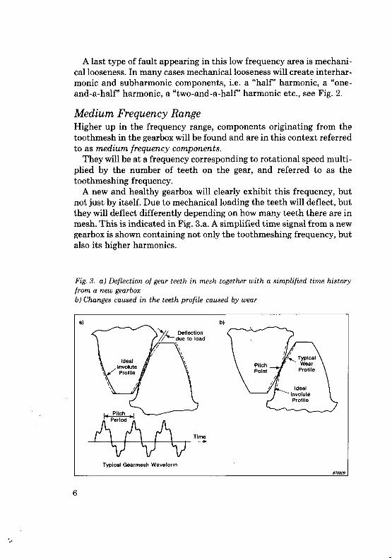
A new and healthy gearbox will clearly exhibit this frequency, but not just by itself. Due to mechanical loading the teeth will deflect, but they will deflect differently depending on how many teeth there are in mesh. This is indicated in Fig. 3.a. A simplified time signal from a new gearbox is shown containing not only the toothmeshing frequency, but also its higher harmonics.

Fig. 3. a) Deflection of gear teeth in mesh together with a simplified time history from a new gearbox b) Changes caused in the teeth profile caused by wear

6

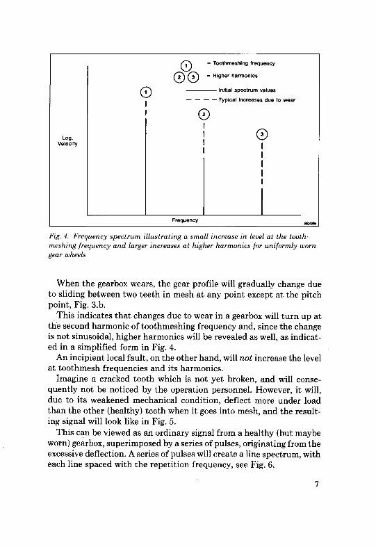
Fig. 4. Frequency spectrum illustrating a small increase in level at the tooth-meshing frequency and larger increases at higher harmonics for uniformly worn gear wheels

When the gearbox wears, the gear profile will gradually change due to sliding between two teeth in mesh at any point except at the pitch point, Fig. 3.b.

This indicates that changes due to wear in a gearbox will turn up at the second harmonic of toothmeshing frequency and, since the change is not sinusoidal, higher harmonics will be revealed as well, as indicat­ed in a simplified form in Fig. 4.

An incipient local fault, on the other hand, will not increase the level at toothmesh frequencies and its harmonics.

Imagine a cracked tooth which is not yet broken, and will conse­quently not be noticed by the operation personnel. However, it will, due to its weakened mechanical condition, deflect more under load than the other (healthy) teeth when it goes into mesh, and the result­ing signal will look like in Fig. 5.

This can be viewed as an ordinary signal from a healthy (but maybe worn) gearbox, superimposed by a series of pulses, originating from the excessive deflection. A series of pulses will create a line spectrum, with each line spaced with the repetition frequency, see Fig. 6.

7

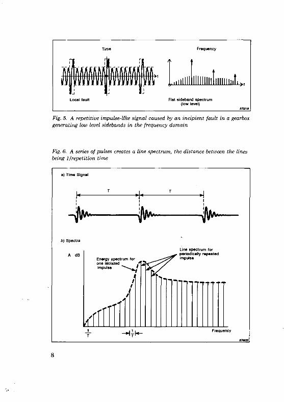
Fig. 5. A repetitive impulse-like signal caused by an incipient fault in a gearbox generating low level sidebands in the frequency domain

Fig. 6. A series of pulses creates a line spectrum, the distance between the lines being 1 /repetition time

8

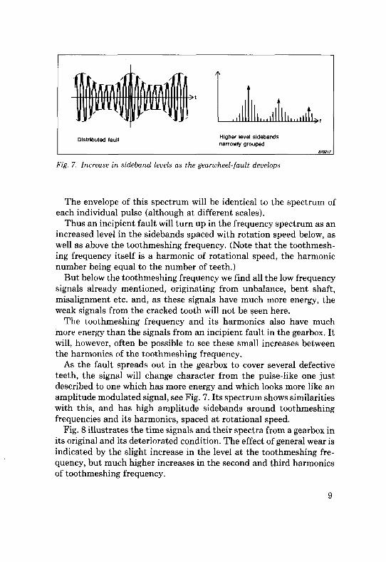
Fig. 7. Increase in sideband levels as the gearwheel-fault develops

The envelope of this spectrum will be identical to the spectrum of each individual pulse (although at different scales).

Thus an incipient fault will turn up in the frequency spectrum as an increased level in the sidebands spaced with rotation speed below, as well as above the toothmeshing frequency. (Note that the toothmesh-ing frequency itself is a harmonic of rotational speed, the harmonic number being equal to the number of teeth.)

But below the toothmeshing frequency we find all the low frequency signals already mentioned, originating from unbalance, bent shaft, misalignment etc. and, as these signals have much more energy, the weak signals from the cracked tooth will not be seen here.

The toothmeshing frequency and its harmonics also have much more energy than the signals from an incipient fault in the gearbox. It will, however, often be possible to see these small increases between the harmonics of the toothmeshing frequency.

As the fault spreads out in the gearbox to cover several defective teeth, the signal will change character from the pulse-like one just described to one which has more energy and which looks more like an amplitude modulated signal, see Fig. 7. Its spectrum shows similarities with this, and has high amplitude sidebands around toothmeshing frequencies and its harmonics, spaced at rotational speed.

Fig. 8 illustrates the time signals and their spectra from a gearbox in its original and its deteriorated condition. The effect of general wear is indicated by the slight increase in the level at the toothmeshing fre­quency, but much higher increases in the second and third harmonics of toothmeshing frequency.

9

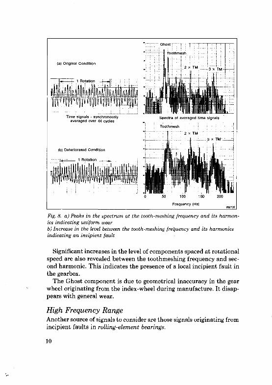
Fig. 8. a) Peaks in the spectrum at the tooth-meshing frequency and its harmon­ics indicating uniform wear b) Increase in the level between the tooth-meshing frequency and its harmonics indicating an incipient fault

Significant increases in the level of components spaced at rotational speed are also revealed between the toothmeshing frequency and sec­ond harmonic. This indicates the presence of a local incipient fault in the gearbox.

The Ghost component is due to geometrical inaccuracy in the gear wheel originating from the index-wheel during manufacture. It disap­pears with general wear.

High Frequency Range Another source of signals to consider are those signals originating from incipient faults in rolling-element bearings.

10

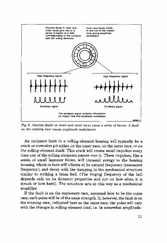
Fig. 9. Discrete faults in inner and outer races cause a series of bursts. A fault on the rotating race causes amplitude modulation

An incipient fault in a rolling-element bearing will typically be a crack or corrosion pit either on the inner race, on the outer race, or on the rolling-element itself. This crack will create small impulses every time one of the rolling-elements passes over it. These impulses, like a series of small hammer blows, will transmit energy to the bearing housing, which in turn will vibrate at its natural frequency (resonance frequency), and decay with the damping in the mechanical structure similar to striking a brass bell. (The ringing frequency of the bell depends only on its dynamic properties and not on how often it is struck or how hard). The structure acts in this way as a mechanical amplifier.

If the fault is on the stationary race, assumed here to be the outer race, each pulse will be of the same strength. If, however, the fault is on the rotating race, indicated here as the inner race, the pulse will vary with the changes in rolling-element load, i.e. be somewhat amplitude-

11

1 870231 |

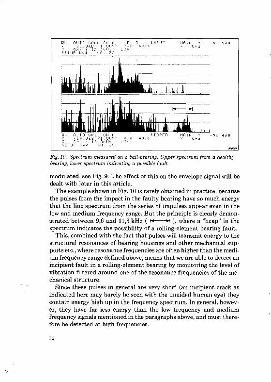
Fig. 10. Spectrum measured on a ball-bearing. Upper spectrum from a healthy bearing, lower spectrum indicating a possible fault

modulated, see Fig. 9. The effect of this on the envelope signal will be dealt with later in this article.

The example shown in Fig. 10 is rarely obtained in practice, because the pulses from the impact in the faulty bearing have so much energy that the line spectrum from the series of impulses appear even in the low and medium frequency range. But the principle is clearly demon­strated between 9,6 and 11,3 kHz ( N H ), where a "heap" in the spectrum indicates the possibility of a rolling-element bearing fault.

This, combined with the fact that pulses will transmit energy to the structural resonances of bearing housings and other mechanical sup­ports etc., where resonance frequencies are often higher than the medi­um frequency range defined above, means that we are able to detect an incipient fault in a rolling-element bearing by monitoring the level of vibration filtered around one of the resonance frequencies of the me­chanical structure.

Since these pulses in general are very short (an incipient crack as indicated here may barely be seen with the unaided human eye) they contain energy high up in the frequency spectrum. In general, howev­er, they have far less energy than the low frequency and medium frequency signals mentioned in the paragraphs above, and must there­fore be detected at high frequencies.

12

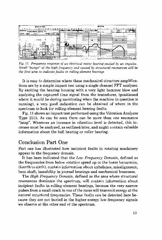
Fig. 11. Frequency response of an electrical motor bearing excited by an impulse. Small "bumps" at the high frequency end caused by structural resonances will be the first area to indicate faults in rolling-element bearings

It is easy to determine where these mechanical structure amplifica­tions are by a simple impact test using a single channel FFT analyzer. By exciting the bearing housing with a very light hammer blow and analyzing the captured time signal from the transducer, (positioned where it would be during monitoring when the machine in question is running), a very good indication can be obtained of where in the spectrum to look for rolling-element bearing faults.

Fig. 11 shows an impact test performed using the Vibration Analyzer Type 2515. As can be seen there can be more than one resonance "heap". Wherever an increase in vibration level is detected, this in­crease must be analyzed, as outlined later, and might contain valuable information about the ball bearing or roller bearing.

Conclusion Part One Part one has illustrated how incipient faults in rotating machinery appear in the frequency domain.

It has been indicated that the Low Frequency Domain, defined as the frequencies from below rotation speed up to the lower harmonics, (fourth to sixth), contain information about unbalance, misalignment, bent shaft, instability in journal bearings and mechanical looseness.

The High Frequency Domain, defined as the area where structural resonances dominate the spectrum, will contain information about incipient faults in rolling-element bearings, because the very narrow pulses from a small crack in one of the races will transmit energy at the natural structural frequencies. These faults can be detected here be­cause they are not buried in the higher-energy low-frequency signals we observe at the other end of the spectrum.

13

It has been indicated that the Medium Frequency Domain, defined as the area between the two above defined domains, will contain infor­mation about faults in gearboxes. The degree of gear wear can be seen at the toothmeshing frequency and its harmonics. However, incipient faults in a gearbox, such as a cracked tooth, not yet broken, will be seen as sidebands around the toothmeshing frequency and its harmonics, but often at far lower levels.

Part 2 Fault Detection In part one it was discussed how the vibration signal contains valuable information about the condition of rotating machines. To avoid te­dious and expensive signal analysis in day-to-day work, it is essential to use a method of detection that:

1. Detects the majority of faults as early as possible; 2. Gives as few false detections as possible; 3. Is so easy to use that even a layman can carry it out; 4. Gives enough information to make a qualified guess about the fault

to enable management to evaluate when a more thorough analysis must be made.

For many years, fault detection has been carried out by comparing RMS readings of vibration velocity with preceding readings, or with established standards, such as the German standard issued by the Institute of German Engineers VDI 2056 or the International Stan­dards ISO 2372 and 3945. The theory is that machines, of similar size and grouped after shaft power, will have similar or even the same vibration level, measured in velocity filtered from 10 Hz to 1 kHz, see Fig. 12.

As has been discussed in part one, monitoring based on this system will presumably identify unbalance, coarse misalignment and severely bent shafts because of the high energy in these signals.

As low energy signals will be buried in the more powerful vibration signals, incipient ball bearing faults or incipient gearbox faults will not be detected by this method. At least they will not be detected before they generate a vibration signal higher than the low frequency domain signals.

Fig. 14 shows how a developing fault changes the spectrum as a function of time (upper right).

14

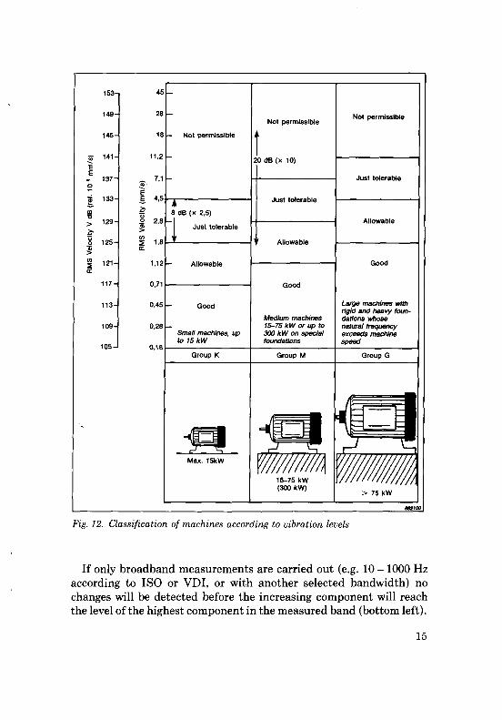
Fig. 12. Classification of machines according to vibration levels

If only broadband measurements are carried out (e.g. 10 - 1000 Hz according to ISO or VDI, or with another selected bandwidth) no changes will be detected before the increasing component will reach the level of the highest component in the measured band (bottom left).

15

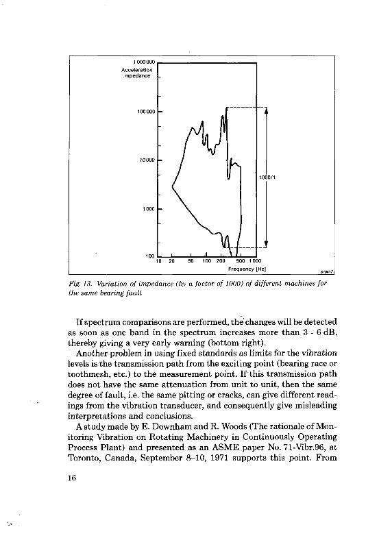
Fig. 13. Variation of impedance (by a factor of 1000) of different machines for the same bearing fault

If spectrum comparisons are performed, the'changes will be detected as soon as one band in the spectrum increases more than 3 - 6 dB, thereby giving a very early warning (bottom right).

Another problem in using fixed standards as limits for the vibration levels is the transmission path from the exciting point (bearing race or toothmesh, etc.) to the measurement point. If this transmission path does not have the same attenuation from unit to unit, then the same degree of fault, i.e. the same pitting or cracks, can give different read­ings from the vibration transducer, and consequently give misleading interpretations and conclusions.

A study made by E. Downham and R. Woods (The rationale of Mon­itoring Vibration on Rotating Machinery in Continuously Operating Process Plant) and presented as an ASME paper No. 71-Vibr.96, at Toronto, Canada, September 8-10, 1971 supports this point. From

16

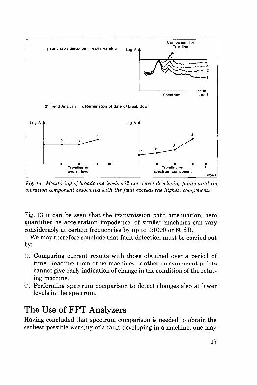
Fig. 14. Monitoring of broadband levels will not detect developing faults until the vibration component associated with the fault exceeds the highest components

Fig. 13 it can be seen that the transmission path attenuation, here quantified as acceleration impedance, of similar machines can vary considerably at certain frequencies by up to 1:1000 or 60 dB.

We may therefore conclude that fault detection must be carried out by:

O. Comparing current results with those obtained over a period of time. Readings from other machines or other measurement points cannot give early indication of change in the condition of the rotat­ing machine.

O. Performing spectrum comparison to detect changes also at lower levels in the spectrum.

The Use of FFT Analyzers Having concluded that spectrum comparison is needed to obtain the earliest possible warning of a fault developing in a machine, one may

17

V

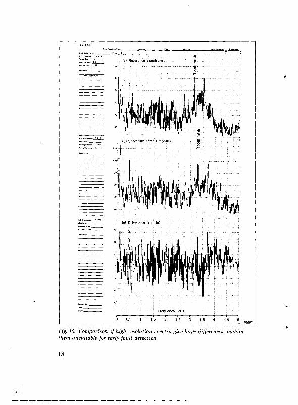
Fig. 15. Comparison of high resolution spectra give large differences, making them unsuitable for early fault detection

18

be tempted to use the storage and comparison capability of most single channel analyzers. However, as shown below, problems can be envisaged.

Very small changes in speed will shift the position of the peaks and result in large differences and give false exceedances, and therefore false warnings see Fig. 15.

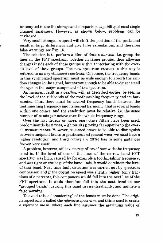
The solution is to perform a kind of data reduction, i.e. group the lines in the FFT spectrum together in larger groups, thus allowing changes inside each of these groups without interfering with the over­all level of these groups. The new spectrum created in this way is referred to as a synthesized spectrum. Of course, the frequency bands in this synthesized spectrum must be wide enough to absorb the ran­dom changes in the signal, but narrow enough to be able to detect small changes in the major component of the spectrum.

An incipient fault in a gearbox will, as described earlier, be seen in the level of the sidebands of the toothmeshing frequency and its har­monics. Thus there must be several frequency bands between the toothmeshing frequency and its second harmonic, that is several bands within one octave, and the resolution must be relative, i.e. the same number of bands per octave over the whole frequency range.

Over the last decade or more, one-octave filters have been used, predominantly by navies, with results proving far superior to the over­all measurements. However, as stated above to be able to distinguish between incipient faults in gearboxes and general wear, we must have a higher resolution, and third octave (s» 23%) has in some instances proven very useful.

A problem, however, still exists regardless of how wide the frequency band is. If the level of one of the lines of the narrow band FFT spectrum was high, caused by for example a toothmeshing frequency, and was right on the edge of the band limit, it would dominate the level of that band. Next time fault detection was carried out by spectrum comparison and if the operation speed was slightly higher, (only frac­tions of a percent), this component would fall into the next line of the FFT spectrum. It could therefore fall into the next band in our "grouped bands", causing this band to rise drastically, and indicate a false warning.

To avoid this, a "broadening" of the bands must be done. The origi­nal spectrum is called the reference spectrum, and this is used to create a reference mask, where each line assumes the maximum value of

19

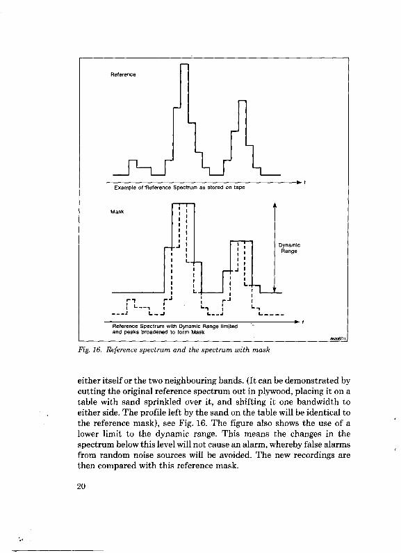
Fig. 16. Reference spectrum and the spectrum with mask

either itself or the two neighbouring bands. (It can be demonstrated by cutting the original reference spectrum out in plywood, placing it on a table with sand sprinkled over it, and shifting it one bandwidth to either side. The profile left by the sand on the table will be identical to the reference mask), see Fig. 16. The figure also shows the use of a lower limit to the dynamic range. This means the changes in the spectrum below this level will not cause an alarm, whereby false alarms from random noise sources will be avoided. The new recordings are then compared with this reference mask.

20

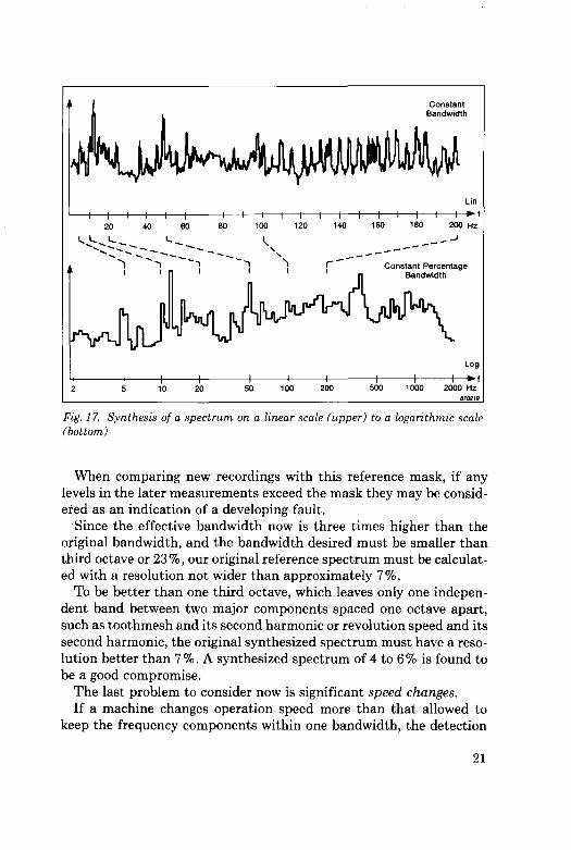
Fig. 17. Synthesis of a spectrum on a linear scale (upper) to a logarithmic scale (bottom)

When comparing new recordings with this reference mask, if any levels in the later measurements exceed the mask they may be consid­ered as an indication of a developing fault.

Since the effective bandwidth now is three times higher than the original bandwidth, and the bandwidth desired must be smaller than third octave or 23%, our original reference spectrum must be calculat­ed with a resolution not wider than approximately 7%.

To be better than one third octave, which leaves only one indepen­dent band between two major components spaced one octave apart, such as toothmesh and its second harmonic or revolution speed and its second harmonic, the original synthesized spectrum must have a reso­lution better than 7%. A synthesized spectrum of 4 to 6% is found to be a good compromise.

The last problem to consider now is significant speed changes. If a machine changes operation speed more than that allowed to

keep the frequency components within one bandwidth, the detection

21

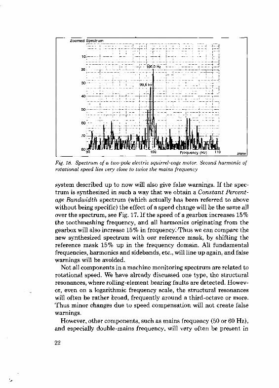
Fig. 18. Spectrum of a two-pole electric squirrel-cage motor. Second harmonic of rotational speed lies very close to twice the mains frequency

system described up to now will also give false warnings. If the spec­trum is synthesized in such a way that we obtain a Constant Percent­age Bandwidth spectrum (which actually has been referred to above without being specific) the effect of a speed change will be the same all over the spectrum, see Fig. 17. If the speed of a gearbox increases 15 % the toothmeshing frequency, and all harmonics originating from the gearbox will also increase 15% in frequency.-Thus we can compare the new synthesized spectrum with our reference mask, by shifting the reference mask 15% up in the frequency domain. All fundamental frequencies, harmonics and sidebands, etc., will line up again, and false warnings will be avoided.

Not all components in a machine monitoring spectrum are related to rotational speed. We have already discussed one type, the structural resonances, where rolling-element bearing faults are detected. Howev­er, even on a logarithmic frequency scale, the structural resonances will often be rather broad, frequently around a third-octave or more. Thus minor changes due to speed compensation will not create false warnings.

However, other components, such as mains frequency (50 or 60 Hz), and especially double-mains frequency, will very often be present in

22

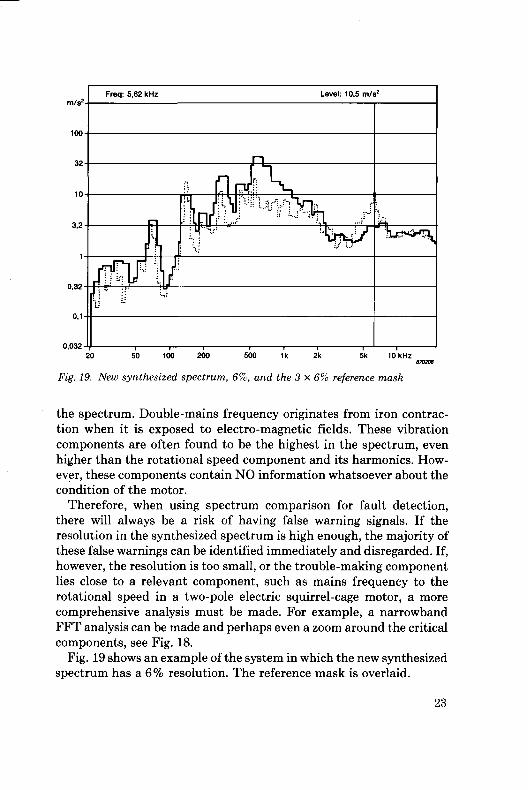
Fig. 19. New synthesized spectrum, 6%, and the 3 x 6% reference mask

the spectrum. Double-mains frequency originates from iron contrac­tion when it is exposed to electro-magnetic fields. These vibration components are often found to be the highest in the spectrum, even higher than the rotational speed component and its harmonics. How­ever, these components contain NO information whatsoever about the condition of the motor.

Therefore, when using spectrum comparison for fault detection, there will always be a risk of having false warning signals. If the resolution in the synthesized spectrum is high enough, the majority of these false warnings can be identified immediately and disregarded. If, however, the resolution is too small, or the trouble-making component lies close to a relevant component, such as mains frequency to the rotational speed in a two-pole electric squirrel-cage motor, a more comprehensive analysis must be made. For example, a narrowband FFT analysis can be made and perhaps even a zoom around the critical components, see Fig. 18.

Fig. 19 shows an example of the system in which the new synthesized spectrum has a 6% resolution. The reference mask is overlaid.

23

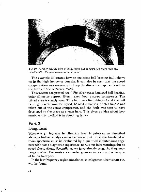
Fig. 20. A roller bearing with a fault, taken out of operation more than five months after the first indication of a fault

The example illustrates how an incipient ball-bearing fault shows up in the high-frequency domain. It can also be seen that the speed compensation was necessary to keep the discrete components within the limits of the reference mask.

This system has proved itself. Fig. 20 shows a damaged ball bearing, outer diameter approx. 30 cm, taken from a screw compressor. The pitted area is clearly seen. This fault was first detected and the ball bearing then ran uninterrupted the next 5 months. At this time it was taken out of the screw compressor, and the fault was seen to have developed to the stage as shown here. This gives an idea about how sensitive this method is in detecting faults:

Part 3 Diagnosis Whenever an increase in vibration level is detected, as described above, a further analysis must be carried out. First the baseband or zoom spectrum must be evaluated by a qualified maintenance engi­neer with some diagnostic experience, to rule out false warnings due to speed fluctuations. Secondly, as we have already seen, the frequency range in which the levels are exceeded gives an indication of what type of faults to expect.

In the low frequency region unbalance, misalignment, bent shaft etc. will be found.

24

In the medium frequency region, indication of wear and incipient faults in a gearbox will be found, as well as eccentricity, uneven gear­wheels, misaligned gearwheels, etc. In the high frequency region, infor­mation about incipient faults in rolling-element bearings, or any other phenomenon giving a train of narrow sharp pulses, will be detected.

Based on the above discussion, one or more of the following methods may be selected for further diagnostic analysis.

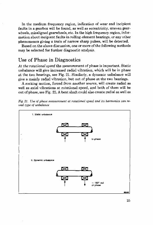
Use of Phase in Diagnostics At the rotational speed the measurement of phase is important. Static unbalance will give increased radial vibration, which will be in phase at the two bearings, see Fig. 21. Similarly, a dynamic unbalance will give a mainly radial vibration, but out of phase at the two bearings.

A rocking motion, forced from another source, will create radial as well as axial vibrations at rotational speed, and both of them will be out of phase, see Fig. 22. A bent shaft could also create radial as well as

Fig. 21. Use of phase measurement at rotational speed and its harmonics can re­veal type of unbalance

25

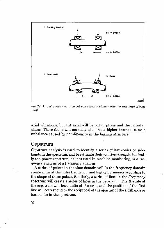
Fig. 22. Use of phase measurement can reveal rocking motion or existence of bent shaft

axial vibrations, but the axial will be out of phase and the radial in phase. These faults will normally also create higher harmonics, even unbalance caused by non-linearity in the bearing structure.

Cepstrum Cepstrum analysis is used to identify a series of harmonics or side­bands in the spectrum, and to estimate their relative strength. Basical­ly the power cepstrum, as it is used in machine monitoring, is a fre­quency analysis of a frequency analysis.

A series of pulses in the time domain will in the frequency domain create a line at the pulse frequency, and higher harmonics according to the shape of these pulses. Similarly, a series of lines in the Frequency spectrum will create a series of lines in the Cepstrum. The X-scale of the cepstrum will have units of l/Rz or s., and the position of the first line will correspond to the reciprocal of the spacing of the sidebands or harmonics in the spectrum.

26

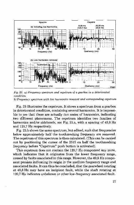
Fig. 23. a) Frequency spectrum and cepstrum of a gearbox in a deteriorated condition b) Frequency spectrum with low harmonics removed and corresponding cepstrum

Fig. 23 illustrates the cepstrum. It shows a spectrum from a gearbox in deteriorated condition, containing several harmonics. It is impossi­ble to see that there are actually two series of harmonics, indicating two different phenomena. The cepstrum identifies two families of harmonics and/or sidebands, see Fig. 23.a, with a spacing of 49,8 Hz and 120,7 Hz respectively.

Fig. 23.b shows the same spectrum, but edited, such that frequencies below approximately half the toothmeshing frequency are removed. The cepstrum of this spectrum is then calculated. (This can be carried out by positioning the cursor of the 2515 on half the toothmeshing frequency before "Cepstrum" push button is activated).

This cepstrum does not contain the 120,7 Hz component any more, which indicates that it originates from the lower frequency range, caused by faults associated in this range. However, the 49,8 Hz compo­nent persists indicating its origin in the medium frequency range and associated faults. It can thus be concluded, that the gearwheel rotating at 49,8 Hz may have an incipient fault, while the shaft rotating at 120,7 Hz indicates unbalance or other low-frequency associated fault.

27

Finally, cepstrum is to a high degree insensitive to phase differences in the original signal, and to the influence from the transmission path, e.g. cepstra of measurements on a gearbox at two different bearings will be nearly identical.

Envelope Detection It has been shown that an incipient fault in a rolling-element bearing will create a series of sharp pulses, but pulses with very little energy content, see Fig. 9. These faults are detected by monitoring the in­crease in vibration level at structural resonances, but the analysis needed to establish that it is a faulty bearing, and not a signal originat­ing from for example a forced lubrication system or another spiky signal, cannot be made by a simple FFT analyzer.

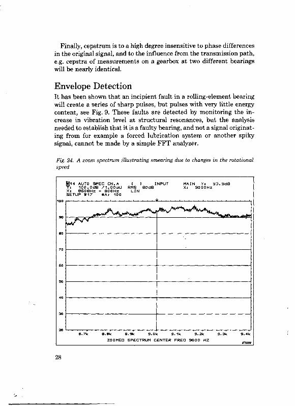
Fig. 24. A zoom spectrum illustrating smearing due to changes in the rotational speed

28

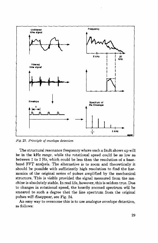
.Fig. 25. Principle of envelope detection

The structural resonance frequency where such a fault shows up will be in the kHz range, while the rotational speed could be as low as between 1 to 2 Hz, which could be less than the resolution of a base­band FFT analysis. The alternative is to zoom and theoretically it should be possible with sufficiently high resolution to find the har­monics of the original series of pulses amplified by the mechanical structure. This is viable provided the signal measured from the ma­chine is absolutely stable. In real life, however, this is seldom true. Due to changes in rotational speed, the heavily zoomed spectrum will be smeared to such a degree that the line spectrum from the original pulses will disappear, see Fig. 24.

An easy way to overcome this is to use analogue envelope detection, as follows:

29

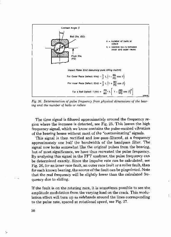
Fig. 26. Determination of pulse frequency from physical dimensions of the bear­ing and the number of balls or rollers

The time signal is filtered approximately around the frequency re­gion where the increase is detected, see Fig. 25. This leaves the high frequency signal, which we know contains the pulse-excited vibration of the bearing house without most of the "contaminating" signals.

This signal is then rectified and low-pass-filtered, at a frequency approximately one half the bandwidth of the bandpass filter. The signal now looks somewhat like the original pulses from the bearing, but of most significance, we have thus recreated the pulse frequency. By analysing this signal in the FFT analyzer, the pulse frequency can be determined exactly. Since the impulse rate can be calculated, see Fig. 26, for an inner race fault, an outer race fault or a roller fault, then for each known bearing, the source of the fault can be pinpointed. Note that the real frequency will be slightly lower than the calculated fre­quency due to sliding.

If the fault is on the rotating race, it is sometimes possible to see the amplitude modulation from the varying load on the crack. This modu­lation effect will turn up as sidebands around the lines corresponding to the pulse rate, spaced at rotational speed, see Fig. 27.

30

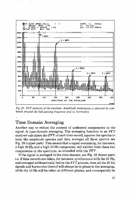
Fig. 27. FFT analysis of the envelope. Amplitude modulation is detected by side­bands around the ball passing frequency and its harmonics

Time Domain Averaging Another way to reduce the content of undesired components in the signal, is time-domain averaging. The averaging function in an FFT analyzer calculates the FFT of each time record, squares the spectra to form the amplitude spectra and then averages all these spectra see Fig. 28 (upper part). This means that a signal containing, for instance, a high 20 Hz and a high 33 Hz component, will exhibit both these two components in the spectrum, as intended with the FFT.

If the signal is averaged in the time domain, see Fig. 28 (lower part) i.e. if time records are taken, for instance, synchronous with the 20 Hz, and averaged arithmetically before the FFT process, then all the 20 Hz signals and harmonics thereof will always be in phase in the averaging, while the 33 Hz will be taken at different phases, and consequently be

31

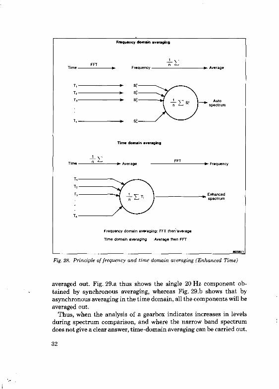
Fig. 28. Principle of frequency and time domain averaging (Enhanced Time)

averaged out. Fig. 29.a thus shows the single 20 Hz component ob­tained by synchronous averaging, whereas Fig. 29.b shows that by asynchronous averaging in the time domain, all the components will be averaged out.

Thus, when the analysis of a gearbox indicates increases in levels during spectrum comparison, and where the narrow band spectrum :

does not give a clear answer, time-domain averaging can be carried out.

32

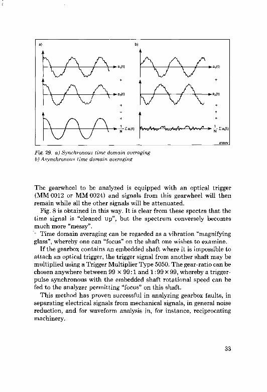
Fig. 29. a) Synchronous time domain averaging b) Asynchronous time domain averaging

The gearwheel to be analyzed is equipped with an optical trigger (MM 0012 or MM 0024) and signals from this gearwheel will then remain while all the other signals will be attenuated.

Fig. 8 is obtained in this way. It is clear from these spectra that the time signal is "cleaned up", but the spectrum conversely becomes much more "messy". '■■ Time domain averaging can be regarded as a vibration "magnifying glass", whereby one can "focus" on the shaft one wishes to examine.

If the gearbox contains an embedded shaft where it is impossible to attach an optical trigger, the trigger signal from another shaft may be multiplied using a Trigger Multiplier Type 5050. The gear-ratio can be chosen anywhere between 99 x 99:1 and 1:99 x 99, whereby a trigger-pulse synchronous with the embedded shaft rotational speed can be fed to the analyzer permitting "focus" on this shaft.

This method has proven successful in analyzing gearbox faults, in separating electrical signals from mechanical signals, in general noise reduction, and for waveform analysis in, for instance, reciprocating machinery.

33

Part 4 Trending Fault Developments The trending technique is frequently used in monitoring, quite often simply to monitor a development such as oil pressure or cooling water temperature. In the case of vibration monitoring, however, it is a little more complicated. Ordinary day-to-day monitoring with no fault de­velopments will give a series of spectra with "no significant changes". An incipient fault will cause a line og group of lines to suddenly increase. Then, as the fault slowly spreads out, the vibration level will gradually rise. This would be the case with an incipient rolling-ele­ment bearing fault, or the effect of ordinary wear. However, the ap­pearance of oil-whirl in journal bearings will also give rise to an in­crease in the spectrum, but this will not necessarily develop gradually. It will not, therefore, give an indication of a slowly deteriorating condi­tion, with an anticipated remaining safe operating time. Loss of small blades in a turbine will also be detected, but the change in the spec­trum will not "develop" until the next blade is lost.

However, if the detection of a fault leads to a proper diagnosis, from which it can be assumed that the fault will develop gradually, and hence the vibration signal will develop gradually in parallel and not stepwise, then, and only then, trending can be carried out. The fre­quency range for the trend analysis should be chosen on the frequency bands where increases are detected to give a good indication of the fault development and to determine the remaining safe operating time.

This type of trending can be done with the computer which already handles the spectrum comparison. If the spectra which exceed the prescribed levels are stored together with the reference spectra, a trending program included in the software would only need to have the information of how high an increase in level the maintenance engineer is willing to accept. Fig. 30 gives an example of a trending program included in the Monitoring Software WT 9114. It is also an example of a trending which is doubtful. The fault does not seem to develop "gradually" and the estimated lead-time of 7 months is not reliable.

If information from earlier experience is available, this should natu­rally be used, but if not, the old overall-level standards will give a fairly good indication. They indicate that an increase in vibration of 2,5 times, or 8 dB, warrants a further analysis, and an increase of 10 times, or 20 dB, demands immediate action. These values are, however, con-

34

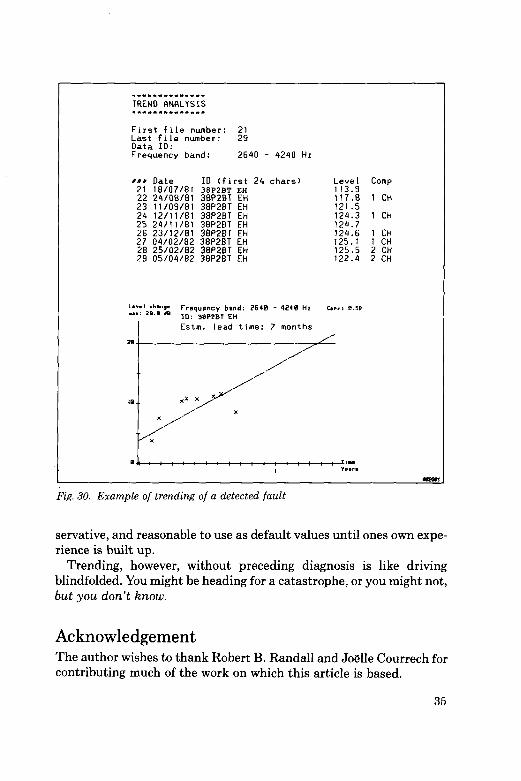
Fig. 30. Example of trending of a detected fault

servative, and reasonable to use as default values until ones own expe­rience is built up.

Trending, however, without preceding diagnosis is like driving blindfolded. You might be heading for a catastrophe, or you might not, but you don't know.

Acknowledgement The author wishes to thank Robert B. Randall and Joelle Courrech for contributing much of the work on which this article is based.

35

References [1] "Machine Health Monitoring". Brilel & Kjaer

Publication [2] Harris, H.M. & "Shock and Vibration Handbook" McGraw-Hill

Crede, C.E. Book Company [3] Randall, R.B. "Frequency Analysis". Briiel & Kjaer Publication [4] Mitchell, J.S. "Machinery Analysis and Monitoring". Penn-

Well Publishing Company, Tulsa, Oklahoma, USA

[5] Bloch, H.P. & "Practical Management for Process Plants: Geitner, F.P. Vol.1: Improving machinery reliability,

Vol.2: Machinery failure Analysis and troubleshooting, Vol.3: Machinery component Maintenance and repair, Vol.4: Major process equipment Maintenance and repair

36

Previously issued numbers of Briiel & Kjaer Technical Review (Continued from cover page 2) 2-1982 Thermal Comfort 1-1982 Human Body Vibration Exposure and its Measurement. 4-1981 Low Frequency Calibration of Acoustical Measurement Systems.

Calibration and Standards. Vibration and Shock Measurements. 3-1981 Cepstrum Analysis. 2-1981 Acoustic Emission Source Location in Theory and in Practice. 1-1981 The Fundamentals of Industrial Balancing Machines and Their

Applications. 4-1980 Selection and Use of Microphones for Engine and Aircraft Noise

Measurements. 3-1980 Power Based Measurements of Sound Insulation.

Acoustical Measurement of Auditory Tube Opening. 2-1980 Zoom-FFT. 1-1980 Luminance Contrast Measurement. 4-1979 Prepolarized Condenser Microphones for Measurement Purposes.

Impulse Analysis using a Real-Time Digital Filter Analyzer. 3-1979 The Rationale of Dynamic Balancing by Vibration Measurements.

Interfacing Level Recorder Type 2306 to a Digital Computer. 2-1979 Acoustic Emission. 1-1979 The Discrete Fourier Transform and FFT Analyzers. 4-1978 Reverberation Process at Low Frequencies. 3-1978 The Enigma of Sound Power Measurements at Low Frequencies.

Special technical literature Briiel & Kjaer publishes a variety of technical literature which can be ob­tained from your local Briiel & Kjaer representative. The following literature is presently available:

O Mechanical Vibration and Shock Measurements (English), 2nd edition O Modal Analysis of Large Structures-Multiple Exciter Systems (English) O Acoustic Noise Measurements (English), 3rd edition O Architectural Acoustics (English) O Noise Control (English, French) O Frequency Analysis (English) O Electroacoustic Measurements (English, German, French, Spanish) O Catalogues (several languages) O Product Data Sheets (English, German, French, Russian) Furthermore, back copies of the Technical Review can be supplied as shown in the list above. Older issues may be obtained provided they are still in stock.