Cepstrum Analysis and Gearbox Fault Diagnosis

233—80

Cepstrum Analysis and Gearbox Fault Diagnosis Edition 2*

by R.B. Randall, B. Tech., B.A. Bruel & Kjaer

1. Introduction

The cepstrum is defined in a num­ber of different ways, but all can be considered as a spectrum of a logar­ithmic spectrum (i.e. logarithmic am­plitude, but linear frequency scale). This means that cepstrum analysis can be used as a tool for the detec­tion of periodicity in a spectrum, for example families of harmonics with uniform spacing. The logarithmic amplitude scale emphasizes the har­monic structure of the spectrum and reduces the influence of the somewhat random transmission path by which the signal travels from the source to the measure­ment point.

One of the earliest applications of the cepstrum was in speech analy­sis, with the aim of detecting the harmonic structure of voiced sounds and measuring voice pitch (Refs.1, 2). Another was in the study of signals containing echoes, which also give a periodic structure to the spectrum (Refs. 1, 3).

The type of periodic structure con­sidered here, however, is given by the families of sidebands commonly found in gearbox vibration spectra, and which often are an indication of faults of various kinds. Several peo­ple have shown that such side­bands can be considered to arise

* Replaces Application Note No. 1 3—1 50 from 1973.

Fig.1. Amplitude modulation of toothmesh _ , . , , . . , «;«»ai H..o+«o^««*r:^t„ The former effect shows up as side-signal due to eccentricity r

bands around the toothmeshing fre­quency and its harmonics, while

from modulation of the otherwise the latter tends to be limited to fre-uniform toothmeshing vibrations by quencies lower than the toothmesh-lower frequencies, typically the ing frequency. shaft rotational speeds (Refs.4—7). Eccentricity of one gearwheel, for Even for gearboxes in good condi-example, would tend to give an am- t ion, the spectra normally contain plitude modulation of the basic vi- such sidebands but at a level which bration generated at the toothmesh- remains constant wi th t ime. ing frequency (and its harmonics) Changes in the number and wi th an envelope period correspond- strength of the sidebands would ing to the shaft rotation (Fig.1). At generally indicate a deterioration in the same t ime, the variations in condition. tooth contact pressure, which give the amplitude modulation, give rise The spacing of these sidebands to rotational speed fluctuations thus contains very valuable informa-which cause frequency modulation tion as to the source of a vibration at the same frequency. Thus, ampli- problem, often tracing it to a particu-tude or frequency modulation sel- lar gear in a complicated gearbox, dom occurs in isolation, but on the or in the case of load fluctuations other hand both give rise to a family (for example at the lobe-meshing of sidebands with the same spacing frequency of a blower) establishing (the fundamental modulating fre- that the source of the modulation quency) and it is this sideband spac- lies outside the gearbox itself. Of-ing which contains the basic diag- ten, however, as soon as there is nostic information as to the source more than one family of sidebands of the modulation. present at the one time, it can be

1

Appendix A contains a more de­tailed discussion of the generation of vibrations in gearboxes, and shows how uniformly distributed faults (i.e. the same for each tooth) only affect the toothmeshing har­monics, while more localised ef­fects can be interpreted as combina­tions of amplitude and frequency modulation and additive impulses. The former effect shows up as side­bands around the toothmeshing fre­quency and its harmonics, while

difficult to distinguish them by eye, the spectral information. The cep- and easing the problem of monitor-and this is where the cepstrum is strum may also be useful as a data ing changes in condition. useful in separating the various peri- reduction technique, effectively red-odicities. Here it can be considered ucing a whole pattern of sidebands as a diagnostic aid in interpreting into a single line in the cepstrum,

2. The Cepstrum

The cepstrum was originally de- discussion of the relationships be- spectrum. This is in fact virtually fined (Ref.3) as the "power spec- tween the various forms of the cep- the same as a rectified version (mod-trum of the logarithm of the power strum, and many of their applica- ulus) of Eqn.(3), since for a real, spectrum", or mathematically: tions. even function such as a power spec­

trum, the forward and inverse trans-C(r) = .¥\ log Fxx(f)} 2 (1) Note that the independent vari- forms give the same result except

able, r, of the cepstrum has the di- for a possible scaling factor. where Fxx(f) is the power spectrum mensions of t ime, but is known as of the time signal fx(t) "quefrency". This is a useful termi- The above discussion applies to

nology for those used to interpret- the case where the 2-sided repres-i.e. Fxx(f) = J^{ f x ( t ) } 2 (2) ing time signals in terms of their fre- entation of the power spectrum (i.e.

quency content, since a "high quef- including both positive and negative and J*7 { } represents the forward rency" represents rapid fluctuations frequencies) is used. Fourier theory Fourier Transform of the bracketed in the spectrum (small frequency (see, for example. Appendix B) quantity. Later, a newer definition spacings) and a " low quefrency" re- shows that for such a real, even was coined as the "inverse trans- presents slow changes with fre- function the Fourier transform is form of the logarithm of the power quency (large frequency spacings). also a real, even function and thus spectrum", or Where peaks in the cepstrum result the cepstrum is represented by the

from families of sidebands, the quef- real parts of the transform. If, on C(r) ^ - 1 { ' c x j F x x ( f } } (3)

rency of the peak represents the pe- the other hand, the one-sided spec-riodic time of the modulation, and trum is transformed (i.e. the nega-

One of the reasons for using this its reciprocal the modulation fre- tive frequency components are set definition is that it highlights the quency. Note that the quefrency to zero) the real parts wi l l still be ef-connection between the cepstrum says nothing about absolute fre- fectively the same (and this thus and the autocorrelation function, quency, only about frequency spac- provides an efficient way of achiev-which can be obtained as the in- ings. ing the same result) but the imagi-verse transform of the power spec- nary parts wi l l represent the Hilbert t rum, i.e. In the application considered transform of the real parts. The cep-

here, viz. the detection of peaks re- strum obtained by squaring and ad-R | r j = j ^ _ i j p (fj j (4) presenting strong periodicity in the ding the real and imaginary parts at

(logarithmic) spectrum, the choice each quefrency and extracting the of definition (1) or (3) is not so crit i- square root wi l l hereinafter be re-

The definition (3) is also closer to cal, as both wil l show distinct peaks ferred to as the "amplitude cep-that of the "complex cepstrum" in the same location. The squaring strum (of the one-sided spectrum)". (Ref.1) which is the "inverse trans- of Eqn.(1) tends to emphasize the As wil l later be shown by an exam-form of the complex logarithm of largest peaks, which is not always pie, this is a very useful form when the complex spectrum" and in fact an advantage, and in fact the au- the spectrum being analyzed is ob­is identical to it for spectra wi th thor has often adopted a further def- tained by a "zoom" process. Appen-zero phase. The complex cepstrum init ion, represented by the square dix B includes a discussion of the

r

is not further discussed here, how- root of Eqn.(1), viz. the amplitude theoretical background. ever. Ref.1 contains an excellent spectrum rather than the power

2 . 1 . The cepstrum vs. the autocorrelation function In comparison wi th the autocorre- (3) and (4)) and it is here that the bration) signal at an external meas-

lation function, the logarithms of main advantage of the cepstrum urement point is the product of the the spectrum values are taken be- lies. Consider the normal case power spectrum of the source func-fore inverse transformation (Eqns. where the power spectrum of a (vi- tion and (the squared amplitude of)

2

Fig.2. Lack of sensitivity of cepstrum to transmission path effects

3

the frequency response function of and the additive relationship is the cepstrum. Since they often have the transmission path, i.e. maintained by the linear Fourier quite different quefrency contents,

transform, i.e. they will then also be separated in Fyy(f) = FX X (T) H x y ( f ) (5) t n e cepstrum, and under those con-

j * r _ i j l o q p J = rj\ ditions additive even using Eqn.(1), The effect of taking the logarithm is since cross terms vanish. By con-to transform the multiplication to an . j ^ - i j i oqF I + J ^ - i i 2 l o q H } trast, the autocorrelation obtained addition, i.e. x x x v by inverse transformation of Eqn.(5)

involves a convolution of the two ef-log F = log Fxx + 2 log Hxy (6) meaning that source and trans- fects, which is much more compli-

mission path effects are additive in cated.

3. Advantages of Cepstrum vs. Spectrum Analysis

The cepstrum can be considered spectrum and is much less likely to gearbox, are the phase relation-as an aid to the interpretation of the be affected. Fig.2 illustrates a typi- ships of amplitude and frequency spectrum, in particular with respect cal case with spectra taken from modulation at the same frequency. to sideband families, because it two separate measurement points Even though they are coupled at the presents the information in a more on the same gearbox, but represen- source, the frequency modulation is efficient manner. One advantage re- ting the same internal condition. most directly related to the torsional suiting directly from the considera- The spectra are quite different in properties of the system, while the tions of the previous paragraph is shape (for example at 2,6 kHz there amplitude modulation is more af-the lack of sensitivity to trans- is a peak in one spectrum and a fected by the lateral response pro-mission path effects. Small changes trough in the other) but the signifi- perties, and this can explain phase in positioning of an accelerometer, cant cepstrum components are al- shifts. Either amplitude or fre-for example, can modify the overall most identical. The different spec- quency modulation in isolation shape of the spectrum and thus in- trum shapes show up in the "low tends to give symmetrical families fluence the level of individual side- quefrency" range of the cepstra. of sidebands around the carrier fre-bands. The cepstrum component quency, but the combination will us-corresponding to a given sideband Another effect which can modify ually give reinforcement on one spacing, however, is an average the shape of the spectrum, even side and cancellation on the other, sideband height over the whole with the same degree of fault in the which thus partly explains the non-

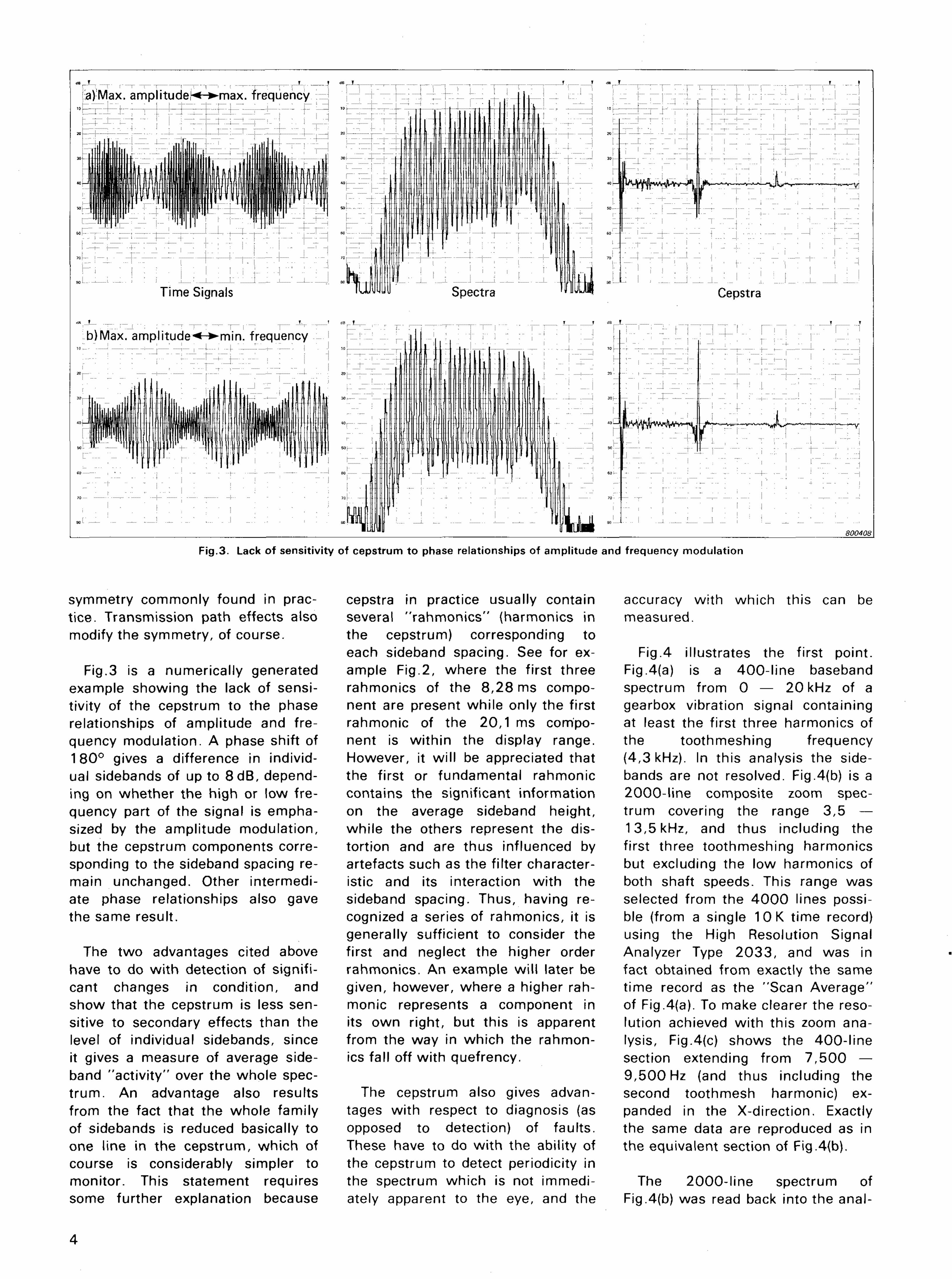
Fig.3. Lack of sensitivity of cepstrum to phase relationships of amplitude and frequency modulation

symmetry commonly found in prac- cepstra in practice usually contain accuracy with which this can be tice. Transmission path effects also several "rahmonics" (harmonics in measured. modify the symmetry, of course. the cepstrum) corresponding to

each sideband spacing. See for ex- Fig.4 illustrates the first point. Fig.3 is a numerically generated ample Fig.2, where the first three Fig.4(a) is a 400-l ine baseband

example showing the lack of sensi- rahmonics of the 8,28 ms compo- spectrum from 0 — 20 kHz of a tivity of the cepstrum to the phase nent are present while only the first gearbox vibration signal containing relationships of amplitude and fre- rahmonic of the 20,1 ms compo- at least the first three harmonics of quency modulation. A phase shift of nent is within the display range. the toothmeshing frequency 180° gives a difference in individ- However, it wi l l be appreciated that (4,3 kHz). In this analysis the side-ual sidebands of up to 8 d B , depend- the first or fundamental rahmonic bands are not resolved. Fig.4(b) is a ing on whether the high or low fre- contains the significant information 2000- l ine composite zoom spec-quency part of the signal is empha- on the average sideband height, trum covering the range 3,5 — sized by the amplitude modulation, whi le the others represent the dis- 13,5 kHz, and thus including the but the cepstrum components corre- tortion and are thus influenced by first three toothmeshing harmonics sponding to the sideband spacing re- artefacts such as the filter character- but excluding the low harmonics of main unchanged. Other intermedi- istic and its interaction wi th the both shaft speeds. This range was ate phase relationships also gave sideband spacing. Thus, having re- selected from the 4 0 0 0 lines possi-the same result. cognized a series of rahmonics, it is ble (from a single 10 K time record)

generally sufficient to consider the using the High Resolution Signal The two advantages cited above first and neglect the higher order Analyzer Type 2033 , and was in

have to do wi th detection of signifi- rahmonics. An example wi l l later be fact obtained from exactly the same cant changes in condition, and given, however, where a higher rah- time record as the "Scan Average" show that the cepstrum is less sen- monic represents a component in of Fig.4(a). To make clearer the reso-sitive to secondary effects than the its own right, but this is apparent lution achieved with this zoom ana-level of individual sidebands, since from the way in which the rahmon- lysis, Fig.4(c) shows the 400-l ine it gives a measure of average side- ics fall off with quefrency. section extending from 7,500 — band "activity" over the whole spec- 9 ,500 Hz (and thus including the t rum. An advantage also results The cepstrum also gives advan- second toothmesh harmonic) ex-from the fact that the whole family tages with respect to diagnosis (as panded in the X-direction. Exactly of sidebands is reduced basically to opposed to detection) of faults. the same data are reproduced as in one line in the cepstrum, which of These have to do wi th the ability of the equivalent section of Fig.4(b). course is considerably simpler to the cepstrum to detect periodicity in monitor. This statement requires the spectrum which is not immedi- The 2000- l ine spectrum of some further explanation because ately apparent to the eye, and the Fig.4(b) was read back into the anal-

4

Fig.4. (a) 400-l ine baseband spectrum (b) 2000- l ine composite zoom spectrum (c) 400-l ine zoom spectrum f rom b) (d) Cepstrum of 2000-t ine spectrum b) (average of 5)

yzer digitally as a time signal (using ponents are rahmonics of one of more accurately in the spectrum. In an HP 9825 calculator) and then a the two shaft speeds. This periodic- the cepstrum, the corresponding "scan" analysis performed to obtain ity is not so apparent to the eye in quefrency is 95,9 ms (10,4 Hz) the cepstrum corresponding to the the zoom spectra, since the mixture while there is also a series of rah-entire spectrum. (If it had contained of the two periodicities gives a monies corresponding to the input significant information, the entire "quasi-periodic" structure. shaft speed (28,1 ms — 35,6 Hz). 4000- l ine spectrum could have With that input speed, the output been read back into the 10K me- The second diagnostic advantage shaft speed would have been mory of the Analyzer Type 2033). is illustrated by Fig.5. This shows 5,4 Hz, and it was first suspected This thus represents the "amplitude spectra and cepstra for two truck that the modulating frequency was cepstrum of the one-sided spec- gearboxes, in good and bad condi- its second harmonic. However, that t r um" , and is reproduced as Fig.4(d) tion respectively, running on a test would have been 10,8 Hz, not (actually Fig.4(d) is the average of 5 stand with first gear engaged. The 10,4 Hz, and in the end it was such cepstra). The cepstrum shows good gearbox shows no marked found that the latter corresponded that only two components, corre- spectrum periodicity, but the spec- exactly to second gear speed, indi-sponding to the two shaft speeds trum of the bad one contains a eating that this was the modulation 85 Hz and 50 Hz, are important large number of sidebands wi th a source, even though first gear was over the analyzed range of the spec- spacing of approx. 10 Hz. It is diffi- engaged, and second gear was un-trum. All significant cepstrum com- cult to determine the spacing much loaded.

5

Fig.6. Effect of noise level on size of cepstrum component

6

and/or strength of sidebands wi th respect to constant tooth-meshing harmonics.

Both of these effects would signify deterioration of one kind or another, although in order to determine which kind it would probably be ne­cessary to take the spectrum changes into account as wel l , as dis­cussed in Appendix A.

Another practical point which could affect cepstrum values quite considerably is the choice of vibra­tion parameter, i.e. acceleration or velocity. In theory, the choice of par­ameter should not matter very much, since this only alters the lo­cal slope of the spectrum, basically a low quefrency effect. However, as illustrated in Fig.7, it would gener­ally be best to choose that parame­ter which has the flattest spectrum, so that significant components do not fall outside the dynamic range.

The final point having to do wi th artificial limitation of significant cep­strum components is the question of "br idging" between adjacent com­ponents. As illustrated in Fig.8, this can occur if:

(a)The filter shape factor is too poor for a given bandwidth.

(b)The spacing between the com-

4. Practical Considerations

In theory, problems arise in enced by the choice of analyzer spectra consisting of discrete fre- bandwidth, since each halving of quency components (such as gear- the bandwidth would lift discrete fre-box vibration spectra) because the quency components a further 3 dB logarithm does not exist for the zer- out of the noise. On the other hand, oes between the components. How- this halving of the bandwidth (for ever, in practice there would nor- the same component spacing) mally be a base noise level in each would tend to reduce the first rah-spectrum, or in any case a lower l i- monic wi th respect to the others so mit determined by the dynamic that the overall effect is quite corn-range of the system. Fig.6 illus- plex. trates how the signal-to-noise ratio in a spectrum would have a direct For condition monitoring applica-effect on the cepstrum component tions it may be advantageous to arti-corresponding to a series of periodic ficially limit the "dynamic range" of spectrum components, and for this the analysis so as to detect a bigger reason it is only valid to compare change in the cepstrum from either cepstra obtained with similar base or both of the following two effects: noise conditions.

(a) An increase in the toothmesh-It should be noted in this connec- ing harmonics carrying side-

tion that this is only partly deter- bands up with them. mined by the signal, but also influ- (b)An increase in the number

Fig.5. Spectra and cepstra f rom truck gearboxes in good and bad condit ion

Fig.9. Hypothetical spectrum f rom a 20- tooth gear

monic frequencies (i.e. the family harmonics, see Fig.B4b) then the re-of sidebands when projected suit in the cepstrum wil l be an alter-downwards includes zero fre- nating series of rahmonics with the quency, see Fig.B4a). If the projec- first one negative. tion of a sideband family does not pass through zero frequency this In particular, when the cepstrum wi l l not be the case, and in particu- is carried out on a zoomed spec-lar if they are evenly spaced around t rum, the lower limiting frequency zero (e.g. a 2-sided spectrum of odd is interpreted as being zero, and the

7

ponents is too small with re­spect to the bandwidth.

The method recommended here for calculation of the cepstrum involves an FFT analyzer connected to a desk­top calculator (see Appendix B) and thus the filter characteristic is deter­mined by the time-weighting func­tion used for the FFT analysis. Since gearbox vibration signals are continuous it wi l l normally be desir­able to use Hanning weighting in the initial spectrum analysis, this giving a relatively good filter charac­teristic. It wi l l be found that, with Hanning weighting, the separation of adjacent discrete frequency com­ponents must be at least 8 lines to ensure that bridging is suppressed to below —50 dB, and this is thus recommended as the minimum spac­ing to avoid this problem (unless the components in any case do not protrude so much from the back­ground noise).

This means that in a normal 400-line FFT analysis it wi l l only be pos­sible to include about 50 compo­nents at the minimum spacing and thus explains why it would often be necessary to employ "zoom" analy­sis to achieve sufficient resolution. For example, for the hypothetical 20-tooth gear of Fig.9, these 50 components (in a baseband spec­trum) would only extend up to be­tween the second and third tooth-meshing harmonics. Even restrict­ing the analysis to the first tooth-meshing harmonic would only allow for gears with up to about 40 teeth. On the other hand, a zoom factor of 10, giving 10 times better resolu­t ion, would make it possible to anal­yze gears with up to about 450 teeth (or 1 50 if it is desired to in­clude up to the third toothmeshing harmonic).

The above reasoning means that it would often be necessary to per­form a "zoom" analysis in order to obtain sufficient resolution in the original spectrum, before perform­ing the cepstrum analysis. It is thus relevant to consider the effects of performing a cepstrum analysis on such a zoomed spectrum.

As pointed out in Appendix B, the cepstrum defined according to Eqn (3) wi l l give positive peaks when the sidebands correspond to har-

Fig.8. Effect of filter bandwidth and shape factor

Fig.7. Choice of correct parameter for cepstrum analysis

Fig, 10. Cepstra of sl ightly displaced zoom spectra

significance of "phasing" is lost. range would give a more represents- modulation both at the shaft speed Fig.10 shows a typical case of two tive result, and it is here that the (8,3 Hz) and its third harmonic zoomed spectra centred approxi- method described in connection (25 Hz). This is the case referred to mately on the second toothmeshing wi th Fig.4 is useful, i.e., the ability earlier where the third rahmonic harmonic (666 Hz) of a 40-tooth pin- to perform a cepstrum analysis of a (120 ms) is obviously a fundamental ion rotating at 8,3 Hz, but wi th a spectrum of up to 4 0 0 0 lines. This component in its own right, which 10-line displacement between the possibility is unique to the B & K An- can be seen by the way in which 400- l ine zoomed spectra. The sign alyzer Type 2033 because of its the rahmonics fall off wi th quef-of the equivalent components unique method of zoom (Ref.8). rency. The shaft speed modulation changes completely in the inverse was probably due to misalignment transform cepstra (Eqn.(3)) whereas Fig.11 shows the results of this which was corrected during repair, the "amplitude cepstra of the one- type of analysis (on a 1200-l ine while the third harmonic was found sided spectra" are similar and less spectrum extending from 150 — to be due to a measurable "tr iangu-confusing. This is thus one applica- 1650Hz) for the same gearbox as larity" of the gear. After repair the tion where the latter definition is to in Fig.10, both before and after re- 40 ms component has disappeared be recommended. pair. Note that this is the same case completely and the shaft speed com­

as discussed in connection wi th ponent has fallen drastically. It was On the other hand, performing a Fig.A7 of Appendix A. What is of in- found that the triangularity was due

cepstrum analysis on a single terest here is that two main cep- to excessive lapping during manu-zoomed spectrum does tend to over- strum components dominate, even facture and the repair consisted in emphasize that particular part of over this range including the first 4 part in reversing the pinion on its the spectrum (see for example the toothmeshing harmonics (but elimi- shaft, utilising the unused flanks. differences between the cepstra of nating frequencies below approx. Fig.11(c) shows that 4 years later Fig.10(a) and (b) resulting from half the toothmeshing frequency). the same problem has not deve-such a small displacement of the Both the 40 ms and 1 20 ms quef- loped again although there is some spectrum). It is to be expected that rency components are significant be- indication of wear in the develop-a cepstrum over a wider frequency fore repair, indicating that there is ment of the toothmesh harmonics.

8

9

F ig .11 . Spectra and cepstra for a gearbox (a) Before repair (b) Immediately after repair (c) 4 years after repair

Conclusions

(1) Gearbox vibration spectra nor- path and phase relationships of yzer Type 2033 to produce and mally contain sidebands due to amplitude and frequency modu- analyze 4000- l ine spectra is modulation of toothmeshing fre- lation. very valuable in this respect. It quencies and their harmonics, can virtually only be matched and increases in the number (5) With respect to fault diagnosis, by computer systems with large and/or strength of such side- the cepstrum has advantages in transform sizes, and the combi-bands usually indicate deterio- measuring the average side- nation of the 2033 FFT anal-rating condition. band spacing over a very wide yzer wi th a desk-top calculator

range of the spectrum, thus al- would usually be considerably (2) The spacing of such sidebands lowing a very accurate measure less expensive, and faster, than

gives valuable diagnostic infor- of the spacing, and being re- such systems. At the same mation as to their source, since presentative of the whole spec- t ime, the combination of anal-both amplitude and frequency t rum. With normal spectrum an- yzer and calculator is more por-modulation at the same fre- alysis, one can either "not see table, virtually as flexible, and quency give sidebands with the the woods for t rees" (zoom ana- automatically includes neces-same spacing. Most faults give lysis) or "not see the trees for sary accessories such as antiali-a combination of amplitude and woods" (baseband analysis). asing fi lters, A / D converter, dig-frequency modulation at the The cepstrum has the ability to ital display and output to a gra-same t ime, the relative propor- concentrate the significant side- phic recorder. tions and phase relationships band information in a very effi-being dependent in a complex cient manner. Often, both cep- The Analyzer Type 2031 has reso-way on the response properties stral and spectral information lution limited to 4 0 0 lines, and is of the individual machine, and would be useful in making a di- thus limited to gears with smaller so a division into the two cate- agnosis, since, as discussed in numbers of teeth (< 50). gories is less useful than a mea- Appendix A, changes in the sure of the overall sideband "ac- shape of the spectrum, to B & K's Machine Health Monitor-t iv i ty" wi th a given spac- which the cepstrum is not sensi- ing Program No. BZ14 for use in ing. tive, can be important diagnosti- the HP 9825 calculator includes a

cally. As an example, the ques- cepstrum program for use with (3) The cepstrum, being a spec- tion of whether a fault is local- either Analyzer Type 2031 or

trum of a logarithmic spectrum, ised, distributed, or the same 2 0 3 3 . It is limited to 400-l ine is admirably suited both for de- for each tooth wi l l most easily spectra, but in the case of Analyzer tecting the presence and/or be seen in the spectrum. Type 2033 the 400-l ine spectrum growth of sidebands in gearbox can be obtained by the "zoom" pro-vibration spectra, and for indi- (6) The cepstrum is more sensitive cess. Appendix B contains a listing eating their mean spacing over than normal spectrum analysis of the somewhat simpler program the entire spectrum, and is to certain artefacts resulting used to generate the "amplitude thus applicable to both detec- from the choice of spectrum cepstrum" of spectra with up to tion and diagnosis of faults. parameters, and calculation 4000-l ines (c.f. Fig.4(d)). Appendix

method, and the discussion B also contains some further details (4) With respect to fault detection, here should be useful as a of the use of both programs.

the cepstrum has advantages guide to this choice. (in comparison wi th normal spectrum analysis) in being (7) It is found that some of the ma-able to extract spectrum peri- jor benefits of cepstrum analy-odicity not immediately appar- sis arise from its ability to anal-ent to the eye, and in being in- yze spectra wi th a very fine res-sensitive to secondary effects olution, and thus the ability of such as signal transmission the B & K High Resolution Anal-

Appendix A — Gearbox Vibrations

Even though the vibration spectra 1) Harmonics of the toothmesh- 2) Ghost components — which produced by gearboxes often appear ing frequency — representing appear like toothmeshing corn-quite complicated, they can usually those deviations from the ideal ponents but corresponding to a be broken down into a combination tooth profile which are the different number of teeth to of the following effects: same for each toothmesh. those actually cut. They can be

10

traced back to the number of eccentricity) or sudden varia- ence frequencies of the other teeth on the index wheel of the tions due to local faults. components, in particular when gearcutting machine, and are the latter are close to each due to errors in these teeth 4) Low harmonics of the shaft other. (and its mating gear). speed — due to additive im­

pulses repeated once per revolu- Each of these effects wi l l be dis-3) Sidebands — due to modula- t ion. cussed in more detail with exam-

tion of the otherwise uniform pies. toothmeshing signal, and either 5) Intermodulat ion components representing slow changes (e.g. — representing sum and differ-

Toothmeshing Harmonics The deviations from the ideal pro­

file which are the same for each toothmesh and which therefore give a signal periodic at the toothmesh­ing rate can be ascribed to two main sources. On the one hand there is the tooth deflection under load which varies as the load is shared between different numbers of teeth during each mesh cycle, and on the other hand there are de­viations which result from uniform wear.

Because the tooth deformation component is so load dependent, it means that to obtain repetitive spectra it is essential to make meas­urements always with the same loading. The load must also be suffi­cient to ensure that the teeth are permanently in contact, since other­wise not only would a source of ran­domness be introduced, but the gears would also fail more rapidly (Ref.9).

With constant load, however, any changes in the toothmeshing fre­quency and its harmonics would most likely be due to wear, or at least that part of it which is the same for all teeth. Fig.AI illustrates a typical wear profile as predicted by a wear equation developed in Ref.9. Wear is greatest on either

Ghost Components As mentioned, these arise from

errors in the teeth on the index wheel driving the table on which the workpiece is mounted when the

side of the pitch circle because of a sliding action there, whereas at the pitch circle there is a rolling action only. It wi l l be seen that this profile error would tend to give a consider­able distortion of the toothmeshing frequency, and thus wear is often more evident at the higher harmon­ics of toothmeshing than at the toothmeshing frequency itself (Fig.A2). Usually it is advisable to monitor at least the first three tooth­mesh harmonics to detect tooth wear.

Fig.A2. Typical vibration spectrum changes due to wear

gear is being machined. The fre- an integer harmonic of the gear ro-quency later generated by the gear tational speed. This provides one in-in service corresponds to this num- dication that an unknown frequency ber of teeth and therefore must be component may be a ghost compo-

11

F ig .A I . Typical wear profile for a gear

M I / A1

Fig.A3. Effect of loading on ghost component and toothmeshing har- Fig.A4. Effect of wear on ghost component and toothmeshing com-monies. ponent (a) Light load (<10%) (b) Full load (100%)

nent when it is not possible to trace (185 teeth) has increased by 21 dB smaller wi th time (and wear). back to the manufacturing setup. whi le a ghost component (180 Fig.A4 is a typical example where

teeth) has only changed by 6dB . over a month in which a high speed Another indication can be ob- The corresponding changes in the gearbox was subjected to high dy-

tained from its load dependence; second harmonics were 7 dB and namic loading, a ghost component since the ghost effect represents a OdB respectively. has gone down by about 5 dB at the fixed geometrical error, it should same time as the actual toothmesh-not be very much influenced by Once recognized, ghost compo- ing component has increased by the load. Fig.A3 illustrates a typical nents do not usually cause any prob- same amount. case where in going from < 10% to lems, and if anything there is a full load, a toothmesh component tendency for them to become

Modulation Effects Components at other frequencies, very valuable diagnostic information wheel . The spectrum of this peri-

in particular sidebands around the as to the source of a modulation ef- odic pulse consists of all harmonics toothmeshing harmonics, can usu- feet, often tracing it to a particular of the gear rotational speed up to a ally be explained by modulation of wheel in a complex gearbox. first zero at the toothmeshing fre-the otherwise uniform toothmesh- quency, and the result of convolving ing vibration. As an example, be- Fig.A5 makes use of a graphical it wi th all of the toothmeshing har-cause of the load dependence of the method (developed in Ref.10) to de- monies is a very flat spectrum con-tooth deflection effect, any fluctua- termine the influence in the fre- taining a large number of low level tions in the tooth loading (for exam- quency spectrum of an amplitude sidebands over a wide frequency pie caused by misalignment) would modulation effect in the time do- range. Normally in practice the low tend to cause the vibration ampli- main. Use is made of the convolu- harmonics would also be filled in by tude to vary in sympathy, thus giv- tion theorem, plus the fact that con- the effects of an additive impulse ing an amplitude modulation. volution of a delta function with (see later).

another function consists in replac-At the same time these fluctua- ing the delta function by the con- Fig.A5(b) illustrates the effect of

tions in tooth loading must give an- volving function, weighted accord- an extension of the fault in the time gular velocity fluctuations and re- ing to the "area" of the delta func- signal. The broader the envelope of suit in frequency modulation. Both t ion. Fig.A5(a) represents the effect the fault in the time domain, the amplitude and frequency modula- of an idealised local fault on a gear, narrower and higher the envelope tion at a certain frequency give rise where the toothmeshing signal is of the sidebands wi l l be in the fre-to sidebands spaced around the ba- assumed to be modulated by a short quency domain, so that they wi l l sic frequency (and its harmonics if pulse of length corresponding to the more obviously appear as sidebands it is distorted) with a spacing equal tooth spacing (plus DC component). around the toothmeshing harmon-to the modulating frequency, and The pulse is of course repeated peri- ics. thus this sideband spacing contains odically for each revolution of the

12

Fig A6- Division of a gearbox signal into ad­dit ive and ampl i tude modulated components

13

Additive Impulses Both amplitude and frequency ing frequency are most likely due to

modulation tend to give signals additive effects, while those around which are symmetrical about the and above the toothmeshing fre-zero line. Any asymmetry can be in- quency are most likely generated as terpreted as an additive impulse sidebands rather than as a distor-(Fig.A6) which is repeated once-per- tion of the fundamental frequency. revolution of the gearwheel in ques­tion and which thus gives a number of harmonics of this frequency. The amount that these extend up in fre­quency depends on the length of the impulse in the time signal, and for example a length corresponding to one tooth spacing would give a spectrum falling to zero by the tooth­meshing frequency. Thus the har­monics below half the toothmesh-

Fig.A5. Effect of faul t d istr ibut ion on sideband pattern (a) Local faul t (b) Distr ibuted fault

Even though amplitude spectra sured results published in Ref.1 1 two or three pairs of sidebands. have been shown instead of the for pitchline pitting on one tooth. Thus the additional effect of fre-complex spectra which are strictly quency modulation is to increase applicable, they represent the "aver- Figs.A5(a) and (b) consider only the number of sidebands somewhat age" case (Ref.10). Individual cases amplitude modulation, and the fre- and to make the sideband patterns would only differ in small details, by quency modulation which is always unsymmetrical by reinforcement/ reinforcement or partial cancellation present would tend to modify the re- cancellation because of the differ-of some sidebands, and the same suits somewhat further. Even modu- ent phase relationships of the side-general trends would apply. For ex- lation by a pure frequency tends to bands due to amplitude and fre-ample, the results of Fig.A5(a) give a family of sidebands, but pro- quency modulation. agree very well qualitatively with vided the modulation is not very pro-both theoretically derived and mea- nounced, it can be represented by

Fig.A7. Spectra f rom a gearbox vibrat ion signal (a) Af ter repair (b) Before repair

Appendix B — Theoretical Background

Some of the statements in the Note are based on theoretical wi l l be expounded in a little more main section of the Application aspects of Fourier analysis which detail here.

14

Intermodulation Components Any other components in gearbox nents. Once recognized, such com- nents, which can be related back to

vibration spectra can usually be ex- ponents do not usually give grounds the physical condition as previously plained as sum and difference fre- for concern, as they would normally discussed. quencies generated by intermodula- only change as a result of changes tion of the other more basic compo- in the more fundamental compo-

Example Fig.A7 illustrates a number of the component in the spectrum is an in- though it is probably present at a

points made in this Appendix by termodulation sideband with the lower level. showing spectra from the same same 96 Hz spacing from the sec-gearbox before and after repair (see ond toothmesh harmonic as that of Finally, the large number of side-also Figs. 10 and 11 of the main the ghost frequency from the funda- bands with both 8,3 Hz and 25 Hz text). mental toothmeshing frequency. spacings indicate considerable mod-

Some sidebands are present but at ulation by these two frequencies, as Taking first the spectrum after re- a relatively low level. discussed in conjunction with

pair (Fig.A7(a)) this can be consid- Fig.11 of the main text. The wide ered to represent as-new condition. Considering next the spectrum be- extent of these sidebands, plus the It is found that the spectrum is dom- fore repair (Fig.A7(b)), firstly the fact that many of the toothmesh har-inated entirely by the toothmeshing overall spectrum levels are higher, monies are appreciably lower than frequency (333 Hz) and a ghost com- particularly towards the higher har- the adjacent sidebands, indicate a ponent 96 Hz higher. Up to the monies of toothmesh, indicating considerable influence of frequency fourth harmonic of toothmesh can wear (c.f. Fig.A2). Another indica- modulation in the generation of the be located, the first two being quite tion of wear is that the ghost compo- sidebands. prominent. The other significant nent can no longer be seen, al-

The Fourier transform wil l be re­presented by a curved double-ended arrow with forward transformation from left to right and vice versa.

Thus: g(t)-*-^G(f)

means that G(f) = J^{g(t)} F

and g(t) = . ^ ~ 1 JG(f)}

The following properties of the Fourier transform wil l be assumed (e.g. Ref.12):

g ( t ) - * ^ ( f ) ~ g ( - t ) . - ^ ( - f ) ^ g ( t ) (B1)

and the relationships between the even and odd components of the real and imaginary parts of fre­quency and/or time functions are as follows:

Real even ^ — * . Real even Real odd M—x Imag. odd /DOV

Imag. even jt-A, Imag. even Imag. odd > r ~ ^ Real odd

Since any real function can be ex­pressed as a sum of even and odd components it follows that the spec­trum of a real function is "conju­gate even" , i.e.

Gt- f ) = G*(f) (B3)

It also follows that there is a defi­nite relationship (Hilbert Transform) between the real and imaginary parts of the Fourier spectrum of a "causal funct ion" (i.e. one equal to zero for negative time). Because of its relevance, a short derivation wil l be given here.

Fig.BI shows a hypothetical causal funct ion, and the way in which it can be divided into even and odd components. As wil l be seen, these must be identical for positive time in order that they wil l cancel for negative t ime. Thus the even component (which determines the real parts of the transform) is not independent of the odd compo­nent (which determines the imagi­nary parts) but in fact related by the sign function,

i.e. o(t) = sgn(t) ■ e(t) (B4)

but g(t) - e(t) + oft)

G(f) - E(f) + iO(f)

Thus the same result is obtained by a forward or inverse transform (ex­cept for a possible scaling factor, de­pending on the definition of the Fou­rier transform).

In a normal FFT analyzer an in­verse transform, if available, usu­ally assumes complex data, while a forward transform often assumes real data (this is the case, for exam­ple, wi th the B & K Analyzers Types 2031 and 2033) . Thus, because the log power spectrum is real, it can be more efficiently transformed by a forward transform since only the half buffer size is required, or conversely, for a given buffer size the obtainable resolution is twice as fine.

Fig.B2 shows a typical example. Fig.B2(a) represents the input to a forward transform of 1024 data points in the Analyzer Type 2033 . It represents a 400- l ine log power spectrum measured previously on the analyzer, and transferred digi­tally i nto a desktop ca leu lator. These data values, after appropriate format conversion, were placed in samples numbers 1 to 4 0 0 of the time record. (Sample no. zero, the DC component, was set equal to the dB value of sample 1). Because the log power spectrum is in reality a real even function, the calculator program has also placed the mirror image of the 400-l ine spectrum (re­presenting the negative frequency components) in samples numbers 624 through 1 023 of the time func­tion (remembering that any spec­trum calculated by the FFT process is periodic).

The calculator program then caused the analyzer to perform a for­ward Fourier transform of this data record, treated as a time signal, and stop after obtaining the complex spectrum. Fig.B2(b) represents the real parts of the transform and Fig.B2(c) the imaginary parts. As would be expected, the imaginary parts all equal zero because the cep-strum under these conditions is a real even function.

Fig.B2(d) shows the result of al­lowing the analyzer to continue its process of squaring and adding the real and imaginary parts to obtain the power spectrum and then ex­tracting the square root to obtain

15

CO F ig .B I . Division of a causal funct ion into

1 even and odd components tn< ! fin

where ' g(t)*-*G(f), e ( t ) « £ ( f ) , o{ t )~ iO(f )

Fie Now, foi

1 i PO 0(f) = — - ^ { o ( t ) } r e |

sp

= — . J ^ { e ( t ) • sgn(t)} t h l

i ' ' tal Th

I = —. J*{e(t)} * ^ j sgn( t ) } foi 1 sa

by the convolution theorem tin D(

= _ i [ E ( f ) . ( i y (B5) th. a

(since sgn ( t ) - *^—) P r

' \ i7rf' im which is the (inverse) Hilbert trans- pr form of E(f). co

6 : This basic information can now tic

be used to determine the most effi- t r i cient way of calculating the cep- is strum.

^

Since the power spectrum is a ca real even function it follows that WJ the logarithmic power spectrum is rei also a real even function. stc

sp Letting re;

C(r) = ^ - 1 { I O 9 F X X } Fi< wc

and pa

CUT) = ^ { l o g F x x } str rei

then from (B1)

C1(r) = C ( - T )

and from (B2) pn

C(-r) = C(T) r e , th.

/. C1(r) = C(r) (B6) t r £

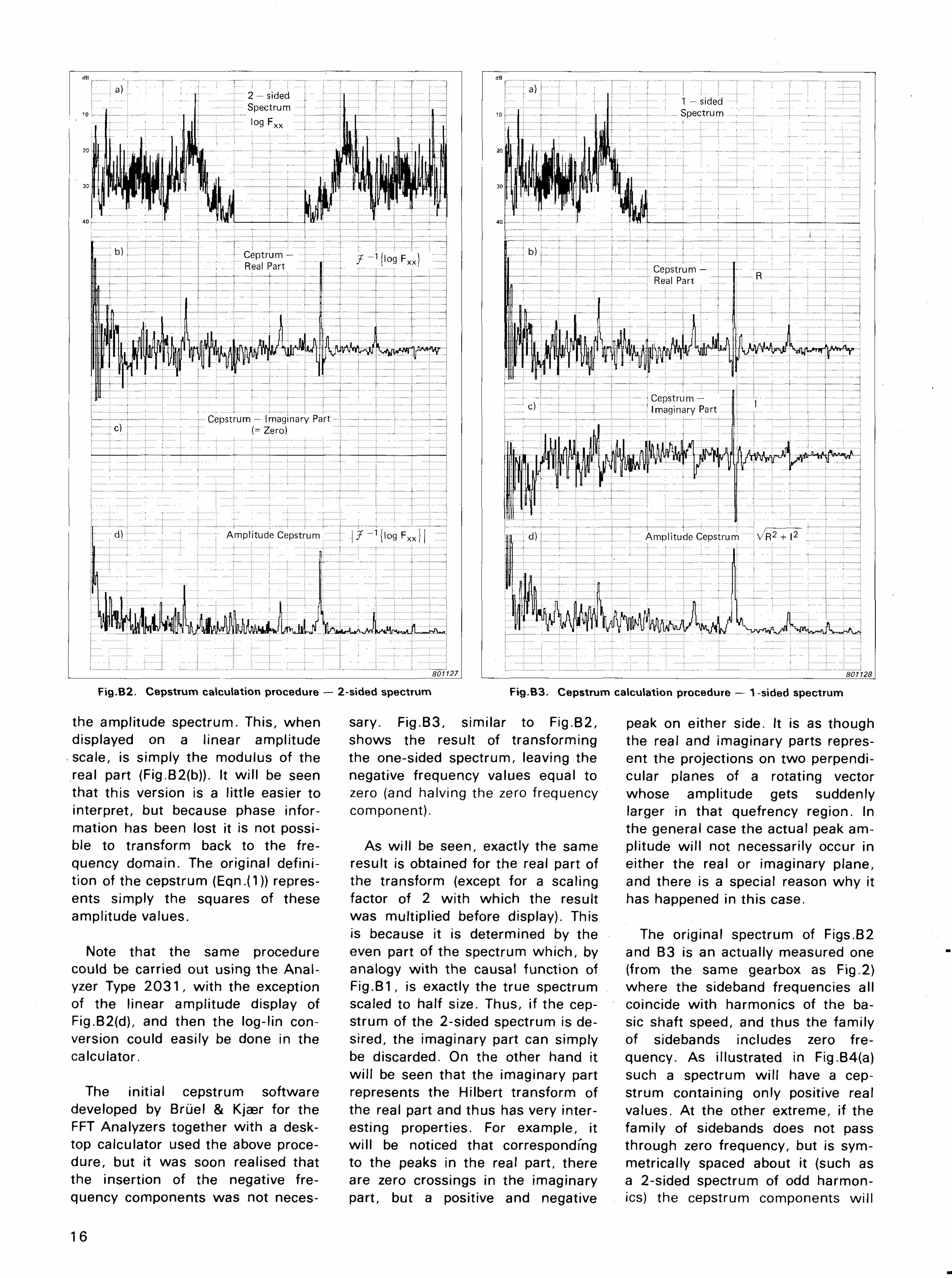
Fig.B2. Cepstrum calculation procedure — 2-sided spectrum Fig.B3. Cepstrum calculation procedure — 1-sided spectrum

the amplitude spectrum. This, when sary. Fig.B3, similar to Fig.B2, peak on either side. It is as though displayed on a linear amplitude shows the result of transforming the real and imaginary parts repres-scale, is simply the modulus of the the one-sided spectrum, leaving the ent the projections on two perpendi-real part (Fig.B2(b)). It wil l be seen negative frequency values equal to cular planes of a rotating vector that this version is a little easier to zero (and halving the zero frequency whose amplitude gets suddenly interpret, but because phase infor- component). larger in that quefrency region. In mation has been lost it is not possi- the general case the actual peak am­ble to transform back to the fre- As will be seen, exactly the same plitude will not necessarily occur in quency domain. The original defini- result is obtained for the real part of either the real or imaginary plane, tion of the cepstrum (Eqn.(1)) repres- the transform (except for a scaling and there is a special reason why it ents simply the squares of these factor of 2 with which the result has happened in this case. amplitude values. was multiplied before display). This

is because it is determined by the The original spectrum of Figs.B2 Note that the same procedure even part of the spectrum which, by and B3 is an actually measured one

could be carried out using the Anal- analogy with the causal function of (from the same gearbox as Fig.2) yzer Type 2 0 3 1 , with the exception Fig.BI , is exactly the true spectrum where the sideband frequencies all of the linear amplitude display of scaled to half size. Thus, if the cep- coincide with harmonics of the ba-Fig.B2(d), and then the log-lin con- strum of the 2-sided spectrum is de- sic shaft speed, and thus the family version could easily be done in the sired, the imaginary part can simply of sidebands includes zero fre-calculator. be discarded. On the other hand it quency. As illustrated in Fig.B4(a)

wil l be seen that the imaginary part such a spectrum wil l have a cep-The initial cepstrum software represents the Hilbert transform of strum containing only positive real

developed by Bruel & Kjaer for the the real part and thus has very inter- values. At the other extreme, if the FFT Analyzers together with a desk- esting properties. For example, it family of sidebands does not pass top calculator used the above proce- will be noticed that corresponding through zero frequency, but is sym-dure, but it was soon realised that to the peaks in the real part, there metrically spaced about it (such as the insertion of the negative fre- are zero crossings in the imaginary a 2-sided spectrum of odd harmon-quency components was not neces- part, but a positive and negative ics) the cepstrum components will

16

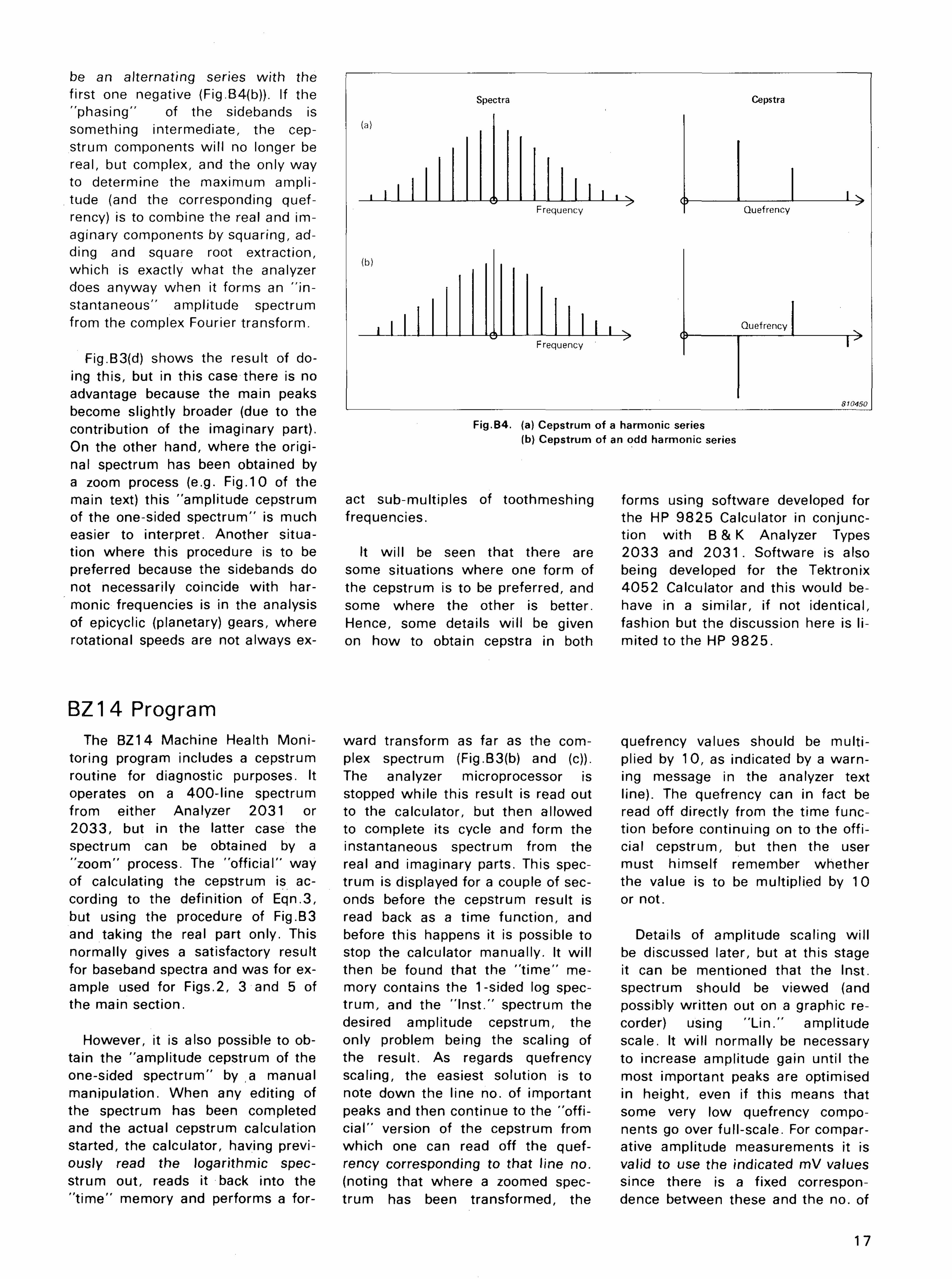
be an alternating series with the first one negative (Fig.B4(b)). If the "phasing" of the sidebands is something intermediate, the cep-strum components will no longer be real, but complex, and the only way to determine the maximum ampli­tude (and the corresponding quef-rency) is to combine the real and im­aginary components by squaring, ad­ding and square root extraction, which is exactly what the analyzer does anyway when it forms an " in ­stantaneous" amplitude spectrum from the complex Fourier transform.

Fig.B3(d) shows the result of do­ing this, but in this case there is no advantage because the main peaks become slightly broader (due to the contribution of the imaginary part). On the other hand, where the origi­nal spectrum has been obtained by a zoom process (e.g. Fig.10 of the main text) this "amplitude cepstrum of the one-sided spectrum" is much easier to interpret. Another situa­tion where this procedure is to be preferred because the sidebands do not necessarily coincide with har-monic frequencies is in the analysis of epicyclic (planetary) gears, where rotational speeds are not always ex-

BZ14 Program The BZ14 Machine Health Moni­

toring program includes a cepstrum routine for diagnostic purposes. It operates on a 400-line spectrum from either Analyzer 2031 or 2033, but in the latter case the spectrum can be obtained by a "zoom" process. The "official" way of calculating the cepstrum is ac­cording to the definition of Eqn.3, but using the procedure of Fig.B3 and taking the real part only. This normally gives a satisfactory result for baseband spectra and was for ex­ample used for Figs.2, 3 and 5 of the main section.

However, it is also possible to ob­tain the "amplitude cepstrum of the one-sided spectrum" by a manual manipulation. When any editing of the spectrum has been completed and the actual cepstrum calculation started, the calculator, having previ­ously read the logarithmic spec-strum out, reads it back into the " t ime" memory and performs a for-

Fig.B4. (a) Cepstrum of a harmonic series (b) Cepstrum of an odd harmonic series

act sub-multiples of toothmeshing forms using software developed for frequencies. the HP 9825 Calculator in conjunc­

tion with B & K Analyzer Types It wil l be seen that there are 2033 and 2 0 3 1 . Software is also

some situations where one form of being developed for the Tektronix the cepstrum is to be preferred, and 4052 Calculator and this would be-some where the other is better. have in a similar, if not identical, Hence, some details will be given fashion but the discussion here is li­on how to obtain cepstra in both mited to the HP 9825.

ward transform as far as the com- quefrency values should be multi­plex spectrum (Fig.B3(b) and (c)). plied by 10, as indicated by a warn-The analyzer microprocessor is ing message in the analyzer text stopped while this result is read out line). The quefrency can in fact be to the calculator, but then allowed read off directly from the time func-to complete its cycle and form the tion before continuing on to the offi-instantaneous spectrum from the cial cepstrum, but then the user real and imaginary parts. This spec- must himself remember whether trum is displayed for a couple of sec- the value is to be multiplied by 10 onds before the cepstrum result is or not. read back as a time function, and before this happens it is possible to Details of amplitude scaling will stop the calculator manually. It wil l be discussed later, but at this stage then be found that the " t ime" me- it can be mentioned that the Inst. mory contains the 1-sided log spec- spectrum should be viewed (and trum, and the "Inst." spectrum the possibly written out on a graphic re-desired amplitude cepstrum, the corder) using "L in . " amplitude only problem being the scaling of scale. It wil l normally be necessary the result. As regards quefrency to increase amplitude gain until the scaling, the easiest solution is to most important peaks are optimised note down the line no. of important in height, even if this means that peaks and then continue to the "offi- some very low quefrency compo-cial" version of the cepstrum from nents go over full-scale. For compar-which one can read off the quef- ative amplitude measurements it is rency corresponding to that line no. valid to use the indicated mV values (noting that where a zoomed spec- since there is a fixed correspon-trum has been transformed, the dence between these and the no. of

17

0 : " 4 0 0 0 LINE CEPSTRUM": 1 : d im A$ [ 8 0 0 0 + 1 + 16] 2 : b u f " I N " , A $ , 3 3 : 20-C 4 : e n t "CENTRE LINE OF FIRST SPECTRUM?",C 5 : i f C<20 o r O 3 8 0 ; d s p "WRONG ANSWER";wait 5 0 0 ; j m p - 1 6: 10-N 7: e n t "NUMBER OF SPECTRA?",N 8 : i f ( N - l ) * 4 0 + O 3 8 0 ; d s p "WRONG ANSWER";wai t 5 0 0 ; j m p - 1 9 : N M 0 0 + L 1 0 : w t b 7 2 5 , " # l , K 0 , L 0 , R l , O 0 ; " 1 1 : f o r 1=1 t o N 1 2 : fxd 0 ; w t b 7 2 5 , " # 1 , H , " , s t r ( 4 0 ( 1 - 1 ) + C - 1 ) , " ; " 1 3 : w a i t 2000 1 4 : w t b 7 2 5 , " # 5 ; " 1 5 : t f r 7 2 5 , " I N " , 8 0 0 1 6 : jmp r d s ( " I N " ) # - l 1 7 : cmd 7 , " _ " 1 8 : n e x t I 1 9 : d s p "SCALING OF SPECTRUM" 2 0 : o-s 2 1 : f o r 1=1 t o L 2 2 : S + i t f ( A $ [ 2 I - 1 , 2 I ] ) - S 2 3 : n e x t I 2 4 : S /L+S 2 5 : f o r 1=1 t o L 2 6 : f t i ( ( i t f ( A $ [ 2 1 - 1 , 2 1 ] ) - S ) * 3 2 ) + A $ [ 2 1 - 1 , 2 1 ] 2 7 : n e x t I 2 8 : 1-C 2 9 : w t b 7 2 5 , , , # 1 , K 0 , L 2 , I 0 ; " 3 0 : 1025+C 3 1 : w t b 7 2 5 , " # 9 , " 3.2: f o r 1=1 t o N 3 3 : fxd 0 ; w t b 7 2 5 , " # 1 , E , " , s t r ( 4 0 0 ( 1 - 1 ) + C + 5 1 1 ) , " ; " 3 4 : w t b 7 2 5 , " # 2 , 1 6 , 1 , " ,A$ [ 8 0 0 ( 1 - 1 ) + 1 , 8 0 0 1 ] ;cmd 7 , " ? " 3 5 : n e x t I 3 6 : fxd 0 ; w t b 7 2 5 , " # 1 , E , " , s t r ( C + 5 1 1 ) , " ; " 3 7 : w t b 7 2 5 , " # 1 , H 1 9 ; H

3 8 : d s p 3 9 : e n d * 1 8 8 7 2

810050

Fig.B5. Program listing for obtaining cepstrum of up to 4000-line spectrum

dB they represent. Thus, to obtain To proceed to the official cep-comparative cepstra it is sufficient strum it is sufficient to press "con-to ensure that the full-scale level in t inue" on the calculator. mV is the same.

Zoom Cepstra With the Analyzer Type 2033 it is

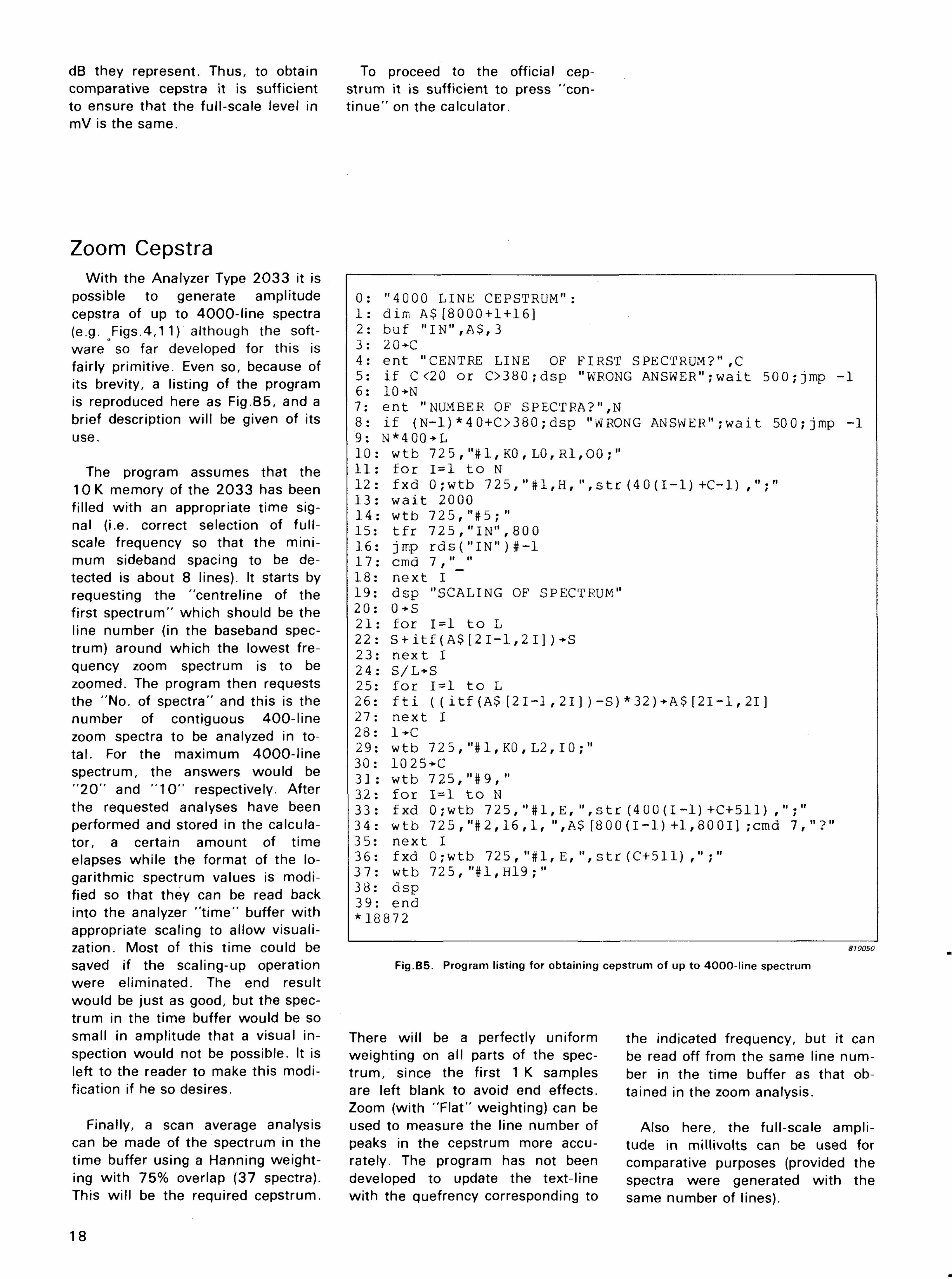
possible to generate amplitude cepstra of up to 4000-l ine spectra (e.g. Figs.4,1 1) although the soft­ware so far developed for this is fairly primitive. Even so, because of its brevity, a listing of the program is reproduced here as Fig.B5, and a brief description wil l be given of its use.

The program assumes that the 10 K memory of the 2033 has been filled with an appropriate time sig­nal (i.e. correct selection of ful l-scale frequency so that the mini­mum sideband spacing to be de­tected is about 8 lines). It starts by requesting the "centreline of the first spectrum" which should be the line number (in the baseband spec­trum) around which the lowest fre­quency zoom spectrum is to be zoomed. The program then requests the "No. of spectra" and this is the number of contiguous 400-line zoom spectra to be analyzed in to­tal. For the maximum 4000-l ine spectrum, the answers would be " 2 0 " and " 1 0 " respectively. After the requested analyses have been performed and stored in the calcula­tor, a certain amount of time elapses while the format of the lo­garithmic spectrum values is modi-

r

fied so that they can be read back into the analyzer " t ime" buffer with appropriate scaling to allow visuali­zation. Most of this time could be saved if the scaling-up operation were eliminated. The end result would be just as good, but the spec­trum in the time buffer would be so small in amplitude that a visual in­spection would not be possible. It is left to the reader to make this modi­fication if he so desires.

Finally, a scan average analysis can be made of the spectrum in the time buffer using a Hanning weight­ing with 75% overlap (37 spectra). This wil l be the required cepstrum.

18

Fig.B5. Program listing for obtaining cepstrum of up to 4000- l ine spectrum

There will be a perfectly uniform the indicated frequency, but it can weighting on all parts of the spec- be read off from the same line num-trum, since the first 1 K samples ber in the time buffer as that ob-are left blank to avoid end effects. tained in the zoom analysis. Zoom (with "Flat" weighting) can be used to measure the line number of Also here, the full-scale ampli-peaks in the cepstrum more accu- tude in millivolts can be used for rately. The program has not been comparative purposes (provided the developed to update the text-line spectra were generated with the with the quefrency corresponding to same number of lines).

Amplitude Calibration For the two types of cepstrum dis­

cussed herein (i.e. the inverse trans­form cepstrum of Eqn.(3), or the am­plitude cepstrum just described) the amplitude scale is linear, but the units are dB. This is because the original input to the cepstrum calcu­lation is a logarithmic spectrum wi th units of dB, and the units of an amplitude spectrum are the same as those of the t ime signal be­ing transformed, e.g. Volts. Thus, provided one knows the correspon-dance between the dB range of the original spectrum, and the number of volts representing this range when the log spectrum is treated as a t ime signal, it is easy to make the conversion. However, in order to make cepstra as comparable as pos­sible, the fol lowing calibration proce­dure is recommended, as it is the one adopted for the BZ14 program. Note that as remarked in the main text, it is still only valid to compare cepstra made wi th the same analy­sis parameters and w i th the same noise level in the spectrum.

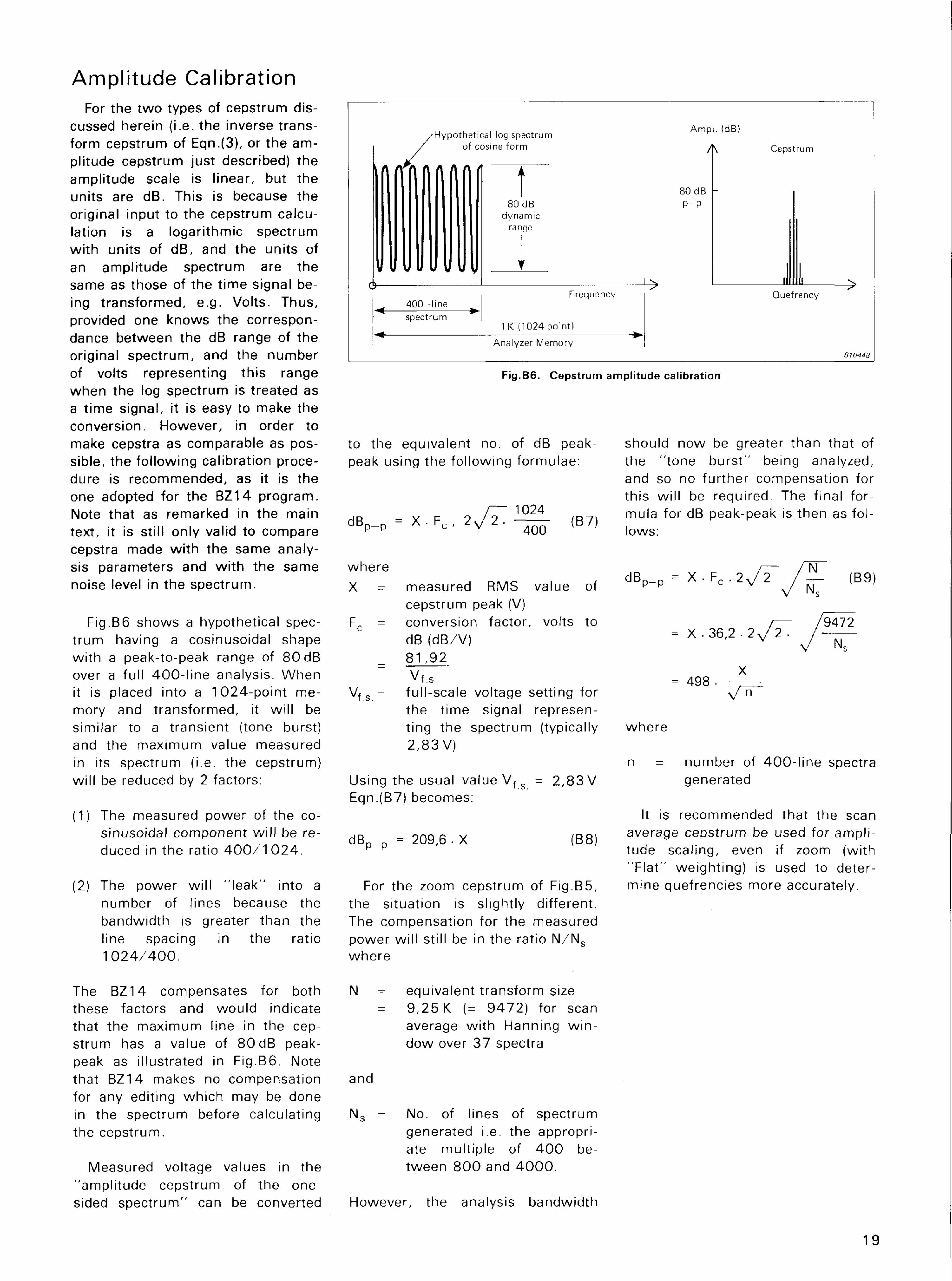
Fig.B6 shows a hypothetical spec­trum having a cosinusoidal shape wi th a peak-to-peak range of 80 dB over a ful l 400- l ine analysis. When it is placed into a 1024-point me­mory and transformed, it wi l l be similar to a transient (tone burst) and the maximum value measured in its spectrum (i.e. the cepstrum) wi l l be reduced by 2 factors:

(1) The measured power of the co-sinusoidal component wi l l be re­duced in the ratio 4 0 0 / 1 0 2 4 .

(2) The power wi l l " leak" into a number of lines because the bandwidth is greater than the line spacing in the ratio 1 0 2 4 / 4 0 0 .

The BZ14 compensates for both these factors and would indicate that the maximum line in the cep­strum has a value of 80 dB peak-peak as illustrated in Fig.B6. Note that BZ14 makes no compensation for any editing which may be done in the spectrum before calculating the cepstrum.

Measured voltage values in the "amplitude cepstrum of the one­sided spectrum" can be converted

19

should now be greater than that of the "tone burst" being analyzed, and so no further compensation for this wi l l be required. The final for­mula for dB peak-peak is then as fol­lows:

dBp_p = X-F c .2y2~ / 5 T (B9) V l̂ s

/ — /9472 = X .36,2 -2J2 ■ /

X = 498 - — =

where

n = number of 400- l ine spectra generated

It is recommended that the scan average cepstrum be used for ampli­tude scaling, even if zoom (with "F la t " weighting) is used to deter­mine quefrencies more accurately.

Fig.B6. Cepstrum amplitude calibration

to the equivalent no. of dB peak-peak using the fol lowing formulae:

/ — 1024 dB p _ p = X . F C . 2 ^ 2 - - ^ <B7)

where X = measured RMS value of

cepstrum peak (V) Fc - conversion factor, volts to

dB (dB/V) 8 1 , 9 2 Vf.s.

Vf s - full-scale voltage setting for the t ime signal represen­ting the spectrum (typically 2 ,83V)

Using the usual value V f s = 2,83 V Eqn.(B7) becomes:

dB p _ p = 209,6- X (B8)

For the zoom cepstrum of Fig.B5, the situation is slightly different. The compensation for the measured power wi l l still be in the ratio N /N s

where

N = equivalent transform size = 9,25 K (= 9472) for scan

average wi th Hanning w in ­dow over 37 spectra

and

N s = No. of lines of spectrum generated i.e. the appropri­ate multiple of 4 0 0 be­tween 8 0 0 and 4 0 0 0 .

However, the analysis bandwidth

References LCh i lde rs , D.G., Skinner, D.P. & 5. Mitchell, L.D., & Lynch, G.A., 1 1. Drosjack, M.J. & Houser, D.R.,

Kemerait, R.C., "The Cepstrum: "Origins of Noise", Machine De- "An Experimental and Theoreti-A Guide to Processing". IEEE sign, May 1, 1 969. cal Study of the Effects of Simu-Proc. Vol. 65, No. 10, October lated Pitch Line Pitting on the 1977, pp. 1428—1443 . 6. Kohler, H.K., Pratt, A. & Thomp- Vibration of a Geared System".

son, A .M . , "Dynamics and ASME Paper No.77-DET-123, 2. Noll, A . M . , "Cepstrum Pitch De- Noise of Parallel-axis Gearing" September 1977.

terminat ion", J.A.S.A. Vol. 4 1 , in "Gearing in 1 9 7 0 " , I. Mech. No.2, 1967, pp. 293—309 . E., London. 12. Papoulis, A., "The Fourier Inte­

gral and its Applications", 3. Bogert, B.P., Healy, M.J.R. & 7. White, C.J., "Detection of Gear- McGraw-Hil l , 1 962.

Tukey, J.W., "The Quefrency Al- box Failure", Workshop in On-anysis of Time Series for Condition Maintenance, ISVR, Echoes: Cepstrum, Pseudo-Au- Southampton Jan. 5—-6, 1972. tocovariance, Cross-cepstrum and Saphe Cracking", in Pro- 8. Thrane, N., "Zoom-FFT", Bruel ceedings of Symposium on & Kjaer Technical Review, Time Series Analysis by Rosen- No.2, 1980. blatt, M., (Ed.), Wiley, N.Y. 1963, pp. 209—243 . 9. Thompson, R.A. and Weich-

brodt, B., "Gear Diagnostics 4. Wirt , L.S., "An ampiitude-modu- and Wear Detection". ASME

lation theory for gear-induced vi- Paper 69 VIBR-1 0, 1 969. brations", Strain Gauge Read­ings, Vol. V, No.4, Oct.—Nov. 10. Randall, R.B., "Frequency Ana-1962. lysis", Bruel & Kjaer publica­

t ion, 1977.

20