1

Bridging and Bonding Social Capital: Which type is good for economic growth?

Paper submitted to ERSA 2003 Jyvaskila (Finland)

Sjoerd Beugelsdijk* and Sjak Smulders** Tilburg University

CentER/Faculty of Economics Warandelaan 2 PO Box 90153

5000 LE Tilburg

* corresponding author; e-mail: s.beugelsdijk@uvt.nl

Abstract In this paper we develop a model of growth and social capital, and test it using data from the European Value Studies (EVS). Following Putnam’s distinction between bonding and bridging social capital, we model social capital as participation in two types of social networks: first, closed networks of family and friends, and, second, open networks that bridge different communities. Agents have a preference for socialising, which they trade off against material well-being. Participation in both social networks is time-consuming and comes at the cost of participation in the formal economic sphere and working time. Through this channel, higher levels of social capital may crowd out economic growth. In addition, participation in intercommunity networks reduces incentives for rent seeking and cheating. Through this channel, higher level of bridging social capital may enhance economic growth. Testing the model, we find that regional differences in materialistic attitudes and the value attached to family life significantly reduce the participation in open networks and that this in turn reduces regional output growth in Europe. Keywords: social capital, economic growth, Europe, EVS JEL codes: O40, R11, Z13 Acknowledgement: The authors want to thank Lans Bovenberg, Patrick Francois, Ton van Schaik, Michael Woolcock, John Helliwell, Jeroen van de Ven, Jacques Hagenaars, Wil Arts, Loek Halman and the other member of the EVS working group for useful comments and suggstions.

2

1. Introduction Most of our time is spent in the presence of others. We spend our working time, leisure time, and family hours with others. However, preferences for socialising differ among individuals and cultures. As Fukuyama puts it, ‘Some [societies] show a markedly greater proclivity for association than others, and the preferred form of association differ. In some, family and kinship constitute the primary form of association; in others, voluntary associations are much stronger and serve to draw people out of their families’ (1995, p. 28). Moreover, socialising is time-consuming and may be traded-off against other activities. Participation in the economy and market exchange (working and shopping) compete with social activities, family life and voluntary organisations.

We may expect that cultural differences affect the degree to which individuals are more oriented to personal possessions and status. These variations in materialistic attitudes result in different levels of socialising. What is especially interesting is how these differences in social structure in turn affect economic outcomes. Are countries or regions in which materialistic attitudes dominate characterized by fast economic growth, or does scarcity of socialising somehow hamper growth? Is socialising with family friends and citizens a good in its own, for which some material benefits are happily given up? Or is socialising also instrumental in promoting material well-being and increasing economic growth?

To study the link between socialising and economic performance, the concept of social capital has been developed, which is often related to trust. Trust and interaction among citizens may stimulate economic growth, when trust facilitates transactions and reduces transaction and monitoring costs in economic exchange. Trust arises mainly within groups with strong social network ties. The repeated interaction among group members prevents opportunistic behaviour and cheating in prisoners’ dilemma kind of situations. Thus, the formation and maintenance of networks constitutes social capital that works as a productive asset in the economy.

However, social interaction and the exploitation of social capital may work in the opposite direction. Closed networks may acts as organisations that lobby and act against the interests of other groups. Rent-seeking behaviour reduces overall well-being as a zero-sum (or even negative-sum) game. Corruption often relies on strong personal connections and extortion practices by mafias may operate through personal connections.

In this paper we aim at formalising and testing the double-sided role of social networks on growth. We model social capital as participation in two types of social networks: first, closed networks of family and friends, and, second, open networks that bridge different communities. Agents have a preference for socialising, which they trade off against material well-being. Participation in both social networks is time-consuming and comes at the cost of participation in the formal economic sphere and working time. Through this channel, higher levels of social capital may crowd out economic growth. In addition, participation in intercommunity networks reduces incentives for rent seeking and cheating. Through this channel, higher level of bridging social capital may enhance economic growth. Testing the model, we find that regions of which the inhabitants are more materialistic and attach more value to family life have significantly lower bridging social capital, which in turn reduces regional output growth in Europe.

The two types of social networks we distinguish correspond to Putnam’s (2000) concepts. He defines ‘bridging social capital’ as bonds of connectedness that are formed across diverse social groups, whereas ‘bonding social capital’ cements only homogenous groups. The added value of this paper lies in the formal macroeconomic modelling and the empirical testing of the influence of different types of social capital on economic growth. We show that bridging social capital has a positive effect on growth, whereas bonding social

3

capital has a negative effect on the degree of sociability outside the closed social circle. We find evidence for Fukuyama’s claim that ‘the strength of the family bond implies a certain weakness in ties between individuals not related to one another’ (Fukuyama, 1995, p. 56). Moreover, we show that an important mechanism that influences the degree to which people are willing to step out of their closed social circle with the associated advantages and build bridging social capital depends on the materialistic attitude of that people. People who are more materialistic tend to stick to the type of socialising that has a direct payoff, whereas less materialistic people are more embedded in social structures that do not directly yield materialistic or worldly advantages.

The rest of the paper is structured as follows. We first review the main ideas in the literature on social capital and materialistic attitudes. Then we present our economic model in which we show the different channels through which the different types of social capital affect economic growth and what the role of materialistic attitude is. Readers not interested in the details of economic theoretic modelling can move directly to Section 4 in which we summarize in a less formal way the testable implications of the model and formulate the central hypothesis to be tested. In section 5 we describe the data. Section 6 presents our empirical estimations for 54 European regions using the European Values Studies (EVS). We conclude with a discussion on our findings and suggest future research questions. 2. Background Social capital is the key theme of our paper. There is not a single unified or generally accepted theory of social capital. The field of social capital ranges across the whole social sciences, from economics, organisational sociology to political science. As Fine states, ‘social capital provides a technological umbrella for grouping together an extraordinarily diverse range of casually constructed illustrations’ (Fine, 2001, p. 78). An important reason for the fuzziness of the concept is caused by the fact that researchers from different disciplines use social capital for what at first sight seem to be entirely different objects of study. When organisation scholars discuss social capital they think of it in terms of the network a firm is embedded in and the resources and limitations this network may provide (e.g. Burt, 1992; Coleman, 1988; Gulati, 1999). When macro-economists and political scientists use social capital, they also think of it in terms of networks, but then referring to networks of associational activity, which is not the same as the previous type of networks (e.g. Putnam, 1993, 2000; Knack and Keefer, 1997). For a better understanding of the theoretical concept of social capital and its cause and effect structure, it is necessary to break down the concept of social capital in two levels, i.e. at the level of the firm (micro) and of the nation state (aggregate level), (cf. Glaeser et. al., 2002). At the individual level, social capital refers to the network an individual belongs to. Individuals derive benefits from knowing others with whom they form networks of interconnected agents. The network enhances access to and exchange of information, enforcement of contracts, and focusing on a shared vision and collective goals. (Nahapiet and Goshal, 1998). At the aggregate level, it is argued that nations or regions can hold different levels of social capital which affects the level of democracy and economic growth (Fukuyama, 1995; Putnam, 1993, 2000; Beugelsdijk and Van Schaik, 2001)). Social capital at this level refers to the social structure that enhances the effectiveness of local governments through traditions of civic engagement and the structure of civic networks.

At both levels the effects of social capital can be positive and negative. At the micro-level, dense networks may provide useful resources such as improved quality of information, a means for control, influence and power, and also a closed social network may encourage

4

compliance with local – sometimes implicit – rules and customs and reduce the need for formal monitoring. However, the danger of closed social networks lies in the fact that the relation specific capital that is developed over time may lead to a tendency to stick to existing linkages and networks start to suffocate (Nooteboom, 2002). This may result in a loss of flexibility and lock-in.

At the aggregate level, the effects of social capital are empirically harder to prove and less clear. Although Putnam (1993) claims to have proven that more social capital in Italian regions is positively correlated with effective governance and economic performance, he has been especially criticised for the method and the lack of a theoretical mechanism between social capital and the other ‘dependent’ variables (Jackman and Miller, 1996; Tarrow, 1996; Dekker et al., 1997; Harris and DeRenzio, 1997; Paxton, 1999; Torsvik, 2000; Boggs, 2001). Boix and Posner attempt to describe mechanisms through which social capital is translated into better economic performance. They argue, among other things, that social capital may reduce the probability of individuals to engage in opportunistic behaviour. This saves on resources devoted to monitoring agent’s performance and makes more resources available for more productive investments.1

In a later work, Putnam (2000) has made a distinction between ‘bridging social capital’ in which bonds of connectedness are formed across diverse social groups, and ‘bonding social capital’ that cements only homogenous groups. Bonding social capital has negative effects for society as a whole, but may have positive effects for the members belonging to this closed social group or network. Bridging social capital, hence, making contacts between different groups or networks is positive. At the micro level this is related to Burt’s theory of structural holes, where the optimal position for an individual is between several groups (Burt, 1992).

The literature on social capital has mainly focused on what constitutes social capital, on the differences in its structure, and the consequences, rather than on explanations where social capital comes from (cf. Glaeser et. al., 2002). Since social capital is formed through network participation and social interaction in groups, it may well arise as a by-product of social interaction that is initiated mainly for other reasons. As argued above, man simply has a desire for socialising, just like it has a preference for food, shelter and material possessions. Our argument is that there may be a trade-off between satisfying materialistic wants and desires for socialising. Materialistic attitudes may thus come at the cost of socialising and reduce the accumulation of social capital.

Materialism, materialistic attitudes and acquisitive desires are studied in the marketing literature and studies on (business) ethics and economic psychology. Belk (1984, 1985) defines materialism as the importance that possessions play in an individual’s life or the importance one attaches to their worldly possessions. Materialism is seen as a personal trait measured along the dimensions of envy, possessiveness and non-generosity. We are more interested in materialism as a value. Richins and Dawson (1992) approach materialism as beliefs on the value of material objects. They measure it along three dimensions: how central is acquisition, how much is it used as the pursuit of happiness, how important is possession-defined success. The study by Inglehart (1997) comes closest to our approach to materialism: he is also interested in the connection between economic development and materialism. In his view, high levels of development correlate with post-materialism, in which material consumption becomes less important relative to the consumption of services

1 Boix and Posner also mention that a) social capital contributes to effective governance by facilitating the articulation of citizen’s demands, b) social capital reduces the need to secure compliance by creating complex and costly mechanisms of enforcement and reduces transaction costs in the arena of citizen-government relations and c) social capital encourages the articulation of collective demands that are to everyone’s benefit.

5

and civic liberties. In our view, the degree of materialism affects economic development through its effect on social capital.

We try to bring together some aspects of social capital at the micro level and the aggregate level and establish links with materialism. In our theoretical model, individuals endogenously choose how much time they spend on closed networks and open networks, depending on their preferences and the opportunity costs. Both networks provide opportunities for social interaction, for which individuals have a preference2. Participation in open networks has the side-effect of protection against opportunistic behaviour by others. Each individual also optimally chooses time spent on rent-seeking activities, on work and on investment and learning. At the aggregate level, participation in open networks (i.e. bridging capital) translates in civic engagement. If the level of civic engagement is high in society, opportunistic behaviour becomes less attractive for individuals and a more efficient system of exchange stimulates the economy. We formally link these mechanisms to investment and economic growth and show that more bridging social capital may (but need not) go together with faster growth. The reason why bridging capital is not necessarily good for growth is that it requires the maintenance of networks, which is a time-consuming process and comes at the cost if working time3.

Our empirical model follows closely the structure of the theoretical model. By doing so, we aim to counter (parts of) the criticism raised by Durlauf (2002, p. F474) on the empirical social capital literature. He writes that empirical studies seem to be particularly plagued by vague definition of concepts, poorly measured data, absence of appropriate exchangeability conditions, and lack of information necessary to make identification claims possible. Moreover, he writes that these problems are especially important as social capital arguments depend on underlying socio-psychological relations that are difficult to quantify, let alone measure. Our paper is a modest attempt to try to counter these criticisms. In our paper, network participation is an endogenous variable so that the effect of social capital, formed through network participation, on growth requires a careful way of testing. In particular, we need to find relevant exogenous factors that determine simultaneously the level of social capital and economic growth. In accordance with the model, we use materialistic attitudes as an instrument: a preference for materialistic aspects of life relative to the social aspects of life directly affects network participation, and it affects growth only indirectly through network participation. The European Value Study provides the data on materialistic attitudes and social capital. Our results show that materialism can indeed explain the level of bridging social capital and that bridging social capital is positively correlated with economic growth. 3. The Model

2 In this respect, Putnam mentions the (Yiddish) distinction between machers and schmoozers (Putnam, 2000, 93-115). People who invest a lot of time in formal organizations are called machers, while those who spend many hours in informal conversation are termed schmoozers. 3 It is important to note that for atomistic agents any form of social interaction – be it either bridging or bonding social capital – yields benefits. The issue is that bridging social capital has a larger (positive) impact on economic growth than bonding social capital. Hence, we do not claim that socialising with family and close friends is a bad activity as such. The crucial point is the distinction between types of socialising; investing in bridging social capital is better from a growth perspective. In this respect Putnam (2000) makes a relevant distinction between ‘getting by’ (bonding social capital) and ‘getting ahead’ (bridging social capital).

6

3.1. Individuals’ static decision problem Individuals care about produced consumption goods (c) and social interaction4 (s). That is, their utility function has both material goods and social aspects as arguments: ( , )u U c s= , , 0c sU U > , where subscripts to function symbols denote (partial) derivatives.

Social interaction is defined as participating in social networks, so that higher levels of network participation can be labelled as higher levels of social capital. We distinguish two types of networks. First, social interaction takes place with close friends and family (which we categorize as f-networks). Second, networks consist of more remote contacts outside the family, within and outside the community one lives, in clubs, pubs and public meeting places, in voluntary organisations (called v-networks). In Putnam’s (2000) terms, f-networks and v-networks represent bonding and bridging capital, respectively. Interacting with others is possible in both of these networks, so that they are substitutes to a certain degree in satisfying the individual’s preference for social interaction. As Fukuyama argues ‘People are embedded in a variety of social groups – families, neighbourhoods, networks, businesses churches, and nations – against whose interests they have to balance their own’ (Fukuyama, 1995, p. 21). However, each network type has its own specific type of social interaction: among friends and family feelings of affection and safety can be nurtured; among more remote contacts other interests may be pursued like self-realisation, social status seeking, information exchange, adventurous contacts with less known ideas and cultures. Hence, on balance the two are substitutes but imperfect ones in the utility function, which is reflected in the sub-utility function for satisfaction from social interaction (s): ( , )s S f v= , , 0f vS S > .

Here, f (v) is the intensity of participation in f-networks (v-networks), to be measured by the time devoted to it. A convenient specification of the (sub)utility function is a constant elasticity of substitution (CES) function, in which two important parameters play a role: one indicating the relative weight of the arguments, and the other indicating how easily the two can be substituted for each other. The specifications are:

( ) /( 1)1/ ( 1) / ( 1) /( , )cs cs

cs cs cs cs csU c s c sσ σ −σ σ − σ σ − σ= µ + ,

( ) /( 1)1/ ( 1) / ( 1) /( , )cf cf

vf vf vf vf vfS f v f vσ σ −σ σ − σ σ − σ= φ + .

The relative importance of material consumption is denoted by µ and will be referred to as the materialism preference parameter. The importance of f-networks relative to v-networks is denoted by φ and will be referred to as the family ties preference parameter. The elasticities

of substitution between the two types of social networks is denoted by vfσ , that between

material consumption and social interaction by csσ . Individuals choose how much they consume and how much they engage in social

interaction. Their choices are constrained by a crucial time (or budget) constraint.

4 From now on, when we write social interaction we mean socialising or sociability. In general, social interaction can also imply the fighting of a war, whereas socialising implies informal friendly social interaction. Nevertheless, in the remainder we restrict social interaction to the process of socialising.

7

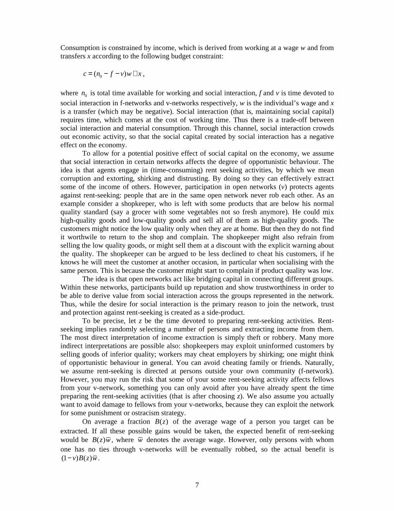
Consumption is constrained by income, which is derived from working at a wage w and from transfers x according to the following budget constraint: 0( )c n f v w x= − − + , where 0n is total time available for working and social interaction, f and v is time devoted to social interaction in f-networks and v-networks respectively, w is the individual’s wage and x is a transfer (which may be negative). Social interaction (that is, maintaining social capital) requires time, which comes at the cost of working time. Thus there is a trade-off between social interaction and material consumption. Through this channel, social interaction crowds out economic activity, so that the social capital created by social interaction has a negative effect on the economy.

To allow for a potential positive effect of social capital on the economy, we assume that social interaction in certain networks affects the degree of opportunistic behaviour. The idea is that agents engage in (time-consuming) rent seeking activities, by which we mean corruption and extorting, shirking and distrusting. By doing so they can effectively extract some of the income of others. However, participation in open networks (v) protects agents against rent-seeking: people that are in the same open network never rob each other. As an example consider a shopkeeper, who is left with some products that are below his normal quality standard (say a grocer with some vegetables not so fresh anymore). He could mix high-quality goods and low-quality goods and sell all of them as high-quality goods. The customers might notice the low quality only when they are at home. But then they do not find it worthwile to return to the shop and complain. The shopkeeper might also refrain from selling the low quality goods, or might sell them at a discount with the explicit warning about the quality. The shopkeeper can be argued to be less declined to cheat his customers, if he knows he will meet the customer at another occasion, in particular when socialising with the same person. This is because the customer might start to complain if product quality was low.

The idea is that open networks act like bridging capital in connecting different groups. Within these networks, participants build up reputation and show trustworthiness in order to be able to derive value from social interaction across the groups represented in the network. Thus, while the desire for social interaction is the primary reason to join the network, trust and protection against rent-seeking is created as a side-product.

To be precise, let z be the time devoted to preparing rent-seeking activities. Rent-seeking implies randomly selecting a number of persons and extracting income from them. The most direct interpretation of income extraction is simply theft or robbery. Many more indirect interpretations are possible also: shopkeepers may exploit uninformed customers by selling goods of inferior quality; workers may cheat employers by shirking; one might think of opportunistic behaviour in general. You can avoid cheating family or friends. Naturally, we assume rent-seeking is directed at persons outside your own community (f-network). However, you may run the risk that some of your some rent-seeking activity affects fellows from your v-network, something you can only avoid after you have already spent the time preparing the rent-seeking activities (that is after choosing z). We also assume you actually want to avoid damage to fellows from your v-networks, because they can exploit the network for some punishment or ostracism strategy.

On average a fraction ( )B z of the average wage of a person you target can be extracted. If all these possible gains would be taken, the expected benefit of rent-seeking would be ( )B z w , where w denotes the average wage. However, only persons with whom one has no ties through v-networks will be eventually robbed, so the actual benefit is (1 ) ( )v B z w− .

8

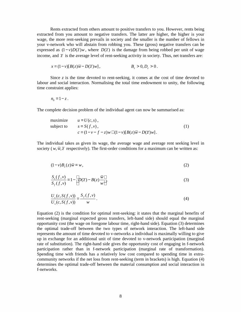
Rents extracted from others amount to positive transfers to you. However, rents being extracted from you amount to negative transfers. The latter are higher, the higher is your wage, the more rent-seeking prevails in society and the smaller is the number of fellows in your v-network who will abstain from robbing you. These (gross) negative transfers can be expressed as (1 ) ( )v D z w− , where ( )D z is the damage from being robbed per unit of wage income, and z is the average level of rent-seeking activity in society. Thus, net transfers are: (1 )[ ( ) ( ) ]x v B z w D z w= − − , 0, 0z zB D> > .

Since z is the time devoted to rent-seeking, it comes at the cost of time devoted to labour and social interaction. Normalising the total time endowment to unity, the following time constraint applies: 0 1n z= − . The complete decision problem of the individual agent can now be summarised as: maximize ( , )u U c s= , subject to ( , )s S f v= , (1)

(1 ) (1 )[ ( ) ( ) ]c v f z w v B z w D z w= − − − + − − . The individual takes as given its wage, the average wage and average rent seeking level in society ( , ,w w z respectively). The first-order conditions for a maximum can be written as: (1 ) ( )zv B z w w− = , (2)

( , )

1 ( ) ( )( , )

v

f

S f v wD z B z

S f v w = − −

, (3)

( , )( , ( , ))

( , ( , ))fc

s

S f vU c S f v

U c S f v w= . (4)

Equation (2) is the condition for optimal rent-seeking: it states that the marginal benefits of rent-seeking (marginal expected gross transfers, left-hand side) should equal the marginal opportunity cost (the wage on foregone labour time, right-hand side). Equation (3) determines the optimal trade-off between the two types of network interaction. The left-hand side represents the amount of time devoted to v-networks a individual is maximally willing to give up in exchange for an additional unit of time devoted to v-network participation (marginal rate of substitution). The right-hand side gives the opportunity cost of engaging in f-network participation rather than in f-network participation (marginal rate of transformation). Spending time with friends has a relatively low cost compared to spending time in extra-community networks if the net loss from rent-seeking (term in brackets) is high. Equation (4) determines the optimal trade-off between the material consumption and social interaction in f-networks.

9

3.2. Static equilibrium under symmetry The decisions of the individual agent depend on the society-wide variables like average rent-seeking, which in turn depend on the decisions of others. To solve for the macro-economic levels of the variables, we employ the simple assumption of complete symmetry: all agents have the same preferences and income and will make the same choices. Hence we have ,z z w w= = . (5) We can now also link the benefits of rent-seeking to the losses. We assume that if all agents engage in the same intensity of rent-seeking, the losses are a constant factor 1+ ζ larger than the benefits: ( ) (1 ) ( )D z B z= + ζ , 0ζ > . (6) Thus rent-seeking is a negative sum game: what the extorter gains, is less than the damage to the person being extorted. Part of the transfer may be lost “in the battle” or confiscated by authorities. One might also see this as an implicit way of modelling the costs that the victim has to incur to avoid cheating and shirking (monitoring costs). Parameter ζ captures this externality cost of rent-seeking.5

Our main question in this subsection is how economic activity (c) and bridging social capital (v) are related. Note that both variables are endogenous. Therefore, we need to identify how variations in exogenous variables simultaneously affect economic performance and social capital. The exogenous driving forces in the model are labour productivity (w), preference for family and friends ties ( φ ), and preference for material consumption (materialism µ ). We reduce the model to two equations in terms of the endogenous variables c and v and the exogenous variables , ,w φ µ . First note from (2) and (5), that z is a negative function of v:

( )z Z v= , 0vZ < . (7) Next, substitute this result and (6) into (3) to find that f is a positive function of v and

φ:

( ; )f F v= φ , , 0vF Fφ > . (8)

Substituting these results into the budget constraint, we find:

[1 ( ; ) ( ) (1 ) ( ( ))]c w v F v Z v v B Z v= − − φ − − − ζ

( ; , )T v w≡ φ , 0, 0wT Tφ < > . (9)

This is a key result. It reveals that networks have an impact on the economy through

five channels (corresponding to the five places where v shows up in the equation). First, more social interaction in v-networks directly reduces labour time and hence reduces output (see second term in brackets). Second, different types of social networking are positively correlated, so an increase in v-networking also increases time spent with friends and family

5 We think that it is realistic to add this negative externality. However, all our qualitative results go through when ζ=0.

10

and further reduces working time (third term in brackets). Together, we call these effects the labour time crowding out effect. The other three effects stem from the fact that v-capital protects against rent-seeking. In more dense social networks, rent-seeking is less, so that not only time is freed up for production (fourth term in brackets, recall that Z depends negatively on v), but also the negative sum externality is smaller (through lower probability that non-members meet and rob each other and through the smaller rent-seeking effort z). Whether economic activity is positively or negatively related with v-networks depends on whether the negative labour time crowding out effect dominates or not the positive protection against rent-seeking effect.

Equation (9) also reveals that materialism (µ ) has no direct impact on the economy, but can have an indirect impact only through affecting v. Indeed, from (4), we find (after substituting the solutions for f and z) another equation in c and v, which depends on all key exogenous variables, including µ:

( ; , , )c C v w= φ µ , , , 0v wC C Cµ > . (10)

In the appendix we derive a more precise solution by linearizing the model. We can prove that C increases in v, µ and w, but that the impact of φ cannot be unambiguously signed. This relationship shows that consumption and v-networks are positively related. The reason is simply that social interaction and material consumption goods are normal goods: richer persons spend more on both. As expected, more materialistic preferences (higher µ) or higher income (w) result in higher consumption for given v. A stronger preference for family ties (higher φ) has two opposite effects: it shifts attention away from material consumption (substitution effect), but it also implies that a given level of interaction with family and friends generates more utility from social interaction (cf. income effect). The latter effect makes material consumption scarcer relative to social interaction (s) and tends to raise c.

The two equations (9) and (10) simultaneously solve for the two endogenous variables, material consumption (c) and bridging capital (v). The two equations can be represented as the lines labeled T and C, respectively, in a simple diagram in the v,c plane (we draw lines instead of curves to stress that results are based on comparative statics, see appendix). The slope of the T-line is ambiguous because of the opposing labour time effect and protection effect. The upper and lower panels of Figure 1 represent the two possibilities.

We illustrate the working of our model by showing the effects of an increase in the materialism preference parameter (µ), which is a key determinant in our analysis. More materialistic attitudes make the C-line shift to the left. The point of equilibrium moves along the T-line. In the upper panel, the slope of T is negative since the labour time crowding out effect dominates; then consumption rises and bridging social capital falls. In the lower panel, T slopes upward since the protection effect dominates; then both consumption and social capital fall. Hence, materialism affects the economy (as measured by a change in c) through a change in voluntary organizations (a movement along the T-curve), but whether it boosts or hurt the economy depends on the relative strength of the crowding-out effect and protection-against-rent-seeking effect.

<Insert Figure 1 about here>

11

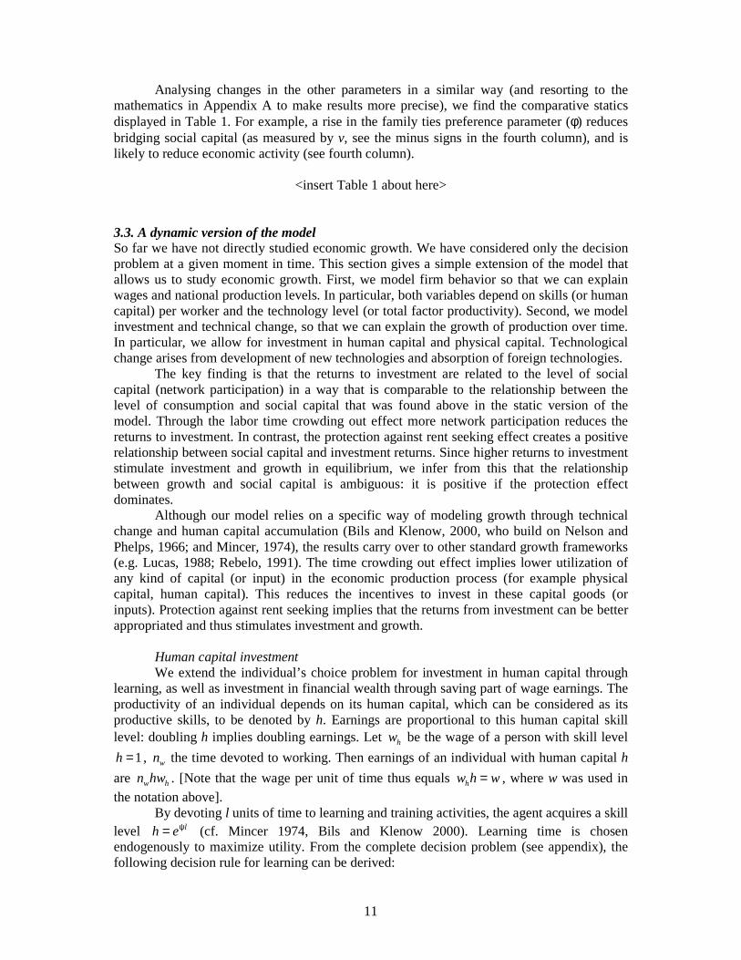
Analysing changes in the other parameters in a similar way (and resorting to the mathematics in Appendix A to make results more precise), we find the comparative statics displayed in Table 1. For example, a rise in the family ties preference parameter (φ) reduces bridging social capital (as measured by v, see the minus signs in the fourth column), and is likely to reduce economic activity (see fourth column).

<insert Table 1 about here> 3.3. A dynamic version of the model So far we have not directly studied economic growth. We have considered only the decision problem at a given moment in time. This section gives a simple extension of the model that allows us to study economic growth. First, we model firm behavior so that we can explain wages and national production levels. In particular, both variables depend on skills (or human capital) per worker and the technology level (or total factor productivity). Second, we model investment and technical change, so that we can explain the growth of production over time. In particular, we allow for investment in human capital and physical capital. Technological change arises from development of new technologies and absorption of foreign technologies. The key finding is that the returns to investment are related to the level of social capital (network participation) in a way that is comparable to the relationship between the level of consumption and social capital that was found above in the static version of the model. Through the labor time crowding out effect more network participation reduces the returns to investment. In contrast, the protection against rent seeking effect creates a positive relationship between social capital and investment returns. Since higher returns to investment stimulate investment and growth in equilibrium, we infer from this that the relationship between growth and social capital is ambiguous: it is positive if the protection effect dominates.

Although our model relies on a specific way of modeling growth through technical change and human capital accumulation (Bils and Klenow, 2000, who build on Nelson and Phelps, 1966; and Mincer, 1974), the results carry over to other standard growth frameworks (e.g. Lucas, 1988; Rebelo, 1991). The time crowding out effect implies lower utilization of any kind of capital (or input) in the economic production process (for example physical capital, human capital). This reduces the incentives to invest in these capital goods (or inputs). Protection against rent seeking implies that the returns from investment can be better appropriated and thus stimulates investment and growth.

Human capital investment We extend the individual’s choice problem for investment in human capital through

learning, as well as investment in financial wealth through saving part of wage earnings. The productivity of an individual depends on its human capital, which can be considered as its productive skills, to be denoted by h. Earnings are proportional to this human capital skill level: doubling h implies doubling earnings. Let hw be the wage of a person with skill level

1h = , wn the time devoted to working. Then earnings of an individual with human capital h

are w hn hw . [Note that the wage per unit of time thus equals hw h w= , where w was used in the notation above].

By devoting l units of time to learning and training activities, the agent acquires a skill level lh eψ= (cf. Mincer 1974, Bils and Klenow 2000). Learning time is chosen endogenously to maximize utility. From the complete decision problem (see appendix), the following decision rule for learning can be derived:

12

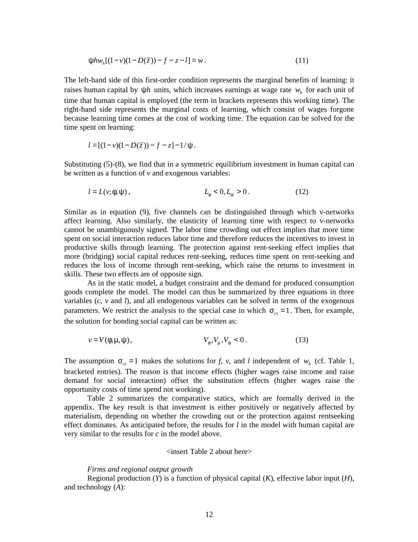
[(1 )(1 ( )) ]hhw v D z f z l wψ − − − − − = . (11)

The left-hand side of this first-order condition represents the marginal benefits of learning: it raises human capital by hψ units, which increases earnings at wage rate hw for each unit of time that human capital is employed (the term in brackets represents this working time). The right-hand side represents the marginal costs of learning, which consist of wages forgone because learning time comes at the cost of working time. The equation can be solved for the time spent on learning: [(1 )(1 ( )) ] 1/l v D z f z= − − − − − ψ . Substituting (5)-(8), we find that in a symmetric equilibrium investment in human capital can be written as a function of v and exogenous variables:

( ; , )l L v= φ ψ , 0, 0L Lφ ψ< > . (12)

Similar as in equation (9), five channels can be distinguished through which v-networks affect learning. Also similarly, the elasticity of learning time with respect to v-networks cannot be unambiguously signed. The labor time crowding out effect implies that more time spent on social interaction reduces labor time and therefore reduces the incentives to invest in productive skills through learning. The protection against rent-seeking effect implies that more (bridging) social capital reduces rent-seeking, reduces time spent on rent-seeking and reduces the loss of income through rent-seeking, which raise the returns to investment in skills. These two effects are of opposite sign. As in the static model, a budget constraint and the demand for produced consumption goods complete the model. The model can thus be summarized by three equations in three variables (c, v and l), and all endogenous variables can be solved in terms of the exogenous parameters. We restrict the analysis to the special case in which 1csσ = . Then, for example, the solution for bonding social capital can be written as: ( , , )v V= φ µ ψ , , , 0V V Vφ µ ψ < . (13)

The assumption 1csσ = makes the solutions for f, v, and l independent of hw (cf. Table 1, bracketed entries). The reason is that income effects (higher wages raise income and raise demand for social interaction) offset the substitution effects (higher wages raise the opportunity costs of time spend not working).

Table 2 summarizes the comparative statics, which are formally derived in the appendix. The key result is that investment is either positively or negatively affected by materialism, depending on whether the crowding out or the protection against rentseeking effect dominates. As anticipated before, the results for l in the model with human capital are very similar to the results for c in the model above.

<insert Table 2 about here>

Firms and regional output growth Regional production (Y) is a function of physical capital (K), effective labor input (H),

and technology (A):

13

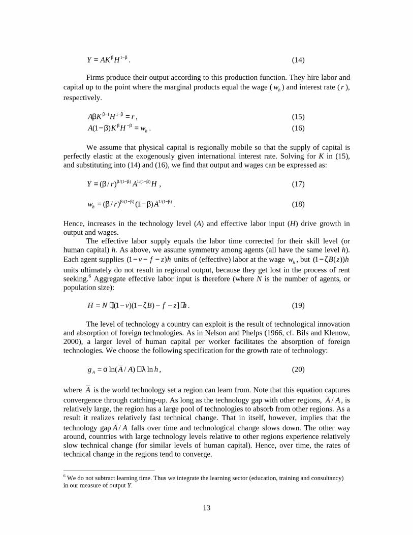
1Y AK Hβ −β= . (14)

Firms produce their output according to this production function. They hire labor and

capital up to the point where the marginal products equal the wage ( hw ) and interest rate ( r ), respectively.

1 1A K H rβ− −ββ = , (15)

(1 ) hA K H wβ −β−β = . (16) We assume that physical capital is regionally mobile so that the supply of capital is

perfectly elastic at the exogenously given international interest rate. Solving for K in (15), and substituting into (14) and (16), we find that output and wages can be expressed as: /(1 ) 1/(1 )( / )Y r A Hβ −β −β= β , (17) /(1 ) 1/(1 )( / ) (1 )hw r Aβ −β −β= β − β . (18) Hence, increases in the technology level (A) and effective labor input (H) drive growth in output and wages.

The effective labor supply equals the labor time corrected for their skill level (or human capital) h. As above, we assume symmetry among agents (all have the same level h). Each agent supplies (1 )v f z h− − − units of (effective) labor at the wage hw , but (1 ( ))B z h− ζ units ultimately do not result in regional output, because they get lost in the process of rent seeking.6 Aggregate effective labor input is therefore (where N is the number of agents, or population size): [(1 )(1 ) ]H N v B f z h= ⋅ − − ζ − − ⋅ . (19)

The level of technology a country can exploit is the result of technological innovation and absorption of foreign technologies. As in Nelson and Phelps (1966, cf. Bils and Klenow, 2000), a larger level of human capital per worker facilitates the absorption of foreign technologies. We choose the following specification for the growth rate of technology: ln( / ) lnAg A A h= α + λ , (20) where A is the world technology set a region can learn from. Note that this equation captures convergence through catching-up. As long as the technology gap with other regions, /A A , is relatively large, the region has a large pool of technologies to absorb from other regions. As a result it realizes relatively fast technical change. That in itself, however, implies that the technology gap /A A falls over time and technological change slows down. The other way around, countries with large technology levels relative to other regions experience relatively slow technical change (for similar levels of human capital). Hence, over time, the rates of technical change in the regions tend to converge.

6 We do not subtract learning time. Thus we integrate the learning sector (education, training and consultancy) in our measure of output Y.

14

Growth of per capita output can now be calculated as:

ln( / ) ln ln(1 )1yg Y H y v f z l

λ= α − α + α − − − + α + ψ − β

[(1 )(1 ) ] /

[(1 )(1 ) ]

dl d v B f z dt

dt v B f z

− − ζ − −+ψ +− − ζ − −

, (21)

where per capita output is denoted by /y Y N≡ , where we have used (17) to eliminate /A A

and /Y H is the average income per unit of human capital in rest of the world. In our model we can ignore the last two terms if (due to the assumption 1csσ = ) l, v, f, and z are constant over time. In terms of testing the model, these terms are expected to be relatively small. Moreover, no time series data is available for these variables.

We are then left with three relevant terms that explain growth: the foreign income level, own income level, and the term in brackets, which can be written in terms of v and the parameters φ and ψ only (see (12), (8), (7), (6)).

• The first term at the right-hand side of (21) captures spillover effect: rich neighboring regions provide a region with the opportunities to learn from and grow faster.

• The second term at the right-hand side of (21) captures beta-convergence. Poor countries grow faster than rich countries, ceteris paribus, due to the technological catch-up effect just described.

• The third term at the right-hand side of (21) captures the effect of social capital on growth. Note that the sign is ambiguous because the labor time allocation effect may or may not be dominated by the protection against rent-seeking effect. Also the effect of ψ is ambiguous: on the one hand a higher productivity of learning enhances human capital, on the other hand it reduces hours worked.

Of course, v is an endogenous variable, but its solution is already given in (13): materialistic attitudes, investment opportunities and family ties preferences affect the level of bridging social capital. Interesting to note is that materialism may be good or bad for growth. In particular, if the protection against rent-seeking effect dominates, more materialism leads to lower bridging capital and thus to lower growth. 4. The hypothesis In the theoretical model, the following results have been derived about the relationship between growth and social interaction.

• Growth and bridging social capital are endogenous variables, which are simultaneously determined by attitudes towards spending time with friends and family, materialism, and the productivity of investment.

• Controlling for family ties, initial income, and productivity of investment, an exogenous increase in bridging capital may affect growth negatively or positively. In the former case, the time cost of networking dominates the productive benefits. The latter case arises if the protection of bridging capital against rent-seeking is strong enough (see equations (21) and (12)).

• Materialism affects growth only through bridging social capital. • Family ties, investment and materialism negatively affect bridging capital. Initial

income does not affect bridging capital (see (13)).

15

Figure 2 summarizes the model predictions. Arrows with plus (minus) sign denote positive (negative) relationships between two variables. In the next section we explain the background of the data and test the above hypotheses.

<insert figure 2 about here> 5. Measurement

In order to test the above hypotheses we investigate 54 European regions. By taking regions, we are able to test if Putnam’s thesis on social capital based on Italian regions can be generalized (Putnam, 1993). Moreover, a European regional approach allows us to incorporate Temple’s critical comment (1999) that countries differing widely in social, political and institutional characteristics are unlikely to fall on a common surface. Most important, however, is the fact that by comparing national cultures, ‘we risk losing track of the enormous diversity found within many of the major nations of the world’ (Smith and Bond 1998, 41). By studying regions and regional differences this risk is limited.

Data on social capital are taken from the European Value Studies (EVS), which is a survey on norms and values. The European Values Study is a large-scale, cross-national, and longitudinal survey research program on basic human values, initiated by the European Value Systems Study Group (EVSSG) in the late 1970s. The EVS aimed at designing and conducting a major empirical study of the moral and social values underlying European social and political institutions and governing conduct. Its coordination centre is located at Tilburg University, The Netherlands7. Our data refer to 1990. The set comprises 7 countries, i.e. France, Italy, Germany, Spain, The Netherlands, Belgium, and the United Kingdom. In order to compare the data on norms and values with regional economic data we used the Eurostat definition of regions. The regional level in our analyses is the NUTS1 level. This implies that France consists of 8 regions, Italy 11, Germany 11 (former eastern regions excluded), Spain 7, The Netherlands 4, Belgium 3, and the UK 10 (including Scotland, excluding Northern Ireland). The total number of regions equals 54.Table 3 and figure 4 provide an overview of the regions included in our analysis.

<insert figure 4 and table 3 about here> Our theoretical model and its implications summarized above closely guide our empirical model. We can distinguish two main features of the empirical model, the modeling of growth and the modeling of social attitudes and interaction. In this section we first discuss how we measure economic growth and then how we measure social variables. Economic growth

We follow Barro and Sala-i-Martin (1995) who explain regional growth differentials in Europe between 1950 and 1990. As we have more recent economic data, we analyze the period 1950-19988. To test the growth part of our theoretical model, we use the standard growth framework, in which economic growth is explained by a number of key economic variables (Baumol, 1986; Barro, 1991; Mankiw et. al., 1992; Barro and Sala-i-Martin, 1995).

7 Details regarding the sample size, response rate, the survey questions and the procedures followed to obtain non-culturally biased estimates (e.g. backward translation procedures), are extensively discussed at the website http://evs.kub.nl. We use the 1990 wave as the 1981 and 1999 are not available on the regional level. 8 We also observed shorter periods of analyses for our dependent variable, e.g. the period 1970-1998.

16

Similar to Barro and Sala-I-Martin (1995), we have computed the regional growth figures by relating the regional GDP per capita information to the country mean.9 There are at least two reasons to use the country mean as a correction factor. First of all we do not have regional price data. Second, the figures on regional GDP are provided in an index form that is not comparable across countries. In addition one could argue that by measuring regional growth this way we directly control for national growth rates that may bias the regional growth rates. Hence, we have used Gross Regional Product (GRP) figures that are expressed as deviations from the means from the respective countries. The 1950 data are based on Molle, Van Holst and Smits (1980), whereas the data for Spain refer to 1955 and are based on Barro and Sala-i-Martin’s (1995) calculations. Just as the other economic data, the 1998 data on GRP are drawn from Eurostat information.

Following standard empirical growth models as developed by Barro (1991) we include initial per capita income of the region (INITIAL INCOME), measured relative to the income of the other regions in the country (cf. Barro and Sala-i-Martin 1995). In addition we include a measure to control for the level of welfare of neighboring regions, as is common in regional growth analyses. Low initial income and large spillovers from other regions may stimulate growth by the convergence measure. Ideally one should use interregional input-output tables to calculate regional multipliers and construct a variable that controls for spatial correlation10. However, this information was not available. In order to control for spatial correlation, we applied Quah’s (1996) approach and calculated the so-called neighbor relative income. This method implies that we use average per capita income of the surrounding, physically contiguous regions to control for spatial auto-correlation.. Hence, spillovers (SPILLOVERS) are measured as the average income of the regions adjacent to the region.

Next to initial income, ‘Barro’ regressions typically include measures for human and physical capital. Our proxies for the productivity of investment are educational attainment, national investment rates, and in addition we use a measure for the concentration of human capital in agglomerations (created by the interaction of a dummy variable indicating the major agglomerations in a country and the school enrolment ratio).11. Regions in which large agglomerations are present may benefit from scale economics, concentration of human capital, the presence of a cluster of specialized suppliers, and a market with a critical mass of consumers (network externalities). Further, the idea is that years of schooling (SCHOOLING) facilitate learning on the job (which was theoretically modeled by variables l and h). Schooling is measured by the total number of pupils at first and second level in 1977, divided by total number of people in the corresponding age group. The basic growth period we analyze is 1950-1998. The school enrolment rate in 1977 falls in between these dates and given the fact that school enrolment rates have increased since 1950, the 1977 information is a reasonable proxy for the average over the entire period. Data come from Eurostat. Data on school enrolment rates in Spanish regions refer to 1985.

Since regional investment rates are not available, we take the national rates (INVESTMENT). Apart from availability of reliable regional investment data12, another

9 Gross Regional Product of a region in 1950 is divided by the mean of the Gross Regional Products of all regions belonging to a certain country. A similar formula is applied to calculate the 1998 relative regional product. Regional growth over the period 1950-1998 is then based on these two indices. 10 There exist other ways to have a more refined control variable that can be taken into consideration, for example the physical length of abutting boundaries or the physical characteristics of the border terrain. However, these kinds of extensions go beyond the scope of the current paper. 11 We selected the Western part of the Netherlands, Greater Paris, Greater Berlin, Greater London, Barcelona area, Brussels, and the Italian region Lazio (Rome) as major agglomerations. 12 Eurostat and Cambridge Econometrics do provide data on Gross Fixed Capital Formation. However, data are incomplete for some countries or in time.

17

reason to take the country level investment data, is the underlying assumption of a closed economy. Because of spatial interaction, regional investment figures would only provide a limited understanding of regional economic growth (Nijkamp and Poot 1998). Therefore we have taken the country level data. Data are taken from the Penn World Tables 5.6. The period for which we have calculated the average of the investment ratio is 1950-199213. Bridging social capital To operationalise bridging social capital we follow Knack and Keefer (1997) by exploiting data on membership of certain voluntary associations. We measure bridging social capital by the density of associational activity, or in other words the average per capita membership of an association. Of the associations mentioned in EVS we have used membership of the following groups:

a. Religious or church organizations b. Education, arts, music, cultural activities c. Youth work (e.g. scouts, guides, youth clubs) d. Sports or recreation e. Women’s groups

The groups mentioned under a, b and c were also used by Knack and Keefer (1997) in their analysis of the Putnam groups and the relation with economic growth. We have chosen to add d and e as they also proxy associational activity that is not focused on rent seeking activities that can be expected from groups such as political parties and professional associations14. We expect the selected groups to involve social interaction that builds trust and cooperative habits, which is the reason why we label it bridging social capital. The average score of the density of group membership in 54 European regions equals .34 with a standard deviation of .18. The highest score (.80) is obtained in the eastern part of the Netherlands (Oost-Nederland), and the lowest score (.08) in the North-Eastern part of Spain (Noroeste). All data are based on 1990 information. Bonding social capital and family ties We measure preferences for family ties (preference parameter φ in the model) by EVS data on the relative importance of the closed social circle.15 On a scale of 1-4 (very important – not at all important) respondents are asked to indicate the importance in their life of family, and friends and acquaintances. By using factor analysis we re-scaled the two items in one dimension reflecting bonding social capital. Both on the individual and the regional level the chosen items converge into one dimension. The average value of bonding social capital in European regions is -.077. The regions where people attach the highest value to the close social circle can be found in the southern part of Europe. The region with the highest score on bonding social capital is the French Mediterranean (.23) and the region where people attach least importance to family and friends is the German region Bremen (-.46).

13 Penn World Tables 5.6 provides data up to 1992. 14 Olson (1982) observed that associational activity may hurt growth because of rent-seeking activities. According to Olson, many of these associations may act as special interest groups lobbying for preferential policies that impose disproportionate costs on society. In this respect, Knack and Keefer (1997) distinguish between Putnam and Olson groups. 15 We have no measures of time spent in closed networks (bonding social capital). This means that we cannot test equation (8) of the model. In other words, we look at purely stated preference instead of revealed preference with respect to bonding social capital. Instead, for bridging capital we use a measure closer to a revealed preference indicator (actual network participation).

18

Materialism To operationalise the degree of materialistic attitude towards society we use two proxies. First we use the well-known materialism-postmaterialism that Inglehart (1997, 2000) introduced. It is based on the relative importance respondents attach to the following items:

a. Maintaining order in the nation b. Giving people more say in important government decisions c. Fighting rising prices d. Protecting freedom of speech

Of each of these four statements respondents are asked to indicate the most important and the next most important statement. The materialist/postmaterialist value is created as follows. If the respondent’s first and second choices are both materialist items (i.e. maintaining order and fighting rising prices), the score is ‘1’. If the respondent’s first and second choices are both postmaterialist items (i.e. giving people more say and protecting free speech), the score is ‘3’. If the two choices are any mixture of materialist and postmaterialist items, the score is ‘2’. In sum, a high score on this variable reflects a postmaterialistic attitude and a low score reflects a materialistic attitude. The mean score equals 2.04 with a maximum value of 2.29 in the region Berlin (Germany). The most materialistic according to Inglehart’s materialism index are the people in the Italian region Campania (1.68).

In addition to the operationalisation of materialism based on Inglehart, we used a second proxy. EVS contains several questions on the importance people attach to various aspects of a job. Based on the question ‘which of the following aspects of a job you personally think are important?’ respondents are asked to indicate a number of aspects.16 Among these aspects some refer to materialistic values (e.g. good pay) and others to immaterialistic values (e.g. useful job for society). We selected the following items that reflect an immaterialistic attitude towards a job:

a. pleasant people to work with; b. a useful job for society; and c. meeting people.

Using factor analysis we re-scaled these items into one dimension and aggregated the individual scores to mean scores for each of our 54 regions. The variable is scaled from immaterialistic to materialistic. We choose to label this variable job-related materialism. Hence, high scores on the variable job related materialism reflect a materialistic attitude. The highest score (most materialistic) is obtained in the French region Sud-Ouest (.56). The lowest score can be found in the eastern part of the Netherlands (-.58). Table 4 presents descriptive statistics of the variables defined above and used in the empirical tests

<insert table 4 about here> 6. Testing the model Figure 3 depicts our testing strategy. The boxes correspond to the theoretical model in Fgure 2, but the labels now refer to our data. For example, our measure of growth is regional economic growth 1950-1998 and one of our measures for materialism is Inglehart’s index for materialism/postmaterialism.

16 The total list of aspects respondents are asked to choose from is: good pay, pleasant people to work with, not too much pressure, good job security, good chances for promotion, a job respected by people in general, good hours, an opportunity to use initiative, a useful job for society, generous holidays, meeting people, a job in which you feel you can achieve something, a responsible job, a job that is interesting, a job that meets one’s abilities.

19

<insert Figure 3 about here>

Our aim is to test the model in figure 3. In particular, we are interested in the sign of the relationship between growth and bridging capital. Here we have to take into account that bridging social capital and growth are simultaneously determined. To avoid a simultaneity bias, we need to instrument for bridging social capital. Hence we use a two-stage least squares (2SLS) testing strategy.17 In the first stage, we instrument social capital, by regressing our measure of bridging capital on our measures of materialism, family ties and investment productivity. Doing so, we test for the signs of the arrows in the North-East part of the figure (and of equation (13)). In the second stage, we use instrumented bridging capital, together with investment and convergence measures, as regressors for growth. Doing so we test for the signs of the left-hand side of the figure (and of equation (21) with (12) substituted). Needless to say, we are most interested in finding the empirically relevant sign of the relation between growth and bridging social capital which could not be determined a priori and was accordingly denoted by a question mark in figure 2.

The results are summarized in table 5. We estimate different models. The first is our basic model in which our dependent variable is the average regional-economic growth of per capita income between 1950 and 1998. In addition to the basic model we estimate a number of other model specifications.

<insert Table 5 about here>

The basic model in column (1) shows that bridging social capital has a positive and

significant effect on regional growth. Bonding social capital has the negative sign predicted by our model, but is insignificant in the second stage. However, in the first stage, bonding social capital (or better, the preference for family ties) negatively affects bridging capital, in accordance with the model. Also materialism determines bridging capital with the correct sign and significant coefficient. The results on the effects of bridging capital on growth are worth being highlighted. Note that from the model we could not sign this effect unambiguously because of two opposing forces. Empirically, we find a positive effect, which means that bridging capital is good for growth. This positive effect is statistically significant, but quite small in economic terms. A one percent standard deviation in bridging capital raises growth by only 0.17Â���� �����SHUFHQWDJH�SRLQWV��$�DVVHVVPHQW�RI�WKH�HFRQRPLF�VLJQLILFDQFH�of the result that is more consistent with our estimation procedure yields a bigger number: a one standard deviation change in our three instruments (family ties and two types of materialism) raises growth through bridging capital by 0.11 percentage points. Over our 48 years sample period this amounts to the non-negligible increase of 5.4% in (last year’s) regional income.

The social capital variables in the basic model perform even better than the traditional variables like schooling and investment, of which the coefficient is insignificant. While schooling is often a problematic variable in growth regressions (Krueger and Lindahl, 2001), investment usually is a robust variable (Levine and Renelt, 1991). Note however, that we included national rather than regional investment rates.

In model (2) we change our period of observation 1950-1998 into 1984-1998. In this case results of course only change in the second stage, as the dependent variable changes. For our study, the most important change occurs with respect to the direct effect of bonding social 17 We have checked for a possible endogeneity bias by using a Hausman test. It is common to test whether it is necessary to use an instrumental variable and estimate a 2SLS regression, i.e., whether a set of estimates obtained by least squares is consistent or not. We performed an augmented regression and concluded that estimating an OLS would not yield consistent estimates.

20

capital on growth. In model (2) this effect is significantly negative in accordance with the model. This is an improvement relative to our basic model (1), which does not yield a significant direct relationship between growth and bonding social capital. Also remarkable is that the effect of bridging social capital becomes more than twice as large as in the basic model.

At the same time initial income becomes insignificant and schooling and investment become significant. The economic interpretation is that in the more recent period, the process of catching-up is completed and regional (and national) differences play a larger role in explaining growth differentials. The overall fit of this model is worse given the R-squared of .53 in model (1) and .44 in model (2). This is mainly caused by the poor fit of the standard economic variables, especially initial income. Whereas in the longer period of 1950-1998 convergence effects can be observed, our results indicate that for a shorter period 1984-1998 this effect cannot be empirically confirmed. This result is not remarkable and fits the general thought. Other authors have shown that on the European regional level especially in the 80s there was no convergence, some even suggest relative divergence (e.g. Fagerberg and Verspagen, 1995; Maurseth, 2001). In the third, fourth and fifth model specifications we reduced the number of instruments or added one.

Model (3) shows the results when the variable Job related materialism is left out. Compared with the basic model this does not yield different results. Leaving out Inglehart’s materialism index does however yield differences. As model (4) shows, bridging social capital is not significantly positive related to growth as it is in all the other models. The overall fit of the 1st stage model goes considerably down from .58 in model (1) to .43, suggesting it is important to include Inglehart’s materialism index in the 1st stage.

Adding trust as an instrument to the 1st stage regression does not yield differences with the basic model. As analyzed and discussed by Beugelsdijk and Van Schaik (2001), trust is not significantly related to regional economic growth in Europe. The results in table 2 suggest that trust is not indirectly related to growth either. The relation between trust and bridging social capital is not significant when we use trust as an instrument for bridging social capital. In case we add trust as an instrument and exclude the other instruments the above conclusion does not change.

In our last model we tested if the reduction of observations influences our results. We have left out the regions that had the highest and lowest residual in the 2nd stage of our basic regression model (1). The regions left are Schleswig-Holstein (Germany) and Nord Ovest (Italy). The analysis for the reduced sample of 52 regions does not differ greatly of the results obtained in the basic regression on 54 regions. The main difference can be found in the fact that bridging social capital is not related to growth at the 5% significance level, but at 10% (though the reduction in significance is marginal, namely 6% versus 4%).18 7. Conclusion and discussion We have developed a model to formalize the link between social capital, defined as participation in social networks, and economic growth. We identified two channels through which social capital and economic growth can be interrelated. First, network participation is a time-consuming process, which crowds out working and learning time and therefore tends to

18 We also excluded the observations with maximum and minimum value of growth (Bayern in Germany, resp. Nord Ovest in Northern Italy) and the maximum and minimum value for initial income (Hamburg, resp. South Italy). Thirdly, we used a so-called recursive method to check of the composition of the sample influenced our results. All these checks suggest that our results are robust with respect to the potential influence of outliers.

21

be negatively correlated with growth. Second, participation in networks that span different communities may create bridging capital. Trust is generated in these networks, which protects members against rent-seeking activities. The reason is that participants that know each other from the same network restrain their opportunistic behaviour towards each other, to maintain reputation within the group and to avoid ostracism or lighter forms of punishment. By this second channel, the relationship between growth and social capital tends to be positive. Such a positive relationship does not exist for bonding social capital and economic growth. Bonding social capital arises from networking within own communities of close friends and family. Within the own closed circle opportunistic behaviour is checked anyway, so an increase in time spent with your own close circle does not reduce opportunistic behaviour in the economy. Higher levels of bonding social capital are therefore likely to go together with lower rates of economic growth, since spending more time with family and close friends comes at the cost of working and learning time. Our empirical analysis of growth in 54 European regions confirms the importance of the distinction between these two kinds of social capital. Bridging social capital is empirically good for growth, while a large importance attached to family ties is negatively related to growth.

We have also stressed the fact that social capital is a choice variable that has to be explained from deeper economic and cultural variables. We think of cultural values as relatively stable over time and differing markedly across regions (cf. Baker et. al., 1981, Inglehart, 1977, 1997, Rokeach, 1973). The stability of ‘cultural’ variables over time answers the question if it is allowed to explain regional growth differentials in Europe between 1950-1998 and 1984-1998. Moreover, using a shorter period of analysis, e.g. 1991-1998 implies the use of short run growth rates, which are likely to be biased. One of the main contributions of the paper is to provide empirical evidence for the link between differences in culture and social attitudes, on the one hand, and economic performance, on the other hand. A central variable in our analysis is materialism. For our European regional data, more importance attached to material possession is correlated with lower participation in voluntary organizations, which results through reduced bridging social capital in lower growth. Apart from generating explicit results on social values and economic performance, our two-stage approach also allowed us to address the simultaneity problems of which other studies have been criticized (Durlauf, 2002).

In future research, more explicit attention could be paid to the distinction between bridging and bonding social capital. Note that bonding social capital was latent in our analysis. When data are available on actual time spend with family and friends, a more explicit analysis is possible. In this paper, we simplified reality and modeled a choice that individuals face between spending time with their friends in their closed social circle (bonding social capital) and social interaction in external networks (bridging social capital). However, in reality bonding and bridging are not ‘either-or’ categories into which social networks can be neatly divided, but ‘more-or-less’ dimensions along which we can compare different forms of social capital (Putnam, 2000, 23). Many groups or individuals simultaneously bond along some social dimensions and bridge across others. In addition, it can be questioned if materialism is the true driver of the choice between bonding and bridging social capital. The relative amount of bridging versus bonding may not depend on the degree of materialism, but may be a reflection of underlying deeper cultural values, of which materialism is an important component (Inglehart and Baker, 2000).

Future empirical research is also needed to make the connection between the model and the empirics more precise with respect to one of the central mechanisms in our model. Measures of rent-seeking and corruption should be negatively correlated with measures of bridging social capital if our protection against rent-seeking effect is truly relevant.

22

Unfortunately, this type of data on the regional level in Europe is hard to find. Also the theoretical modeling can be refined. In particular, in future work we plan to integrate into our growth framework the microeconomics of reputation, opportunistic behaviour and efficiency losses from cheating. We are convinced that general equilibrium modeling with micro-economic foundation can further our insights in the link between social values and economic performance and can fruitfully guide the empirics of social capital and cultural values.

Literature

Baker, K., R, Dalton, and K. Hildebrandt, 1981, Germany transformed, Cambridge, MA,

Cambridge University Press.

Barro, R.J., and X. Sala-i-Martin 1995. Economic growth. New York: McGraw Hill.

Begg, I. 1995. Factor mobility and regional disparities in the European Union. Oxford Review

of Economic Policy 11.2, 96-112.

Belk, R.W. 1984. Three Scales to Measures Constructs Related to Materialism: Reliability,

Validity and Relationships to Measure Hapiness. In: T. Kinnear (ed) Advances in Consumer

Research vol. 11 (Association for Consumer Research, Provo, UT), 291-297.

Belk, R.W. 1985. Materialism: Trait aspects of living in the material world. Journal of

Consumer Research 12, 265-280.

Beugelsdijk, S. and A.B.T.M. van Schaik, 2001, Social capital and regional economic growth

, CentER Discussion paper 102, Tilburg University.

23

Bils, M. and P.J. Klenow 2000. Does Schooling Cause Growth? American Economic Review

90(5), 1160-1183.

Boggs, Carl 2001. Social capital and political fantasy: Robert Putnam’s Bowling alone.

Theory and Society 30, 281-297

Boix, Charles and Posner, Daniel N. 1998. Social capital: explaining its origins and effects on

government performance. British Journal of Political Science 28, 686-693.

Burt, R. 1992. The social structure of competition. In Networks and organizations, structure,

form and action, ed. Nohria, N., and R. Eccles. Boston M.A: Harvard Business School Press.

Coleman, J.S. 1990. Foundations of social theory. Cambridge: Harvard University Press.

Dekker, Paul, Ruud Koopmans, and Andries van den Broek. 1997. Voluntary associations,

social movements and individual political behaviour in Western Europe: a micro-macro

puzzle. In: Jan W. van Deth (ed.) Private Groups and Public Life: Social participation,

voluntary associations and political involvement in representative democracies. London:

Routledge.

Durlauf, S. 2002. On the empirics of social capital. The Economic Journal 112, p. F459-

F479.

24

Fafchamps, M. and B. Minten 2002. Returns to social network capital among traders. Oxford

Economic Papers 54, 173-206.

Fagerberg, J., and B. Verspagen 1995. Heading for divergence? Regional growth in Europe

reconsidered. MERIT working paper 2/95-014.

Fine, Ben 2001. Social Capital versus Social Theory: Political economy and social science at

the turn of the millennium. New York: Routledge

Francois, P. 2002. Social capital and economic development. London: Routledge.

Fukuyama, F. 1995 Trust: the social virtues and the creation of prosperity. New York: The

Free Press.

Glaeser, E.L., Laibson, D., and B. Sacerdote, 2002, An economic approach to social capital,

The Economic Journal 112, F437-F458.

Gulati, Ranjay 1999. Network location and learning: the influence of network resources and

firm capabilities on alliance formation. Strategic Management Journal 20, 397-420

Harriss, John and Paolo De Renzio 1997. ‘Missing link’ or analytically missing?: the concept

of social capital. Journal of International Development 9, 919-937

Inglehart, R., 1977. The silent revolution: changing values and political styles in advanced

industrial society, Princeton, NJ, Princeton University Press.

25

Inglehart, R. 1997. Modernization and postmodernization: cultural, economic and political

change in 43 societies. Princeton, New Jersey, Princeton University Press.

Inglehart, R and W. Baker. 2000. Modernization, cultural change and the persistence of

traditional values, American sociological review 65, 19-51.

Jackman, Robert W. and Ross A. Miller 1996. A renaissance of political culture? American

Journal of Political Science 40.3, 632-659.

Knack, S., and P. Keefer 1997. Does social capital have an economic pay-off? A cross

country investigation. Quarterly Journal of Economics. 112.4:1251-1288.

Krueger, A.B., and M. Lindahl 2001. Education for growth: why and for whom? Journal of

Economic Literature 39, 1101-1136.

Levine, R., and D. Renelt 1992. A sensitivity analysis of cross-country regressions. American

Economic Review 82(4), 942-963.

Lucas, R.E. 1988. On the Mechanics of Economic Development. Journal of Monetary

Economics 22(1), 3-42.

Maurseth, P.B. 2001. Convergence, Geography and technology. Structural Change and

Economic Dynamics 12, 247-276.

26

Mincer, J. 1974. Schooling, Experience and Earnings. New York: Columbia University

Press.

Molle, W., B. Van Holst and H. Smit 1980. Regional disparity and economic development in

the European Community. Westmead, England: Saxon House.

Nahapiet, Janine, and Sumantra Ghoshal 1998. Social capital, intellectual capital and the

organisational advantage. Academy of Management Review 23, 242-266.

Nelson, R.R. and E.S. Phelps 1966. Investment in humans, technological diffusion and

economic growth. American Economic Review May 1966 (papers and proceedings) 56 (2),

69-75.

Nijkamp, P. and Poot, J. 1998. Spatial perspectives on new theories of economic growth. The

Annals of Regional Science 32, 7-38.

Nooteboom, B., 2002. Trust, forms, foundations, functions, failures and figures. Cheltenham,

UK: Edward Elgar

Olson, M. 1982. The rise and decline of nations. New Haven: Yale University Press.

Paxton, P. 1999. Is social capital declining in the United States? A multiple indicator

assessment. American Journal of Sociology 105, 88-127.

27

Putnam, R.; R. Leonardi and R.Y. Nanetti 1993. Making democracy work. Princeton, New

Jersey: Princeton University Press.

Putnam, R. 2000. Bowling alone: the collapse and revival of American community. New

York: Simon and Schuster.

Quah, D. 1996. Regional convergence clusters across Europe. European Economic Review

40:951-958.

Rebelo, S. 1991. Long-run Policy Analysis and Long-run Growth. Journal of Political

Economy 99 (3), 500-521.

Richins, M.L. and S. Dawson. 1992. A Consumer Values Orientation for Materialism and Its

Measurement: Scale Development and Validation. Journal of Consumer Research 19

(December), 303-316.

Rokeach, M. 1973. The nature of human values. New York: Free Press.

Smith P., and Bond, M. 1998. Social psychology across cultures. London: Prentice Hall

Europe.

Tarrow, S. 1996. Making Social Science Work across Space and Time: A Critical Reflection

on Robert Putnam’s Making Democracy Work. The American Political Science Review 90,

389-398.

Temple, J. 1999. The new growth evidence. Journal of Economic Literature 37, 112-156.

28

Torsvik, G. 2000. Social capital and economic development, a plea for the mechanisms.

Rationality and Society 12, 451-476.

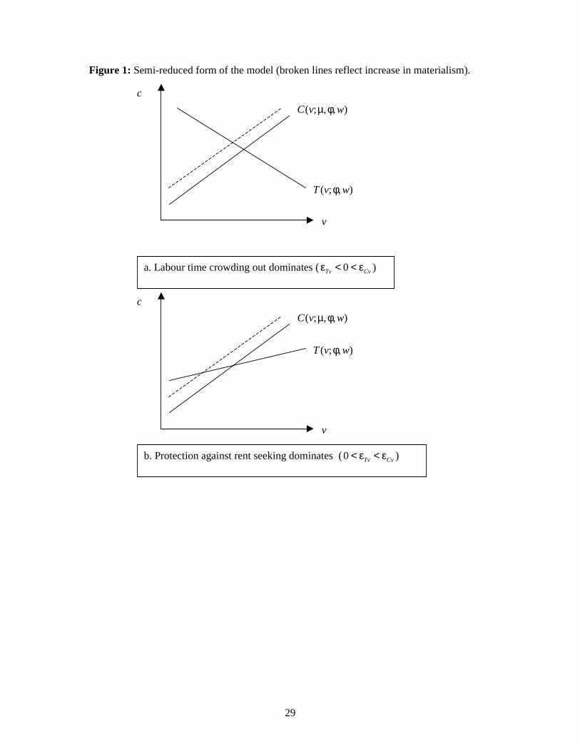
29

Figure 1: Semi-reduced form of the model (broken lines reflect increase in materialism).

v

c

( ; , , )C v wµ φ

( ; , )T v wφ

a. Labour time crowding out dominates ( 0Tv Cvε < < ε )

v

c

( ; , , )C v wµ φ

( ; , )T v wφ

b. Protection against rent seeking dominates ( 0 Tv Cv< ε < ε )

30

Figure 2: graphical representation of the theoretical model ? – + Figure 3: graphical representation of the empirical model (c.f. model 1 in table 2)

Regional-economic growth 1950-1998

Group membership

Importance family and friends

Job-related materialism

Inglehart’s postmaterialism

Standard economic variables: - Initial income - Schooling - Investment - Spillover - Agglomeration

Economic growth ( yg )

Bridging social capital (v)

Family and friends preference parameter (φ )

Materialism preference parameter (µ )

Standard economic variables:

- convergence ( ln / lnY H y− ), - investment (ψ )

Importance family and friends

Family and friends preference parameter (φ ) investment (ψ )

–

–

–

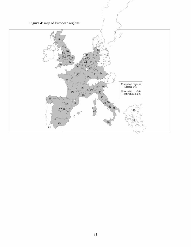
31

Figure 4: map of European regions

3

6

14

10

4443

242

26

19

15

30

37 38

21

1

4 5

7

9

11

12

16

17 18

20

2225

27

28

29

0

0

31 32

33

34

35 36

39

40

4142

45

46

47 48

4950

51

52

53

54

European regionsNUTS1 level

included (54)not included (22)

32

Table 1 Comparative statics, model without investment* Materialism (µ ) Family ties

( φ )*** Labour productivity (w)

1 [ 1]( 1)cs cs csσ < σ = σ >

c v c v c v Labour time crowding out dominates ( 0Tv Cvε < < ε )**

+ – ? – ?[+](+) +[0](–)

Protection against rent seeking dominates ( 0 Tv Cv< ε < ε )

– – – – +[+](?) +[0](–)

* We assume 0Cv Tvε − ε > , which implies that (10) has a steeper slope than (9) in the v,c plane. See appendix A for exact solutions.

** Jiε denotes the elasticity of function J with respect to variable i. See appendix A.

*** The signs in this column are derived for the assumption: , 1vf cs vfσ > σ σ > .

Table 2 Comparative statics, model with human capital* Materialism (µ ) Family ties ( φ ) Investment

productivity ( ψ )

l v l v l v Labor time crowding out dominates ( 0Lvε < )

+ – ? – + –

Protection against rent seeking dominates (0 Lv< ε )

– – – – + –

* We assume 1csσ = , Cv Tvε > ε . See appendix B for exact solutions.

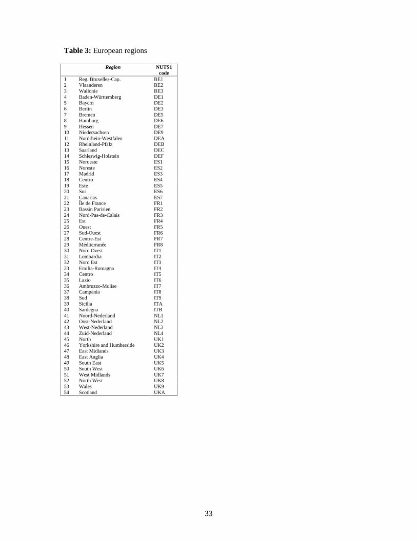
33

Table 3: European regions

Region NUTS1 code

1 Reg. Bruxelles-Cap. BE1 2 Vlaanderen BE2 3 Wallonie BE3 4 Baden-Württemberg DE1 5 Bayern DE2 6 Berlin DE3 7 Bremen DE5 8 Hamburg DE6 9 Hessen DE7 10 Niedersachsen DE9 11 Nordrhein-Westfalen DEA 12 Rheinland-Pfalz DEB 13 Saarland DEC 14 Schleswig-Holstein DEF 15 Noroeste ES1 16 Noreste ES2 17 Madrid ES3 18 Centro ES4 19 Este ES5 20 Sur ES6 21 Canarias ES7 22 Île de France FR1 23 Bassin Parisien FR2 24 Nord-Pas-de-Calais FR3 25 Est FR4 26 Ouest FR5 27 Sud-Ouest FR6 28 Centre-Est FR7 29 Méditerranée FR8 30 Nord Ovest IT1 31 Lombardia IT2 32 Nord Est IT3 33 Emilia-Romagna IT4 34 Centro IT5 35 Lazio IT6 36 Ambruzzo-Molise IT7 37 Campania IT8 38 Sud IT9 39 Sicilia ITA 40 Sardegna ITB 41 Noord-Nederland NL1 42 Oost-Nederland NL2 43 West-Nederland NL3 44 Zuid-Nederland NL4 45 North UK1 46 Yorkshire and Humberside UK2 47 East Midlands UK3 48 East Anglia UK4 49 South East UK5 50 South West UK6 51 West Midlands UK7 52 North West UK8 53 Wales UK9 54 Scotland UKA

34

Table 4: Descriptive Statistics

Mean Std. Dev. Bonding social capital Bridging social capital Materialism-Postmaterialism (Inglehart) Job-related Materialism Investment Schooling Growth 1950-1998 Initial income

-.077 .34

2.04 .059

24.25 .51

.029 -.003

.17

.18

.13

.28 3.74 .067 .33 .25

N=54. Note that ‘Growth 1950-1998’ and ‘Initial income’ are measured relative to the national average for reasons described in the text. The relative high standard deviation for both variables therefore does not have the usual interpretation. Growth is measured in percentage points. Initial income, as well as schooling, investment and bridging social capital are measured in logarithms (see main text for details).

Table 5: IV-regression 2nd Stage Dependent variable: regional economic growth (1) (2) (3) (4) (5) (6) Basic ‘84-‘98 Job-related

Materialism excluded

Inglehart’s Materialism excluded

Trust included as instrument

Regions excluded

Initial income -.92 (.16)** .-.42 (.51) -.92 (.16)** -.92 (.16)** -.92 (.16)** -.84 (.18)** Schooling .49 (.34) 1.71 (.76)** .49 (.35) .50 (.35) .49 (.34) .43 (.35) Investment .33 (.23) 1.28 (.53)** .34 (.23) .33 (.24) .33 (.24) .35 (.24) Spillover .28 (.12)** .64 (.29)** .27 (.12)** .28 (.12)** .28 (.12)** .27 (.13)** Agglomeration .43 (.24)* .30 (.57) .42 (.24)* .44 (.24)* .43 (.24)* .37 (.24) Bonding social capital -.37 (.23) -1.07 (.51)** -.36 (.23) -.39 (.22)* -.37 (.22) -.35 (.23) Bridging social capital .17 (.08)** .46 (.18)** .19 (.08)** .14 (.09) .17 (.08)** .15 (.08)* R-squared .53 .44 .53 .53 .53 .45

N 54 54 54 54 54 52

1St Stage Dependent variable: bridging social capital Bonding social capital -.81 (.37)** -.80 (.36)** -.63 (.38)* -1.02 (.43)** -.82 (.37)** -.81 (.38)** Job-related materialism -.63 (.27)** -.60 (.27)** - -1.35 (.24)** -.57 (.29)** -.63 (.28)** Inglehart’s Postmaterialism 2.53 (.60)** 2.6 (.61)** 3.42 (.49)** - 2.46 (.61)** 2.56 (.62)** Trust - - - - .43 (.63) - R-squared .58 .58 .54 .43 .59 .58

N 54 54 54 54 54 52

Standard errors between parentheses. * indicates 10% significance, ** indicates 5% significance. The basic equation refers to the growth period 1950-1998. We only reported the variables of interest in the first stage and excluded the other exogenous variables. In model 6 we excluded the regions that have the maximum and minimum residual in the second stage of the regression. The regions we excluded are Schleswig-Holstein (Germany) and Nord Ovest (Italy). The regression in model 6 is based on the basic regression as shown in model 1.

35

Mathematical appendix A. Static model Log-linearizing (2), (3), and (4) and the budget constraint in (1), we find after substituting out endogenous variables:

Zvz v+= −ε �� , (7’)

Fvf v= ε + φ� �� , (8’)

( )(1 )Fv Zv Bz Zv

w fwc v f z v v B v w

c c+ + = − − ε + ε + + − ε ε ζ − φ +

�� � � , (9’)

1 [ (1 ) ]1 1

vf csBz Zv Sf vf Sf cs Sf cs

vf

Bc v w

B +

σ − σ ζ= + ε ε ε σ + − ε σ + ε φ + µ + σ − ζ σ − �� � � � .

(10’) Variables with a tilde are logarithmic deviations from the initial equilibrium; variables without a tilde refer to the initial equilibrium; ijε denotes the elasticity of i with respect to j,

and ij+ε denotes the positively defined elasticity of i with respect to j:

/ 0Bz zB z Bε = > ,

/ [0,1]Sf fS f sε = ∈ ,

/ 01

zzZv

z

B zv

v B+−ε = >

−,

1 11Fv vf Bz Zv

B

B +ζε = + σ ε ε >− ζ

.

Note that (7’)-(10’) are the log-linear equivalents of (7)-(10) in the main text; they are used to determine the partial derivatives of the functions Z, F, T and C. B. Dynamic model The complete model reads: maximize [ln ln ] lny oc c sµ + δ + , (B.1)

subject to ( , )s S f v= , (B.2) 1

(1 ) (1 )[ ( ) ( ) ]1

l ly h h oc v f z l e w v B z w D z e w c

rψ ψ= − − − − + − − −

+,

(B.3) where δ is the discount factor and cy and co denote consumption when young and when old, respectively. Note that we assume a Diamond-type of OLG model with logarithmic preferences (which implies 1csσ = ). For simplicity, social interaction matters only for young agents.

The first order conditions can be written as [note that (primed) equation numbers without prefix B correspond to (non-primed) equations in the main text]:

36

(1 ) ( )zv B z w w− = , (2)

( , )

1 ( ) ( )( , )

v

f

S f v wD z B z

S f v w = − −

, (3)

( , )( , ) f

y

S f vS f v

c w

µ = , (4’)

[(1 )(1 ( )) ] 1/l v D z f z= − + − − − ψ , (11’) (1 )o yc r c= δ + . (B.4)

Substituting (11’) and (B.4) in budget constraint (B.3), we find: (1 ) [1/ (1 ) ( ) / ]yc w v B z w w+ δ = ψ + − .

Eliminating yc between this equation and (4’), we find:

( , )

(1 ) [1/ (1 ) ( ) / ]( , )

fS f vv B z w w

S f vµ + δ = ψ + − . (10’)

From now on we focus on symmetry. As before, from (2) we derive ( )z Z v= and from (3) we derive ( ; )f F v= φ . Substituting these results in (11’) and log-linearizing, we find:

[ (1 ) ](1 ) 1Fv Zv Bz Zvv f z v v B fl v

l l l+ +− − ε + ε + + − ε ε + ζ = − φ + ψ ψ

� � �� .

(B.5) Substituting ( )z Z v= and ( ; )f F v= φ into (10’) and log-linearizing, we find:

1 1

(1 )SfV

wv

c

−= ε φ + µ + ψ ε + δ ψ � �� � , (13’)

where

1 (1 ) [ (1 ) ]1 (1 )V Bz Zv Sf vf Sf Bz Zv

B wBv v

B c+ +ζ ε = + ε ε ε σ + − ε + + − ε ε − ζ + δ

>0.

Solving (B.5) and (13’) for l we find:

/ 1Lv Sf Lv Cv Tv

V V V

f ll

l

ε ε + ε ε − ε= − φ − µ + ψ ε ε ε ψ � � �� . (12’)

Equations (13’) and (12’) are used to complete Table 2.