1

Trade Patterns in a Globalised World:

Brazil’s Recent Trajectory Towards

Regressive Specialisation

André Nassif Department of Economics, Fluminense Federal University, Brazil

andrenassif27@gmail.com

Marta dos Reis Castilho Institute of Economics, Federal University of Rio de

Janeiro, Brazil castilho@ie.ufrj.br

Abstract

Globalisation can be defined as the extent and intensity with which a country’s production, trade and capital flows are integrated in the world economy. Our focus is on the globalisation through international trade flows. After analyzing the main theoretical predictions about the effects of global trade integration on trade patterns between countries of different levels of income and technology, this paper investigates the case of Brazil, focusing on its trade integration over the last 26 years (1990-2016). Particularly, we are interested in investigating whether or not (and if so, to what extent) Brazil’s recent trajectory has been directed to a regressive pattern of specialisation. By regressive specialisation we refer to that in which both production and export structures are strongly oriented to goods of low technological sophistication and low income-elasticity of demand. The recent theoretical literature on technological gaps and long-term growth suggests that when a country enters into a quick and sustained regressive pattern of specialisation, its capacity of showing growth rates aligned with its balance-of-payment equilibrium is reduced and, therefore, a falling behind trajectory is observed. Our main empirical findings are (i) the technological gap significantly widened for groups of manufactured goods classified by factor content and technological sophistication; (ii) the income elasticity of demand for Brazilian exports is greater than for Brazilian imports, suggesting a regressive specialisation concentrated in low-tech goods and implying that growth has been constrained by long-term balance-of-payments equilibrium (Thirlwall’s law); and (iii) a very marked trend of high concentration of Brazilian exports in primary goods, but a more diversified basket of imports composed of high technologically sophisticated manufactured goods, reinforcing the regressive specialisation of Brazil’s trade pattern in the last decades.

Keywords: patterns of specialisation; regressive specialisation; diversification; Brazil

JEL classification: F10; F11; F12; F14.

Paper prepared for 21st FMM (Forum for Macroeconomics and Macroeconomic Policies) Conference: “The Crisis of Globalisation” in Berlin, Germany, 9-11 November, 2017, and the 3rd Iberoamerican Socioeconomic Meeting of SASE (Society for the Advancement of Socioeconomics) in Cartagenas de Indias, Colombia, 16-18 November, 2017.

2

1. Introduction

Globalisation can be defined as the extent and intensity with which a country

is integrated in the world economy. Although such integration can and does reach

production, trade and capital flows, our focus is on the globalisation through

international trade flows. Although other earlier waves of economic

internationalisation have happened—from the Industrial Revolution till the beginning

of World War I—, the speed and intensity with which the present wave of trade

globalisation has spread over the entire world economy since the early 1980s has

no precedent in the modern occidental economic history. In fact, from the 1980s

onwards, the rise and diffusion of the microelectronic revolution as well as the

significant reduction of trade barriers also put pressure on most developing countries

to accelerate trade integration into the world economy.

In the case of Brazil, for instance, between 1990 and 1994, after several

decades of protectionist policies adopted under the import substitution development

strategy, the Brazilian government decide to adopt a unilateral and ambitious trade

liberalisation programme, which eliminated most non-trade barriers and reduced

average nominal tariffs for all goods from 30.5% to 11.2%.1 Since several studies

were released in the 1990s and 2000s with the goal of evaluating the impacts of the

Brazilian trade liberalisation experience on productivity, trade pattern, employment,

etc.,2 this paper does not aim at replicating such studies. However, there is extensive

literature documenting that two marked phenomena have characterised the Brazilian

economy in the last 25 years: the first one is the significant and continuous reduction

of the share of industrial activities in the GDP;3 and the second one is a recurrent

long-term trend of overvaluation of the Brazilian currency in relation to the currencies

of Brazil’s main trading partners.4 Although the second phenomenon may have

contributed to deepening the first one, both may have influenced the observed

1 See Kume, Piani and Souza (2000:11). 2 See Feijó and Carvalho (1994), Moreira and Correa (1998), Bonelli and Fonseca (1998), and Nassif (2003). 3 See Nassif (2008), Oreiro and Feijó (2010) and Nassif, Feijó and Araújo (2015), among others. 4 See Bresser-Pereira (2010), Nassif, Feijó and Araújo (2017) and Nassif, Bresser-Pereira and Feijó (2017).

3

changes in the pattern of trade integration of the Brazilian economy in terms of

sectoral specialisation, geographical composition of trade flows and the

competitiveness of Brazilian goods.

This paper has two main goals: first, it reviews and analyzes the main

theoretical predictions about the effects of global trade integration on trade patterns

between countries of different levels of income and technology; and second, it

investigates the case of Brazil, focusing on its trade integration over the last 26 years

(1990-2016). Particularly, we are interested in investigating whether or not (and if

so, to what extent) Brazil’s recent trajectory has been directed to a regressive pattern

of specialisation. By regressive specialisation we refer to that in which both

production and export structures are strongly oriented to activities or segments of

low technological sophistication and low income elasticity of demand.5 As we will

further discuss, the recent theoretical literature on technological gaps and long-term

growth suggests that when a country enters into a quick and sustained regressive

pattern of specialisation, its capacity of showing growth rates aligned with their

balance-of-payment equilibrium is reduced and, therefore, it enters a falling behind

trajectory.

For analyzing Brazil’s recent change in trade patterns, we will use the

following indicators: (i) income elasticity of demand for exports and imports; (ii) the

composition and dynamics of both exports and imports classified by factor content

and degree of technological sophistication; (iii) the degree of export diversification

and the importance of the extensive and intensive margins of trade for Brazilian

exports, whose indicators permit us to measure the extent to which Brazil’s export

expansion resulted from the expansion of “old” (intensive margin) or “new” (extensive

margin) products; iv) the degree of concentration versus diversification of the export

basket; v) the index of intraindustrial trade; and vi) the geographical distribution of

exports and imports. Most indicators will be calculated through descriptive statistics,

using an up-to-date methodology compiled by Reis and Farole (2012).

The paper is divided into 4 sections, including the Introduction. Section 2

presents a theoretical analysis of the determination of trade patterns in a globalised

5 In this paper, rather than production, we will emphasise the trade (export and import) structures.

4

economy, emphasising recent theories of international trade and focusing on trade

flows between countries with different per capita income and technological levels.

Section 3 presents a general view of the Brazilian economy during the period under

study and shows empirical evidence of Brazil’s recent experience, based on the

above-mentioned indicators. Section 4 draws the main conclusions of the study as

well as suggesting some policy implications.

2. Trade patterns in a globalised world: a survey of the theoretical literature

2.1 Trade patterns in traditional trade models of comparative advantage

The investigation of the determinants of trade patterns and the advantages of

a country to engage in global trade has been a long tradition in economics. In the

classical political economy, technological capacity was the main source for

explaining different sectoral productivity levels between countries and, therefore, the

existence of global trade. Adam Smith (1776), however, was more worried about the

effects of global trade on a country’s economic growth, while David Ricardo (1817)

and John Stuart Mill (1848) deviated completely from the theoretical analysis to the

effects of international trade on the allocative efficiency of productive resources and

its capacity to increase social well-being by augmenting the trade volume between

countries engaged in free trade. Indeed, in Smith’s theoretical analysis, trade was

driven by differences in sectoral absolute costs between countries (which reflect, in

turn, differences of absolute technology and productivity), whereas in Ricardo’s and

Mill’s analysis, trade was driven by differences in sectoral relative costs (which

reflect, in turn, differences of comparative productivity). Since in Ricardo’s and Mill’s

theoretical framework technology was exogenously determined and evaluated in

comparative terms, they started a long-lasting tradition in which trade patterns were

basically determined by supply-side forces.

In the modern neoclassical theoretical treatment of Ricardian analysis, the

determination of trade pattern by comparative advantage depends on several

unrealistic assumptions, such as perfect competition in goods and labour markets,

5

total domestic labour mobility, technologies subject to constant returns to scale and

full employment. Under such conditions, by extending the analysis to many goods

(a continuum of goods), Dornbusch, Fischer and Samuelson’s (1977) seminal paper

showed that comparative advantage and trade pattern are jointly determined by

different relative productivities at the sectoral level and different relative wages

between countries. In fact, since differences in sectoral relative productivities are

determined first and ranked for each country, and given a country’s relative wage

compared with another trade partner, it is possible to determine the range of goods

in which each one of them has comparative advantage. As the expenditure shares

are the same in both trade partners (homothetic demand), the demand side has no

role in determining trade pattern. In such circumstances, international trade leads to

complete interindustrial specialisation, even considering that a subset of goods

cannot eventually be traded, be it because relative unit labour costs (that is, the ratio

of wage rates to labour productivity) are the same in both countries, or because

transport costs can be high enough to work as a trade constraint.

Although the Ricardian hypothesis for determining a country’s trade pattern

(different sectoral relative productivities reflecting distinct relative technologies) has

been supported by several empirical tests,6 it was the Heckscher-Ohlin (H-O) version

of comparative advantage that became the standard neoclassical trade model for

explaining trade pattern, gains from trade and advantages of free trade policies. In

fact, in an original paper written when Sweden was still a net export of agricultural

goods, Eli Heckscher (1919) argued that, in a world characterised by different

relative factor endowments, each country tends to specialise in the production of

goods intensively using the abundant factor, importing goods that intensively use the

scarce factor. In a doctoral thesis supervised by Heckscher, Bertil Ohlin (1924)

transformed those original views into an elegant mathematical framework that not

only permitted the determination of a unique solution for the trade pattern, but also

the establishment of a theoretical basis for developing a set of important theorems

about global trade by neoclassical economists.

6 See McDougall (1951) and Eaton and Kortum (2002).

6

The original model proposed by Ohlin (1924) is based on the following set of

assumptions: (i) the technology of each industry i, subject to constant returns to

scale, is the same for all countries in the world; (ii) there is no possibility of factor-

reversal (that is, the technology cannot be reversed by changes in factor prices); (iii)

each country (“region”, in Ohlin’s word) is defined by its relative factor endowment;

(iv) each factor of production has perfect domestic mobility; (v) relative abundance

or scarcity of each factor of production defines its relative price in autarky; and (vi)

given production functions and preferences, each country has its relative goods and

factor prices, output and resources allocation determined by the Walrasian general

equilibrium mechanisms. The main proposition of the H-O model is that each country

exports goods that intensively use the abundant factor in their production, and

imports those that intensively use the scarce factor.

In his book “Interregional and International Trade”, Ohlin (1933) showed that,

if the world economy was characterised by industries that operate under perfect

competition and factor immobility, free trade—by changing relative factor prices in

each country—would be the main channel explaining geographical location of

productive activities and pattern of specialisation. It is worth noting that, in the H-O

model, the unrealistic assumption of identical and unchanged sectoral technologies

between countries is kept even when relative factor prices are changed by free

global trade. In a word, trade is the main channel through which each country can

surpass the scarcity of some factors of production.

The original presentation of the H-O model in a Walrasian general equilibrium

framework eased the development of important theorems related to free trade. The

first one, shown by Samuelson (1948; 1949), is the factor price equalisation theorem,

which predicts that, under a set of restricted conditions, such as perfect competition

in goods and factors markets (in a model of two sectors and two factors), homothetic

demand and trade completely determined by the H-O proposition, free trade

integration tends to generate a total equalisation of goods and factor prices since

both goods will be produced by both countries. The intuition of this theorem is simple:

since a country can use more than one factor (say, capital and labour, and not only

one factor, as in the Ricardian model), trade in goods generates a full equalisation

7

of factor prices through full equalisation of goods prices.7 As Feenstra (2004: 13)

points out, the factor equalisation theorem suggests that “trade in goods is a perfect

substitute for trade in factors”. In the face of large inequality in wages between

countries in the global economy, the theorem has a very unrealistic conclusion.

However, it demonstrates that free global trade generates, at least, changes in

relative goods and factor prices compared with those observed in autarkic

conditions.

The second theorem, demonstrated by Stolper and Samuelson (1941), shows

that if comparative advantage is the main force to govern trade patterns in the global

economy, free trade can predict net gains for society as a whole in each country, but

its impacts on income distribution is unequal among the factors of the owners of

production. The intuition of this theorem is also quite simple: it says that, if two goods

are produced under constant returns to scale and perfect competitive conditions in

a country, the engagement in free trade relations tends to increase the relative price

of the exported good and, therefore, to also increase the relative price of the factor

intensively used in its production; but tends to decrease the relative price of the

imported good as well as the relative price of the factor intensively used in its

production. In a word, the Stolper-Samuelson theorem shows that free trade

redistributes the national income to the owners of the abundant factor in such a way

that the main losers are the owners of the scarce factor.

It is curious that most studies based on the H-O model do not worry about the

eventual effects of technological change on a country’s trade pattern. If technical

progress occurs, it is always an exogenous phenomenon. The same cannot be said

about changes in a country’s endowment. In this case, as the third theorem derived

from the H-O model stresses (the Rybczynski theorem), a change in factor

endowment of a country will change the relative output of the economy. Rybczynski

(1955) supposes two factors (say, natural resources and labour) and two industries

(one natural resource-based, and the other, labour intensive) subject to constant

returns to scale and perfectly competitive. If new large sources of natural resources

7 For an original mathematical demonstration, see Samuelson (1949), and for a rigorous recent demonstration, see Feenstra (2004:13-15).

8

are discovered in a country, there will be a disproportional rise in the output of the

natural resource-based sector and a contraction of the labour intensive. This result

depends on the relative factor prices remaining unchanged, a requirement that is

easily satisfied because the relative demand of the factors is going in opposite

directions (while demand of natural resources is increased, the demand of labour is

contracted proportionally).

It is important to remember that the normative implications of the H-O model

and the factor price equalisation theorem were severely criticised by Latin American

economists in the early 1950s. The most severe attack came from Raúl Prebisch,

the first executive secretary of the United Nations Economic Commission for Latin

America and the Caribbean (ECLAC). In an influential paper, Prebisch (1950)

criticised the main hypothesis that supports the equalisation factor price theorem:

first, while the theorem predicts that the engagement of primary products exporting

countries in free global trade would favour relative prices and industrialisation by

importing capital goods with falling relative prices, Prebisch (1950) argued that such

a result depends on the income elasticity of demand of both goods being equal to

one, a hypothesis not held in practice;8 and second, as empirical evidence shows

that manufactured goods (the main imported good of Latin American countries) have

much higher income elasticity of demand in the long run, periphery countries

specialised in primary and commodity goods have their long-term economic growth

recurrently constrained by balance of payments crisis.9 10

Indeed, the soundness of the H-O model as a general theoretical approach to

explain trade patterns and gains from trade has long lived up to theoretical and

8 In Prebisch’s (1950:1, italics ours) words, “it is true that the reasoning on the economic advantages of the international division of labour is theoretically sound, but it is usually forgotten that it is based upon an assumption which has been conclusively proved false by facts. According to this assumption, the benefits of technical progress tend to be distributed alike over the whole community, either by the lowering of prices or the corresponding raising of incomes”. 9 As Thirlwall (2011:13) recognized, Prebisch’s (1950) equation expressing his centre-periphery model was “the true forerunner of my [that is, Thirlwall’s] balance of payments constrained growth model developed much later”. 10 Needless to say, Prebisch’s (1950) criticism was related to the long-term trend (or secular trend) of the income elasticity of demand of manufactured goods vis-à-vis primary and commodity goods. In other words, rather than static gains from trade, Prebisch was worried about the dynamic effects on economic development for countries unconditionally engaged in free global trade and specialised in primary goods.

9

empirical proofs. The theoretical model was originally developed for two sectors, two

factors and two countries (2x2x2 model). However, if we consider an extended H-O

model including many goods, many factors and many countries, the determination

of the trade pattern becomes quite complicated. Several studies have shown that

the trade pattern, the factor price equalisation and the Stolper-Samuelson theorem

are only rigorously determined if the number of goods, factors and countries is equal.

In the more realistic case in which the number of goods is higher than the number of

factors (maintaining two trade countries), the trade pattern is indeterminate

(Feenstra, 2004: 65).

At the empirical level, the most controversial result was the famous Leontief’s

(1953) test which, by calculating the capital/labour ratio for US exports and imports

for 1947, showed that the share of US exports was mostly labour-intensive. Since

the US was then considered a capital abundant country, the Leontief paradox

revealed the theoretical inability of the H-O model to explain the country’s trade

pattern. Since Leontief’s (1953) test was published, the H-O model has been

subjected to a continuing debate between Neoclassical and Structuralist

economists. Within the Neoclassical framework, the first discussions concentrated

on possible explanations for Leontief test not to validate the H-O predictions, such

as having ignored other factors of production (e.g., land) not capital and labour and

not having considered skilled and unskilled labour. At the empirical level, since the

original H-O model did not take into consideration such a hypothesis, this kind of

criticism is misleading (Feenstra, 2004: 37).

Since then, empirical tests on the main predictions of the H-0 model have

used the procedure suggested by Vanek (1968), according to which, instead of the

capital-labour ratio of exports and imports, as in Leontief’s test, the test should

estimate the factor content of exports as well as the factor content of imports.

Through input-output matrices, he suggests computing the factor service content in

each exported and imported good. For instance, an estimate of Brazil’s net exports

(calculated as the difference between the domestic output and domestic

consumption) results in the difference between the factor content of its exports and

the factor content of its imports. If the difference is positive, it means that Brazil

10

exports (on net) the services of this input; if the difference is negative, it means that

Brazil imports (on net) the services of this input. The Heckscher-Ohlin-Vanek (H-O-

V) model is appealing for permitting friendlier empirical tests on trade pattern based

on the factor proportion model. However, the Vanek (1968) model requires several

restricted assumptions, such as identical constant-returns-to-scale technologies for

all countries in the world and total factor price equalisation. Despite this, the modern

acceptance of factor proportion theory is considered within the H-O-V framework.11

As to Structuralist criticisms on the H-O model, the Leontief paradox gave rise

to several academic studies in the 1960s aiming at investigating new hypotheses for

explaining trade patterns in the manufacturing sector as well as the dynamic effects

of free global trade on long-term growth. This will be discussed in the following

subsections.

2.2 From the heterodox models of the 1960s to the “new trade theories” of

the late 1970s and onwards

2.2.1 Linder’s demand-push trade model and the “new trade theories” of the

late 1970s and onwards

The so-called “new trade theory”, a modern theoretical current of international

trade captained by Paul Krugman, Elhanam Helpman, Marc Melitz and others,

justifies the adjective “new” because most models incorporate imperfect competition,

increasing returns to scale and the dichotomy of homogeneous versus differentiated

goods as basic assumptions. However, such assumptions had been considered by

heterodox authors in the 1960s, like Staffan Linder (1961), Michael Posner (1961)

and Raymond Vernon (1966). Indeed, differently from the former group of authors,

this latter group, as they did not construct formal trade models, treated forces such

as oligopolistic or monopolistic competition, product differentiation and economies

of scale more as possibilities than precise hypotheses. Even so, the major innovation

11 See, for instance, Helpman and Krugman (1985, ch.1) and Feenstra (2004: 37-56) for mathematical demonstrations. See Helpman (2011:38-45) for textual presentation.

11

of some of these models pioneered a demand basis trade theory for explaining a

country’s international competitiveness for exporting manufactured goods. In this

subsection, we will only present the Linder (1961) model.

Since Linder (1961) accepts the theoretical hypothesis of factor endowment

for explaining international trade of natural resources-based goods (especially

agricultural goods), his model is one of the first to emphasise the central role of

domestic market size in providing demand high enough for creating potential

international competitiveness for a country to export manufactured goods. Like

under free trade, the initial costs are high enough for firms of the manufacturing

sector to export. As a matter of fact, Linder (1961) stresses that a “representative

demand” must exist in the domestic market before the global markets can be

reached. In other words, as most industrial firms of the manufacturing sector have

to choose technologies subject to increasing returns to scale, they will not be able to

have international competitiveness for exporting such goods if the size of the

domestic market is not high enough for providing them minimum efficient scales. In

Linder’s (1961) theoretical model, the higher a country’s per capita income, the

higher will be the size of its domestic demand and so will its potential for exporting

manufactured goods. His main conclusion is that countries with the highest and

closest levels of per capita income have a significant share of their manufacturing

trade characterised by intraindustrial trade of differentiated goods. The importance

of Linder’s theoretical model is that it was the first to not only indicate economies of

scale and product differentiation as the main sources of intraindustrial global trade,

but also to suggest that such sources are primarily realised in the domestic

marketplace, before firms are able to compete in the global markets.12

Yet, from the late 1970s on, a set of neoclassical models labelled by Krugman

(1990) as “new trade theory” began to appear. Rather than for having incorporated

imperfect competition, the adjective “new” can be justified by three main reasons:

12 It is unacceptable that Linder’s (1961) contribution, despite being recognized by Krugman’s (1979) seminal paper, has been omitted from the bibliographic references in Krugman, Obstfeld and Melitz (2012), Helpman and Krugman (1985) and Feenstra (2004), the three leading textbooks in undergraduate and graduate courses.

12

i) First, because these models demonstrated that, in certain oligopolistic

cases, as trade pattern depends on a combination of complex factors

existing in each country, such as market size, number of competing firms,

factor prices, barriers to entry, etc., its theoretical determination is much

harder to predict; in some cases, the trade pattern is either undetermined

(see Helpman and Krugman, 1985: 86-88) or presents multiple equilibria

(see Helpman and Krugman, 1985: 53-55);

ii) Second, because these authors mathematically demonstrated the original

Graham’s (1923) conjecture according to which, in the presence of

economies of scale and market power, trade globalisation can, under

certain conditions, lead to an unequal distribution of gains among

countries. If for example, trade reallocates productive resources from

sectors subject to increasing returns to scale to sectors subject to constant

returns to scale in a country, all gains from trade may be appropriated by

the countries whose reallocation of resources happened in the opposite

way (see Helpman and Krugman, 1985: 50-55);

iii) And third, because, by using Vanek’s (1968) suggestion of estimating the

trade pattern based on the factor content services presented in both

exports and imports, these models also seek to show how the basic H-O-

V model can interact with new models incorporating economies of scale,

product differentiation and monopolistic competition.

As we are interested in cases in which the trade pattern can be determined

and, at the same time, the gains from trade continue to be assured for all countries,

the new trade theory shows that such cases are only guaranteed if imperfect

competition assumes the monopolistic competition form.13 In the basic model

presented by Krugman (1979, 1980), an industry from two countries is composed of

several firms producing a large number of differentiated goods and competing in

monopolistic competition. Despite all firms using only one factor of production

(labour), as technology is identical for all firms, but subject to economies of scale,

13 We leave the cases in which the presence of increasing returns to scale makes a country reduce its social well-being and long-term growth after engaging in free trade for the next section.

13

and all differentiated products enter symmetrically into demand, each firm produces

only one differentiated and close substitute good. As competition is driven by

product differentiation, each firm chooses its price and maximizes profits by

equalising marginal revenue to marginal cost, but ignoring the prices fixed by their

competitors in the market.

To demonstrate that the economies of scale are the main cause for trading,

Krugman (1980) also supposes that both countries have the same factor

endowments and technological advancement. Considering zero transport costs, if

these countries decide to engage in free trade, rather than being driven by any

difference between relative costs or factor endowments (as in traditional models of

comparative advantage), trade pattern will be determined by economies of scale and

product differentiation, in such a way that only one among the largest number of

differentiated goods will be produced by only one firm and only one country.14

Differently from comparative advantage, in which trade pattern is of the interindustrial

type, trade pattern driven by economies of scale and product differentiation is of the

intraindustrial type. As Krugman (1980: 952) concludes, “gains from trade will occur

because the world economy will produce a greater diversity of goods than would

either country alone, offering each individual a wider range of choice”. Even though

the direction of trade is undetermined, since all range of goods are differentiated, it

does not matter who produces what, but rather that trade integration provides a

greater volume of varied goods. In an extended model, Krugman (1980) also

considers the case in which one of the two countries has a larger domestic market

than the other. The result is as intuitively expected: since a larger domestic market

has a major potential for exploring economies of scale, the bigger country will be a

net exporter of all range of goods whose technology is subject to increasing returns

to scale, as had already been suggested by Linder (1961).

14 The introduction of transport costs does not modify the general results. See Krugman (1980, section II: 953-955).

14

Figure 1: Global trade between developed and developing countries

Source: Elaborated by the authors, based on Krugman (1981)

In another paper, Krugman (1981) integrated the traditional Heckscher-Ohlin

trade model with the main features of the new trade theory, whose results are

illustrated in Figure 1. With this paper, Krugman completed the trilogy that might

have justified his Nobel Prize laureate in 2008.15 Krugman (1981) proposed a model

in which the global economy is composed of several countries defined by either their

similarity or differences in their factor endowments.16 In practical terms, if we divide

this world into two groups of countries, the first would be formed by all capital-

abundant developed countries, while the second would be composed of all natural-

resources-abundant developing countries. The global output is composed of two

sectors: a capital-intensive, which produces scale intensive and differentiated-and-

knowledge-based manufactured goods subject to increasing returns to scale and

15 The trilogy is composed of the 1979, 1980 and 1981 Krugman papers. According to the Nobel Prize Committee, Krugman was honoured with the prize in economics in 2008 “for his analysis of trade patterns and location of economic activity”. See https://www.nobelprize.org/nobel_prizes/economic-sciences/laureates/2008/press.html 16 This is a free adaptation of Krugman’s (1981) seminal model. In this model, instead of capital and labour factors of production, the author uses only labour, differentiated by labour type 1 and labour type 2. Two countries will have identical factor endowments, if, by indexing their respective labour force as L1 = 2 - z and L2 = z; and L1*= z and L2*= 2 - z (asterisks refer to the second country), the result for z is equal to 1.

15

monopolistic competition; and a natural resources-based, which produces primary

and natural-resources-based manufactured goods subject to constant returns to

scale and perfect competition.

As Figure 1 illustrates, given the different factor endowments of the two

groups of countries, a free integration of their markets implies that the resulting net

trade pattern will be mainly driven by the traditional H-O model and predominantly

of interindustry type. In other words, while the developed countries will be net

exporters of technologically sophisticated manufactured goods, which intensively

use the services of the abundant factor (capital) available in this group, the

developing countries will be net exporters of primary goods and industrial

commodities, which intensively use the abundant factor (natural resources) available

in this group. However, there may be a range of intraindustrial trade in scale

intensive and differentiated-and-knowledge-based manufactured goods between

both groups, but the more different their respective factor endowments, the smaller

the volume of such flows, which are, as already shown, driven by economies of scale

and product differentiation. Summing up, Krugman’s (1981) model demonstrates

why most of the global flows of technologically sophisticated manufactured goods

are concentrated in rich countries whose factor endowments are similar to each

other.

2.2.2 The “new new trade theories” of intrafirm global trade and theoretical

models explaining the genesis of global value chains

More recently, a new generation of neoclassical trade models (the “new new

trade theory”) has predicted intrafirm global trade in which a significant share of

manufactured goods is produced and traded by heterogeneous firms ranked among

the highest level of productivity (see Helpman, 2011, ch.5; and Melitz and Trefler,

2012). Melitz (2003) developed the seminal intrafirm trade model. By departing from

similar assumptions on intraindustrial trade with monopolistic competition, Melitz

(2003) assumes that a firm’s entry into a differentiated manufacturing industry

depends on its expectation of profits to cover, at least, the research and development

(R&D) costs of its differentiated good as well as the costs of manufacturing it. In

16

Melitz’s model, there is free entry and exit of firms in an industry for developing and

manufacturing each specific good, but profitability is highly uncertain because it

depends on the unknown firm’s total factor productivity (TFP). In a strategy to decide

whether or not to develop and manufacture a new good, a firm estimates different

levels of productivity, which are decomposed into expected productivities if all goods

are for selling in the domestic market, in foreign markets or both. The decision to

distribute part of the total production to foreign markets involves additional costs

because the firm must face variable trade costs, such as transport costs, tariffs

imposed by importing countries and other trade costs.

Despite not emphasising it, Melitz (2003) implicitly assumes Linder’s

hypothesis that larger domestic markets tend to generate higher levels of productivity

than smaller ones. Thus, in his model, firm size matters for determining their

corresponding level of productivity, in such a way that the largest firms, by being

more able to draw gains from static economies of scale, have higher levels of

productivity and major potential to export. In these circumstances, by integrating into

the global markets, these firms tend to maximise their gains from productivity

resulting from higher economies of scale and the expanded market. The impact of

global trade integration is similar to that of Krugman’s model: it puts each surviving

firm’s demand up, making it more elastic due to the joint effect of more competition

and bigger market size. Although the mark-up of the largest surviving firms is

reduced, they can increase their operating profits due to the effect of higher market

shares.17 However, as Melitz and Trefler (2012: 101) point out, “economic integration

through market expansion does not directly affect firm productivity. Nevertheless, it

generates an overall increase in aggregate productivity as market shares are

reallocated from the low-productivity firms with high marginal costs to the high-

productivity ones with low marginal costs”. In other words, the increase in aggregate

productivity results in a reallocation of resources within the industry.

17 By comparing a situation that occurred pre-and-post a trade liberalisation reform, this only happens for firms that choose to produce and sell for both domestic and foreign markets after trade liberalisation reform. For firms that choose only to produce and sell in domestic markets, the operating profits are reduced due to the fall in prices resulting from foreign competition. For details, see Melitz and Trefler (2012:103-109).

17

Since the majority of world trade in goods and services are driven by

multinational firms, trade economists have been modelling the main possible

strategies of a firm to establish affiliates in one or more countries across the world.

The three main cases are the vertical multinational FDI (foreign direct investment),

which occurs when a multinational firm chooses to keep its headquarters in one

country and production in another with the goal of taking advantages of factor price

differences across countries in the world economy (Helpman, 1984); the horizontal

multinational FDI, which occurs when a multinational firm decides to operate plants

with specific fixed costs in multiple countries, which are chosen considering the

different transport costs between them (Markusen, 1984; 2002); and complex

integration, which occurs when multinational FDI combines both vertical and

horizontal strategies in the world economy in such a way that, as summarised by

Helpman (2011: 146-147), “subsidiaries of multinational companies sell their

products in host countries and import intermediate inputs from parents firms. But

they also export products to their parent countries as well as to third markets, to

affiliated parties and nonaffiliated parties alike”.

Since complex integration has been not only the most registered form of

multinational FDI, but also the mechanism through which the global value chains are

interconnected, it is worth analysing its main determinants. Helpman (2011:148)

suggests “thinking about horizontal FDI, vertical FDI, and platform FDI as interrelated

strategies”.18,19 A theoretical model is summarised as follows.20 The world economy

is represented by a set of big countries from the North (the United States, France

and Germany) and small countries from the South (the Philippines, Vietnam and

Indonesia). There are several intermediate inputs for production of a final

differentiated good, and their location in each of the countries depends on different

18 For “platform FDI”, Helpman (2011) refers to “the acquisition of subsidiaries whose purpose is to export their products to third countries (that is, not to the country in which the parent firm is located)”. 19 This suggestion is based on 2003 data on different strategies of US companies across the global economy. Helpman (2011: 148) documents that “while American companies operating in Greece were primarily driven by horizontal FDI considerations, since they exported back to the United States only 1 percent and to third countries only 8 percent of their total sales, in Ireland and Belgium investment was driven primarily by platform FDI. And in Malaysia and the Philippines, both vertical FDI and platform FDI played in important role”. 20 This theoretical model is a slightly modified model summarised by Helpman (2011, ch.6).

18

fixed costs of FDI in intermediate goods as well as the productivity levels of

heterogeneous firms.

Figure 2: FDI strategies and the genesis of global value chains in the world economy

Source: Helpman (2012: 151)

Figure 2 illustrates the different strategies of FDI that generate and spread

global value chains in the world economy. In the absence of transport costs and for

a given fixed cost in assembling final goods, higher fixed costs of FDI in intermediate

goods production implies that neither FDI in assembly nor in production of

intermediate goods in the South countries can be utilised by very low-productivity

firms of the North because they are unable to cover the fixed costs; the highest

productivity firms of the North can engage in both intermediates and assembly FDI

in the South countries; and the around-the-average-productivity firms of the North

can engage only in assembling final goods in the South countries. Low-productivity

firms can engage in FDI in intermediate goods in the South if the fixed costs of their

inputs are low enough to offset their low productivity levels.

19

2.3 A Structuralist-Neoschumpeterian technological gap model: trade patterns

and growth dynamics

As all the conventional models previously analysed assume that either factor

endowment or technology is exogenous, both trade patterns and the gains or losses

from trade are evaluated in static terms. Although few theoretical trade models are

worried about the dynamic impacts of free trade on countries’ long-term growth,

Grossman and Helpman (1991) on the Neoclassical front and Dosi, Pavitt and Soete

(1990) on the Structuralist-Neoshumpeterian approach show consistent predictions

about the countries’ engagement in the global economy. In practical terms, the great

challenge for developing countries characterised by large technological and

productivity gaps in relation to developed countries is to evaluate the extent to which

unconditional adoption of free trade policies could significantly reduce their long-term

growth. This issue is clearly analysed by both Neoclassical (Grossman and

Helpman, 1991) and Neoschumpeterian (Dosi, Pavitt and Soete, 1990) approaches.

Despite their quite different methodological frameworks, they reach similar

conclusions.21 The most important cases are as follows. The first one is to consider

the global economy composed of two countries that produce manufactured (the

capital-intensive sector, subject to increasing returns to scale and product

differentiation) and traditional goods (the labour-intensive sector that operates under

conditions of constant returns to scale) and are completely similar in terms of

endowments or technologies and accumulated knowledge. If these two countries

decide to integrate their markets through free trade practices, both could sustain the

same long-term growth rates only and only if the same rate of innovation is observed

in both countries. Free trade benefits both countries by enlarging the variety of traded

goods, but the net dynamic effect of global trade to long-term growth would be zero.

21 Among other aspects, while the Neoclassical Grossman and Helpman model assumes several unrealistic hypotheses such as free entry in the research and development (R&D) sector (notwithstanding that it is subject to large increasing returns to scale) as well as treating technology as a service easily absorbed by firms through the knowledge transmission channels, Dosi, Pavitt and Soete’s model (1990) gives up on the method of general equilibrium, refuses the idea that technology can be freely traded in domestic and global markets and accepts the assumption that the pattern of specialisation can have long-term cumulative (positive or negative) effects.

20

The second case is to consider the global economy formed by two groups of

countries that produce the above-mentioned kinds of goods: the first group is

composed of the developed innovator countries characterised by high per capita

income, high levels of aggregated productivity and technological capabilities close

or equal to the technological frontier; the second group gathers all developing

imitator countries characterised by per capita incomes close to the world economy

average as well as significant technological and productivity gaps in relation to

developed countries. Since these assumptions are closer to the reality of periphery

countries like Brazil, we will briefly present a Structuralist-Neoschumpeterian model

proposed by Cimoli and Porcile (2010),22 who replicate more realistically long-term

growth dynamics and implications of their engagement in free international trade.23

Cimoli and Porcile (2010) depart from Dornbusch, Fischer and Samuelson’s

(1977) Ricardian model of comparative advantage of a continuum of goods. We will

adapt this model to a world composed of two groups of countries: the North innovator

countries (N), specialised in the production of manufactures and services of high

technological sophistication; and the periphery-South imitator countries (S),

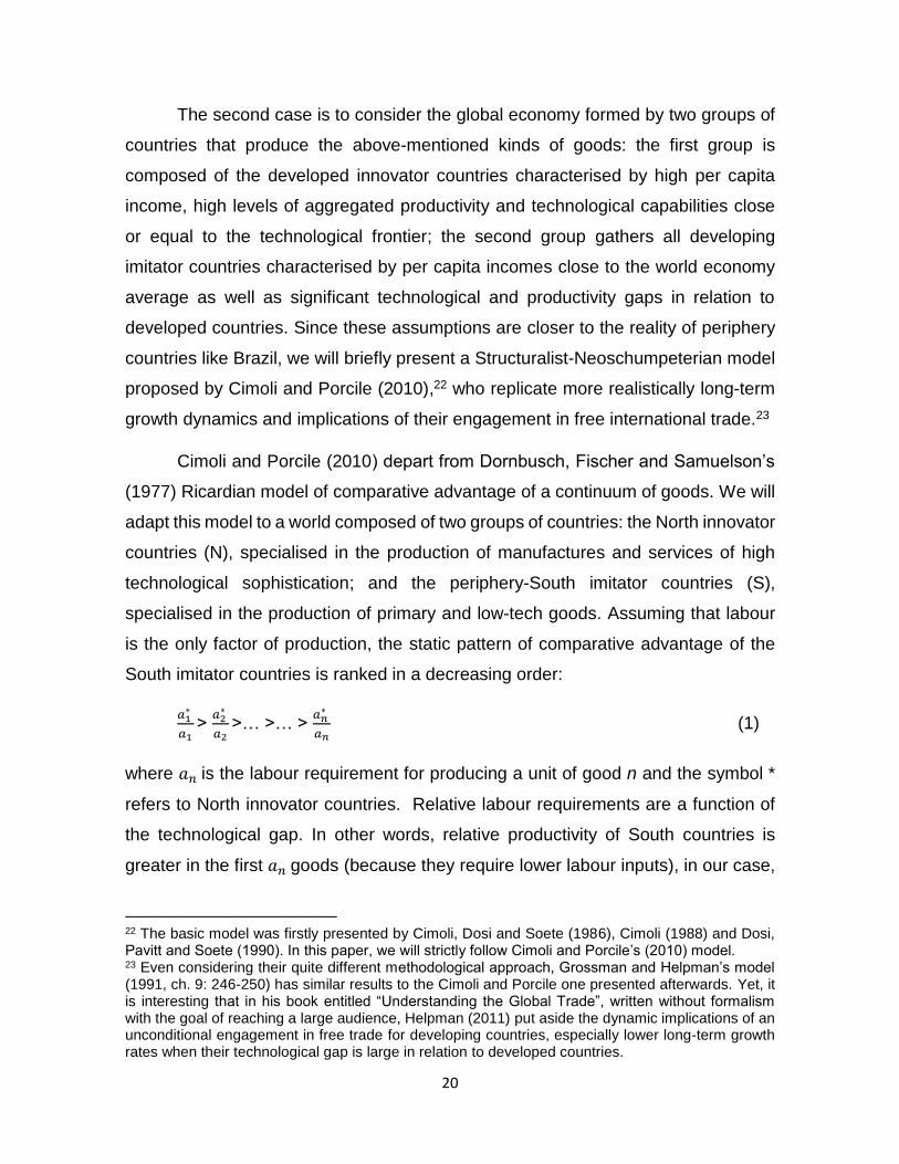
specialised in the production of primary and low-tech goods. Assuming that labour

is the only factor of production, the static pattern of comparative advantage of the

South imitator countries is ranked in a decreasing order:

𝑎1 ∗

𝑎1>

𝑎2 ∗

𝑎2>… >… >

𝑎𝑛 ∗

𝑎𝑛 (1)

where 𝑎𝑛 is the labour requirement for producing a unit of good n and the symbol *

refers to North innovator countries. Relative labour requirements are a function of

the technological gap. In other words, relative productivity of South countries is

greater in the first 𝑎𝑛 goods (because they require lower labour inputs), in our case,

22 The basic model was firstly presented by Cimoli, Dosi and Soete (1986), Cimoli (1988) and Dosi, Pavitt and Soete (1990). In this paper, we will strictly follow Cimoli and Porcile’s (2010) model. 23 Even considering their quite different methodological approach, Grossman and Helpman’s model (1991, ch. 9: 246-250) has similar results to the Cimoli and Porcile one presented afterwards. Yet, it is interesting that in his book entitled “Understanding the Global Trade”, written without formalism with the goal of reaching a large audience, Helpman (2011) put aside the dynamic implications of an unconditional engagement in free trade for developing countries, especially lower long-term growth rates when their technological gap is large in relation to developed countries.

21

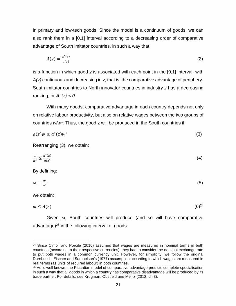
in primary and low-tech goods. Since the model is a continuum of goods, we can

also rank them in a [0,1] interval according to a decreasing order of comparative

advantage of South imitator countries, in such a way that:

𝐴(𝑧) =𝑎∗(𝑧)

𝑎(𝑧) (2)

is a function in which good z is associated with each point in the [0,1] interval, with

A(z) continuous and decreasing in z; that is, the comparative advantage of periphery-

South imitator countries to North innovator countries in industry z has a decreasing

ranking, or A’ (z) < 0.

With many goods, comparative advantage in each country depends not only

on relative labour productivity, but also on relative wages between the two groups of

countries w/w*. Thus, the good z will be produced in the South countries if:

𝑎(𝑧)𝑤 ≤ 𝑎∗(𝑧)𝑤∗ (3)

Rearranging (3), we obtain:

𝑤

𝑤∗ ≤𝑎∗(𝑧)

𝑎(𝑧) (4)

By defining:

𝜔 ≡𝑤

𝑤∗ (5)

we obtain:

𝜔 ≤ 𝐴(𝑧) (6)24

Given 𝜔, South countries will produce (and so will have comparative

advantage)25 in the following interval of goods:

24 Since Cimoli and Porcile (2010) assumed that wages are measured in nominal terms in both countries (according to their respective currencies), they had to consider the nominal exchange rate to put both wages in a common currency unit. However, for simplicity, we follow the original Dornbusch, Fischer and Samuelson’s (1977) assumption according to which wages are measured in real terms (as units of required labour) in both countries. 25 As is well known, the Ricardian model of comparative advantage predicts complete specialisation in such a way that all goods in which a country has comparative disadvantage will be produced by its trade partner. For details, see Krugman, Obstfeld and Melitz (2012, ch.3).

22

0 ≤ 𝑧 ≤ 𝑧(̃𝜔) (7)

Taking (6) as an equality, we can define the border for good z as:

�̃� = 𝐴−1(𝜔) (8)

As 𝐴−1 is an inverse function of A ( 𝜔), the pattern of specialisation of North

innovator countries will be concentrated in the interval:

�̃�(𝜔) ≤ 𝑧 ≤ 1 (9)

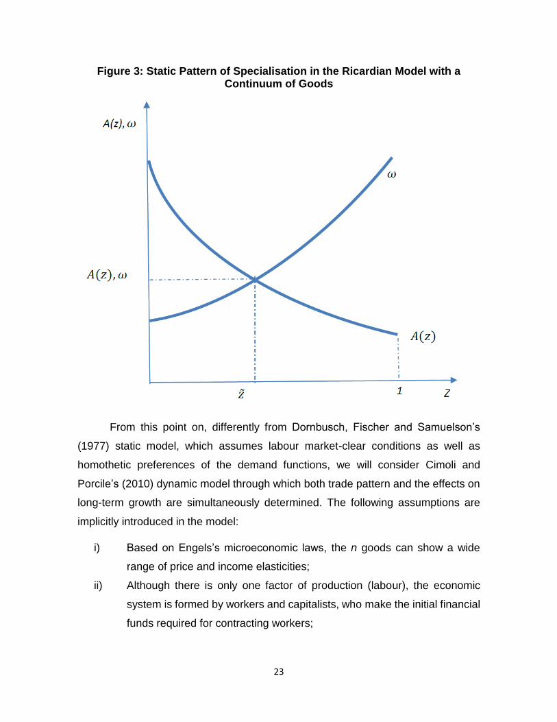
Figure 3 shows the structure of production and pattern of specialisation as a

decreasing function of 𝜔, the relative wage between South and North countries. A(z)

is a decreasing curve because South countries lose comparative advantage as the

economy moves towards goods of higher technological sophistication. Yet, 𝜔 is an

increasing curve in z because as the South countries tend to diversify their

economies, the rise in demand for labour implies an increasing of 𝜔. Figure 3

suggests that an increase in wages in South countries relative to those in North

countries will reduce the set of goods produced and exported by the former group of

countries.26 Under conditions of perfect competition, comparative advantage

depends simultaneously on relative productivities and relative wages between the

two groups of countries. In such circumstances, South imitator countries will have

comparative advantages in all goods for which A(z) > 𝜔. In the world trade

equilibrium, their production and export structures cover all goods from 0 to �̃�, while

the North innovator countries’ ones cover the goods from �̃� to 1.27

26 In a comment on this result, Dosi, Pavitt and Soete (1990: 202) remind us that “it also applies in those cases where there are capital inputs and positive profits, provided that there is no ‘reswitching of commodities’”. 27 Note that at the borderline �̃�, as comparative advantage is the same for all groups, there is no international trade for this good.

23

Figure 3: Static Pattern of Specialisation in the Ricardian Model with a Continuum of Goods

From this point on, differently from Dornbusch, Fischer and Samuelson’s

(1977) static model, which assumes labour market-clear conditions as well as

homothetic preferences of the demand functions, we will consider Cimoli and

Porcile’s (2010) dynamic model through which both trade pattern and the effects on

long-term growth are simultaneously determined. The following assumptions are

implicitly introduced in the model:

i) Based on Engels’s microeconomic laws, the n goods can show a wide

range of price and income elasticities;

ii) Although there is only one factor of production (labour), the economic

system is formed by workers and capitalists, who make the initial financial

funds required for contracting workers;

24

iii) All goods are produced under conditions of imperfect competition, in such

a way that the entrepreneurs fix prices according to a mark-up m on

average labour costs. Thus, the set of goods z will be produced in South

imitator countries if mwaz < m*w* a*z;

iv) Since perfect competition is also removed from labour markets, the

nominal wage is the result of bargaining between labour unions and

entrepreneurs;

v) Rather than labour constrained, capitalist economies are balance-of-

payments constrained in the long run;

vi) Given the state of technology, capitalist economies are generally below

full employment; in the short run, economic activity depends on effective

demand in the spirit of Keynes (1936);

vii) In the long run, changes in technology are endogenously determined and

affected by expected demand.28

By allying with the Structuralist view pioneeringly exposed by Raúl Prebisch

(1950), Nicholas Kaldor (1966) and A.P. Thirwall (1979), Cimoli and Porcile (2010)

present a model in which not only the pattern of specialisation, but also the pace of

long-term growth are affected by the technological gap (TG), defined as the relative

technological levels in North innovator (TN) and South imitator (TS) countries, or29,30:

𝑇𝐺 =𝑇𝑁

𝑇𝑆≥ 1 (9a)

The dynamics of the technological gap is expressed by the following differential

equation (the symbol ^ means change over time):

𝑇�̂� =𝑑(

𝑇𝑁𝑇𝑆

)𝑇𝑆

𝑑𝑡

𝑇𝑆

𝑇𝑁= 𝑎 − 𝑐𝑇𝐺 − 𝑏𝑧 (10)

28 Dosi, Pavitt and Soete (1990: 203), for instance, discard the possibility that technical progress can result from properties related to the steady-state equilibrium with “representative agents” and expectations according to “rational expectations”. 29 Most empirical studies used to take the relative average labour productivity between South and North countries as a proxy measure of the technological gap. In such cases, technological gap TG varies in the interval 0≤G≤1, as we will consider in the empirical section ahead. 30 The remainder of this section rigorously follows Cimoli and Porcile (2010).

25

The differential equation (10) suggests that the pace of the technological gap

between South and North countries is influenced by the actual technological gap

level itself (TG) and the degree of diversification of the economy, captured by the z

produced goods. The parameter a is the autonomous component of the pace of the

technological gap and is expected to be positive. While the parameter b captures

the ability of South countries to imitate innovation (both in process and products)

introduced by North countries, the parameter c represents the opportunities and

challenges posed by the actual technological gap at any time. While the expected

sign of parameter b is positive (the more diversified the economy in producing z

goods, the more rapid the South will catch up with North countries), the expected

sign of parameter c is twofold: in line with Gerschenkron’s (1962) hypothesis, a

positive c means that there are larger opportunities and challenges for South

countries to reduce the technological backwardness in relation to North countries

over time; however, contrary to Gerschenkron’s hypothesis, a negative c, by

meaning a sharp deterioration of relative technological levels, could imply the

deepening of technological backwardness of South countries over time and make it

harder to catch up.

The pattern of specialisation of the economy is also affected by the

technological gap according the following equation (Cimoli and Porcile, 2010: 223):

𝑎∗(𝑧)

𝑎(𝑧)= 𝐴(𝑧) = 𝛾 − 𝛼𝑇𝐺 − 𝛽𝑧 (11)

where 𝛾, 𝛼 and 𝛽 are positive parameters. This implies that if South countries are

successful in reducing their relative technological gap, the curve A(z) in Figure 3

would be shifted to the right, meaning more diversification of South imitator countries

towards a growing number of produced z goods.

To determine the growth dynamics in both groups, Cimoli and Porcile’s (2010)

model assumes no capital flows, in such a way that the current account in North and

South countries must be in equilibrium. Since prices are formed by a mark-up rule

(pz=mwaz=mwLz/yz; where p is the price of good z, m the mark-up, w the wage, az

the labour requirement for producing a unit of good z, L the total labour force, and Y

26

the nominal income related to each good z), total nominal income of South countries

can be expressed as (and, symmetrically, total nominal income in North countries is

related to the production of goods 1 - �̃�):

∫ 𝑚𝑤𝐿𝑧𝑑𝑧 = 𝑚𝑤 ∫ 𝐿𝑧𝑧=𝑧

𝑧=0

𝑧=𝑧

𝑧=0𝑑𝑧 = 𝑚𝑤𝐿 (12)31

The current account equilibrium can be derived from the import demand

functions in each group of countries (that is, the demand of North countries

corresponds to South exports and vice-versa). If each good z has the same share in

total nominal demand in North and South countries, the share of imports in total

demand of the North and South will be, respectively, (w*m*L*)�̃� and (wmL) (1 - �̃�).32

Then, by combining these expressions, the conditions for current account

equilibrium can be expressed as:

𝑚𝑤𝐿 = (𝑧

1−𝑧)𝑚∗𝑤∗𝐿∗ (13)

The relative South-North aggregate income YS/YN can be expressed as a

function of the pattern of specialisation:

𝑌𝑠

𝑌𝑁=

𝑚𝑤𝐿

𝑚∗𝑤∗𝐿∗ =𝑧

1−𝑧 ( 14)

If m = m* and by rearranging (14), we can express the relative wage w/w* as

a function of relative production structures and employment levels:

𝑤

𝑤∗= (

𝑧

1−�̃�)

𝐿∗

𝐿 (15)

By differentiating equation (14) with relation to time, we can obtain the long-

term relative economic growth of the South countries:

𝑌�̇�

𝑌𝑁=

�̇̌�

(1−𝑧)̃2 (16)

31 The nominal income in production of each good z is defined as pzyz=mwLz. In the aggregation, Cimoli and Porcile (2010: 228) assume that m and w are the same in all economies. 32 Remember that while the South produces all goods from 0 to �̃�, the North produces all those from

�̃� to 1 (or 1 - �̃�).

27

By multiplying and dividing the previous result by 𝑧𝑒, we obtain:

𝑌𝑠

𝑌𝑁=

1

1−𝑧(

�̇�

𝑧

𝑧

(1−𝑧) (17)

Expressing 𝑌𝑠

𝑌𝑁= 𝑧 ̃/(1 -𝑧 ̃) and dividing both sides of (17) by

𝑌𝑠

𝑌𝑁 , we find the

long-term relative economic growth rate of South countries:

𝑌�̂�

𝑌𝑁=

�̂�

(1−𝑧)̃ (18)

Equation (18) shows that the technological gap is reduced in South imitator

countries if and only if this group is successful in diversifying its productive structure.

This occurs when �̂� > 0 and South countries can grow at greater rates than North

countries.

The more interesting part of Cimoli and Porcile’s (2010) technological gap

model is when they consider a more realistic case in which goods z have different

income elasticities of demand. The demand function expressed in equation (13) is

replaced by another in which the share of goods in total expenditure rises

exponentially with the number of goods z. Equation (13), the condition for current

account equilibrium in North and South (and remembering that South countries

produce goods from 0 to �̃�), is replaced by:

(𝑚𝑤𝐿)1−𝑧 = (𝑚∗𝑤∗𝐿∗)𝑧 (19)

Expressing (19) in logarithms and differentiating both sides with respect to

time (assuming m and m* are constants), we obtain the dynamic condition for the

current account equilibrium:

−�̇̃� ln(𝑚𝑤𝐿) + (1 − �̃�)(�̂� + �̂�) = �̇̃� ln(𝑚∗𝑤∗𝐿∗) + �̃�(�̂�∗ + �̂�∗) (20)

As in equilibrium z = 0 and, therefore, z = �̃�, we finally obtain the long-term

dynamic growth rate of South countries relative to North ones:

28

�̂�𝑠

𝑌𝑁=

�̂�+�̂�

�̂�∗+�̂�∗=

𝑧

1−𝑧 (21)

With such different specifications for demand functions in both countries, the

result shown in equation (21) suggests two important conclusions: (i) the relative

growth rate of South countries depends on their ability to diversify their economies,

in such a way they will only be able to catch up with North countries if �̃� > 1/2.; and

(ii) since �̃� can also be interpreted as the income elasticity of demand for South

exports (𝜀𝑋), and (1 - �̃�) as the income elasticity of demand for South imports (𝜋𝑀),

equation (21) can be also be translated into the following expression:

�̂�𝑠

𝑌𝑁=

𝜀𝑋

𝜋𝑀 (22)

Equation (22) shows the so-called balance-of-payments constrained growth

rate condition required by Thirlwall’s law: the capacity of South countries to show

growth rates aligned with their balance-of-payment equilibrium over time depends

on the elasticity of demand for their exports being greater than elasticity of demand

for their imports (see Thirlwall, 1979). If so, the South entered a catching up

trajectory; if not, it entered a falling behind path. As Cimoli and Porcile (2010: 232)

conclude:

“The key role of demand growth is highlighted by this result. In effect,

depending on how the demand function is defined, we have very different

implications for economic growth with the same technological gap and pattern

of specialization. The pattern of specialization is endogenous, supply-side

(i.e. technology and productive structure) driven, but the demand functions

define how a specific pattern translates into economic growth. At the end of

the day, both the Schumpeterian and Keynesian sides of the growth equation

must be taken into account in the model.”

29

3. Empirical evidence: the case of Brazil

In this section, we will analyze the evolution of the trade patterns of the

Brazilian economy between 1990 and 2016. Throughout this period, Brazil

experienced a process of trade liberalisation (1990-1994), the stabilisation of high

inflation rates (Plano Real, 1994) and other liberalising economic reforms, such as

privatisation of state enterprises, the liberalisation of the domestic financial system

and the openness of the capital account, among others. This section is divided into

two subsections: in the first, we will briefly analyse the main reforms introduced in

Brazil in this period, with emphasis on trade liberalisation; in the second, we will

show empirical evidence on the changes that occurred in the Brazilian trade

patterns.

3.1. A brief analysis on Brazil’s economic reforms and some previous

indicators (1990-2017)

From the last quarter of the nineteenth century to 1930, the Brazilian economy

was highly open to international trade and, despite the presence of a few infant low-

tech industries, unable to show a vigorous industrialisation process. In this period,

Brazilian productive and export structures were strongly concentrated on coffee and

other primary products of low income and price-elasticity of demand. By depending

on the export performance of these goods in the global markets, long-term economic

growth in Brazil was driven by world markets and constrained by price volatility of its

main exports. At the same time, in the absence of a vigorous manufacturing sector,

a significant share of manufactured goods was imported (Furtado, 1959).

The dramatic crisis of the Brazilian primary export sector resulting from the

Great Depression of the 1930s put an end to the previous development model and

was responsible for the spontaneous process of industrialisation based on import

substitution (IS).33 From the 1930s on, Brazil’s long-term growth has been driven by

the dynamism of the domestic market. However, the process of industrialisation only

gained momentum after 1950, especially under Getúlio Vargas’s second-term

33 Furtado (1959).

30

(1950–1954) and Juscelino Kubistschek’s (1956–1960) government, which adopted

several protectionist measures in favour of infant heavy industries.34

From the mid-1950s to the beginning of the 1980s, industrial and trade

policies maintained their essential elements. In each step of the IS process,

governments targeted some industries as priorities of the industrial policy and

combined high tariffs, import licenses and export subsidies (these latter especially

after the 1970s) to protect the Brazilian manufacturing sector and boost exports of

manufactured goods. In practice, the import license regime was only eliminated with

trade liberalisation in March 1990.35 Even considering the two attempts at trade

liberalisation in 1966 and 1988, the economy maintained a very high protectionist

structure—at least when compared to that adopted by the Asian Tigers at the height

of their protectionist policies36—due to the prevalence of non-tariff barriers (NTB).37

Another peculiarity of the industrial policy in Brazil is related to foreign direct

investment (FDI), which has always been open to multinational enterprises (MNE).

Policies for attracting MNEs in Brazil focused on the implemention of import

substitution and, hence, the reduction of both technology and import dependencies

(balance of payments issues). This is in contrast to some Asian countries that were

traditionally open to FDI, such as Singapore and China. These countries included

measures that ensured the transfer of technology or technological spillovers to local

firms. Therefore, Brazil was not able to draw upon the best techniques available in

important industries of high and even medium technologies, such as capital goods,

and chemical and automotive industries (Dahlman and Frischtak 1993).38

Although the protectionist policies have been marked by several drawbacks,

such as the absence of selectivity, an obsession with national content and the

34 Tavares (1963). 35 An import license as a sine qua non condition for an import to be approved lasted from 1947 to 1970, when the former was replaced by the “guia de importação” (an import document issued by the Foreign Trade Department, Cacex). Although the creation of this document has been justified for fulfilling statistical purposes, in practical terms it continued to work as an instrument of administrative import control. See Nassif (1995). 36 See Amsden (2001). 37 Nassif (1995). 38 As Amsden (2001:14) commented, “China, India, South Korea and Taiwan began to invest heavily in their own proprietary national skills. In contrast, Argentina and Mexico, and to a lesser extent, Brazil and Turkey increased their dependence for future growth on foreign know-how”.

31

survival of rent-seeking activities, in the period 1957-1980, there was a fine

coordination between industrial and trade policies, in such a way that the latter was

conditioned by the main goals of the several adopted National Development Plans.

Despite all the imperfections of the protectionist policies of the IS period, there is no

doubt that they created the conditions for developing a diversified manufacturing

sector in Brazil over time.39

It is important to stress that, differently from some Asian countries (e.g. China

and Taiwan), which sought to finance a significant share of gross investment with

domestic savings, Brazil’s development strategies were highly dependent on foreign

savings, especially through long-term foreign lending, which, borrowed under

conditions of flexible international interest rates, was the main modality observed

from the 1970s on. The shock of international interest rates in the 1979-1982 period

led Brazil and several other Latin American countries to a deep crisis (the external

debt crisis) that lasted until the beginning of the following decade.

In fact, the eruption of the external debt crisis in 1980, which led to the

collapse in international private capital flows to Latin American countries in 1982,

meant a complete disconnection between industrial and trade policies as strategic

mechanisms for promoting catching up in Brazil. In the face of a large amount of

annual services (principal and interest expenditures) on external debt, trade policies,

especially import policy, became a powerful instrument for controlling foreign

exchanges. The most infamous instrument for import control was the so-called

Annex C, released by Brazil’s Foreign Trade Department (CACEX), through which

thousands of goods were prohibited in Brazil between 1980 and March 1990. In

1984, manufactured goods included in Annex C represented 46.8% of total goods

registered in the old Brazilian Merchandise Nomenclature (NBM) and 10.5% of total

Brazilian imports. In 1989, several goods of textile & clothing, footwear, plastic and

motor vehicle industries still had import prohibition (Carvalho Jr., 1992). In practice,

the long duration of such import control virtually meant infinite protection for the

respective domestic industries.

39 For a comparison between interventionist policies and the process of industrialisation in Brazil and South Korea, see Moreira (1995).

32

The decision to introduce a unilateral trade liberalisation reform in Brazil

between March 1990 and 1994 must be understood within this economic context. In

such circumstances, the programme was designed with the goal of redesigning the

structure of protection through the elimination of most non-trade barriers (NTBs),

including the Annex C, as well as the reestablishment of the import tariff as the main

instrument of protection for the economy. Comparatively to other experiences of

trade liberalisation in developing countries during the 1980s and the 1990s, the

Brazilian trade reform represented a deep microeconomic shock for three reasons:

first, it was concluded in a relatively rapid period of time (5 years), differently from

South Korea and India, whose trade liberalisation reforms lasted around 6 (from

1983 to 1988) and more than 10 years (from 1991 on) , respectively;40 second,

contrary to the recommendations of trade liberalisation literature, the elimination of

NTBs and reduction of import tariffs were jointly introduced, and trade reform was

adopted together with the liberalisation of capital account as well as within a context

of sharp overvaluation of the Brazilian currency;41,42 and third, again, differently from

South Korea and India, which preserved industrial policy together with their trade

liberalisation programmes as a strategy for pursuing catching up, industrial policy

practically disappeared from the government’s policy focus in Brazil between 1990

and early 2000s, even after the conclusion of trade reform.43

40 Between 1989 and 1994, while the average nominal import tariff for all goods in Brazil was reduced from 39.6% to 11.2%, the standard deviation dropped from 14.6% to 5.9% in the same period. See Kume, Piani and Souza (2000:11). 41 For Brazil and South Korea, see Moreira (1995). For India, see Nassif (2003; 2007). 42 For a theoretical discussion on how the speed and sequence of trade liberalisation reforms should be designed, based on stylised facts of real experiences in Latin America and Asia, see Bhagwati (1978) and Michaely, Papageorgiu and Choski (1991). For the order of overall economic liberalisation, see McKinnon (1991). 43 In the case of South Korea, the clear change in priorities did not mean discarding industrial policy to promote structural change. According to the OECD (2012), “since the 1980s, the government carried out research and development (R&D) and gave incentives to the private sector for investing in R&D. By the 1990s, the chaebols (Korean conglomerates), were highly committed to R&D and the government widened the policy mix for R&D to include support to venture business in line with the rising demand from the private sector”. The OECD (2012: 24) also documents that, by 2011, the Korean government maintained industrial promotion programmes for “leading industries”, “strategic industries” and “infrastructure and business support”. Yet India’s governments never renounced industrial policy, which continued to be included in the 5-Year Plans after trade liberalisation in 1991 (see Nassif, 2007).

33

These aspects refer to the negative microeconomic shocks represented by

trade liberalisation in Brazil. However, several studies show sound empirical

evidence that between 1990 and 1998 labour productivity registered significant

annual average growth rates in Brazil, reversing the low and stagnant annual

average growth rates shown in the previous decade. In a panel data econometric

model based on industrial plants, Nassif (2005), for instance, estimated that labour

productivity in the manufacturing sector grew at 1.4% between 1988 and 1994, and

5% between 1994 and 1998. These results confirm similar empirical evidence of

previous studies, which had also attributed such performance to the positive impacts

of the Brazilian trade liberalisation.44

Table 1 gives an updated tariff structure for Brazil compared with other

selected countries.

Table 1: Tariff structure in selected countries (in percentage)

Two conclusions can be drawn from Table 1. First, by comparing with some

developing and developed countries, it is a myth to assert that Brazil is still very close

to being or is a protectionist country. The simple average tariff rate applied to all

products (11.6%) in 2017 was lower than that of South Korea (14.1%) and India

44 See Hay (1997), Bonelli and Fonseca (1998), Rossi Jr. and Ferreira (1999), and Bonelli (2002).

Brazil (2017) Russia (2016) India (2015) China (2015) South Africa* (2015) South Korea (2016)

Simple average tariff rate 11.6 8.3 13.0 9.5 8.3 14.1

WTO agricultural products 10.2 14.6 36.4 14.8 9.9 60.0

WTO non-agricultural products 11.8 6.5 9.5 8.6 8.0 6.6

Bound tariff lines (% of all tariff lines) 100 100 74.9 100 n.a. 90.1

Tariff quotas (% of all tariff lines) 0.4 0.4 n.a. 0.6 n.a. 1.9

Non-ad valorem tariffs (% of all tariff lines) 0.0 14.8 6.1 0.5 3.8 0.8

International tariff peaks (% of all tariff lines) 27.0 6.4 13.6 14.8 21.4 10.7

Minimum tariff for all applied tariff rates 1 0.0 0.0 0.0 0.0 0.0 0.0

Median tariff for all applied tariff rates 1 14.0 5.0 10.0 8.0 n.a. 8.0

Maximum tariff for all applied tariff rates 1 41.3 80.0 150.0 65.0 55.0 800.3

Overall standard deviation of all applied tariff rates 8.4 1 10.3 16.5 7.5 14.1 44.1 1

Notes: * refers to Southern African Custom Union; 1: Data for 2014, calculated by Castilho and Miranda (2017); n.a.: not available

Source: World Trade Organization, Trade Policy Review, Several Issues.

34

(13.0%). The degree of dispersion of all applied tariff rates, measured by the

standard deviation, is one of the lowest among the BRICS countries (Brazil, Russia,

India, China and South Africa) and much lower than South Korea, whose indicator

was 44.1% in 2016. These results do not match with Bonelli’s (2015: 487, translated

from Portuguese) assertion, according to which “Brazil is an economy with very few

links to the international economy”. In a similar line, Bacha (2016: 3, translated from

Portuguese) comments that “Brazil is one of the most closed economies in the

world”. It is true that, by 2016, the share of trade flows (exports plus imports) in

Brazil’s GDP (18.3%) was very low compared with middle income countries (38.6%)

or countries like India (27.5%), whose economy is more protected than Brazil, as

Table 1 shows. However, Brazil’s low degree of trade openness can be explained

by the lack of competitiveness of manufacturing exports as well as the very low

annual GDP growth rates (which imply low import volumes) observed in the last

decades (only 2.4% between 1999 and 2016).45 In addition, it is well known that

continental economies such as the United States, Australia and Indonesia are more

closed than small economies. These countries usually have a large domestic market

and a quite diversified productive structure.

Second, although the use of the international peaks covers a significant part

of all tariff lines,46 such peaks are in line with the Most Favourable Nation (MFN)

tariffs negotiated multilaterally at the WTO. In any event, Brazilian effective tariff

rates estimated by Castilho and Miranda (2017) for 2014 (an average rate of 16.7%

and a standard deviation of 15.2% for the overall economy) suggest that the

structure of protection in Brazil should be redefined with the goal of reducing the very

high level of protection of sectors like buses and trucks (72.5%), automobiles

45 The problem of the lack of competitiveness of exports will be discussed in the next subsection. Indicators on share of trade flows in GDP were drawn from the World Bank, World Economic Indicators. https://data.worldbank.org/indicator/TG.VAL.TOTL.GD.ZS. Accessed on 13 October 2017. Indicators on Brazil’s annual GDP growth rates were drawn from the Brazilian Institute of Geography and Trade (IBGE), Quarterly National Accounts at 1995 constant prices. https://sidra.ibge.gov.br/pesquisa/cnt/tabelas. Accessed on 13 October 2017. 46 Moreover, for the WTO, tariff peaks correspond to rates exceeding 15%. Other possible definitions take into account the tariff level and structure of the country. For instance, Castilho and Carvalho (2017) consider tariff peaks as the rates that exceed the sum of the tariff average and the standard deviation.

35

(65.5%), clothing (39.9%), textiles (30.3%) and household appliances (26.4%) as

well as several intermediate goods of chemicals and related products (around 20%).

From 2003 on, especially during Lula da Silva’s (2003-2010) and Dilma

Rousseff’s governments (2011-2014), industrial policy returned as one of the leading

mechanisms for promoting activities considered strategic for accelerating structural

change towards scale-engineering-and-knowledge-based industries as well as

diversifying productive and export structures, such as capital goods, software,

information and communication technologies, pharmaceutical products,

biotechnology, automobiles and others. In this period, three programmes of

industrial policy were announced: Foreign Trade, Technological and Industrial Policy

(PITCE, in Portuguese), in 2004; the Production Development Policy (PDP), in 2008;

and Largest Brazil Plan (Plano Brasil Maior, in Portuguese – PBM), in 2011.47 All

these plans had as their core goal to boost physical investment and innovation in the

Brazilian economy.

The trouble with all these plans is that they repeated old mistakes and well-

known misleading policies that had prevailed during the time of the import

substitution period: lack of selectivity and performance requirements from

entrepreneurs who benefited from public incentives; an excessive use of public

subsidies as the main instrument of governmental support, especially credit

subsidies from the Brazilian Development Bank (BNDES); and, last but not least,

total lack of coordination between industrial, trade and macroeconomic policies. One

example of coordination failure is related to the recurrent trend of overvaluation of

the Brazilian real. Figure 4 plots the behaviour of the real effective exchange rate

(REER) in Brazil since 1988.48

47 For an analysis of PITCE and PDP industrial policies, see Coutinho et al. (2012). For details on Plano Brasil Maior, see the website of Brazil’s Ministry of Development, Industry and Commerce (MDIC), http://www.mdic.gov.br/index.php/competitividade-industrial/politica-industrial/o-que-e-pbm-2 . Accessed on 12 October 2017. 48 In Brazil, the exchange rate is defined as the domestic price of a foreign currency. So, while an increase in the exchange rate means a depreciation of the Brazilian real, a decrease means an appreciation of it. The real effective exchange rate was calculated by the Central Bank as a weighted average of the Brazilian real against a basket of currencies of Brazil’s main trade partners, adjusted by the consumer inflation rate (IPCA).

36

Figure 4: Brazil: real effective exchange rate (REER) – 1988 to August, 2017 (Index-base = Jun-1994=100)

Source: Brazil’s Central Bank

Figure 4 shows unequivocally that the overvaluation of the Brazilian real has

been a recurrent trend since the early 1990s. The correction of such misalignments

has only occurred after domestic or international shocks, such as the announcement

of the stabilising Real Plan (Plano Real) in June 1994, the crisis of the electrical

energy sector (apagão) in 2001, the electoral uncertainty during the transition from

the presidency of Fernando Henrique Cardoso to Luiz Inacio Lula da Silva in 2002-

2003, the aftermath of the 2008 global crisis and, finally, during the instability created

by the impeachment of president Dilma Rousseff throughout 2015. After all these

episodes, the Brazilian real has entered a new appreciation trend in real terms. In

an econometric model seeking to identify the main forces that pushed the Brazilian

real towards that appreciation trend in the period 1999-2015, Nassif, Feijó and

Araújo (2017) showed that both the favourable terms of trade and the sharp

differential between Brazilian and international interest rates were the most

significant explanatory variables.

37

Several studies have shown a strong correlation between the trend of

overvaluation of the Brazilian real and the weak long-term economic performance of

the Brazilian economy, expressed by a sharp premature deindustrialisation49 as well

as low rates of productivity and economic growth. After having been positively

impacted by trade liberalisation between 1988 and 1998, as previously discussed,

the annual average growth rate of labour productivity in the Brazilian manufacturing

sector has been stagnant and showed negative results between 1999 and 2015 (-

0.2% p.y.).50 With such a stagnant performance, it is not surprising to verify,

according to Figure 5, that the technological gap of the manufacturing sector in Brazil

(measured as the ratio of Brazil’s labour productivity to the U.S. labour productivity),

after having shown a slow catching up trajectory between 1970 and 1980, has

tendentially widened outwards, as can be seen by the trend line.51 Figure 5 also

shows that the last period during which all segments of the Brazilian manufacturing

sector significantly reduced the technological gap occurred in the aftermath of trade

liberalisation, especially between 1990 and 1998, as we discussed earlier.

Particularly, the science-engineering-and-knowledge-based industries, after having

reached almost half of the technological frontier in 1997, entered a falling behind

trajectory afterwards. Although these indicators have not been updated by ECLAC-

PADI, such trends can hardly have registered significant changes in the opposite

direction, in the face of the stagnant behaviour of the labour productivity growth in

the manufacturing sector in Brazil in the last decade, as we commented earlier.

49 Several studies have attributed the real appreciation trend of the Brazilian currency as being one of the main causes of Brazil’s premature deindustrialisation. See, for instance, Bacha (2013), Bresser-Pereira (2010), Nassif, Feijó and Araújo (2015) and Nassif, Bresser-Pereira and Feijó (2017). 50 These results were calculated and kindly offered to the authors by Jorge N.P. Britto, from the Department of Economics at the Fluminense Federal University. The labour productivity was calculated as the ratio of the value of industrial transformation (a proxy for value added) to the number of employees directly occupied at production (these indicators are estimated, in turn, by the Annual Industrial Survey – PIA, from the Brazilian Institute of Geography and Statistics - IBGE). The numerator was deflated by sectoral Wholesale Price Indices (IPA) of Fundação Getúlio Vargas. 51 These data are estimated by the Program for the Analysis of Industrial Dynamics (PADI) of the United Nations Economic Commission for Latin America and the Caribbean (ECLAC).

38

Figure 5: Technological gap in the Brazilian industries of the manufacturing sector classified by factor content and technological sophistication

Source: ECLAC-PADI

The falling behind trajectory of the Brazilian economy can also be confirmed

by the results of Thirlwall’s law for the Brazilian economy between 1980 and 2010—

see equation (22) in Section 2—, estimated by one of the authors in a previous paper

(see Nassif, Feijó and Araújo, 2015), and summarised in Table 2.

39

Table 2: Thirlwall’s law and the falling behind trajectory of the Brazilian economy (1980-2010)

Note: 1, 2, 3 and 4 refer to quarters. Source: Nassif, Feijó and Araújo (2015: 1326)

According to Table 2, while between 1980 and 1998, Brazil’s estimated

annual average growth rate compatible with its balance of payments equilibrium was

69% lower than the world GDP growth rate, between 1999 and 2010, this rate

reduced significantly to only 39.5%, confirming the falling behind path in the

decade.52

3.2 Brazil’s trade patterns and the recent trajectory towards regressive

specialisation

For Brazilian international trade, the period comprised between 1990 and

2016 was characterised by a strong dynamism. During these 26 years, the total

trade value was multiplied by 6 while world trade was multiplied by 4. Brazilian

exports attained US$336 billion and imports, US$246 billion.

The performance of Brazilian international trade was nevertheless very

different during the 1990s and the 2000s. As shown in Figure 6, not only was the

growth in trade flows stronger in the 2000s but also the dynamics of exports and

imports were opposite in the two periods. During the 1990s, after the Brazilian trade

52 In another paper (Nassif, Feijó and Araújo, 2016), we estimated Thirlwall’s law for all the BRICS (Brazil, Russia, India, China and South Africa) in the period 1995-2013. The results did not alter for Brazil and revealed that only China and India showed a catching up trajectory in the period.

40

liberalisation and the overvaluation of Brazil’s currency, imports grew at a faster pace

than exports. From the 2000s on, Brazilian exports grew faster than imports, even

though imports also increased significantly.

The Brazilian market share (total trade) evolved from 0.8% of world trade in

1990 to 1.4% in 2016.53 During the 1990s, the Brazilian market share increase was

pulled by the significant expansion of imports. The cumulated growth rate of Brazilian

imports (148%) was twice the exports growth rate (75%) and well above the world

trade growth rate (96%). From 2000 on, Brazilian exports grew faster than Brazilian

imports (236% and 147%, respectively) but both of them showed higher rates than

global trade (119%). Therefore, Brazil attained its highest participation in world trade

in this 25-year period for exports in 2011 (1.5%) and for imports in 2013 (1.3%). The

different pace of the recent decrease in world and Brazilian trade flows made the

export market share recover to 1.4% (2016 data).

53 In a longer-term perspective, Brazilian exports attained their highest world market share during the 80s (trade statistics are available from 1962 on). The market share average was 1.3% for the whole decade (lower than the period 2010-2016) but it attained 1.7% in 1984. On the other hand, the lowest average was reached during the 90s, when Brazilian market share was 1.0%. From then on, the share has increased both in the 00s and during the last period (2010-2016).

41

Figure 6: Brazilian exports, imports and market share evolution

(1990-2016)

Source: Elaborated by the authors based on COMTRADE database.

In Table 3, trade flows were broken down according to the relative use of

productive resources (resource-based versus labour intensive) as well as the degree

of technological sophistication according to Pavitt’s (1984) classic taxonomy. The

strong increase in Brazilian trade flows over this period was accompanied by

important composition changes, mainly on the export side. On the import side, the

sectoral composition kept relatively stable, with the manufactured goods

representing a large majority of imports. In the first half of the 1990s, there was an

important reduction in oil imports as a consequence of the increase in the national

production. After that, changes in import structure were minor, with the exception of

the increase in imports of labour and scale intensive sectors.54

54 The increase in labour intensive imports was strongly influenced by the rise in textiles, clothing, shoes and some chemical goods, while the transport equipment imports (cars, trucks and ships) were the main reason for the share of scale intensive goods to increase.

0.0

0.2

0.4

0.6

0.8

1.0

1.2

1.4

1.6

0.0

50.0

100.0

150.0

200.0

250.0

300.0

350.0

400.0

450.0

500.0

19

90

19

91

19

92

19

93

19

94

19

95

19

96

19

97

19

98

19

99

20

00

20

01

20

02

20

03

20

04

20

05

20

06

20

07

20

08

20

09

20

10

20

11

20

12

20

13

20

14

20

15

20

16

Wo

rld

Mar

ket

shar

e -

in %

Ind

ex

: bas

e 2

00

0=

10

0

World imports index Brazil exports index

Brazil imports index Brazil market share - exports

Brazil market share - imports

42

On the export side, as stated, there were important composition changes.

Manufactured goods share in exports remarkably decreased, going from 78% of total

exports in 1990-1995 to 53% in 2011-2016.55 After losing export shares during the

1990s, the share of primary goods doubled and recovered the importance they used

to have in the beginning of the 1970s. This process has been named “export

primarisation” and, as mentioned in section 3.1, several factors explain it, such as

the commodities price boom in the 2000s, the persistent overvaluation of the national

currency and the dynamism of domestic demand for manufactured goods. The

primarisation process observed in exports was not, however, observed—at least not

with the same intensity—in domestic production. In fact, Torracca (2017) shows the

mismatch between the structure of exports and of domestic production. While

primarisation is clear and strong in external trade flows, the domestic production

structure is much more stable and less intensive in primary goods and resource

based sectors, even though their share in domestic production increased. These

conclusions do not contradict the evidence of premature deindustrialisation in Brazil,

especially from the mid-2000s on. However, in Brazil this phenomenon was marked

by a sharp reallocation of resources from the manufacturing sector to segments of

low productivity in the tertiary sector.56

All manufacturing sectors experienced a decrease in their share in total

exports at the beginning of the 1990s, except the science-based group (Table 3).

The reduction in the share of manufactured goods in total Brazilian exports is, in

part, explained by the exceptional increase in primary goods exports.57 In fact,

55 See Bacha and Fishlow (2011), Bacha (2013) and Nassif, Feijó and Araújo (2017). 56 In fact, according to the Brazilian Institute of Geography and Statistics (IBGE), the share of the agricultural sector in Brazil’s GDP in real terms (1995 price) in 2016 was virtually the same as that of 1996 (6%). Yet, while the share of the manufacturing sector in total GDP was reduced from 13.8% to 9.8%, the share of the tertiary sector was increased from 57% to 60.7% during the same period. See https://www.ibge.gov.br/estatisticas-novoportal/economicas/contas-nacionais/9300-contas-nacionais-trimestrais.html?&t=resultados. Accessed on 25 October 2017. See Nassif (2008) for the 1947-2004 period (in current prices). 57 The cumulated growth rate of Brazilian exports exceeded the rate of world exports for manufactured goods for the entire period 1990-2016 due mainly to the good performance between 2004 and 2013. Moreover, as shown by Castilho et al. (2017), the export primarisation in Brazil has a very strong geographical character since exports to China, which became the first trade partner after the financial crisis, are very concentrated in primary and resource based goods.

43

despite their relative contraction in total exports, Brazilian manufactured goods grew

at a faster pace than world exports of manufactured goods.

Table 3: Composition and evolution of Brazilian exports and imports by product groups (1990-2016)

Among manufactures, labour intensive goods are the product group which

lost more participation in exports since 1990 (from 13% to 5%), since the

competitiveness of Brazilian goods in markets which became increasingly

competitive declined. Exports of scale intensive goods also showed a significant

decrease especially due to the reduction of steel products. The exports of science

based goods showed quite a dynamic trajectory till 2005, when their share in total

Primary

goods

Resource

based

industry

(1)

Labour

intensive

(2)

Scale

intensive

(3)

Specialized

suppliers

(4)

Science

based (5)n.d

Manufactured

goods (1-5)Total

1990-1995 21.1 28.5 12.6 23.0 9.7 4.0 1.0 77.9 100.0

1996-2000 22.4 27.3 10.6 21.1 9.8 7.2 1.6 76.0 100.0

2001-2005 26.4 24.2 9.2 20.4 9.1 8.8 1.8 71.8 100.0

2006-2010 36.8 22.3 6.3 17.2 8.1 7.2 2.2 61.1 100.0

2011-2016 45.1 21.2 4.9 14.5 7.2 5.2 1.9 53.0 100.0

1990-1995 5.4 9.7 7.7 8.2 10.7 5.6 10.3 8.2

1996-2000 5.0 (1.9) 2.3 2.3 1.5 29.2 11.4 3.5

2001-2005 23.4 13.9 10.4 18.5 17.7 7.9 15.2 16.5

2006-2010 21.6 11.3 1.6 1.9 4.7 3.5 11.6 11.2

2011-2016 (2.3) (1.3) (0.7) 0.9 (0.1) (1.7) (8.4) (1.4)

1990-1995 20.7 22.5 7.6 14.4 18.8 15.9 0.0 79.3 100.0

1996-2000 12.6 20.5 8.7 16.3 21.8 19.9 0.1 87.2 100.0

2001-2005 15.5 18.5 7.8 14.2 21.3 22.6 0.0 84.5 100.0

2006-2010 14.4 19.3 8.4 17.7 19.0 20.1 1.2 84.4 100.0

2011-2016 11.2 21.0 9.7 19.2 18.7 20.2 0.0 88.7 100.0

1990-1995 (1.3) 25.3 33.2 38.2 19.7 19.1 39.0 19.1

1996-2000 (0.6) (0.9) (3.7) (4.9) 2.5 9.0 48.2 0.7

2001-2005 13.1 2.1 5.5 6.5 4.6 5.0 (48.2) 5.7

2006-2010 10.7 22.3 22.9 27.7 19.6 16.2 105.5 19.7

2011-2016 (7.9) (4.2) (2.6) (6.8) (4.7) (1.6) (2.8) (4.5)

Source: Elaborated by the authors based on COMTRADE database.

Average Annual Growth (p.y.%)

EXPORTS

Composition (% of total exports)

Average Annual Growth (p.y.%)

IMPORTS

Composition (% of total imports)

44

exports began to retract. In 2016, their share (5.6%) was close to the average of the

90s. Finally, despite the loss of around one quarter of their participation in total

exports, resource-based and specialised suppliers were the only categories which

augmented their share in manufacturing goods exports.

The different export performances of the product groups are illustrated with

annual data in Figure 7. While the reduction in the share of scale intensive, labour

intensive and resource based goods began in the first half of the 90s, specialised

suppliers and science based goods performed well for a longer time during the

period 1990-2016. The highest export share of specialised suppliers was attained in

1996 and for science based goods, from 2000.

Figure 7: Evolution of Brazilian exports composition by product groups (1990-2016 – % of total exports)

Source: Elaborated by the authors based on COMTRADE database.

Despite the strong loss of importance of manufactured goods in Brazilian

exports, their performance in world markets is less dramatic. In fact, the so-called

primarisation process is partially explained by the commodities price boom and

2016: 42%

1995: 80,5%

2016: 59%

-

10.0.0

20.0.0

30.0.0

40.0.0

50.0.0

60.0.0

70.0.0

80.0.0

90.0.0

19

90

19

92

19

94

19

96

19

98

20

00

20

02

20

04

20

06

20

08

20

10

20

12

20

14

20

16

Primary goods

Resource based

Labour intensive

Scale Intensive

Spec. Suppliers

Science based

Manuf. goods

45

affected not only Brazil but also world exports. For manufactured goods, we can

observe from Figure 8 that Brazil kept its (low) share of 1% in world exports until

2008. In terms of world market share, the product groups performed very differently.

The labour-intensive goods are the only group presenting a net reduction from 1990

to 2016—a 25% loss of its world market share. Exports in science base goods

increased their share in world exports during the 2000s and decreased from 2009

on, reaching 0.4% at the end of the period. Scale-intensive goods reached their

highest share in world markets in 2005 and after, their participation kept floating

around 1%. Specialised suppliers goods are the group with a more stable share

during the period—around 0.6% over the 25 year period. Finally, resource based

goods, even showing a slightly decreasing tendency between 1995 and 2014, is the

manufacturing sector with the highest share in the world market. Primary goods,

which are not shown in Figure 8, presented a completely different performance: their

market share, after a decade of relative stability of around 1.8% in the 90s, was

multiplied by 3.4 by 2016. Brazilian primary goods exports represented in this year

6.3% of total world exports.

Figure 8: Market share of Brazilian manufacturing exports, by product group (1990-2016, % of world exports)

Source: Elaborated by the authors based on COMTRADE database.

3.8

1.9

1.0

1.3

0.70.7

1.5

1.00.9

0.00

0.50

1.00

1.50

2.00

2.50

3.00

3.50

4.00

Primary goods

Resource based

Labour intensive

Scale Intensive

Spec. Suppliers

Science based

Total

Manufactured goods

46

A traditional indicator of a country’s pattern of specialisation is Balassa’s

(1965) Revealed Comparative Advantage (RCA) [see equation A.1 in Appendix 1],

whose results are shown in Figure 9.58 Indicators clearly register a deepening of

Brazilian export specialisation based on primary goods. Since it was accompanied

by a continuous drop of the RCA of several manufactured goods categories

(notably, labour-intensive, science-based and specialised suppliers), these results

characterise a regressive specialisation of Brazilian trade. Changes were stronger

from 2000 on than over the 1990s.59

Figure 9: Brazilian Revealed Competitive Advantage

Source: Calculated by the authors based on COMTRADE database.

For analysing if, and if so the extent to which, Brazilian trade flows have been

concentrated or diversified in the last decades, we used the Herfindahl-Hirschman

index (HHI) as specified in equation A.2 in Appendix 1 and shown in Figure 10. As

58 If RCA is above 1, that means the country has comparative advantage , whereas if RCA is below

1, that means absence of comparative advantage—or comparative disadvantage. 59 For details, see Nassif, Feijó and Araújo (2015).

0.0

0.5

1.0

1.5

2.0

2.5

3.0

3.5

4.0

4.5

5.0

1990 1995 2000 2005 2010 2015 2016

Primary goods

Resource basedindustry

Labour

intensive

Scale intensive

Specialized

suppliers

Science based.

Manufactured

goods

47

the HHI basically measures the degree of concentration (the larger the HH index,

the more concentrated are the exports or imports), Figure 10 shows that Brazilian

imports are more diversified than exports. The HHI also puts in evidence not only

the difference in the concentration degree of trade flows, but also the divergent

trends in the last ten years. Exports have shown a concentration trend after 2004,

while imports presented a more stable evolution, after the diversification in the first

half of the 1990s. The maximum level of export concentration measured by the HHI

was reached in 2011. This latter result reflects the emergence of China as one of

the most important Brazilian trade partners. In the case of exports to China, they are

very concentrated in mineral ores, soybeans and oil and grew sharply after the 2008

global crisis. 60

Figure 10: Degree of concentration of Brazilian exports and imports (Herfindahl-Hirschman Index, 1990-2016)

Source: Calculated by the authors based on COMTRADE database.

60 These three products represent around 75% of Brazilian exports to China. As international prices of these commodities were very high until 2012, the share of these products in total exports rose remarkably.

0.000

0.010

0.020

0.030

0.040

0.050

0.060

19

90

19

91

19

92

19

93

19

94

19

95

19

96

19

97

19

98

19

99

20

00

20

01

20

02

20

03

20

04

20

05

20

06

20

07

20

08

20

09

20

10

20

11

20

12

20

13

20

14

20

15

20

16

Exports Imports

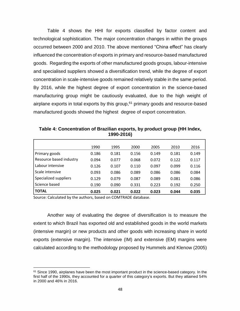
48

Table 4 shows the HHI for exports classified by factor content and

technological sophistication. The major concentration changes in within the groups

occurred between 2000 and 2010. The above mentioned “China effect” has clearly

influenced the concentration of exports in primary and resource-based manufactured

goods. Regarding the exports of other manufactured goods groups, labour-intensive

and specialised suppliers showed a diversification trend, while the degree of export

concentration in scale-intensive goods remained relatively stable in the same period.

By 2016, while the highest degree of export concentration in the science-based

manufacturing group might be cautiously evaluated, due to the high weight of

airplane exports in total exports by this group,61 primary goods and resource-based

manufactured goods showed the highest degree of export concentration.

Table 4: Concentration of Brazilian exports, by product group (HH Index, 1990-2016)

1990 1995 2000 2005 2010 2016

Primary goods 0.186 0.181 0.156 0.149 0.181 0.149

Resource based industry 0.094 0.077 0.068 0.072 0.122 0.117

Labour intensive 0.126 0.107 0.110 0.097 0.099 0.116

Scale intensive 0.093 0.086 0.089 0.086 0.086 0.084

Specialized suppliers 0.129 0.079 0.087 0.089 0.081 0.086

Science based 0.190 0.090 0.331 0.223 0.192 0.250

TOTAL 0.025 0.021 0.022 0.023 0.044 0.035

Source: Calculated by the authors, based on COMTRADE database.

Another way of evaluating the degree of diversification is to measure the

extent to which Brazil has exported old and established goods in the world markets

(intensive margin) or new products and other goods with increasing share in world

exports (extensive margin). The intensive (IM) and extensive (EM) margins were

calculated according to the methodology proposed by Hummels and Klenow (2005)

61 Since 1990, airplanes have been the most important product in the science-based category. In the first half of the 1990s, they accounted for a quarter of this category’s exports. But they attained 54% in 2000 and 46% in 2016.

49

and are expressed by equations A.3 and A.4, presented in Appendix 1..62 The former

corresponds to a country’s market share of world exports in the products or

categories in which it exports, indicating how consolidated the country is in the

markets it acts. The latter corresponds to the share of a country’s export basket in

world exports and aims at showing how important the country’s export basket (or its

‘portfolio’) is for the world market.63 Figure 11 shows these indicators.

Figure 11: Extensive and intensive margins of Brazilian exports (1990-2016)

Source: Elaborated by the authors based on COMTRADE database.

Figure 11 shows that, despite the loss of market share in the categories or

goods that Brazil exports (intensive margin), its portfolio or export basket has gained

importance in world markets. This movement was very strong between 1990 and

2000, and despite a slight recovery of Brazil’s export IM until 2010, this indicator

expanded again in the last few years.

62 There are other different definitions such as the one used by Amurgo-Pacheco, Pierola and Denisse (2008) which identifies “old” and “new” import and export products and markets of a country by comparing the existence of trade flows with a reference period. 63 According to Hummels and Klenow (2005), export growth can result from the expansion of exports of goods already exported or from a diversification process which corresponds to the “enlargement of the variety of exported goods” (p.3). The second source of growth is usually associated with monopolistic competition models based on Krugman (1981), whose main prediction is that big countries will produce and export a larger variety of goods.

50

Table 5 shows the EM and IM for categories of goods classified according to

factor content and technological sophistication. The bigger increase of the EM for

primary and resource-based goods confirms, once again, the pattern of regressive

specialisation of Brazilian exports in the last decades. Between 1990 and 2016, the

IM reduced for all categories. Considering that most significant increases in market

shares in world exports come from specialised suppliers and science-based, the

reduction of the IM of these groups also suggests that Brazil has been experiencing

a deepening pattern of regressive specialisation of its export basket.

Table 5: The intensive and extensive margin of Brazilian exports by product groups (1990-2016)

Source: Calculated by the authors, based on COMTRADE database.

As we analysed in Section 3.2 and as shown by Krugman’s models (1979,

1980, 1981), the share of intra-industrial trade in total trade is usually larger among

countries with similar development and income levels. And as this kind of trade is

driven by scale-intensive and science-based industries, it is more dynamic and leads

to gains for both partners due to the joint effect of higher competition and economies

of scale. Depending on the level of statistical data disaggregation, intra-industrial

trade sheds light on the degree of productive integration between countries as well

as the extent to which trade partners engage in regional and global value chains.

We measured Brazil’s intra-industrial trade through the Grubel-Lloyd Index

(GLI), as expressed by equation A.5 in Appendix 1 (see Grubel-Lloyd, 1971). As

Reis and Farole (2012:35) suggest, the Grubel-Lloyd Index (GLI) is important for not

only indicating the amount of intra-industrial trade (GLI equal to 1 indicates maximum

EM IM EM IM EM IM EM IM

Primary goods 50.1 11.1 94.4 2.0 97.3 4.5 93.7 6.4

Resource based industry 77.9 5.2 89.9 1.6 87.6 1.8 96.8 1.7

Labour intensive 94.2 1.9 98.2 0.7 98.9 0.6 99.3 0.5

Scale intensive 94.4 1.9 98.1 1.0 98.8 1.1 98.9 1.1

Specialized suppliers 96.0 1.2 99.2 0.5 99.3 0.7 99.6 0.7

Science based 97.2 0.9 99.2 0.7 98.6 0.5 99.5 0.4

TOTAL 88.2 2.6 96.7 1.0 96.3 1.5 98.2 1.4

1990 2000 2010 2016

51

intra-industrial trade), but also for capturing the degree of diversification within an

industry (GLI equal to zero indicates absence of diversification within an industry).

Table 6 shows GLI for Brazil between 1990 and 2016, which is estimated using data

disaggregated at the 3-digit level of the STIC classification (240 products) and

considers trade with all partners.64

The share of intra-industrial trade in Brazilian trade is quite reduced. After

having grown between 1990 and 2007, the GLI showed a continuous reduction. The

level and evolution of intra-industrial trade differ significantly between groups (Table

6 and Figure 12). As expected, the intra-industrial trade is more important for more

elaborated goods or capital-intensive categories. As also expected, science-based,

specialised suppliers and scale-intensive sectors are those with higher GLI due to

their higher potential capacity to explore gains from economies of scale. The GL

indices for science-based industries indicate that the intra-industrial trade rapidly

grew in the middle of the 1990s, strongly decreased from the end of this decade

onwards and vigorously recovered after the 2008 global crisis. This recovery reflects

larger trade flows within Mercosur, especially automobiles and airplanes.65 While

scale-intensive industries increased their GLI between 1990 and 2016, specialised

suppliers and labour-intensive showed reductions. Furthermore, the primary goods

and the resource-based groups show the smallest values for the GLI in the period.

64 If from one hand, higher levels of product aggregation overestimate intra-industrial trade, on the other hand, if one intends to analyse geographical dimensions of this kind of trade (for regional integration studies, for example), it would be desirable to consider bilateral trade flows. For more details on these issues, see Fontagné and Freudenberg (1997). 65 Mercosur is the custom union that joins Brazil, Argentina, Uruguay, Paraguay and Venezuela. Intra-Mercosur trade grew rapidly until 1997, with a notable share of intra-industry trade in automobiles and capital goods sectors. The intra-regional trade was so negatively affected by the 1998-1999 Brazilian crisis and the 1999-2001 Argentinean crisis that it was not returned to the 1990s level.

52

Table 6: Evolution of Brazilian intra-industry trade by product groups (Grubel-Lloyd Index, 1990-2016)

Source: Calculated by the authors, based on COMTRADE database.

Figure 12: Evolution of Brazilian intra-industry trade by product groups (Grubel-Lloyd Index, 1990-2016)

Source: Elaborated by the authors based on COMTRADE database.

Indicators on geographical composition on Brazilian trade flows also reveal

characteristics of such flows. Table 8 suggests that Brazil can be classified as a

“global trader” because of its large variety of trade partners. Over the period1990-

2016, there were some important changes in the geographical composition of

Brazilian trade. First, its most traditional partners (the United States and the

1990 1995 2000 2005 2010 2016

Primary goods 0.168 0.184 0.167 0.094 0.080 0.098

Resource based industry 0.136 0.217 0.256 0.257 0.199 0.212

Labour intensive 0.292 0.329 0.293 0.298 0.240 0.243

Scale intensive 0.231 0.328 0.302 0.268 0.319 0.324

Specialized suppliers 0.450 0.370 0.342 0.470 0.360 0.387

Science based 0.457 0.534 0.305 0.271 0.397 0.372

TOTAL 0.300 0.383 0.412 0.433 0.401 0.356

Calculated by the authors, based on COMTRADE database

0.000

0.100

0.200

0.300

0.400

0.500

0.600

1990 1992 1994 1996 1998 2000 2002 2004 2006 2008 2010 2012 2014 2016

Primary goods Resource based Labour intensive

Scale intensive Specialized suppliers Science based

Total

53

European Union (EU))66lost importance throughout this period. This reduction is

stronger on the export side of Brazil, while on the import side, the EU kept its share

in the Brazilian market. Brazil’s export share in Latin American countries increased

during the 1990s, when they became a major destination for Brazilian exports.

Mercosur was the main market responsible for this change, which is also confirmed

by the huge rise of Argentinean share both in exports and imports. After 2000,

bilateral trade with Argentina declined, affecting Latin America’s total trade. Even

after this decline, Latin America remained as one of Brazil’s most important partners,

especially on the export side. Another marked change in Brazilian trade was the

increase of China’s share in Brazilian trade after 2010. While in 2000, China’s share

for Brazilian exports and imports was around 2% of Brazil’s total trade, this indicator

jumped after the 2008 global crisis, reaching 19.2% and 17%, respectively, in 2016.

Table 5: Geographical distribution of Brazilian exports and imports

(1990-2016; in percentage)

Despite Brazil’s trade with other countries described in Table 8 (South Korea,

Japan, Russia and India) is not as expressive as that with China and the United

States, data suggests that there was a geographical deconcentration of Brazilian

exports and, albeit to a lesser extent, of imports. In fact, during the 2000s, trade with

Asia and Africa grew and diversified, even taking into account that trade with these

two regions (except China) remained relatively weak.

66 Here we kept the 12 countries belonging to the EU in 1990 and that remained the main partners (more than 90% of EU27 trade).

EXPORT IMPORT EXPORT IMPORT EXPORT IMPORT EXPORT IMPORT

Latin America 11.0 12.5 24.8 21.7 21.6 15.3 19.5 12.1

Argentina 2.1 6.7 11.5 12.3 9.3 8.0 7.3 6.6

Mexico 1.6 0.9 3.2 1.4 1.9 2.1 2.1 2.6

United States 24.6 20.1 24.7 23.4 9.8 15.1 12.7 17.5

European Union 12 28.3 19.4 26.5 22.9 20.4 18.5 16.8 19.4

China 1.2 0.9 2.0 2.2 15.5 14.1 19.2 17.0

India 0.5 0.1 0.4 0.5 1.8 2.3 1.7 1.8

Japan 7.5 7.2 4.6 5.3 3.6 3.9 2.5 2.6

South Korea 1.7 0.4 1.1 2.6 1.9 4.7 1.6 4.0

Russia n.a. n.a. 0.8 1.0 2.1 1.1 1.3 1.5

World 100.0 100.0 100.0 100.0 100.0 100.0 100.0 100.0

n.a.: not available

Elaborated by the authors based on COMTRADE database.

1990 2000 2010 2016

54

The changes in geographical composition of Brazilian exports are reflected in

sectoral specialisation of the Brazilian export basket. In fact, Brazil’s trade structure

is marked by the stage of development of its trade partners. Bilateral trade can have

a kind of North-South pattern of specialisation, as analysed in sections 2.2.1 and

2.3. That is, Brazil’s trade pattern with the European Union and China is different

from that with Mercosur or other neighbouring countries. As shown by Castilho,

Costa and Torracca (2017), in the last decade, the Brazilian export structure was

strongly influenced by trade with China, which is very concentrated in mineral and

agricultural goods. In a simple simulation, they show that the share of manufactured

goods in Brazilian total exports would be much higher if the China effect was not

considered.67

Such differences are illustrated by Figure 13, from which we can distinguish

two kind of partners. The first are those which are very important markets for

Brazilian manufactured goods exports—Latin American countries and the United

States. In 2016, Argentina and the United States were responsible for 94% and 84%

of Brazilian total exports, respectively. The second kind of partner is illustrated by

the European Union (EU-12), which accounts for two thirds of total Brazilian exports

of primary and resource-based manufactured goods. Of the total manufactured

goods exported to the EU-12, 63% were related to intermediate goods. China’s and

Japan’s shares for Brazilian manufactured goods exports represented, respectively,

19% and 33% of the total in 2016. The importance of more technologically

sophisticated goods (science-based and specialised suppliers) differs significantly

between these two groups of partners. While for the Americas (Latin America and

the United States), such categories varied from 18% (Argentina)68 to 36% (the United

States) in 2016, for the other group, the share is much smaller (3.5% for China, 8%

for Japan and 11.4% for the EU).

67 As stressed by the authors, in 2013, China was responsible for 19.4% of total Brazilian exports. As 72% of the exports directed to China are from two goods: soybean and mineral ore (37% and 35% of bilateral exports, respectively), only the sale of these two goods to China represented 13.7% of total Brazilian exports in that year. The share of manufactured goods in a world “without China” would go from 62% to 73% in 2013. 68 These shares differ especially from the earlier years. In the US case, the airplane exports inflated last years’ statistics, the share of these two categories being weaker in the earlier years. For LA, the share of these categories in the earlier years was higher, floating around 25%.

55

Figure 13: Evolution of Brazilian exports by selected partners (1990-2016)

Source: Elaborated by the authors, based on COMTRADE database.

Brazil’s pattern of trade specialisation as described above is typical of that

characterising other countries of average per capita income levels. In fact, as

theoretical models of intra-industrial trade and technological gaps predict, trade

patterns depend on a country’s relative level of development and is highly influenced

by the technological gap itself. These models suggest that developing countries tend

to have a kind of “North-South” trade pattern with developed ones and an intra-

industrial trade pattern of more technologically sophisticated goods with countries of

similar per capita incomes. Brazil does not escape from this general rule.69However,

Brazilian trade pattern with the United States is quite surprising, since it is not

characterised by a typically North-South kind, even though trade in manufactured

goods has been important in their bilateral trade in the last few decades.

-

20.0

40.0

60.0

80.0

100.0

120.0

-

5000.0

10000.0

15000.0

20000.0

25000.0

30000.0

35000.0

40000.0

45000.0

19

90

20

00

20

10

20

16

19

90

20

00

20

10

20

16

19

90

20

00

20

10

20

16

19

90

20

00

20

10

20

16

19

90

20

00

20

10

20

16

19

90

20

00

20

10

20

16

19

90

20

00

20

10

20

16

Latin

America

Argentina China Japan Mexico EU-12 USA

% o

f to

tal e

xpo

rts

US$

mill

ion

Primary goods Resource based industry Labour intensive

Scale intensive Specialized suppliers Science based

Manuf %

56

4. Concluding remarks

This paper analysed the performance and composition of Brazilian trade flows

in the last 26 years. As most conventional theoretical models reviewed in this study,

including the “new new trade” models, take either technology or factor endowments

as exogenous, they are insufficient to capture some essential elements of

developing countries’ pattern of specialisation. In particular, as these countries are

characterised by large technological and productivity gaps compared with developed

countries, descriptive statistics indicators are insufficient to evaluate the extent to

which unconditional engagement in free trade policies can positively or negatively

affect their long-term growth. The main contribution of Structuralist-

Neoschumpeterian models is to show that the extent of a country’s technological

gap affects its pattern of specialisation and growth dynamics. Specifically, they

predict that a country characterised by regressive trade specialisation has low export

diversification as well as income-elasticity of demand for its exports lower than

income-elasticity of demand for its imports, implying a perverse long-term growth

dynamics and compromising a virtuous catching up trajectory.

Empirical evidence on Brazil showed that since the early-2000s the

technological gaps of the manufacturing sector (including natural resource-based

segments) have significantly increased. In addition, as the income-elasticity of

demand for Brazilian exports has become expressively smaller than the income-

elasticity of demand for Brazilian imports after 1999, in comparison with the period

1980-1998, Brazil’s estimated long-term growth rate compatible with its balance of

payments equilibrium has been much lower than the world growth rate. According to

Thirlwall’s Law (1979), such performance marks a falling-behind path.

The analysis of Brazilian trade pattern evidenced its regressive trade

specialisation. Despite the significant increase of Brazilian trade flows, Brazil’s trade

pattern did not show a virtuous trajectory between 1990 and 2016. In fact, during

this period, the changes in Brazilian exports were much stronger than in imports.

While the import structure remained relatively stable, with the more technologically

sophisticated sectors accounting for around 40% of Brazilian imports since the mid-

57

1990s, the export structure was marked by a severe primarisation of the total basket.

This phenomenon has continued in Brazil, even after the end of commodity price

boom from 2011 and onwards. Exports of labour-intensive and technologically

sophisticated manufactured goods, such as scale and specialised suppliers, were

replaced by primary and resource-based manufactured goods. The share of all

resource-based segments (primary and resource-based manufactured goods) more

than doubled over the last 26 years, reaching 60% of Brazilian total exports in 2016.

This primarisation was reinforced by a concentration trend of Brazilian

exports. The predominance of the extensive margin also confirms the low dynamism

of Brazilian exports, as it means that Brazilian export growth has strongly been

influenced by international trade growth, rather than the diversification of the

Brazilian export basket. As to the geographical composition of trade flows, although

Brazil can be considered a global trader because its trade relations are relatively

diversified in the global economy, its bilateral trade patterns differ considerably

according to the trade partners in terms of composition, diversification and degree

of sophistication. For example, Brazil’s bilateral trade with China, which became

one of most important Brazilian trade partners in the last decade after the 2008

global crisis, is characterised by a typical “North-South” trade pattern. Yet, as the

Brazilian trade pattern with Latin American countries is characterised by

complementarities and intra-industrial trade, it suggests a major potential for

generating dynamic gains from trade between them.

Since Brazil had a sharp regressive trade specialisation in the last decades,

such a trend has normative implications that go beyond the scope of this study.

Notwithstanding, it is worth noting that appropriate industrial and trade policies finely

coordinated with other economic policies (including the macroeconomic ones) are

necessary for boosting productivity as well as changing this current regressive trade

pattern into another characterised by diversification of Brazilian exports towards

technologically sophisticated manufactured goods. This strategy could help put

Brazil in a successful catching up trajectory.

58

References:

AMSDEM, A. H. (2001), The Rise of “the Rest”: Challenges to the West from Late-Industrializing Economies. Oxford, Oxford University Press.

AMURGO-PACHECO, A.; PIEROLA, M. (2008). “Patterns of Export Diversification in Developing Countries: Intensive and Extensive Margins”. Policy Research Working Paper; No. 4473. World Bank, Washington, DC.

BACHA, E. (2016). “Integrar para Crescer 2.0”. Texto para Discussão no. 36. Rio de Janeiro: IEPE-Casa das Garças.

BACHA, E. and FISHLOW, A. (2011). The Recent Commodity Price Boom and Latin American Growth: More than New Bottles for an Old Wine? In José A. Ocampo and Jaime Ros (ed.). The Oxford Handbook of Latin American Economics. Oxford: Oxford University Press, BACHA, E. L. (2013). “Bonança externa e desindustrialização: uma análise do período 2005-2011” In: E. Bacha and M. B. de Bolle (orgs). O Futuro da Indústria no Brasil: desindustrialização em debate”. Rio de Janeiro: Civilização Brasileira, 2013.

BALASSA, B. (1965). “Trade Liberalisation and Revealed Comparative Advantage”. The Manchester School, Volume 33, Issue 2, May, Pages 99–123. BHAGWATI, J. (1978). Anatomy and Consequences of Exchange Control Regimes. Cambridge (Mas.): Ballinger Pub. Company.

BONELLI, R. (2002). Labor Productivity in Brazil during the 1990’s. Texto para Discussão no 906. Rio de Janeiro: IPEA.

BONELLI, R. (2015). “Comparações Internacionais de Produtividade na Indústria e Tendências Setoriais: Brasil e EUA”. In: BARBOSA, N. et al. (org.). Indústria e Desenvolvimento Produtivo no Brasil. Rio de Janeiro: Fundação Getúlio Vargas: 487-517.

BONELLI, R. e FONSECA, R. (1998). “Ganhos de Produtividade e de Eficiência: Novos Resultados para a Economia Brasileira”. Texto para Discussão nº 557. Rio de Janeiro: IPEA.

59

BRESSER-PEREIRA, L.C.(2010). Globalization and competition. Why some emerging countries succeed while others fall behind. Cambridge: Cambridge University Press.

CARVALHO JR., M. C. (1992). “Alguns Aspectos da Reforma Aduaneira Recente”. Texto para Discussão no 74. Rio de Janeiro: FUNCEX, novembro.

CASTILHO, M. and MIRANDA, P. (2017) Tarifa aduaneira como instrumento de política industrial: a evolução da estrutura de proteção tarifária no Brasil no período 2004-2014 e sua comparação com outros países. IPEA, mimeo.

CASTILHO, M., COSTA, K. and TORRACA, J. (2017). A Importância do Mercado Latino-Americano e da Competição Chinesa para o Desempenho Recente das Exportações Brasileiras de Produtos Manufaturados, Revista de Análise Econômica, forthcoming.

CIMOLI, M. (1988). “Technological Gaps and Institutional Asymmetries in a North-South Model with a Continuum of Goods”. Metroeconomica 39: 245-274.

CIMOLI, M. and PORCILE, G. (2010). “Specialization, Wage Bargaining and Technology in a Multigoods Growth Model”. Metroeconomica 61:1: 219-238.

CIMOLI, M. and SOETE, L. (1988). “A Generalised Technological Gap Trade Model”. Paper presented at the Conference on Technological Innovations and Organization. Triestre, September.

CIMOLI, M., DOSI, G. and SOETE, L. (1986). “Innovation Diffusion, Institutional Differences and Patterns of Trade: a North-South Model. Brighton, SPRU, University of Sussex. Paper originally presented at the Conference on Innovation Diffusion, Venice, 17-21 March 1986.

COUTINHO, L., FERRAZ, J.C., NASSIF, A. and OLIVA, R. (2012). “Industrial Policy and Economic Transformation” In: Santiso, J. and J. Dayton-Johnson. Oxford: Oxford University Press.

60

DALHMAN C.J. and FRISCHTAK C.R. (1993). National Systems supporting Technical Advance in Industry: the Brazilian Experience. In: Nelson RR, ed. National Innovation Systems: A Comparative Analysis. Oxford University Press, New York and Oxford.

DORNBUSCH, R. FISCHER, S. and SAMUELSON, P. (1977). “Comparative Advantage, Trade and Payments in a Ricardian Model with a Continuum of Goods”. The American Economic Review 67: 823-839. December.

DOSI, G. and SOETE, G. (1988). “Technical Change and International Trade”. In: G. Dosi, C. Freeman, R. Nelson, .R G. Silverberg and L. Soete (eds). Technical Change and Economic Theory. London: Pinter-Publishers: 401-431.

DOSI, G., PAVITT, K. e SOETE, L. (1990). The Economics of Technical Change and International Trade. London: Harvester Wheastsheaf.

EATON, J. and KORTUM, S. (2002). “Technology, Geography, and Trade: Firms, Industries, and Export Destination". Econometrica 70: 1741-1779.

FEENSTRA, R.C.. (2004). Advanced International Trade: Theory and Evidence. Princeton: Princeton University Press.

FEIJÓ, C. A. and CARVALHO, P. G. M. (1994). Sete Teses Equivocadas sobre o aumento da Produtividade Industrial nos anos Recentes. Boletim de Conjuntura. Rio de Janeiro: IE/UFRJ.

FINGER, J. and KREININ, M. (1979) A measure of ‘export similarity’ and its possible uses. The economic journal, v. 89, nº. 36: 905-912.

FONTAGNÉ, L. and FREUDENBERG, M. (1997) Intra-Industry Trade: Methodological Issues Reconsidered, Working Papers 1997-01, CEPII Research Center.

FURTADO, C. (1959). Formação Econômica do Brasil. 18a. ed. Cia Editora Nacional, 1982.

61

GERSCHENKRON, A. (1962). Economic backwardness in historical perspective. Cambridge (Ma.): Harvard University Press, 1962.

GROSSMAN, G. M. and HELPMAN, E. (1991). Innovation and Growth in the Global Economy. Cambridge (Mas.): The MIT Press.

GRUBEL, H. and LLOYD, P. (1971) The Empirical Measurement of Intra-Industry Trade. Economic Record. 47 (4): 494–517.

HAY, D. A. (1997). “The Post 1990 Brazilian Trade Liberalization and the Performance of Large Manufacturing Firms: Productivity, Market Share and Profits”. Texto para Discussão n. 523. Rio de Janeiro: IPEA, outubro.

HECKSCHER, E.F. (1919). “The Effect of Foreign Trade on the Distribution of National Income” In: Flam, H. e J. Flanders (ed.). Heckscher-Ohlin Trade Theory. Cambridge (Mas): The MIT Press, 1991.

HELPMAN, E. (1984). “A Simple Theory of International Trade with Multinational Corporations”. Journal of Political Economy 92: 451-471.

HELPMAN, E. and KRUGMAN, P. R. (1985). Market Structure and Foreign Trade. Cambridge (Mas): The MIT Press.

GRAHAM, F. D. (1923). “Some Aspects of Protection Further Considered”. Quarterly Journal of Economics 37: 199-227, February.

HELPMAN, Elhanan (2011). Understanding Global Trade. Cambridge: Harvard University Press.

HUMMELS, D. and KLENOW, P. (2005) The Variety and Quality of a Nation’s Exports. American Economic Review, Vol. 95 No. 3: 704-723.

IMBS, J., and WACZIARG, R. 2003. “Stages of Diversification.” American Economic Review. 93 (1): 63–86.

62

KALDOR, N. (1966). Causes of the slow rate of economic growth of the United Kingdom. An inaugural lecture. Cambridge : Cambridge University Press.

KRUGMAN, P. R. (1990). “Introduction” In: Krugman, P.R. Rethinking International Trade. Cambridge (Mas.): The MIT Press.

KRUGMAN, Paul R. (1979). "Increasing Returns, Monopolistic Competition, and International Trade”. Journal of International Economics, 9 (4): 469-479. November.

KRUGMAN, Paul R. (1980). “Scale Economies, Product Differentiation, and the Pattern of Trade. American Economic Review 70: 950-959.

KRUGMAN, Paul R. (1981). “Intraindustry Specialization and the Gains from Trade”. Journal of Political Economy, 89 (5): 959-974.

KUME, H., PIANI, G. and SOUZA, C.F.B. (2000). “A Política Brasileira de Importação no Período 1987-98: Descrição e Avaliação”. Rio de Janeiro, IPEA, mimeo

LEONTIEF, W. (1953). “Domestic Production and Foreign Trade: the American Capital Position Re-examined”. Proceedings of the American Philosophical Society 97:332-349.

LINDER, Staffan B. (1961). An Essay on Trade and Transformation. New York: Wiley. HELPMAN, Elhanam e KRUGMAN, Paul R. (1985). Market Structure and Foreign Trade. Cambridge (Mas): The MIT Press.

MARKUSEN, J.R. (1984). “Multinationals Firms and the Theory of International Trade”. Cambridge, Ma.: MIT Press.

MARKUSEN, J.R. (1984). “Multinationals, Multi-Plant Economies and the Gains from Trade”. Journal of International Economics 16: 205-216.

MCDOUGALL, G.D.A. (1951). “British and American Exports: A Study Suggested by the Theory of Comparative Costs”. Economic Journal 61, December: 697-724.

63

MCKINNON, R. (1991). The Order of Economic Liberalization: Financial Control in the Transition to a Market Economy. Baltimore: The John Hopkins University Press.

MELITZ, Marc and TREFLER, Daniel (2012). Gains from Trade When Firms Matter. Journal of Economic Perspectives, Vol. 26, no 2, Spring: 91-118.

MELITZ, Marc J. 2003. “The Impact of Trade on Intra-Industry Reallocations and Aggregate Industry Productivity.” Econometrica 71(6): 1695–1725.

MICHAELY, M. M., PAPAGEORGIU, D., e CHOSKI, A. (1991). Liberalizing Foreign Trade: Lessons of Experience in the Developing World. Vol.7. Cambridge (Mas.): Basil Blackwell.

MILL, J. S. (1848). Principles of Political Economy. Baltimore: Penguin Books, 1970.

MOREIRA, M. M. and Correa, P.; “A First Look at the Impacts of Trade Liberalization on Brazilian Manufacturing Industry”. World Development, Vol. 26, No. 10, pp. 1859-1874, 1998.

MOREIRA, M.M. (1995). Industrialization, Trade and Market Failures: The Role of Government Intervention in Brazil and South Korea. London:Palgrave MacMillan.

NASSIF, A. (2003). Liberalização Comercial e Eficiência Econômica: a Experiência Brasileira. PhD Thesis. Rio de Janeiro: IE-Universidade Federal do Rio de Janeiro.

NASSIF, A. (2005). “As Fontes de Mudança da Eficiência Técnica da Indústria Brasileira após a Liberalização Comercial: uma Estimação Econométrica por Dados de Painéis. Economia Aplicada no. 9 (1): abril-junho: 301-324.

NASSIF, A. (2007). National Innovation System and Macroeconomic Policies: Brazil and India in Comparative Perspective. UNCTAD Discussion Papers no. 184. Geneva: United Nations Conference on Trade and Development.

NASSIF, A. (2008). “Há evidências de desindustrialização no Brasil?”, Revista de Economia Política, vol. 28, N° 1, São Paulo.

64

NASSIF, A. L. (1995). "Política Industrial e Proteção no Brasil: o Papel da CACEX". Dissertação de Mestrado. Niterói: Universidade Federal Fluminense.

NASSIF, A., BRESSER-PEREIRA, L.C. and FEIJÓ, C. (2017). “The Case for Reindustrialisation in Developing Countries: Towards the Connection Between the Macroeconomic Regime and the Industrial Policy in Brazil”. Cambridge Journal of Economics, Advanced on line copy doi:10.1093/cje/bex028: 1-27.

NASSIF, A., FEIJÓ, C. and ARAÚJO, E. (2016). “Structural Change, Catching Up and Falling Behind in the BRICS: A Comparative Analysis based on Trade Patterns and Thirlwall’s Law”. PSL Quarterly Review, vol. 69 no. 278, December: 373-421

NASSIF, A., FEIJÓ, C. and ARAÚJO, E. (2017). “A Structuralist-Keynesian Model for Determining the “Optimum” Real Exchange Rate for Brazil’s Economic Development Process: 1999-2015”. CEPAL Review. December, forthcoming. Nassif, A., Feijó, C., and Araújo, E. (2015). “Structural change and economic development: is Brazil catching or falling behind?”. Cambridge Journal of Economics, vol. 39, no. 5: 1307-1332, 2015.

OECD (2012). “Industrial Policy and Territorial Development: Lessons from Korea”. Development Centre Studies. Paris: Organisation for Economic Co-Operation and Development (OECD).

OHLIN, B. (1924). A Theory of Trade. Ph.D. Dissertation. Stockholm School of Economics. In: Flam, H. e J. Flanders (ed.). Heckscher-Ohlin Trade Theory. Cambridge (Mas.): The MIT Press, 1991.

OHLIN, B. (1933). Interregional and International Trade. Cambridge (Mas.): Harvard University Press, 1968.

OREIRO, J. L. and FEIJÓ, C. (2010). “Desindustrialização: conceituação, causas, efeitos e o caso brasileiro”. Revista de Economia Política (Brazilian Journal of Political Economy). Vol. 30, nº 2 (118):219-232, abril-junho.

PAVITT, K. (1984). Sectoral Patterns of Technical Change: Towards a Taxonomy and a Theory. Research Policy 13: 343-373.

65

POSNER, M. (1961). International Trade and Technical Change. Oxford Economic Papers, Vol. 13.

PREBISCH, R. (1950). The Economic Development of Latin America and its Principal Problems. New York: Economic Comission for Latin America, United Nations Department of Economic Affairs.

REIS, J. G. and FAROLE, T. (2012). Trade Competitiveness Diagnostic Toolkit. Washington, D.C.: The World Bank.

RICARDO (1817). On the Principles of Political Economy and Taxation. Piero Sraffa’s Edition. Cambridge: Cambridge University Press, 1951.

ROSSI Jr., J. L. e FERREIRA, P. C. (1999). “Evolução da Produtividade Industrial Brasileira e Abertura Comercial”. Texto para Discussão no. 651. Rio de Janeiro: IPEA.

RYBCZYNSKI, T. M. (1955). “Factor Endowment and the Relative Commodity Prices”. Economica 22: 336-341.

SAMUELSON, Paul A. (1948). International Trade and the Equalization of Factor Prices. Economic Journal , 58: 168-184.

SAMUELSON, P. A. (1949). International Factor Price Equalization once Again”. The Economic Journal 59:181-197.

SMITH, A. (1776). An Inquiry into the Nature and Causes of the Wealth of Nations. New York: Modern Library, 1937.

STOLPER, W. and SAMUELSON, P. A. (1941). “Protection and Real Wages”. Review of Economic Studies 9: 58-73.

TAVARES, M. C. (1963). “Auge e Declínio do Processo de Substituição de Importações no Brasil”. In: Tavares, M.C. Da Substituição de Importações ao Capitalismo Financeiro. Ensaios sobre a Economia Brasileira. 10ª ed. Rio de Janeiro: Zahar Editores.

66

THIRLWALL, A.P. (2011a), “The Balance of Payments Constraint as an Explanation of the International Growth Rate Differences”. PSL Quarterly Review, vol. 64 n. 259, pp. 429-438.

TORRACCA, J. (2017) Coevolução das Estruturas de Produção e Comércio Exterior da Indústria Brasileira: Convergência ou Desarticulação? PhD Thesis. Rio de Janeiro, IE- Universidade Federal do Rio de Janeiro.

VANEK , J. (1968). "The Factor Proportions Theory: the N-Factor Case". Kyklos. 21: 749-756. October.

VERNON, R. (1966).”International Investment and International Trade in the Product Cycle”. The Quarterly Journal of Economics, 80: 190-207

67

Appendix 1

1. Revealed Comparative Advantage Index (Balassa, 1965)

𝑅𝐶𝐴 =𝑋𝑖

𝐵𝑅

𝑋𝐵𝑅⁄

𝑋𝑖𝑊

𝑋𝑊⁄

(A.1)

Where: 𝑋𝑖𝐵𝑅 corresponds to Brazilian exports of product i and 𝑋𝑊 corresponds to total World

exports.

2. Herfindal-Hrishmann Index

𝐻𝐻𝐼 = ∑ (𝑋𝑖

𝑋⁄ )2

𝑛𝑖=1

(A.2)

Where: 𝑋𝑖corresponds to exports of product i and 𝑋 corresponds to total exports.

3. Intensive and Extensive margins of trade (Hummels and Klenow, 2005)

𝐼𝑀 =∑ 𝑋𝑗

𝐵𝑅𝑗∋𝑖

∑ 𝑋𝑗𝑊

𝑗∋𝑖

(A.3)

𝐸𝑀 =∑ 𝑋𝑗

𝑊𝑗∋𝑖

∑ 𝑋𝑖𝑊

𝑖

(A.4)

Where: j is the sub-set of i goods exported by Brazil (that can be named as the country’s

relevant export goods); 𝑋𝑗𝐵𝑅 corresponds to Brazilian exports of the sub-set of products j and

𝑋𝑊 corresponds to total World exports (𝑋𝑗𝑊 is the world exports of product j and 𝑋𝑖

𝑊is the

total world exports). The IM correspond to the market share of Brazil for its “relevant goods

j”. The EM is the share of j products in total world exports.

68

4. Intra-industry Trade Index (Grubel-Lloyd, 1971)

iii

iii

MX

MXGLI 1

A.5)

Where: 𝑋𝑖 and 𝑀𝑖 correspond to a country’s exports and imports of product i.

For avoiding aggregation bias, we employed the 6-digit Harmonised System disaggregation

(around 5.000 product lines). Yet, trade flows are multilateral (not geographically

disaggregated).