Box Aggregation for Proposal Decimation: Last Mile of Object Detection

Shu Liu† Cewu Lu♯,‡ Jiaya Jia†

†The Chinese University of Hong Kong ♯Stanford University ‡Shanghai Jiao Tong University

{sliu,leojia}@cse.cuhk.edu.hk lu-cw@cs.sjtu.edu.cn

Abstract

Regions-with-convolutional-neural-network (RCNN) is

now a commonly employed object detection pipeline. It-

s main steps, i.e., proposal generation and convolutional

neural network (CNN) feature extraction, have been inten-

sively investigated. We focus on the last step of the system

to aggregate thousands of scored box proposals into final

object prediction, which we call proposal decimation. We

show this step can be enhanced with a very simple box ag-

gregation function by considering statistical properties of

proposals with respect to ground truth objects. Our method

is with extremely light-weight computation, while it yield-

s an improvement of 3.7% in mAP on PASCAL VOC 2007

test. We explain why it works using some statistics in this

paper.

1. Introduction

Object detection has made notable progress in recent

years. The regions-with-convolutional-neural-network (R-

CNN) framework [10] achieved very good performance and

becomes a standard pipeline for object detection. This

framework consists of three steps: (1) object proposal gen-

eration, (2) CNN feature extraction and class-specific scor-

ing, (3) and object box finding from thousands of scored

box proposals. Most previous work focused on improving

the first two steps in this pipeline because they directly and

importantly influence results. The representative work in-

cludes proposal generation with high recall [25, 1] and de-

veloping deeper CNN models [20, 21] or new structure [15]

to boost the performance.

Compared to above intensive research to modify RCN-

N, the final step to obtain the optimal object bounding box

from thousands of box proposals, which we call propos-

al decimation, finds a rather limited number of solution-

s. The commonly employed strategy for proposal decima-

tion is only the simple non-maximum suppression (NMS),

which chooses box proposals with the highest scores.

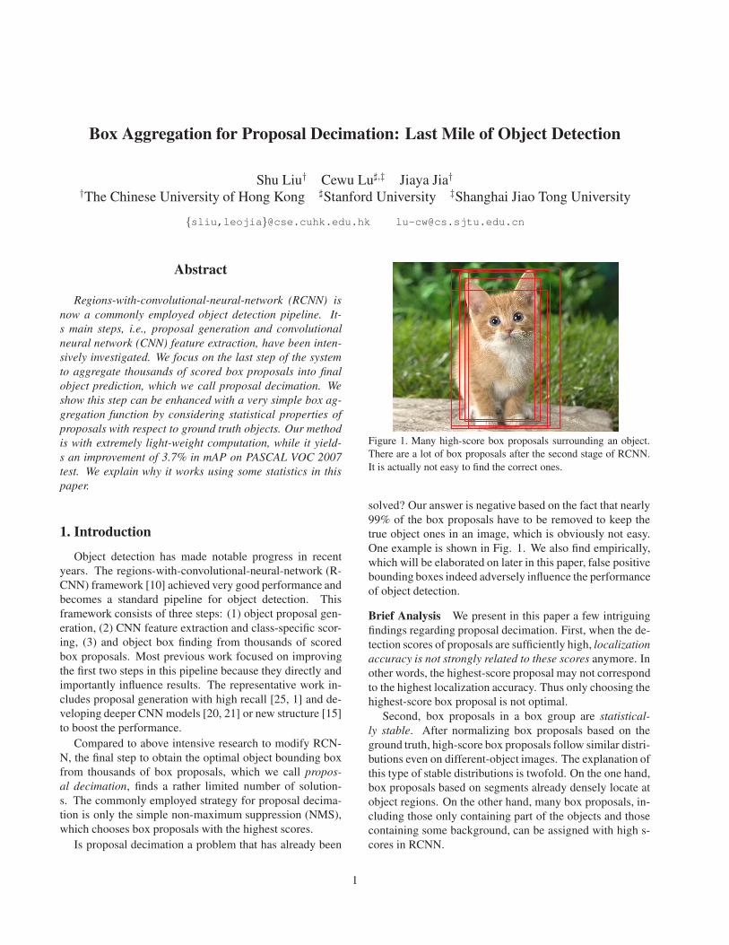
Is proposal decimation a problem that has already been

Figure 1. Many high-score box proposals surrounding an object.

There are a lot of box proposals after the second stage of RCNN.

It is actually not easy to find the correct ones.

solved? Our answer is negative based on the fact that nearly

99% of the box proposals have to be removed to keep the

true object ones in an image, which is obviously not easy.

One example is shown in Fig. 1. We also find empirically,

which will be elaborated on later in this paper, false positive

bounding boxes indeed adversely influence the performance

of object detection.

Brief Analysis We present in this paper a few intriguing

findings regarding proposal decimation. First, when the de-

tection scores of proposals are sufficiently high, localization

accuracy is not strongly related to these scores anymore. In

other words, the highest-score proposal may not correspond

to the highest localization accuracy. Thus only choosing the

highest-score box proposal is not optimal.

Second, box proposals in a box group are statistical-

ly stable. After normalizing box proposals based on the

ground truth, high-score box proposals follow similar distri-

butions even on different-object images. The explanation of

this type of stable distributions is twofold. On the one hand,

box proposals based on segments already densely locate at

object regions. On the other hand, many box proposals, in-

cluding those only containing part of the objects and those

containing some background, can be assigned with high s-

cores in RCNN.

1

Our Solution These empirical findings motivate us to

propose new schemes for proposal decimation making use

of simple but informative statistics. In this paper, a box

aggregation function is introduced with three main contri-

butions.

• We encode the statistical information of box proposals

in the function for regression.

• The number of box proposals we process varies from

image to image, which makes its modeling nontrivial.

Our function is invariant to the proposal number in dif-

ferent images, which properly addresses this difficulty.

• Solving our box aggregation function for proposal dec-

imation takes almost no computation resource and

completes immediately. This process is no more com-

plex than a few linear operations during testing and is

comparable to the naive non-maximum suppression in

terms of complexity.

Besides, we have evaluated our method on the PASCAL

VOC 2007 and 2010 detection benchmark datasets. We also

conducted ablation studies on VOC 2012 val. With the same

proposal-generation and CNN steps, detection accuracies

increase. It manifests that previous proposal-decimation

stage still has room to improve and our method shows an

promising way to accomplish it. It immediately benefits a

lot of tasks.

2. Related Work

Object detection is an important topic in computer vi-

sion and there are a large amount of methods to address the

problems in it. We review a few of them as well as recent

RCNN-related work.

Part-based Model Before RCNN is employed, part-

based models are powerful in object detection. The repre-

sentative work is deformable part-based model (DPM) [8].

It is based on HOG features and utilizes the sliding win-

dow to detect objects in an image. It can implicitly learn

appearance and location of parts by a latent structure sup-

port vector machine. Following it, in [9], DPM detector

was augmented with a segment. Part visibility reasoning

was further augmented in [2]. By adding extra context parts

[16], this model utilizes other information.

In other lines, a collection of discriminative parts were

learned [4]. One part in this collection indicates the loca-

tion of an object with a high accuracy. In [11], a detector is

represented by a single HOG template plus a dictionary of

carefully learned deformation. This kind of methods suc-

cessfully exploited representation ability of parts.

RCNN RCNN [10] is a breakthrough recently in object

detection. This method utilizes object proposal generator

[23] to obtain object proposals that may contain objects.

Then CNN features for these box proposals are extracted

and scores are assigned to the proposals by learned class-

specific classifiers. In this way, object detection is mod-

eled as classifying object proposals. By making use of C-

NN [20, 14] in representing objects, high performance is

yielded.

Several methods modified RCNN in object detection.

In [12], spatial pyramid pooling was proposed to accel-

erate feature extraction. Segmentation and context infor-

mation were used in [24] to improve the detection perfor-

mance. New training strategies and deformable layers were

designed in [17] to make CNN work better for object detec-

tion. In [21], a very deep model was proposed to enhance

the representation ability of CNN.

Since object proposals are important for final detection

performance, methods to generate object proposals with

high recall were proposed. An edge standard [25] can

distinguish boxes containing objects from background ef-

ficiently. In [1], the method followed selective search to

group high quality segments. CNN was utilized when gen-

erating object proposals [5]. In [22], object proposal gen-

erator and CNN feature extractor were combined to further

increase detection performance. These two methods show a

direction to generate locations of objects directly from neu-

ral networks.

Box Proposal Decimation We also review proposal dec-

imation methods separately since our paper focuses on it.

It refers to generating a small number of high-quality ob-

ject prediction boxes from thousands of proposals. Related

work is rather limited.

Non-maximum suppression (NMS) was widely used. It

decreases number of proposals based on an overlapping cri-

terion or other heuristics. As explained in [18], NMS in-

fluences the performance of object detection. DPM [8, 10]

used a box regression method to correct localization errors.

It does not directly take into consideration corresponding

proposals and also needs NMS to select them. The class-

specific nature makes it complex to train.

Interaction between objects was considered in [3], both

in the same class or different classes, to select box proposal-

s. The solution is a latent structure support vector machine

to search for the optimal points in the objective function.

But the result of this method could also lead to duplicate

detection.

Our method is by nature different from these strategies

since we target at high-quality prediction box generation

based on statistics of box proposals. It is similarly fast as

NMS, but generates more reliable results.

0

0.1

0.2

0.3

0.4

0.5

0.6

0.7

-1.5 -0.5 0.5 1.5 2.5 3.5

Co

rrel

atio

n

Detection Score

RCNN 8 layers

mean

max

0

0.1

0.2

0.3

0.4

0.5

0.6

0.7

0.8

0.9

-1.5 -0.5 0.5 1.5 2.5 3.5

Corr

elat

ion

Detection Score

RCNN 16 layers

mean

max

(a) (b)

0

0.1

0.2

0.3

0.4

0.5

0.6

0.7

0.8

-1 0 1 2 3 4

Co

rrel

atio

n

Detection Score

RCNN 8 layers

mean

max

0

0.1

0.2

0.3

0.4

0.5

0.6

0.7

0.8

0.9

-1 0 1 2 3 4

Co

rrel

atio

n

Detection Score

RCNN 16 layers

mean

max

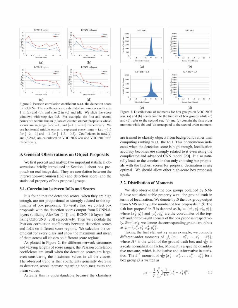
(c) (d)Figure 2. Pearson correlation coefficient w.r.t. the detection score

for RCNNs. The coefficients are calculated on windows with size

1 in (a) and (b), and size 2 in (c) and (d). We slide the score

windows with step-size 0.5. For example, the first and second

points of the blue line in (a) are calculated on box proposals whose

scores are in range [−2,−1] and [−1.5,−0.5] respectively. We

use horizontal middle scores to represent every range – i.e., −1.5for [−2,−1] and −1 for [−1.5,−0.5]. Coefficients in (a)&(c)

and (b)&(d) are calculated on VOC 2007 test and VOC 2010 val,

respectively.

3. General Observations on Object Proposals

We first present and analyze two important statistical ob-

servations briefly introduced in Section 1 about box pro-

posals on real image data. They are correlation between the

intersection-over-union (IoU) and detection score, and the

statistical property of box proposal groups.

3.1. Correlation between IoUs and Scores

It is found that the detection scores, when they are high

enough, are not proportional or strongly related to the op-

timality of box proposals. To verify this, we collect box

proposals with the detection scores output from RCNN-8-

layers (utilizing AlexNet [14]) and RCNN-16-layers (uti-

lizing OxfordNet [20]) respectively. Then we calculate the

Pearson correlation coefficients between detection scores

and IoUs on different score regions. We calculate the co-

efficient for every class and show the maximum and mean

of them across all classes on different score regions.

As plotted in Figure 2, for different network structures

and varying lengths of score ranges, the Pearson correlation

coefficients are small when the detection scores are large,

even considering the maximum values in all the classes.

The observed trend is that coefficients generally decrease

as detection scores increase regarding both maximum and

mean values.

Actually this is understandable because the classifiers

0

500

1000

1500

2000

2500

3000

-2 -1.5 -1 -0.5 0 0.5 1

Num

ber

of

Box

Gro

ups

First Order Moment

IoU > 0.5

0

1000

2000

3000

4000

5000

6000

7000

8000

9000

0 0.5 1 1.5 2 2.5 3

Num

ber

of

Box

Gro

ups

Second Order Moment

IoU > 0.5

(a) (b)

0

500

1000

1500

2000

2500

-2 -1.5 -1 -0.5 0 0.5 1

Num

ber

of

Box

Gro

ups

First Order Moment

0.2 < IoU < 0.5

0

1000

2000

3000

4000

5000

6000

7000

8000

9000

0 0.5 1 1.5 2 2.5 3

Nu

mb

er o

f B

ox

Gro

up

s

Second Order Moment

0.2 < IoU < 0.5

(c) (d)Figure 3. Distributions of moments for box groups on VOC 2007

test. (a) and (b) correspond to the first set of box groups while (c)

and (d) refer to the second set. (a) and (c) contain the first order

moment while (b) and (d) correspond to the second order moment.

are trained to classify objects from background rather than

computing ranking w.r.t. the IoU. This phenomenon indi-

cates when the detection score is high enough, localization

accuracy becomes not strongly related to it even using the

complicated and advanced CNN model [20]. It also natu-

rally leads to the conclusion that only choosing box propos-

als with the highest scores for proposal decimation is not

optimal. We should allow other high-score box proposals

speak.

3.2. Distribution of Moments

We also observe that the box groups obtained by NM-

S have statistical stable property w.r.t. the ground truth in

terms of localization. We denote by B the box group output

from NMS and by p the number of box proposals in B. The

i-th box proposal in B is denoted as bi = {xi1, y

i1, x

i2, y

i2},

where (xi1, yi

1) and (xi

2, yi

2) are the coordinates of the top-

left and bottom-right corners of the box proposal respective-

ly. Similarly, we denote the corresponding ground truth box

as g = {xg1, y

g1, x

g2, y

g2}.

Taking the first element x1 as an example, we compute

different-order moments of 1

Hg {x11 − x

g1, . . . , x

p1− x

g1},

where Hg is the width of the ground truth box and 1

Hg is

a scale normalization factor. Moment is a specific quantita-

tive measure, which is indicative and informative in statis-

tics. The kth moment of 1

Hg {x1

1− x

g1, . . . , x

p1− x

g1} for a

box group B is written as

µk =1

p

p∑

i=1

[1

Hg(xi

1− x

g1)]k. (1)

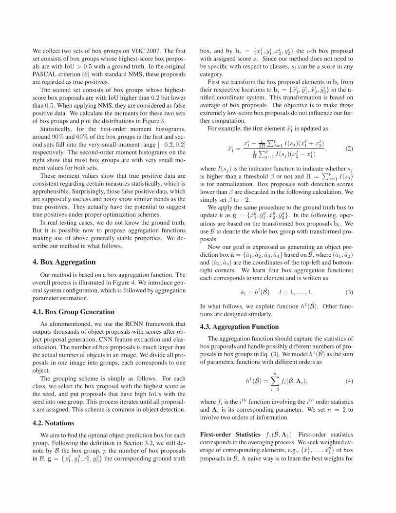
We collect two sets of box groups on VOC 2007. The first

set consists of box groups whose highest-score box propos-

als are with IoU > 0.5 with a ground truth. In the original

PASCAL criterion [6] with standard NMS, these proposals

are regarded as true positives.

The second set consists of box groups whose highest-

score box proposals are with IoU higher than 0.2 but lower

than 0.5. When applying NMS, they are considered as false

positive data. We calculate the moments for these two sets

of box groups and plot the distributions in Figure 3.

Statistically, for the first-order moment histograms,

around 90% and 60% of the box groups in the first and sec-

ond sets fall into the very-small-moment range [−0.2, 0.2]respectively. The second-order moment histograms on the

right show that most box groups are with very small mo-

ment values for both sets.

These moment values show that true positive data are

consistent regarding certain measures statistically, which is

apprehensible. Surprisingly, those false positive data, which

are supposedly useless and noisy show similar trends as the

true positives. They actually have the potential to suggest

true positives under proper optimization schemes.

In real testing cases, we do not know the ground truth.

But it is possible now to propose aggregation functions

making use of above generally stable properties. We de-

scribe our method in what follows.

4. Box Aggregation

Our method is based on a box aggregation function. The

overall process is illustrated in Figure 4. We introduce gen-

eral system configuration, which is followed by aggregation

parameter estimation.

4.1. Box Group Generation

As aforementioned, we use the RCNN framework that

outputs thousands of object proposals with scores after ob-

ject proposal generation, CNN feature extraction and clas-

sification. The number of box proposals is much larger than

the actual number of objects in an image. We divide all pro-

posals in one image into groups, each corresponds to one

object.

The grouping scheme is simply as follows. For each

class, we select the box proposal with the highest score as

the seed, and put proposals that have high IoUs with the

seed into one group. This process iterates until all proposal-

s are assigned. This scheme is common in object detection.

4.2. Notations

We aim to find the optimal object prediction box for each

group. Following the definition in Section 3.2, we still de-

note by B the box group, p the number of box proposals

in B, g = {xg1, y

g1, x

g2, y

g2} the corresponding ground truth

box, and by bi = {xi1, yi

1, xi

2, yi

2} the i-th box proposal

with assigned score si. Since our method does not need to

be specific with respect to classes, si can be a score in any

category.

First we transform the box proposal elements in bi from

their respective locations to bi = {xi1, yi

1, xi

2, yi

2} in the u-

nified coordinate system. This transformation is based on

average of box proposals. The objective is to make those

extremely low-score box proposals do not influence our fur-

ther computation.

For example, the first element xi1

is updated as

xi1=

xi1 −

1

2Π

∑p

j=1I(sj)(x

j1+ x

j2)

1

Π

∑p

j=1I(sj)(x

j2− x

j1)

, (2)

where I(sj) is the indicator function to indicate whether sjis higher than a threshold β or not and Π =

∑p

j=1I(sj)

is for normalization. Box proposals with detection scores

lower than β are discarded in the following calculation. We

simply set β to −2.

We apply the same procedure to the ground truth box to

update it as g = {xg1, y

g1, x

g2, y

g2}. In the following, oper-

ations are based on the transformed box proposals bi. We

use B to denote the whole box group with transformed pro-

posals.

Now our goal is expressed as generating an object pre-

diction box a = {a1, a2, a3, a4} based on B, where (a1, a2)and (a3, a4) are the coordinates of the top-left and bottom-

right corners. We learn four box aggregation functions;

each corresponds to one element and is written as

al = hl(B) l = 1, . . . , 4. (3)

In what follows, we explain function h1(B). Other func-

tions are designed similarly.

4.3. Aggregation Function

The aggregation function should capture the statistics of

box proposals and handle possibly different numbers of pro-

posals in box groups in Eq. (3). We model h1(B) as the sum

of parametric functions with different orders as

h1(B) =

n∑

i=0

fi(B,Λi), (4)

where fi is the ith function involving the ith order statistics

and Λi is its corresponding parameter. We set n = 2 to

involve two orders of information.

First-order Statistics f1(B,Λ1) First-order statistics

corresponds to the averaging process. We seek weighted av-

erage of corresponding elements, e.g., {x1

1, . . . , x

p1} of box

proposals in B. A naive way is to learn the best weights for

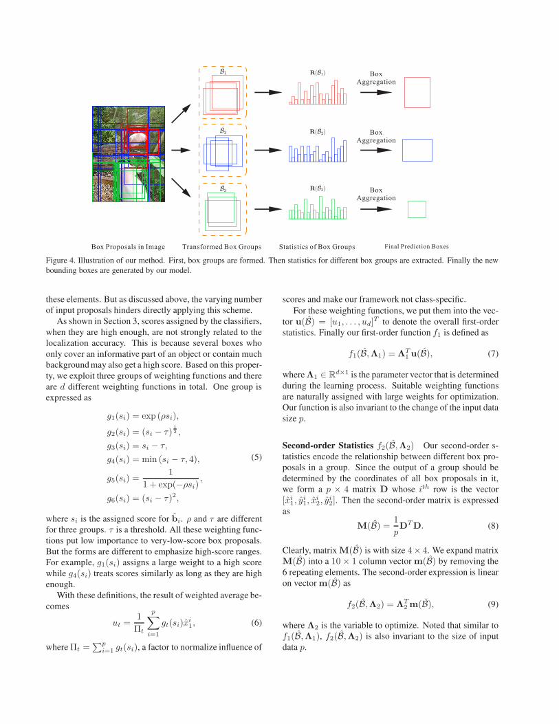
Box Proposals in Image Transformed Box Groups Statistics of Box Groups Final Prediction Boxes

BoxAggregation

BoxAggregation

BoxAggregation

Figure 4. Illustration of our method. First, box groups are formed. Then statistics for different box groups are extracted. Finally the new

bounding boxes are generated by our model.

these elements. But as discussed above, the varying number

of input proposals hinders directly applying this scheme.

As shown in Section 3, scores assigned by the classifiers,

when they are high enough, are not strongly related to the

localization accuracy. This is because several boxes who

only cover an informative part of an object or contain much

background may also get a high score. Based on this proper-

ty, we exploit three groups of weighting functions and there

are d different weighting functions in total. One group is

expressed as

g1(si) = exp (ρsi),

g2(si) = (si − τ)1

2 ,

g3(si) = si − τ,

g4(si) = min (si − τ, 4),

g5(si) =1

1 + exp(−ρsi),

g6(si) = (si − τ)2,

(5)

where si is the assigned score for bi. ρ and τ are different

for three groups. τ is a threshold. All these weighting func-

tions put low importance to very-low-score box proposals.

But the forms are different to emphasize high-score ranges.

For example, g1(si) assigns a large weight to a high score

while g4(si) treats scores similarly as long as they are high

enough.

With these definitions, the result of weighted average be-

comes

ut =1

Πt

p∑

i=1

gt(si)xi1, (6)

where Πt =∑p

i=1gt(si), a factor to normalize influence of

scores and make our framework not class-specific.

For these weighting functions, we put them into the vec-

tor u(B) = [u1, . . . , ud]T to denote the overall first-order

statistics. Finally our first-order function f1 is defined as

f1(B,Λ1) = ΛT1u(B), (7)

whereΛ1 ∈ Rd×1 is the parameter vector that is determined

during the learning process. Suitable weighting functions

are naturally assigned with large weights for optimization.

Our function is also invariant to the change of the input data

size p.

Second-order Statistics f2(B,Λ2) Our second-order s-

tatistics encode the relationship between different box pro-

posals in a group. Since the output of a group should be

determined by the coordinates of all box proposals in it,

we form a p × 4 matrix D whose ith row is the vector

[xi1, yi

1, xi

2, yi

2]. Then the second-order matrix is expressed

as

M(B) =1

pDTD. (8)

Clearly, matrix M(B) is with size 4× 4. We expand matrix

M(B) into a 10 × 1 column vector m(B) by removing the

6 repeating elements. The second-order expression is linear

on vector m(B) as

f2(B,Λ2) = ΛT2 m(B), (9)

where Λ2 is the variable to optimize. Noted that similar to

f1(B,Λ1), f2(B,Λ2) is also invariant to the size of input

data p.

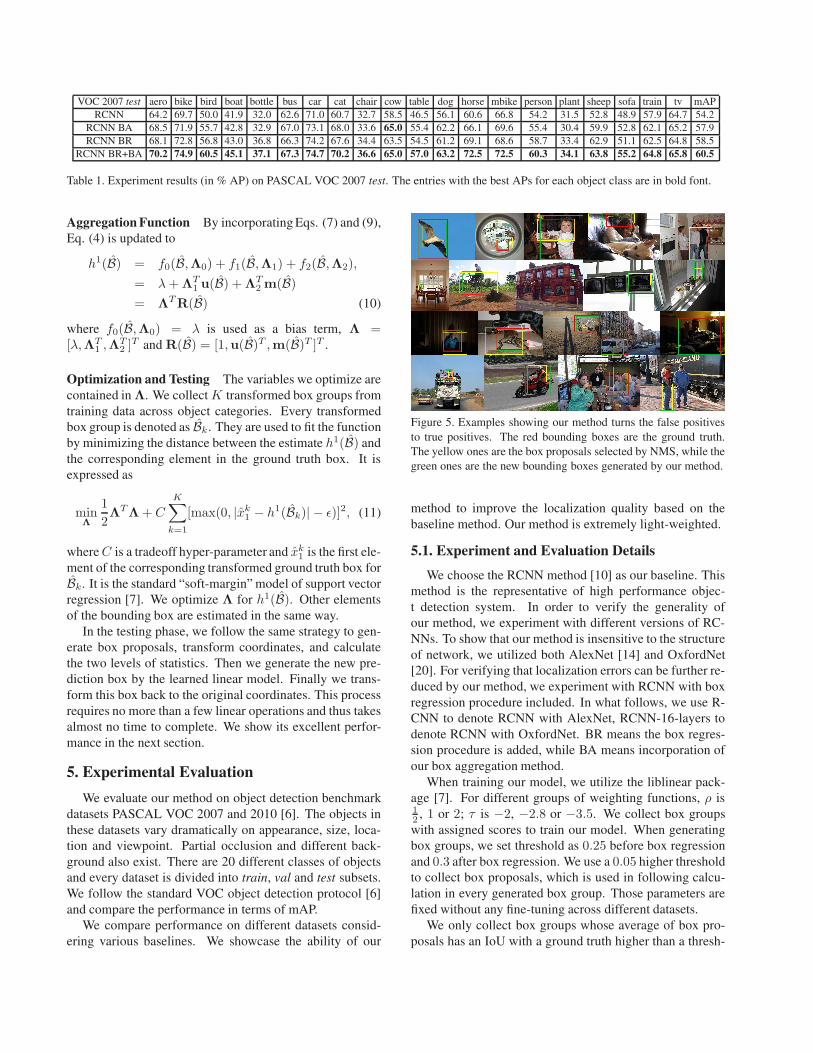
VOC 2007 test aero bike bird boat bottle bus car cat chair cow table dog horse mbike person plant sheep sofa train tv mAP

RCNN 64.2 69.7 50.0 41.9 32.0 62.6 71.0 60.7 32.7 58.5 46.5 56.1 60.6 66.8 54.2 31.5 52.8 48.9 57.9 64.7 54.2

RCNN BA 68.5 71.9 55.7 42.8 32.9 67.0 73.1 68.0 33.6 65.0 55.4 62.2 66.1 69.6 55.4 30.4 59.9 52.8 62.1 65.2 57.9

RCNN BR 68.1 72.8 56.8 43.0 36.8 66.3 74.2 67.6 34.4 63.5 54.5 61.2 69.1 68.6 58.7 33.4 62.9 51.1 62.5 64.8 58.5

RCNN BR+BA 70.2 74.9 60.5 45.1 37.1 67.3 74.7 70.2 36.6 65.0 57.0 63.2 72.5 72.5 60.3 34.1 63.8 55.2 64.8 65.8 60.5

Table 1. Experiment results (in % AP) on PASCAL VOC 2007 test. The entries with the best APs for each object class are in bold font.

Aggregation Function By incorporating Eqs. (7) and (9),

Eq. (4) is updated to

h1(B) = f0(B,Λ0) + f1(B,Λ1) + f2(B,Λ2),

= λ+ΛT1 u(B) +ΛT

2 m(B)

= ΛTR(B) (10)

where f0(B,Λ0) = λ is used as a bias term, Λ =[λ,ΛT

1 ,ΛT2 ]

T and R(B) = [1,u(B)T ,m(B)T ]T .

Optimization and Testing The variables we optimize are

contained in Λ. We collect K transformed box groups from

training data across object categories. Every transformed

box group is denoted as Bk. They are used to fit the function

by minimizing the distance between the estimate h1(B) and

the corresponding element in the ground truth box. It is

expressed as

minΛ

1

2ΛTΛ+ C

K∑

k=1

[max(0, |xk1− h1(Bk)| − ǫ)]2, (11)

whereC is a tradeoff hyper-parameter and xk1

is the first ele-

ment of the corresponding transformed ground truth box for

Bk. It is the standard “soft-margin” model of support vector

regression [7]. We optimize Λ for h1(B). Other elements

of the bounding box are estimated in the same way.

In the testing phase, we follow the same strategy to gen-

erate box proposals, transform coordinates, and calculate

the two levels of statistics. Then we generate the new pre-

diction box by the learned linear model. Finally we trans-

form this box back to the original coordinates. This process

requires no more than a few linear operations and thus takes

almost no time to complete. We show its excellent perfor-

mance in the next section.

5. Experimental Evaluation

We evaluate our method on object detection benchmark

datasets PASCAL VOC 2007 and 2010 [6]. The objects in

these datasets vary dramatically on appearance, size, loca-

tion and viewpoint. Partial occlusion and different back-

ground also exist. There are 20 different classes of objects

and every dataset is divided into train, val and test subsets.

We follow the standard VOC object detection protocol [6]

and compare the performance in terms of mAP.

We compare performance on different datasets consid-

ering various baselines. We showcase the ability of our

Figure 5. Examples showing our method turns the false positives

to true positives. The red bounding boxes are the ground truth.

The yellow ones are the box proposals selected by NMS, while the

green ones are the new bounding boxes generated by our method.

method to improve the localization quality based on the

baseline method. Our method is extremely light-weighted.

5.1. Experiment and Evaluation Details

We choose the RCNN method [10] as our baseline. This

method is the representative of high performance objec-

t detection system. In order to verify the generality of

our method, we experiment with different versions of RC-

NNs. To show that our method is insensitive to the structure

of network, we utilized both AlexNet [14] and OxfordNet

[20]. For verifying that localization errors can be further re-

duced by our method, we experiment with RCNN with box

regression procedure included. In what follows, we use R-

CNN to denote RCNN with AlexNet, RCNN-16-layers to

denote RCNN with OxfordNet. BR means the box regres-

sion procedure is added, while BA means incorporation of

our box aggregation method.

When training our model, we utilize the liblinear pack-

age [7]. For different groups of weighting functions, ρ is1

2, 1 or 2; τ is −2, −2.8 or −3.5. We collect box groups

with assigned scores to train our model. When generating

box groups, we set threshold as 0.25 before box regression

and 0.3 after box regression. We use a 0.05 higher threshold

to collect box proposals, which is used in following calcu-

lation in every generated box group. Those parameters are

fixed without any fine-tuning across different datasets.

We only collect box groups whose average of box pro-

posals has an IoU with a ground truth higher than a thresh-

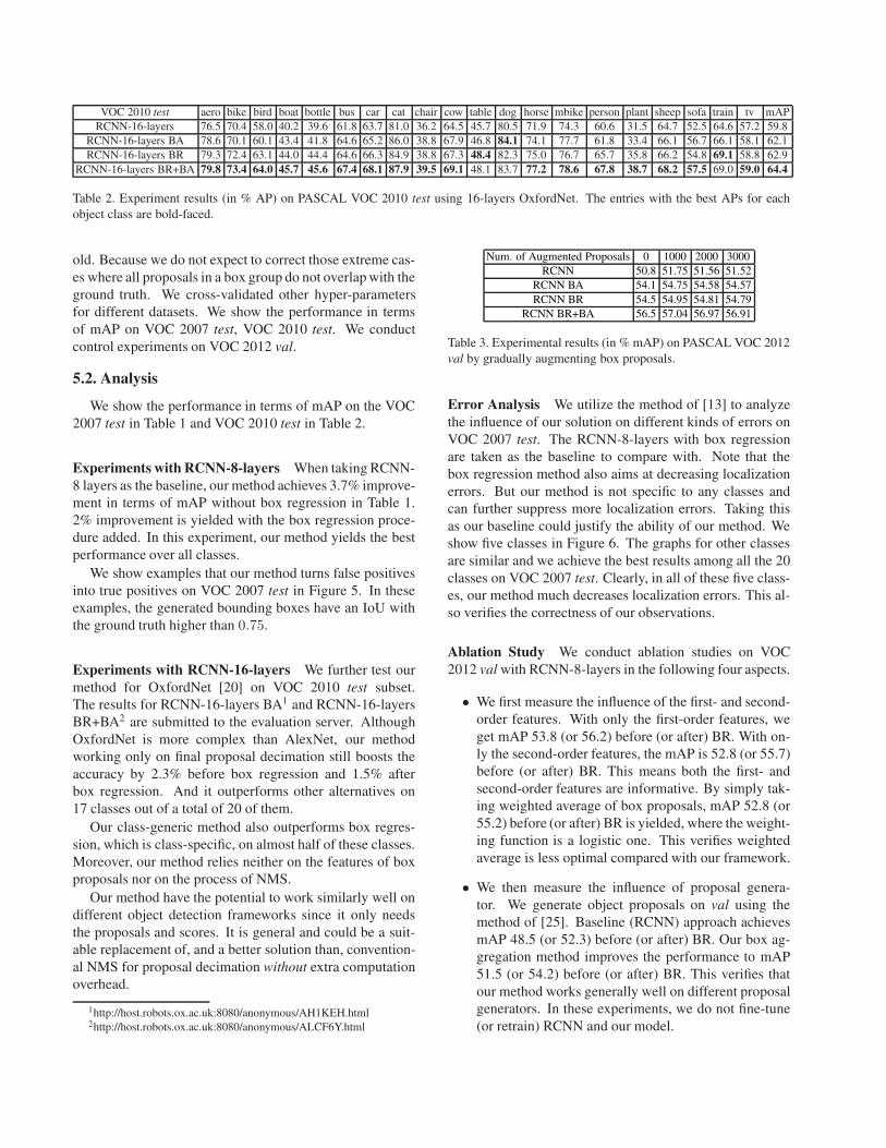
VOC 2010 test aero bike bird boat bottle bus car cat chair cow table dog horse mbike person plant sheep sofa train tv mAP

RCNN-16-layers 76.5 70.4 58.0 40.2 39.6 61.8 63.7 81.0 36.2 64.5 45.7 80.5 71.9 74.3 60.6 31.5 64.7 52.5 64.6 57.2 59.8

RCNN-16-layers BA 78.6 70.1 60.1 43.4 41.8 64.6 65.2 86.0 38.8 67.9 46.8 84.1 74.1 77.7 61.8 33.4 66.1 56.7 66.1 58.1 62.1

RCNN-16-layers BR 79.3 72.4 63.1 44.0 44.4 64.6 66.3 84.9 38.8 67.3 48.4 82.3 75.0 76.7 65.7 35.8 66.2 54.8 69.1 58.8 62.9

RCNN-16-layers BR+BA 79.8 73.4 64.0 45.7 45.6 67.4 68.1 87.9 39.5 69.1 48.1 83.7 77.2 78.6 67.8 38.7 68.2 57.5 69.0 59.0 64.4

Table 2. Experiment results (in % AP) on PASCAL VOC 2010 test using 16-layers OxfordNet. The entries with the best APs for each

object class are bold-faced.

old. Because we do not expect to correct those extreme cas-

es where all proposals in a box group do not overlap with the

ground truth. We cross-validated other hyper-parameters

for different datasets. We show the performance in terms

of mAP on VOC 2007 test, VOC 2010 test. We conduct

control experiments on VOC 2012 val.

5.2. Analysis

We show the performance in terms of mAP on the VOC

2007 test in Table 1 and VOC 2010 test in Table 2.

Experiments with RCNN-8-layers When taking RCNN-

8 layers as the baseline, our method achieves 3.7% improve-

ment in terms of mAP without box regression in Table 1.

2% improvement is yielded with the box regression proce-

dure added. In this experiment, our method yields the best

performance over all classes.

We show examples that our method turns false positives

into true positives on VOC 2007 test in Figure 5. In these

examples, the generated bounding boxes have an IoU with

the ground truth higher than 0.75.

Experiments with RCNN-16-layers We further test our

method for OxfordNet [20] on VOC 2010 test subset.

The results for RCNN-16-layers BA1 and RCNN-16-layers

BR+BA2 are submitted to the evaluation server. Although

OxfordNet is more complex than AlexNet, our method

working only on final proposal decimation still boosts the

accuracy by 2.3% before box regression and 1.5% after

box regression. And it outperforms other alternatives on

17 classes out of a total of 20 of them.

Our class-generic method also outperforms box regres-

sion, which is class-specific, on almost half of these classes.

Moreover, our method relies neither on the features of box

proposals nor on the process of NMS.

Our method have the potential to work similarly well on

different object detection frameworks since it only needs

the proposals and scores. It is general and could be a suit-

able replacement of, and a better solution than, convention-

al NMS for proposal decimation without extra computation

overhead.

1http://host.robots.ox.ac.uk:8080/anonymous/AH1KEH.html2http://host.robots.ox.ac.uk:8080/anonymous/ALCF6Y.html

Num. of Augmented Proposals 0 1000 2000 3000

RCNN 50.8 51.75 51.56 51.52

RCNN BA 54.1 54.75 54.58 54.57

RCNN BR 54.5 54.95 54.81 54.79

RCNN BR+BA 56.5 57.04 56.97 56.91

Table 3. Experimental results (in % mAP) on PASCAL VOC 2012

val by gradually augmenting box proposals.

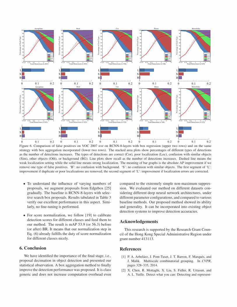
Error Analysis We utilize the method of [13] to analyze

the influence of our solution on different kinds of errors on

VOC 2007 test. The RCNN-8-layers with box regression

are taken as the baseline to compare with. Note that the

box regression method also aims at decreasing localization

errors. But our method is not specific to any classes and

can further suppress more localization errors. Taking this

as our baseline could justify the ability of our method. We

show five classes in Figure 6. The graphs for other classes

are similar and we achieve the best results among all the 20

classes on VOC 2007 test. Clearly, in all of these five class-

es, our method much decreases localization errors. This al-

so verifies the correctness of our observations.

Ablation Study We conduct ablation studies on VOC

2012 val with RCNN-8-layers in the following four aspects.

• We first measure the influence of the first- and second-

order features. With only the first-order features, we

get mAP 53.8 (or 56.2) before (or after) BR. With on-

ly the second-order features, the mAP is 52.8 (or 55.7)

before (or after) BR. This means both the first- and

second-order features are informative. By simply tak-

ing weighted average of box proposals, mAP 52.8 (or

55.2) before (or after) BR is yielded, where the weight-

ing function is a logistic one. This verifies weighted

average is less optimal compared with our framework.

• We then measure the influence of proposal genera-

tor. We generate object proposals on val using the

method of [25]. Baseline (RCNN) approach achieves

mAP 48.5 (or 52.3) before (or after) BR. Our box ag-

gregation method improves the performance to mAP

51.5 (or 54.2) before (or after) BR. This verifies that

our method works generally well on different proposal

generators. In these experiments, we do not fine-tune

(or retrain) RCNN and our model.

T Dotal etections (x 285)

PE

Terc

en

tag

e o

fach

yp

e

Aeroplane

0.125 0. 25 0. 5 1 2 4 80

10

20

30

40

50

60

70

80

90

100

Cor

Loc

Sim

Oth

BG

T Dotal etections (x 459)

PE

Terc

en

tag

e o

fach

yp

e

Bird

0.125 0.25 0.5 1 2 4 80

10

20

30

40

50

60

70

80

90

100

Cor

Loc

Sim

Oth

BG

T Dotal etections (x 358)

PE

Terc

en

tag

e o

fach

yp

e

Cat

0.125 0.25 0.5 1 2 4 80

10

20

30

40

50

60

70

80

90

100

Cor

Loc

Sim

Oth

BG

T Dotal etections (x 348)

PE

Terc

en

tag

e o

fach

yp

e

Horse

0.125 0.25 0.5 1 2 4 80

10

20

30

40

50

60

70

80

90

100

Cor

Loc

Sim

Oth

BG

T Dotal etections (x 325)

PE

Terc

en

tag

e o

fach

yp

e

Motorbike

0.125 0.25 0.5 1 2 4 80

10

20

30

40

50

60

70

80

90

100

Cor

Loc

Sim

Oth

BG

0 0.1 0.2

B

S

L

0 0.1 0.2

B

S

L

0 0.1 0.2

B

S

L

0 0.1 0.2

B

S

L

0 0.1 0.2

B

S

L

T Dotal etections (x 285)

PE

Terc

en

tag

e o

fach

yp

e

Aeroplane

0.125 0.25 0.5 1 2 4 80

10

20

30

40

50

60

70

80

90

100

Cor

Loc

Sim

Oth

BG

T Dotal etections (x 459)

PE

Terc

en

tag

e o

fach

yp

e

Bird

0.125 0.25 0.5 1 2 4 80

10

20

30

40

50

60

70

80

90

100

Cor

Loc

Sim

Oth

BG

T Dotal etections (x 358)

PE

Terc

en

tag

e o

fach

yp

e

Cat

0.125 0.25 0.5 1 2 4 80

10

20

30

40

50

60

70

80

90

100

Cor

Loc

Sim

Oth

BG

T Dotal etections (x 348)

PE

Ter

cen

tag

e o

fac

hy

pe

Horse

0.125 0.25 0.5 1 2 4 80

10

20

30

40

50

60

70

80

90

100

Cor

Loc

Sim

Oth

BG

T Dotal etections (x 325)

PE

Terc

en

tag

e o

fach

yp

e

Motorbike

0.125 0.25 0.5 1 2 4 80

10

20

30

40

50

60

70

80

90

100

Cor

Loc

Sim

Oth

BG

0 0.1 0.2

B

S

L

0 0.1 0.2

B

S

L

0 0.1 0.2

B

S

L

0 0.1 0.2

B

S

L

0 0.1 0.2

B

S

L

Figure 6. Comparison of false positives on VOC 2007 test on RCNN-8-layers with box regression (upper two rows) and on the same

strategy with box aggregation incorporated (lower two rows). The stacked area plots show percentages of different types of detections

as the number of detections increases. The types of detections are correct (Cor), poor localization (Loc), confusion with similar objects

(Sim), other objects (Oth), or background (BG). Line plots show recall as the number of detections increases. Dashed line means the

weak localization setting while the solid line means strong localization. The meaning of bar graphs is the absolute AP improvement if we

remove one type of false positives. ‘B’: no confusion with background. ‘S’: no confusion with similar objects. The first segment of ‘L’:

improvement if duplicate or poor localizations are removed; the second segment of ‘L’: improvement if localization errors are corrected.

• To understand the influence of varying numbers of

proposals, we augment proposals from Edgebox [25]

gradually. The baseline is RCNN-8-layers with selec-

tive search box proposals. Results tabulated in Table 3

verify our excellent performance in this aspect. Simi-

larly, no fine-tuning is performed.

• For score normalization, we follow [19] to calibrate

detection scores for different classes and feed them to

our method. The result is mAP 53.9 (or 56.3) before

(or after) BR. It means that our normalization step in

Eq. (6) already fulfills the duty of score normalization

for different classes nicely.

6. Conclusion

We have identified the importance of the final stage, i.e.,

proposal decimation in object detection and presented our

statistical observation. A box aggregation method to finally

improve the detection performance was proposed. It is class

generic and does not increase computation overhead even

compared to the extremely simple non-maximum suppres-

sion. We evaluated our method on different datasets con-

sidering different deep neural network architectures, under

different parameter configurations, and compared to various

baseline methods. Our proposed method showed its ability

and generality. It can be incorporated into existing object

detection systems to improve detection accuracies.

Acknowledgements

This research is supported by the Research Grant Coun-

cil of the Hong Kong Special Administrative Region under

grant number 413113.

References

[1] P. A. Arbelaez, J. Pont-Tuset, J. T. Barron, F. Marques, and

J. Malik. Multiscale combinatorial grouping. In CVPR,

pages 328–335, 2014.

[2] X. Chen, R. Mottaghi, X. Liu, S. Fidler, R. Urtasun, and

A. L. Yuille. Detect what you can: Detecting and represent-

ing objects using holistic models and body parts. In ICCV,

pages 1979–1986, 2014.

[3] C. Desai, D. Ramanan, and C. C. Fowlkes. Discrimina-

tive models for multi-class object layout. IJCV, 95(1):1–12,

2011.

[4] I. Endres, K. J. Shih, J. Jiaa, and D. Hoiem. Learning collec-

tions of part models for object recognition. In CVPR, pages

939–946, 2013.

[5] D. Erhan, C. Szegedy, A. Toshev, and D. Anguelov. Scalable

object detection using deep neural networks. In CVPR, pages

2155–2162, 2014.

[6] M. Everingham, S. M. A. Eslami, L. V. Gool, C. K. I.

Williams, J. M. Winn, and A. Zisserman. The pascal visual

object classes challenge: A retrospective. IJCV, 111(1):98–

136, 2015.

[7] R. Fan, K. Chang, C. Hsieh, X. Wang, and C. Lin. LIB-

LINEAR: A library for large linear classification. JMLR,

9:1871–1874, 2008.

[8] P. F. Felzenszwalb, D. A. McAllester, and D. Ramanan. A

discriminatively trained, multiscale, deformable part model.

In CVPR, 2008.

[9] S. Fidler, R. Mottaghi, A. L. Yuille, and R. Urtasun. Bottom-

up segmentation for top-down detection. In CVPR, pages

3294–3301, 2013.

[10] R. B. Girshick, J. Donahue, T. Darrell, and J. Malik. Rich

feature hierarchies for accurate object detection and semantic

segmentation. In CVPR, pages 580–587, 2014.

[11] B. Hariharan, C. L. Zitnick, and P. Dollar. Detecting objects

using deformation dictionaries. In CVPR, pages 1995–2002,

2014.

[12] K. He, X. Zhang, S. Ren, and J. Sun. Spatial pyramid pool-

ing in deep convolutional networks for visual recognition.

CoRR, abs/1406.4729, 2014.

[13] D. Hoiem, Y. Chodpathumwan, and Q. Dai. Diagnosing error

in object detectors. In ECCV, pages 340–353, 2012.

[14] A. Krizhevsky, I. Sutskever, and G. E. Hinton. Imagenet

classification with deep convolutional neural networks. In

NIPS, pages 1106–1114, 2012.

[15] M. Lin, Q. Chen, and S. Yan. Network in network. CoRR,

abs/1312.4400, 2013.

[16] R. Mottaghi, X. Chen, X. Liu, N. Cho, S. Lee, S. Fidler,

R. Urtasun, and A. L. Yuille. The role of context for object

detection and semantic segmentation in the wild. In CVPR,

pages 891–898, 2014.

[17] W. Ouyang, P. Luo, X. Zeng, S. Qiu, Y. Tian, H. Li, S. Yang,

Z. Wang, Y. Xiong, C. Qian, Z. Zhu, R. Wang, C. C. Loy,

X. Wang, and X. Tang. Deepid-net: multi-stage and de-

formable deep convolutional neural networks for object de-

tection. CoRR, abs/1409.3505, 2014.

[18] D. Parikh and C. Zitnick. Human-debugging of machines.

NIPS WCSSWC, 2:7, 2011.

[19] J. C. Platt. Probabilistic outputs for support vector machines

and comparisons to regularized likelihood methods. In AD-

VANCES IN LARGE MARGIN CLASSIFIERS, pages 61–74,

1999.

[20] K. Simonyan and A. Zisserman. Very deep convolution-

al networks for large-scale image recognition. CoRR, ab-

s/1409.1556, 2014.

[21] C. Szegedy, W. Liu, Y. Jia, P. Sermanet, S. Reed,

D. Anguelov, D. Erhan, V. Vanhoucke, and A. Rabinovich.

Going deeper with convolutions. CoRR, abs/1409.4842,

2014.

[22] C. Szegedy, S. Reed, D. Erhan, and D. Anguelov. Scalable,

high-quality object detection. CoRR, abs/1412.1441, 2014.

[23] K. E. A. van de Sande, J. R. R. Uijlings, T. Gevers, and

A. W. M. Smeulders. Segmentation as selective search for

object recognition. In ICCV, pages 1879–1886, 2011.

[24] Y. Zhu, R. Urtasun, R. Salakhutdinov, and S. Fidler.

segDeepM: Exploiting Segmentation and Context in Deep

Neural Networks for Object Detection. In CVPR, 2015.

[25] C. L. Zitnick and P. Dollar. Edge boxes: Locating object

proposals from edges. In ECCV, pages 391–405, 2014.