Meccanica (2014) 49:441–467DOI 10.1007/s11012-013-9804-x

Boundary-layer receptivity to external disturbances usingmultiple scales

Simone Zuccher · Paolo Luchini

Received: 17 October 2012 / Accepted: 27 August 2013 / Published online: 14 September 2013© Springer Science+Business Media Dordrecht 2013

Abstract Non-homogeneous multiple scales are in-troduced to solve the resonant problem of non-parallelboundary-layer receptivity originating from thequadratic mixing of environmental disturbances. Theresulting algorithm is computationally inexpensiveand can be efficiently included in industrial codes fortransition prediction. The mutual interactions betweenacoustic wave, vorticity wave, wall vibration and wallroughness are discussed in detail and the receptivitycoefficient, which relates the amplitude of the excitedwave to the amplitude of the exciting sources, is com-puted. The largest effect is found for the interactionbetween acoustic waves and wall roughness pertur-bations. Other coupling mechanisms are less effec-tive. By comparing parallel and non-parallel results,it is found that flow non-parallelism can play a non-negligible role even in Blasius’ boundary layer, al-though the largest effects are evident for the three-dimensional boundary layer over an infinite sweptwing. For the particular case of wall roughness—wallvibration mixing, the velocity disturbance is shown tobe exactly equal to the velocity perturbation induced

S. Zuccher (B)Department of Computer Science, Università di Verona,37134 Verona, Italye-mail: simone.zuccher@univr.it

P. LuchiniDepartment of Industrial Engineering,Università di Salerno, 84084 Fisciano, SA, Italye-mail: luchini@unisa.it

by wall roughness alone on a wall vibrating in the nor-mal direction.

Keywords Boundary-layer receptivity ·Boundary-layer stability · Flow instabilities ·Transition to turbulence · Multiple scales ·Receptivity to external disturbances

1 Introduction to the problem of receptivity

Within the scope of boundary-layer stability analysis,receptivity [49, 52] has been receiving large attentionin the last decades owing to its potential to improvetransition-prediction criteria by including the responseto external disturbances. The classical eN method, stillemployed for airplane design, is based on the ansatzthat transition occurs when the total amplification ofthe leading instability mode (obtained as the solutionto a homogeneous problem) attains a given value. Thisis only a realistic assumption for practical situationswhere both the transition threshold and the amplitudeof external sources of excitation exhibit little varia-tion from one case to another. Here, instead, we fo-cus on the relationship between the amplitude of theTollmien-Schlichting instability wave (TS wave) gen-erated inside the boundary layer and the physical am-plitude of the environmental disturbances that cause it.

Typical external disturbances are acoustic waves,freestream vorticity waves and wall vibrations. Evenwhen their frequency is close to that of TS waves,

442 Meccanica (2014) 49:441–467

these disturbances cannot resonate with TS waves be-cause their wavelength is much larger.1 On the otherhand, resonance can be achieved if some wavelengthconversion mechanism ensures the adaptation of theexciting wavelength [30, 31, 53]. This wavelength-conversion effect can be provided by the rapid growthof the boundary layer near the leading edge or by arapid variation of the wall boundary conditions thatinduce a fast adaptation of the boundary layer. Con-sequently, the wide range of receptivity configura-tions analyzed in published works (see Ref. [33] fora review on the progresses made in the 1980s andRef. [57] for a later review summarizing theoreticalmodeling, numerical simulations, and experiments)can ultimately be grouped as (a) leading-edge recep-tivity, (b) sudden boundary-layer forced adjustmentreceptivity and (c) distributed (surface roughness) re-ceptivity. Here we are only interested in problem (c).

Receptivity mechanisms can also be organized ac-cording to where the unsteadiness originates from, i.e.receptivity to freestream disturbances (acoustic andvorticity waves) or receptivity to disturbances at thewall (wall vibration).

Among the first class of mechanisms, localizedreceptivity to acoustic waves interacting with wallroughness has been the most studied. Notable exper-imental contributions are those by Kachanov [39] andSaric et al. [55], while the theoretical problem wasfirst approached by Goldstein [31], Ruban [53] andZhigulev & Fedorov [68]. Within the triple-deck the-ory, small roughness heights led to a linearized formu-lation [31, 32], which was later numerically extendedto deal with larger heights that require the nonlin-ear approach for both two-dimensional [8] and three-dimensional [61] roughness elements. After the firstasymptotic theories, receptivity to acoustic waves wastackled by solving an inhomogeneous OS problem inthe Fourier transform space and by determining theamplitude of the instability wave as the residue of thepole that corresponds to the TS eigenmode of the OSequation. This OS approach was first applied in thelinear case (small heights) [17, 19] and later in thenon-linear one (large heights) [50]. In the study of

1This is because the phase speed of TS waves turns out to bea fraction of the freestream velocity, whereas the phase speedof vorticity waves is precisely the freestream velocity and thephase speed of sound waves is even larger until the flow remainssubsonic.

receptivity to acoustic waves, other “tuning” mecha-nisms were considered such as suction and blowing [7,16, 24], rapid static pressure variations or marginallyseparated flows [33, 34], and the descending step [2].Also the non localized receptivity to acoustic waveshas been investigated [14, 20, 21]. The problem of re-ceptivity to vorticity waves, on the other hand, wasstudied in both localized [15, 26, 41, 42] and non local-ized frameworks [23], and by considering the mutualinteraction with acoustic waves without resorting to alocal non-homogeneity of the mean flow [65]. Signifi-cant and original experimental data on vortical recep-tivity can be found in Ref. [25], which is also a goodreview paper with further references. More recent the-oretical results on local and distributed receptivity toboth acoustic and vortical disturbances were obtainedby Wu [66, 67], who compared them with the experi-ments of Dietz [25] finding a good agreement.

Historically, the other class of mechanisms (un-steady disturbances generated at the wall) was the firstproblem considered. The typical configuration is thevibrating ribbon, which was experimentally investi-gated by Schubauer and Skramstad [59] and then the-oretically, almost 20 years later, by Gaster [27]. Thefirst theoretical studies of boundary-layer receptivityto wall vibration were carried by Terent’ev [54, 62,63]; later on the problem of the vibrating ribbon wasrevisited [3, 29, 60] and extended to the study of insta-bility waves in wall boundary layers excited by vari-ous types of Dirac sources [46–48]. More recently thereceptivity to distributed wall vibrations has been con-sidered [40].

As far as it is known to the authors, the receptiv-ity to structural vibration is restricted to the works ofChiu et al. [13] and Chiu and Norton [12], who consid-ered the receptivity to transverse structural vibrationon the leading edge.

References to three-dimensional base flows andswept-wing boundary layers can be found in Ref. [38].

2 Multiple scales among possible modelingapproaches

Boundary-layer receptivity has been analyzed us-ing several different theoretical approaches, such asasymptotic expansions based on large Reynolds num-bers, Orr-Sommerfeld (OS) formulations, parabolizedstability equation (PSE) and direct numerical simula-tion (DNS). All these techniques can be coupled with

Meccanica (2014) 49:441–467 443

an adjoint formulation, to obtain the sensitivity of theTS waves to modifications of the base flow or bound-ary condition [1, 35, 36, 44, 51].

Triple-deck modeling was, historically, the first ap-proach to receptivity [30, 31, 33, 34, 53]. The solu-tion is expanded as the sum of a steady base flow, asteady perturbation due to wall roughness, and an un-steady perturbation due to the unsteady source (e.g.acoustic wave). An analytical expression for the re-ceptivity coefficient was found in the linear case [31],while for larger roughness heights the problem wassolved numerically [8, 61]. The main disadvantage ofthis class of asymptotic methods, however, is that theywork well only for very large Reynolds numbers, inthe vicinity of the lower branch of the neutral-stabilitycurve, and for specific dimensions of the hump that areon a scale specified in the formulation.

The OS approach, on the contrary, is valid for finiteReynolds numbers, both near and away from branch I,and allows the study of frequency effects at differentReynolds numbers [17, 19]. The solution is the sumof the Blasius boundary layer v0(y), independent ofx, an unsteady flow vε(x, y, t) due to the interactionbetween the boundary layer and the unsteady source(Stokes flow), a steady flow vδ(x, y) due to the inter-action between the wall disturbance and the bound-ary layer, and an unsteady flow vεδ(x, y, t) due tothe interaction of the previous ones. The latter is theresonant wave. Boundary conditions are moved fromy = δh(x) (wall shape) to y = 0 using a Taylor expan-sion. The original assumption of small hump heightscan be overcome by using an interacting boundarylayer model [50] and the parallel-flow limitation re-laxed by introducing a Taylor expansion of the laminarmean-flow profile at the location of the roughness andemploying a Fourier transform approach [5].

PSE can incorporate non-homogeneous initial andboundary conditions, with the advantage of a mod-est computational effort compared to the solution ofthe Navier-Stokes equations. For this reason they havebeen applied to receptivity studies and transition pre-diction, accounting also for non-parallel effects [1,6, 35, 51]. Unfortunately, depending on the way theequations are implemented in a code, numerical sta-bility problems can arise with diminishing x-step, sothat formally the method does not even converge un-less ad-hoc stabilization techniques are added.

DNS does not assume any modeling and solves di-rectly the unsteady Navier-Stokes equations at the ex-pense of a heavy computational effort. The sensitivity

of the TS waves to the hump height and length, andto the acoustic frequency, was computed [10, 11] andverified against the linear approach [31] and availableexperimental data [43, 55].

The technique we shall concentrate upon here isthe multiple-scale method [9, 28]. This is a classicalasymptotic approximation which is applied in physicsevery time a problem, whose oscillating solution isknown for constant parameters, is to be solved withthose constants being replaced by slowly varying func-tions [4, 64]. The condition for applying this methodis the existence of two separated scales of temporalor spatial variation. This is typically the case of TSwaves, where variations of the base flow are quite slowin the streamwise direction as compared to the TSwavelength.

If the base flow were streamwise-constant (par-allel flow), the fast-varying perturbation would bedescribed by a complex exponential. In the generalcase, the solution y(x) is assumed to be of the formA(x, ε)eφ(x)/ε , where ε is a small parameter account-ing for the scale ratio. Function A(x, ε), the slowlyvarying (generally complex) amplitude, is expanded ina power series of the small parameter ε; a correspond-ing expansion of the governing equations leads to ahierarchy of problems at different orders with respectto ε.

In Appendix A, the homogeneous version of mul-tiple scales, also known as WKB approximation (afterWentzel, Kramers and Brillouin), is reported for refer-ence.

In fluid dynamics the leading order of the multiple-scale expansion, as developed by [9, 28], is gener-ally referred to as the “parallel” (or sometimes “quasi-parallel”) approximation, whereas the subsequent termof the expansion is the “non-parallel correction”. Thehomogeneous multiple-scale technique was applied toaccount for non-parallel effects in the study of the sta-bility of a two-dimensional incompressible boundarylayer in [56], and more recently to analyse the stabil-ity of three-dimensional incompressible boundary lay-ers in [45]. In the theory of receptivity, multiple scaleswere pioneered in Russia by Zhigulev, Tumin, Fe-dorov and their colleagues, leading to a series of jour-nal papers summarized in the monograph by Zhigulevand Tumin [69].

As compared to the other approaches previouslydescribed, multiple scales can be preferable for thestudy of boundary-layer receptivity because of differ-ent reasons. First, they allow us to naturally include

444 Meccanica (2014) 49:441–467

non-parallel effects due to boundary-layer growth,which may be important in some applications (e.g.accelerating or decelerating boundary layers or theboundary layer on a swept wing). Second, they yieldreasonably accurate results at moderately high Reyn-olds number, in contrast with other asymptotic meth-ods (e.g. triple deck) that only converge at impracti-cally large Reynolds numbers where the flow in real-ity is already turbulent. Finally, multiple-scale approx-imations provide computationally inexpensive numer-ical codes without the numerical-stability problemsthat plague PSE.

The work presented here was carried out a fewyears ago [70] to treat the receptivity problem inboundary layers by developing a non-homogeneousversion of multiple scales in the amplification region,where the boundary-layer grows slowly. The methodis used to analyse interactions between (i) acousticwaves and wall roughness, (ii) vorticity waves andwall roughness, and (iii) acoustic and vorticity waves.The coupling between (iv) wall vibration and wallroughness, which is a very common condition for anairplane wing or for the blade of a turbo-machine, isanalyzed in Appendix C. Even though multiple scaleshave been used and compared with other approaches(for instance at CIRA, the Italian Aerospace ResearchCenter), their systematic description for the study ofreceptivity and their suitability for industry applica-tions have not received much attention. For this rea-son their application to a non homogeneous, resonantproblem is here reported in detail (see, in particular,Sects. 4 and 5).

3 Problem formulation and linearization

The problem is governed by the dimensionless, incom-pressible Navier-Stokes equations:

ux + vy + wz = 0

ut + uux + vuy + wuz

= −px + uxx + uyy + uzz

R

vt + uvx + vvy + wvz (1)

= −py + vxx + vyy + vzz

R

wt + uwx + vwy + wwz

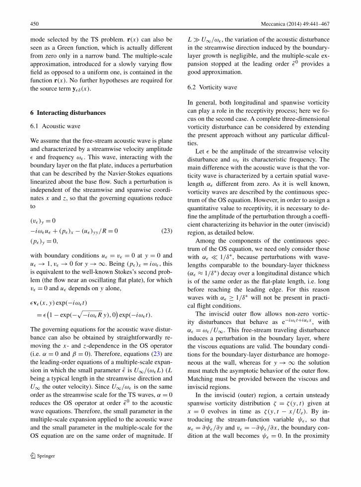
Fig. 1 Possible external disturbances inducing transition to tur-bulence in the boundary layer over a flat plate

= −pz + wxx + wyy + wzz

R,

together with the relevant initial and boundary con-ditions. Velocities are normalized with the outer ve-locity U∗∞ (a star ·∗ denoting dimensional quanti-ties, a hat · dimensionless ones), whereas the stream-wise, wall-normal and spanwise coordinates x, y andz are scaled with a typical boundary-layer thicknessδ∗

0 = √x∗

I ν∗/U∗∞ (x∗I being the first neutral point

of the neutral curve), and time with δ∗0/U∗∞. The

Reynolds number is defined as R = δ∗0U∗∞/ν∗ =

√x∗

I U∗∞/ν∗ =√

Rex∗I.

Referring to Fig. 1, we consider a general steady,incompressible boundary layer past a flat plate. Somedisturbances can originate in the external flow (acous-tic and vorticity waves), others at the wall (wall vi-bration and wall roughness). Following what was al-ready done by others [17, 19], we introduce two smalldisturbances εvε(x, y, z)e−iωε t and δvδ(x, y, z)e−iωδ t ,where vε = (uε, vε,wε) and vδ = (uδ, vδ,wδ) are re-spectively an unsteady wave of amplitude ε generatedby a general unsteady excitation source behaving ase−iωε t , and an unsteady wave of amplitude δ due toanother general unsteady excitation source behavingas e−iωδ t . These two perturbations are superimposedto a steady base flow V(x, y, z). Their interaction gen-erates beat waves, respectively

εδv+εδ(x, y, z)e−i(ωε+ωδ)t and

εδv−εδ(x, y, z)e−i(ωε−ωδ)t

at order εδ, plus other waves at higher orders. Thewavelength and frequency of the waves at orders ε

and δ, in general, are different from those typicalof TS waves. Their interaction at order εδ, however,

Meccanica (2014) 49:441–467 445

could generate a resonant wave. If we assume thatthe latter is εδv+

εδ(x, y, z)e−i(ωε+ωδ)t , allowing oneof the interacting frequencies to be negative, thenits amplitude is much larger than the amplitude ofεδv−

εδ(x, y, z)e−i(ωε−ωδ)t , which can be neglected. Thevelocity field inside the boundary layer v(x, y, z, t ) isthus decomposed into different contributions originat-ing from the steady base flow (V), from different en-vironmental sources (vε and vδ) and from their mutualinteraction (vεδ),

v(x, y, z, t ) = V(x, y, z) + εvε(x, y, z)e−iωε t

+ δvδ(x, y, z)e−iωδ t

+ εδvεδ(x, y, z)e−i(ωε+ωδ)t

+O(ε2) +O

(δ2) + · · · , (2)

where vεδ is understood as v+εδ . Of course, as a partic-

ular case one of the two frequencies might be zero.If the velocity decomposition (2) is substituted in

the Navier-Stokes equations (1), and the latter are suit-ably expanded, one finds three linear problems at or-ders ε, δ and εδ.

Linearization can also be applied to the boundaryconditions at the wall. In the case of wall roughness,the wall shape is expressed as δh(x), where δ is thetypical wall-roughness scale and h(x) is an order-onefunction of the streamwise coordinate. This distur-bance is stationary, and thus ωδ = 0.

On the other hand, wall vibration can generate anunsteady motion of the wall in the streamwise, span-wise or wall-normal direction. In the first two cases theproblem reduces to the well-known flow near an oscil-lating flat plate (Stokes’s second problem [58]), whilein the second one the position of the wall as a func-tion of time can be described by εe−iωε t where ε isthe typical amplitude of the vibration with a character-istic frequency ωε . If both disturbances (wall rough-ness and wall vibration) are acting at the wall, the wallshape must be described by the function H(x, t) =δh(x) + εe−iωε t .

In Appendix C we prove that wall vibration cou-pled with wall roughness does not lead to resonance.This allows us to consider the effect of wall rough-ness alone, which reduces the wall shape H(x, t) tothe steady form H(x) = δh(x).

Boundary conditions defined at y = δh(x) can beshifted to y = 0 via linearization because δ is a small

parameter. The Taylor expansion of the velocity fieldv about the position y = 0 leads to

v(x, y, z, t ) = v(x,0, z, t) + δh(x)∂ v(x, y, z, t )

∂y

∣∣∣∣y=0

+ 1

2δ2h2(x)

∂2v(x, y, z, t )

∂y2

∣∣∣∣y=0

+O(δ3) = 0. (3)

When the expansion (2) is introduced in the lineariza-tion (3), non-homogeneous boundary conditions orig-inate at order δ and εδ,

V(x,0, z) = 0

vε(x,0, z) = 0

vδ(x,0, z) = −h(x)∂V(x, y, z)

∂y

∣∣∣∣y=0

vεδ(x,0, z) = −h(x)∂ vε(x, y, z)

∂y

∣∣∣∣y=0

.

(4)

The system of linearized Navier-Stokes equationsand boundary conditions at the wall can now be for-mally and compactly written as

Lε(V,R)fε = yε (5)

Lδ(V,R)fδ = yδ (6)

Lεδ(V,R)fεδ = yεδ. (7)

Here fγ = (uγ , vγ , wγ , pγ ), with γ ∈ {ε, δ, εδ}, is thevector of unknowns while Lγ (V,R) is a linear opera-tor that depends on the base flow

V = (U (x, y, z), V (x, y, z), W (x, y, z)

)

and Reynolds number R. The right-hand-side (RHS)terms yγ (γ ∈ {ε, δ, εδ}) at orders ε and δ originatefrom the possible non homogeneous boundary condi-tions at the wall or at infinity (see conditions (4) at thewall). At order εδ, on the other hand, not only bound-ary conditions contribute to the RHS but also the cou-pling terms coming from the nonlinear part of the orig-inal Navier-Stokes equations, i.e. yεδ = −[0, a, b, c]T ,

446 Meccanica (2014) 49:441–467

with

a = uε(uδ)x + uδ(uε)x + vε(uδ)y

+ vδ(uε)y + wε(uδ)z + wδ(uε)z

b = uε(vδ)x + uδ(vε)x + vε(vδ)y

+ vδ(vε)y + wε(vδ)z + wδ(vε)z

c = uε(wδ)x + uδ(wε)x + vε(wδ)y

+ vδ(wε)y + wε(wδ)z + wδ(wε)z.

(8)

It should be noticed that equation (7) has to be satisfiedunder resonant conditions and thus requires additionalcare.

4 Non-homogeneous multiple-scale theory appliedto a one-dimensional resonant problem

In order to explain the use of multiple scales for thenon homogeneous and resonant problem (7), let usfocus on a simple time-dependent (one-dimensional)system.

As known from the study of the harmonic os-cillator driven by a sinusoidal forcing, x + ω2

0x =F0 cosωt , in the limit ω → ω0, i.e. under resonantconditions, the particular solution xp(t), induced bythe non-homogeneous source, can be rewritten asF0t sin(ω0t)/(2ω0). This expression emphasizes thepresence, in the case of undamped oscillations, of asecular term that grows indefinitely (and linearly) withtime for t → ∞.

On the other hand, if an oscillator (or anothermodel of a physical phenomenon) shows a separa-tion of scales, for instance in time, multiple scalescan efficiently account for it through the introductionof a small parameter ε that leads to the definition ofa new “slow” variable T = εt (see Appendix A fora simple, one-dimensional and homogeneous formu-lation). When multiple scales are employed for thestudy of resonant problems, the presence of the secularterm proportional to t leads to a solution that behavesas T/ε and still grows in time, but that provides anO(1/ε) effect. Two choices are available for introduc-ing the resonant forcing at the correct order in ε. If thefundamental order in the multiple-scale expansion is1/ε, then the resonant forcing should be introduced atorder ε0; if the leading order is ε0, as in the multiple-scale theory here presented, then the forcing term must

be multiplied by ε1. Under these assumptions, a time-dependent linear system forced to resonant conditionsreads

H (t)dx(t)

dt+ A(t)x(t) = εy(t), (9)

where matrices H and A are slowly varying with timet , x is the state vector, ε is, as noticed, the small param-eter that accounts for the slow variation with respect tot , and y is the resonant forcing term, appearing at orderε for the reason explained above.

The solution x is assumed to be representable in theform

x(t) = f(T ) exp(φ(T )/ε

)

= (f0(T ) + εf1(T ) + ε2f2(T ) + · · · )

× exp(φ(T )/ε

),

where the exponential is a fast varying oscillatingfunction, while vector f(T ) is the slowly varying partand is expanded in series of the small parameter ε. Un-der resonant conditions, on the other hand, the forcingy(t) is also fast varying, and can be expressed as

y(t) = (y0(T ) + εy1(T ) + ε2y2(T ) + · · · )

× exp(ψ(T )/ε

).

After expressing the derivative with respect to t interms of T (see Appendix A) and introducing it in theoriginal system (9), by separating the contributions atdifferent orders with respect to ε the following hierar-chy of linear systems is obtained,

ε0(

dφ

dTH (T )f0(T ) + A(T )f0(T )

)e

φ(T )ε = 0

ε

(dφ

dTH (T )f1(T ) + df0

dT+ A(T )f1(T )

)e

φ(T )ε

= εy0(T )eψ(T )

ε

... = ...

εn

(dφ

dTH (T )fn(T ) + dfn−1

dT+ A(T )fn

)e

φ(T )ε

= εnyn−1(T )eψ(T )

ε .

(10)

The homogeneous system at order zero (ε0) is a gen-eralized eigenvalue problem[A(T ) + λk(T )H (T )

]uk(T ) = 0 (11)

Meccanica (2014) 49:441–467 447

where λk(T ) = φ′(T ) is the eigenvalue anduk(T ) = f0(T ) is the right eigenvector. The latter isnot unique, i.e. f0(T ) = uk(T ) = ck(T )uk(T ), whereck(T ) is a multiplicative function and uk(T ) is theright eigenvector arbitrarily normalized.

At any other order, terms proportional to eψ(T )−φ(T )

ε

arise at the RHS when dividing by eφ(T )

ε . However,under resonant conditions ψ ′(T ) = φ′(T ) = λk(T ) sothat the system to be solved at order ε is

[A(T ) + λk(T )H (T )

]f1(T ) = −df0

dT+ y0(T ), (12)

which is linear, non homogeneous, but singular be-cause the coefficient matrix [A(T ) + λk(T )H (T )] isthe same as order ε0. For this reason the RHS mustsatisfy the compatibility condition, i.e. the dot productbetween the RHS and the left eigenvector vk , corre-sponding to the eigenvalue λk that renders the systemsingular, has to be zero:

vk(T ) ·(

−df0

dT+ y0(T )

)= 0. (13)

By expanding the compatibility condition (13) and re-calling that f0(T ) = ck(T )uk(T ), the following first-order non-homogeneous ordinary differential equationfor the unknown ck(T ) is derived

vk(T ) · uk(T )dck

dT+ vk(T ) · duk(T )

dTck

= vk(T ) · y0(T ). (14)

After introducing

p(T ) =[

vk(T ) · duk(T )

dT

]/[vk(T ) · uk(T )

]

and

q(T ) = [vk(T ) · y0(T )][vk(T ) · uk(T )] ,

equation (14) reduces to

dck

dT+ p(T )ck = q(T ),

whose closed-form solution is

ck(T ) = e− ∫ T

T0p(T ′) dT ′ ∫ T

T0

q(T ′′) e

∫ T ′′T0

p(T ′) dT ′dT ′′

=∫ T

T0

q(T ′′) e

∫ T ′′T p(T ′) dT ′

dT ′′.

Once ck(T ) is known, vector f0(T ) = ck(T )uk(T ) isretrieved. It should be noticed that f0(T ) is indepen-dent of the normalization chosen for uk(T ). By trun-cating the solution at order ε0, the state vector x(T ) isfinally obtained as x(T ) = ck(T )uk(T ) exp(φ(T )/ε)+O(ε) or, after substituting the closed-form expressionfor ck(T ),

x(T ) = uk(T )

∫ T

T0

[r(T ′′) ·y0

(T ′′)]dT ′′ +O(ε), (15)

where

r(T ′′) = vk(T

′′)eφ(T )

ε

vk(T ′′) · uk(T ′′)

× exp

(∫ T ′′

T

vk(T′) · duk(T

′)/dT

vk(T ′) · uk(T ′)dT ′

).

Equation (15) compactly expresses the state vector xas a function of the right eigenvector uk (computed atorder ε0 and arbitrarily normalized) multiplied by theintegral of the dot product between the resonant forc-ing source y0 and a weight r. The latter function, r, isotherwise known as “receptivity” because it describesthe sensitivity of the solution to the forcing y0. r con-tains the left eigenvector vk of the eigenvalue prob-lem (11), and therefore can be interpreted also as thesolution of the adjoint problem derived from (11).

5 Non-homogeneous multiple scales applied to thelinearized Navier-Stokes equations

The necessity to solve the resonant problem governedby equation (7) and the slow dependence of the linearoperator Lεδ on the streamwise coordinate suggest theuse of the multiple scales.

A small parameter ε, accounting for the scale sep-aration between the streamwise variation of the baseflow and the streamwise oscillation of the perturbationcan be introduced in a number of ways. If the scaleof the oscillation is assumed to be comparable to theboundary-layer thickness, it may seem natural to iden-tify ε with R−1/2. However, doing so leads to an in-viscid leading-order problem, which turns out to benon-uniformly valid across the boundary layer. This

448 Meccanica (2014) 49:441–467

non-uniformity is accounted for in multiple-deck the-ory, which eventually shows that ε is not O(R−1/2).

In a different approach, which we adopt here, ε

and R are treated as mutually independent parameters.This is actually the case if the base flow is embedded ina larger class of problems, possibly including volumeforces. In such a larger class of problems the stream-wise and normal scales of variation of the base floware untied to the Reynolds number (for instance, in atruly parallel flow the streamwise scale is infinite de-spite both the normal scale and Reynolds number arefinite), whereas the perturbation wavelength is a com-plicated function of the Reynolds number which is im-plicitly accounted for by keeping all the R-dependentterms in the equations, just as would happen in trulyparallel flow. The expansion parameter ε is the ra-tio between this wavelength and the typical longitu-dinal scale of the base flow. Of course the accuracy ofthe solution cannot be harmed by keeping all the R-dependent terms in the equations while performing anexpansion in ε only.

With a, b, c being the forcing terms as definedin (8), system (7) can be expanded similarly to (16).

(uεδ)x + (vεδ)y + (wεδ)z = 0

(uεδ)t + U (uεδ)x + uεδUx + V (uεδ)y + vεδUy

+ W (uεδ)z + wεδUz

= −(pεδ)x + R−1[(uεδ)xx + (uεδ)yy + (uεδ)zz]

− εa

(vεδ)t + U (vεδ)x + uεδVx + V (vεδ)y + vεδVy

+ W (vεδ)z + wεδVz (16)

= −(pεδ)y + R−1[(vεδ)xx + (vεδ)yy + (vεδ)zz]

− εb

(wεδ)t + U (wεδ)x + uεδWx + V (wεδ)y + vεδWy

+ W (wεδ)z + wεδWz

= −(pεδ)z + R−1[(wεδ)xx + (wεδ)yy + (wεδ)zz]

− εc.

It should be noted that the forcing terms appear multi-plied by ε, as explained for the one-dimensional reso-nant example in Sect. 4. Boundary conditions for sys-tem (16), which are derived from (4), provide a contri-

bution of order ε and read

uεδ(x,0, z) = −εh(x)∂uε

∂y|y=0

vεδ(x,0, z) = −εh(x)∂vε

∂y|y=0 (17)

wεδ(x,0, z) = −εh(x)∂wε

∂y|y=0.

Following the same steps as in the one-dimensionalexample (see Sect. 4 or the Appendix B), new coordi-nates are introduced, x = εx, y = y, z = εz, t = t andthe base flow is expressed in the new reference frameas

U(x,y, z) = U (x, y, z)

V (x, y, z) = V (x, y, z)/ε

W(x, y, z) = W (x, y, z).

The generic quantity q(x, y, z, t ) (which correspondsto u, v, w or p previously introduced) is expanded as

q(x, y, z, t ) = (q0(x, y) + εq1(x, y)

+ · · · )eiθ(x)

ε+iβz−iωt , (18)

where θ(x) is related to the streamwise wavenumberα by α = dθ/dx, β is the spanwise wavenumber andω the frequency. After introducing expression (18) to-gether with its first and second derivatives in (16) andboundary conditions (17), the original resonant prob-lem (7) is recast as two linear problems at orders ε0

and ε1 (in the multiple-scale small parameter ε),

order ε0:A(α,ω,R)f0εδ = 0

order ε1:

A(α,ω,R)f1εδ = −H (α,R)df0εδ

dx

+ C(α,R)f0εδ + yεδ,

(19)

where vectors

f0εδ = [u0εδ(x, y), v0εδ(x, y),w0εδ(x, y),p0εδ(x, y)

]

and

f1εδ = [u1εδ(x, y), v1εδ(x, y),w1εδ(x, y),p1εδ(x, y)

]

Meccanica (2014) 49:441–467 449

are the unknowns of the problem, and matrices A,H and C are defined in Appendix B (A is the well-known Orr–Sommerfeld operator). In what follows,vectors and matrices will be indicated as a functionof x only, even though they do depend on y as well.Equations (19) are the generalization of (11) and (12)to a multi-dimensional problem.

The order-0 equation in system (19) is the classi-cal Orr–Sommerfeld problem for the spatial-stabilityanalysis. Given ωTS and R, the wavenumber αTS of themost unstable mode (TS wave) and its correspondingeigenvector f0εδ are obtained from the dispersion rela-tion D(α,ω,R) = 0, which is equivalent to imposingdet(A) = 0. As noticed in Sect. 4, f0εδ is not uniqueand its normalization is arbitrary, i.e. f0εδ = c(x)f0εδ ,where c(x) is an unknown multiplicative function tobe determined through the solvability condition at or-der ε1.

At order ε1, the forcing yεδ has, in general, a widespectrum and therefore does not need to be representedby wave packets. However, since we are interested inthe resonant problem for which the wavenumber andfrequency of the forcing tend to the TS ones, we as-sume that the velocity disturbances at orders ε and δ

are in the form

ε[uε(x, y), vε(x, y),wε(x, y)

]

× exp

(i

∫αεdx′ − iωεt

)

and

δ[uδ(x, y), vδ(x, y),wδ(x, y)

]

× exp

(i

∫αδdx′ − iωδt

),

so that their coupling at order εδ provides the forcing

yεδ = −

⎛

⎜⎜⎝

0iαδuεuδ + iαεuδuε + vε(uδ)y + vδ(uε)y + iβwεuδ + iβwδuε

iαδuεvδ + iαεuδvε + vε(vδ)y + vδ(vε)y + iβwεvδ + iβwδvε

iαδuεwδ + iαεuδwε + vε(wδ)y + vδ(wε)y + iβwεwδ + iβwδwε

⎞

⎟⎟⎠ . (20)

The compatibility condition required to solve thesingular system at order ε1 in (19) provides the equa-tion for c

dc

dx+ a2

a1c = f∗ · yεδ

a1,

similar to (14), where a1 = f∗ · H f0εδ and a2 = f∗ ·Hd f0εδ/dx+C f0εδ . The solution at a final streamwiselocation xf is

c(xf) =∫ xf

x0

[f∗(x) · yεδ(x)

a1(x)

× exp

(−

∫ xf

x

a2(x′)

a1(x′)dx′

)]dx,

where x0 is a certain initial (upstream) station. Co-efficient a2 accounts for the non-parallel effects. Inthe case of parallel-flow assumptions (U = U(y) andV = W = 0) a2 is zero because d f0εδ/dx = 0 (thevector f0εδ is constant), and matrix C = 0 (it con-

tains the derivatives of U with respect to x and theV -component of the base flow).

By considering only the O(ε0) contribution to themultiple-scale expansion, the solution at order εδ isfεδ(xf) = c(xf)f0εδ(xf) exp(i

∫ xfx0

α dx′) +O(ε), or, af-ter substituting c(xf),

fεδ(xf) = f0εδ(xf)

∫ xf

x0

r(x) · yεδ(x) dx +O(ε), (21)

with

r(x) = f∗(x)

a1(x)× e

i∫ xfx0

α dx′−∫ xfx

a2a1

dx′. (22)

Vector fεδ in (21) includes the eigenvector f0εδ at or-der ε0 and the integral of the dot product between theresonant forcing yεδ(x) and the vector r(x), which isthe receptivity (sensitivity) of the solution to the forc-ing. It should be kept in mind that the solution fεδ(xf),in general, is expressed by a convolution and not by asimple integral. The simplification to an integral orig-inates from the fact that we are focusing on a specific

450 Meccanica (2014) 49:441–467

mode selected by the TS problem. r(x) can also beseen as a Green function, which is actually differentfrom zero only in a narrow band. The multiple-scaleapproximation, introduced for a slowly varying flowfield as opposed to a uniform one, is contained in thefunction r(x). No further hypotheses are required forthe source term yεδ(x).

6 Interacting disturbances

6.1 Acoustic wave

We assume that the free-stream acoustic wave is planeand characterized by a streamwise velocity amplitudeε and frequency ωε . This wave, interacting with theboundary layer on the flat plate, induces a perturbationthat can be described by the Navier-Stokes equationslinearized about the base flow. Such a perturbation isindependent of the streamwise and spanwise coordi-nates x and z, so that the governing equations reduceto

(vε)y = 0

−iωεuε + (pε)x − (uε)yy/R = 0 (23)

(pε)y = 0,

with boundary conditions uε = vε = 0 at y = 0 anduε → 1, vε → 0 for y → ∞. Being (pε)x = iωε , thisis equivalent to the well-known Stokes’s second prob-lem (the flow near an oscillating flat plate), for whichvε = 0 and uε depends on y alone,

εvε(x, y) exp(−iωεt)

= ε(1 − exp(−√−iωεR y),0

)exp(−iωεt).

The governing equations for the acoustic wave distur-bance can also be obtained by straightforwardly re-moving the x- and z-dependence in the OS operator(i.e. α = 0 and β = 0). Therefore, equations (23) arethe leading-order equations of a multiple-scale expan-sion in which the small parameter ε is U∞/(ωεL) (Lbeing a typical length in the streamwise direction andU∞ the outer velocity). Since U∞/ωε is on the sameorder as the streamwise scale for the TS waves, α = 0reduces the OS operator at order ε0 to the acousticwave equations. Therefore, the small parameter in themultiple-scale expansion applied to the acoustic waveand the small parameter in the multiple-scale for theOS equation are on the same order of magnitude. If

L � U∞/ωε , the variation of the acoustic disturbancein the streamwise direction induced by the boundary-layer growth is negligible, and the multiple-scale ex-pansion stopped at the leading order ε0 provides agood approximation.

6.2 Vorticity wave

In general, both longitudinal and spanwise vorticitycan play a role in the receptivity process; here we fo-cus on the second case. A complete three-dimensionalvorticity disturbance can be considered by extendingthe present approach without any particular difficul-ties.

Let ε be the amplitude of the streamwise velocitydisturbance and ωε its characteristic frequency. Themain difference with the acoustic wave is that the vor-ticity wave is characterized by a certain spatial wave-length αε different from zero. As it is well known,vorticity waves are described by the continuous spec-trum of the OS equation. However, in order to assign aquantitative value to receptivity, it is necessary to de-fine the amplitude of the perturbation through a coeffi-cient characterizing its behavior in the outer (inviscid)region, as detailed below.

Among the components of the continuous spec-trum of the OS equation, we need only consider thosewith αε � 1/δ∗, because perturbations with wave-lengths comparable to the boundary-layer thickness(αε ≈ 1/δ∗) decay over a longitudinal distance whichis of the same order as the flat-plate length, i.e. longbefore reaching the leading edge. For this reasonwaves with αε ≥ 1/δ∗ will not be present in practi-cal flight conditions.

The inviscid outer flow allows non-zero vortic-ity disturbances that behave as e−iωε t+iαεx , withαε = ωε/U∞. This free-stream traveling disturbanceinduces a perturbation in the boundary layer, wherethe viscous equations are valid. The boundary condi-tions for the boundary-layer disturbance are homoge-neous at the wall, whereas for y → ∞ the solutionmust match the asymptotic behavior of the outer flow.Matching must be provided between the viscous andinviscid regions.

In the inviscid (outer) region, a certain unsteadyspanwise vorticity distribution ζ = ζ(y, t) given atx = 0 evolves in time as ζ(y, t − x/Ue). By in-troducing the stream-function variable ψε , so thatuε = ∂ψε/∂y and vε = −∂ψε/∂x, the boundary con-dition at the wall becomes ψε = 0. In the proximity

Meccanica (2014) 49:441–467 451

of the wall, the solution behaves (in y) as ψε(y) = Cy

where C = f (t − x/Ue) or, in Fourier components,C = eiωε(t−x/Ue). If we limit our analysis to distur-bances of wavelengths much larger than the boundary-layer thickness, then this is precisely the behavior thatwe expect at the matching with the outer solution, andallows us to assign a certain intensity to the pertur-bation as a function of the coefficient C, which is, in-deed, the velocity of the outer (inviscid) flow evaluatedat the wall. It should be noted that, in order to providea quantitative value of receptivity (which must be in-dependent of multiplicative constants), it is necessaryto assign the intensity of the perturbation through awell-determined property of the outer solution.

As an alternative to the linearized boundary-layerequations, the matching with the viscous region canemploy the Orr-Sommerfeld equation (more suitablefor the present analysis). The solutions of the OS equa-tion corresponding to the continuous spectrum, in thelimit y → ∞, are unique up to a multiplicative con-stant for every pair (ω,α). Such solutions contain theterms

e(−αy), e√

α2+iR(αUe−ω)y,

e−√

α2+iR(αUe−ω)y

in certain proportions and, therefore, can behave dif-ferently as y → ∞. Also the solutions of the linearizedboundary-layer equations are unique up to a multi-plicative constant, contain the terms

1, e√

iR(αUe−ω)y, e−√iR(αUe−ω)y,

and, for the same reasons as for the OS solutions, canbehave differently as y → ∞.

The dispersion relation of the outer-region wavesmust now be considered. For the OS equation, theouter dispersion relation α2 + iR(αUe − ω) = 0 en-sures that the solution behaves (in y) as C1 + C2y +C3e−αy , (whereas for the boundary-layer equationsthe condition αUe − ω = 0 implied that the solutionbehaves as C1 + C2y + C3y

2). In both cases it is pos-sible to normalize the solution such that C2 = 1. In-deed, this is always true for the boundary-layer case,whereas for the OS case, in general, a wave packet de-pending also on the spanwise wavenumber β shouldbe considered. However, since a disturbance can reachthe leading edge before decaying only if β is small,the present analysis (β = 0) is satisfactory.

We consider the OS approach and compute thewavenumber of the vorticity wave from the outer dis-persion relation α2 + iR(αUe − ω) = 0 as

αε = −iUe + i√

U2e − 4iωεR−1

2R−1. (24)

Having set C2 = 1, the asymptotic solution becomes

ψε = (C1 + y + C3e−αεy

)ei(αεx−ωεt),

which implies:

uε = ∂ψε

∂y= (

1 − αεC3e−αεy)ei(αεx−ωεt)

vε = −∂ψε

∂x= −iαε

(C1 + y + C3e−αεy

)ei(αεx−ωεt).

The boundary conditions for y → ∞, therefore, re-duce to

uε → (1 − αεC3e−αεy

)ei(αεx−ωεt)

vε → −iαε

(C1 + y + C3e−αεy

)ei(αεx−ωεt),

(25)

with C1 and C3 free constants. It should be noted thatall of the above analysis serves only the purpose of as-signing a precise value to the multiplicative constant,whereas the behavior for y → ∞ is a priori deter-mined by the OS solution corresponding to the con-tinuous spectrum.

The governing equations for the vorticity wave arethe same as for the OS problem, with conditions (25)replacing the classical homogeneous boundary con-ditions at infinity. This is equivalent to solving theleading-order equations of the multiple-scale expan-sion. The condition that guarantees a good approxima-tion at the leading order ε0 is L � U∞/ωε , where L isthe typical streamwise length on which the boundarylayer evolves and U∞/ωε = 1/αε is the typical lengthon which the vorticity perturbation evolves.

Contrary to the OS case, however, the problem isnonsingular because αε and ωε are not simultaneouslyαTS and ωTS. After discretization, the governing equa-tions and boundary conditions can formally be writtenas A(αε,ωε,R)fε(x) = yε(x) exp(i

∫αε dx′), where

A is the OS operator, fε(x) is the solution as a func-tion of x (the y-dependence has already been consid-ered in the discretization), and yε(x) accounts onlyfor the non homogeneous boundary conditions at in-finity (25). The vorticity-wave velocity disturbance is

452 Meccanica (2014) 49:441–467

ultimately expressed as

εvε(x, y) exp(−iωεt)

= ε(uε(y), vε(y)

)exp

(i

∫αε dx′ − iωεt

).

6.3 Wall roughness

The wall-roughness shape is described by a func-tion y = δh(x), where δ is the typical roughnessscale and h(x) is an order-one function. In principle,when decomposed in Fourier series, h(x) has a widewavenumber spectrum. However, resonance betweenthe TS wave and the nonlinear mixing of disturbancesoccurs only for a specific value of the wall-roughnesswavenumber. Therefore, we focus on a particular αδ ,keeping in mind that the analysis can be performed fordifferent wavenumbers.

We express the steady perturbation induced in theboundary layer by the wall roughness as a wave in theform (u(x, y), v(x, y),w(x, y))ei

∫αδ dx′

, where αδ isrelated to the inverse of the typical roughness wave-length. The governing equations can be obtained fromthe multiple-scale approximation limited to the lead-ing order ε0. A good approximation is provided aslong as L � 1/αδ , where L is the scale of boundary-layer variation and 1/αδ is the scale on which the wall-roughness induced perturbation varies. Formally, theOS operator is employed, but the problem is solvedfor ωδ = 0 (the perturbation is steady) and with non-homogeneous boundary conditions originating fromthe linearization at the wall:

u0δ(x,0) = −h(x)∂U

∂y

∣∣∣∣y=0

e−i∫

αδ dx′

v0δ(x,0) = −h(x)∂V

∂y

∣∣∣∣y=0

e−i∫

αδ dx′

w0δ(x,0) = −h(x)∂W

∂y

∣∣∣∣y=0

e−i∫

αδ dx′.

After the discretization of the equations and boundaryconditions, the problem at order δ reduces to the linearsystem A(αδ,0,R)fδ(x) = yδ(x)h(x) exp(−i

∫αδ dx′),

where A is the OS operator evaluated at α = αδ

and ω = 0, fδ(x) is the solution as a function of x

(the y-dependence has already been considered inthe discretization), and yδ(x) is nonzero only be-cause of the terms −(∂U/∂y)|y=0, −(∂V/∂y)|y=0 and−(∂W/∂y)|y=0 stemming from the boundary condi-tions at the wall.

6.4 Possible disturbance interactions

The disturbances modeled in the previous sectionscannot resonate singularly with TS waves. For exam-ple, the wavenumber of an acoustic wave, in the in-compressible case, is zero and thus it can never beclose to αTS (the frequency, however, could be in therange of ωTS). The same happens for the wall vibra-tion disturbance, for which α = 0. Vorticity waves, onthe other hand, are perturbations characterized by bothwavenumber and frequency different from zero; how-ever α = ω/U∞ is far from αTS. Wall roughness, be-ing stationary, cannot excite TS waves, at least as longas swept wings are not considered.

On the other hand, a resonant wave with wavenum-ber and frequency in the TS range can originate at or-der εδ, via nonlinear interaction between the distur-bances at orders ε and δ. Resonance conditions requireαδ +αε ≈ αTS and ωδ +ωε ≈ ωTS, so that only specificcoupling between perturbations can effectively satisfythem. Possible interesting interactions are the follow-ing.

– Acoustic wave and wall roughness. The acousticwave is solved at order ε and the wall roughnessat order δ. αε = 0 and ωδ = 0, so that resonance isguaranteed by αδ ≈ αTS and ωε ≈ ωTS. The bound-ary conditions to be used at the wall, after the lin-earization, are (4), which at order εδ include the firstderivative of the Stokes’s solution at the wall.

– Vorticity wave and wall roughness. The vorticitywave perturbation is computed at order ε and thewall roughness at order δ. Since the vorticity-wavedispersion relation allows αε �= 0 and ωε �= 0, reso-nance conditions are αδ + αε ≈ αTS and ωε ≈ ωTS.The correct boundary conditions at the wall are stilldescribed by the fourth equation in (4), so that thefirst derivative of the vorticity wave is employed atthe wall.

– Acoustic wave and vorticity wave. The acousticwave, solved at order δ, is characterized by αδ = 0and ωδ �= 0. The vorticity wave, on the contrary,allows both αε �= 0 and ωε �= 0, so that resonancecan occur if αε ≈ αTS and ωδ + ωε ≈ ωTS. Thecombination between acoustic and vorticity wavesprovides homogeneous boundary conditions at thewall.

A subsection of Appendix C is devoted to the in-teraction between wall roughness and wall vibration.

Meccanica (2014) 49:441–467 453

For this case, we prove that the velocity disturbance atorder εδ is the exact solution of the velocity perturba-tion induced by wall roughness on a wall vibrating inthe normal direction, after introducing a new referenceframe.

6.5 Wall receptivity coefficient

When the “tuning mechanism” that allows resonancewith TS waves is due to wall roughness, the am-plitude of the unstable perturbation can be relateddirectly to the wall shape h(x). Since the solutionat order δ is a linear function of h(x) (through theboundary conditions), so is the solution at order εδ.This allows us to rewrite the forcing vector yεδ ap-pearing in (19) at order ε as yεδ(x) = yεδ(x)h(x),where yεδ(x) = yεδ(x)/h(x). The integral in (21) be-comes

∫ xfx0

r(x)·yεδ(x) dx = ∫ xfx0

r(x)· yεδ(x)h(x) dx =∫ xfx0

rh(x)h(x) dx, where rh(x) is a scalar function de-noting the dot product r(x) · yεδ(x) (it should be keptin mind that vectors depend also on y, here omitted inorder to keep the notation lighter). Equation (21) cannow be recast in the following form, where the lineardependence on the wall shape h(x) is emphasized,

fεδ(xf) = f0εδ(xf)

∫ xf

x0

rh(x)h(x) dx +O(ε). (26)

The reduction to a simple integral occurs because weare focusing on a single mode selected by the TS wave.More generally, the exciting source yεδ(x), due tothe nonlinear interaction between wall roughness andother disturbances, can be written, using the Greenfunction g, as yεδ(x) = ∫ xf

x0g(x, x′)h(x′) dx′. The so-

lution fεδ , when employing g, is

fεδ(xf) = f0εδ(xf)

[∫ xf

x0

∫ xf

x0

r(x)g(x, x′)h

(x′)dx′ dx

]

× exp(−iωεt) +O(ε),

and therefore more complicated than the simple inte-gral (26).

By introducing the x-dependent coefficient

rh = f∗ · yεδ

a1= f∗ · yεδ

f∗ · [H f0εδ], (27)

and by recalling the definition of r(x) as in (22),a1 = f∗ · H f0εδ and a2 = f∗ · Hd f0εδ/dx + C f0εδ (seeSect. 5), the solution fεδ(xf) in (26) becomes

fεδ(xf) = f0εδ(xf)

×∫ xf

x0

rh(x) ei∫ xfx0

α dx′−∫ xfx

a2a1

dx′h(x)dx.

(28)

If the eigensolution f0εδ(xf) in (28) has beennormalized in such a way that max|u0εδ(xf)| = 1(f0εδ = [u0εδ, v0εδ, w0εδ, p0εδ]T), then the amplitudeof fεδ(xf) (defined as the maximum absolute value ofthe streamwise velocity component εδuεδ(xf, y) fory ∈ [0;+∞[) is

A(xf) =∣∣∣∣εδ e

i∫ xfx0

α dx′ ∫ xf

x0

h(x)rh(x)e− ∫ xf

x

a2a1

dx′dx

∣∣∣∣.

By introducing the receptivity coefficient

rh(x) = rh(x) e− ∫ xI

x

a2a1

dx′, (29)

the final amplitude A(xf) can be further rearranged toemphasize its dependence on the integral between thewall shape h(x) and the receptivity coefficient

A(xf) =∣∣∣∣εδe

i∫ xfx0

α dx′e− ∫ xf

xI

a2a1

dx′ ∫ xf

x0

h(x)rh(x) dx

∣∣∣∣.

(30)

Expression (30) is what we defined as the goal of a re-ceptivity study because the final amplitude of the res-onant wave A(xf) is formulated as a function of ε (theamplitude of the acoustic wave, vorticity wave or walldisplacement due to the wall vibration), δ (the ampli-tude of the wall roughness), and h(x) (the shape of thewall). An essential role is played by rh(x), which isthe receptivity to wall roughness or, in other words,the sensitivity of the final amplitude to the wall shapeh(x). Non-parallel flow effects in (30) are accountedfor by the integral of a2/a1 in the exponential factors,whereas for parallel flows (a2 ≡ 0) the amplitude (30)reduces to

Aparallel(xf) =∣∣∣∣εδ e

i∫ xfx0

α dx′ ∫ xf

x0

h(x)rh(x) dx

∣∣∣∣.

It should be noticed that rh(x) (see (27) for its def-inition) is the same receptivity coefficient computedfor parallel flows by Crouch [19], Choudhari andStreett [17] and Hill [36] (these comparisons were car-ried out during the code verification).

454 Meccanica (2014) 49:441–467

For the interaction between the acoustic and vor-ticity waves h(x) ≡ 0 and the wall boundary condi-tions are homogeneous at all orders (ε—vorticity waveperturbation, δ—acoustic wave perturbation, and εδ—resonant wave). The amplitude at the final station forthis interaction is

A(xf) = ∣∣εδei∫ xfx0

α dx′e− ∫ xf

xI

a2a1

dx′AI

∣∣,

where

AI =∫ xf

x0

f∗ · yεδ

a1e− ∫ xf

x

a2a1

dx′dx.

7 Results

In this section we present the results for Blasius’boundary layer and consider each interaction de-scribed in Sect. 6. We systematically provide per-turbations at order ε and δ, followed by the forcingterms originating from their interactions at order εδ.Only the x- and y-momentum contributions to the lefteigensolution f∗ and to the forcing yεδ are shown, be-cause they are the only effective (nonzero) terms inyεδ . The receptivity coefficient is eventually plottedversus Reynolds number R for both parallel and non-parallel flows.

The wall-normal coordinate is normalized with theboundary-layer reference length δ0 = √

νxI/U∞. Thereference Reynolds number is RI = U∞δ0/ν = 557,where R = √

Rex = √U∞x/ν. The dimensionless

frequency F = ων/U2∞ has been chosen as F = 5.9 ×10−5, because for this value the amplification reachesa maximum with respect to F .

7.1 Acoustic wave–wall roughness interaction

Figure 2a shows the perturbation induced by theacoustic wave that travels in the free stream. The v-component is identically zero, whereas the u-component,independent of x, is Stokes’s solution and becomesconstant for y/δ0 > 3. Therefore, the main contribu-tion of the acoustic perturbation to the forcing is con-fined within the boundary layer. Figure 2b reports theabsolute value of the perturbation induced by the wallroughness and computed at αδ = αTS. Its main con-tribution is clearly localized inside the boundary layertoo, with the solution going asymptotically to zero asy/δ0 → ∞. The y-scale of the plot is limited to 10

Fig. 2 Interacting perturbations at order ε and δ.F = ων/U2∞ = 5.9 × 10−5, RI = 557

in order to disclose the most relevant features, whichare significant only in the wall region, but the com-putations are performed for ymax/δ0 = 180 (an outerzoom is proposed in Sect. 7.2 for the coupling betweenvorticity wave and wall roughness).

The interaction at order εδ between the previousperturbations produces the x- and y-momentum forc-ing terms reported in Fig. 3a (in absolute value). Thestrongest effect is provided by the x-momentum com-ponent, which is mainly localized inside the bound-ary layer, as a direct consequence of the perturbationsshown in Fig. 2. It should be kept in mind that, at or-der εδ, a contribution to the forcing comes also fromthe non homogeneous boundary condition at the wall.This contribution is not shown in Fig. 3a because thewhole plot would not be visible due to the differentorders of magnitude.

Meccanica (2014) 49:441–467 455

Fig. 3 Interaction between acoustic wave and wall roughnessat order εδ. F = ω/(νU2∞) = 5.9 × 10−5, RI = 557

The absolute value of the left eigenfunction f∗is reported in Fig. 3b. The x- and y-momentumcontributions, which weight respectively the x- andy-momentum forcing, reach their maxima for y/δ0 <

5 suggesting that the receptivity coefficient originatingfrom f∗ · yεδ might be quite large.

This conjecture is confirmed by Fig. 4a, where theabsolute value of the receptivity coefficient is plot-ted under the assumptions of parallel and non par-allel flows. In both cases it monotonically decreaseswith R. For parallel flows the coefficient reduces torh = f∗ · yεδ/a1, which can be directly compared withthe results carried out by Crouch [19], Choudhari andStreett [17] and Hill [36]. For non parallel flows thereceptivity coefficient is rh = rh exp(− ∫ xI

xa2a1

dx′),where a2 �= 0 accounts for non-parallel effects. Since

Fig. 4 Receptivity characteristics for the interaction betweenacoustic wave and wall roughness. F = ων/U2∞ = 5.9 × 10−5,RI = 557

the integral in rh is referred to the first neutral point,the values of the receptivity coefficients coincide atRI = 557.

In order to better appreciate the contributionof the multiple scales in accounting for the boundary-layer growth, Fig. 4b shows the ratio rh/rh =exp(− ∫ xI

xa2a1

dx′) between the non-parallel and par-allel cases. Differences are on the order of 10 %, withpeaks of 15 %, meaning that non-parallel flow effectsintroduced by this formulation play a non-negligiblerole even in Blasius’ boundary layer. It should be no-ticed that for F = ων/U2∞ = 5.9 × 10−5 non-paralleleffects are not as strong as at higher frequencies (e.g.F = 22 × 10−5). For a more detailed discussion onnon-parallel effects see Sect. 8.

456 Meccanica (2014) 49:441–467

Fig. 5 Interacting perturbations. F = ων/U2∞ = 5.9 × 10−5,RI = 557

7.2 Vorticity wave–wall roughness interaction

The perturbation induced by a vorticity wave, at thefirst neutral point, is plotted in Fig. 5a. For the con-ditions considered (F = 5.9 × 10−5 and RI = 557),the wavenumber of TS waves (normalized with δ0)is αTSδ0 = 0.1. The value of the spatial wavenumber,αεδ0 = 0.0329, to be used for the computation of thevorticity wave perturbation, is provided by (24). Thewavenumber of the wall roughness perturbation is thusαδδ0 = αTSδ0 − αεδ0 = 0.067.

Figure 5a reveals that a very large value of y/δ0 isrequired to achieve the asymptotic values of u and v.As y/δ0 → ∞, the u-component reaches a constantvalue equal to 1 and the v-component behaves as alinear function of y/δ, as imposed by the boundaryconditions (25). The main contribution of the vortic-

Fig. 6 Interaction between vorticity wave and wall roughnessat order εδ. F = ω/(νU2∞) = 5.9 × 10−5, RI = 557

ity wave perturbation is outside the boundary layer,as it was observed by Wu [65], confirming the “shearsheltering” mechanism described by Hunt [37]. Onthe contrary, the perturbation due to wall roughness,which is reported in Fig. 5b, is mainly localized insidethe boundary layer (this figure differs from Fig. 2b forthe choice of the wavenumber αδ).

The forcing terms caused by the interaction be-tween vorticity wave and wall roughness are shownin Fig. 6a. In contrast with the interaction betweenacoustic wave and wall roughness, here the forcingis mainly localized outside the boundary layer. Thex-momentum excitation peaks at about y/δ0 = 8,whereas the y-momentum reaches its maximum atabout y/δ0 = 20. This is clearly due to the behaviorof the velocity profiles induced by the vorticity wave,which do not go to zero as y/δ0 → ∞. The pertur-

Meccanica (2014) 49:441–467 457

Fig. 7 Receptivity characteristics for the interaction betweenvorticity wave and wall roughness. F = ων/U2∞ = 5.9 × 10−5,RI = 557

bation due to the wall roughness, on the contrary, ex-ponentially decays with the distance from the wall,driving the forcing term to zero as y/δ0 → ∞. Thisexponential decay of yεδ , however, is much slowerthan the decay observed for the interaction betweenan acoustic wave and wall roughness, so that a muchlarger distance from the wall is needed in order for itto vanish. The left eigenfunction f∗ in Fig. 6b has thesame characteristics as that in Fig. 3b, except to they scale.

Parallel and non parallel receptivity coefficients arereported in Fig. 7. They monotonically decreases withR, just as in the acoustic wave–wall roughness in-teraction, and their ratio is the same as in Fig. 4b.Here, however, the slope of the curves is larger thanin the previous case and the absolute values of the co-efficients are about one order of magnitude smaller.Clearly, this is due to the fact that now the absolutevalue of the exciting terms in yεδ is one order of mag-nitude smaller than before, and to the fact that theforcing and the left eigenfunction peak at completelydifferent distances from the wall (compare Figs. 6aand 6b). This feature could lead us to think that theinteraction between vorticity wave and wall roughnessis a negligible phenomenon (shear sheltering [37]). Itcan be true, but the final amplitude has to be yet mul-tiplied by ε, the amplitude of the vorticity wave in thefree-stream, and δ, the amplitude of the wall rough-ness. Therefore, the relative importance of one phe-nomenon with respect to the other depends on the ac-tual level of the environmental disturbances involved.

Fig. 8 Interacting perturbations. F = ων/U2∞ = 5.9 × 10−5,RI = 557

7.3 Acoustic wave–vorticity wave interaction

As for the previous interactions, we consider F =5.9 × 10−5 and RI = 557 obtaining αTSδ0 = 0.1.Since resonance occurs at αε = αTS, the wavenum-ber for the vorticity wave is αε = 0.1 whereas itsfrequencyωε is computed from equation (24),ωε = (α2

ε + iαεUeR)/(iR). Resonance imposes alsoωε + ωδ = ωTS, that gives the frequency of the acous-tic wave ωδ = ωTS − ωε .

The velocity perturbation due to the acoustic waveis shown in Fig. 8a. It should be noticed that this isnot the same as in Fig. 2a because the frequency of theacoustic wave is different in the two cases. The gen-eral shape of the profile remains, however, unchanged.The vorticity wave perturbation in Fig. 8b shows a

458 Meccanica (2014) 49:441–467

Fig. 9 Interaction between acoustic wave and vorticity wave atorder εδ. F = ω/(νU2∞) = 5.9 × 10−5, RI = 557

quite remarkable difference compared with Fig. 5a. Inthe present case, the u-velocity component reaches theasymptotic value at y/δ0 ≈ 60, while u = 1 was previ-ously reached at y/δ0 ≈ 140 (Fig. 5a).

The nonlinear interaction between the two distur-bances of Fig. 8 is shown in Fig. 9a. The main differ-ence with the previous cases is that the forcing doesnot vanish for y/δ0 → ∞, as a consequence of theinteracting-disturbances profiles, but behaves almostas the vorticity wave perturbation (a part from thescale).

On the contrary, the left eigenfunction f∗ (Fig. 9b)reaches its maximum where the forcing term is verysmall and goes exponentially to zero where the forcingbehaves as a constant (x-momentum) or linearly (y-momentum). For this reason the effects of the forcingare very limited.

8 A brief discussion on non-parallel effects

As mentioned in the introduction (see Sect. 2), dur-ing the historical development of receptivity theory,approaches different from multiple scales have beenproposed in order to account for non-parallel ef-fects. Among those, PSE has been successfully em-ployed [1, 6, 35, 51] because this nonlinear partial dif-ferential equation incorporates the effects of stream-wise divergence associated with boundary-layer non-parallelism. The aim of this brief discussion is to provethat results here obtained with multiple scales (MS)including non-parallel effects agree with PSE (whenPSE converges) and other OS approaches.

Figure 10a reproduces Fig. 7 of Ref. [20], in whichthe OS formulation was employed and the hypothesisof parallel flow was relaxed by introducing the deriva-tive of the disturbance amplitude with respect to thestreamwise direction. The effective branch I ampli-tude AI is reported as a function of the wall-roughnesswavenumber αw for F = ων/U2∞ = 5.6 × 10−5, andR = 550 (these conditions are slightly different fromthose in Sect. 7). Full symbols refer to present cal-culations (MS), while empty symbols are data gath-ered from Ref. [20]. Only one point is, however, avail-able for the PSE, AI = 51.7 at αw = 0.174236. FromFig. 10a it is clear that the quasi-parallel-flow ap-proach introduced by Crouch [20] (empty squares)provides results that are much closer to the paral-lel, rather than non-parallel, computations carried outwith the present multiple-scale approach. More specif-ically, without non parallel corrections to the ampli-tude (parallel-flow case, full squares), the maximumerror is within 2.6 % and the optimal wavenumber αw

(for which the maximum of AI is achieved) is aboutαw = 0.1714, the same obtained by Crouch.

When non-parallel effects are accounted for (fullcircles in Fig. 10a), on the other hand, results differfrom the quasi-parallel-flow approach, but agree verywell with the values reported by Crouch [20] regard-ing the PSE, i.e. AI = 51.7 at αw = 0.174236. Unfor-tunately, from the data available in literature it is al-most impossible to gather enough information for re-constructing a curve to plot in Fig. 10a for the PSE.However, it can be concluded that non-parallel effectsinfluence the optimal αw but not the value of the max-imum AI, which is quite insensitive.

In Fig. 10b we compare MS and PSE by plottingthe N -factor (with non-parallel effects) as a function

Meccanica (2014) 49:441–467 459

Fig. 10 Comparison with previously published results account-ing for non-parallel effects. (a) Comparison with Crouch [20]:variation of the effective branch I amplitude AI with αw forF = ων/U2∞ = 5.6 × 10−5, R = 550. (b) Comparison withBertolotti et al. [6]: amplification curves as a function of R forF = ων/U2∞ = 22 × 10−5, where non-parallel effects are verystrong

of R for F = ων/U2∞ = 22 × 10−5, which representsthe worst-case scenario. In fact, Bertolotti et al. [6]showed that at high frequency non-parallel-flow ef-fects play a non-negligible role in the Blasius’ bound-ary layer (see Fig. 3a, p. 416, in Ref. [6]), whereas inthe usual range of frequencies (i.e. for F = 5 × 10−5),linear stability theory, PSE and DNS agree extremelywell (Fig. 3b, p. 416, in Ref. [6]). Therefore, results arehere compared directly at F = 22 × 10−5 for which,however, no direct comparison with DNS is avail-able. Figure 10b reports PSE results by Bertolotti etal. [6] (solid line) and the MS results computed withthe present method (dashed line), showing a verygood agreement, with a maximum error on the orderof 1.5 %.

This discussion suggests the potential of multiplescales as a promising tool to improve transition predic-tion methods, including receptivity calculations andnon-parallel effects. In fact, in addition to PSE, mul-tiple scales provide the correct representation of anarbitrary initial condition, a more satisfactory theory,and a simpler numerical implementation (no numeri-cal stability problems).

9 Comparison with three-dimensional results

In this section we compare our results, with or withoutnon-parallel flow corrections, with those obtained byCrouch [22] who studied the receptivity of a three-dimensional boundary layer to cross-flow vorticesin the parallel-flow framework. We consider the in-compressible three-dimensional boundary-layer flowover an infinite swept wing modeled using the two-parameter family of similarity solutions for yawedwedge flows given by Cooke [18]. The first param-eter, m, describes the intensity of the pressure gra-dient, whereas the second, Λ, is the sweep angle.The Hartree parameter βH = 2m/(1 + m), associatedwith a wedge angle of βH π/2, can be used instead ofm. Following [22], we consider the reference framex∗y∗x∗ such that x∗ is the chordwise coordinate (nor-mal to the leading edge), y∗ is normal to the wing(pointing upwards) and z∗ is the spanwise coordinate(parallel to the leading edge). The reference frame isset at a certain distance x∗

0 from the leading edge. IfQc denotes a constant free-stream velocity, then itscomponents normal and parallel to the leading edgeare, respectively,

Uc = Qc cosΛ and Wc = Qc sinΛ.

We introduce a reference length c∗ such that the globalReynolds number is Rc = √

(Qcc∗)/ν. All velocitiesare normalized with Qe and all lengths with

δr =√

ν(x∗0 + x∗)Ue

,

where Ue = UcXm is the chordwise velocity com-

ponent at the edge of the boundary layer and X =(x∗

0 +x∗)/c∗ is the normalized distance from the lead-ing edge. If We denotes the constant velocity compo-nent parallel to z∗ at the edge of the boundary layer,

460 Meccanica (2014) 49:441–467

We = Wc, then the total edge velocity Qe is

Qe(X) =√

U2e (X) + W 2

e

= Qc cosΛ√

X2m + tan2 Λ.

We introduce the normalized normal-wall coordinate

y = y∗

δr

= y∗√

Ue

ν(x∗0 + x∗)

such that the three boundary-layer velocities compo-nents normalized with Qe(X) are

U(X,y) = Ue(X)

Qe(X)f ′(y)

V (X,y) = Ue(X)

Qe(X)

1 − m

2

√ν

Ue(X)X

[yf ′(y)

− m + 1

1 − mf (y)

]

W(X,y) = We

Qe(X)g(y),

where f (y) and g(y) are the Falkner-Skan-Cooke(FSC) family of profiles solutions of the two differ-ential equations [18]

f ′′′ + m + 1

2ff ′′ + m

(1 − f ′2) = 0 (31)

g′′ + m + 1

2fg′ = 0 (32)

supplemented by the boundary conditions

f (0) = f ′(0) = g(0) = 0 and f ′(∞) = g′(∞) = 1.

Hereafter we focus on the same conditions used byCrouch [22]:

Rc = 1000, Λ = 30◦, βH = 0.6.

The dimensionless Navier-Stokes equation depend onthe local Reynolds number

R = Qeδr

ν,

which is related to the global Reynolds number Rc bythe equation

R = R2c

Qe

Qc

X

x0 + x= R2

c

Qe

Qc

δr

c∗ .

As opposed to the two-dimensional case, the surfaceperturbation depends on both x and z. If we assumea Fourier series expansion in z, then for a particularwavenumber βn there is a corresponding receptivitycoefficient (see its definition given by (29)) rhn(x).Crouch [22] observed that the conservation of phaseimposes that the physical spanwise wavenumber

b = βn

Rc

R

Qe

Qc

= βn

1

Rc

c∗

δr

remains constant with changing chordwise position.Since

c∗

δr

= Rc

√cosΛ

X1−m,

the physical spanwise wavenumber reads

b = βn

√cosΛ

X1−m.

Here we focus on the coupling between an acousticdisturbance which is grazing the boundary layer in thechordwise direction with amplitude εQe ,

εQe

[(1 − exp(−√−iωεR y),0,0

]exp(−iωεt),

where ωε = ωTS, and a disturbance of order δ origi-nated by the wall roughness. The latter disturbance isobtained by employing the OS operator (see Sect. 6.3)with ωδ = 0 and non-homogeneous boundary condi-tions stemming from the linearization at the wall. Byrecalling that the spanwise and wall-normal compo-nents of the acoustic perturbation are zero, the cou-pling of the disturbances at order εδ defined by equa-tion (20) reduces to

yεδ = −

⎛

⎜⎜⎝

0iαδuεuδ + vδ(uε)y

iαδuεvδ

iαδuεwδ

⎞

⎟⎟⎠ , (33)

where αδ = αTS.Figure 11a reproduces Fig. 6 of Ref. [22] and re-

ports the amplitude ratio A(X)/A(XI ) as a functionof the chordwise position X, A(XI ) being the am-plitude of the resonant disturbance at the first neu-tral point. Parallel results obtained in the present work(solid line) match very well those of Ref. [22] (emptycircles) whereas non-parallel results (dashed line) dif-fer quite remarkably from the parallel ones for increas-ing chordwise position. This confirms the importance

Meccanica (2014) 49:441–467 461

Fig. 11 Comparisons between parallel (solid line) and non-parallel (dashed line) results obtained in the present work andthose reported in Ref. [22] obtained in the parallel framework,F = ων/Q2

c = 3 × 10−5 and b = 0.45. (a) Chordwise variationof the amplitude ratio A(X)/A(XI ), A(XI ) being the amplitudeat the first neutral point. (b) Chordwise variation of the recep-tivity coefficient as defined in (29)

of including non-parallel corrections when consider-ing cross-flow instabilities.

Figure 11b reproduces Fig. 9 of Ref. [22] andshows the chordwise variation of the receptivity co-efficient as defined by (20). Parallel results (solidline) match again those of Ref. [22] (empty circles).When parallel corrections are introduced (dashedline), the receptivity coefficient increases quickly withthe chordwise position and at X = 0.8 it becomes ap-proximately 7 times larger than in the parallel case.This amplification is much greater than what was ob-served for the 2D boundary layer past a flat plate (seeFig. 4), where the maximum difference in the ampli-tude of the receptivity coefficient, when comparing

parallel and non-parallel cases, was on the order ofonly 10–15 %.

10 Summary and conclusions

Multiple scales are employed to account for non-parallel effects in the study boundary-layer recep-tivity to the quadratic mixing of environmental dis-turbances. This technique is introduced in its non-homogeneous formulation because of the intrinsicallynon-homogeneous nature of the receptivity problem.

Environmental disturbances are acoustic waves andvorticity waves, which travel in the free-stream, andwall vibration and wall roughness, which are localizedat the wall. Since each of these disturbances alone can-not resonate with the TS wave, the resonant values offrequency and wavenumber are provided by the non-linear mixing of at least two interacting disturbances.The receptivity coefficient, which relates the ampli-tude of the unstable wave to the physical amplitude ofthe disturbances from which it originated, is computedaccounting for non-parallel flow effects and comparedfor different cases.

Results show that the acoustic wave and wallroughness perturbations can propagate deeply intothe boundary layer, generating a forcing term that ismainly localized in the proximity of the wall and thatleads to a quite large receptivity coefficient.

The vorticity wave interacting with wall roughness,on the contrary, provides a coupling that is confinedmostly outside the boundary layer. This is caused bythe asymptotic behavior of the streamwise and wall-normal velocity perturbations induced by the free-stream vorticity (they do not vanish at infinity). Theforcing term originating from this interaction, whichis one order of magnitude smaller than for the acousticwave–wall roughness interaction, is therefore shiftedfar away from the wall and the dot product withthe left eigenfunction, which reaches its maximum inthe boundary layer, makes the receptivity coefficientsmaller than in the previous case.

The acoustic and vorticity waves mixing shows aforcing that does not vanish far from the wall, but thisis compensated by the left eigenfunction, which expo-nentially decay in y.

The interaction between a vibration of the wall (inthe wall-normal direction) and wall roughness cannotlead to resonance with TS waves. This is proven by

462 Meccanica (2014) 49:441–467

the fact that the velocity disturbance at order εδ is theexact solution of the velocity perturbation induced bywall roughness on a wall vibrating in the normal di-rection.

By comparing the present approach with differentapproaches presented in previously published works totreat the flow non-parallelism, it is shown that multiplescales reproduce the results obtained with parabolizedstability equations, but in addition they offer severaladvantages. The multiple-scale method does not suf-fer from numerical instability problems, is computa-tionally inexpensive, its formulation is general, allowsthe correct representation of an arbitrary initial con-dition, and can be applied to any base flow obtainedfrom computations or experimental data.

When the three-dimensional boundary layer overan infinite swept wing is considered, results show theimportant role played by the flow non-parallelism.

Appendix A: Homogeneous multiple-scale theory

Multiple scales are here briefly introduced in theirhomogeneous formulation, utilizing a simple one-dimensional example. Let

B(t)dx(t)

dt+ C(t)x(t) = 0

be the evolution equation of a generic time-dependentlinear system. If B is non singular, the previous ex-pression can be written in a simpler form as

dx(t)

dt= A(t)x(t) (34)

where A = −B−1C. If the coefficient matrix A(t) isevaluated at a certain time t = t0, the solution x(t) canbe expressed as a function of the eigenvalues λk(t0)

and right eigenvectors uk(t0),

x(t) =N∑

k=1

ckuk(t0)eλk(t0)t , (35)

with N arbitrary coefficients ck to be determined us-ing the initial conditions. If the matrix A is not calcu-lated at a certain time t0 but varies in such a way thata long time (with respect to the typical characteristictime) is required in order to appreciate a variation ofthe eigenvalues λk and eigenvectors uk , then A is saidto be slowly varying with t . In this case, a new time

scale T = εt can be introduced so that an order-onevariation of T occurs for a long variation of t , if ε is asmall parameter that accounts for the slow dependenceof A on t . With the substitution T = εt , equation (34)reads

εdx(T )

dT= A(T )x(T ) (36)

and expression (35) becomes

x(T ) =N∑

k=1

ckuk(T0)eλk(T0)T /ε . (37)

The asymptotic solution of (36), in the limit ε → 0,can be assumed to maintain the form (37), but withλk(T ) and uk(T ) replacing λk(T0) and uk(T0), andwith ck no more constant but depending on T and ε,and expandable in power series of the parameter ε.A single term in the summation (37) (the complete so-lution can be reconstructed by superimposition), in thecase of a constant coefficient matrix A = A(T0), readsx(T ) = uk(T0)eλk(T0)T /ε . If the coefficient matrix A isslowing varying, the corresponding term can be writ-ten as x(T ) = f(T , ε)eφ(T )/ε so that in the constant-coefficient case f(T , ε) and φ(T ) respectively reduceto f(T , ε) = uk(T0) and φ(T ) = λk(T0)T . We now as-sume that the vector f(T , ε) is expandable in powerseries of ε as

f(T , ε) =∞∑

n=0

fn(T )εn,

which implies

x(T ) = f(T , ε)eφ(T )/ε

= (f0(T ) + εf1(T ) + ε2f2(T ) + · · · )eφ(T )/ε .

(38)

The term εdx/dT needed in (36) can now be com-puted from expression (38),

εdx(T )

dT

= ε

[(df0(T )

dT+ ε

df1(T )

dT+ · · ·

)eφ(T )/ε

+ 1

ε

dφ(T )

dT

(f0(T ) + εf1(T ) + · · · )eφ(T )/ε

]

Meccanica (2014) 49:441–467 463

=[dφ(T )

dTf0(T ) + ε

(dφ(T )

dTf1(T ) + df0(T )

dT

)

+O(ε2)

]eφ(T )/ε ,

so that by introducing this derivative and the expansion(38) in the original system (36), collecting terms at dif-ferent orders with respect to ε, and dividing by the ex-ponential factor, the following hierarchy of equationsis found:

dφ

dTf0(T ) = A(T )f0(T )

ε

(dφ

dTf1(T ) + df0

dT

)= εA(T )f1(T )

... = ...

εn

(dφ

dTfn(T ) + dfn−1

dT

)= εnA(T )fn.

The first equation reduces to the eigenvalue problem

[dφ

dTI − A(T )

]f0(T ) = 0 (39)

and admits a non trivial solution if dφ/dT = λk(T ).The solution f0(T ) is the right eigenvector but it is de-fined up to a multiplicative factor, becausethe normalization of f0(T ) is not unique, i.e.f0(T ) = ck(T )uk(T ), where the coefficient ck(T ) isunknown and uk(T ) is the right eigenvector arbitrarilynormalized.

The second equation, at order ε, can be recast in theform

[λk(T )I − A(T )

]f1(T ) = df0

dT, (40)

which is a singular problem since the coefficient ma-trix [λk(T )I − A(T )] is the same as the one at orderzero. The presence of a right-hand-side term (RHS),however, requires the “compatibility condition” to besatisfied, i.e. the orthogonality between the RHS andthe left eigenvector vk(T ) corresponding to the van-ishing eigenvalue λk(T ),

vk(T ) · df0

dT= 0. (41)

By expanding this condition and recalling thatf0(T ) = ck(T )uk(T ), an equation for the unknown co-

efficient ck(T ) is derived,

vk(T ) · uk(T )dck

dT+ vk(T ) · duk(T )

dTck = 0. (42)

Equation (42) is a first-order, homogeneous ordinarydifferential equation, for which a closed-form solutionexists. Its solutions provides the coefficient ck(T ) sothat the product ck(T )uk(T ) = f0(T ) can eventuallybe computed. It is important to remark that the lattervector is unique, independently of the normalization,whereas the right eigenvector uk(T ) is not.

The same compatibility problem found at orderε is found also at next orders because the genericequation contains always the same singular matrix[λk(T )I − A(T )]. Conditions like (41) have thus tobe imposed at each order. Once the equation for f1(T )

has been made compatible, the solution is still deter-mined up to a factor that multiplies uk(T ) and that canbe used to satisfy the compatibility condition at secondorder. The same procedure is repeated at each order.

In practical applications the solution is usuallytruncated at order zero, so that the state vector is

x(T ) = ck(T )uk(T )eφ(T )

ε +O(ε).

Appendix B: Details of the multiple-scalederivation for theNavier–Stokes equations

Given a small parameter ε that accounts for the slowvariations in streamwise and spanwise directions, weintroduce a new reference frame x = εx, y = y,z = εz, t = t and rescale the base flow accordingly,U(x,y, z) = U (x, y, z), V (x, y, z) = V (x, y, z)/ε,W(x,y, z) = W (x, y, z). Because of the new scal-ing, the derivatives become (·)x = ε(·)x , (·)y = (·)y ,(·)z = ε(·)z, (·)t = (·)t , and the derivatives of thebase flow reduce to Ux = εUx , Uy = Uy , Vx = ε2Vx ,

Vy = εVy , Wx = εWx , and Wy = Wy . The generalquantity q(x, y, z, t ) (which corresponds to u, v, w orp previously introduced) in the multiple-scale frame-work is expanded as

q(x, y, z, t )

= (q0(x, y) + εq1(x, y) + · · · )e

iθ(x)ε

+iβz−iωt , (43)

where q0(x, y) and q1(x, y) are weak functions of thestreamwise and wall-normal coordinates x and y, θ(x)

464 Meccanica (2014) 49:441–467

is related to the streamwise wavenumber (which is afunction of x), β is the spanwise wavenumber and ω

the frequency. By introducing expansion (43) in thefirst derivatives expressed in the new reference frame,one obtains

(q)x = ε((q0)x + ε(q1)x + · · · )e

iθ(x,z)ε

− iωt

+ iα

ε(q0 + εq1 + · · · )e iθ(x)

ε+iβz−iωt

= ε

(iα

εq0 + (q0)x + iαq1

+ ε(q1)x + · · ·)

eiθ(x)

ε+iβz−iωt

= (iαq0 + ε(q0)x + εiαq1

+ ε2(q1)x + · · · )e iθ(x)ε

+iβz−iωt

= [iαq0 + ε

[iαq1 + (q0)x

]

+O(ε2)]e

iθ(x)ε

+iβz−iωt

(q)y = [(q0)y + ε(q1)y +O

(ε2)]e

iθ(x)ε

+iβz−iωt

(q)z = [iβq0 + εiβq1 +O

(ε2)]e

iθ(x)ε

+iβz−iωt

(q)t = −iωt[(q0) + ε(q1) +O

(ε2)]e

iθ(x)ε

+iβz−iωt ,

where the streamwise wavenumber α is defined as α =∂θ/∂x. For the second derivatives, one gets

(q)xx = ε2(

−α2

ε2+ 2iα

ε(q0)x − α2

εq1 + iαx

εq0

+ (q0)xx + 2iα(q1)x + iαxq1

+ ε(q1)xx + · · ·)

eiθ(x)

ε+iβz−iωt

= [−α2q0 + ε2iα(q0)x − εα2q1 + εiαxq0

+O(ε2)]e

iθ(x)ε

+iβz−iωt

= [−α2q0 + ε[−α2q1 + 2iα(q0)x + iαxq0

]

+O(ε2)]e

iθ(x)ε

+iβz−iωt

(q)yy = [(q0)yy + ε(q1)yy +O

(ε2)]e

iθ(x)ε

+iβz−iωt

(q)zz = [−β2q0 − εβ2q1 +O(ε2)]e

iθ(x)ε

+iβz−iωt ,

so that the Laplacian in the new reference frame is

∇2q = [−(α2 + β2)q0 + (q0)yy

+ ε[−(

α2 + β2)q0 + (q0)yy + 2iα(q0)x

+ iαxq0] +O

(ε2)]e

iθ(x)ε

+iβz−iωt .

The base flow (U,V,W), the perturbations (u, v,w,p),the derivatives of the base flow and the derivativesof the perturbations are then introduced in the lin-earized Navier-Stokes equations (16) and boundaryconditions (17), obtaining different systems of equa-tions at different ε-orders (19).

Matrices A, H and C in equations (19) are respec-tively

A(α,ω,R) =

⎛

⎜⎜⎜⎜⎜⎜⎜⎜⎝

iα (·)y iβ 0

T Uy 0 iα

0 T 0 (·)y

0 Wy T iβ

⎞

⎟⎟⎟⎟⎟⎟⎟⎟⎠

H (α,R) =

⎛

⎜⎜⎜⎜⎜⎜⎜⎜⎝

1 0 0 0

H 0 0 1

0 H 0 0

0 0 H 0

⎞

⎟⎟⎟⎟⎟⎟⎟⎟⎠

= −i∂A

∂α

C(α,R) =

⎛

⎜⎜⎜⎜⎜⎜⎜⎜⎝

0 0 0 0

C1 0 0 0

0 C2 0 0

Wx 0 C2 0

⎞

⎟⎟⎟⎟⎟⎟⎟⎟⎠

where H = U −2R−1iα, C1 = Ux +V (·)y −R−1iαx ,C2 = Vy +V (·)y −R−1iαx , T = [i(αU +βW −ω)+R−1(α2 + β2 − (·)yy)]. Incidentally, matrix A is thewell-known Orr–Sommerfeld operator.

Appendix C: Interaction between wall vibrationand wall roughness

The perturbation originating from the interaction be-tween wall vibration and wall roughness deserves aspecial remark because it can be proved that it doesnot result in a resonant wave. A structural rigid vibra-tion of the wall may be of different forms; the sur-face can be finite or infinite and the vibration can be

Meccanica (2014) 49:441–467 465

parallel or normal to the wall. If an infinite surface isconsidered, the vibration parallel to the wall is a well-known problem with a closed-form solution (Stokes’ssecond problem [58]) and is treated as the acousticdisturbance. Let us therefore concentrate on the prob-lem of a rigid wall vibrating in the normal direction.If the wall is finite, a wall-normal vibration producesan induced flow in both parallel and normal directionswith respect to the wall. The problem is thus decom-posed into the known Stokes’s second problem andthe wall normal rigid-vibration problem (on an infinitesurface).

The wall displacement is described by a func-tion of time y(t) = εe−iωε t , where ε is the ampli-tude of the wall vibration and ωε is its frequency.It can be proved that the Navier–Stokes equationsare invariant with respect to a coordinate transfor-mation Y = y − εe−iωε t , which means that the so-lution in the reference frame moving with the wallis the solution obtained with the wall at rest andexpressed as a function of y − εe−iωε t rather thanas a function of y. In order to prove it, we intro-duce a new reference frame X = x, Y = y − εe−iωε t ,Z = z,T = t , so that the new unknowns are U = u,V = v + εiωεe

−iωε t , W = w, P = p, and the deriva-tives, as a function of the variables in the new refer-ence frame, read (·)t = (·)T + εiωεe

−iωε t ,

(·)x = (·)X, (·)y = (·)Y , (·)z = (·)Z . By substitutingthese expressions in the Navier–Stokes equations, onegets:

UX + VY + WZ = 0

UT + εiωεe−iωεT UY + UUX

+ (V − εiωεe

−iωεT)UY + WUZ

= −PX + R−1(Uxx + Uyy + Uzz)

VT + εiωεe−iωεT VY + UVX + (

V − εiωεe−iωεT

)

× VY + WVZ

= −PY + R−1(Vxx + Vyy + Vzz)

WT + εiωεe−iωεT WY + UWX

+ (V − εiωεe

−iωεT)WY + WWz

= −Pz + R−1(Wxx + Wyy + Wzz).

These equations can be simplified as

UX + VY + WZ = 0

UT + UUX + V UY + WUZ

= −PX + R−1(Uxx + Uyy + Uzz)

VT + UVX + V VY + WVZ

= −PY + R−1(Vxx + Vyy + Vzz

WT + UWX + V WY + WWz

= −Pz + R−1(Wxx + Wyy + Wzz),

which are the incompressible Navier–Stokes equationsin the common form.

Let us now go back to the original transformationY = y − εe−iωε t . Since the quantity εe−iωε t is verysmall, it is possible to linearize the solution v(x, y −εe−iωε t , z) about y via a Taylor expansion:

v(x, y − εe−iωε t , z

)

= v(x, y, z) − εvy(y)e−iωε t +O(ε2). (44)

When wall roughness is introduced on a wall at rest,the solution is in the form

v(x, y, z) = V(x, y, z) + δvδ(x, y, z) +O(δ2), (45)

where V is the base flow and vδ is the disturbance ve-locity induced by wall roughness. If the effects of wallroughness and wall vibration are coupled, the equa-tions can be written in the reference frame y −εe−iωε t .By doing so, and substituting expression (45) in theTaylor expansion (44), one gets

v(x, y − εe−iωε t , z

)

= V(x, y, z) − εVy(x, y, z)e−iωε t + δvδ(x, y, z)

− εδ∂vδ(x, y, z)

∂ye−iωε t +O

(ε2) +O

(δ2). (46)

Expression (46) can now be compared with the ve-locity decomposition (2), carried out in Sect. 3. In thecase of wall roughness – wall vibration interaction,ωδ = 0 (the disturbance due to wall roughness is sta-tionary) so that equation (2) reduces to

v(x, y, z) = V(x, y, z) + εvε(x, y, z)e−iωε t

+ δvδ(x, y, z) + εδvεδ(x, y, z)e−iωε t

+O(ε2) +O

(δ2). (47)

466 Meccanica (2014) 49:441–467

By comparing terms at order ε and εδ in equa-tions (46) and (47) it is clear that

vε(x, y, z) = −∂V(x, y, z)

∂y

vεδ(x, y, z) = −∂vδ(x, y, z)

∂y.

(48)

Therefore, the velocity disturbance at order εδ is notoriginating from the interaction between the two dis-turbances at order ε and δ but is the exact solution ofthe velocity perturbation induced by wall roughnesson a wall vibrating in the normal direction.

References

1. Airiau C (2000) Non-parallel acoustic receptivity of a Bla-sius boundary layer using an adjoint approach. Flow TurbulCombust 65(3/4):347–367

2. Asai M, Aiba K, Nishioka M (1996) A nonlinearity-coupled receptivity process generating a Tollmien–Schlichting wave behind a backward-facing step.Fluid Dyn Res 17:225–236

3. Ashpis AE, Reshotko E (1990) The vibrating ribbon prob-lem revisited. J Fluid Mech 213:531–547

4. Bender CM, Orszag SA (1978) Advanced mathematicalmethods for scientists and engineers. McGraw–Hill, NewYork

5. Bertolotti FP (2000) Receptivity of three-dimensionalboundary-layers to localized wall roughness and suction.Phys Fluids 12(7):1799–1809

6. Bertolotti FP, Herbert T, Spalart PR (1992) Linear and nonlinear stability of the Blasius boundary layer. J Fluid Mech242:441–474

7. Bodonyi RJ, Duck PW (1992) Boundary-layer receptivitydue to a wall suction and control of Tollmien–Schlichtingwaves. Phys Fluids A 4(6):1206–1214

8. Bodonyi RJ, Welch WJC, Duck PW, Tadjfar M (1989) Anumerical study of the interaction between unsteady free-stream disturbances and localized variations in surface ge-ometry. J Fluid Mech 209:285–308

9. Bouthier M (1972) Stabilité linéaire des écoulementspresque parallélles. J Méch 11:599–621

10. Casalis G, Gouttenoire C, Troff B (1997) Etude de recép-tivité de bord d’attaque et de recéptivité localisée par sim-ulation numérique directe. In: First AFOSR internationalconference on DNS and LES, Ruston, LA (USA), pp 4–8

11. Casalis G, Gouttenoire C, Troff B (1997) Recéptivité local-isée de la coche limite. C R Acad Sci Paris 325:571–576

12. Chiu WK, Norton MP (1990) The receptivity of laminarboundary layer to leading edge vibration. J Sound Vib141:143–173

13. Chiu WK, Soria J, Norton MP (1995) Laminal boundarylayer receptivity to transverse structural vibration. J SoundVib 186(3):463–493

14. Choudhari M (1994) Distributed acoustic receptivityin laminar flow control configurations. Phys Fluids6(2):489–506

15. Choudhari M, Kerschen E (1990) Boundary layer receptiv-ity due to three dimensional convected gust. In: Instabilityand transition workshop (ICASE/NASA LaRC). Springer,Berlin

16. Choudhari M, Kerschen E (1990) Instability wave pat-terns generated by interaction of sound waves with three-dimensional wall suction or roughness. AIAA paper 90-0119

17. Choudhari M, Streett CL (1992) A finite Reynolds-numberapproach for the prediction of boundary-layer receptivity inlocalized regions. Phys Fluids A 4(11):2495–2514

18. Cooke JC (1950) The boundary layer of a class of infiniteyawed cylinders. Proc Camb Philol Soc 46:645–648

19. Crouch JD (1992) Localized receptivity of boundary layers.Phys Fluids A 4(7):1408–1414

20. Crouch JD (1992) Non-localized receptivity of boundarylayers. J Fluid Mech 244:567–581

21. Crouch JD (1993) Receptivity and the evolution ofboundary-layer instabilities over short-scale waviness.Phys Fluids A 5(3):561–567

22. Crouch JD (1993) Receptivity of three-dimensional bound-ary layers. AIAA paper 93-0074

23. Crouch JD (1994) Distributed excitation of Tollmien–Schlichting waves by vortical fre-stream disturbances. PhysFluids 6(1):217–223

24. Crouch JD, Spalart PR (1995) A study of non-parallel andnonlinear effects on the localized receptivity of the bound-ary layers. J Fluid Mech 290:29–37

25. Dietz AJ (1999) Local boundary-layer receptivity toa convected free-stream disturbances. J Fluid Mech378:291–317

26. Duck PW, Ruban AI, Zhikharev CN (1996) The generationof Tollmien–Schlichting waves by free-stream turbulence.J Fluid Mech 312:341–371

27. Gaster M (1965) On the generation of spatially growingwaves in a boundary layer. J Fluid Mech 22:433–441

28. Gaster M (1974) On the effects of boundary-layer growthon flow stability. J Fluid Mech 66:465–480

29. Gaster M, Sengupta TK (1993) The generation of distur-bance in a boundary layer by wall perturbations: the vibrat-ing ribbon revisited once more. In: Instability and turbu-lence in engineering flows. Springer, Berlin, pp 31–49

30. Goldstein ME (1983) The evolution of Tollmien–Schlichting waves near a leading edge. J Fluid Mech127:59–81

31. Goldstein ME (1985) Scattering of acoustic wave intoTollmien–Schlichting waves by small streamwise variationin surface geometry. J Fluid Mech 154:509–529

32. Goldstein ME, Hultgren LS (1987) A note on the genera-tion of Tollmien–Schlichting waves by sudden surface cur-vature change. J Fluid Mech 181:519–525

33. Goldstein ME, Hultgren LS (1989) Boundary-layer recep-tivity to long-wave free-stream disturbances. Annu RevFluid Mech 21:137–166

34. Goldstein ME, Leib SJ, Cowel SJ (1987) Generation ofTollmien–Schlichting waves on interactive marginally sep-arated flows. J Fluid Mech 181:485–517

35. Herbert T (1997) Parabolized stability equations. Annu RevFluid Mech 29:245–283

36. Hill DC (1995) Adjoint systems and their role in thereceptivity problem for boundary layers. J Fluid Mech292:183–204

Meccanica (2014) 49:441–467 467

37. Hunt JCR, Durbin PA (1999) Perturbed vortical layers andshear sheltering. Fluid Dyn Res 24:375–404

38. Kachanov YS (2000) Three-dimensional receptivity ofboundary layers. Eur J Mech B, Fluids 19:723–744

39. Kachanov YS, Kozlov VV, Levchenko VY (1979) Occur-rence of Tollmien–Schlichting waves in the boundary layerunder the effect of external perturbations. Fluid Dyn Res13:704–711

40. Kerimbekov RM, Ruban AI (2005) Receptivity of bound-ary layers to distributed wall vibrations. Philos Trans R SocLond Ser A, Math Phys Sci 363:1145–1155

41. Kerschen E (1989) Boundary layer receptivity. AIAA paper90-1109

42. Kerschen E (1991) Linear and nonlinear receptivity to vor-tical free stream disturbances. ASME-FED 114

43. Kobayashi R, Fukunishi Y, Nishikawa T, Kato T (1994)The receptivity of flat plate boundary layers with two-dimensional roughness elements to free-stream sound andits control. In: Proceeding of the IUTAM symposium onlaminar–turbulent transition, Sendai, Japan

44. Luchini P, Bottaro A (1998) Gørtler vortices: a backward-in-time approach to the receptivity problem. J Fluid Mech363:1–23

45. De Matteis P, Donelli RS, Luchini P (1995) Applicationof the ray-tracing theory to the stability analysis of three-dimensional incompressible boundary layers. In: Atti delXIII congresso nazionale AIDAA, Roma, 11–15 Sett, vol1, pp 1–10

46. Michalke A (1995) Receptivity of axisymmetric boundarylayers due to excitation by a Dirac point source at the wall.Eur J Mech B, Fluids 14(4):373–393

47. Michalke A (1997) Excitation of a 3D-wavetrain by Diracpoint source at the wall and its growth in a decelating lam-inar boundary layer. Eur J Mech B, Fluids 16(6):779–795

48. Michalke A, Neemann K (1997) Excitation of instabil-ity waves in wall boundary layers with adverse pressuregradients by various types of Dirac sources. Acta Mech122:33–48

49. Morkovin MV (1969) On the many faces of transition. In:Wells CD (ed) Viscous drag reduction. Plenum, New York,pp 1–31

50. Nayfeh AH, Ashour ON (1994) Acoustic receptivity ofa boundary layer to Tollmien–Schlichting waves resultingfrom a finite-heigh hump at finite Reynolds numbers. PhysFluids 6(11):3705–3716

51. Pralits JO, Hanifi A, Henningson DH (2002) Adjoint-basedoptimization of steady suction for disturbance control in in-compressible flows. J Fluid Mech 467:129–161

52. Reshotko E (1976) Boundary-layer stability and transition.Annu Rev Fluid Mech 8:311–349

53. Ruban AI (1985) On generation of Tollmien–Schlichtingwaves by sound. Fluid Dyn 19:709–716

54. Ryzhov OS, Terent’ev ED (1986) On the transition modecharacterizing the triggering of a vibrator in the subsonic

boundary layer on a plate. Prikl Mat Meh 50(6):974–986.(English translation: J. Appl. Math. Mech. 50(6):753–762)

55. Saric WS, Hoos J, Radeztsky R (1991) Boundary-layer re-ceptivity of sound with roughness. In: Reda DC, Reed HL,Kobayshi R (eds) Boundary layer stability and transitionto turbulence. American Society of Mechanical Engineers,New York

56. Saric WS, Nayfeh AH (1975) Nonparallel stability ofboundary-layer flows. Phys Fluids 18(8):945–950

57. Saric WS, Reed HL, Kerschen EJ (2000) Boundary-layerreceptivity to freestream disturbances. Annu Rev FluidMech 34:291–319

58. Schlichting H (1979) Boundary-layer theory, 7th edn.McGraw–Hill, New York

59. Schubauer GB, Skramstad HK (1948) Laminar-boundary-layer oscillations and transition on a flat plate. NACA TR-909

60. Sengupta TK, Ballav M, Hijhawan S (1994) Generation ofTollmien–Schlichting waves by harmonic excitation. PhysFluids 6(3):1213–1222

61. Tadjfar M, Bodonyi RJ (1992) Receptivity of a laminarboundary layer to the interaction of a three-dimensionalroughness element with time harmonic free-stream distur-bances. J Fluid Mech 242:701–720

62. Terent’ev ED (1981) The linear problem of a vibrator in asubsonic boundary layer. Prikl Mat Meh 45(6):1049–1055.(English translation: J. Appl. Math. Mech. 45(6):791–795)

63. Terent’ev ED (1984) The linear problem of a vibra-tor performing harmonic oscillations at supercritical fre-quencies in a subsonic boundary layer. Prikl Mat Meh48(2):264–272. (English translation: J. Appl. Math. Mech.48(2):184–191)

64. Whitham GB (1999) Linear and nonlinear waves. Wiley,New York

65. Wu X (1999) Generation of Tollmien–Schlichting wavesby convecting gusts interacting with sound. J Fluid Mech397:285–316

66. Wu X (2001) On local boundary-layer receptivity tovortical disturbances in the free stream. J Fluid Mech449:373–393

67. Wu X (2001) Receptivity of boundary layers with dis-tributed roughness to vortical and acoustic disturbances: asecond-order asymptotic theory and comparison with ex-periments. J Fluid Mech 431:91–133

68. Zhigulev VN, Fedorov AV (1987) Boundary layer recep-tivity to acoustic disturbances. J Appl Mech Tech Phys28(1):28–35

69. Zhigulev VN, Tumin AM (1987) Origin of turbulence.Nauka, Novosibirsk

70. Zuccher S (2001) Receptivity and control of flow instabil-ities in a boundary layer. PhD dissertation, Politecnico diMilano