arX

iv:p

hysi

cs/9

9080

44v1

[ph

ysic

s.at

om-p

h] 2

2 A

ug 1

999

Bose-Einstein Condensation of Atomic Hydrogen

by

Dale G. Fried

B.S. PhysicsWashington State University (1992)

Submitted to the Department of Physicsin partial fulfillment of the requirements for the degree of

Doctor of Philosophy

at the

MASSACHUSETTS INSTITUTE OF TECHNOLOGY

June 1999

c© Massachusetts Institute of Technology 1999. All rights reserved.

Author . . . . . . . . . . . . . . . . . . . . . . . . . . . . . . . . . . . . . . . . . . . . . . . . . . . . . . . . . . . . . .

Department of PhysicsMarch 31, 1999

Certified by. . . . . . . . . . . . . . . . . . . . . . . . . . . . . . . . . . . . . . . . . . . . . . . . . . . . . . . . . .Daniel Kleppner

Lester Wolfe Professor of PhysicsThesis Supervisor

Certified by. . . . . . . . . . . . . . . . . . . . . . . . . . . . . . . . . . . . . . . . . . . . . . . . . . . . . . . . . .Thomas J. GreytakProfessor of Physics

Thesis Supervisor

Accepted by . . . . . . . . . . . . . . . . . . . . . . . . . . . . . . . . . . . . . . . . . . . . . . . . . . . . . . . . .Thomas J. Greytak

Chairman, Department of Physics Graduate Committee

Bose-Einstein Condensation of Atomic Hydrogen

by

Dale G. Fried

Submitted to the Department of Physicson March 31, 1999, in partial fulfillment of the

requirements for the degree ofDoctor of Philosophy

Abstract

This thesis describes the observation and study of Bose-Einstein condensation (BEC)of magnetically trapped atomic hydrogen. The sample is cooled by magnetic sad-dlepoint and radio frequency evaporation and is studied by laser spectroscopy of the1S-2S transition in both the Doppler-free and Doppler-sensitive configuration. Acold collision frequency shift is exploited to infer the density of both the condensateand the non-condensed fraction of the sample. Condensates containing 109 atomsare observed in trapped samples containing 5 × 1010 atoms. The small equilibriumcondensate fractions are understood to arise from the very small repulsive interac-tion energy among the condensate atoms and the low evaporative cooling rate, bothrelated to hydrogen’s anomalously small ground state s-wave scattering length. Lossfrom the condensate by dipolar spin-relaxation is counteracted by replenishment fromthe non-condensed portion of the sample, allowing condensates to exist more than15 s. A simple computer model of the degenerate system agrees well with the data.The large condensates and much larger thermal reservoirs should be very useful forthe creation of bright coherent atomic beams. Several experiments to improve andutilize the condensates are suggested.

Attainment of BEC in hydrogen required application of the rf evaporation tech-nique in order to overcome inefficiencies associated with one-dimensional evaporationover the magnetic field saddlepoint which confines the sample axially. The cryogenicapparatus (100 mK) had to be redesigned to accomodate the rf fields of many milli-gauss strength. This required the removal of good electrical conductors from the cell,and the use of a superfluid liquid helium jacket for heat transport. Measurements ofheat transport and rf field strength are presented.

The rf fields in the apparatus allow rf ejection spectroscopy to be used to measurethe trap minimum as well as the temperature of the sample.

Thesis Supervisor: Daniel KleppnerTitle: Lester Wolfe Professor of Physics

Thesis Supervisor: Thomas J. GreytakTitle: Professor of Physics

Acknowledgments

This thesis is dedicated to Jesus Christ, who I understand to be the One who createdquantum mechanics, and indeed all of physics and the whole of the entire universe.The extremely rich and subtle complexity of the physical world, and that of quantumsystems such as dilute gases at low temperatures and high densities in particular, giveme reason to worship Him as an amazing intelligence with creativity and complexitymuch farther beyond the grasp of the human mind than the physics described in thisthesis is beyond the grasp of my sister-in-law’s golden retriever. As I understandit, our Creator’s deep love for us has caused Him to initiate relationship with us,a relationship that has implications far beyond our activities here. For this, too, Iworship Him and give to Him my loyalty. He is the King of the Universe.

Having gratefully acknowledged the Inventor of the physics studied in this thesis, Ialso gratefully acknowledge my parents, Ray and Twyla, and my brother, Glenn, whopatiently but thoroughly instilled in me a pleasure in working hard, a curiosity aboutthe world, a self-confidence that has allowed me to take risks. Their encouragementand interest during my graduate work has been unwavering, a crucial help when Imyself was wavering.

As Daniel Kleppner says, one of the important roles of a thesis advisor is to ask agood question. He and my other advisor, Thomas Greytak, have done this superbly.I am grateful to both of them for allowing me to work in their research group and forsupporting me financially. Their intellectual commitment to the research and theirpersonal commitment to me as a student have made my years at MIT a pleasure.

Much of a graduate education comes through one’s co-workers, and much of thepleasure comes through the camaraderie and friendship in the research group. I amfortunate to have worked with many world-class colleagues during my time at MIT.

Mike Yoo, my first office mate, helped me learn practical skills, such as program-ming “makefiles”, and also helped me shoulder responsibilities with confidence. Hischeerful insights into graduate student life helped take the edge off all night problemsets.

John Doyle, a postdoc when I started in the group, taught me the power of backof the envelope calculations and modeled a systematic, bold approach to solvingproblems. He has been a continuing encouragement during my graduate career.

Jon Sandberg’s helpful ability to teach me the basics of the experiment plantedthe seed in my head that one day I would be able to run the experiment, too. Hisconfidence in the “younger generation” has helped me push through times of discour-agement.

Albert Yu’s cheerily optimistic “there is no problem which cannot be solved” hasbeen my rallying cry more than once. Albert’s friendship is typified by generoushospitality, including one night when he met me after I was mugged on the subway.

Claudio Cesar contributed a contagious creativity to the experiment, and a fundemeanor to life in the lab. His optimism and encouragement helped me move towardmore of a leadership position. His friendship has helped me maintain perspective.

Adam Polcyn joined the experiment the same year I did. Beginning with thefinding that our tastes in used books were compatible, I have enjoyed my friendship

with him immensely. I often rely on him for reality checks both in my physics and inlife.

Thomas Killian has been my primary colleague over the most recent several yearsof work. I learned an intellectual thoroughness from his agile and deep approach tophysics. His excitement and engagement with the experiment has made long nightsin the lab fruitful and enjoyable.

David Landhuis joined the group more recently. His work to rigorously understandphysics is very welcome, as is his cheerful willingness to carry out thankless lab choressuch as being the safety officer. Dave’s friendship makes work in the lab a pleasure.

Stephen Moss, my new office mate, also brings a tenacious quest for deep under-standing to the experiment. His sense of humor, humility, and flexibility are muchappreciated. His friendship significantly adds to the fun of working in this researchgroup.

Lorenz Willmann, who joined the group two years ago as a postdoc, has taught meabout experiment documentation and data analysis. His calm manner has brought abroader perspective to problems that loomed large in my thinking.

I am confident of a bright future for this experiment in the capable hands of Dave,Stephen, and Lorenz.

Finally, I wish to thank my wife, Diana, for marrying me and giving me her love.I met her three years ago at a French abbey on Easter, while traveling after a physicsconference at Les Houches in the French Alps. She has made the last three yearsof my life meaningful and joyful. I am deeply grateful for her patience and sacrificeduring the sometimes long days and nights I have spent in the lab.

Contents

1 Introduction 15

1.1 The Lure of Bose-Einstein Condensation . . . . . . . . . . . . . . . . 151.2 The Significance of the Work in this Thesis . . . . . . . . . . . . . . . 161.3 The Basics of Trapping and Cooling Hydrogen . . . . . . . . . . . . . 16

2 Theoretical Considerations 21

2.1 Dimensionality of Evaporation . . . . . . . . . . . . . . . . . . . . . . 212.2 Degenerate Bose Gas . . . . . . . . . . . . . . . . . . . . . . . . . . . 23

2.2.1 Bose Distribution . . . . . . . . . . . . . . . . . . . . . . . . . 242.2.2 Description of the Condensate . . . . . . . . . . . . . . . . . . 26

2.3 Properties of a Bose-Condensed Gas of Hydrogen . . . . . . . . . . . 282.3.1 Relative Condensate Density . . . . . . . . . . . . . . . . . . . 292.3.2 Achievable Condensate Fractions . . . . . . . . . . . . . . . . 302.3.3 Condensate Feeding Rate . . . . . . . . . . . . . . . . . . . . 352.3.4 Ultimate Condensate Population . . . . . . . . . . . . . . . . 36

3 Implementing RF Evaporation 39

3.1 Magnetic Hyperfine Resonance . . . . . . . . . . . . . . . . . . . . . . 403.1.1 H in a Static Magnetic Field . . . . . . . . . . . . . . . . . . . 403.1.2 H in an RF Magnetic Field . . . . . . . . . . . . . . . . . . . 423.1.3 RF Field Amplitude Requirement . . . . . . . . . . . . . . . . 433.1.4 RF Coil Design . . . . . . . . . . . . . . . . . . . . . . . . . . 44

3.2 Mechanical Design of the Cell . . . . . . . . . . . . . . . . . . . . . . 463.2.1 Exclusion of Good Electrical Conductors . . . . . . . . . . . . 473.2.2 Design of the Superfluid Jacket . . . . . . . . . . . . . . . . . 49

3.3 Construction Details . . . . . . . . . . . . . . . . . . . . . . . . . . . 533.3.1 Materials and Sealing Techniques . . . . . . . . . . . . . . . . 533.3.2 Sintering . . . . . . . . . . . . . . . . . . . . . . . . . . . . . . 543.3.3 Bolometer . . . . . . . . . . . . . . . . . . . . . . . . . . . . . 553.3.4 Pressure Relief Valve . . . . . . . . . . . . . . . . . . . . . . . 55

3.4 Measurements of Cell Properties . . . . . . . . . . . . . . . . . . . . . 563.4.1 Measurements of RF Field Strength . . . . . . . . . . . . . . . 563.4.2 Thermal Conductivity . . . . . . . . . . . . . . . . . . . . . . 573.4.3 Heat Capacity . . . . . . . . . . . . . . . . . . . . . . . . . . . 603.4.4 RF Heating . . . . . . . . . . . . . . . . . . . . . . . . . . . . 61

7

4 Manipulating Cold Hydrogen by RF Resonance 63

4.1 RF Evaporation . . . . . . . . . . . . . . . . . . . . . . . . . . . . . . 63

4.1.1 Need for RF Evaporation: Orbits with Long Escape Times . . 63

4.1.2 Mixing of Energy . . . . . . . . . . . . . . . . . . . . . . . . . 65

4.1.3 RF Field Strength Required for Evaporation . . . . . . . . . . 66

4.2 RF Ejection Spectroscopy . . . . . . . . . . . . . . . . . . . . . . . . 68

4.2.1 Ambiguities of the Trap Dump Technique . . . . . . . . . . . 68

4.2.2 Theory of RF Ejection Spectroscopy of a Trapped Gas . . . . 69

4.2.3 Bolometric Detection . . . . . . . . . . . . . . . . . . . . . . . 71

4.2.4 Measuring the Trap Bias Field . . . . . . . . . . . . . . . . . . 73

4.2.5 Measuring the Effective RF Field Strength . . . . . . . . . . . 73

4.2.6 Determining the Sample Temperature by RF Ejection Spec-troscopy . . . . . . . . . . . . . . . . . . . . . . . . . . . . . . 75

5 Observation of BEC 79

5.1 Laser Spectroscopy of Trapped Hydrogen . . . . . . . . . . . . . . . . 79

5.1.1 Spectroscopy of the 1S-2S Transition . . . . . . . . . . . . . . 80

5.1.2 Experimental Technique . . . . . . . . . . . . . . . . . . . . . 81

5.1.3 The 1S-2S Spectrum of a Non-Degenerate Gas . . . . . . . . 82

5.2 Cooling into the Degenerate Regime . . . . . . . . . . . . . . . . . . . 83

5.2.1 Cooling Paths . . . . . . . . . . . . . . . . . . . . . . . . . . . 84

5.2.2 Evaporation Strategies . . . . . . . . . . . . . . . . . . . . . . 88

5.3 Spectroscopic Study of the Degenerate Gas . . . . . . . . . . . . . . . 89

5.3.1 Peak Condensate Density . . . . . . . . . . . . . . . . . . . . 89

5.3.2 Sample Temperature . . . . . . . . . . . . . . . . . . . . . . . 92

5.3.3 Condensate Fraction . . . . . . . . . . . . . . . . . . . . . . . 97

5.4 Time Evolution of the Degenerate Gas . . . . . . . . . . . . . . . . . 98

5.5 Signature of Quantum Degeneracy in Spectrum of Normal Gas . . . . 102

5.6 Density Shift for Excitation out of the Condensate and the Normal Gas 104

6 Conclusion 105

6.1 Summary and Significance of this Work . . . . . . . . . . . . . . . . . 105

6.2 Improvements to the Apparatus . . . . . . . . . . . . . . . . . . . . . 105

6.3 Suggestions for Experiments . . . . . . . . . . . . . . . . . . . . . . . 106

6.3.1 Creating Bigger Bose Condensates . . . . . . . . . . . . . . . 107

6.3.2 Probing the Velocity Distribution of the Normal Component ofa Degenerate Gas . . . . . . . . . . . . . . . . . . . . . . . . . 107

6.3.3 Creation of an Atom Laser . . . . . . . . . . . . . . . . . . . . 108

6.3.4 Measuring the Condensate Density through Dipolar Decay . . 110

6.3.5 Exchange Effects in Cold-Collision Frequency Shift . . . . . . 110

6.3.6 Measuring a1S−1S . . . . . . . . . . . . . . . . . . . . . . . . . 111

6.3.7 Dynamics of 2S atoms in 1S condensate . . . . . . . . . . . . 112

6.4 Outlook . . . . . . . . . . . . . . . . . . . . . . . . . . . . . . . . . . 112

8

A Theory of Trapped Classical Gas 113

A.1 Ideal Gas . . . . . . . . . . . . . . . . . . . . . . . . . . . . . . . . . 113A.1.1 Occupation Function . . . . . . . . . . . . . . . . . . . . . . . 114A.1.2 Density of States . . . . . . . . . . . . . . . . . . . . . . . . . 114A.1.3 Properties of the Gas . . . . . . . . . . . . . . . . . . . . . . . 115A.1.4 Dipolar Decay . . . . . . . . . . . . . . . . . . . . . . . . . . . 118

A.2 Collisions and Evaporative Cooling . . . . . . . . . . . . . . . . . . . 121A.2.1 Evaporative Cooling Rate . . . . . . . . . . . . . . . . . . . . 122A.2.2 Equilibrium Temperature . . . . . . . . . . . . . . . . . . . . 123A.2.3 Forced Evaporative Cooling . . . . . . . . . . . . . . . . . . . 125

B Fraction of Collisions Which Produce an Energetic Atom 129

C Behavior of Non-Condensed Fraction of a Degenerate Gas 133

C.1 Ideal Degenerate Bose Gas . . . . . . . . . . . . . . . . . . . . . . . . 133C.1.1 Density . . . . . . . . . . . . . . . . . . . . . . . . . . . . . . 133C.1.2 Kinetic Energy . . . . . . . . . . . . . . . . . . . . . . . . . . 135C.1.3 Population . . . . . . . . . . . . . . . . . . . . . . . . . . . . . 135C.1.4 Total Energy . . . . . . . . . . . . . . . . . . . . . . . . . . . 136

C.2 Dipolar Decay . . . . . . . . . . . . . . . . . . . . . . . . . . . . . . . 138

D Model of the Dynamics of the Non-Degenerate Gas 143

D.1 Overview . . . . . . . . . . . . . . . . . . . . . . . . . . . . . . . . . . 143D.1.1 Approximations . . . . . . . . . . . . . . . . . . . . . . . . . . 143D.1.2 Describing the Trap . . . . . . . . . . . . . . . . . . . . . . . . 143

D.2 Statistical Mechanical Description of the Gas . . . . . . . . . . . . . . 144D.2.1 Variables . . . . . . . . . . . . . . . . . . . . . . . . . . . . . . 144D.2.2 Computing Properties of the Gas . . . . . . . . . . . . . . . . 144

D.3 Treatment of Physical Effects . . . . . . . . . . . . . . . . . . . . . . 145D.3.1 Evaporation . . . . . . . . . . . . . . . . . . . . . . . . . . . . 145D.3.2 Dipolar Spin Relaxation . . . . . . . . . . . . . . . . . . . . . 145D.3.3 Trap Shape Changes . . . . . . . . . . . . . . . . . . . . . . . 145D.3.4 Skimming Energetic Atoms . . . . . . . . . . . . . . . . . . . 146

D.4 Software Implementation . . . . . . . . . . . . . . . . . . . . . . . . . 146D.4.1 Program Flow . . . . . . . . . . . . . . . . . . . . . . . . . . . 147D.4.2 Data Structure . . . . . . . . . . . . . . . . . . . . . . . . . . 147

E Bose-Einstein Velocity Distribution Function 149

E.1 Velocity Distribution . . . . . . . . . . . . . . . . . . . . . . . . . . . 149E.2 Spectral Signature of Velocity Distribution . . . . . . . . . . . . . . . 151

F Model of the Dynamics of the Degenerate Gas 155

F.1 Overview . . . . . . . . . . . . . . . . . . . . . . . . . . . . . . . . . . 155F.2 Simulation Details . . . . . . . . . . . . . . . . . . . . . . . . . . . . 156F.3 Improvements . . . . . . . . . . . . . . . . . . . . . . . . . . . . . . . 156

9

G Trap Shape Uncertainties 157

H Symbols 161

I Laboratory Units for Energy 163

Bibliography 165

10

List of Figures

1-1 hyperfine-Zeeman diagram of atomic hydrogen . . . . . . . . . . . . . 171-2 cutaway view of apparatus . . . . . . . . . . . . . . . . . . . . . . . . 18

2-1 Maxwell-Boltzmann and Bose-Einstein population distributions . . . 252-2 diagram of losses from trapped gas system . . . . . . . . . . . . . . . 312-3 behavior of C(η, φ, f = 0) . . . . . . . . . . . . . . . . . . . . . . . . 33

3-1 low-field Zeeman diagram of hydrogen . . . . . . . . . . . . . . . . . 413-2 direction of trapping field . . . . . . . . . . . . . . . . . . . . . . . . 443-3 winding pattern of axial rf coil . . . . . . . . . . . . . . . . . . . . . . 453-4 rf and trapping fields . . . . . . . . . . . . . . . . . . . . . . . . . . . 463-5 rf field strength along the trap axis . . . . . . . . . . . . . . . . . . . 473-6 winding pattern of transverse rf coil . . . . . . . . . . . . . . . . . . . 483-7 geometry for calculation of rf eddy currents . . . . . . . . . . . . . . . 493-8 cross-section through top of cell . . . . . . . . . . . . . . . . . . . . . 503-9 cross-section through bottom of cell . . . . . . . . . . . . . . . . . . . 533-10 pressure relief valve . . . . . . . . . . . . . . . . . . . . . . . . . . . . 563-11 frequency response of rf coils . . . . . . . . . . . . . . . . . . . . . . . 583-12 response of cell to heat applied at the bottom . . . . . . . . . . . . . 59

3-13 thermal conductance of the cell . . . . . . . . . . . . . . . . . . . . . 603-14 thermal conductance of the Ag sinter . . . . . . . . . . . . . . . . . . 613-15 cooling rate of cell . . . . . . . . . . . . . . . . . . . . . . . . . . . . 62

4-1 demonstration of long escape times . . . . . . . . . . . . . . . . . . . 644-2 slow mixing of energy from axial to transverse degrees of freedom . . 654-3 rf power required for evaporation . . . . . . . . . . . . . . . . . . . . 674-4 impulse response of bolometric detection system . . . . . . . . . . . . 724-5 measurement of θ by rf ejection . . . . . . . . . . . . . . . . . . . . . 744-6 ejection efficiency of rf coils . . . . . . . . . . . . . . . . . . . . . . . 754-7 frequency response of rf coils modeled . . . . . . . . . . . . . . . . . . 764-8 probing distribution of total and potential energy . . . . . . . . . . . 774-9 rf spectrum of 30 µK sample . . . . . . . . . . . . . . . . . . . . . . . 78

5-1 spectrum of non-degenerate trapped hydrogen gas . . . . . . . . . . . 835-2 Doppler-free spectra at various sample densities . . . . . . . . . . . . 845-3 schematic diagram of trap shape during cooling . . . . . . . . . . . . 85

11

5-4 path of sample through n-T space as it is cooled into degenerate regime 875-5 Doppler-sensitive spectrum of degenerate gas . . . . . . . . . . . . . . 905-6 Doppler-free spectrum of degenerate gas . . . . . . . . . . . . . . . . 915-7 extracting temperature from Doppler-sensitive spectrum of normal gas 955-8 calculated condensate fraction as a function of temperature . . . . . . 975-9 time evolution of Doppler-sensitive spectrum of condensate . . . . . . 995-10 time evolution of Doppler-free spectrum of condensate . . . . . . . . . 1005-11 time evolution of peak density of condensate . . . . . . . . . . . . . . 1015-12 Doppler-free spectra of normal gas in quantum degenerate regime . . 103

A-1 behavior of P (q, η) . . . . . . . . . . . . . . . . . . . . . . . . . . . . 117A-2 effects of truncation on density . . . . . . . . . . . . . . . . . . . . . 118A-3 the volume for dipolar decay . . . . . . . . . . . . . . . . . . . . . . . 120A-4 mean kinetic energy of atoms in a trap of finite depth . . . . . . . . . 121A-5 average energy of a relaxing atom . . . . . . . . . . . . . . . . . . . . 122A-6 evaporation volume Vevap . . . . . . . . . . . . . . . . . . . . . . . . . 123A-7 evaporation volume Xevap . . . . . . . . . . . . . . . . . . . . . . . . 124A-8 graphical solution of heating/cooling balance equation . . . . . . . . . 125

B-1 fraction of collisions which produce an energetic atom . . . . . . . . . 131

C-1 behavior of Υ1/2 . . . . . . . . . . . . . . . . . . . . . . . . . . . . . . 134C-2 behavior of A0 . . . . . . . . . . . . . . . . . . . . . . . . . . . . . . . 136C-3 behavior of A1 . . . . . . . . . . . . . . . . . . . . . . . . . . . . . . . 137C-4 behavior of E for a degenerate Bose gas . . . . . . . . . . . . . . . . 138C-5 behavior of Q1 for a degenerate Bose gas . . . . . . . . . . . . . . . . 139C-6 behavior of Q2 for a degenerate Bose gas . . . . . . . . . . . . . . . . 140C-7 average energy of a relaxing atom for a degenerate Bose gas . . . . . 141

E-1 behavior of Υ0 . . . . . . . . . . . . . . . . . . . . . . . . . . . . . . . 150E-2 distribution of velocities for various effective trap depths . . . . . . . 151E-3 comparison of velocity distributions for classical and degenerate quan-

tum samples . . . . . . . . . . . . . . . . . . . . . . . . . . . . . . . . 152E-4 how the small laser beam preferentially excites low energy atoms . . . 153E-5 Doppler-sensitive lineshape for a quantum degenerate gas . . . . . . . 154

G-1 calculation of potential energy profile in trap A . . . . . . . . . . . . 159

12

List of Tables

2.1 comparison of density ratios . . . . . . . . . . . . . . . . . . . . . . . 302.2 comparison of heating-cooling parameters . . . . . . . . . . . . . . . . 342.3 comparison of limits on number of trapped atoms . . . . . . . . . . . 37

5.1 summary of trap parameters . . . . . . . . . . . . . . . . . . . . . . . 865.2 summary of trap and condensate properties . . . . . . . . . . . . . . 93

13

14

Chapter 1

Introduction

1.1 The Lure of Bose-Einstein Condensation

Bose-Einstein condensation (BEC) of a dilute gas has been a very important goalsince the beginning of experimental research on spin-polarized atomic hydrogen. Theoriginal intent [1] was to study quantum phase transition behavior and search forsuperfluidity in this dilute gas, a weakly interacting system that is much more the-oretically tractable than strongly interacting degenerate quantum systems such assuperfluid liquid 4He. This phase transition is a purely quantum mechanical effect,and, unlike all other phase transitions, it occurs in the absence of any interparticleinteractions.

Although the search for BEC in dilute gases began in spin-polarized hydrogen,the first observations of the effect used dilute gases of the alkali metal atoms Rb[2], Na [3], and Li [4, 5] in the summer of 1995. The properties of hydrogen thatwere so attractive in the beginning turned out, in the end, to be irrelevant or evena hindrance. Nevertheless, we have finally observed BEC in hydrogen [6, 7]. Inseveral ways our hydrogen condensates are rather different from those of the alkalis,and we use different techniques to probe the sample. Hydrogen thus contributessignificantly to the extraordinary flurry of experimental activity creating and probingBose condensates, and applying them to intriguing new areas.

The formation of a Bose condensate out of a gas can be studied as the occurrenceof a quantum mechanical phase transition, but perhaps even more interesting arethe properties of the condensate itself. Centered in the middle of a trapped gas,this collection of atoms exhibits such bizarre effects as a vanishingly small kineticenergy, long range coherence across the condensate [8], a single macroscopic quantumstate, immiscibilty of two components of a gas [9, 10], and constructive/destructiveinterference between atoms that have fallen many millimeters out of the cloud [11].These systems hold promise for creating quantum entanglement of huge numbers ofatoms for use in quantum computing and vastly improved fundamental measurements.

15

1.2 The Significance of the Work in this Thesis

In this thesis we describe the culmination of a 22 year research effort: the first ob-servations of BEC in hydrogen1. Furthermore, we demonstrate a new technique ofprobing Bose condensates, optical spectroscopy. This tool allows us to measure thedensity and momentum distributions of the sample, and thus infer the temperature,size of the condensate, and other properties. We find that the condensates we createcontain nearly two orders of magnitude more atoms than other BEC systems, andthe condensates occupy a much larger volume. In addition, we find that nearly 1010

atoms are condensed during the 10 s lifetime of the condensate. This high flux ofcondensate atoms implies that this system might be ideal for creation of bright, co-herent atomic beams. Indeed, hydrogen has proven to be a rich and promising atomfor further studies of BEC.

The thesis is divided as follows. Chapter 2 and the associated appendices providea detailed description of the behavior of the trapped gas both in the classical andquantum mechanical regimes. Results are obtained to guide the reader’s intuitionthroughout the remainder of the thesis. Chapter 3 describes changes to the apparatusthat allowed BEC to be achieved. Chapter 4 details use of the new capabilities ofthe improved apparatus. The most important contributions described in this thesisare found in chapter 5 where studies of BEC are presented. Finally, conclusions andsuggestions for future work are made in chapter 6.

Much of the work described here was done in close collaboration with a group ofpeople, as shown by the several names on our papers. In particular, this thesis shouldbe considered a companion thesis to that of Thomas Killian [13]. Both should beread to obtain a complete picture of the whole experiment. The work builds on ear-lier work by Claudio Cesar, whose thesis [14] describes the first 1S-2S spectroscopyof trapped atomic hydrogen; Albert Yu, whose thesis [15] on universal quantum re-flection includes important insights into non-ergodic atomic motion in the trap; JonSandberg, whose thesis [16] describes the physics of 1S-2S spectroscopy in a trap andthe development of the uv laser system we use; and John Doyle, whose thesis [17]describes trapping and cooling of spin-polarized hydrogen and the magnet system weuse to trap the gas.

1.3 The Basics of Trapping and Cooling Hydrogen

There is a long and interesting history of spin-polarized hydrogen in the laboratory,summarized well by Greytak [18]. Here we briefly summarize our method of creatingspin-polarized hydrogen, loading it into a trap, and cooling it to BEC (quantumdegeneracy). A broader description is in the thesis of Killian [13].

Hydrogen is composed of a proton and electron, whose spins can couple in fourways: the four hyperfine states are labeled a-d (these states are derived in section

1A two dimensional analog of BEC has been observed very recently in atomic hydrogen confinedto a surface of liquid 4He [12]

16

Figure 1-1: Hyperfine-Zeeman diagram of ground state atomic hydrogen. The eigen-states of the combined hyperfine and Zeeman Hamiltonian are described in section3.1. Atoms in states c and d can be trapped in a magnetic field minimum.

3.1.1). The high-field seeking states (a and b) are pulled toward regions of highmagnetic field, and the low-field seeking states (c and d) are expelled from high fieldregions. Figure 1-1 shows the energies of the four states as a function of field strength.Our experiments use the pure, doubly-polarized d-state.

At the beginning of an experimental run molecular hydrogen is loaded into thecryogenic apparatus by blowing a mixture of H2 and 4He into a cold (T ≃ 1 K)can, called the dissociator, where it freezes. Then, for each loading of the trap, H2

molecules are dissociated by pulsing an rf discharge (the dissociator is in a regionof high magnetic field, 4 T). The low field seekers are blown into a confinement cell(4 cm diameter, 60 cm length), over which the inhomogeneous trapping field is super-imposed. The trap fields are created by currents in superconducting coils, describedby Doyle [17] and Sandberg [16]. The coils create a trap with maximum depth 0.82 T,which, for hydrogen’s magnetic moment of 1 Bohr magneton, corresponds to an en-ergy ǫt/kB = 550 mK. (See appendix I for conversions between various manifestationsof energy in this experiment.) The trap depth is the difference between the field atthe walls of the containment cell and the minimum field in the middle of the cell.There are seventeen independently controlled coils in the apparatus which are usedto adjust the trap shape. Figure 1-2 is a cutaway diagram of the system. Expandedviews of the top and bottom of the cell are in figures 3-8 and 3-9. The trap shapeused for capturing the atoms is basically a long trough. The field increases linearly

17

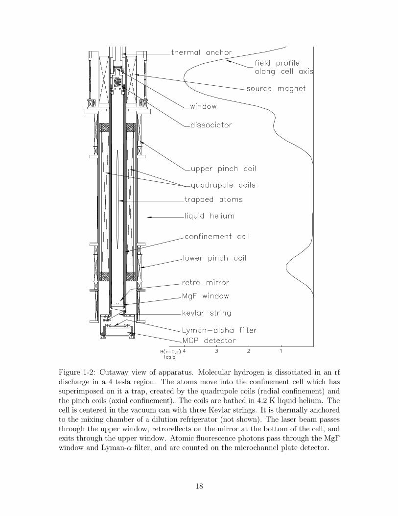
Figure 1-2: Cutaway view of apparatus. Molecular hydrogen is dissociated in an rfdischarge in a 4 tesla region. The atoms move into the confinement cell which hassuperimposed on it a trap, created by the quadrupole coils (radial confinement) andthe pinch coils (axial confinement). The coils are bathed in 4.2 K liquid helium. Thecell is centered in the vacuum can with three Kevlar strings. It is thermally anchoredto the mixing chamber of a dilution refrigerator (not shown). The laser beam passesthrough the upper window, retroreflects on the mirror at the bottom of the cell, andexits through the upper window. Atomic fluorescence photons pass through the MgFwindow and Lyman-α filter, and are counted on the microchannel plate detector.

18

away from the z axis of the trap (the potential exhibits near cylindrical symmetryabout the z axis); the potential is small and roughly uniform for about 20 cm alongthe z axis. “Pinch” coils at each end provide the axial confinement. The field profileindicated in figure 1-2 is along the z axis of the cell.

The trap depth sets an energy scale: for atoms to be trapped their total energymust be less than the trap depth. Two techniques are used to cool the atoms into thetrap. First, after H2 molecules are dissociated [17, 19] the hot atoms are thermalizedon the walls of the cell, held at 275 mK. In order to prevent the atoms from stickingtightly to the cold surfaces, a superfluid 4He film covers the walls and reduces thebinding energy of the H atoms to a manageable 1.0 K [20, 21, 22]. When the atomsleave the wall their total energy (3kBT/2 of kinetic energy and ǫt of potential energy)is still greater than the trap depth. The second stage of cooling into the trap involvescollisions among the atoms that are crossing the trapping region. Sometimes thesecollisions result in one atom having low enough energy to become trapped. Thepartner atom in the collision goes to the wall and is thermalized. The gas densitiesexpected in the cell correspond to a collision length many times greater than the celldiameter, so atoms pass through the trapping region many times before becomingtrapped. A recent study of the trap loading process will be published elsewhere [19].

After loading the trap, the cell walls are quickly cooled to below 150 mK to ther-mally disconnect the sample from the confinement cell. At these lower temperaturesthe residence time of an atom on the surface of the cell becomes much longer than thecharacteristic H+H→ H2 recombination time, and so the surface is “sticky”; all theatoms that reach the surface recombine before having a chance to leave the surface.Thermal disconnect between the cryogenic cell and the trapped sample is achievedbecause no warm particles can leave the walls and carry energy to the trapped gas.Atoms can leave the trapped gas and reach the wall, however, if they have largeenough total energy to climb the magnetic hill. As these very energetic atoms irre-versibly leave the trapped sample, it cools. In fact, this preferential removal of themost energetic atoms, called evaporation, is very useful. It is the cooling mechanismwe exploit to create samples as cold as 20 µK, as described in chapter 5. A thoroughdescription of the heating and cooling processes which set the temperature of thesystem is found in appendix A.

We catch both the d and c low field seeking states in the trap. However, inelasticcollision processes involving two c state atoms quickly deplete the c-state population,and the remaining atoms constitute a doubly polarized sample (both electron andproton spins are polarized). Because the spin state is pure, the spin-relaxation rateis rather small. For peak densities in the normal gas of n ≃ 1014 cm−3 (nearly thelargest for these experiments) the characteristic decay time is 40 s.

The trapped gas is probed using various techniques. The simplest method involvesquickly lowering the magnetic confinement barrier at one end of the trap, and mea-suring the flux of escaping atoms as a function of barrier height [17, 23]. In a limitedregime this technique can be used to infer the gas temperature and density. This tech-nique, and its limitations, is described in chapter 4. Another technique is rf ejectionspectroscopy, described in chapter 4. The third probe technique is laser spectroscopyof the 1S-2S transition, envisioned [24, 16], realized [14, 25], and perfected [13] in our

19

lab for a trapped gas. This diagnostic tool can give the density and temperature ofthe gas over a wider range of operating conditions than the other techniques, and hasproven crucial for studies of BEC. The laser probe will be described in more detail inchapter 5, and is a principle subject of the companion thesis by Killian [13].

20

Chapter 2

Theoretical Considerations

This chapter addresses two important topics from a theoretical perspective. First, weexplain why previous experiments could not bring trapped hydrogen into the quantumdegenerate regime. This understanding allowed us to solve the problem and achieveBEC. The second topic is related to the small fraction (only a few percent) of atomswe are able to put into the condensate. This situation differs markedly from thatobserved in Rb and Na BEC experiments. An explanation of this difference andothers is the second topic we explore theoretically.

The starting point for understanding the behavior of the trapped gas is classicalstatistical mechanics. Good explanations have been developed elsewhere [26, 27, 17,28]. For completeness, we present a development in appendix A. Since the gasexists in a trap of finite depth ǫt, we use a truncated Maxwell-Boltzmann occupationfunction. Knowledge of the trap shape allows us to calculate the population, totalenergy, density, etc. The effects of truncation of the energy distribution at the trapdepth are included in these derivations. We see that for deep traps (η ≡ ǫt/kBT > 7)the truncation does not significantly alter the properties of the system from estimatesbased on an untruncated distribution. Appendix A also explains the density of statesfunctions (see section A.1.2) used in the remainder of the thesis and summarizesevaporative cooling (see section A.2).

2.1 Dimensionality of Evaporation

The temperature of the gas is set by a balance between heating and cooling processes,as described in section A.2.2. Previous attempts to attain BEC in hydrogen [29, 30]failed because the cooling process became bottlenecked by the slow rate at whichenergetic atoms could escape, thus reducing the effective cooling rate. To understandthis bottleneck we must first consider the details of the trap shape. We then studythe motion of the particles that have enough energy to escape.

The trap shape used to confine samples at T < 200 µK is often called the “Ioffe-Pritchard” [31, 26] type (labeled “IP”). Using axial coordinate z and radial coordinate

21

ρ, the potential has the form

VIP (ρ, z) =√

(αρ)2 + (βz2 + θ)2 − θ (2.1)

with radial potential energy gradient α (units energy/length), axial potential energycurvature 2β (units of energy/length2), and bias potential energy θ. See section A.1.2for a summary of the density of states functions for this trap.

In the limit of ρ ≪ θ/α, the Ioffe-Pritchard potential is harmonic in the radialcoordinate, as may be seen by expanding the potential in powers of αρ/(βz2 + θ):

VIP (ρ, z) = βz2 +1

2

α2

βz2 + θρ2 +

1

8

α3

(βz2 + θ)2ρ3 + · · · . (2.2)

The trap is harmonic in the radial direction when the third term is much smallerthan the second term. This is true for radial coordinates ρ≪ ρanharm, where we havedefined the “anharmonic radius” at which the second term matches the third term:

ρanharm ≡ 4βz2 + θ

α. (2.3)

The trap appears harmonic in all three directions to short samples for which the radialoscillation frequency is essentially uniform along the length of the sample. This occursfor temperatures T ≪ 4θ/kB. In the harmonic regime, the axial oscillation frequencyis

ωz =

√

2β

m, (2.4)

and the radial oscillation frequency is

ωρ = α

√

m

βz2 + θ. (2.5)

For the evaporation to proceed efficiently, atoms with energy greater than thetrap depth ǫt (called “energetic atoms”) must leave the trap promptly, before havinga collision. As shown in appendix B, in the vast majority of cases an energetic atomthat collides with a trapped atom will become trapped again. The rare collision thatproduced the energetic atom will be “wasted”. It is essential to understand the detailsof the particle removal process if maximum evaporation efficiency is to be achieved.

Previous attempts to cool hydrogen to BEC utilized “saddlepoint evaporation”,in which energetic atoms escape over a saddlepoint in the magnetic field barrier atone end of the trap. To escape, the atom must have energy in the axial degree offreedom (z) that is greater than ǫt. This atom removal technique is inherently onedimensional. The collisions which drive evaporation produce many atoms with highenergy in the radial degrees of freedom, and in order for these to escape the energymust be transferred to the axial degree of freedom. This energy transfer process wasanalyzed theoretically by Surkov, Walraven, and Shlyapnikov [32], and we follow theiranalysis.

22

In a harmonic trap the potential is separable, and the particle motion is com-pletely regular; no energy exchange occurs. In the Ioffe-Pritchard trap, however,energy exchange can occur because the potential is not separable; the radial oscilla-tion frequency depends on the axial coordinate, z, and so radial motion can coupleto axial motion. (See equation 2.5.)

This energy mixing can be understood by considering how rapidly the radial oscil-lation frequency changes as an atom moves along the z axis. If the frequency changesslowly (“adiabatically”), then the energy will not mix among the degrees of freedom.The adiabaticity parameter is the fractional change of the radial oscillation frequencyin one oscillation period as the atom moves axially through the trap. Strong mixingoccurs when

ωρω2ρ

∼ 1. (2.6)

Here ωρ = (dωρ/dz)(dz/dt). For a Ioffe-Pritchard trap with a bias that is large

compared to kBT , ωρ = α/√

(βz2 + θ)m. We have used the expansion of VIP fromequation 2.2, which is valid if kBT ∼ αρ≪ θ. Given that kBT ≪ θ, the adiabaticityparameter is

ωρω2ρ

= vzβz

√m

α√βz2 + θ

. (2.7)

We see that several factors contribute to good mixing: large axial velocity vz (whichoccurs at high temperature), small radial gradient α, small bias field θ, and largeaxial curvature β. In practice, however, achieving BEC requires low temperatures(vz small) and high densities (obtained with large compressions, and thus large α).Consequently, the degrees of freedom do not mix and evaporation becomes essen-tially one dimensional. Typical values for our experiment are α/kB = 16 mK/cm,β/kB = 25 µK/cm2, θ/kB = 30 µK, T = 100 µK, z ∼ 2 cm, and vz = 140 cm/s, sothat ωρ/ω

2ρ ∼ 10−3. For these conditions it takes about 103 oscillations to transfer

energy, but there are only about ωρ/2πΓcol ∼ 200 oscillations per collision for a peaksample density n0 = 1014 cm−3 (Γcol is the elastic collision rate, p121). There is notenough time to transfer the radial energy to axial energy before the particle has a col-lision. The energy mixing is thus very weak and the evaporation is one dimensional.Surkov et al. [32] pointed out the consequences of one-dimensional evaporation. Theyestimated that the efficiency is reduced by a factor of 4η compared to that of full 3Devaporation. The evaporative cooling power thus drops dramatically. Experimentsin our laboratory (unpublished) have confirmed that phase space compression ceasesnear 100 µK. These results were duplicated and studied in more depth by Pinkse et

al. [30].

In order to maintain the evaporation efficiency a technique is required that quicklyremoves all particles with energy greater than the trap depth. To this end we imple-mented rf evaporation, as described in detail in chapter 3.

2.2 Degenerate Bose Gas

23

2.2.1 Bose Distribution

The statistical mechanical description of a classical gas, presented in appendix A,is not correct when quantum effects are important. A simple way to understandthe crossover to the quantum regime is to recall that particles are characterized bywavepackets whose size is related to their momentum by the Heisenberg momentum-position uncertainty relation. As a gas is cooled, the particle momenta decrease,and the wavepackets enlarge. The classical (point-particle) description of the systembreaks down when these wavepackets begin to overlap. The quantum treatment cor-rectly deals with the effect of particle indistinguishability. There are many excellenttreatments of quantum statistical mechanics [33]. Here we review the basic featuresthat are important for our experiment.

A collection of identical particles with integer (half-integer) spins must have a totalwavefunction that is symmetric (anti-symmetric) when two particles are exchanged.The connection between spin and symmetry has been explained using relativisticquantum field theory [34]. Particles with integer (half-integer) spin are called bosons(fermions). In contrast to fermions, multiple bosons may occupy a single quantumstate.

The occupation function for a gas of N identical bosons in a box of volume V , andin the limit of N → ∞ and V → ∞ but constant N/V , is called the Bose-Einsteinoccupation function [33]

fBE(ǫ) =1

exp(ǫ−µ)/kBT −1, (2.8)

where µ and T are Lagrange multipliers which constrain the system to exhibit thecorrect population and total energy through the conditions

N

V=∫

dǫρ(ǫ)

VfBE(ǫ) (2.9)

andE

V=∫

dǫ ǫρ(ǫ)

VfBE(ǫ). (2.10)

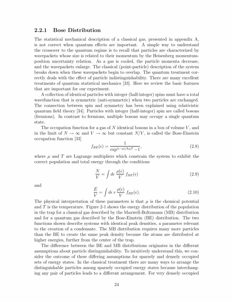
The physical interpretation of these parameters is that µ is the chemical potentialand T is the temperature. Figure 2-1 shows the energy distribution of the populationin the trap for a classical gas described by the Maxwell-Boltzmann (MB) distributionand for a quantum gas described by the Bose-Einstein (BE) distribution. The twofunctions shown describe systems with identical peak densities, a parameter relevantto the creation of a condensate. The MB distribution requires many more particlesthan the BE to create the same peak density because the atoms are distributed athigher energies, further from the center of the trap.

The difference between the BE and MB distributions originates in the differentassumptions about particle distinguishability. To intuitively understand this, we con-sider the outcome of these differing assumptions for sparsely and densely occupiedsets of energy states. In the classical treatment there are many ways to arrange thedistinguishable particles among sparsely occupied energy states because interchang-ing any pair of particles leads to a different arrangement. For very densely occupied

24

Figure 2-1: Comparison of Maxwell-Boltzmann (dashed line) and Bose-Einstein(solid line) distributions of particle energies, plotted for various chemical potentials.The peak density, a quantity related to the onset of BEC and to evaporation and decayrates, is identical for each pair of curves. The vertical axis is the number of atoms withthe given energy. This is proportional to the occupation function weighted by thetotal energy density of states for a Ioffe-Pritchard trap, ∝ ǫ3 +2θǫ2. Here θ/kBT = 1.

states, interchanges of distinguishable particles often result in the same arrangementbecause the particles often do not change energy level. For a collection of distinguish-able particles with a given total energy, there are “extra” arrangements in whichthe particles are sparsely distributed. In contrast, for indistinguishable particles anyinterchange of two particles results in the same overall arrangement of particles, re-gardless of whether the states are sparsely or densely occupied. There are thus no“extra” sparse arrangements of particles.

In a gas near the quantum degenerate regime the occupation of the energy levels

25

ranges from dense (∼ 1 at low energies) to sparse (≪ 1 at high energies). Usingthe assumption of equal a priori probabilities [33], distinguishable particles will mostlikely be found in those arrangements with the more sparse level occupations (higheroverall energies) because there are so many more of these arrangements. Indistin-guishable particles give no rise to such “extra” arrangements, and so the most likelyarrangements will involve more dense level occupations (lower overall energies) thanpredicted by classical theory. Figure 2-1 demonstrates this effect. For each pair ofcurves the peak density, n0, is identical. The peak density is the experimentally ob-servable quantity. Since the MB occupation function favors arrangements with higherenergy (and thus atoms are distributed over a larger volume in the trap), more atomsare required in the sample to produce the same peak density. The curves thus do notexhibit equal area.

Bose-Einstein condensation occurs when the chemical potential goes to zero andthe occupation of the lowest energy state diverges. This occurs at the critical density[33]

nc = g3/2(1)/Λ3(T ) (2.11)

where gn(z) ≡ ∑∞l=1 z

l/ln; g3/2(1) = 2.612. A gas that has undergone the Bose-Einstein phase transition is said to be in the quantum degenerate regime because amacroscopic fraction of the particles are in an identical quantum state.

Although a hydrogen atom consists of two fermions, it behaves like a compositeboson for the studies in this thesis because the collision interaction energies are ex-tremely small compared to the electron-proton binding energy [35]. The two fermionsact as a unit except in high energy collisions where electron exchange is possible. Thetypical interaction energy during low temperature collisions is ∼ 1 mK, which corre-sponds to 10−7 eV, 108 times smaller than the binding energy.

To analyze the behavior of the degenerate Bose gas we shall separately treat thecondensed and non-condensed portions of the system. The condensate is treatedin section 2.2.2. The non-condensed fraction, which we call the “normal gas” or“thermal gas”, is treated in appendix C. The results derived here will be used tounderstand how the hydrogen system is different from other gases that have beenBose condensed (section 2.3), and to interpret the experimental results in chapter5 (note that truncation effects are important because of the shallow traps used forthose experiments, 4 < η < 6).

2.2.2 Description of the Condensate

2.2.2.1 Gross-Pitaevskii Equation

When Bose-Einstein condensation occurs, a macroscopic fraction of the particles oc-cupy the lowest energy quantum state of the system, and thus have the same wave-function. For a non-interacting Bose gas, that wavefunction is simply the lowestharmonic oscillator wavefunction for the trap. Interactions become important whenmany particles occupy this region of space and the local density increases. In thiscase the wavefunction spreads out due to repulsion among the atoms. There is a largebody of literature on Bose-Einstein condensates (see [36] for a recent review), and so

26

we simply quote here the most important results.The Schroedinger equation for the interacting condensate is called the Gross-

Pitaevskii equation [37, 38, 39], and has the form

− h2

2m∇2ψ(r) + V (r)ψ(r) + U0 |ψ(r)|2 ψ(r) = µψ(r) (2.12)

where ψ(r) is the condensate wavefunction to be determined. The eigenenergy of thewavefunction is µ, which is the total energy of each condensate atom. The quantityU0 ≡ 4πh2a/m parameterizes the mean field energy, which is the energy of interactionamong the atoms per unit density, and is repulsive for s-wave scattering lengths a > 0.For hydrogen in the ground state, a = 0.648 A[40], and U0/kB = 3.92×10−16 µK cm3.The mean field energy augments the trap potential by an amount proportional tothe local condensate density ncond(r) = |ψ(r)|2. Note that interactions between thecondensate and non-condensed atoms are neglected here. For the experiments in thisthesis, this interaction energy is small because the density of non-condensed atoms(called the “thermal gas” or “normal gas”) is small. Furthermore, the interactionenergy with the thermal gas is essentially uniform across the condensate becausethe density of non-condensed atoms varies only weakly; the thermal energy of thenormal gas (Tc ∼ 60 µK) is much larger than the condensate mean field energy(µ/kB ∼ 2 µK), and thus the density of the normal gas does not change appreciablyon the length scale of the condensate.

We identify the eigenenergy µ in equation 2.12 with the chemical potential of thesystem in equilibrium. The chemical potential is the energy required to add a particleto the system. When a condensate is present, the normal gas is “saturated”, and anyparticles added to the system go into the condensate. The energy required to add thelast atom to the condensate is µ, the eigenenergy, and so we link µ with the chemicalpotential. In practice we measure µ spectroscopically through the peak density atthe center of the condensate, which is in turn measured through the cold-collisionfrequency shift. This is explained in section 5.3.1.

2.2.2.2 Thomas-Fermi Approximation

If the condensate density is large enough so that the mean field energy is much greaterthan the kinetic energy of the wavefunction, then the kinetic energy term (also calledthe quantum pressure term) in equation 2.12 may be neglected. Using this “Thomas-Fermi” approximation we obtain the condensate density profile

ncond(r) = np − V (r)/U0 (2.13)

where np ≡ µ/U0 is the peak condensate density (the largest density in the condensate,found at the bottom of the trap). The Thomas-Fermi approximation is valid overmost of the volume of the condensate, but near the edges the condensate densityapproaches zero, and the kinetic energy term should be included. We ignore thissmall correction in the calculations which follow because it is minor for interpretationof the experiments described in this thesis. See [41] for a good description of various

27

ways to go beyond the Thomas-Fermi approximation.The condensate density profile may be obtained without the Gross-Pitaevskii

equation by assuming the condensate is stationary and its particles are at rest, andthen balancing hydrodynamic forces [42]. A condensate particle in a region of poten-tial energy ε has total energy E = ε + ncond(ε)U0. Since there must be no net forceon the particle, E = const ≡ npU0 and ncond(ε) = np − ε/U0.

2.2.2.3 Population and Loss Rate

The population of the condensate is easily computed using the Thomas-Fermi wave-function in the bottom of the IP trap, which is parabolic for the condensate sizesand trap parameters of interest in this thesis. We approximate the potential energydensity of states (see p114) as (ε) ≈ AIP

√εθ and obtain

Nc =∫ U0np

0dε AIP θ

√ε(np − ε/U0)

=4

15AIP θ U

3/20 n5/2

p . (2.14)

As noted above, the total energy of each condensate atom is the chemical potentialµ = npU0, so Ec = µNc.

The loss rate from the condensate due to two-body dipolar relaxation is found byintegrating the square of the density over the volume of the condensate:

N2,c = −∫ U0np

0dε AIP θ

√ε (g/2!) (np − ε/U0)

2

= − 16

105

g

2!AIPθ U

3/20 n7/2

p (2.15)

where the 2! accounts for correlation properties of the condensate [43, 44]. Here thedipolar decay rate constant g is slightly different from that given in equation A.19because the rate constant Gdd→cd should be multiplied by 2; the energy θ liberatedin this process is large compared to µ. This term is small, so g is not effected much.The energy loss rate is E2,c = µN2,c. The characteristic condensate decay rate in aparabolic trap is

− N2,c

Nc=

2

7gnp, (2.16)

which is 1.6 s−1 for a typical peak density np = 5 × 1015 cm−3.

2.3 Properties of a Bose-Condensed Gas of Hydro-

gen

Hydrogen differs in several ways from alkali metal atoms that have been Bose con-densed. The principal differences are its small mass and small s-wave scatteringlength. How do these properties influence the system?

28

First, the small mass implies that BEC occurs at a higher temperature for a givenpeak density: from equation 2.11, Tc ∝ 1/m. We have observed the transition attemperatures roughly 50 times higher than in the other systems.

Further, as estimated by Hijmans et al. [45] and will be shown in the followingsections, the maximum equilibrium condensate fraction is small for hydrogen. Thiswill be explained by noting the relatively high density of the condensate, as comparedto the thermal cloud. This high density leads to high losses through dipolar decay,which result in heating of the system. This heating must be balanced by evaporativecooling, which proceeds slowly in hydrogen because of the small collision cross section.The result of these factors is that only small condensate fractions are possible inequilibrium. Possible remedies will be noted.

Finally, hydrogen’s small collision cross-section should allow condensates of H tobe produced by evaporative cooling that contain many orders of magnitude moreatoms than those possible in alkali-metal species, as explained in the section 2.3.4.

2.3.1 Relative Condensate Density

For trapped hydrogen, the condensate density grows much greater than the densityof the non-condensed portion of the gas at even very small condensate fractions [18],a distinct difference from other species that have been Bose-condensed. This is note-worthy for possible future studies of behavior near the phase transition. As shown insection 2.3.2, it also has implications for the maximum condensate fraction that maybe achieved in hydrogen. In this section we calculate the ratio of the densities as afunction of the condensate fraction. We compare hydrogen to Li, Na, and Rb.

The condensate fraction is

F ≡ Nc

Nc +Nt(2.17)

where the population of the thermal cloud, Nt, is found using equation C.7 and thepopulation of the condensate is given by equation 2.14. The fraction can be writtenin terms of the more convenient population ratio, f ≡ Nc/Nt, as F = f/(1 + f). Fora given peak condensate density, sample temperature, and set of trap parameters, thepopulation ratio is

f =

(

27/2h6a3/2

π7/2m3kB3

)

︸ ︷︷ ︸

f0

(

φ

π4 + 60ζ(3)φ

)

︸ ︷︷ ︸

ftrap(φ)

(

n5/2p

T 3c A0(η, φ)

)

︸ ︷︷ ︸

fsample

(2.18)

where f0 = 7.37 × 10−34 (cm3)5/2µK3 for H; ftrap indicates whether the trap shapeexperienced by the thermal cloud is predominantly harmonic (large φ) or predomi-nantly linear (small φ) in the radial direction (φ ≡ θ/kBT is a unitless measure of thetrap bias energy); and fsample carries the details of the thermal cloud and condensateoccupation.

The ratio of the peak condensate density to the critical BEC density, R ≡

29

species m a Tc Ratom φ ftrap(φ) R0Ratom/ftrap(φ)2/5

H 1 0.648 [40] 60 230 0.6 0.0043 94Li [5] 7 -14.4 [46] 0.30 98 2.2 × 105 0.012 25

Na [47] 23 27.5 [48] 2.0 26 30 0.013 6.8Rb [44] 87 57.1 [49] 0.67 16 160 0.011 4.4

Table 2.1: Comparison of the parameters governing the ratio of condensate densityto thermal gas density for the various BEC experiments. The units are amu, A, µK.The density ratio (for small condensate fractions) is the last column multiplied by thecondensate fraction to the 2/5 power. This ratio is much larger for H than for Na orRb, indicating that two-body loss from the condensate becomes important at muchlower f . For Li, hydrodynamic collapse of the condensate occurs before the two-bodyloss process studied here becomes important.

np/nc(Tc), can be expressed in terms of the occupation ratio as

R =

(

1

229/10g3/2(1)π1/10

)

︸ ︷︷ ︸

R0

(

h2

mkBTca2

)3/10

︸ ︷︷ ︸

Ratom

(

fA0(η, φ)

ftrap(φ)

)2/5

(2.19)

The prefactor is R0 = 0.0457364. Table 2.1 gives the parameters appearing in equa-tion 2.19 for the various BEC experiments. For even a small occupation ratio off = 0.05, the H condensate will be 28 times more dense than the thermal gas, whichcan be compared to a Rb condensate that will be only be 1.3 times more dense. Theloss rates from the condensate are thus very different for the two systems, as shownin the next section. Note that the trap oscillation frequencies play no role in these re-sults. The only assumptions are that the trap is of the IP form with bias field1 φ, thatthe condensate is in the Thomas-Fermi regime, and that µ≪ kBT so that mean-fieldinteraction energy of the condensate with the thermal cloud can be neglected.

2.3.2 Achievable Condensate Fractions

The temperature of a trapped sample, and thus its condensate fraction, is set by acompetition between heating and cooling, as described in section A.2.1. Hydrogen’sanomalously low scattering length means that the elastic collision rate is small, andthus evaporation proceeds slowly. The evaporative cooling power is small, and theheating-cooling balance favors higher temperatures and lower condensate fractionsthan would occur if hydrogen had a larger collision cross section. Higher temperaturesare also favored by the large density of the condensate, which places an extra heatload on the system due to dipolar relaxation. This extra heat load can easily be muchlarger than the dipolar relaxation heat load of the thermal gas. In this section we

1When φ is small, the condensate experiences a harmonic potential while the thermal gas expe-riences a predominantly linear potential in the radial direction. When φ is large, both condensateand thermal gas experience the same potential functional form.

30

N

N evap

.

2,c

.

loss

thermalcloud

condensate

2,tN .

condensate

gain

evaporation:

dipolar

decay:

system boundary

Figure 2-2: Diagram of system consisting of thermal cloud and condensate. Weassume the particle and energy exchange rates between the condensate and thermalcloud are fast compared to the loss rates. The dynamics of the gas are set by evap-oration and dipolar decay from the normal gas when the condensate is small. Whenthe condensate is large, however, N2,c ≫ N2,t, and the dynamics are dominated bythe dipolar decay rate from the condensate in balance with the evaporation rate.

examine each of these factors in more detail.

We model the system as two components, the condensate and thermal gas, thatare strongly linked. As indicated in figure 2-2, losses from the system occur throughdipolar decay in the thermal gas, dipolar decay in the condensate, and evaporationfrom the thermal cloud. We assume that particles and energy are exchanged betweenthe condensate and thermal gas quickly compared to all loss rates. The system is ina dynamic equilibrium. In section 2.3.3 we examine the validity of the assumption offast feeding of the condensate.

2.3.2.1 Dipolar Heating Rate

Here we study the rate of heating the system due to dipolar decay in the condensateand in the thermal gas. We define heating as the removal of atoms from the samplewhich carry less than the average amount of energy per particle. We find that forhydrogen the condensate heat load exceeds the thermal gas heat load at condensatefractions of 0.3%. We then compare this ratio for H to that of the atomic species inother BEC experiments. While illustrative, this comparison is not completely appro-priate because the loss mechanisms in the other systems are different. Hydrodynamiccollapse of the Li condensate prevents it from growing larger than about 1000 atomsin the experiments of Hulet et al. [5, 50]. Three-body loss process are dominant overtwo-body dipolar decay in the Rb and Na experiments. The comparison made in this

31

section therefore serves simply to indicate how different hydrogen is from the otherspecies.

The heating rate for a process (labeled σ), with energy and particle loss rates Eσand Nσ, is the difference between the average energy per particle in the system andthe energy per particle that is removed, multiplied by the rate at which particles areremoved:

Hσ = Nσ

(

Eσ

Nσ

− E

N

)

(2.20)

where E/N is the average energy per particle for the whole system. In this analysisN = Nc +Nt. The characteristic rate for this process is Hσ/E.

We wish to find the ratio of the heating rates due to dipolar decay from thecondensate (Hc) and from the thermal cloud (Ht) as a function of the occupationfraction f . Losses from the condensate play a significant role in the trap dynamicswhen Hc ≥ Ht.

By inverting equation 2.14 to get np, and using the definition of f , we obtain N2,c

(from equation 2.15) in terms of f and Nt. For a small condensate (i.e. µ ≪ Et),straightforward algebra obtains

Hc

Ht= f 7/5

(

h2

mkBTca2

)3/10

︸ ︷︷ ︸

Ratom

π2/5

221/10 105

(π4 + 60ζ(3)φ)7/5A0(η, φ)7/5

φ2/5Q1(φ, η)(

1 − Q2(φ,η)A0(η,φ)(1+f)Q1(φ,η)A1(η,φ)B(φ)

)

︸ ︷︷ ︸

C(φ, η, f)

(2.21)

where B(φ) was defined in equation C.12. The function C(φ, η, f) has only weakdependence on f for f ≪ 1, so the dominant dependence of the heating ratio on theoccupation fraction is f 7/5. The function C(φ, η, f = 0) is plotted in figure 2-3.

For the experiments described in this thesis φ ∼ 0.6 and η ∼ 5. Then C ∼ 17,and for small f

Hc

Ht= f 7/5 3.9 × 103. (2.22)

The heating rates are equal when f = 0.27%. This means that heating of the sampledue to losses from the condensate becomes a very significant problem even whenthe condensate is still quite small. It is difficult to hold the system in equilibriumfor large condensates because the heat load that must be balanced by evaporationquickly grows too large. To obtain a large condensate fraction, the normal gas could,of course, be removed, and then E/N would be µ. The heating rate would be zero.However, the condensate would decay quickly and there would be no reservoir fromwhich to replenish it.

The experiments on hydrogen may be compared to other BEC experiments usingNa, Rb, and Li. Relevant values for the quantities in equation 2.21 are tabulated intable 2.2. These values help us understand why high equilibrium condensate fractionscan be created in Na and Rb systems. Note that three-body loss processes, whileinsignificant in hydrogen, are the limiting factor which precludes larger condensatedensities in Na and Rb.

32

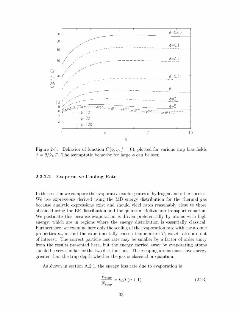
Figure 2-3: Behavior of function C(φ, η, f = 0), plotted for various trap bias fieldsφ = θ/kBT . The asymptotic behavior for large φ can be seen.

2.3.2.2 Evaporative Cooling Rate

In this section we compare the evaporative cooling rates of hydrogen and other species.We use expressions derived using the MB energy distribution for the thermal gasbecause analytic expressions exist and should yield rates reasonably close to thoseobtained using the BE distribution and the quantum Boltzmann transport equation.We postulate this because evaporation is driven preferentially by atoms with highenergy, which are in regions where the energy distribution is essentially classical.Furthermore, we examine here only the scaling of the evaporation rate with the atomicproperties m, a, and the experimentally chosen temperature T ; exact rates are notof interest. The correct particle loss rate may be smaller by a factor of order unityfrom the results presented here, but the energy carried away by evaporating atomsshould be very similar for the two distributions. The escaping atoms must have energygreater than the trap depth whether the gas is classical or quantum.

As shown in section A.2.1, the energy loss rate due to evaporation is

Eevap

Nevap

≃ kBT (η + 1) (2.23)

33

species ma2T 2c C(φ, η = ∞, f = 0) f=

H 1000 16 0.28 %Li [5] 130 7.2 0.91 %

Na [47] 70,000 7.4 2.3 %Rb [44] 130,000 8.3 3.1 %

Table 2.2: Comparison of the parameters entering the heating/cooling balance forthe various BEC experiments. The units are amu, A, µK. The second column,ma2T 2

c , is proportional to the cooling rate. The third column carries the trap shapedependence of the dipolar decay process in the thermal gas. The forth column,f= = (RatomC(φ,∞, 0))−5/7, is the occupation fraction at which the heating rate dueto dipolar decay in the thermal cloud matches that due to the condensate.

for η > 6. The cooling rate is

Hevap = Nevap

(

Eevap

Nevap

− E

N

)

(2.24)

which, for large η, is NevapkBT times a factor which depends linearly on η. Tocompare the cooling rates of gases of different species, it is thus sufficient to considerNevap/N ∼ n0σve

−η(η + const). When n0 = nc(Tc), the ratio is, for fixed η,

Nevap

N∝ (mkBTc)

3/2

h38πa2

√

8kBTcπm

∝ ma2T 2c (2.25)

which is listed in table 2.2. We see that, for a similar η, the cooling rate for H is muchsmaller than that for Na and Rb. To increase the cooling rate in H, the parameter ηmust be reduced, which reduces the cooling efficiency.

We conclude that the equilibrium condensate fraction expected in H is muchsmaller than that in Na and Rb for two reasons. First, loss from the condensatesignificantly influences the thermodynamics of the system at much lower condensatefractions in H experiments since f= is so small. Furthermore, the cooling rate for agiven η is much less in the H experiment. It is thus easier to achieve large condensatefractions in Rb and Na than in H. Note that the condensate fraction for Li experimentsis limited by hydrodynamic collapse of the condensate [50].

A possible remedy for the low evaporation rate in H experiments has been sug-gested by Kleppner et al. [51]. A small admixture of impurity atoms in the trap couldact as “collision moderators” since the collision cross section with H would most likelynot be anomalously low; it should be on the order of 103 times larger than that of H-Hcollisions. The increased evaporation rate should allow more atoms to be condensed,and with a much faster experimental cycle time.

34

2.3.3 Condensate Feeding Rate

As the condensate decays by dipolar relaxation it must be fed from the thermal cloud(which is assumed to be at the critical BEC density, nc). This feeding process maybe bottlenecked by the small collision cross section, σ, of hydrogen. To estimatethe maximum condensate replenishment rate, Rmax, we consider the event rate forcollisions between two thermal atoms assuming that the collisions occur inside thecondensate. Ignoring stimulated scattering for the moment, this rate is the collisionrate per atom times the number of thermal atoms in the region of the condensate,

Ncol,feed = (ncσvBE√

2) (Vcond nc) (2.26)

where

vBE =g2(e

µ/kBT )

g3/2(eµ/kBT )

√

8kBT/πm (2.27)

is the mean particle speed in a Bose gas (ignoring truncation; g2(1)/g3/2(1) = 0.6297).The condensate volume (for samples in the Thomas-Fermi regime) is, using equation2.13,

Vcond = 2AIP µ3/2

µ

5+θ

3

. (2.28)

For small chemical potentials we approximate Vcond = 2AIPθµ3/2/3. We assume that

some fraction ζ of the collisions result in an atom being added to the condensate.One might expect ζ to be less than unity because only a fraction of collisions involveatoms with initial momentum and energy consistent with one atom going into theBEC wavefunction, which has nearly zero momentum and energy. On the otherhand, the Bose enhancement factor very strongly favors population of the condensate.Calculations by Jaksch et al.[52] (equation 19a) indicate that for a condensate nearits equilibrium population, and with µ ≪ kBT , the fraction is ζ ∼ 1/5. For themoment we leave the parameter free. The maximum condensate replenishment rateis ζNcol,feed.

In equilibrium the condensate population is varying slowly compared to the feedingand loss rates. We may therefore equate the maximum replenishment rate to thecondensate dipolar decay loss rate (from equation 2.15):

− N2,c = ζNcol,feed

16

105

g

2!AIPθ U

3/20 n7/2

p =2√

2

3ζn2

cσvBEAIPU3/20 n3/2

p (2.29)

We find that the loss rate matches the maximum feeding rate when the ratio of peakcondensate density to thermal density is

npnc

= a

√

280ζ

g√π

(

kBT

m

)1/4

. (2.30)

For hydrogen at T = 60 µK and ζ = 1 the ratio is np/nc = 16. The ratio is strongly

35

influenced by the scattering length, and is about 30 times larger for the Rb experimentlisted in table 2.2, assuming a decay rate g = 10−16 cm3/s [44]. In the experimentsdescribed in chapter 5 the largest observed value of this ratio is about 20.

A detailed understanding of the maximum condensate feeding rate is clearly de-sirable, but is beyond the scope of this thesis. Nevertheless, it is clear that the finiterate of replenishing the condensate from the thermal cloud can bottleneck growth ofthe condensate.

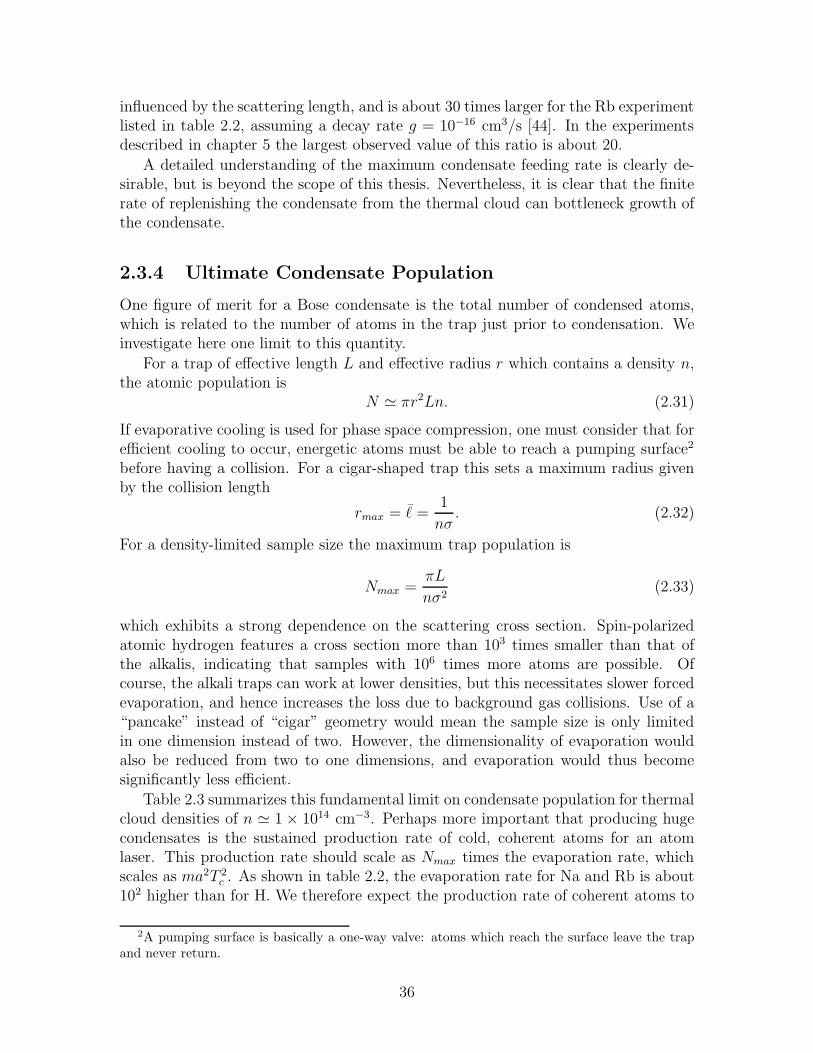
2.3.4 Ultimate Condensate Population

One figure of merit for a Bose condensate is the total number of condensed atoms,which is related to the number of atoms in the trap just prior to condensation. Weinvestigate here one limit to this quantity.

For a trap of effective length L and effective radius r which contains a density n,the atomic population is

N ≃ πr2Ln. (2.31)

If evaporative cooling is used for phase space compression, one must consider that forefficient cooling to occur, energetic atoms must be able to reach a pumping surface2

before having a collision. For a cigar-shaped trap this sets a maximum radius givenby the collision length

rmax = ℓ =1

nσ. (2.32)

For a density-limited sample size the maximum trap population is

Nmax =πL

nσ2(2.33)

which exhibits a strong dependence on the scattering cross section. Spin-polarizedatomic hydrogen features a cross section more than 103 times smaller than that ofthe alkalis, indicating that samples with 106 times more atoms are possible. Ofcourse, the alkali traps can work at lower densities, but this necessitates slower forcedevaporation, and hence increases the loss due to background gas collisions. Use of a“pancake” instead of “cigar” geometry would mean the sample size is only limitedin one dimension instead of two. However, the dimensionality of evaporation wouldalso be reduced from two to one dimensions, and evaporation would thus becomesignificantly less efficient.

Table 2.3 summarizes this fundamental limit on condensate population for thermalcloud densities of n ≃ 1 × 1014 cm−3. Perhaps more important that producing hugecondensates is the sustained production rate of cold, coherent atoms for an atomlaser. This production rate should scale as Nmax times the evaporation rate, whichscales as ma2T 2

c . As shown in table 2.2, the evaporation rate for Na and Rb is about102 higher than for H. We therefore expect the production rate of coherent atoms to

2A pumping surface is basically a one-way valve: atoms which reach the surface leave the trapand never return.

36

species σ rmax Nmax/Lcm2 cm cm−1

H 1.1 × 10−15 10 3 × 1016

Na 2 × 10−12 5 × 10−3 9 × 109

Rb 8 × 10−12 1.2 × 10−3 5 × 108

Table 2.3: Limits on number of trapped atoms when evaporative cooling is the solecooling mechanism. We assume a peak density n0 ≃ 1 × 1014 cm−3.

be 106−2 = 104 times bigger for H than for Na and Rb.

37

38

Chapter 3

Implementing RF Evaporation

Previous attempts to realize BEC in hydrogen were thwarted by inefficient evapora-tion (see section 2.1). This chapter discusses the solution to this problem and thehardware required to implement this solution.

In the improved apparatus an rf magnetic field couples the Zeeman sublevel of thetrapped atoms to an untrapped level, but only in a thin shell around the trap calledthe resonance region. Resonance occurs where the energy of the rf photons, hωrf ,matches the energy splitting between hyperfine states, proportional to the strengthof the trapping field. Only those atoms with enough energy to reach the high potentialenergy of the resonance region are ejected. The resonance region thus constitutes a“surface of death” which surrounds the sample, and so atoms with high energy in anydirection are able to quickly escape.

The rf evaporation scheme needed to be incorporated into an existing cryogenicexperiment. The basic geometry of the trapping cell is constrained by the supercon-ducting magnets which create the trap potential. A vertical bore of 5 cm diameter isavailable for the cell along the cylindrical symmetry axis of the magnets, as shown infigure 1-2. Into this bore fits the H2 dissociator and the plastic tube which containsthe gas as it is being trapped. The length of the trapping region is about 60 cm.The cell is thermally and mechanically anchored to the dissociator, which is anchoredto the mixing chamber of an Oxford Model 2000 dilution refrigerator. The mixingchamber is situated above the magnets.

A complete redesign of the cryogenic trapping cell was required in order to incor-porate the rf magnetic field. Any good electrical conductors in the vicinity of the rffields and thermally connected to the cell would absorb power from the rf field viarf eddy currents, causing the cell to heat up. Metals, some of which had suppliedthermal conductivity, thus needed to be eliminated. A superfluid helium jacket wasemployed to provide the heat transport formerly supplied by these metals. In addi-tion, the coils which drive the field were compensated so that the field is very weakfar away from the atoms, where the large pieces of copper that comprise the disso-ciator and mixing chamber are located. In this chapter we discuss these and otherdesign considerations, provide construction notes, and describe performance tests ofthe apparatus.

39

3.1 Magnetic Hyperfine Resonance

In this section we determine the magnitude and frequency of the rf magnetic fieldrequired to drive the evaporation efficiently. We summarize the ground states ofhydrogen, beginning with the hyperfine interaction, and then adding the Zeemaneffect. We obtain the four ground states and their energies. We then derive thematrix elements for rf transitions between these states. After making a series ofsimplifying approximations, we obtain the Rabi frequency for these transitions. Ananalytic theory for transition probabilities in N -level systems is then adapted to oursituation. We then calculate the field strength required to drive evaporation efficientlyfor the trap and sample parameters of immediate interest in this experiment.

3.1.1 H in a Static Magnetic Field

The ground states of hydrogen in a magnetic field are influenced by the hyperfineinteraction (interaction between electron and proton magnetic moments) and theZeeman interaction (the proton and electron magnetic moments interacting with theapplied magnetic field). Here we summarize Cohen-Tannoudji et al. [53] (we use SIunits).

We start in the zero magnetic field regime. The hyperfine interaction Hamiltonianis

Hhf = AI · S (3.1)

where I is the nuclear spin operator, S is the electron spin operator, andAh = 2π×νhf .The hydrogen ground state hyperfine frequency is νhf = 1.420 GHz. The total angularmomentum is F = I + S. The eigenstates |F,mF 〉 can be written in the |mS, mI〉basis:

|1, 1〉 = |+,+〉 (3.2)

|1, 0〉 =1√2

(|+,−〉 + |−,+〉) (3.3)

|1,−1〉 = |−,−〉 (3.4)

|0, 0〉 =1√2

(|−,+〉 − |+,−〉) . (3.5)

In an applied magnetic field, B = B0z, the Hamiltonian includes the Zeemanterm,

HZ = −B · (MS + MI), (3.6)

where MS = (qge/2me)S, MI = (−qgp/2mp)I, q is the electron charge (q < 0), ge ≃2.0023 is the electron gyromagnetic ratio, and gp ≃ 5.585 is the proton gyromagneticratio. The eigenstates of the combined Hamiltonian H = Hhf + HZ are then

|d〉 = |1, 1〉 (3.7)

|c〉 = cos θ |1, 0〉 + sin θ |0, 0〉 (3.8)

|b〉 = |1,−1〉 (3.9)

40

Figure 3-1: Zeeman diagram of hydrogen F = 1 states in low fields. State d istrapped, state c is untrapped, and state b is “antitrapped”, expelled from the trappingregion. At high fields the c state is trapped, as shown in figure 1-1.

|a〉 = sin θ |1, 0〉 − cos θ |0, 0〉 (3.10)

tan θ =−1 +

√1 + x2

x(3.11)

where x = −B0/Bhf , Bhf = Ah2/µBge(1+ϕ) = 506.65 G, µB = |q|h/2me is the Bohrmagneton, and ϕ = gpme/gemp ≃ 1.5× 10−3 is a measure of the relative contributionof the proton spin to the energy. The energies are, in order of decreasing energy,

Ed = µBB0(1 − ϕ) (3.12)

Ec = −Ah2

2

(

1 −√

1 + x2)

(3.13)

Eb = −µBB0(1 − ϕ) (3.14)

Ea = −Ah2

2

(

1 +√

1 + x2)

(3.15)

Figure 3-1 shows these energy levels. Confining our attention to the the low fieldswhich are of interest for trapped samples near the BEC transition and to the F = 1manifold, we see that atoms in the d state are trapped, those in the c state areuntrapped, and those in the b state are antitrapped (expelled).

41

3.1.2 H in an RF Magnetic Field

Atoms may leave the trap when their state is switched from d to a, c, or b. We drivetransitions between Zeeman sublevels by applying an rf magnetic field perpendicularto the static field1, Brf = B1x cosωrf t which couples states d and b to states c and a.Transitions between the states are induced by the interaction Hrf = −Brf ·(MS+MI)with matrix elements Hα,β cosωrf t ≡ 〈α|Hrf |β〉. The non-vanishing terms are

Hd,c

√2/µBB1 = (1 − ϕ) cos θ + (1 + ϕ) sin θ (3.16)

Hd,a

√2/µBB1 = (1 − ϕ) sin θ − (1 + ϕ) cos θ (3.17)

Hb,c

√2/µBB1 = (1 − ϕ) cos θ − (1 + ϕ) sin θ (3.18)

Hb,a

√2/µBB1 = (1 + ϕ) cos θ + (1 − ϕ) sin θ. (3.19)

In the limit of low trapping field B0, θ ≃ −B0/Bhf . We make the approximationscos θ = 1, sin θ = 0, and ϕ = 0, obtaining

Hd,c = Hb,c = hΩR (3.20)

where ΩR = µBB1/h√

2 is the Rabi frequency. We ignore the a-state since it is farseparated in energy from the F = 1 manifold. With these approximations we havean effective three level system with equal energy separation µBB0.

As the atoms move through the varying magnetic field, resonant transitions occurin a region of thickness ∆r = hΩR/α which is given by the resonance’s energy width,hΩR, scaled by the local potential energy gradient, α. In the vicinity of the resonanceregion, the Zeeman sub-levels can be assumed to vary linearly in space. For an atomwhose speed v changes only slightly as it crosses the resonance region, the energylevels may then be considered to vary linearly in time. The probability of changingZeeman sub-levels as the atom crosses the resonance region is calculated using avariant of the Landau-Zener formalism [54] for avoided level crossings. Vitanov andSuominen [55] have analytically calculated the dynamics for avoided level crossingsin systems with an arbitrary number of levels. They show that, for an atom initiallyin the d state, the probability of emerging from the resonance region in the d, c, or bstate is

Pd = (1 − p)2 (3.21)

Pc = 2(1 − p)p (3.22)

Pb = p2 (3.23)

where p = 1 − exp(−ζ) is the Landau-Zener transition probability for a two-statesystem, and

ζ = 2πhΩ2R/αv (3.24)

is the adiabaticity parameter for a particle of speed v in a magnetic field with mag-

1We consider the polarization of the rf field in more detail below

42

netic field gradient α/µB. For large ζ the atom absorbs two rf photons while in theresonance region, and emerges in the b state, antitrapped. For small ζ (the diabaticcase of interest here) there is only a small probability of leaving the trapped d state,and the vast majority of atoms that do leave this state will emerge in the c state,untrapped. They are pulled by gravity out of the trapping region along the trap axis.

3.1.3 RF Field Amplitude Requirement

In order to realize the improved evaporation efficiency we seek, the characteristic timerequired to eject an energetic atom must be less than the characteristic collision timeof these atoms [56]. This condition sets a minimum rf field amplitude.

Here we consider an atom traversing the trap radially, passing through the center.Atoms in different trajectories will be effected differently by the rf field and sampledensity. However, in order to have a significantly different orbit (while still havingenough radial energy to reach the resonance region), the atom would need high energyin both the radial and azimuthal degrees of freedom. Since this is rare (see appendixB), we ignore these orbits and focus on the simple case of purely radial motion.

The characteristic time to eject an energetic atom, τeject, is the oscillation period Tdivided by the probability of ejecting the atom per period, 4Pc. (We ignore coherencebetween resonance crossings). The atom encounters a resonance region four times perperiod since there is a resonance region on both sides of the trap, and the atom passesthrough each region twice per oscillation (assuming the turning point is outside thesurface of death). The oscillation period of a particle of mass m moving in a linearpotential with gradient α and with an initial energy ǫt is T = 4

√2mǫt/α. For the

parameters of interest (ǫt/kB ∼ 500 µK, α/kB ∼ 16 mK/cm used near the BECtransition), we obtain a period T ∼ 1 msec. Thus τeject ∼ 1 msec/4Pc.

To find Pc and the minimum rf field strength, we require that the ejection time beless than the characteristic collision time τcol = 1/n0σv (A rigorous analysis includesan average of the quantity n(ρ)v(ρ) over the atom’s trajectory, which produces acorrection factor of about 3). For atomic hydrogen near the onset of BEC at Tc ∼50 µK, τcol ∼ 100 msec. The particles thus sample the resonance region roughly400 times before having a collision. The ejection probability Pc must be at leastPmin = T/4τcol ≃ 1/400. The minimum adiabaticity parameter is then ζmin ≃ 10−3.For the gradient α and typical average velocity v ≃ 100 cm/s, we obtain a minimum

Rabi frequency Ωmin =√

αvζmin/h = 2π × 1 kHz. The minimum rf field is B1,min =

hΩmin

√2/µB = 1 mG. The thickness of the resonance region is ∆r = 30 nm, so

the approximation of a linearly varying trapping field made above is valid. We notethat for atoms with more complicated hyperfine structure (F > 1) the rf field mustbe larger because an initially trapped atom must be taken through one or moreintermediate states before arriving at an untrapped state. For a given g-factor and

hyperfine state the required Rabi frequency and rf field scale as√

ma2T 3c independent

of trap parameters (for linear and harmonic traps).

A potential problem is trap loss and heating through dipolar decay as atoms inthe c state pass through the cloud of trapped d atoms [56]. This turns out to not be

43

-12.0 -8.0 -4.0 0.0 4.0 8.0

0.00

0.04

0.08

0.12

z (cm)

rho

(cm

)

Figure 3-2: Static magnetic field which confines the gas, viewed in a plane whichcuts through the center of the trap. The vertical axis of the figure is the distanceaway from the central axis (symmetry axis) of the trap, in cm. The horizontal axis isthe long axis of the trap. The atoms are confined to the bottom of the trap near ρ = 0and z = 0. The contours are spaced by 100 µK. The arrows indicate the direction ofthe field. Note that the axes are very different lengths. This trap is used to confinesamples below T = 130 µK. In order to eject energetic atoms, the rf magnetic fieldmust be perpendicular to this trapping field. The saddlepoint in the trapping field ison the left. The top of the cell and dissociator are to the right.

a problem for trapped H. The time constant for this process is τdip = 1/Gcdnc whereGcd is the total event rate constant for dipolar decay in collisions between c and datoms. For H, the total event rate constant is Gcd ≃ 10−15 cm3/s which is about thesame as Gdd, the total event rate constant for dipolar decay through d-d collisions[57]. The density of c atoms is much less than n0 since they are free to fall out of thetrap (τfall ∼ 100 msec). We conclude that τdip is long compared to the lifetime of thesample as set by d-d dipolar relaxation. Therefore, we need not be concerned withdipolar relaxation events between the c and d atoms.

3.1.4 RF Coil Design

Here we describe the coil design considerations for creating an rf magnetic field thatwill drive evaporation efficiently in the cryogenic apparatus.

The rf magnetic field must have a component in a direction perpendicular to thetrapping field, as discussed above. Figure 3-2 indicates the direction of the trappingfield in a plane that cuts through the trap. This field is for a typical trap used forrf evaporation experiments. Along the sides of the trap the rf field must point inthe z direction. This field is generated by coils wrapped around the the cylindricalconfinement cell. These coils are termed the “axial coils”.

It is important that the rf field be weak enough at the top of the cell to avoid

44

Figure 3-3: Winding pattern of axial rf coil, shown wrapped on a section of the cellinner G-10 tube (3.8 cm OD). The coil is fed by the two wires extending out the topof the section. The loops are wound as close together as possible, and the feed wiresare laid tightly next to each other. The point z = 0 is very near the laser beam focus,and also the minimum of the trapping potential.

heating the large copper pieces which make up the cell top, discharge and mixingchamber (heating rates are outlined in section 3.2.1). The field generated by a loopof diameter a decays as (a/z)3 at large distances from the loop along the loop axis.However, the field can be made to decay as (a/z)5 if the loop is compensated ap-propriately. In the far-field the arrangement appears as a quadrupole instead of adipole. The heating rate is proportional to the squared magnitude of the field, so theheating rate falls as (a/z)10 for a compensated loop. The geometry of the axial coilswas chosen to provide large fields over the length of the cold samples and to producefields which decay rapidly outside the trapping region. The coils are wrapped aroundthe outside of the inner tube of the cell (3.8 cm diameter). They consist of three loopsin the “forward” direction at z = ±4 cm, 1 loop “backward” at z = ±3 cm, and twoloops “backward” at z = ±1.2 cm. The winding pattern is shown in figure 3-3.

Figure 3-4 shows a calculation2 of the magnitude of the rf field generated by theaxial coils along the trap axis. Figure 3-5 shows how the field decays along the trapaxis. The nearest big pieces of metal that must be kept cold are at z = 40 cm.Because the rf field is compensated well, the dominant heating of the top of the cell,dissociator, and mixing chamber arises from other mechanisms, described in section

2Since the wavelength of this radiation (λ = 3 m at 100 MHz) is much larger than the lengthscale of interest we disregard propagation effects and calculate the dc field.

45

Figure 3-4: Profiles of the rf and dc magnetic fields along the axis of the trap. Thedashed line is the rf field magnitude, and the solid line is the trapping field for thetrap used to achieve BEC.

3.4.4.

The rf fields are primarily used to remove the most energetic atoms, but it isalso sometimes desirable to remove the atoms at the very bottom of the trap wherethe trapping field is aligned along the z axis. Another set of rf coils, called the“transverse coils”, generate a field predominantly perpendicular to z. The windingpattern is shown in figure 3-6.

3.2 Mechanical Design of the Cell

The designs of the cells used previously in the experiment are described by Doyle [17]and Sandberg [16]. The principle difference between those cells and the cell used forthis experiment is the presence of the rf magnetic fields. Previous designs relied onmetals to provide thermal conductance along the length of the cell, but metals mustbe excluded in the new design. They would allow rf eddy currents to flow, whichwould heat the cell and which would screen the atoms from the applied rf fields. Insection 3.2.1 we examine the problem of rf heating. In section 3.2.2 we explain thedesign of a jacket of superfluid 4He which surrounds the cell and provides the requiredthermal conductance.

46

Figure 3-5: Profile of the rf magnetic field along the axis of the trap showing thefield strength at z = 40 cm where the nearest pieces of cold metal are located.

3.2.1 Exclusion of Good Electrical Conductors

RF eddy currents in electrical conductors will lead to heating of the cell. This heatingduring rf evaporation must be limited. The cell must be kept at a temperature below∼ 150 mK to ensure that walls are sticky for H atoms and to ensure that the vaporpressure of the superfluid 4He film, which is crucial for loading the trap, does not risehigh enough to create a significant background gas density. A failure in either regardwould allow high energy particles (T ∼ 100 mK) to knock cold atoms out of the trap.A technical limitation also exists: it is desirable to analyze the trapped sample verysoon after rf evaporation, and this analysis requires the cell to be below 90 mK. Ifthe cell is heated too much during the rf evaporation process it will take too long tocool below this temperature.

The typical thermal conductivity along the length of the cell is ∼ 1 µW/mK sothat heat loads of only 50 µW are tolerable for a mixing chamber temperature of100 mK. We therefore must beware of power deposited via rf eddy currents in anymetals thermally connected to either the refrigerator or the cell. In previous designs,good thermal conductivity along the length of the cell (a tube about 4 cm in diameterand 60 cm long) was supplied by about 100 Cu wires [17]. These wires, and manyother materials, needed to be replaced in the new design in order to eliminate rf eddycurrent heating.

To justify the effort required to remove good electrical conductors from the cell, we

47

Figure 3-6: Winding pattern of transverse rf coils. The circular ends wrap aroundthe cell, and the straight sections run parallel to the symmetry axis of the cell. Thecoil is centered at z = 0.

here estimate the heat per unit length deposited in a wire by eddy currents. Considera cylindrical conductor of radius a, length L, and electrical conductivity σ immersedin a uniform magnetic field B, aligned along the axis of the wire, that is oscillating atangular frequency ω, as shown in figure 3-7. For a good conductor the skin depth is

roughly δ =√

2/σµω [58] where µ is the permeability; for the non-magnetic materials

of interest here, we take µ = µ0 = 4π × 10−7 H/m, the permeability of free space.

For frequencies larger than ωs = 2/σµa2 the skin depth is smaller than the wireradius. For ω ≫ ωs we may assume that all the eddy current flows in a shell ofthickness δ, and that the magnetic field is extinguished in the wire everywhere exceptin this shell. We thus simplify the problem to a shell carrying current in the azimuthaldirection through a cross-sectional area δL and around a length 2πa. The conductancearound the shell is then S = σδL/2πa. The shell is pierced by the magnetic field inan area A = 2πaδ. The power deposited (per unit length of wire) is P/L = SV 2/Lwhere V = ABω is the induced voltage around the shell. We obtain

P

L=

25/2πaB2ω1/2

√σµ

(3.25)

Typical values are B = 10−2 G, ω = 2π × 108 Hz. The Cu wire formerly usedfor thermal connection along the length of the cell has radius a = 0.5 mm andconductivity σ ∼ 1010 (Ω m)−1 [59], so that P/L = 20 nW/cm. It is clear thatfor 100 wires of length L = 10 cm this heating rate is non-negligible. Since this

48

Figure 3-7: geometry for calculation of rf eddy currents in a wire of radius a andlength L immersed in a uniform magnetic field B aligned along the axis of the wire.The eddy current flows around the cylindrical shell of thickness δ, height L, andperimeter 2πa. The effective area for magnetic induction is 2πaδ.

heating rate is so close to the limit, an alternative mechanism for heat transport wasnecessary. A further problem with the Cu wires is that they shield the interior of thecell from the rf field.

3.2.2 Design of the Superfluid Jacket

In order to obtain good thermal conductance along the length of the cell we exploitedthe extraordinary heat transport properties of superfluid helium. The new cell designinvolves two concentric G-10 tubes [60] with a layer of helium between them, about2.2 mm thick. Figure 3-8 is a cross-section through the top of the cell. There areseveral issues that were addressed in the design of the cell. These are discussed inthis section.

3.2.2.1 Thermal Conductivity

The superfluid jacket must be thick enough to carry heat sufficiently well from thebottom to the top of the cell where it is transferred to the refrigerator. To calculatethe quantity of helium necessary, we must estimate the required thermal conductanceand understand heat flow in the superfluid.

There are three temperature regimes which demand good conductance. Duringloading of the trap, when T = 250 mK, the conductivity must be at least S =0.1 mW/20 mK so that S/T 3 = 0.3 W/K4. During laser spectroscopy, when T =140 mK, the conductivity must be at least S = 0.2 mW/20 mK so that S/T 3 =

49

Figure 3-8: Cross-section through dissociator and upper end of cell. The origin ofthe scale on the right hand side is at the center of the trap. The cell and dissociatorare inside a brass vacuum can which keeps 4 K liquid helium out. The dissociatorcouples to the cell via a copper mating collar and an indium o-ring. A thin copper fin,covered with silver sinter, makes thermal contact with the superfluid helium shell thatis confined by two concentric G-10 tubes. The window at the top of the dissociatorprovides optical access to the trapped atoms for laser diagnostics. Not shown areelectrical feedthrough tubes which are soldered into the copper mating collar and liein grooves on the outside of the dissociator,

4 W/K4. Finally, during bolometric detection, when T = 80 mK, the conductivitymust be at least S = 10 µW/10 mK so that S/T 3 = 2 W/K4.

In metals heat is carried by electrons, which typically scatter off impurities on alength scale which is short compared to the dimensions of the object. In contrast tothis effectively diffusive heat flow behavior, heat transport in superfluid is essentiallyballistic because there is no impurity scattering. Furthermore, the heat is carriedby phonons which have a different excitation spectrum than electrons. The notableimplications are that the effective conductance scales with temperature as T 3 in Hebut only as T 1 in metals, and that the conductivity of a column of superfluid dependson the diameter of the column; phonons scatter when they hit the walls. The empiricalconductivity relation for a tube of superfluid is [59] κ = (20 W/K4 cm2) d T 3 where dis the diameter of the vessel and T is the temperature. In our design the outer radiusof the inner tube is a = 1.92 cm and the inner radius of the outer tube is b = 2.14 cm.

50

We take d = b− a = 2.2 mm. The conductance along the cell is

S =Q

∆T=κA

L=κπ(b2 − a2)

L(3.26)

where L = 66 cm is the length of the cell. For our geometry S/T 3 = 0.2 W/K4. Thethickness of the shell causes scattering on a length scale d in the radial dimension, butthe scattering length is significantly longer in the azimuthal direction. We thus expectthe conductivity to be larger by a factor of two or three. Furthermore, the empiricalformula for κ above applies to surfaces from which the phonons scatter diffusely. Ifspecular reflection occurs, then the effective scattering length is much longer [61].The characteristic phonon wavelength at 100 mK is 300 nm [62]; since the surfaces ofthe coated G-10 tubes exhibit specular reflection of optical wavelengths (λ ∼ 500 nm,observed by shining a lamp on the surface), the superfluid phonons should also reflectspecularly. As will be explained in section 3.4.2 below, we have observed the superfluidconductivity to be 5 times higher in tubes which exhibit specular optical reflection, ascompared to tubes for which the optical reflection is diffuse. Putting all these factorstogether, we expect a conductance S/T 3 = 3 W/K4. There is not much margin forerror in the design. Measurements of the thermal conductivity are detailed in section3.4.

3.2.2.2 Thermal Link from Superfluid to Refrigerator

Once heat has been transferred along the length of the cell, it must be transferred fromthe liquid into metal links which lead to the refrigerator. This process is frustratedby the large boundary resistance between the bulk superfluid and the metal. Thisresistance, called the Kapitza resistance [59], arises in two ways from the factor of 25mismatch in the speed of sound in the two materials. First, for a phonon to propagateinto the metal it must approach the surface at very nearly normal incidence; phononswith wavevectors outside a small cone of acceptance angles experience total internalreflection. Furthermore, the very different speeds of sound give rise to a significantimpedance mismatch, and so most of the phonons within the acceptance cone will bereflected. The empirical Kapitza resistance equation is RK = (0.02 m2 K4/W)/AT 3

[59] for a superfluid-Cu boundary of area A and temperature T near 100 mK. Fora modest maximum resistance RK = 10 mK/100 µW at 140 mK a boundary areaof at least A = 700 cm2 is required. This is far too large to fit conveniently in theapparatus.

One way to create an effective surface area that is much greater than the simplegeometric surface area is to apply sintered silver to the surface [59]. The networkof voids between the grains of the powdered metal creates a huge surface area. It ispossible to create an effective surface area of 103 cm2 for a coating of silver sinter on anarea of copper that is straightforward to incorporate into the apparatus, A = 25 cm2.

51

3.2.2.3 Heat Capacity

After loading the trap at T = 250 mK it is important to cool the cell quickly to below150 mK to achieve thermal isolation between the trapped sample and the cell walls,as explained in section 1.3. Thus, it is important to ensure that the heat capacity ofthe superfluid is low.

The total heat that must be extracted from the superfluid is the integral of the heatcapacity between the initial and final temperatures. The heat capacity is C = C0T

3

with C0 = 8 × 10−2 J/mol K4 [59]. The quantity of heat to remove from N moles ofliquid cooled from T2 to T1 is U = C0N(T 4

2 − T 41 )/4. From the 6 moles of superfluid

in the jacket we must thus remove 0.4 mJ. The refrigerator cooling power is about1 mJ/s, and so the time constant is less than a second. This is acceptable.

3.2.2.4 Filling and Emptying the Jacket

Since superfluid is such a good heat conductor, we must be concerned about heatlinks from the coldest part of the refrigerator to warmer regions through the fillline which leads to the jacket. Heat may flow through two mechanisms. Whena tube is filled with superfluid the thermal conductivity is given by the empiricalrelation quoted above (p50). In this case the total heat conductance is proportionalto d3/L. Smaller diameter tubes are obviously much better. To limit the heat flowto less than 10 µW between the 1 K and 0.1 K stages of the refrigerator requiresd3/L < 6 × 10−7 cm2; for L = 50 cm we obtain d < 0.3 mm. The other heatconduction mechanism occurs in tubes with only a superfluid film; the film flows toa warm region, evaporates, and sends gas back to colder regions. As it recondenses itdeposits heat. The upper limit on this process is given by the superfluid film flow rate.A saturated film of thickness t ∼ 30 nm flowing at the critical velocity vc = 45 cm/sup a tube with limiting perimeter πd will evaporate, and then recondense depositingpower Pflux = Lvctπd = (0.9 mW/cm)d where L = 2 J/cm3 is the latent heat. Todeposit less than 10 µW at the cold end of the tube we require d < 0.1 mm. Thisis an overestimate of the power transport because the warm vapor does not make itall the way to the cold end of the tube before condensing. To minimize heat flowthrough the fill line we chose a segmented design; 40 cm sections of 0.2 mm ID tubingconnect heat exchangers which are thermally anchored to progressively colder partsof the refrigerator. In this way heat is deposited as far as possible from the coldestpart of the refrigerator.

If the cell is warmed much above 4 K, the vapor pressure of the liquid helium risesfar above atmospheric pressure. The tiny fill tube is a huge impedance to the gasflowing out of the jacket. Effectively we have created a big bomb. A pressure reliefvalve was developed to bleed off excess pressure in an emergency, thus protecting thecell from bursting. More details are given in section 3.3.4.

52

Figure 3-9: Cross-section through the bottom end of the cell. The origin of the scaleon the right hand side is at the center of the trap. The mating ring at the bottomjoins the two concentric tubes. The MgF2 window is set against the bottom of theinner tube. A uv mirror retroreflects the laser beam which passes along the axis ofthe trap. The bolometer is placed about 1 cm above the window.

3.3 Construction Details

In this section we discuss some of the techniques that were crucial for the constructionof the cell.

3.3.1 Materials and Sealing Techniques

It is a significant accomplishment to create joints between different materials thatare leak-tight to superfluid flow at low temperatures. The cell is a composite unitconsisting of a MgF2 window, two concentric convolute wound G-10 tubes, an OFHCcopper collar that seals the superfluid jacket at the upper end and mates the cell tothe dissociator, two rf feedthroughs, and many low frequency electrical leads. Thesealing techniques described here proved reliable.

The G-10 tubes [60] came from the factory with rough surfaces. To make themleak-tight and to create the specularly reflecting surface crucial for high thermalconductivity we coated them with an epoxy mixture of 100 parts by weight Epon-828 [63] to 32 parts Jeffamine D-230 [64] catalyst. The tubes were hung verticallywhile the epoxy cured and was then heat set at 60 C for 2 hours. The rf coilswere wrapped onto the tube before the coating process to allow the epoxy coatingto produce a smooth surface for specular reflection of the superfluid phonons. Thetubes were joined at the bottom to a G-10 mating ring with Stycast 2850FT epoxy,cured with 24LV catalyst [65]. See figure 3-9. The MgF2 window was also glued inplace with Stycast 2850FT epoxy. In order to prevent the glue from contaminatingthe inside surface of the window (and blocking Lyman-α transmission) the followinggluing procedure was used: the window was placed on a pedestal, and the outer

53

edge of the window was coated with glue. The cell was then held above the windowand slid gently downward. If necessary, addition glue was dabbed to create a filletaround the bottom of the window against the G-10 tube. The cell was held verticallywhile the glue cured. Because 122 nm light must pass through this window, thetransmission of a window glued this way was tested in the ultraviolet, using easilyaccessible 243 nm radiation. No degradation was observed. Windows glued in thisway have been thermally cycled to 1.4 K many times without ever leaking. Thermalshock is a problem, though, so the windows were never brought in direct contact withliquid nitrogen during the leak checks.

Dual thermometers and a heater are placed at each end of the cell. Other wireslead into the superfluid jacket space and connect to pads or meshes used to producethe electric field required for rapid quenching of the metastable atomic 2S state. Allof these leads are brought into the jacket space through a simple epoxy feedthrough;the wires pass through a 1.67 mm ID tube which is filled with 2850 epoxy for severalcentimeters. Each rf coil is driven by a twisted pair of superconducting leads (Cu cladNbTi wire with a single 33 µm diameter core) The twisted pair for the axial coils isconnected to a semirigid coax line (2.16 mm OD Cu [66]) which passes through theCu mating block at the top of the cell. The other end of the line is soft-soldered toa brass cylinder containing a hermetic SMA connector [67] soldered in place. Thissealing technique works reliably. The twisted pair which feeds the transverse rf coilpasses through an epoxy feedthrough and is connected to an SMA connector in thevacuum space that surrounds the cell.

The semirigid coax cables which deliver the rf power to the cell are composite unitsthat optimize the compromise between low thermal conductivity and high electricalconductivity. Cables with high electrical and thermal resistivity (Lakeshore modelCC-SR-10 [68]) carry the rf power to the 1.6 K pumped 4He pot, where the cables arethermally anchored. The ohmic heating of these lines is too much of a heat load forthe mixing chamber, however, so lower resistivity lines (Lakeshore type C) carry therf power to the cell (which is thermally connected to the mixing chamber). To reducethe thermal conductivity of these lines, a 1 cm section of the high resistivity cableis spliced in. The thermal conductance is dramatically reduced, but the electricalconductance is high enough to eliminate excessive heating.

3.3.2 Sintering

Effective heat transfer from superfluid to copper is difficult to achieve, as explainedabove. A layer of sintered silver was fused onto each side of the Cu fin, shownin figure 3-8, to increase the surface area for heat transfer and reduce the overallthermal resistance. The fin is high purity copper [69], 0.5 mm thick, and is brazed[70] to the Cu mating collar. The sintering process consists of several steps [71, 72].First, the surface of the fin is cleaned by immersion in 1 molar nitric acid for 30 s,then rinsed with deionized water. The surface is then plated with silver to increasethe bonding of the sinter to the Cu fin. The surface is immersed in a plating solution(electroless silver cyanide [73]) for 15 minutes at 95 C. The surface is then rinsedagain with deionized water, and the assembly is baked at 120 C for 35 minutes in an

54

air atmosphere. The baking was suggested to “diffusion weld” the plating to the Cusubstrate. The Ag sintering powder (nominally 700 A particle size) [74] is first cleanedby baking at 50 C for 30 min in an H2 atmosphere. The powder is then compressedonto the Cu fin in a specially designed curved press which matches the curved surfaceof the Cu fin. The fin was sintered sequentially in eight radial segments at a pressureof 5 × 105 Pa. The press apparatus and mating collar were heated to about 100 Cduring the operation. About 7 g of powder were bonded to the fin, producing anestimated 10 m2 surface area.

3.3.3 Bolometer

The bolometer is used as a diagnostic of the trapped gas [17]. As atoms are releasedfrom the trap, their flux is measured by detecting the molecular recombination heat,4.6 eV per event. A resistive element serves as both a thermometer and a heater;the electrical power required to maintain the bolometer at a constant temperature isrecorded. The bolometer used in these experiments is similar to previous designs. Itis constructed from a quartz plate 1 cm × 1 cm × 60 µm. The plate is suspendedby nylon threads from a G-10 cradle which is glued into the cell. Electrical contactis made through superconducting filaments extracted from multifilament supercon-ducting wire by dissolution of its Cu matrix in nitric acid. The wires are contactedto evaporated Au pads on the quartz by conducting epoxy [75] overlaid with Stycast1266 epoxy. The Au pads touch graphite resistive elements which were formed bydabbing Aerodag [76] onto the surface. The differences in the present bolometer de-sign from previous designs arise from efforts to reduce rf eddy current heating. Largegold contact pads have been replaced by pads of a few mm2 surface area. A redundantdesign was used consisting of four contact pads in a row with three resistive elementsbetween them. The pads are spaced very closely so that the resistive elements couldhave resistances of a few kΩ without large mass. This bolometer has been reliable.

3.3.4 Pressure Relief Valve

The vapor pressure of the six moles of liquid helium in the superfluid jacket of the cellcan cause the cell to explode if the temperature is raised too high before the liquid isremoved. This conjecture has been tested. Recall that the fill line for the jacket hasa very low gas conductance, and so it takes many hours to remove the liquid. In thecase of an accidental overheating, it is desirable that the liquid in the jacket have anescape path with a high conductance.

We constructed a reusable pressure relief valve which provides this high conduc-tance escape path. The reusable valve is at the same temperature as the superfluidjacket so that large diameter tubing can connect the two; there are no heat leakconcerns which dictate small tubing. The design of the relief valve is conceptuallydivided into a pressure-sensing part and a seal-breaking part. The pressure sensoris a BeCu bellows tube [77] which lengthens as the pressure inside increases. Theseal to be broken is a 25 µm thick piece of brass shim stock which is soft-solderedto a brass flange, and is replaceable. When the seal is broken the gas escapes into

55

Figure 3-10: Cross-section through the pressure relief valve. A VCR fitting [78]brazed into the base makes a superfluid tight vacuum connection to the superfluidjacket through 2 mm ID tubes. The BeCu bellows tube fits around a Cu guidecylinder that prevents buckling and keeps the hole in the brass flange aligned withthe hypodermic needle. A thin brass sheet is soft-soldered to the brass flange toprovide a vacuum seal that is easy for the needle to puncture.

the large vacuum space which surrounds the cell. The flange is brazed to the bellowsand moves toward a stainless steel hypodermic needle as the pressure increases (Thebellows are pre-stretched during installation. They do not start to move until thereis a pressure differential of about 0.5 bar). A touch sensor makes electrical contactwith the brass shim stock before it meets the needle, alerting the operator that sealrupture is imminent. The relief valve is shown in figure 3-10. The relief valve hasbeen tested. It is simple and reliable.

3.4 Measurements of Cell Properties

Measurements have been made of several key parameters, such as thermal conduc-tivity, heat capacity, rf field strength, and rf heating rates. In this section we outlinethese results.

3.4.1 Measurements of RF Field Strength

The strength of the rf field generated by the axial and transverse coils was measuredby inserting a pick-up coil inside the inner G-10 tube during construction of the cell.The absolute field strength and field profile along the cell axis were found to agree wellwith calculations for frequencies up to about 5 MHz, where the inductive impedancematched the 50 Ω driving impedance and the response began to drop. When the cell

56

is cooled to 100 mK the response could be different because of the lower resistance ofthe superconducting wire which forms the coils.

The axial field was measured with a 1.6 cm diameter pickup loop positioned inthe center of the cell (the test was done before attaching the bottom window onto thecell). To match the impedance of the loop to that of coax signal cable, an op amp[79] was connected directly to the loop. The output of the unity gain amplifier drovethe signal cable through a 50 Ω resistor. The frequency response of the amplifierwas measured, and so the pickup loop probe has a calibrated response to 200 MHz.Knowledge of the geometry of the loop and of the gains in the system allow us tomeasure the field with an accuracy of about 20%. An HP4195A network analyzerwas used both to calibrate the probe and to measure the fields. The coils were driventhrough the high thermal impedance microminiature coax cable [68] used to conveyrf power from room temperature through the refrigerator to the cell. The response ofthe coils is shown in figure 3-11. The structure above 50 MHz is most likely due toresonances in the feed line and coil structure.

The cell resides inside a brass vacuum can in the experiment, and this conductor,near the coils, can influence the field; a counter current is generated which tends topartially cancel the field. This effect has been modeled, and the reductions shown infigure 3-11 are consistent.

Note that as the apparatus is cooled to operating temperature the resistance of theaxial (transverse) coil changes from 13 Ω (26 Ω) to zero. We thus expect a 30% (50%)increase in field at low frequencies, and the corner frequency should move higher by30% (50%).

3.4.2 Thermal Conductivity

The thermal conductivity along the length of the cell has been measured in thetemperature range 50 mK to 450 mK. As described above, the superfluid jacket isa shell between two concentric cylinders. The outer tube has an inside diameter of4.27 cm, and the inner tube has an outside diameter of 3.83 cm. The thickness ofthe shell is thus 2.2 mm. The vertical distance between the thermometers used forthe following measurements is about 59 cm. The jacket space is cluttered by 5 mildiameter manganin wires which connect to thermometers, heaters, the bolometer,and plates used to apply electric fields. The thermal conductivity is reduced sincephonons scatter off these structures.

Thermal conductivity measurements were made by controlling the temperatureat the top of the cell, applying heat at the bottom of the cell, and measuring thetemperatures. The two resistance thermometers at the bottom of the cell allowedconsistency checks against each other; one of the thermometers at the top of thecell verified the operation of the temperature controller, which used the other cell topthermometer. The thermometers consist of a RuO paste on a ceramic substrate, man-ufactured for surface mounting on printed circuit boards [80]. The four thermometersused in the cell were calibrated in a previous cooldown against another RuO resis-tance thermometer, which was itself calibrated by Oxford Instruments. The heatersat the top and bottom of the cell were each made of two 5 kΩ metal film resistors.

57

Figure 3-11: Measured frequency response of axial and transverse rf coil. The solidline is the field when the cell is surrounded by the brass vacuum can. The dashed linecorresponds to no conductors in the vicinity of the cell. The coil is driven throughthe coax lines in the cryostat.

The two resistors for each heater were positioned on opposite sides of the jacket,but at the same vertical (z) position. The heaters were at about the same verticalposition as the thermometers. The temperature of the top of the cell was controlledby a proportional-integral controller (1 s proportional time constant, 3 s integratortime constant). The thermal conductance at a given temperature was extracted froma series of measurements such as those in figure 3-12. Conductances were measuredat several cell temperatures. They are compiled in figure 3-13. All temperature riseswere less than 10%. The conductances measured here are adequate for the experi-ments we wish to perform.

The thermal conductance across the sinter plates, where heat is transferred from

58

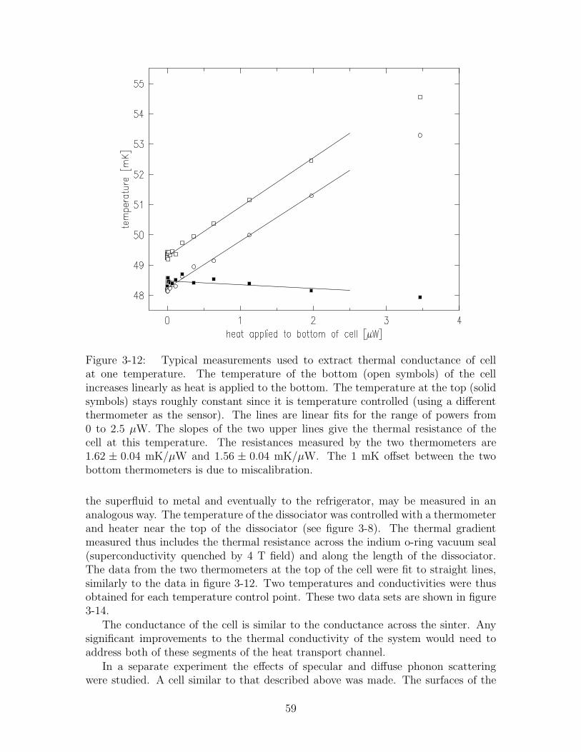
Figure 3-12: Typical measurements used to extract thermal conductance of cellat one temperature. The temperature of the bottom (open symbols) of the cellincreases linearly as heat is applied to the bottom. The temperature at the top (solidsymbols) stays roughly constant since it is temperature controlled (using a differentthermometer as the sensor). The lines are linear fits for the range of powers from0 to 2.5 µW. The slopes of the two upper lines give the thermal resistance of thecell at this temperature. The resistances measured by the two thermometers are1.62 ± 0.04 mK/µW and 1.56 ± 0.04 mK/µW. The 1 mK offset between the twobottom thermometers is due to miscalibration.

the superfluid to metal and eventually to the refrigerator, may be measured in ananalogous way. The temperature of the dissociator was controlled with a thermometerand heater near the top of the dissociator (see figure 3-8). The thermal gradientmeasured thus includes the thermal resistance across the indium o-ring vacuum seal(superconductivity quenched by 4 T field) and along the length of the dissociator.The data from the two thermometers at the top of the cell were fit to straight lines,similarly to the data in figure 3-12. Two temperatures and conductivities were thusobtained for each temperature control point. These two data sets are shown in figure3-14.

The conductance of the cell is similar to the conductance across the sinter. Anysignificant improvements to the thermal conductivity of the system would need toaddress both of these segments of the heat transport channel.

In a separate experiment the effects of specular and diffuse phonon scatteringwere studied. A cell similar to that described above was made. The surfaces of the

59

Figure 3-13: Thermal conductance along the length of the cell. The two data sets arefrom the two thermometers at the bottom of the cell. Approaching low temperaturesone expects the conductance to fall like T 3, as indicated by the line. The insetshows the conductance with this T 3 dependence factored out. The error bars are thestatistical fit uncertainties, and do not include systematics. The vertical error barsin the inset are dominated by the temperature uncertainty. Data without error barshave uncertainties smaller than the symbols.

bottom 23 cm of both the inner and outer tubes were sanded with 120 grit paperto create an optically dull finish. The remaining 42 cm exhibited the shiny surfacecharacteristic of the epoxy coating. The thermal conductance of the two sections wasmeasured in the range 50 mK to 300 mK. The section with diffuse optical reflectionhad a conductance three times lower than the other section. We thus conclude thatdiffuse reflection reduces the conductivity by a factor of 3 × 42/23 ≃ 5.

3.4.3 Heat Capacity

The heat capacity of the cell and dissociator have been measured together in a typ-ical trap loading sequence. The dissociator was held by a temperature controller at280 mK for 7 sec while pulsing an rf discharge inside. The heater and discharge wherethen turned off, and the cell plus dissociator assembly was cooled. The temperatureof the bottom of the cell is shown in figure 3-15. The cooling rate is expected to bedominated by the large heat capacities of the large copper pieces which comprise thedissociator and mixing chamber. Note that the molar specific heats of copper and

60

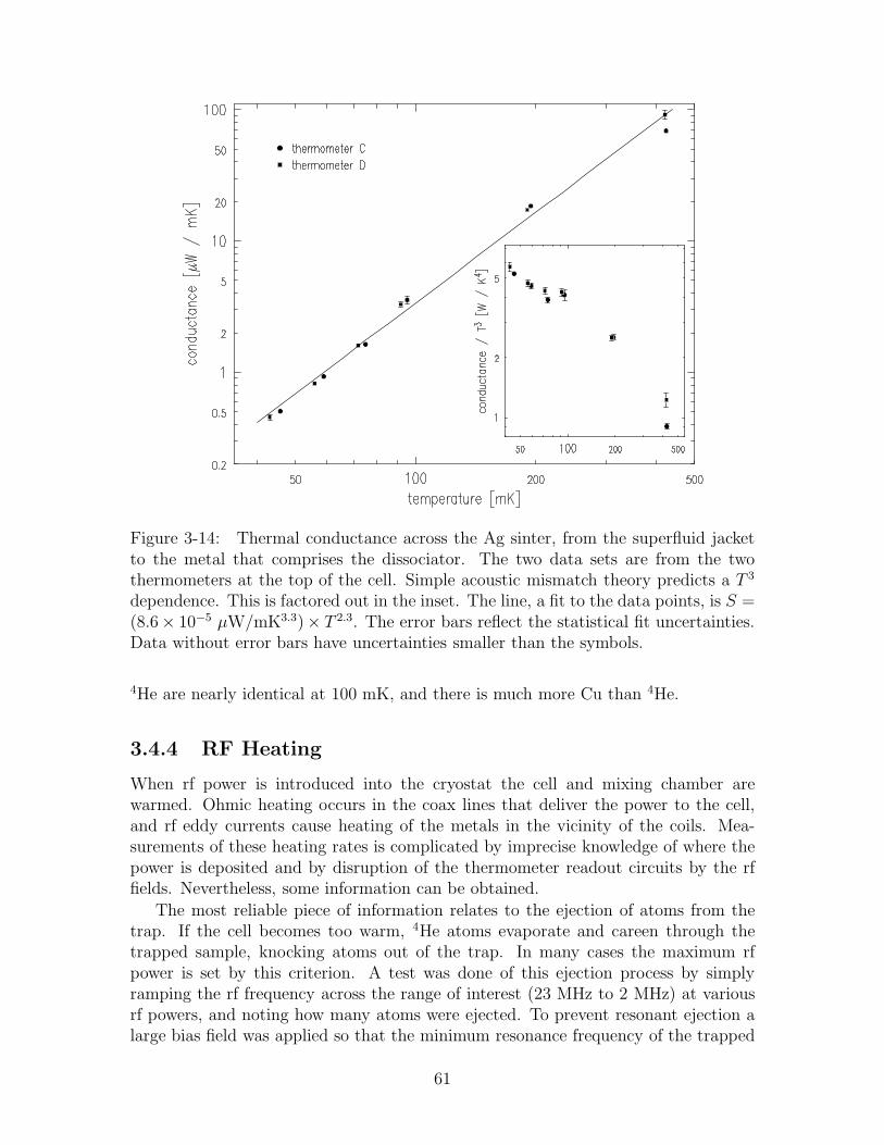
Figure 3-14: Thermal conductance across the Ag sinter, from the superfluid jacketto the metal that comprises the dissociator. The two data sets are from the twothermometers at the top of the cell. Simple acoustic mismatch theory predicts a T 3

dependence. This is factored out in the inset. The line, a fit to the data points, is S =(8.6× 10−5 µW/mK3.3)× T 2.3. The error bars reflect the statistical fit uncertainties.Data without error bars have uncertainties smaller than the symbols.

4He are nearly identical at 100 mK, and there is much more Cu than 4He.

3.4.4 RF Heating

When rf power is introduced into the cryostat the cell and mixing chamber arewarmed. Ohmic heating occurs in the coax lines that deliver the power to the cell,and rf eddy currents cause heating of the metals in the vicinity of the coils. Mea-surements of these heating rates is complicated by imprecise knowledge of where thepower is deposited and by disruption of the thermometer readout circuits by the rffields. Nevertheless, some information can be obtained.

The most reliable piece of information relates to the ejection of atoms from thetrap. If the cell becomes too warm, 4He atoms evaporate and careen through thetrapped sample, knocking atoms out of the trap. In many cases the maximum rfpower is set by this criterion. A test was done of this ejection process by simplyramping the rf frequency across the range of interest (23 MHz to 2 MHz) at variousrf powers, and noting how many atoms were ejected. To prevent resonant ejection alarge bias field was applied so that the minimum resonance frequency of the trapped

61

Figure 3-15: Temperature of the bottom of the cell while cooling from 280 mK.The cooling rate is dominated by the heat capacity of other metal parts, not thesuperfluid.

atoms was always above the applied rf frequency. No ejection was noted for powersup to +27 dBm outside the cryostat (corresponding to about 30 mG fields). Thecell thermometers indicated 220 mK (bottom) and 180 mK (top). The maximum rfpowers used for the experiments in this thesis were +15 dBm, so ejection of atomsfrom the trap was not a problem.

Another piece of reliable data is that the cell will stay below 160 mK when rf fieldsof roughly 5 mG are applied at frequencies of 23 MHz and below. This temperatureis low enough to allow the cell to cool reasonably quickly to temperatures at whichatoms may be dumped out of the trap and analyzed.

We note that there are a few resonances at which significant heating occurs. Theseare above 25 MHz. One possible rf leak might occur where the superconductingtwisted pair is joined to the coax. Further investigations of where heating occursshould be pursued. Methods could include a consideration of how fast objects coolwhen the rf is turned off and the time required for heat to reach various thermometers.

62

Chapter 4

Manipulating Cold Hydrogen by

RF Resonance

Resonant RF ejection of atoms from the trap is a tool for manipulating and studyingthe hydrogen gas. This tool has not previously been applied to trapped hydrogen, andso the peculiarities of this system have not been explored. We find—as anticipated—that rf ejection can efficiently remove energetic atoms that would otherwise not findtheir way out of the trap over the magnetic saddlepoint barrier. Experiments aredescribed in section 4.1. Furthermore, we find that rf ejection spectroscopy canconstitute a valuable diagnostic technique near BEC, where the trap dump techniqueused previously fails. RF ejection spectroscopy is also an essential tool for measuringthe magnetic field at the bottom of the trapping potential. These topics are coveredin section 4.2.

4.1 RF Evaporation

4.1.1 Need for RF Evaporation: Orbits with Long Escape

Times

In section 2.1 we explained that, for low temperature samples in tightly compressedtraps, the saddlepoint evaporation technique leads to one dimensional evaporation.Recall that atoms with high radial energy are unable to escape before having a colli-sion. In this section we demonstrate this problem experimentally.

Three successive samples are identically prepared by cooling into a trap withdepth ǫt/kB = 1.1 mK, set by a magnetic saddlepoint. The trap radial gradient isα/kB = 4.4 mK/cm. After the evaporation cycle is completed, the sample is heldfor many seconds (∼ 20), on the order of three characteristic collision times. Thesaddlepoint barrier is then reduced to zero in 5 s while the atom flux is recordedas a function of barrier height by sensing the heat of molecular recombination ona sensitive bolometer (section 4.2.3). In its simplest interpretation, this flux profileis the energy distribution of the trapped cloud. (Corrections to this picture will bedescribed in section 4.2.1). Figure 4-1 shows atom flux profiles for the three samples.

63

Figure 4-1: Comparison of dump signals from samples with and without rf ejection.The solid sloping line shows the trap depth as it is reduced from 1.1 mK to zero.The curves indicate the atom flux as the trap depth is reduced. The dashed curvescorrespond to a samples that were exposed to rf tuned to the trap depth for 9 s and23 s. The solid curve corresponds to a sample with no rf exposure. The rf fields ejecta sizeable fraction of the sample and change the shape of the profile. The responsetime of the detection process is seen at the end of the ramp, at t=5 s.

The largest profile is for a sample (sample 1) that was held for 10 s, and then dumpedfrom the trap. For the smaller two profiles, a weak rf field resonant at the trap depth(ǫt = hνrf − θ) was applied for 9 s (sample 2) and 23 s (sample 3) at the point inthe sequence where sample 1 was held. The samples were then dumped out of thetrap in the same way as sample 1. We see that a significant fraction of the atomshave been ejected from samples 2 and 3. To be ejected, these atoms must have had atotal energy that was above the magnetic saddlepoint energy. Since these atoms didnot leave the trap in sample 1, they were apparently in orbits with escape times of atleast ten seconds. This experiment demonstrates the long times required for energeticatoms to escape when the energy barrier is set only by a magnetic field saddlepointat one end of the trap, and the reduction in escape time when the atoms can leavein any direction. Furthermore, the decrease in trap population between samples 2and 3 indicates the long thermalization time of the system as it equilibrates to thelower effective trap depth for the radial degrees of freedom. This trap had a radialconfinement that was a factor of ∼ 3 weaker than those used for attaining BEC asdescribed in section 5.2, and so these experiments place a lower bound on the problem.

64

Figure 4-2: Demonstration of slow transfer of energy from axial to transverse mo-tional degrees of freedom. The five curves are the flux of atoms escaping the trap asthe magnetic energy barrier at one end of the trap is slowly ramped to zero (linearlysloping line), for each of five samples. The samples labeled 1-4 correspond to vari-ous durations of exposure of the sample to 10 MHz rf fields with strengths of a fewmilligauss. Sample 5 was confined in a short trap, and was exposed to an rf field at10 MHz for 20 s. The field had ten times more power than for samples 1-4.

4.1.2 Mixing of Energy

It is postulated that there is only very weak coupling among the motional degreesof freedom of a particle moving in the trap potential. This weak coupling betweentransverse and axial degrees of freedom is the impetus for driving evaporation with rffields. In this section we describe a simple experiment which demonstrates this veryweak coupling.

Four identically prepared samples are each cooled into a trap with depth ǫt =1.1 mK and radial gradient α = 4.5 mK/cm. The trap is significantly longer thanthe one shown in figure 3-4, with the sample extending from roughly z = −6 cmto z = +9 cm. The sample is adiabatically expanded by opening the trap slowly,reducing the radial gradient to α = 1.3 mK/cm, but leaving the length constant. Thepeak sample density is approximately n0 = 4 × 1012 cm−3. The thermalization timeis thus on the order of 10 s, and the dipolar decay time is on the order of 103 s.

Figure 4-2 shows the flux of atoms escaping the trap as the magnetic confinementfield at one end of the trap is linearly ramped to zero. As explained above, thisatom flux can be interpreted as an indication of the distribution of energies of the

65

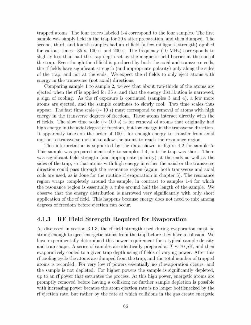
trapped atoms. The four traces labeled 1-4 correspond to the four samples. The firstsample was simply held in the trap for 20 s after preparation, and then dumped. Thesecond, third, and fourth samples had an rf field (a few milligauss strength) appliedfor various times—35 s, 100 s, and 200 s. The frequency (10 MHz) corresponds toslightly less than half the trap depth set by the magnetic field barrier at the end ofthe trap. Even though the rf field is produced by both the axial and transverse coils,the rf fields have significant strength (and appropriate polarity) only along the sidesof the trap, and not at the ends. We expect the rf fields to only eject atoms withenergy in the transverse (not axial) directions.

Comparing sample 1 to sample 2, we see that about two-thirds of the atoms areejected when the rf is applied for 35 s, and that the energy distribution is narrowed,a sign of cooling. As the rf exposure is continued (samples 3 and 4), a few moreatoms are ejected, and the sample continues to slowly cool. Two time scales thusappear. The fast time scale (∼ 10 s) must correspond to removal of atoms with highenergy in the transverse degrees of freedom. These atoms interact directly with therf fields. The slow time scale (∼ 100 s) is for removal of atoms that originally hadhigh energy in the axial degree of freedom, but low energy in the transverse direction.It apparently takes on the order of 100 s for enough energy to transfer from axialmotion to transverse motion to allow the atoms to reach the resonance region.

This interpretation is supported by the data shown in figure 4-2 for sample 5.This sample was prepared identically to samples 1-4, but the trap was short. Therewas significant field strength (and appropriate polarity) at the ends as well as thesides of the trap, so that atoms with high energy in either the axial or the transversedirection could pass through the resonance region (again, both transverse and axialcoils are used, as is done for the routine rf evaporation in chapter 5). The resonanceregion wraps completely around the sample, in contrast to samples 1-4 for whichthe resonance region is essentially a tube around half the length of the sample. Weobserve that the energy distribution is narrowed very significantly with only shortapplication of the rf field. This happens because energy does not need to mix amongdegrees of freedom before ejection can occur.

4.1.3 RF Field Strength Required for Evaporation

As discussed in section 3.1.3, the rf field strength used during evaporation must bestrong enough to eject energetic atoms from the trap before they have a collision. Wehave experimentally determined this power requirement for a typical sample densityand trap shape. A series of samples are identically prepared at T ∼ 70 µK, and thenevaporatively cooled to a given trap depth using rf fields of varying power. After thisrf cooling cycle the atoms are dumped from the trap, and the total number of trappedatoms is recorded. For very low rf powers essentially no rf evaporation occurs, andthe sample is not depleted. For higher powers the sample is significantly depleted,up to an rf power that saturates the process. At this high power, energetic atoms arepromptly removed before having a collision; no further sample depletion is possiblewith increasing power because the atom ejection rate is no longer bottlenecked by therf ejection rate, but rather by the rate at which collisions in the gas create energetic

66

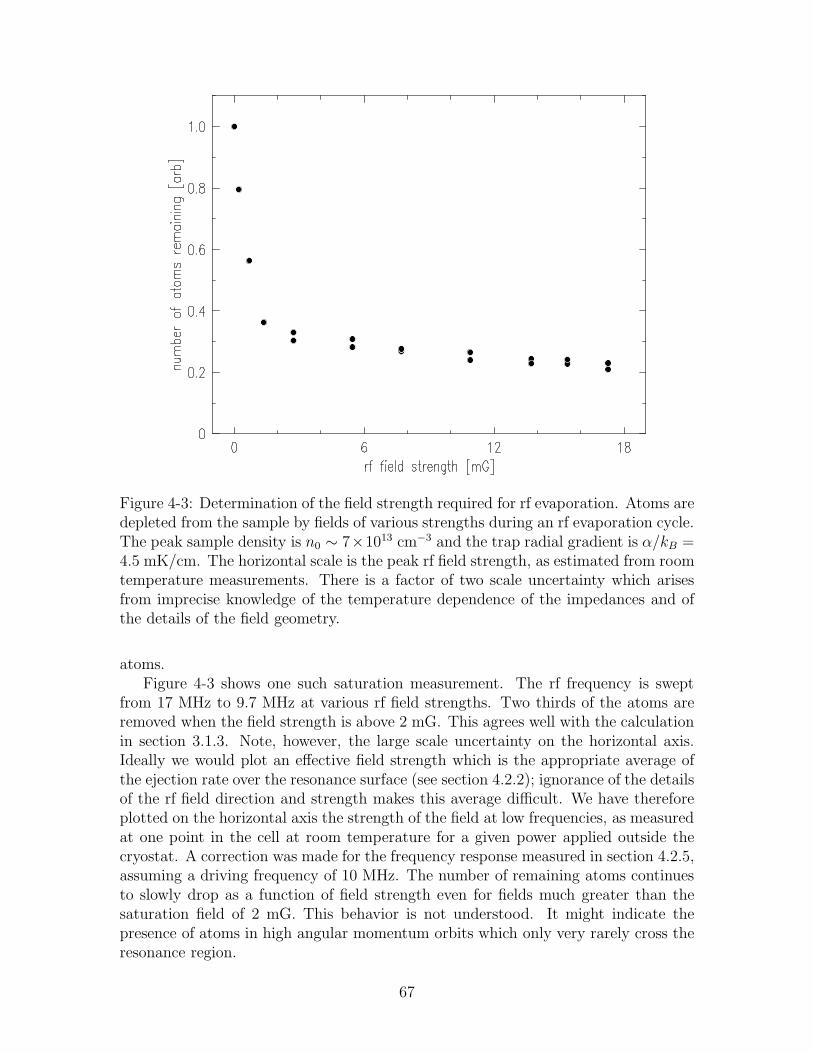
Figure 4-3: Determination of the field strength required for rf evaporation. Atoms aredepleted from the sample by fields of various strengths during an rf evaporation cycle.The peak sample density is n0 ∼ 7×1013 cm−3 and the trap radial gradient is α/kB =4.5 mK/cm. The horizontal scale is the peak rf field strength, as estimated from roomtemperature measurements. There is a factor of two scale uncertainty which arisesfrom imprecise knowledge of the temperature dependence of the impedances and ofthe details of the field geometry.

atoms.Figure 4-3 shows one such saturation measurement. The rf frequency is swept

from 17 MHz to 9.7 MHz at various rf field strengths. Two thirds of the atoms areremoved when the field strength is above 2 mG. This agrees well with the calculationin section 3.1.3. Note, however, the large scale uncertainty on the horizontal axis.Ideally we would plot an effective field strength which is the appropriate average ofthe ejection rate over the resonance surface (see section 4.2.2); ignorance of the detailsof the rf field direction and strength makes this average difficult. We have thereforeplotted on the horizontal axis the strength of the field at low frequencies, as measuredat one point in the cell at room temperature for a given power applied outside thecryostat. A correction was made for the frequency response measured in section 4.2.5,assuming a driving frequency of 10 MHz. The number of remaining atoms continuesto slowly drop as a function of field strength even for fields much greater than thesaturation field of 2 mG. This behavior is not understood. It might indicate thepresence of atoms in high angular momentum orbits which only very rarely cross theresonance region.

67

4.2 RF Ejection Spectroscopy

The simple technique of rf ejection spectroscopy is useful as a diagnostic of the tem-perature and density of the trapped gas near BEC. It has significant advantages overthe trap dump technique used previously, which becomes completely ambiguous nearthe BEC threshold. For probing the condensate, the technique is inferior to opticalspectroscopy (described in section 5.1.1), but it is much simpler to use. In this sectionwe explain the problems which make the trap dump technique ambiguous. We thendevelop a theory that explains the rf ejection measurements. After an explanation ofthe bolometric detection process employed in the rf ejection spectroscopy, we showhow the technique can be used to measure the magnetic field at the bottom of thetrap and to measure the temperature of a cold sample.

4.2.1 Ambiguities of the Trap Dump Technique

In previous experiments the sample was studied by dumping it from the trap andmeasuring its energy distribution (see section 2.5 and 2.6 in [17]); the distributionwas inferred by measuring the flux of escaping atoms as the axial trap barrier wasreduced (see figure 4-1 for example). Ambiguities arise, however, because of conflict-ing timescales. In order to measure an energy distribution, the flux detector mustrespond in a time τdet which is short compared to the duration over which the trapenergy threshold is reduced to zero, τdump. Furthermore, the characteristic sampleequilibration time, τequil, must be long compared to τdump so that the energy distri-bution does not change during the dump process. For the dense samples studied nearthe BEC transition the equilibration time is τequil ∼ 300 ms. The detector responsetime is τdet ∼ 200 ms. A further crippling complication is that the characteristicescape time, τesc, for an atom with total energy greater than the trap depth must beshort compared to τdump so that all of the atoms in a given energy slice leave the trapbefore atoms from the next slice begin to come out; in the tightly compressed trapsused near the BEC transition this escape time has been observed to be many tens ofseconds, as demonstrated by figure 4-1. The timescale hierarchy,

τdet, τesc ≪ τdump ≪ τequil (4.1)

is not achievable, and the trap dump technique fails to providing reliable measure-ments of the energy distribution of samples near the BEC regime. There is also apractical problem. As the axial confinement magnetic field is lowered, the trap shapechanges. Often a magnetic field zero forms, further complicating the measurements.

RF ejection spectroscopy, in which a resonance region is tuned through the trapto eject atoms with various potential energies, addresses all these problems. The trapshape remains unchanged, so no zeros are introduced. The particle escape time can beshort because atoms are coupled out in all directions. Finally, the energy distributionof the sample does not change significantly during the measurement process becauseonly a small fraction of the atoms are removed.

68

4.2.2 Theory of RF Ejection Spectroscopy of a Trapped Gas

In this section we use the results of the Landau-Zener theory discussed in section3.1.2 to explain the rf ejection spectrum expected for a trapped gas, i.e. the flux ofatoms ejected as a function of the frequency of the rf magnetic field. This expressionis used to interpret the spectra presented later in the chapter.

Consider a sample trapped in a magnetic potential V (r) = µB |Btrap(r)| describedby the potential energy density of states function (ε). The bottom of the trap isat a magnetic field B0 = θ/µB. An rf magnetic field, oscillating at frequency νrfwith strength Brf , is superimposed on the trap, and resonantly interacts with atomscrossing a surface of constant potential εres = hνrf − θ. For the analysis that followswe note that this surface area and its differential thickness is related to (ε) dε, whichis the differential volume in the trap with potential energy in a range dε around ε.This volume may be written as an integral, over the area of the surface of constantε, of the differential “thickness” dε/|α(r)| of the surface:

(ε) dε =∫

dAdε

|α(r)| (4.2)

where α(r) is the gradient of the potential at position r. This result will be used toderive equation 4.6.

We wish to find the rate at which atoms leave the trap as a result of Zeeman sub-level transitions in the resonance region. In a patch of resonance surface of differentialarea dA at position r, the differential atom loss rate is dN = FP dA, where F is theflux passing through the surface from either direction and P is the probability of theatom emerging from the resonance surface in an untrapped Zeeman sublevel. Equa-tions 3.23 and 3.24 indicate that, in the limit of low rf field strength, the vast majorityof transitions are made from the d to c Zeeman sublevels. The transition probabilityis P = Pc = 2(1 − p)p, where p = 1 − exp(−ζ) and ζ(r, v) = πµ2

BB2rf(r)/α(r)vh is

the adiabaticity parameter for an atom with velocity v passing through resonanceat a position r. Here Brf is the component of the rf field that is perpendicular tothe dc trapping field. In the weak field approximation, P ≃ 2p and p ≃ ζ . Thetransition probability exhibits a velocity dependence. The flux of atoms with velocityv passing through the surface is F (v) = n(r)fv(v)v where fv(v) is a normalized onedimensional velocity distribution function, such as derived in appendix E, and n(r)is the density at position r (either the Bose-Einstein or Maxwell-Boltzmann density,as appropriate). Since both P and F exhibit a velocity dependence, the differentialatom loss rate must be derived from an integral over velocities

dN = dA∫

dv n(r)f(v)v 2ζ(r, v)

= dA2πµ2

BB2rf(r)n(r)

|α(r)|h . (4.3)

The total atom loss rate F(ε), through a resonance surface at potential energy ε,

69

is

F(ε) =∫

dN

=2πµ2

Bn(ε)

h

∫

dAB2rf(r)

|α(r)| (4.4)

=2πµ2

B

hn(ε)B2

eff(ε)(ε). (4.5)

Here we have defined Beff as an effective rf field strength obtained by a weightedaverage, over the resonance surface, of the magnitude of the component of the rf fieldthat is orthogonal to the trapping field, Btrap. The weight function is the thicknessof the surface. Using equation 4.2

Beff (ε) ≡(

1

(ε)

∫

V (r)=εdA

(Brf(r) ×Btrap(r))2

|α(r)|B2trap(r)

)1/2

. (4.6)

If the polarization of Brf is randomized all over the resonance surface, then the crossproduct in equation 4.6 is essentially a scalar product, and Beff(ε) is the average, overthe equipotential surface, of the square of the rf field strength. This approximationis similar to a random phase approximation. Furthermore, if the length scale forvariations in the field strength is significantly different from the size of the trap, thenthe field averaged over the surface will be independent of the equipotential chosen.Certainly if the field is uniform over the trap (characteristic length long comparedto size of trap), then the average of the field over the equipotential surface does notdepend on which surface is chosen. In the other limit, if the characteristic lengthscale of the fluctuations in the field strength is short compared to the size of the trap,then the variations average out over the surface regardless of the surface chosen. Theresult in either case is that Beff is independent of ε. The field generated in the cellby a given rf driving power, measured outside the cryostat, can vary as a functionof frequency; this “transfer function” is an artifact of the reactance of the coils andthe drive line impedance, and is measured in section 4.2.5. This dependence is notincluded here.

In our experiment these two approximations (random orientation and incommen-surate length scale) are not so bad; the rf field is a superposition of the fields generatedby both the transverse and axial coils. The strength of the axial field varies on a lengthscale much shorter than the trap length, but much longer than the trap diameter,due to the field compensation scheme employed. Figure 3-4 shows the strength ofthe axial field along the symmetry axis of the trap. The field of the transverse coilis essentially uniform all across the trap. Since the relative strengths of the rf fieldcomponents vary all over the trap, the direction of the field also varies. Tests of thissimplifying assumption are outlined in section 4.2.5. The relative phase of the axialand transverse field is assumed to be zero, independent of frequency and position.Violations of this assumption have not been considered.

If Beff has no strong dependence on ε, then the flux of atoms ejected from the

70

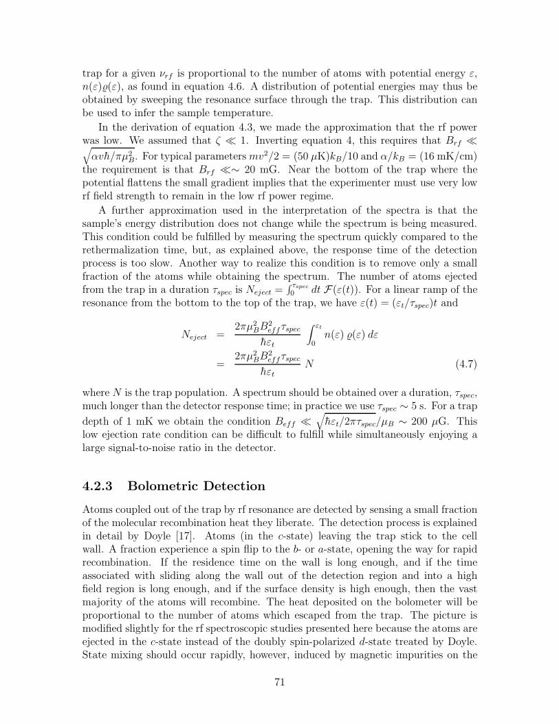
trap for a given νrf is proportional to the number of atoms with potential energy ε,n(ε)(ε), as found in equation 4.6. A distribution of potential energies may thus beobtained by sweeping the resonance surface through the trap. This distribution canbe used to infer the sample temperature.

In the derivation of equation 4.3, we made the approximation that the rf powerwas low. We assumed that ζ ≪ 1. Inverting equation 4, this requires that Brf ≪√

αvh/πµ2B. For typical parameters mv2/2 = (50 µK)kB/10 and α/kB = (16 mK/cm)

the requirement is that Brf ≪∼ 20 mG. Near the bottom of the trap where thepotential flattens the small gradient implies that the experimenter must use very lowrf field strength to remain in the low rf power regime.

A further approximation used in the interpretation of the spectra is that thesample’s energy distribution does not change while the spectrum is being measured.This condition could be fulfilled by measuring the spectrum quickly compared to therethermalization time, but, as explained above, the response time of the detectionprocess is too slow. Another way to realize this condition is to remove only a smallfraction of the atoms while obtaining the spectrum. The number of atoms ejectedfrom the trap in a duration τspec is Neject =

∫ τspec

0 dt F(ε(t)). For a linear ramp of theresonance from the bottom to the top of the trap, we have ε(t) = (εt/τspec)t and

Neject =2πµ2

BB2effτspec

hεt

∫ εt

0n(ε) (ε) dε

=2πµ2

BB2effτspec

hεtN (4.7)

where N is the trap population. A spectrum should be obtained over a duration, τspec,much longer than the detector response time; in practice we use τspec ∼ 5 s. For a trap

depth of 1 mK we obtain the condition Beff ≪√

hεt/2πτspec/µB ∼ 200 µG. Thislow ejection rate condition can be difficult to fulfill while simultaneously enjoying alarge signal-to-noise ratio in the detector.

4.2.3 Bolometric Detection

Atoms coupled out of the trap by rf resonance are detected by sensing a small fractionof the molecular recombination heat they liberate. The detection process is explainedin detail by Doyle [17]. Atoms (in the c-state) leaving the trap stick to the cellwall. A fraction experience a spin flip to the b- or a-state, opening the way for rapidrecombination. If the residence time on the wall is long enough, and if the timeassociated with sliding along the wall out of the detection region and into a highfield region is long enough, and if the surface density is high enough, then the vastmajority of the atoms will recombine. The heat deposited on the bolometer will beproportional to the number of atoms which escaped from the trap. The picture ismodified slightly for the rf spectroscopic studies presented here because the atoms areejected in the c-state instead of the doubly spin-polarized d-state treated by Doyle.State mixing should occur rapidly, however, induced by magnetic impurities on the

71

Figure 4-4: Impulse response of detection system. An rf pulse is applied for 200 ms,and the resulting bolometer signal is recorded. For this pulse the fit delay timeis τdelay = 277 ms, the fall time is τfall = 340 ms, and the effective rise time isτrise = 251 ms. The heat in this pulse is 2.6 pJ, which corresponds to the heatfrom 3 × 106 recombination events. The quiescent power applied to the bolometerwas 100 pW, the bolometer temperature was 180 mK, and the cell temperature was90 mK.

walls, and so the remaining considerations are still valid. They indicate that thecell walls should be cold (80 mK) and that the atom flux should be high. Both ofthese conditions impose limitations on the techniques described here. We observewell resolved rf spectra with atom fluxes on the order of 109 atoms per second fallingout of the trap toward the bolometer.

Crucial to the interpretation of the spectra presented is an understanding of thetime response of the bolometric detection process, as suggested above. The impulseresponse function of the detection system was measured directly using a series of200 ms rf pulses at various frequencies for samples of two different temperatures inthe range of interest. Figure 4-4 shows a typical pulse and an analytic fit of the form

g(t′) =

g0

τfall−τrise

(

e−t′/τfall − e−t

′/τrise

)

t′ ≥ 0

0 t′ < 0(4.8)

where t′ = t− τdelay. This form was chosen to model the time constants for an atomto stick to the wall and to find a recombination partner. The fit parameters were

72

consistent to about 10% for all the pulses, and the average values were τdelay = 299 ms,τrise = 246 ms, and τfall = 337 ms. The dependence of these parameters on the filmthickness has not been studied systematically, but at low film thicknesses the H-Hebinding energy increases and the atoms stick promptly; τdelay decreases. Becausethe rf pulse has finite duration, the measured response is not, strictly speaking, theimpulse response function. Nevertheless, it is a good approximation, and the analyticfit parameters quoted above were used in calculating the spectra presented in thefollowing sections.

The response time of the bolometer readout electronics was measured by heatingthe bolometer with short pulses of light from a HeNe laser. The response time wasapproximately 10−3 s, negligible compared to the time constants for recombination.

4.2.4 Measuring the Trap Bias Field

The bias field in the Ioffe-Pritchard trap, θ/µB, sets the characteristic sample tem-perature at which the trap functional form changes from predominantly linear (T ≫θ/kB) to predominantly harmonic (T ≪ θ/kB) in the two radial dimensions. It is thusan important quantity for analysis of Bose condensation experiments. Furthermore,to know the trap depth ǫt = hνrf − θ, one must know both the trap energy barrier(set by the experimenter) and the bias energy.

The bias is directly measured by sweeping up the frequency of the rf field untilatoms begin to be ejected from the trap. Figure 4-5 shows such a sweep. The atomsbegin to be coupled out of the trap at about t = 5 s, corresponding to a frequencyνθ = 700 kHz; in this case we find θ/kB = νθh/kB = 33.6 µK. RF ejection is apowerful and sensitive technique to quickly and accurately measure the absolute trapbias.

The bias can also be inferred by deforming the trap potential until a field zerois created; atoms begin to experience Majorana flips, leave the bottom of the trap,and get detected by the bolometer. The zero is made by changing the current in asolenoid that creates a fairly uniform field along the length of the trap. Integration ofthe Biot-Savart law gives the field strength per unit current. This method of findingthe bias field is not as accurate as the rf ejection method since the trap shape isdeformed for the measurement. Nevertheless, the two methods agree to within theexperimental uncertainties.

4.2.5 Measuring the Effective RF Field Strength

In order to analyze rf ejection spectra, one must know the effective rf field strength,Beff given by equation 4.6. It may exhibit complicated polarization dependences ifthe random orientation and incommensurate length scale approximations made inthe discussion of equation 4.6 are invalid. Furthermore, there may be a frequencydependence in the field strength generated in the cell by a given rf power appliedoutside the cryostat, as discussed in section 3.4.1. Clearly a measurement of theefficiency is in order.

73

Figure 4-5: Measurement of trap bias using rf ejection. The rf field is switched onat t = 0 and swept from 200 kHz to 1.2 MHz. The atoms begin to leave the trap atabout 700 kHz. The sloping baseline signal results from atoms evaporating out of thetrap as the sample continues to cool after the end of the forced evaporative coolingcycle.

RF spectra were measured to verify the ejection efficiency for frequencies between1 and 17 MHz. The ejection rate at a given frequency, given by equation 4.5, includesthe density, the potential energy density of states, and the effective rf field strength.In order to simplify the measurement of the efficiency, the density was kept constantover the energy range of interest by using a warm sample, T ∼ 1 mK> hνmax/kB.The potential energy density of states functional form is known well. The quantityobtained, then, is the ejection efficiency as a function of frequency. The flux ejectedas the frequency of the rf field was swept upward is shown in figure 4-6 for the axialcoil alone, the transverse coil alone, and both coils together. Another sweep, takenwith no atoms in the trap but with both coils driven, indicates rf pickup and heatingeffects.

The simplest model of the frequency dependence of the ejection efficiency ignorespolarization effects and accounts only for impedance matching (the voltage dividereffects of the reactance of the coils and the 50 Ω feed lines); we take

Beff (ω) ∝∣∣∣∣∣

1

1 + iω/ω0

∣∣∣∣∣

(4.9)

74

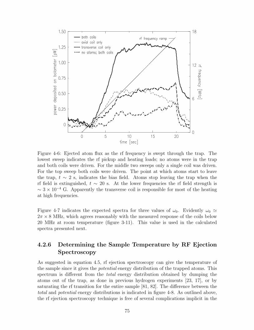
Figure 4-6: Ejected atom flux as the rf frequency is swept through the trap. Thelowest sweep indicates the rf pickup and heating loads; no atoms were in the trapand both coils were driven. For the middle two sweeps only a single coil was driven.For the top sweep both coils were driven. The point at which atoms start to leavethe trap, t ∼ 2 s, indicates the bias field. Atoms stop leaving the trap when therf field is extinguished, t ∼ 20 s. At the lower frequencies the rf field strength is∼ 3 × 10−4 G. Apparently the transverse coil is responsible for most of the heatingat high frequencies.

Figure 4-7 indicates the expected spectra for three values of ω0. Evidently ω0 ≃2π × 8 MHz, which agrees reasonably with the measured response of the coils below20 MHz at room temperature (figure 3-11). This value is used in the calculatedspectra presented next.

4.2.6 Determining the Sample Temperature by RF Ejection

Spectroscopy

As suggested in equation 4.5, rf ejection spectroscopy can give the temperature ofthe sample since it gives the potential energy distribution of the trapped atoms. Thisspectrum is different from the total energy distribution obtained by dumping theatoms out of the trap, as done in previous hydrogen experiments [23, 17], or bysaturating the rf transition for the entire sample [81, 82]. The difference between thetotal and potential energy distributions is indicated in figure 4-8. As outlined above,the rf ejection spectroscopy technique is free of several complications implicit in the

75

Figure 4-7: Determination of the frequency response of the coils by a comparisonof calculated and measured spectra. The measured spectrum has the background,shown in figure 4-6, subtracted. The only adjustable parameters in the calculatedspectra are the overall normalization, the baseline, and ω0.

trap dump technique. RF ejection spectroscopy has been employed to measure thetemperature of the coldest samples of trapped H to date, a factor of 40 colder thanthe photon recoil cooling limit.

Figure 4-9 shows the spectrum of a sample that was cooled to T = 30 µK byrf evaporation. This sample should contain a small condensate, although it is notvisible here. The three calculated spectra in figure 4-9 assume quantum degeneracy.Furthermore, they include the measured time response of the detection system, themeasured trap bias, and the measured effective rf field strength. Possible distortions,not considered in the calculations, arise from sample depletion during the rf sweepand changing detection sensitivity due to nonlinearities in the detection process atlow atom fluxes. This second effect should be small, as suggested by the qualityof the calculated rf ejection spectrum, which ignored nonlinearity. The first effectcan be shown to be small by taking a series of such spectra at various rf powers,thus depleting the sample by various (small) amounts. Of course at lower powersthe signal/noise ratio becomes smaller; the power used for the spectrum in figure 4-9involves a compromise between signal size and distortion. The apparent temperatureis shifted no more than 10%.

Determination of sample temperature through rf ejection spectroscopy is limitedby the signal rate, which is proportional to Neject/τspec in equation 4.7. The technique

76

Figure 4-8: Probing the distribution of total energy and potential energy of a trappedsample. The total (potential) energy distribution function gives the number of par-ticles with a given total (potential) energy. The shaded area is the region of atomsprobed by the technique. The solid lines indicate the trapping potential, and thedashed line is the trap depth.

could be extended to much lower temperatures if the detection efficiency is improved.A practical limitation involves the requirement that the cell walls be cold enough to

support a long atom residence time, and thus high recombination efficiency. Becauseof rf heating effects, this limitation usually requires the rf power to be reduced forseveral seconds before the rf spectrum is obtained. The sample can warm during thistime since the trap depth is not as well defined.

77

Figure 4-9: RF spectrum of trapped gas at 30 µK. The heavy line is the raw data.The thin solid line is the inferred background, whose functional form has been verifiedindependently. The three dashed lines are calculations of the spectrum for differenttemperatures assuming quantum degeneracy. The calculations include the time re-sponse of the detection system, the measured trap depth, and the measured effectiverf field strength. The only remaining adjustable parameter is the normalization. Therf field strength used for this spectrum is ∼ 200 µG.

78

Chapter 5

Observation of BEC

In this chapter we describe the first observations of Bose-Einstein condensation ofhydrogen.

Our primary diagnostic technique is laser spectroscopy, which we briefly describehere; detailed descriptions are given by Sandberg [16] and Killian [13] (Killian’s thesisshould be considered a companion to this chapter). With this probe we are able tomonitor the density and temperature of the gas as the temperature is reduced by rfevaporation. When the gas is cooled into the quantum degenerate regime signaturesof the Bose-Einstein condensate appear in the spectrum; these can be analyzed toreveal the size and population of the condensate. As anticipated, the condensate ishuge, containing a factor of 50 more atoms than condensates in other experiments,and having a length on the order of a centimeter. We are able to study the timeevolution of the condensate, which is governed by feeding of the condensate from thethermal gas. We explore some of the implications of these results for the productionof high-flux coherent atomic beams.

5.1 Laser Spectroscopy of Trapped Hydrogen

Laser spectroscopy of trapped atomic hydrogen has been pursued as both a techniqueto study and manipulate a trapped gas, and as a probe of the collection of individualatoms for metrology and fundamental measurements [24, 16, 14, 83]. We focus hereon spectroscopy as a tool to measure the density and temperature of the trapped gas.It has been suggested that the coherence properties of Bose-condensed atoms couldbe exploited to perform much improved fundamental measurements [84, 85].

The principal transition in hydrogen, 1S-2P , has a large transition rate, but isdifficult to use for sample diagnostics because it has a large linewidth (100 MHz),it suffers from complicated magnetic structure, and it is in the uv (121.6 nm). Thetransition has been used by the Amsterdam hydrogen trapping group as a diagnosticfor warm samples, and also for limited laser cooling and laser induced evaporation[86, 87, 88]. The Doppler effect can be used to measure the sample temperature,but the short 2P lifetime limits the technique to temperatures above a few mK.In order to circumvent the short 2P lifetime, the Amsterdam group employed two-

79

photon spectroscopy to the 3S (160 ns) and 3D (16 ns) states [89]. To enhance thetwo-photon transition rate, one photon was tuned near the Lyman-α resonance andthe other near the Balmer-α. In principle the 1S-3S transition could be used fortemperature measurement all the way into the sub-µK regime.

5.1.1 Spectroscopy of the 1S-2S Transition

We employ the 1S-2S transition and drive it with two photons at 243 nm, twice theLyman-α wavelength. The 2S state is metastable with lifetime τ0 = 120 ms, andthe natural linewidth is below 1 Hz. The transition thus constitutes a very sensitiveprobe, through shifts and broadenings, of the local environment of the atom. Asexplained below, the transition can be used to measure the density of the gas, inaddition to the temperature.

To excite the transition the laser beam is retroreflected to create a standing wavein the atom cloud. In this configuration the atom may absorb two photons from thesame beam or one photon from each beam. Absorption of co-propagating photonsinvolves the Doppler shift, and the excitation is said to be “Doppler-sensitive” (DS).In the absorption of counter-propagating photons the Doppler effect cancels to firstorder, and the process is termed “Doppler-free” (DF).

The energy equation for two-photon excitation of an isolated atom from state ito f , with initial momentum pi and final momentum pf = pi + h(k1 + k2), where k1

and k2 are the wave vectors of the laser beams, is

2hν =√

p2fc

2 + (mc2 + 2hνo)2 −√

p2i c

2 + (mc2)2. (5.1)

where the rest mass of the atom in the initial state is m and 2νo = 2.466 × 1015 Hz[90] is the unperturbed transition frequency. Expanding, we obtain

ν = νo +(k1 + k2) · pi

4πm(1 − ǫ)

︸ ︷︷ ︸

∆νD1

+h(k1 + k2)

2

8πm(1 − ǫ)

︸ ︷︷ ︸

∆νR

− νop2i

2(mc)2

︸ ︷︷ ︸

∆νD2

+O(ǫ3). (5.2)

Here ∆νD1 and ∆νD2 are the first and second order Doppler shifts, respectively, ∆νRis the recoil shift, and ǫ = 2hνo/mc

2 = 1.1 × 10−8 is a relativistic correction whichaccounts for the mass change of the atom upon absorbing energy 2hνo. For hydrogenin the submillikelvin regime, ∆νD2 ≪ 1 Hz and can be neglected. In the Doppler-sensitive configuration, k1 = k2 and ∆νR = 6.7 MHz. (All frequencies are referencedto the 243 nm laser source). At a temperature of 50 µK, ∆νD1 ∼ 2.6 MHz, and thusthe Doppler-sensitive peak is well separated from the Doppler-free. In the Doppler-free configuration, k1 = −k2, and there is no recoil or first order Doppler broadening.A spectrum is shown in figure 5-1.

A complete discussion of the shape of the Doppler-free line in the various regimesof density and temperature is presented in the thesis of Thomas Killian [13]. Wesummarize his discussion by noting that the narrow intrinsic linewidth allows thespectrum to be used for measuring the density and temperature of the sample. The

80

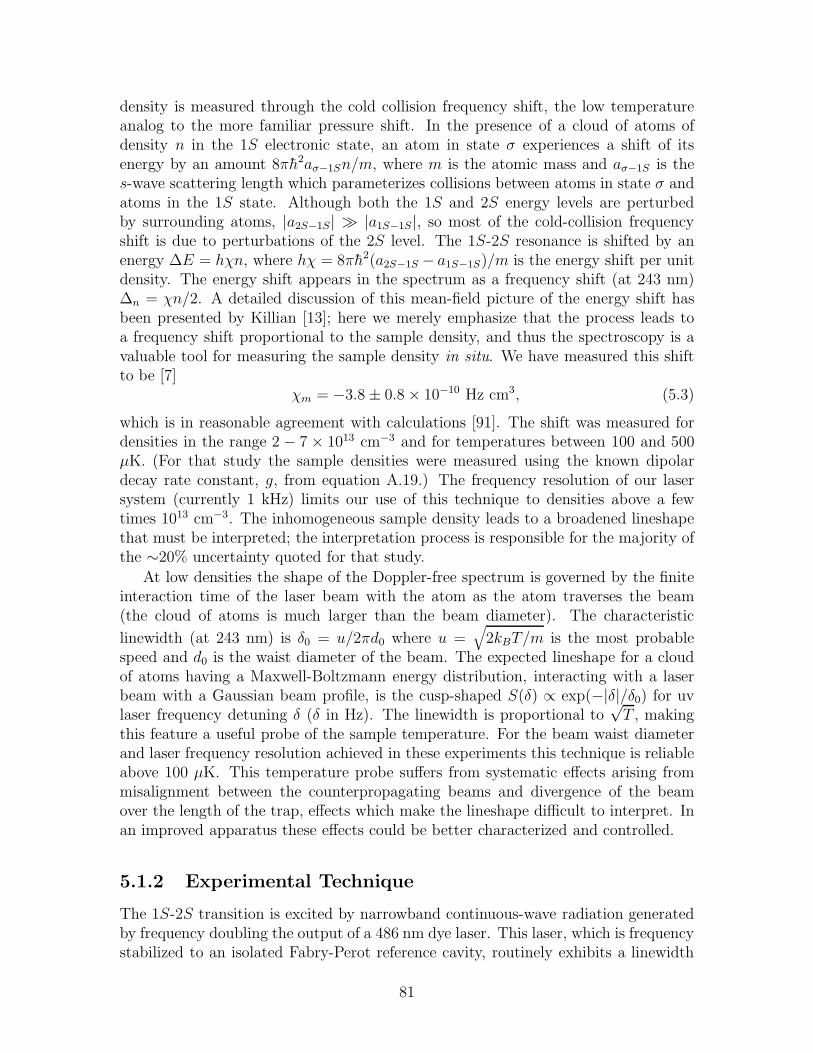
density is measured through the cold collision frequency shift, the low temperatureanalog to the more familiar pressure shift. In the presence of a cloud of atoms ofdensity n in the 1S electronic state, an atom in state σ experiences a shift of itsenergy by an amount 8πh2aσ−1Sn/m, where m is the atomic mass and aσ−1S is thes-wave scattering length which parameterizes collisions between atoms in state σ andatoms in the 1S state. Although both the 1S and 2S energy levels are perturbedby surrounding atoms, |a2S−1S| ≫ |a1S−1S|, so most of the cold-collision frequencyshift is due to perturbations of the 2S level. The 1S-2S resonance is shifted by anenergy ∆E = hχn, where hχ = 8πh2(a2S−1S − a1S−1S)/m is the energy shift per unitdensity. The energy shift appears in the spectrum as a frequency shift (at 243 nm)∆n = χn/2. A detailed discussion of this mean-field picture of the energy shift hasbeen presented by Killian [13]; here we merely emphasize that the process leads toa frequency shift proportional to the sample density, and thus the spectroscopy is avaluable tool for measuring the sample density in situ. We have measured this shiftto be [7]

χm = −3.8 ± 0.8 × 10−10 Hz cm3, (5.3)

which is in reasonable agreement with calculations [91]. The shift was measured fordensities in the range 2 − 7 × 1013 cm−3 and for temperatures between 100 and 500µK. (For that study the sample densities were measured using the known dipolardecay rate constant, g, from equation A.19.) The frequency resolution of our lasersystem (currently 1 kHz) limits our use of this technique to densities above a fewtimes 1013 cm−3. The inhomogeneous sample density leads to a broadened lineshapethat must be interpreted; the interpretation process is responsible for the majority ofthe ∼20% uncertainty quoted for that study.

At low densities the shape of the Doppler-free spectrum is governed by the finiteinteraction time of the laser beam with the atom as the atom traverses the beam(the cloud of atoms is much larger than the beam diameter). The characteristic

linewidth (at 243 nm) is δ0 = u/2πd0 where u =√

2kBT/m is the most probablespeed and d0 is the waist diameter of the beam. The expected lineshape for a cloudof atoms having a Maxwell-Boltzmann energy distribution, interacting with a laserbeam with a Gaussian beam profile, is the cusp-shaped S(δ) ∝ exp(−|δ|/δ0) for uvlaser frequency detuning δ (δ in Hz). The linewidth is proportional to

√T , making

this feature a useful probe of the sample temperature. For the beam waist diameterand laser frequency resolution achieved in these experiments this technique is reliableabove 100 µK. This temperature probe suffers from systematic effects arising frommisalignment between the counterpropagating beams and divergence of the beamover the length of the trap, effects which make the lineshape difficult to interpret. Inan improved apparatus these effects could be better characterized and controlled.

5.1.2 Experimental Technique

The 1S-2S transition is excited by narrowband continuous-wave radiation generatedby frequency doubling the output of a 486 nm dye laser. This laser, which is frequencystabilized to an isolated Fabry-Perot reference cavity, routinely exhibits a linewidth

81

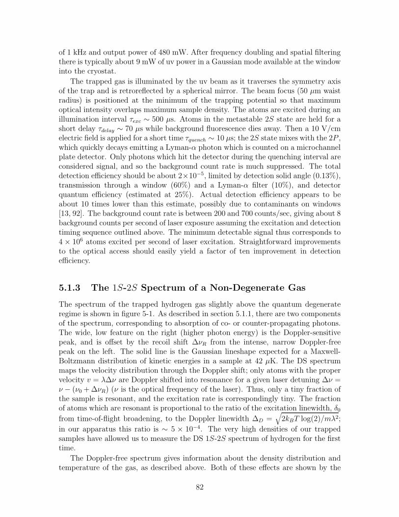
of 1 kHz and output power of 480 mW. After frequency doubling and spatial filteringthere is typically about 9 mW of uv power in a Gaussian mode available at the windowinto the cryostat.

The trapped gas is illuminated by the uv beam as it traverses the symmetry axisof the trap and is retroreflected by a spherical mirror. The beam focus (50 µm waistradius) is positioned at the minimum of the trapping potential so that maximumoptical intensity overlaps maximum sample density. The atoms are excited during anillumination interval τexc ∼ 500 µs. Atoms in the metastable 2S state are held for ashort delay τdelay ∼ 70 µs while background fluorescence dies away. Then a 10 V/cmelectric field is applied for a short time τquench ∼ 10 µs; the 2S state mixes with the 2P ,which quickly decays emitting a Lyman-α photon which is counted on a microchannelplate detector. Only photons which hit the detector during the quenching interval areconsidered signal, and so the background count rate is much suppressed. The totaldetection efficiency should be about 2×10−5, limited by detection solid angle (0.13%),transmission through a window (60%) and a Lyman-α filter (10%), and detectorquantum efficiency (estimated at 25%). Actual detection efficiency appears to beabout 10 times lower than this estimate, possibly due to contaminants on windows[13, 92]. The background count rate is between 200 and 700 counts/sec, giving about 8background counts per second of laser exposure assuming the excitation and detectiontiming sequence outlined above. The minimum detectable signal thus corresponds to4 × 106 atoms excited per second of laser excitation. Straightforward improvementsto the optical access should easily yield a factor of ten improvement in detectionefficiency.

5.1.3 The 1S-2S Spectrum of a Non-Degenerate Gas

The spectrum of the trapped hydrogen gas slightly above the quantum degenerateregime is shown in figure 5-1. As described in section 5.1.1, there are two componentsof the spectrum, corresponding to absorption of co- or counter-propagating photons.The wide, low feature on the right (higher photon energy) is the Doppler-sensitivepeak, and is offset by the recoil shift ∆νR from the intense, narrow Doppler-freepeak on the left. The solid line is the Gaussian lineshape expected for a Maxwell-Boltzmann distribution of kinetic energies in a sample at 42 µK. The DS spectrummaps the velocity distribution through the Doppler shift; only atoms with the propervelocity v = λ∆ν are Doppler shifted into resonance for a given laser detuning ∆ν =ν − (ν0 + ∆νR) (ν is the optical frequency of the laser). Thus, only a tiny fraction ofthe sample is resonant, and the excitation rate is correspondingly tiny. The fractionof atoms which are resonant is proportional to the ratio of the excitation linewidth, δ0from time-of-flight broadening, to the Doppler linewidth ∆D =

√

2kBT log(2)/mλ2;

in our apparatus this ratio is ∼ 5 × 10−4. The very high densities of our trappedsamples have allowed us to measure the DS 1S-2S spectrum of hydrogen for the firsttime.

The Doppler-free spectrum gives information about the density distribution andtemperature of the gas, as described above. Both of these effects are shown by the

82

Figure 5-1: Spectrum of non-degenerate gas. The intense narrow peak on the leftresults from Doppler-free excitation and the low broad peak on the right results fromDoppler-sensitive excitation which probes the velocity distribution. The solid lineon the right is the expected Doppler-sensitive spectrum for a nondegenerate sampleat 42 µK. At this low temperature the recoil-shifted Doppler-sensitive line is clearlyseparated from the Doppler-free line. The error bars are statistical. The ratio ofpeak heights should be taken as only a rough indication of the transition rate ratiosbecause of variations in laser power and beam alignment.

spectra in figure 5-2, just three of many successive spectra that were measured as thedensity of the sample slowly decayed. The initial spectra exhibit a large shift, arisingfrom the cold-collision frequency shift at high density. The inhomogeneous density inthe trap causes a broadening of the spectrum as well. As the sample density decreases,the shift and broadening also decrease. At low density, where the density-dependentshift is negligible, the exponential lineshape characteristic of transit time broadeningis evident. The frequency shift of the spectra of high density samples is used to obtainthe sample density, and the width of the transit-time broadened line is related to thesample temperature.

5.2 Cooling into the Degenerate Regime

Armed with an efficient cooling method (rf evaporation) and a sensitive probe ofsample density and temperature (spectroscopy), we are equipped to push toward the

83

Figure 5-2: Doppler-free spectra at various sample densities. The trap depth is570 µK, corresponding to a sample temperature T ∼ 70 µK. The spectra of thehigher density samples are red-shifted and broadened by the inhomogeneous density.The lines connecting the points are a guide to the eye. The samples were confined bytrap shape A, described in table 5.1. The highest density is about 1014 cm−3.

quantum degenerate regime. The trap is loaded as described in section 1.3, andthe sample is cooled by magnetic field saddlepoint evaporation. The currents inthe magnetic coils that create the trapping potential are ramped to slowly changethe trap from the deep, long, open shape used for loading the atoms to a short,tightly compressed, shallow trap from which rf evaporation is commenced. Figure 5-3indicates the process. In this section we discuss the path through density-temperaturespace taken by the sample as it is cooled into the quantum degenerate regime.

5.2.1 Cooling Paths

Previous attempts to achieve BEC in hydrogen were thwarted by inefficient evapora-tion at the lowest temperatures. In order to verify that we have solved this problem,the progress of the sample through phase space (density-temperature space) is mon-itored as the sample is cooled. We find that the sample is cooled efficiently. We alsofind and explore the phase boundary where the sample undergoes phase separationinto a condensate and normal gas. This first evidence for phase transition behavioris described below.

84

for initial loadinglong, open trap

saddlepointevaporation

density: 10 cm -320

temperature: 300 K

H2

room temperaturehydrogen gas

µtemperature: 50 K

cryogenics

0.5 K deep

(cm)ρ

field (G)

RFevaporation

z (cm)

density: 2x10 cm 14 -3

density: 6x10 cm -313

trap used for BEC

density: 2x10 cm 13 -3

temperature: 40 mK

(300 K deep)

(1.1 mK deep)

µ

µtemperature: 100 K

energetic atomsescape here

shallow, harmonicIoffe-Pritchard trap

Figure 5-3: Schematic diagram of trap shape as sample is loaded and evaporativelycooled to BEC. Room temperature molecular hydrogen (upper left diagram) is cooledto 275 mK by cryogenic techniques. It is dissociated, and the atoms are loaded into anopen, long trap that is about 500 mK deep (upper right diagram). The magnetic fieldin the ρ− z plane is shown. Note the very different scales for the radial coordinate ρand the axial coordinate z. During trap loading, the atoms settle into the region oflow field at the center of the trap. The sample is then cooled by magnetic saddlepointevaporation. It is compressed radially and axially into a trap that is nearly harmonicalong the z axis and predominantly linear along the radial axis (lower right diagram).It is this trap shape that is labeled “A” or “B” (see section 5.2.1). RF evaporationis used to further cool the sample while the trap shape remains fixed (lower leftdiagram). The entire cooling process takes about 5 minutes.

A series of measurements were made to map the sample’s trajectory through phasespace as it was cooled into the quantum regime. Identical samples were cooled into atrap of depth ǫt/kB = 1.1 mK. This process used magnetic saddlepoint evaporationexclusively. The trap shape was then held constant while the trap depth was reducedby rf evaporation. (Three trap shapes will be discussed in this chapter, A, A′, and

85

parameter trap A trap A′ trap B

α/kB (mK/cm) 15.9 9.5β/kB (µK/cm2) 25θ/kB (µK) 27 ± 2 35 ± 2 34 ± 2

n0(T = 120 µK) (×1013 cm−3) 8 1.7

Table 5.1: Summary of parameters describing the three trap shapes used in thischapter. The parameters α, β, and θ describe the Ioffe-Pritchard potential; α and βare calculated, and θ is measured. The peak density at T = 120 µK is noted.

B. Their characteristics are summarized in table 5.1. Here we refer to trap shapeA.) The evaporation path (the trap depth as a function of time) was identical for allsamples, but the different samples were taken various distances along the path. Therf frequency f(t) that sets the trap depth ǫt = hf(t)−θ was ramped according to thefunction1 f(t) = fstart(fend/fstart)

(t/d)ξwhere the start frequency is fstart = 23 MHz,

the end frequency is fend = 2 MHz, the maximum ramp duration is d = 25 s, andthe shape exponent ξ = 1.5. The ramp was executed for a duration τr. For t ≥ τr,the frequency was maintained at f(τr). Evaporation could still occur, but forcedevaporation halted. After rf evaporation was completed, the sample density wasmeasured using the cold-collision frequency shift of the DF spectrum as describedabove. The densities thus measured are shown in figure 5-4. The density initiallyincreases as the trap depth (and thus temperature) is reduced because the atoms areconfined to a smaller volume closer to the bottom of the trap. Some atoms are lostthrough evaporation, but the good efficiency of evaporative cooling leads to overallphase space compression. The cooling efficiency parameter γ = d logD/d logN (thephase space density is D ≡ n0Λ

3) is γ ≃ −1.5 during this stage of the cooling.

At a trap depth of about ǫt/kB = 280 µK the phase space trajectory exhibitsa dramatic kink. Further cooling leads to decreasing density in the normal gas;apparently population is being rapidly removed. The location of the kink and theslope of the subsequent trajectory agree well with the BEC phase transition line,nc = 2.612(2πmkBT )3/2/h3 assuming a ratio of trap depth to temperature of η =ǫt/kBT ∼ 6, which is reasonable. The “excluded region” above the line has thefollowing interpretation: as the sample is cooled, the thermal cloud cannot support apeak density above nc; extra atoms are transferred to the condensate. The condensateis not directly observed in these measurements because its density is so large (asdiscussed in section 5.3.1) that its spectrum is shifted far away from the spectrum ofthe thermal cloud.

The magnetic trap shape used for these experiments (trap shape A) was chosen asa compromise between high radial compression and adequate magnetic saddlepointevaporation efficiency. High radial compression is desirable because the correspond-ingly higher densities allow BEC to be reached at a higher temperature. As discussed

1The evaporation path was not optimized before most of the data presented in this chapter wasobtained. For future studies an optimization of the functional form of the path is desirable.

86

Figure 5-4: Path of non-condensed portion of the sample through n − T space asthe sample is cooled into the degenerate regime. Paths are shown for samples in twodifferent traps: open circles — trap A, closed circles — trap B. The trap depth is setby the frequency of the rf magnetic field, and above degeneracy the temperature isabout 1/η ∼ 1/8th the trap depth. The density is measured through the cold-collisionfrequency shift. The non-condensed portion of the sample cannot have density greaterthan the BEC critical density nc ∝ T 3/2, and thus the upper left region of the phasediagram is not accessible. The condensates created in the two traps contain aboutthe same number of atoms.

in section 5.2.2, evaporation and the approach to BEC should be more efficient athigher temperatures because the ratio of “good” to “bad” collisions is more favor-able. On the other hand, high radial compression is undesirable because the magneticfield saddlepoint evaporation process (see figure 5-3) that cools and compresses thesample into the tight trap is less efficient. As discussed in section 2.1, tight radialcompression leads to more regular motion of the trapped atoms, and thus to reducedevaporation dimensionality.

A more open trap, trap B, has also been used. A typical phase space trajectory isshown by the filled circles in figure 5-4 . The evaporation was done more slowly, withmaximum duration d = 55 s, but was otherwise identical to the path described above.The evaporation efficiency parameter is γ ∼ −2.7 for cooling above the degenerateregime. The higher evaporation efficiency has not been systematically studied, butcould arise simply because the trajectory duration d was optimized for trap B, butnot trap A.

87

Computer models of the cooling process have been constructed, and are describedin appendix D. The trajectories through phase space calculated by them are in goodagreement with observations.

5.2.2 Evaporation Strategies

There are many paths that can be taken through phase space to the BEC phaseboundary. In this section we discuss the experimental limitations of the presentapparatus and their implications for the choice of evaporation path.

As shown in section A.2.2, evaporation is more efficient in hydrogen at higher tem-peratures. There the ratio of “good” collisions to “bad” collisions is higher. “Good”collisions are those which lead to cooling, and they occur at a rate Γevap ∝ Γcol ∝nσv ∝ n

√T for a sample of density n. “Bad” collisions are those which lead to

dipolar relaxation and heating. They occur at a rate Γdip ∝ gn. The collision ratioΓevap/Γdip ∝

√T is higher at higher temperatures. More phase space compression

can be accomplished per atom lost from the trap. This higher efficiency makes itdesirable to do most of the phase space compression at higher temperatures.

The competing consideration is that full evaporation dimensionality, and thus effi-ciency, can only be realized using the rf evaporation technique (instead of saddlepointevaporation), and this technique is only usable for trap depths less that about 1 mK.Creation of deeper traps requires higher frequency and higher power rf fields. Theseheat the current apparatus too much.

In an ideal apparatus the rf evaporation would be initiated at much higher tem-peratures, phase space compression would lead to higher sample densities, and thebulk of the cooling and compression would be accomplished more quickly and moreefficiently than in the present experiments. The sample could then be cooled at nearlyconstant phase space density to cross the BEC phase transition line at the desireddensity (one may desire smaller densities with correspondingly longer lifetimes). Inthe experiments described here more phase space compression was accomplished atlower temperatures than is optimal because of the heating effects of the rf power usedfor evaporation. Improvements to the rf parts of the apparatus should allow largercondensates to be created.

To test these ideas about efficiency we cooled to BEC in two traps, A and Bdescribed above. (These labels refer to the field configuration at low temperature.Identical trap shapes are used for initial trap loading (T = 40 mK, n0 = 2×1013 cm−3)and the first stage of saddlepoint evaporative cooling. The trap shape is convertedinto A or B during the last stage of the saddlepoint evaporation.) The evaporationoccurred along different paths for the two traps, but at the end the phase space densitywas nearly identical; the condensate population was about 109 atoms for both traps.One expects path B to have lower overall evaporation efficiency (and thus fewercondensate atoms) because more of the phase space compression is accomplishedat lower temperatures (where the evaporation efficiency is lower because the ratioof good to bad collisions is less favorable). On the other hand, if rf evaporationis more efficient than saddlepoint evaporation, then one expects path B to resultin better evaporation efficiency, and thus more condensate atoms, since more of the

88

phase space compression is accomplished with the more efficient rf evaporation. Sincethe two paths result in the same final phase space density, we conclude that the twoeffects cancel. This necessitates that rf evaporation be more efficient than saddlepointevaporation. It would be advantageous to use rf evaporation for more of the cooling.

5.3 Spectroscopic Study of the Degenerate Gas

When the sample is cooled into the quantum degenerate regime we observe signa-tures of the condensate in the 1S-2S spectrum of the gas. In this section we discusstwo of these signatures from which we extract the chemical potential and tempera-ture. Knowledge of these thermodynamic parameters allows us to estimate severalproperties of the system.

Bose condensation involves the macroscopic occupation of the lowest energy quan-tum state of the system. In a trap this state is concentrated at the minimum of thetrapping potential, and it has very small kinetic energy, given approximately by theHeisenberg momentum-position uncertainty principle. In the Doppler-sensitive spec-trum, which maps the momentum distribution, one would expect an intense line atzero detuning from the recoil shift ∆νR, rising above the background spectrum [16].Figure 5-5 shows the DS spectrum of the normal gas and the condensate together.

Instead of appearing as a very narrow, intense peak centered at zero detuning,however, the line is red-shifted and broadened by the very high and inhomogeneousdensity of the condensate. This same effect is observed in the DF line, displayed infigure 5-6. The condensate spectrum has a very different shape and shift than thenormal gas spectrum, implying very high densities and a density distribution that isdifferent from the normal gas.

The spectroscopic technique of probing the condensate differs significantly fromthe spatial imaging techniques used by other groups, providing somewhat comple-mentary information. The probe is not limited to length scales larger than the spa-tial resolution of the imaging optics, and so detection of very small features, suchas condensate “droplets” [93] would be possible. Also, we are able to measure themomentum distribution of the normal gas in situ. Finally, the coherence length ofthe condensate can, in principle, be obtained directly from the broadening of thespectrum, as recently demonstrated in Na by Stenger et al. [94]. Because of thelarge condensate densities, we are only able to put a very small lower bound on thecoherence length for our H condensates.

5.3.1 Peak Condensate Density

The DF spectrum of the condensate, shown in figure 5-6, can be understood using alocal density approximation; atoms excited from different regions of the condensateexhibit correspondingly different frequency shifts. The signal size S at a given de-tuning ∆ is proportional to the number of condensate atoms on a surface of constantdensity ncond = 2∆/χc, where χc is the (two photon sum) frequency shift per unitdensity for excitation out of the condensate. (The relation of χc to χm, the measured

89

Figure 5-5: Doppler-sensitive spectrum of degenerate gas. Zero detuning is takenat center of the recoil-shifted spectrum, which is detuned 6.70 MHz blue of theDoppler-free resonance. open circles—normal gas, filled circles—spectrum focusingon condensate. The dashed line is a fit to the normal fraction data which assumesa Maxwell-Boltzmann velocity distribution. The solid line is a calculation which as-sumes a Bose-Einstein distribution. The dot-dashed line is the condensate spectrumexpected for a Thomas-Fermi wavefunction in a harmonic trap, when the dominantspectral broadening is the cold-collision frequency shift. The temperature of the Bosecalculation was chosen to fit the observed spectrum. The condensate spectrum isa composite of data from the first sweep of each of three loadings of the trap; thespectral sweep took 0.94 s. The normal spectrum is a composite of data from thefirst three sweeps of each of two loadings of the trap; the spectral sweep took 0.94 s.This data is for trap shape B.

[7] frequency shift per unit density for excitation out of the thermal gas quoted inequation 5.3, will be addressed in section 5.6. Although there is significant ambiguity,it is clear that either χc = χm or χc = χm/2.) The spectrum calculated using thislocal density approximation in a harmonic potential is parameterized only by thepeak shift, ∆p, and the overall scaling factor S0. The normalized spectrum is

S(∆) =

S0−15∆

4(−∆5/2

p )

√

∆ − ∆p ; ∆p ≤ ∆ ≤ 0

0 ; otherwise. (5.4)

90

Figure 5-6: Doppler-free spectrum of degenerate gas. The intense, narrow feature onthe right is due to the normal gas, and is shrunk vertically by a factor of 40 to fit inthe plot. The wide, low, red-shifted feature is the condensate. The lineshape is thatexpected for a Thomas-Fermi wavefunction in a harmonic trap. The spectrum is acomposite of the first two spectral sweeps from each of 10 loadings of the trap; thesweep took 0.67 s. The normal gas spectrum is a single sweep from a single loadingof the trap. This data is for trap shape A′.

(The negative signs are appropriate for red density shifts: ∆p < 0.) A fit of thisfunction to the measured spectrum is the dashed line in figure 5-6. The peak shiftis 920 ± 70 kHz, which indicates a peak condensate density np = 2∆p/χc = 4.8 ±0.4 × 1015 cm−3 (assuming χc = χm; the uncertainty reflects the statistical fittinguncertainty, and ignores the 20% uncertainty in χm). If we assume χc = χm/2 thedensity is twice as big. The quality of the fit indicates the utility of the Thomas-Fermiwavefunction approximation.

A quantum mechanical approach may also be used to understand this spectrum,as developed in the thesis of Killian [13]. Before excitation, an atom is in the 1Selectronic state, and its motional quantum state is the condensate wavefunction.After excitation the atom is in the 2S electronic state; its motional state has beenprojected onto the motional eigenstates of the modified potential it experiences. Thisnew potential, a sum of the trap potential and the mean-field interaction energyfor a 2S atom in a 1S cloud, is very different because the new mean-field energyhas a different sign and is much stronger. The parabolic condensate density profile,

91

with density much larger than the background thermal cloud density, gives rise toan attractive parabolic potential for the 2S atoms. The motional quantum statesthe 2S atom finds available are simple harmonic oscillator states. The excitationspectrum is the probability of exciting atoms from the condensate wavefunction toeach of these 2S motional states. This probability is the wavefunction overlap, whichis straightforward to calculate. Calculations by Killian show very good agreementbetween the quantum and local density approximation treatments of the spectrum.

The peak condensate density indicates the number of atoms in the condensate,given a knowledge of the trap shape. (This data is for trap shape A′). Using equation2.14 we obtain Nc = 1.2± 0.2× 109. This is larger by a factor of 50 than the biggestcondensate created so far in other labs [95]. Using equation 2.15, the characteristicdipolar decay rate is Γ2,c = N2,c/Nc = 1.7 s−1. The chemical potential for thispeak density is µ = npU0 = 1.9 µK. The extent of the Thomas-Fermi wavefunctionis determined from equation 2.13 by setting the density to zero at the edge of thecondensate: ncondU0 = µ− VIP (ρ, z) = 0. We obtain

ρmax =1

α

√

µ2 + 2µθ = 7.3 µm (5.5)

and

zmax =

√

µ

β= 2.8 mm. (5.6)

For trap B, similar data has been obtained. The peak shift of ∆p = 620± 20 kHzcorresponds to a peak density 3.26 ± 0.10 × 1015 cm−3 (assuming χc = χm; theuncertainty reflects the statistical fitting uncertainty, and ignores the 20% uncertaintyin χm). In this more open trap, the condensate population is Nc = 1.19± 0.10× 109,the chemical potential is µ/kB = 1.28 ± 0.04 µK, the diameter is 2ρmax = 20 µm,and the length is 2zmax = 4.5 mm. If we assume χc = χm/2, then the peak density istwice as high, and the derived condensate parameters are correspondingly different.These results are summarized in table 5.2.

5.3.2 Sample Temperature

The temperature and chemical potential of the trapped gas allows a full thermo-dynamical description of the system, assuming a near equilibrium situation. Thechemical potential was obtained above. The temperature is extracted here using twomethods, both of which suffer from uncomfortably large uncertainties. Nevertheless,in this section we characterize the temperature with uncertainty on the 20% level.

The primary thermometry tool is the DS spectrum of the normal gas. As describedin section 5.1.1 above, the spectrum is a map of the velocity distribution of the sample.Far from quantum degeneracy this (classical) velocity distribution is Gaussian, andthe normalized spectrum is

S(∆) =S0

σ√

2πexp

(

− ∆2

2σ2

)

(5.7)

92

parameter trap A′ trap Bα/kB (mK/cm) 15.9 9.5β/kB (µK/cm2) 25 25θ/kB (µK) 35 ± 2 34 ± 2ǫt,c/kB (µK) 280 220ǫt/kB (µK) 272 214Tc (µK) ∼ 65 ∼ 50∆p (kHz) 920 ± 70 620 ± 20

χc = χm χc = χm/2 χc = χm χc = χm/2np (×1015 cm−3) 4.8 ± 0.4 ± 1 9.7 ± 0.7 ± 2 3.3 ± 0.1 ± 0.7 6.5 ± 0.2 ± 1.3µ/kB (µK) 1.9 3.8 1.3 2.6Nc (×109) 1.2 ± 0.2(+0.7

−0.5) 6.6 ± 1.3(+4−3) 1.2 ± 0.1(+0.7

−0.5) 6.7 ± 0.5(+4−3)

Γ2,c (s−1) 1.7 3.3 1.1 2.22ρmax (µm) 15 21 20 282zmax (mm) 5.5 7.8 4.5 6.4

Table 5.2: Summary of parameters describing the two trap shapes used for achievingBEC, and summary of the properties of the condensates. The parameters α, β, and θdescribe the Ioffe-Pritchard potential; α and β are calculated, and θ is measured. Thetrap depth at which BEC is first observed is ǫt,c, and the trap depth used for the obser-vations listed here is ǫt. The approximate temperature in the presence of the biggestcondensates is Tc. The peak cold-collision frequency shift in the condensate is ∆p.The remainder of the table is divided to show the implications of assuming χc = χmor χc = χm/2 (recall the sum frequency shift is χm = −3.8±0.8×10−10 Hz cm3). Thepeak condensate density is np, and the chemical potential is µ. The number of conden-sate atoms is Nc. The characteristic condensate dipolar decay rate is Γ2,c = N2,c/Nc.Finally, the length and diameter of the condensates are given. The uncertainties aredivided into a component which depends on the present experiment (first number),and a component reflecting the 20% uncertainty on χm (second number).

where σ =√

kBT/mλ2 = 373.6√

T/1 µK kHz is the linewidth parameter and thedetuning ∆ is measured in Hz. We have not measured the DS spectrum of the gasfar from quantum degeneracy because the low sample density reduces the signal ratebelow the background noise2. There is sufficient signal near the degenerate regime,however. For a degenerate Bose gas at a given temperature, the velocity distributionis significantly narrower than its classical counterpart because the particles are dis-tributed toward lower energies. In a homogeneous potential the DS spectrum of an

2The signal rate at zero detuning is S(0) ∝ n0/√

T , whereas the phase space density is D ∝n0/T 3/2. The signal rate S ∝ DT falls less rapidly than the phase space density as the temperatureincreases, indicating the potential feasibility of obtaining DS spectra of samples far from quantumdegeneracy.

93

ideal gas is cusp-shaped:

S(∆) ∝ log

1 − exp

µ− λ2∆2m

2

kBT

. (5.8)

In a trap, however, only the atoms at the very bottom of the trap are in the quantumdegenerate regime. Atoms in regions of potential energy ε ≥ kBT experience a reducedphase space density, parameterized by an effective chemical potential µ′ = (µ− ε) ≤−1kBT ; their velocity distribution is nearly classical. The measured spectrum isan average over the various velocity distributions in the gas. Appendix E presentsa detailed treatment of Doppler-sensitive optical excitation in a trap, showing thatif the laser beam is small, then atoms in regions of high phase space density arepreferentially excited and the spectrum reflects the Bose velocity distribution moredramatically. The shot noise on our measurements is too big to allow a precisecomparison between the shapes of the classical and quantum spectra, but evidence ofthe effect is noted in the spectrum below.

Although it is interesting to probe the Bose-Einstein velocity distribution andcompare it to the Maxwell-Boltzmann, the disadvantage presented by the effect isthe dependence of the spectrum on the effective chemical potential, which leads tomeasurement uncertainties. The laser beam geometry and alignment must enterthe interpretation of the spectrum, and these factors are difficult to measure directly.The alignment of the beam with the sample is verified by translating the trap radiallyrelative to the laser beam while exciting the condensate. The condensate is used as aprecise alignment marker in the center of the trap. With this technique we can centerthe trap radially over the laser beam to within about a half a beam radius (20 µm),small compared to the thermal radius of the normal gas (100 µm). Systematic axialadjustment is not possible in the current apparatus. The uncertainty in the axialposition of the beam focus is about 2 cm, about half the length of the normal gascloud.

To demonstrate the technique we study here the DS spectrum of a sample intrap B, in the quantum degenerate regime. Plotted in figure 5-7 is the DS spectrum,obtained immediately after forced rf evaporation is completed; the trap depth isǫt = 214 µK. The first step in the analysis is to fit the wings of the spectrum witha Gaussian, an analytic form that is simple to fit. This fit is shown in the upperpanel along with the spectra expected for temperatures higher and lower than the fitresult by one standard deviation. Next, spectra are calculated assuming a truncatedBose-Einstein velocity distribution, as described in appendix E. These calculationstake into account the trap shape, trap depth, laser beam waist, and alignment of laserbeam relative to the center of the trap (we choose ideal alignment here: beam focusat center of trap, beam aligned with the z axis). The calculations are done for a rangeof temperatures. The calculated spectra are fit in the wings by a Gaussian, and thespectrum with fit temperature closest to the fit temperature of the data is chosen. Forthe data in figure 5-7, the fit temperature for the data is 36 ± 6 µK. The calculatedBose spectrum with temperature T = 50 µK also had a fit temperature of 36 µK (seebelow). This spectrum, and those for T = 40 µK and 55 µK are plotted in the lower

94

Figure 5-7: Doppler-sensitive spectrum of degenerate gas. The condensate signal(point at -0.5 MHz detuning) is off scale. In the upper panel the wings of the line(all points except center three) are fit to a Gaussian, the expected lineshape for aMaxwell-Boltzmann (MB) velocity profile. The fit temperature is T = 36 ± 6 µK.In the lower panel the same data is compared to calculations of the spectrum whichassume a Bose-Einstein (BE) velocity distribution for a degenerate gas in trap B.Spectra calculated for three temperatures are displayed. We conclude that the sampletemperature is T = 50 ± 10 µK, corresponding to η = 4.3 ± 0.9. The BE velocitydistribution fits the low velocity portion of the data better than the MB distribution,indicating the presence of quantum effects in the momentum distribution. The datais compiled from the first three sweeps of two samples; each sweep required 0.94 s.

panel of figure 5-7. We conclude that the sample temperature is T = 50 ± 10 µK.

When a Gaussian is fit to a Bose velocity distribution, calculated for temperatureTBE , the fitted temperature TMB is significantly lower than TBE because of two effects.First, the Bose distribution concentrates population at the low energies correspondingto the low velocity area near the center of the spectrum. This effect is tuned by

95

changing the chemical potential from the quantum degenerate regime (|µ| ≪ kBT ) tothe classical regime (|µ| ≫ kBT , µ < 0). The fit temperature is also smaller than TBEbecause the true energy distribution is truncated, and the Gaussian profile disregardstruncation. This effect is tuned by changing the trap depth parameter η ≡ ǫt/kBTBE(in practice ǫt is fixed and TBE is varied). For large η truncation is unimportant,while for the small η values used here truncation effects cause significant deviations.The calculation procedure has been checked in these limits.

A systematic error can arise if the laser beam focus is not aligned in the trapas expected. The beam would be probing a region with effective chemical potentialdifferent from expected. Three beam parameters affect the alignment: the beamwaist, the radial position of the beam, and the axial position of the beam. We knowthe waist radius to within 30% because of the aperture constraints encountered whiletransporting the beam into the cryostat and back out. The radial position of thebeam is measured by translating the trap, and is verified by the presence of thecondensate spike in the center of the spectrum. The axial position of the beam isnot as important because the divergence length is on the order of the length of thesample. We conclude that uncertainties in the beam parameters should not cause amajor systematic effect compared to the shot noise of the current measurements.

The other indication of sample temperature comes from the phase space diagram,figure 5-4. For trap B, the phase boundary appears at a ratio of trap depth totemperature of η ≃ 6.5. This would indicate that the temperature of the sample infigure 5-7 should be 33 µK. A systematic error arises, however, in the extraction ofthe peak density of the normal gas (plotted in figure 5-4) from the DF spectra. Thelineshape of the spectrum changes significantly near the onset of quantum degeneracy,as detailed in section 5.5. This systematic error could shift the apparent density higherby up to roughly 30% (measured density higher than actual density), translating toa decrease in the indicated temperature by 20% (measured temperature lower thanactual temperature). This adjustment shifts the expected sample temperature to40 µK, within the uncertainty of the DS measurement.

We note that the DS spectrum does not constitute an absolute measure of thesample temperature in the regimes of quantum degeneracy and/or shallow traps (lowη). On the contrary, the details of the trap shape and laser beam geometry arefolded into the spectrum. In spite of these difficulties, reliable temperatures can beextracted. In addition, we observe in figure 5-7 hints of quantum perturbation ofthe momentum distribution of the normal gas, a subject which could be studied withimproved signal rate.

Our temperature derivation procedure could be complicated by a non-uniformtemperature in the sample. Loss of atoms from the trap occurs mostly in the con-densate when the condensate density is high. As explained in section 2.3.2.1, theeffective heating rate of the system is thus higher in the center 10% of the length ofthe trap where the condensate lives. Near the ends of the thermal gas the heat loadis lower, and conceivably the temperature could be lower.

In order for a temperature gradient to exist, the characteristic mean free pathmust be less than the length of the sample. At the highest densities achieved, thethermal gas has peak density n0 = 2 × 1014 cm−3 corresponding to a mean free path

96

Figure 5-8: Condensate fraction F = f/(1+f) as a function of sample temperature,plotted for various bias energies. The heavy lines correspond to peak condensatedensity np = 3.3 × 1015 cm−3, and the light lines correspond to a peak density twiceas big. The trap depth corresponds to trap B, as do the solid lines (θ/kB = 35 µK). Atemperature of 50 µK indicates a condensate fraction around 2% (12%) for χc = χm(χc = χm/2). The calculations, based on equation 2.18, properly treat the finite trapdepth.

l = 1/n0σ ≃ 4 cm. This is about the characteristic length of the sample. Whilesignificant thermal gradients are not expected, there is a danger of such effects.

5.3.3 Condensate Fraction

The fraction of atoms in the condensate can be obtained using two methods. First,given knowledge of the trap shape and sample temperature, we compute the pop-ulation of the normal gas using equation C.7 (which assumes thermal equilibrium).We then compare to the condensate population computed above using equation 2.14.The trap shape parameters α and β cancel in the comparison, and the only quantitiesthat enter are measured: the temperature, peak condensate density np, and trap biasenergy θ. The population ratio f = Nc/Nt is given by equation 2.18. We use f to plotthe condensate fraction, F = f/(1 + f), in figure 5-8 for the trap depth, bias energy,and range of temperatures applicable to trap B. The condensate fraction for trap Bcorresponding to T = 50 ± 10 µK is F = f/(1 + f) = 2.4(+2

−1)(+1.4−1 )% (uncertainties

arising from T and χm listed separately). This is in agreement with estimates by

97

Hijmans et al. [45].We have found the condensate fraction just after crossing the BEC phase bound-

ary; condensate fractions could be determined at other points on the phase diagram,but the high loss from the condensate depletes the system as lower temperatures areattained, reducing the achievable fraction. Also, we are considering equilibrium con-densate fractions. As explained in section 5.4, the condensate is fed from the thermalcloud. An extremely high condensate fraction could be created by simply removingall the thermal atoms by rf ejection, but the resulting condensate would decay ratherquickly.

The other method of finding the condensate fraction exploits the spectrum moredirectly; the population of the normal gas is proportional to the integrated signal ofthe normal component of the DF (or DS) resonance. This integral is compared tothe integral of the condensate portion of the spectrum, and adjustments are madeto account for the partial illumination of the normal gas by the laser beam. (Thecondensate diameter is significantly smaller than the beam diameter, but the normalgas diameter is significantly larger.) The fraction computed with this technique [13]is 2.2+1

−0.5%. The two methods give consistent results; an increased signal rate wouldreduce the large temperature uncertainties and make the measurements useful.

5.4 Time Evolution of the Degenerate Gas

Because the condensate fraction is small, there are enough atoms in the normal gasto continuously replenish the condensate for many seconds. As a first look at thisfeeding process we study the time evolution of the condensate.

Simple estimates of time scales reveal that the condensate lives much longer thanone might expect in the absence of replenishment. The large condensate density leadsto fast condensate decay. The characteristic time an atom spends in the condensatebefore undergoing an inelastic collision is τ2,c = Nc/N2,c, less than a second for thecondensates described in table 5.2. However, the condensate is observed to live formore than 15τ2,c, indicating that feeding of the condensate by the thermal cloudoccurs quickly. In this section we examine the time evolution of the condensate. Wefind that a simple equilibrium model reproduces the data.

To measure the condensate dynamics many sequential condensate spectra havebeen measured. Figure 5-9 shows part of a series of such spectra, obtained usingDS absorption, for trap B. The solid curve is a fit to all the data in the series, withadjustable parameters being the peak condensate density in each scan, the overallamplitude scaling factors for the condensate and normal gas, the temperature of thesample, and a time constant for the temperature to change [92]. The peak condensatedensity decreases only slowly in time, implying feeding of the condensate from thenormal gas. For this feeding to occur, the normal gas must be losing atoms, andthus density. In order for the normal gas to remain on the phase boundary, thetemperature must therefore be decreasing.

The time evolution of the condensate can also be probed using the DF spectrum,as shown in figure 5-10. Similar results are obtained. Note the systematic misfit

98

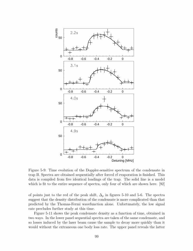
0

50

-0.8 -0.6 -0.4 -0.2 0co

unts

0

50

-0.8 -0.6 -0.4 -0.2 0

0

50

-0.8 -0.6 -0.4 -0.2 0

0

50

-0.8 -0.6 -0.4 -0.2 0 Detuning [MHz]

Figure 5-9: Time evolution of the Doppler-sensitive spectrum of the condensate intrap B. Spectra are obtained sequentially after forced rf evaporation is finished. Thisdata is compiled from five identical loadings of the trap. The solid line is a modelwhich is fit to the entire sequence of spectra, only four of which are shown here. [92]

of points just to the red of the peak shift, ∆p in figures 5-10 and 5-6. The spectrasuggest that the density distribution of the condensate is more complicated than thatpredicted by the Thomas-Fermi wavefunction alone. Unfortunately, the low signalrate precludes further study at this time.

Figure 5-11 shows the peak condensate density as a function of time, obtained intwo ways. In the lower panel sequential spectra are taken of the same condensate, andso losses induced by the laser beam cause the sample to decay more quickly than itwould without the extraneous one body loss rate. The upper panel reveals the latter

99

Figure 5-10: time evolution of Doppler-free spectrum of condensate in trap B. Thenoted time is measured from the end of the forced evaporative cooling cycle to themiddle of the sweep. Each spectrum is fit independently with a two parameter model:the peak density ∆p and an overall scaling factor S0; the background is estimatedindependently. The right side is not fit because of signal spillover from the veryintense DF normal line (not shown). This data is a compilation of sweeps from eachof five identical loadings of the trap.

situation. Here the sample is held for various intervals after forced rf evaporation isfinished, before laser probing is commenced. The sequence of spectra obtained is fit,and a peak condensate density at the beginning of the laser scan is obtained. Thisdensity is plotted in the figure. We see that the laser probe shortens the condensatelife by only a small factor. We also observe that in the absence of losses induced bythe laser, the condensate density decays by only a factor of 2 over 15 s (populationdecays by factor of 25/2 ≃ 6).

The number of atoms lost from the condensate through dipolar decay during this

100

Figure 5-11: Time evolution of peak density of the condensate in trap B. The lowerpanel shows the peak condensate density extracted from a sequence of DS spectra,some of which are shown in figure 5-9. The upper panel is the peak condensate mea-sured after waiting various times between the end of the forced evaporation cycle andthe beginning of the laser scans. This data demonstrates the lifetime of the conden-sate when the only loss mechanism is dipolar relaxation. The solid lines are from amodel of the heating and cooling processes in the normal gas and condensate. For thelower panel a one-body loss rate was introduced. The inset shows the calculated sam-ple temperature evolution in the absence of extraneous atom loss due to the presenceof the probe laser.

interval d = 15 s can be easily estimated by integrating equation 2.15:

Nc,lost =∫ d

0dt N2,c =

16

105

g

2!0θU

3/20

∫ d

0dt n7/2

p (t) (5.9)

101

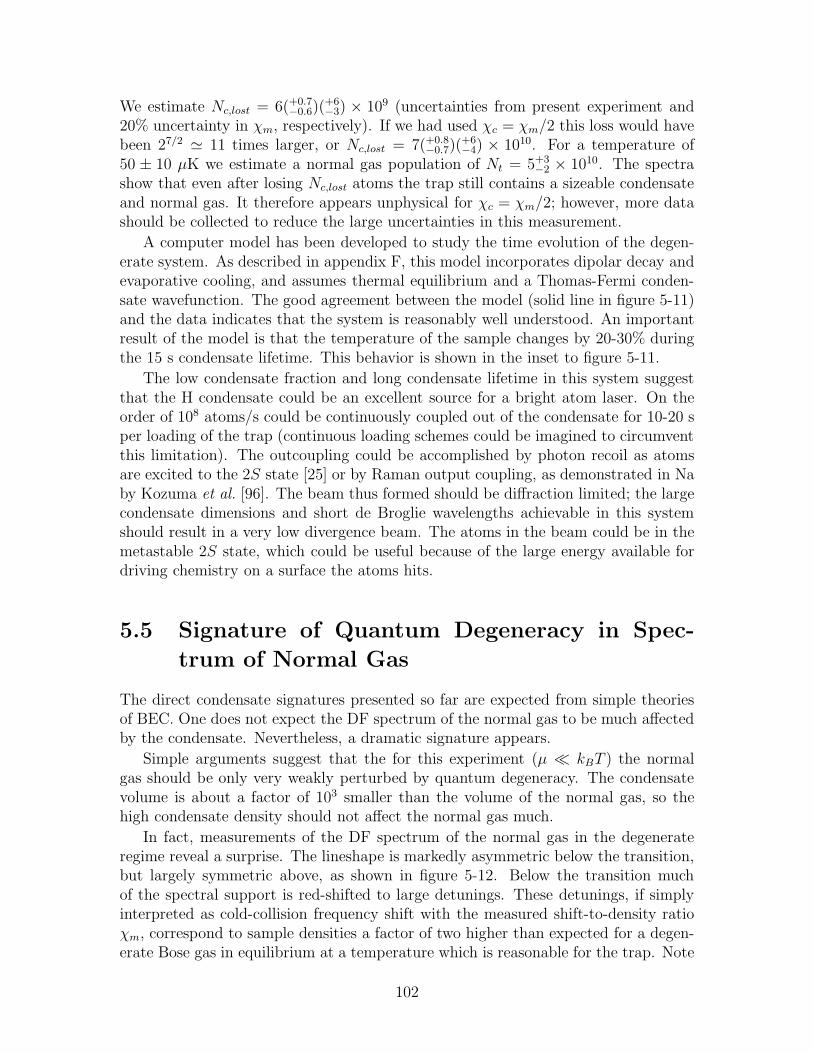
We estimate Nc,lost = 6(+0.7−0.6)(

+6−3) × 109 (uncertainties from present experiment and

20% uncertainty in χm, respectively). If we had used χc = χm/2 this loss would havebeen 27/2 ≃ 11 times larger, or Nc,lost = 7(+0.8

−0.7)(+6−4) × 1010. For a temperature of

50 ± 10 µK we estimate a normal gas population of Nt = 5+3−2 × 1010. The spectra

show that even after losing Nc,lost atoms the trap still contains a sizeable condensateand normal gas. It therefore appears unphysical for χc = χm/2; however, more datashould be collected to reduce the large uncertainties in this measurement.

A computer model has been developed to study the time evolution of the degen-erate system. As described in appendix F, this model incorporates dipolar decay andevaporative cooling, and assumes thermal equilibrium and a Thomas-Fermi conden-sate wavefunction. The good agreement between the model (solid line in figure 5-11)and the data indicates that the system is reasonably well understood. An importantresult of the model is that the temperature of the sample changes by 20-30% duringthe 15 s condensate lifetime. This behavior is shown in the inset to figure 5-11.

The low condensate fraction and long condensate lifetime in this system suggestthat the H condensate could be an excellent source for a bright atom laser. On theorder of 108 atoms/s could be continuously coupled out of the condensate for 10-20 sper loading of the trap (continuous loading schemes could be imagined to circumventthis limitation). The outcoupling could be accomplished by photon recoil as atomsare excited to the 2S state [25] or by Raman output coupling, as demonstrated in Naby Kozuma et al. [96]. The beam thus formed should be diffraction limited; the largecondensate dimensions and short de Broglie wavelengths achievable in this systemshould result in a very low divergence beam. The atoms in the beam could be in themetastable 2S state, which could be useful because of the large energy available fordriving chemistry on a surface the atoms hits.

5.5 Signature of Quantum Degeneracy in Spec-

trum of Normal Gas

The direct condensate signatures presented so far are expected from simple theoriesof BEC. One does not expect the DF spectrum of the normal gas to be much affectedby the condensate. Nevertheless, a dramatic signature appears.

Simple arguments suggest that the for this experiment (µ ≪ kBT ) the normalgas should be only very weakly perturbed by quantum degeneracy. The condensatevolume is about a factor of 103 smaller than the volume of the normal gas, so thehigh condensate density should not affect the normal gas much.

In fact, measurements of the DF spectrum of the normal gas in the degenerateregime reveal a surprise. The lineshape is markedly asymmetric below the transition,but largely symmetric above, as shown in figure 5-12. Below the transition muchof the spectral support is red-shifted to large detunings. These detunings, if simplyinterpreted as cold-collision frequency shift with the measured shift-to-density ratioχm, correspond to sample densities a factor of two higher than expected for a degen-erate Bose gas in equilibrium at a temperature which is reasonable for the trap. Note

102

Figure 5-12: Doppler-free spectra of normal gas showing asymmetry in quantumdegenerate regime. The spectra in the upper panel correspond to samples abovequantum degeneracy; those in the lower panel are for samples that are degenerate.The trap shapes are identical, and the trap depths are indicated. Note the differencein vertical scale. The lines connecting the points are a guide to the eye. The errorbars are statistical, and do not reflect systematic errors such as fluctuations in beamalignment and laser power.

that χm was measured in samples far from quantum degeneracy. If χ were larger bya factor of two for the part of the cloud in the bottom of the trap where the effectivechemical potential is small, then the asymmetric lineshape would make qualitativesense. The atoms in the highest density (red-shifted) part of the spectrum would tendto be shifted even further (because their χ is larger) than their low density counter-parts. However, no quantitative theory has been formulated predicting that χ shouldvary for the normal gas as quantum degeneracy is approached.

103

5.6 Density Shift for Excitation out of the Con-

densate and the Normal Gas

A thorough treatment of the relation between χc and χm has been undertaken byKillian [13]. He concludes that χc = χm/2 because exchange effects should be presentin the normal gas, but absent in a condensate. Here we discuss experimental evidencewhich suggests that perhaps χc = χm.

Time Evolution As explained in section 5.4, the condensate is observed to persistfor many seconds. Integration, over the lifetime of the condensate, of the rate ofatom loss through dipolar decay in the condensate is very sensitive to χc becausethe loss rate is proportional to n7/2

p ; a factor of two difference in χc translates to afactor of 11 change in the loss rate. If we take χc = χm/2 then the number of atomslost, Nc,lost from equation 5.9, is as large as the total original population of the trap!The estimate here would be flawed if the trap parameters (α, β, θ) applicable to thecondensate were somehow different from those for the thermal gas. This is unlikely,as noted in discussion of the trap shape in appendix G.

DS-DF Comparison Doppler-sensitive excitation results in excited atoms movingat the recoil velocity vrecoil ∼ 3 m/s. These motional states are very different from thelow energy motional states inhabited during Doppler-free excitation. Furthermore,the high velocity of the recoiling atoms implies that motional coherence betweenthe ground and excited states of the atom is very quickly lost during excitation,a situation conceivably different for DF excitation. Nevertheless, the condensatespectra obtained using the two different techniques are identical to within the (small)statistical uncertainty.

Spectroscopic Measurement of Condensate Fraction The condensate frac-tion measured spectroscopically agrees well with the fraction one computes from thepopulation in the condensate, assuming χc = χm. If χc = χm/2 then the calcu-lated condensate fraction is 25/2 ≃ 6 times larger than indicated by the spectroscopictechnique.

The possibility should be explored that χ = 2h(a2S−1S − a1S−1S)/m (instead of4h(a2S−1S−a1S−1S)/m) for excitation out of the thermal gas. Then it would be easy tounderstand why χc = χm. Furthermore, the asymmetric spectra presented in section5.5 could be understood if χ changed from the first to the second value in the normalgas near quantum degeneracy. If this were true all ambiguity would be relieved.Experiments designed to guarantee that the 1S and 2S atoms are distinguishablecould conceivably provide insight into this issue. This possibility is addressed insection 6.3.5.

The Bose condensates reported in this chapter open possibilities for many newexperiments. Some of these ideas are presented in the following chapter.

104

Chapter 6

Conclusion

6.1 Summary and Significance of this Work

We have created Bose-Einstein condensates of atomic hydrogen, culminating a longresearch effort. In the process we have confirmed that, as explained by Surkov et al.

[32], the reduced dimensionality of the evaporation process was the crippling factorin previous efforts to reach this goal in our lab [29] and in Amsterdam [30]. Ourcondensates, while huge compared to other condensates, are only a small fractionof the total trap population, a prediction by Hijmans et al. [45] for spin-polarizedhydrogen in equilibrium. We have this huge number of atoms in the trap because ofthe cryogenic loading technique we use, which can be scaled to arbitrarily large trapsizes (consistent with the scaling arguments in section 2.3.4). This cryogenic loadingmethod has been generalized for arbitrary paramagnetic atoms and molecules byDoyle and coworkers [97, 98, 99, 100], and therefore it should be possible to createbig condensates of arbitrary bosons. The high condensation flux we observe (109

atoms condensed per second for 10 s) should be useful in creating a bright atom laser.In addition, we have added another atom to the list of Bose-condensed species. Insection 2.3 we explored many differences between the hydrogen system and the alkalimetal gases that have been condensed so far. Finally, we have developed and appliedspectroscopy as a new probe of condensates.

6.2 Improvements to the Apparatus

The experiments described in this thesis were frustrated by several factors. Changesin the apparatus could allow us to investigate several new areas.

One of the most straightforward improvements is to reduce the stray electric fieldsin the cell. Large fields reduce the lifetime of the 2S atomic state by Stark quenching;the lifetime in a static electric field E (neglecting the natural lifetime) is [101]

τSQ =

(

475 V/cm

E

)2

1.6 ns. (6.1)

105

In the current cell, with its non-conducting walls, static charges reduce the 2S lifetimeto 0.1-1 ms, but in previous experiments in a metal cell [25] we have observed lifetimeson the order of the natural lifetime, τ0 = 120 ms. It should be possible to reduce strayfields by more than an order of magnitude by coating the inside of the plastic cell witha thin metallic film. Longer 2S lifetimes would allow us to address questions suchas how interactions with the condensate affect the 2S lifetime. Also, low stray fieldswould allow atoms ejected from the condensate in an atomic beam to travel manycentimeters toward the detector before decay (see section 6.3.3). Reduced stray fieldswould allow optical excitation to remain coherent for many milliseconds, allowinginteresting studies of the excitation process. The large stray fields increase indirectlythe background counts in our data: because of the short lifetime, fewer atoms canbe accumulated in the 2S level before the detection pulse, and so more detectionpulses must be used to accumulate the same signal. Each detection pulse increasesthe number of background counts. Reduction of stray fields would thus increase oursensitivity.

Another straightforward improvement is to reduce the heat load on the refrigeratorcaused by high power in the rf coils. The rf evaporation could then begin at highersample temperatures, and more efficient cooling would undoubtedly result. Moreatoms in the condensate would increase the signal rates, and more detailed studies ofthe condensate would be possible. The heat load created by the rf coils appears tonot be a consequence of the fields themselves, but rather of the system that conveysthe power to the coils. If the coils were thermally anchored to the 4.2 K 4He bath theheating of the refrigerator should be dramatically reduced.

Better knowledge of the trap shape and laser alignment could allow more detailedstudies of the influence of quantum degeneracy on the momentum distribution of thesample, as developed in section 6.3.2. As noted by Killian [13], better knowledge oftrap and laser geometry would also allow more accurate measurements of χ. We couldbetter understand the sizes of the condensates we produce (recall how in section 5.4the 20% error on χm translates into nearly a factor of two uncertainty in the numberof condensate atoms lost during the lifetime of the condensate). The evidence forχc = χm presented in section 5.6 could then be either bolstered or refuted, resultingin better understanding of the system.

The experiments probing the condensate, described in chapter 5, suffer from lowsignal rate. Straightforward improvements to the apparatus should allow at least afactor of 10 increase in detection solid angle, thus allowing studies at higher timeresolution to be feasible. Condensate formation and feeding could be studied in moredetail. The detection solid angle could be improved by moving the cold atoms into ashort trap formed by small currents in thin coils. This small trap could be surroundedby Lyman-α detectors.

6.3 Suggestions for Experiments

The success of the experiments described in this thesis has fertilized thinking aboutmany new experiments that could be done. In this section we discuss several of these

106

ideas.

6.3.1 Creating Bigger Bose Condensates

Nearly any experiment is easier with a larger condensate, and so here we discussstrategies for putting more atoms into a hydrogen condensate.

First, more atoms could be initially loaded into the trap. We do not currentlyunderstand the loading process in detail. Investigations are underway to explorepossibilities for loading more efficiently from the discharge. In addition to increasingthe loading efficiency, one could also simply increase the physical volume of the trapby making it longer and of larger diameter. One should be able to load a factor offour more atoms by scaling up the apparatus using available technology.

The overall phase space compression efficiency exponent for cooling from loadingconditions to BEC is γ = −1.5, which is small (see section A.2.3). Improvements tothe cooling efficiency could be made using two strategies. The first is to commencerf evaporation earlier in the cooling cycle. The second is to increase the ratio of goodcollisions to bad collisions. It is probable that the admixture of an alkali “moderator”atom “M” in the sample could dramatically increase the effective collision rate withoutsignificantly increasing the dipolar decay rate [51]. Presumably the cross-section forH-M collisions would be much greater than the anomalously low H-H cross-section.

Finally, improvements could be made to the cooling procedure that do not requireany changes to the apparatus. Instead of using the rf cooling paths shown in figure5-4, the sample could first be compressed at constant trap depth, the depth beingset by the highest rf frequency usable in the apparatus. Phase space compressionwould be accomplished at higher temperature, and thus more efficiently. After thiscompression the sample could be cooled to BEC at high density.

6.3.2 Probing the Velocity Distribution of the Normal Com-

ponent of a Degenerate Gas

In section 5.3.2 we described the influence of quantum degeneracy on the velocity dis-tribution of the normal gas. The expected spectrum is narrower and more cusp-shapedthan for a classical gas at the same temperature. Here we consider an experimentdesigned to compare these spectra.

In order to ensure that the two samples (classical and quantum) being probedhave the same temperature, we propose to use a single sample, but probe two partsof it. The inhomogeneous trapping potential serves to reduce the sample density(and thus the local chemical potential) in regions far from the deepest point in thetrap. Classical behavior can be observed in a gas containing a condensate when theprobe laser is translated a distance ρp ≫ kBT/α from the trap axis (for an IP trapwith T ≥ θ/kB). The beam diameter should be small compared to the translationdistance, a condition that is easy to fulfill in an open trap (small α).

The signal rate is dramatically reduced by the small densities far from the middleof the trap. In order to obtain the same signal rates as the present experiments(in which the high density central portion of the sample is probed), the detection

107

efficiency must be increased by the ratio of the densities, n(ρ = 0)/n(ρp). For trap Bin table 5.2, and for ρp = 3kBT/α = 160 µm, the required improvement in detectionefficiency is about

n(ρ = 0)

n(ρp)≃ g3/2(1)

g3/2(e−3)

Υ1/2(η, 0)

Υ1/2(η − 3,−3)≃ 102. (6.2)

Here we have used equation C.2 and figure C-1. A redesign of the apparatus for betteroptical access is required.

6.3.3 Creation of an Atom Laser

Atoms excited to the 2S state by co-propagating photons receive a momentum kickpr = 2h/λ where λ = 243 nm is the excitation wavelength. The atoms leave the exci-tation region with the recoil velocity vr = 3.28 m/s added vectorially to their initialvelocity. In the normal gas there is a wide distribution of velocities, so only a tinyfraction are Doppler-shifted into resonance for a given detuning. In the condensate,however, the velocity distribution is very narrow, and one might expect to interactoptically with all the condensate atoms at the same laser tuning. Atoms excitedout of the (coherent) condensate by a laser beam with a long coherence time shouldconstitute a coherent atomic beam. The divergence of this beam of atoms shouldbe diffraction limited by the size of the excitation region. Such a scheme has beendemonstrated by Kozuma et al. [96] using Raman pulses.

Unfortunately, several complications arise. First, the condensate spectrum isbroadened by the cold-collision frequency shifts arising from the high and inhomoge-neous condensate density. Since these shifts are much greater than the laser linewidth,the laser only interacts with a small fraction of the condensate for a given detuning.(One can imagine efficient methods of broadening the laser linewidth to match thecondensate linewidth [102], resulting in excitation of all the condensate atoms, butthis broadening would write decoherence onto the ejected atoms.) Since the opticalradiation only excites atoms from regions of a given density (corresponding to thedetuning), the excitation region can be quite small, and the divergence of the beamis enlarged. For example, atoms excited by a laser beam of linewidth 2 kHz thatis tuned to the peak condensate density will come from a region of diameter on theorder of ωexc = 1 µm. The resulting divergence angle is h/prπωexc = 4 × 10−2 [103].The situation is more complicated when the laser is detuned to interact with atomsin regions of intermediate density. Here the excitation occurs on a shell; interestingdiffraction effects should occur.

As the 2S atoms propagate with recoil velocity vr, the potential surface they ex-perience is strongly perturbed by the strong attractive mean field potential createdby the high condensate density. The depth of this potential for the peak condensatedensities listed in table 5.2 is on the order of 50 µK. The depth is small comparedto the 650 µK of recoil kinetic energy, so the atom has enough energy to leave thecondensate. However, the depth is much larger than the energy in the radial coor-dinates, µ/kB = 2 µK. One expects focusing effects as the recoiling atoms leave the

108

condensate.

The 1S-2S excitation process does not effect the hyperfine state of the atom; therecoiling atoms are still in the d-state, and are trapped. As the atoms move towardthe magnetic barrier that forms the end of the trap they slow down. Dephasing alsooccurs because the integrated action for slightly different atomic trajectories quicklybecomes quite different in the mountainous potential surface the atoms explore asthey leave the trapping region. In order to circumvent these problems of slowing anddephasing we propose to flatten the potential surface: we put the atoms in a magneticfield insensitive state by driving the d-a transition for the 2S atoms. The transitioncan be driven selectively for only the 2S atoms because the hyperfine splitting of the2S state is 23 = 8 times smaller than the 1S hyperfine splitting of 1420 MHz. Onemight be concerned that the rf field would drive d-c state transitions in the cold cloudof 1S atoms, and thus change the effective trap depth. This does not occur becausethe frequency is too large (178 MHz corresponds to a trap depth of 8.5 mK). Thea-state 2S atoms are free to fall out of the trapping region. In the current apparatusthe atoms can fall a height h = 20 cm before hitting a window. This should take a

time τfall = (−vr/g)(1 −√

1 + 2gh/v2r) = 56 ms for atoms with downward directed

recoil velocity, and τfall = (vr/g)(1 +√

1 + 2gh/v2r) = 790 ms for those with upward

directed recoil velocity. Here g is the acceleration of gravity. We do not expect todetect the atoms launched upward because the natural lifetime (120 ms) is too short,and because, in the current apparatus, the atoms will hit a surface before reachingthe peak of their 55 cm high trajectory.

Detection of the atomic beam could be accomplished by quenching the atomswith an applied electric field pulse when the atoms are at the bottom of the cellnear the detector. To estimate the signal size, we compare to the signal obtainedwhen the atoms are not allowed to move very far before detection, the experimentalprocedure for figure 5-5. We expect a reduction in the number of fluorescing atomsby e−τfall/τ0 ≃ 0.63 because of decay during the transit time τfall. We expect a factorof two further reduction because only 1/2 the atoms have downward-directed recoilvelocity. We expect an increase in signal because the detection solid angle is greaternear the bottom of the cell. With the current cell design we should be able to achievea factor of seven increase in detection efficiency, but with straightforward extensionsof the cell closer to the detector this factor could be another factor of ten larger.Neglecting this improvement, we expect the atoms in the atomic beam to yield aboutthe same signal size as observed in figure 5-5. The experiment is thus feasible in a cellidentical to the current one, but a conductive coating to reduce stray electric fields isessential.

In addition to observing an atomic beam ejected from the sample, another in-teresting experiment would be a study of collisional quenching of the 2S atoms asthey move through the high density condensate. One might expect collisional de-excitation to occur on a time scale comparable to the characteristic collision time:τcol = 1/npσ2S−1Svrecoil ≃ 700 µs. A brief study indicated no collisional quenchingon the sub-millisecond time scale, but the study should be repeated for longer times.Reduction of the stray fields would allow this.

109

6.3.4 Measuring the Condensate Density through Dipolar

Decay

In the experiments described in chapter 5 the condensate density was measured spec-troscopically, but confusion arises around a factor of two in the conversion constant χcthat relates frequency shift to sample density. We propose an independent measureof condensate density which should resolve the ambiguity. The proposed measure-ment exploits two-body dipolar decay, which proceeds at a well known rate in thecondensate [44]. If the condensate density distribution is well approximated by theThomas-Fermi profile in equation 2.13, then the characteristic loss rate is given byequation 2.15. Using equation 2.14 we find that the peak shift (frequency shift ofmaximally shifted part of the spectrum) should decay in time as

∆p(t) =∆p,0

1 + 4g∆p,0

35χct

(6.3)

where ∆p,0 is the initial peak shift. The only free parameters used to fit this equationto measured data would be ∆p,0 and χc. The factor of two ambiguity in χc should beeasy to resolve. If the Thomas-Fermi density distribution is a poor approximation,then the factor 4/35 should be different. The quality of the fit of the Thomas-Fermi lineshape to the data in figures 5-5, 5-6, 5-9, and 5-10 indicates that thisapproximation is reasonable.

To measure the condensate decay time cleanly, we require that the condensate isnot being replenished by the normal gas. The most straightforward way to accomplishthis is a complete removal of the normal gas by rf ejection. The trap depth would bequickly swept down to the edge of the condensate, using high rf power to efficientlyoutcouple all the normal atoms. DF or DS spectroscopy of the condensate would thenprobe the time evolution of the peak shift, ∆p(t).

Since the lifetime of the condensate would be short, there would not be muchsignal accumulation time. The detection efficiency in the current apparatus is toolow, but a factor of six improvement should make this experiment feasible (a factor ofsix can be obtained by replacing the Lyman-α filter over the MCP with a window).Currently, sufficient signal can be obtained by summing 0.8 s sweeps from severalidentically prepared samples. A factor of six improvement would allow the sweeps tobe shortened to 0.13 s, short compared to the decay time 35χc/4g∆p,0 ≃ 1 s expectedfor χc = χm/2 and ∆p,0 ∼ 600 kHz.

6.3.5 Exchange Effects in Cold-Collision Frequency Shift

In section 5.6 we proposed that perhaps χc = χm, which would make sense if χm didnot include exchange effects for some reason. This could be tested by measuring thecold-collision frequency shift in the classical regime for atoms that are known to bedistinguishable. To ensure distinguishability, the atoms could be put into differenthyperfine states, c and d. A c-state atom interacting with a d-state atom shouldfollow an interaction potential that is very similar to the identical particle case, but

110

the mean-field interaction energy would be smaller by a factor of two because theatoms are distinguishable and exchange effects are absent. One expects two peaksin the DF spectrum: one from collisions between identical particles, which is shiftedtwice as much as the other, which is from collisions between distinguishable particles.If the observed spectrum contains only a single peak, then we conclude that the atomsare distinguishable in all collision processes. In that case we expect χc = χm.

We propose to do this experiment in a very deep trap (ǫt/kB ≫ (µB/kB)506 G =34 mK) so that the c-state atoms will be confined (see figure 1-1). We propose touse a sample typical of what exists immediately after loading the trap (T = 40 mK,n0 = 2 × 1013 cm−3). If half the atoms are transferred from the d to the c state, theexpected decay time of the c-state atoms is τ ≃ 2 s. The dominant terms in the lossrate are Gcc→aa = 1.4 × 10−13, Gcc→bd = 7× 10−14, and Gcc→ac = 6 × 10−14 cm3/s forfields around 600 G [104], which corresponds to the thermal energy. We must measurethe DF spectrum quickly compared to this time τ to observe how the spectrumchanges.

Time-of-flight broadening would be significant in this spectrum, on the 40 kHzlevel for the current laser beam waist (100 µm diameter). This is large compared to theexpected cold-collision frequency shifts of 2 and 4 kHz. To reduce the broadening, thebeam diameter could be expanded by a factor of ten. The excitation rate (proportionalto the square of the radiation intensity) would drop by 104, but the interaction volumewould increase by 102 (the sample diameter is larger than the beam diameter). Thelinewidth would narrow by a factor of ten because of the increased interaction time,and so the overall signal rate would drop by only a factor of ten. Samples canbe created every two minutes and systematics are easy to control, so it would bestraightforward to accumulate signal.

6.3.6 Measuring a1S−1S

The ground state s-wave scattering length has been calculated to the level of 10−2

[40], but has not been measured nearly as well. One could use the interaction energyU0np = 4πh2anp/m in the condensate to measure a, given the peak density np. Wepropose to measure the chemical potential µ directly in an experiment similar to themeasurement of χc in section 6.3.4. Using µ = U0np we obtain a = µm/4πh2np. Toget µ we measure the difference between the potential energies at the center (θ) andedge (εe) of the condensate. We measure θ by sweeping the rf frequency upward untilatoms begin to fall out of the trap, as described in section 4.2.4. We measure εe ina series of measurements of the sample density; the normal atoms are removed bysweeping the rf frequency down to some ending frequency fend, which is varied. Forfend slightly larger than εe/h the density measurements should give identical results.But for fend < εe/h the condensate is depleted, and the measured density decreases.

A measurement of a to the 10% level seems feasible. Consider trap B and a peakcondensate density np = 3 × 1015 cm−3. The bias field θ must not drift more than1 mG between measurement of θ and εe; this stability should be possible. To measureεe we vary fend and look for changes in the maximum frequency shift, as describedabove. Since the maximum frequency shift scales linearly with the chemical potential,

111

we must measure ∆p,0 to better than 10%. This should be possible with the factor ofsix detection efficiency improvement outlined above. Many spectra would be obtainedas the condensate decays, and so a group of many data points would be fit to the twoparameters in equation 6.3. Precision of 10% seems feasible.

6.3.7 Dynamics of 2S atoms in 1S condensate

As described in section 5.3.1 and in the thesis of Killian [13], condensate atoms ex-cited to the 2S state are confined radially by the deep interaction potential createdby the large condensate density. The motional eigenstates in the 2S potential arerather different from the 1S eigenfunction, the condensate wavefunction. We there-fore expect the 2S atoms to exist in superpositions of several of these excited stateeigenfunctions, and to thus oscillate across the condensate.

The initial position of the 2S atoms is tuned by the detuning of the excitation ra-diation field. The position after some delay time τ could be measured using Balmer-αabsorption imaging. One expects breathing modes. Coherence effects in the excita-tion process could be explored with this technique.

6.4 Outlook

The studies of Bose condensed hydrogen presented here constitute simply the appe-tizer in the feast of experiments to be carried out. Once ambiguities about χc arestraightened out and the fascinating asymmetric lines in section 5.5 are understood,the creation of the high-flux coherent atomic seems to be the next step. The beautifulatom laser experiments of Mewes et al. [105], Kozuma et al. [96], and Anderson andKasevich [11] should provide solid stepping stones.

112

Appendix A

Theory of Trapped Classical Gas

In this appendix we present the statistical mechanical treatment of a trapped idealgas, consider decay of the sample through relaxation of the spin-polarization, andcalculate the effects of evaporation. The appendix exists to familiarize the readerwith concepts and scaling laws useful for hydrogen trapping and cooling experiments.Simple relations describe samples trapped in deep potentials. Here we address theeffects of the finite trap depth, following the work of Luiten et al. [26]. We find thatthe truncation corrections are only important for shallow traps.

A.1 Ideal Gas

We begin our discussion by describing a trapped ideal gas in the classical regime.“Trapped” implies confinement by an inhomogeneous potential with a depth signifi-cantly greater than the characteristic energy of the gas particles. “Ideal” means thatcollisions among the atoms, although crucial for maintaining thermal equilibrium, arenot included in the Hamiltonian. The interaction energy for the densities studied inthis thesis will turn out to be very small compared to the thermal energy, except inthe case of when a condensate, as described in section 2.2.2. “Classical” means thatthe gas is far from quantum degeneracy, and the Maxwell-Boltzmann distributionadequately describes the correct quantum distribution. These approximations areappropriate for the trapped hydrogen gas studied in this thesis as it is cooled fromthe initial temperature of about 40 mK to near the onset of quantum degeneracyaround 50 µK.

In sections A.1.1 and A.1.2 we describe the occupation function for the gas and thedensity of states functions for traps of experimental interest. In section A.1.3 theseconcepts are employed to calculate various thermodynamic properties. In sectionA.1.4 we consider trap losses arising from decay of the spin-polarization of the trappedgas. Collisions and evaporative cooling are the topics of section A.2.

113

A.1.1 Occupation Function

We assume that the gas is well described by the Maxwell-Boltzmann distribution,except that the energy distribution is truncated at some trap depth energy ǫt. Thegas is said to be quasi-thermal. This is a reasonable assumption if two conditionshold [26]. First, the elastic collision rate must be high enough to redistribute particleenergies quickly compared to the rate at which processes occur which would take thegas out of equilibrium, such as changes in the trap shape or depth. This is calledthe “sufficient ergodicity” condition. (Elastic collisions are discussed in section A.2below.) Second, particles with energies greater than the trap depth must be removedpromptly compared to the rate at which they are promoted to the energetic states.Situations in which this condition is not satisfied have been discussed in section 2.1.

The phase space occupation function, f(ǫ), is the number of particles per unitvolume of phase space in a region of phase space with total energy ǫ = H(p, r). (His the Hamiltonian of the particle). We postulate an occupation function f(ǫ) that isthe Boltzmann factor [33] below the trap depth, and zero above:

f(ǫ) =

n0Λ3e−ǫ/kBT ; ǫ ≤ ǫt

0 ; ǫ > ǫt(A.1)

where Λ ≡ h/√

2πmkBT is the thermal de Broglie wavelength and n0 is a referencedensity; the normalization is the total number of trapped atoms. Evidence support-ing this postulate was obtained by numerical integration of the Boltzmann transportequation [26]. The occupation function of a simulated gas, described initially byf(ǫ) =const. below threshold ǫt and zero above, was observed to transform to theBoltzmann form in equation A.1 in a few characteristic collision times. The trappedgas is described by two parameters, T and n0, which correspond to sample temper-ature and maximum sample density in an infinitely deep trap [26]. For finite trapdepths, temperature is poorly defined because the distribution is truncated, and n0

is larger than the actual maximum sample density, as discussed in section 9.

A.1.2 Density of States

A useful concept is the density of states, the volume of parameter space correspondingto the fulfillment of some condition. We use two density of states functions. The“total energy density of states” function, ρ(ǫ), is the differential volume of phasespace corresponding to a total particle energy ǫ. (The number of particles N(ǫ)dǫwithin an energy dǫ of ǫ is the occupation per unit volume multiplied by the volume,N(ǫ)dǫ = f(ǫ)ρ(ǫ)dǫ.) The “potential energy density of states” function, (ε), is thedifferential volume of real space with potential energy ε. In this thesis ε will alwaysdenote a potential energy, and ǫ will always denote a total energy. Likewise, (ε) willalways be a potential energy density of states, and ρ(ǫ) will always be a total energydensity of states.

114

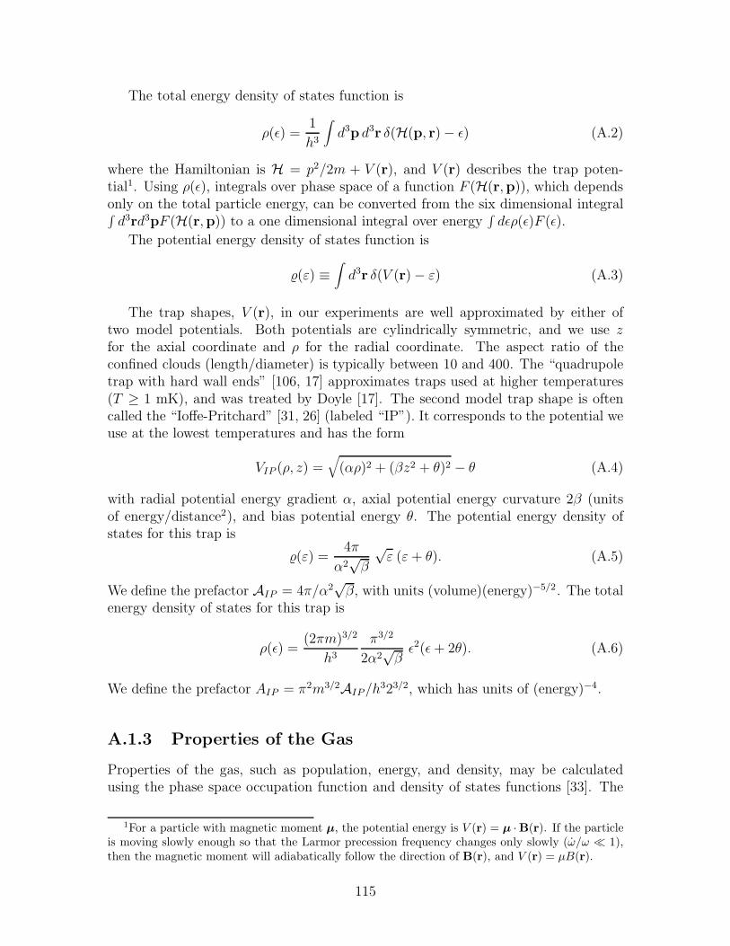
The total energy density of states function is

ρ(ǫ) =1

h3

∫

d3p d3r δ(H(p, r) − ǫ) (A.2)

where the Hamiltonian is H = p2/2m + V (r), and V (r) describes the trap poten-tial1. Using ρ(ǫ), integrals over phase space of a function F (H(r,p)), which dependsonly on the total particle energy, can be converted from the six dimensional integral∫

d3rd3pF (H(r,p)) to a one dimensional integral over energy∫

dǫρ(ǫ)F (ǫ).

The potential energy density of states function is

(ε) ≡∫

d3r δ(V (r) − ε) (A.3)

The trap shapes, V (r), in our experiments are well approximated by either oftwo model potentials. Both potentials are cylindrically symmetric, and we use zfor the axial coordinate and ρ for the radial coordinate. The aspect ratio of theconfined clouds (length/diameter) is typically between 10 and 400. The “quadrupoletrap with hard wall ends” [106, 17] approximates traps used at higher temperatures(T ≥ 1 mK), and was treated by Doyle [17]. The second model trap shape is oftencalled the “Ioffe-Pritchard” [31, 26] (labeled “IP”). It corresponds to the potential weuse at the lowest temperatures and has the form

VIP (ρ, z) =√

(αρ)2 + (βz2 + θ)2 − θ (A.4)

with radial potential energy gradient α, axial potential energy curvature 2β (unitsof energy/distance2), and bias potential energy θ. The potential energy density ofstates for this trap is

(ε) =4π

α2√β

√ε (ε+ θ). (A.5)

We define the prefactor AIP = 4π/α2√β, with units (volume)(energy)−5/2. The total

energy density of states for this trap is

ρ(ǫ) =(2πm)3/2

h3

π3/2

2α2√βǫ2(ǫ+ 2θ). (A.6)

We define the prefactor AIP = π2m3/2AIP/h323/2, which has units of (energy)−4.

A.1.3 Properties of the Gas

Properties of the gas, such as population, energy, and density, may be calculatedusing the phase space occupation function and density of states functions [33]. The

1For a particle with magnetic moment µ, the potential energy is V (r) = µ ·B(r). If the particleis moving slowly enough so that the Larmor precession frequency changes only slowly (ω/ω ≪ 1),then the magnetic moment will adiabatically follow the direction of B(r), and V (r) = µB(r).

115

number of trapped atoms, N , is

N =∫ ǫt

0dǫ f(ǫ)ρ(ǫ)

= n0Λ3Z (A.7)

where the single particle partition function is

Z =∫ ǫt

0dǫ ρ(ǫ) exp(−ǫ/kBT ) (A.8)

The N -particle partition function for a non-interacting classical gas is ZN = ZN/N !.

For a power law density of states given as ρ(ǫ) = ρ0 ǫδ+3/2 we obtain

Z = Z∞P (δ + 5/2, η) (A.9)

where η ≡ ǫt/kBT is a dimensionless measure of the trap depth (typically 4 < η < 10)and

Z∞ ≡ ρ0(kBT )δ+5/2Γ(δ + 5/2) (A.10)

is the partition function for an infinitely deep trap. The truncation correction factorP (q, η) is defined in equation A.12.

The partition function for the IP potential is2

ZIP =(kBT )5/23π3/2

Λ3α2√β

(

P (4, η) +2φ

3P (3, η)

)

(A.11)

where φ ≡ θ/kBT is a dimensionless measure of the trap bias energy and η ≡ ǫt/kBT isa dimensionless measure of the trap depth. We have introduced the function P (q, η),which is a correction factor for the finite trap depth [26]. It is related to the incompletegamma function Γ(q, η) ≡ ∫∞

η tq−1e−tdt by

P (q, η) ≡ 1

Γ(q)

∫ η

0tq−1e−tdt

=Γ(q) − Γ(q, η)

Γ(q)(A.12)

For large η the correction is negligible, and P (q, η) = 1. The behavior of P (q, η) isshown in figure A-1 for various values of q. The parameter q describes the energyexponents appearing in the trapping potential. As stated in equation A.11, the valuesq = 3 and q = 4 are of interest for the IP trap. Note that for η ≥ 7 there is onlya small deviation from the infinitely deep trap (corresponding to η → ∞) for theexponents δ of interest in this thesis.

2For this and many other non-trivial integrals we use the computer program for symbolic math-ematics called Mathematica.

116

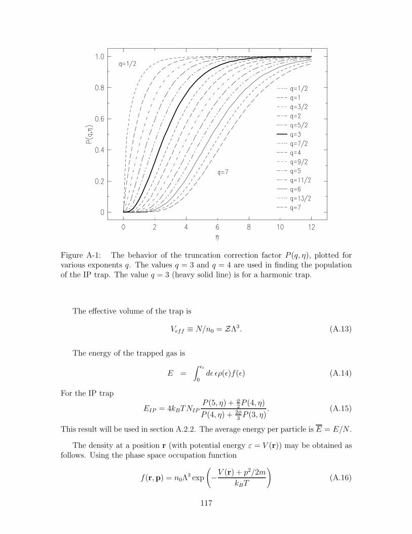
Figure A-1: The behavior of the truncation correction factor P (q, η), plotted forvarious exponents q. The values q = 3 and q = 4 are used in finding the populationof the IP trap. The value q = 3 (heavy solid line) is for a harmonic trap.

The effective volume of the trap is

Veff ≡ N/n0 = ZΛ3. (A.13)

The energy of the trapped gas is

E =∫ ǫt

0dǫ ǫρ(ǫ)f(ǫ) (A.14)

For the IP trap

EIP = 4kBTNIP

P (5, η) + φ2P (4, η)

P (4, η) + 2φ3P (3, η)

. (A.15)

This result will be used in section A.2.2. The average energy per particle is E = E/N .

The density at a position r (with potential energy ε = V (r)) may be obtained asfollows. Using the phase space occupation function

f(r,p) = n0Λ3 exp

(

−V (r) + p2/2m

kBT

)

(A.16)

117

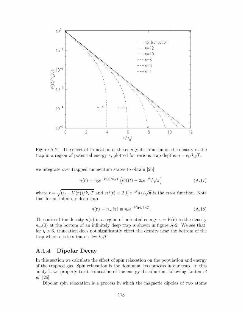
Figure A-2: The effect of truncation of the energy distribution on the density in thetrap in a region of potential energy ε, plotted for various trap depths η = ǫt/kBT .

we integrate over trapped momentum states to obtain [26]

n(r) = n0e−V (r)/kBT

(

erf(t) − 2te−t2

/√π)

(A.17)

where t =√

(ǫt − V (r))/kBT and erf(t) ≡ 2∫ t0 e

−s2ds/√π is the error function. Note

that for an infinitely deep trap

n(r) = n∞(r) ≡ n0e−V (r)/kBT . (A.18)

The ratio of the density n(r) in a region of potential energy ε = V (r) to the densityn∞(0) at the bottom of an infinitely deep trap is shown in figure A-2. We see that,for η > 6, truncation does not significantly effect the density near the bottom of thetrap where ǫ is less than a few kBT .

A.1.4 Dipolar Decay

In this section we calculate the effect of spin relaxation on the population and energyof the trapped gas. Spin relaxation is the dominant loss process in our trap. In thisanalysis we properly treat truncation of the energy distribution, following Luiten et

al. [26].Dipolar spin relaxation is a process in which the magnetic dipoles of two atoms

118

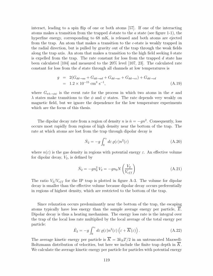
interact, leading to a spin flip of one or both atoms [57]. If one of the interactingatoms makes a transition from the trapped d-state to the a state (see figure 1-1), thehyperfine energy, corresponding to 68 mK, is released and both atoms are ejectedfrom the trap. An atom that makes a transition to the c-state is weakly trapped inthe radial direction, but is pulled by gravity out of the trap through the weak fieldsalong the trap axis. An atom that makes a transition to the high field seeking b stateis expelled from the trap. The rate constant for loss from the trapped d state hasbeen calculated [104] and measured to the 20% level [107, 23]. The calculated rateconstant for loss from the d state through all channels at low temperatures is

g = 2(Gdd→aa +Gdd→ad +Gdd→ac +Gdd→cc) +Gdd→cd

= 1.2 × 10−15 cm3 s−1, (A.19)

where Gσλ→φψ is the event rate for the process in which two atoms in the σ andλ states make transitions to the φ and ψ states. The rate depends very weakly onmagnetic field, but we ignore the dependence for the low temperature experimentswhich are the focus of this thesis.

The dipolar decay rate from a region of density n is n = −gn2. Consequently, lossoccurs most rapidly from regions of high density near the bottom of the trap. Therate at which atoms are lost from the trap through dipolar decay is

N2 = −g∫ ǫt

0dε (ε)n2(ε) (A.20)

where n(ε) is the gas density in regions with potential energy ε. An effective volumefor dipolar decay, V2, is defined by

N2 = −gn20 V2 = −gn0N

(

V2

Veff

)

(A.21)

The ratio V2/Veff for the IP trap is plotted in figure A-3. The volume for dipolardecay is smaller than the effective volume because dipolar decay occurs preferentiallyin regions of highest density, which are restricted to the bottom of the trap.

Since relaxation occurs predominantly near the bottom of the trap, the escapingatoms typically have less energy than the sample average energy per particle, E.Dipolar decay is thus a heating mechanism. The energy loss rate is the integral overthe trap of the local loss rate multiplied by the local average of the total energy perparticle:

E2 = −g∫ ǫt

0dε (ε)n2(ε)

(

ε+K(ε))

. (A.22)

The average kinetic energy per particle is K = 3kBT/2 in an untruncated Maxwell-Boltzmann distribution of velocities, but here we include the finite trap depth in K.We calculate the average kinetic energy per particle for particles with potential energy

119

Figure A-3: The volume for dipolar decay compared to the effective volume, plottedfor various bias fields φ = θ/kBT . The difference between large φ (harmonic) andsmall φ (linear radial confinement) arises because in the harmonic trap the densitydistribution is flatter in the middle. For a box potential the density distribution iscompletely flat, and the two volumes are identical.

ε in a trap of depth ǫt:

K(ε) =

∫√

2m(ǫt−ε)

0d3p

p2

2me−p

2/2mkBT

∫√

2m(ǫt−ε)

0d3p e−p

2/2mkBT

= kBT6t+ 4t3 − 3s

4t− 2s(A.23)

where s =√πerf(t) exp(t2) and t =

√

(ǫt − ε)/kBT . Figure A-4 shows the behavior

of K. The average energy carried away per atom is C2kBT ≡ E2/N2. This is plottedin figure A-5 for the IP trap, for various values of φ. We see that for η ≥ 6 we canreasonably ignore truncation effects.

120

Figure A-4: The mean kinetic energy of atoms in a region of given potential energy,plotted for samples in traps of various depths. The trap appears shallower for atomsat higher potential energies.

A.2 Collisions and Evaporative Cooling

So far we have not addressed elastic collisions, but they play a crucial role in thedynamics of the trapped gas. In this section we examine we examine the role ofcollisions in maintaining thermal equilibrium and in evaporatively cooling the sample.We calculate the equilibrium temperature of the gas. And we conclude the sectionwith a discussion of an impediment to efficient evaporative cooling, the impedimentthat prevented the creation of BEC in hydrogen before this work.

Only low energy collisions occur in our cold samples, so the elastic scatteringprocess is described by quantum mechanical s-wave scattering theory3 [108, 27]. Theresult of this theory is that elastic interactions are parameterized by a single quantity,the s-wave scattering length a. The cross section for collisions between identical

particles is σ = 8πa2. In a gas of density n and mean particle speed v =√

8kBT/πm,

the collision rate is Γcol(n) = nσv√

2. The collision rate determines the time scale forenergy redistribution in the gas.

A sample in a trap of finite depth is never in complete equilibrium since collisionsconstantly tend to populate that portion of the equilibrium energy distribution whichlies above the trap depth. The removal of these energetic atoms is called evaporation.

3s-wave scattering is allowed for identical bosons, but is prohibited for identical fermions

121

Figure A-5: The average total energy per atom that is lost from a Ioffe-Pritchardtrap through dipolar relaxation, in units of kBT . The parameter φ ≡ θ/kBT is thestrength of the bias field, and η ≡ ǫt/kBT is the trap depth. We see that we canignore truncation effects for η ≥ 6. For the harmonic trap (large φ) the particles haveless potential energy because the potential is quadratic; in the linear radial potential(small φ) there is more potential energy per particle.

Its use as a cooling mechanism for a trapped atomic gas was first proposed by Hess[106] and was first demonstrated in the MIT spin-polarized hydrogen group [109].Evaporation occurs when a collision of two atoms transfers enough energy to oneatom that it may escape the trap. This atom leaves the trap with an energy ǫ > ǫt,much greater than the average energy per atom in the sample, E. The averageenergy per remaining particle is lower, and after rethermalization of the trapped gas,the temperature is lower. Cooling has occurred. Note that rethermalization is givena headstart by the preferential evaporation of atoms from the upper end of the energydistribution, closer in energy to the trap depth, ǫt, as described in appendix B.

A.2.1 Evaporative Cooling Rate

The evaporative cooling rate for a sample described by a truncated Boltzmann oc-cupation function has been calculated by Luiten et al. [26] using the Boltzmanntransport equation. We quote their results here.

122

Figure A-6: The quantity Vevap/Veff for an IP trap as a function of η, plotted forvarious bias fields φ = θ/kBT . The inset shows Vevape

η, which becomes linear in η forlarge η. This linear relation is useful when estimating evaporation rates.

The particle loss rate due to evaporation is

Nevap = −n20 σ v Vevap = −N Γcol(n0)√

2

VevapVeff

, (A.24)

a product of the total population, a characteristic collision rate, and the fraction ofcollisions which produce an atom with enough energy to escape. The ratio Vevap/Vefffor an IP trap is plotted in figure A-6 for various φ = θ/kBT (we use equation 43afrom [26]).

The energy loss rate due to evaporation is given by equation 40 in [26]:

Eevap = NevapkBT η + 1 −Xevap/Vevap (A.25)

where Xevap is a truncation correction factor. Figure A-7 shows the behavior ofXevap/Vevap for the IP trap (we use equation 43b from [26]). For large η, the quantityin curly braces in equation A.25 is nearly η + 1.

A.2.2 Equilibrium Temperature

The temperature of the trapped gas is set by a competition between heating dueto dipolar relaxation and cooling due to evaporation. The sample is in dynamic

123

Figure A-7: The quantity Xevap/Vevap for an IP trap as a function of η = ǫt/kBT ,plotted for various bias fields φ = θ/kBT . The volume Xevap is a small contributionto the evaporation volumes for η ≥ 6

equilibrium when the temperature is no longer changing, meaning that the averageenergy per particle is stationary. Setting d(E/N)/dt = 0 dictates that

E

N=E

N=Eevap + E2

Nevap + N2

(A.26)

If the temperature drops below equilibrium, the evaporation rate drops exponentially.In addition, the effective volume decreases, the density increases, and the heating ratedue to dipolar decay increases. On the other hand, if the temperature increases aboveequilibrium, the heating rate decreases and the evaporative cooling rate increases. Adynamic equilibrium is thus maintained.

The equilibrium temperature is found by numerically solving equation A.26. Fornotational simplicity we define the factor B which indicates whether the IP trap isprimarily linear or harmonic in the radial direction,

B(η, φ) ≡ P (5, η) + φP (4, η)/2

P (4, η) + 2φP (3, η)/3. (A.27)

124

Figure A-8: Graphical solution of the heating/cooling balance equation, plotted fortraps of various depths ǫt. The bias energy is θ/kB = 34 µK. The heavy lines are theright hand side (rhs) of equation A.28. The light lines are the left hand side. Thesolid dots indicate the equilibrium temperature for the various trap depths. At lowertemperatures the equilibrium η is smaller, indicating less efficient evaporation.

Then equation A.26 may be written

Nevap

N2

=4B(η, φ) − C2

η + 1 + Xevap

Vevap− 4B(η, φ)

. (A.28)

The left and right hand sides are plotted in figure A-8 for typical trap depths and abias field θ/kB = 34 µK. The equilibrium η is larger at higher temperatures becausethe mean particle speed, and thus collision rate, is higher. The higher η at highertemperatures indicates that evaporative cooling is more efficient there; fewer atomsare expended in the battle against heating caused by dipolar decay.

A.2.3 Forced Evaporative Cooling

The analysis above indicates that, for a given trap depth, a minimum temperaturewill be achieved which is set by the competition between heating and cooling. Inorder to cool the sample further the trap depth must be reduced. A comprehensivereview by Ketterle and van Druten [56] of forced evaporation analyses the process

125

in detail. For the experiments described in this thesis the trap depth is reduced byeither lowering the magnetic confinement field at one end of the trap, or by reducingthe frequency of an RF magnetic field that selectively removes the most energeticatoms. This second method is the focus of chapter 3.

A computer model (described in appendix D) has been used to evolve in time thetotal energy and total number of particles in the sample as it is cooled. Temperatureand density are calculated along the way. The effects of changing the trap depthand changing the functional form of the trapping potential have been included. Thismodel agrees well with experiments.

The rate at which the temperature of the gas can be changed is an important pa-rameter. Luiten et al. [26] have shown that a classical gas with an energy distributionfar from equilibrium will reasonably approximate a Maxwell-Boltzmann distributionafter about three collision times. One therefore expects fluctuations of the energydistribution to dissipate on this time scale. To maintain quasi-equilibrium the trapdepth and the trapping potential should thus be changed slowly compared to thiscollision time.

Since trapped atoms are a scarce commodity, a figure of merit for a cooling processis the amount of phase space compression achieved per atom lost. Far from quantumdegeneracy the phase space density is the number of atoms per cubic thermal deBroglie wavelength, D ≡ nΛ3. A useful measure of the cooling efficiency is the coolingexponent [56], which is the differential fractional change in phase space density perdifferential fractional change in population,

γ ≡ d logD

d logN. (A.29)

A large, negative value indicates that the phase space density increases by a largefactor for a decrease in population by only a small factor. Cooling exponents as largeas γ = −3 have been observed [110].

In cooling clouds of alkali metal atoms, a process called “runaway evaporation” isobserved, in which cooling of the sample leads to an increase in sample density becausethe atoms are more localized in the bottom of the trap. In turn, the increased densityleads to an increased collision rate and faster evaporation. The cooling accelerates,a desirable phenomena because the number of atoms lost through background gascollisions during the time used to cool the sample is reduced when the cooling timeis shorter. The conditions required for runaway evaporation are carefully explainedby Ketterle et al. [56]. Runaway evaporation does not occur in clouds of trappedhydrogen because the dominant loss rate, due to dipolar relaxation, increases withincreasing density with the same exponent as the evaporation rate. The ratio of theevaporation loss rate (“good” losses) to the dipolar decay loss rate (“bad” losses),

Nevap

N2

=σvVevapgV2

∼ 50e−η(η − 4.5)

√

T

1 µK, (A.30)

is independent of density, depending only on√T for a given η. The effective volumes

126

for dipolar decay and evaporation used in equation A.30 are for φ ∼ 1 and η > 7.From this equation we see that evaporation is more efficient at higher temperatures,as noted above.

127

128

Appendix B

Fraction of Collisions Which

Produce an Energetic Atom

In a collision between two atoms with a medium energy, what is the probability ofcreating an “energetic atom”, i.e. an atom with enough energy to escape the trap?Consider a collision between two distinguishable particles of identical mass m andinitial momenta p1 and p2. After the collision the momenta are labeled q1 and q2.The total and relative momenta are P = (p1 + p2) and p = p1 − p2, and similarlyfor Q and q.

Conservation of momentum leads to the equation P = Q. We orient the axes ofthe coordinate system so that Q = Qz and we work in spherical coordinates. Thetotal energy is

E0 = (P 2 + p2)/4m. (B.1)

Conservation of energy demands that p2 = q2. We thus have four equations and sixunknowns, leaving two undetermined coordinates, which will be labeled θ and φ inthe description of

q = q (x cosφ+ y sinφ) sin θ + z cos θ .

After aligning the coordinate system we see that the there are two conserved scalarquantites, P = Q and p = q. We can compute the fraction of this allowable phasespace corresponding to various conditions by assuming that, in a collision, θ and φmay take any value with equal probability. We define the function f(θ, φ) dΩ as thevolume of phase space within a differential solid angle dΩ of the given angles. Sincethe collisions are postulated to be independent of angle, we take f(θ, φ) = f0 = 1/4π.

In the calculations to follow we scale the energies to the trap depth, Et. We usethe dimensionless variables a ≡ q/

√4Etm and b = Q/

√4Etm. The total energy is

then E0 = Et(a2 + b2).

We first find the fraction of phase space corresponding to one atom with energygreater than the trap depth. We call this an “energetic atom”. The condition isexpressed as E1 = q2

1/2m > Et or E2 = q22/2m > Et. Using q · Q = qQ cos θ and

defining the “energy distribution” parameter ξ ≡ ab cos θ we translate the conditon

129

above to|ξ| > 1 −E0/2Et.

The fraction of phase space (consistent with the given parameters a and b) thatcorresponds to the existence of at least one energetic atom is then

G(Q, q) =∫

|ξ|>1−E0/2Et

dθ sin θdφ f(θ, φ)

=∫ 1

αdu (B.2)

where u has been substituted for cos θ and the lower limit on the integral is α = 0 ifE0 ≥ 2Et or, if E0 < 2Et, the smaller of u0 ≡ (2 − a2 − b2)/2ab and 1. We obtain

G(a, b) =

0 u0 ≥ 11 − u0 0 < u0 < 11 u0 ≤ 0

(B.3)

This quantity may now be averaged over all the initial conditions of interest toobtain the average fraction of collisions which produce an energetic atom. The al-lowable initial conditions are that E1 < Et, E2 < Et, and E0 > Et since we assumeboth particles are initially trapped but there is enough total energy for one particleto escape. As we sum over all the possible initial states with the given a and b, wemust weight the average by the fraction of initial states which have both particlestrapped. This factor is simply the volume of phase space left over from the abovecomputation applied to the initial conditions, 1 − G. Since P = Q and p = q, theaverage fraction is then

F = F0

∫

Et<E0<2Et

d3Q d3q G (1 −G)

where F0 is a normalization factor to be computed below. Exploiting the sphericalsymmetry and switching to scaled variables we obtain

F = F0 (4π)2 4Etm∫

√2

0b2db

∫ amax

amin

a2da G(a, b)(1 −G(a, b)) (B.4)

where amin = −b +√

2 and qmax =√

2 − b2 are obtained from the condition that0 ≤ u0 ≤ 1. The limits on the b integral are chosen to keep the limits on the aintegral reasonable. The result is

F = F0 16π2 Etm20 − 6π

9.

The normalization constant F0 is simply the weighted integral over the allowableinitial states,

F0 =(∫

Et<E0<2Et

d3Q d3q (1 −G))−1

.

130

Figure B-1: The fraction of collisions which produce an atom with enough energyto escape the trap. A truncated Maxwell-Boltzmann distribution of velocities isassumed. The parameter η is the truncation energy divided by kBT .

We follow the same scheme, but note that when u0 > 1 the integrand, 1−G, remainsat unity. We obtain

F0 =(

16π2Etm4

9

)−1

.

We conclude that the fraction of the collisions which will produce an energetic atomis

F = 5 − 3π

2≈ 0.288.

The above calculation assumed that the probability of having any of the initialstates was identical. In fact, the higher energy states are less likely than the lowerenergy states, as dictated by the Boltzmann factor. Into the above integrals, then,must be inserted the factor exp(−E0/kBT ) = exp(−η(a2 + b2)) where η ≡ Et/kBT .The b integral must be computed numerically. We obtain behavior as indicated inFig B-1. We see that for typical values of the parameter η, a collision which producesan energetic atom is an extremely rare event.

Another quantity of interest is the probability that an energetic atom which col-lides with another atom will becoming trapped. This is essentially the reverse of theprocess calculated above. We conclude that in the vast majority of collisions betweena thermal atom and an energetic atom, neither atom will be energetic afterward.

131

132

Appendix C

Behavior of Non-Condensed

Fraction of a Degenerate Gas

In this appendix we consider a weakly interacting Bose gas of temperature T andchemical potential µ ≤ 0 confined in a trap of depth ǫt. A truncated Bose-Einsteinenergy distribution is assumed. Here we derive results that will be used in section 2.3.Truncation effects are important because of the shallow traps used for the experimentsin chapter 5.

As discussed in section 2.2.2, the interactions in the condensate increase the chem-ical potential slightly above zero. The mean-field repulsion energy of the condensatedeforms the effective trap shape slightly, moving the energy at the bottom of the trapfrom ε = 0 to ε = µ and flattening the potential there. However, we ignore theseeffects on the thermal gas because for our experiments kBT ≫ µ; the magnitude ofthe deformation is much smaller than the characteristic energy of the atoms.

C.1 Ideal Degenerate Bose Gas

C.1.1 Density

Here we calculate the density of the gas in a region of the trap with potential energyε. We include truncation effects because, as will be shown in the experimental data inchapter 5, the typical η is between 4 and 6 when the condensate is present. Integratingthe occupation function over all the trapped momenta we obtain a density

n(ε;T, µ, ǫt) =1

h3

∫ pmax

0

4πp2

e(p2/2m+ε−µ)/kBT − 1dp (C.1)

where p2max/2m = ǫt−ε is the largest allowable kinetic energy for atoms with potential

energy ε. We separate the result of the integration into an expression for the densityin an infinitely deep trap and a unitless correction factor Υ1/2 which accounts for

133

Figure C-1: Behavior of the truncation correction factor Υ1/2, plotted for variouseffective chemical potentials. The largest deviations from unity occur for small η′,corresponding to potential energies within a few kBT of the energy truncation point ǫt.The range of µ′ shows how the correction factor changes between the classical (µ′ ≪−1) and the degenerate quantum (|µ′| ≪ 1) regimes. The asymptotic functional formfor low and high µ′ can be seen.

truncation of the distribution. We obtain

n(ε;T, µ, ǫt) =g3/2(e

(µ−ε)/kBT )

Λ3(T )Υ1/2

(ǫt − ε

kBT,µ− ε

kBT

)

. (C.2)

The correction factor is

Υk(η′, µ′) ≡

∫ η′

0

xk

ex−µ′ − 1dx

∫ ∞

0

xk

ex−µ′ − 1dx

; η′ > 0

0 ; η′ ≤ 0

(C.3)

where η′ is an effective unitless trap depth and µ′ is an effective chemical potential.In the limit of large η′, Υk(η

′, µ′) = 1. The behavior of Υ1/2 is displayed in figureC-1. As expected, the truncation correction factor is most pronounced at potentialenergies within a few kBT of the energy threshold ǫt, for which η′ is small. Also, for anearly degenerate gas (µ′ small) the population is concentrated more at low energies

134

so the effects of truncation are less important. For trap depths greater than 4kBTthe truncations effects can be neglected.

C.1.2 Kinetic Energy

The mean kinetic energy of the particles in a region of potential energy ε is

K(ε;T, µ, ǫt) =1

n(ε;T, µ, ǫt)h3

∫ pmax

0

4πp2

e(p2/2m+ε−µ)/kBT − 1

p2

2mdp. (C.4)

Again we break the result into an expression for K in an infinitely deep trap and acorrection factor. We obtain

K(ε;T, µ, ǫt) =

(

3kBT

2

) (

g5/2(eµ′)

g3/2(eµ′)

) (

Υ3/2(η′, µ′)

Υ1/2(η′, µ′)

)

, (C.5)

where η′ = (ǫt − ε)/kBT and µ′ = (µ − ε)/kBT . The first term is the classical term,obtained for a Maxwell-Boltzmann distribution. The middle term is the differencebetween classical and Bose statistics. The third term is the truncation correction,which is unity for deep traps. For µ′ = 0 the middle term is 0.513. This result isused in the calculation of the energy loss rate due to dipolar decay in section C.2.This result tells us that the velocity distribution of a degenerate Bose gas should benarrower than its classical counterpart, an effect observed in section 5.3.2.

C.1.3 Population

The number of atoms in the thermal gas is obtained by integrating the Bose occupa-tion function, weighted by the density of states, over the trapped energy states:

Nt(T, µ, ǫt) =∫ ǫt

0

ρ(ǫ)

e(ǫ−µ)/kBT − 1dǫ. (C.6)

The lower bound on the integral is the bottom of the trap. For the analysis whichfollows the thermal gas will exist in the presence of a condensate, and so we set µ = 0.Specializing to the Ioffe-Pritchard trap, we obtain

Nt(T, µ, ǫt) = AIP (kBT )4π4 + 60ζ(3)φ

15A0(η, φ) (C.7)

where ζ is the Riemann zeta function (ζ(3) = 1.202) and Ak(η, φ) is a correctionfactor for the truncation of the energy distribution:

Ak(η, φ) =

∫ η

0

x2+k(x+ 2φ)

ex − 1dx

∫ ∞

0

x2+k(x+ 2φ)

ex − 1dx

. (C.8)

135

Figure C-2: Behavior of the truncation correction factor A0 as a function of scaledtrap depth η = ǫt/kBT , plotted for various bias field energies φ = θ/kBT . Theasymptotic functional form for low and high φ can be seen.

The behavior of A0 is shown in figure C-2.

C.1.4 Total Energy

The total energy of the thermal gas is derived in a manner analogous to the occupa-tion:

Et(T, µ, ǫt) =∫ ǫt

0

ρ(ǫ)

e(ǫ−µ)/kBT − 1ǫ dǫ. (C.9)

We obtain, for a degenerate gas (µ = 0) in a Ioffe-Pritchard trap,

Et(T, ǫt) = AIP (kBT )5

(

2φπ4

15+ 24ζ(5)

)

A1(η, φ) (C.10)

where ζ(5) = 1.037. The behavior of A1 is shown in figure C-3. The average energyper particle in the thermal gas, Et, is then

Et(T, ǫt) =EtNt

= kBT B(φ)A1(η, φ)

A0(η, φ)(C.11)

136

Figure C-3: Behavior of the truncation correction factor A1 as a function of scaledtrap depth η = ǫt/kBT , plotted for various bias field energies φ = θ/kBT . Theasymptotic functional form for low and high φ can be seen.

where

B(φ) ≡ 2φπ4 + 180ζ(5)

π4 + 60ζ(3)φ

≃ 2.701φ+ 1.916

φ+ 1.351(C.12)

is a factor that indicates whether the trap is predominantly linear or harmonic inthe radial direction. This average energy is shown in figure C-4. For a classical gasthe average energy per quadratic degree of freedom is kBT/2, but for a degenerateBose gas the energy is less. For large φ the potential is harmonic and there are sixquadratic degrees of freedom, implying a mean energy of 3kBT for a classical gas; for adegenerate Bose gas the mean energy is 2.7 kBT . The difference between the classicaland degenerate Bose results (3-2.7) is not as great as the factor ∼ 0.5 mentioned forµ′ = 0 in the discussion of equation C.5. This is because in calculating the meankinetic energy an average is made over all the atoms in the trap with their manyeffective chemical potentials. Atoms far from the center of the gas have µ′ ≪ −1,and are essentially in the classical regime.

137

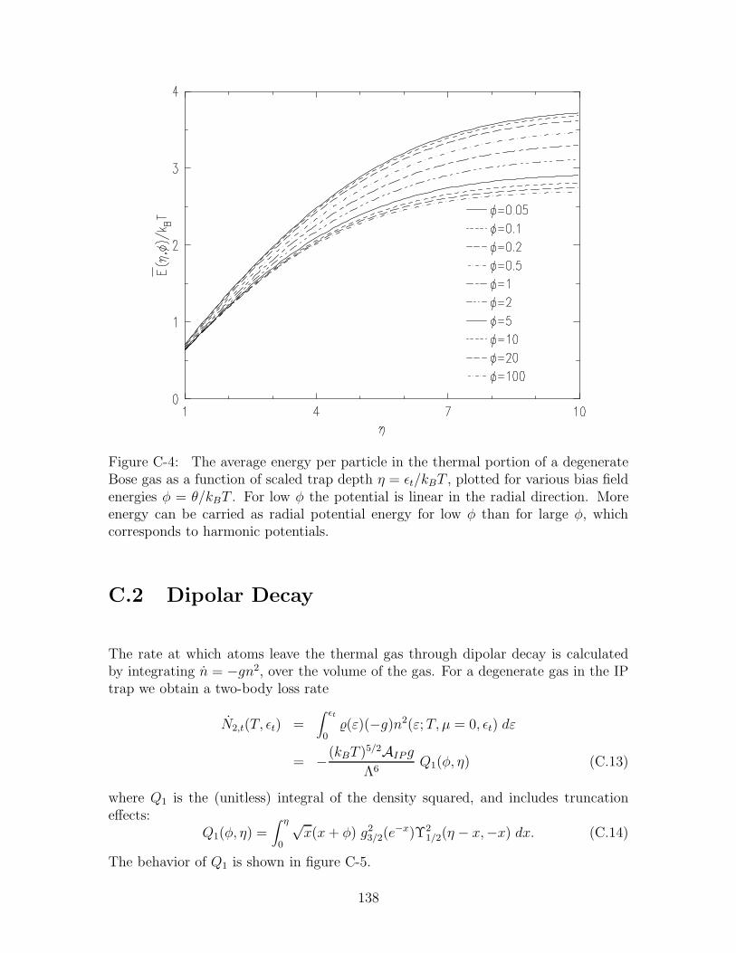
Figure C-4: The average energy per particle in the thermal portion of a degenerateBose gas as a function of scaled trap depth η = ǫt/kBT , plotted for various bias fieldenergies φ = θ/kBT . For low φ the potential is linear in the radial direction. Moreenergy can be carried as radial potential energy for low φ than for large φ, whichcorresponds to harmonic potentials.

C.2 Dipolar Decay

The rate at which atoms leave the thermal gas through dipolar decay is calculatedby integrating n = −gn2, over the volume of the gas. For a degenerate gas in the IPtrap we obtain a two-body loss rate

N2,t(T, ǫt) =∫ ǫt

0(ε)(−g)n2(ε;T, µ = 0, ǫt) dε

= −(kBT )5/2AIPg

Λ6Q1(φ, η) (C.13)

where Q1 is the (unitless) integral of the density squared, and includes truncationeffects:

Q1(φ, η) =∫ η

0

√x(x+ φ) g2

3/2(e−x)Υ2

1/2(η − x,−x) dx. (C.14)

The behavior of Q1 is shown in figure C-5.

138

Figure C-5: Behavior of the squared density integral Q1 as a function of scaled trapdepth η = ǫt/kBT , plotted for various bias field energies φ = θ/kBT . In the figure Q1

is scaled by 0.337 + 0.589φ, the high η asymptote.

The rate at which energy leaves the thermal gas through dipolar decay is

E2,t(T, ǫt) =∫ ǫt

0(ε)(−g)n2(ε;T, µ = 0, ǫt) (ε+ γ(ε)) dε

= −(kBT )7/2AIPg

Λ6Q2(φ, η) (C.15)

where

Q2(φ, η) =∫ η

0

√x(x+ φ) g2

3/2(e−x)Υ2

1/2(η − x,−x)

×(

x+3

2

g5/2(e−x)

g3/2(e−x)

Υ3/2(η − x,−x)Υ1/2(η − x,−x)

)

dx (C.16)

The behavior of Q2 is shown in figure C-6. The average energy carried away by eachparticle that is lost through dipolar relaxation is then C2kBT = kBTQ2/Q1, and isshown in figure C-7. As expected, the average energy lost per particle through dipolarrelaxation is less than E, the average energy per particle throughout the sample(compare figure C-7 with figure C-4), and thus dipolar relaxation leads to heating.Compared to the Maxwell-Boltzmann distribution, the Bose-Einstein distributionhas more particles at lower energy. We thus expect C2 to be smaller, as is seen by

139

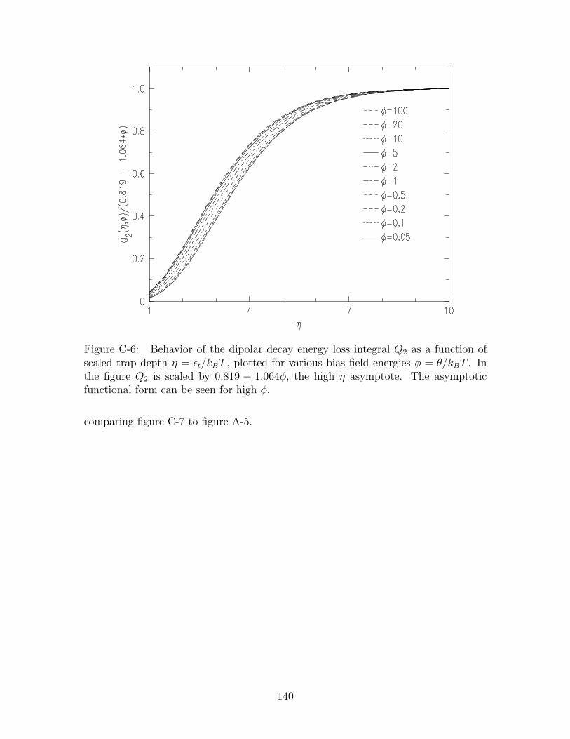
Figure C-6: Behavior of the dipolar decay energy loss integral Q2 as a function ofscaled trap depth η = ǫt/kBT , plotted for various bias field energies φ = θ/kBT . Inthe figure Q2 is scaled by 0.819 + 1.064φ, the high η asymptote. The asymptoticfunctional form can be seen for high φ.

comparing figure C-7 to figure A-5.

140

Figure C-7: Average energy of atoms lost from thermal portion of a degenerate gasthrough dipolar decay, in units of kBT , plotted for µ = 0 and various bias energiesφ = θ/kBT . The asymptotic functional forms for small and large φ are apparent.

141

142

Appendix D

Model of the Dynamics of the

Non-Degenerate Gas

This appendix describes a computer model of the dynamics of the trapped gas, in-cluding evaporation, dipolar decay, and changes of the trap shape and depth. The Csource code is available.

D.1 Overview

We desire a general purpose computer model of the time evolution of our trapped gasto assist in choosing paths through parameter space toward BEC. Previous models[17] employed approximations that are not valid at the low temperatures we wish toaccess and are not easily adaptable to the more complicated trap shapes we wish toemploy.

D.1.1 Approximations

The primary approximation is that the phase space distribution function for thegas is always a Maxwell-Boltzmann truncated at the trap depth. Luiten et al. [26]have confirmed this approximation for slow evaporation. This approximation is validas long as two additional assumptions are valid: (a) instantaneous ergodicity and(b) instantaneous removal of energetic atoms. The validity of these approximationsdepends on some time scales. For approximation (a) we need the time required for thegas to re-equilibrate to be short compared to the speed at which the trap shape anddepth are changed. For approximation (b) we need the energetic atoms to be removedquickly compared to the energy redistribution time. These are the approximationsdescribed in section A.1.1.

D.1.2 Describing the Trap

We make no approximations about the trap shape. Instead the trap is described byenergy and potential energy density-of-states functions (ρ(ǫ) and (ε)) which may

143

involve any number of parameters, all (possibly) time dependent. The energy trun-cation point is also given as a time-dependent parameter.

D.2 Statistical Mechanical Description of the Gas

D.2.1 Variables

We describe the trap by an evaporation energy threshold, ǫt(t), and the density ofstates functions and their set of (time dependent) parameters, ασ(t). These are ourindependent variables. Some function is given by the user to relate these trap shapeparameters to time, the ultimate independent variable.

The primary dependent variables are E and N , the total energy and total pop-ulation of the sample. At each time step during the evolution of the trapped gaswe calculate changes to the total energy, dE, and to the total number of atoms inthe trap, dN . The new value for T may then be calculated from E. If the form ofρ(ǫ) is known, it is often possible to analytically relate T to E. Otherwise T mustbe determined numerically, as is done in this model. The density parameter no istrivially related to N by equation A.13.

D.2.2 Computing Properties of the Gas

The population, N , total energy, E, and density n(r) are computed as described insection A.1.

For notational simplicity, we introduce the functions

ψn ≡∫ ǫt

0dǫ ρ(ǫ) ǫn e−ǫ/kBT (D.1)

andϕn ≡

∫ ǫt

0dǫ ρ(ǫ) ǫn. (D.2)

The Helmholtz free energy is given by A = −kBT logZN , where ZN is the N -particle partition function defined below equation A.8. We can define a “single par-ticle” free energy

A1 ≡ −kBT logZso that A = NA1 + kBT logN !. The entropy is

S = − ∂A

∂T

∣∣∣∣∣V

(D.3)

To keep Veff constant, we replace Z with Veff/Λ3 (using equation A.13) to obtain

S = kB

(

N logZ +3N

2− logN !

)

. (D.4)

144

D.3 Treatment of Physical Effects

The model accounts for cooling due to evaporation, heating due to two-body spinrelaxation, adiabatic trap shape changes, and the skimming of energetic atoms as theenergy threshold is lowered. The finite trap depth is fully integrated into the model.

At each time step we calculate

E = Eevap + E2 + Etrap + Eskim (D.5)

andN = Nevap + N2 + Nskim. (D.6)

Each of these terms is explained below.

D.3.1 Evaporation

Luiten et al. [26] have described the evaporation process, starting from the kineticequation. We summarize their results here. Following section A.2.1, the particle lossrate due to evaporation is

Nevap = −n2o σ v Vevap (D.7)

where σ is the collision cross section, v =√

8kBT/πm is the mean speed,

Vevap = Λ3e−η∫ ǫt

0dǫ ρ(ǫ)

[

(η − 1 − ǫ/kBT )e−ǫ/kBT + e−η]

= Λ3e−η(

(η − 1)ψ0 −ψ1

kBT+ ϕ0e

−η)

(D.8)

is the effective volume for evaporation, and η ≡ ǫt/kBT . The energy loss rate due toevaporation is

Eevap = −n2oσv (ǫt + kBT )Vevap − kBTXevap (D.9)

where

Xevap = Λ3e−η∫ ǫt

0dǫ ρ(ǫ)

[

e−ǫ/kBT − (η + 1 − ǫ/kBT )e−η]

= Λ3e−η(

ψ0 − (η + 1)ϕ0e−η +

ϕ1

kBTe−η

)

(D.10)

D.3.2 Dipolar Spin Relaxation

The particle and energy loss rates N2 and E2 due to dipolar relaxation are given byequations A.20 and A.22 in section A.1.4.

D.3.3 Trap Shape Changes

We assume that the trap shape is changing slowly compared to the transit time of anatom across the trap. Trap shape changes are then adiabatic. We can use dS = 0 to

145

compute dT from changes in the parameters to ρ(ǫ), and eventually obtain dE.

We break dE into its constituents

dE =∂E

∂T

∣∣∣∣∣α

dT +∑

σ

∂E

∂ασ

∣∣∣∣∣T

dασ (D.11)

where the first partial derivative is done at constant trap shape and the sum in thesecond term is over all the trap shape parameters. Since the process is adiabatic,dS = 0. From equation D.4 we see that if dS = 0 and N is fixed we must havedZ = 0. Then we may find dT by writing out dZ. We obtain

dT = −∑

σ∂Z∂ασ

∣∣∣Tdασ

∂Z∂T

∣∣∣ασ

(D.12)

Note that∂ψn∂T

∣∣∣∣∣α

=ψn+1

kBT 2. (D.13)

Remembering that E = Nψ1/ψ0 we get

Etrap =E

ψ1

∑

σ

(

∂ψ1

∂ασ− ψ2

ψ1

∂ψ0

∂ασ

)

ασ. (D.14)

In practice the partial derivatives are evaluated numerically.

D.3.4 Skimming Energetic Atoms

As the trap evaporation threshold is lowered, atoms are skimmed from the top of theenergy distribution. Using equation A.7 we calculate

dNskim =∂N

∂ǫt

∣∣∣∣∣T,ασ

dǫt

Nskim =Nρ(ǫt)e

−η

ψ0ǫt (D.15)

andEskim = ǫt Nskim. (D.16)

D.4 Software Implementation

The evaporation simulator is a set of routines which numerically integrate the differ-ential equations for E and N through time. A user of these routines must write Croutines that describe the trap to the integration routines. The description takes theform of an energy density of states, a potential energy density of states, and an energythreshold above which the energy distribution is truncated. Other code (described

146

below) is also expected to parse the command line and do initialization. Ideally, allof the information that specializes the general evaporation routines to a specific trapand ramp function is contained in a single file in the directory specialized. Thisfile is mentioned in the top level Makefile. Henceforth this file will be referred to asuserfile.

Information about the trap is passed to the evaporation simulation routines in adata structure, mytrap, defined in prog.h. The components of this data structureare pointers to functions and arrays. The data structure is a global variable, and isinitialized by the routine initialize_mytrap in userfile. This routine is called atthe very beginning of the program.

D.4.1 Program Flow

Execution of the program flows as follows. First, initialize_mytrap() is called toset up the data structure. Then a routine, pointed to by mytrap, is invoked to parsethe command line and stash user-provided information into the appropriate arrays.The differential equation integrator is then started. It steps E and N through timeusing the Runge-Kutta routines from Numerical Recipes [111]. At each time step theroutines from userfile are used as follows. First, the threshold and parameters usedfor calculating the density of states are calculated. These might correspond to magnetcurrents or rf field frequencies, as computed for controlling the experiment. Thesevalues are printed to a log file. Since these parameters may often be manipulated intoa form that economizes computation when calculating the density of states, anotherroutine, pointed to by mytrap, is invoked to do this. Finally, we are ready to calculateψn and ϕn for this instant. The new temperature and density are calculated. Theeffects of evaporation, relaxation, skimming, and adiabatic trap shape changes aredetermined, and we are ready for the next step.

D.4.2 Data Structure

The data structure mytrap is referenced often is these calculations, and is the linkbetween user-supplied routines and the general simulation machinery. The entries inthe data structure are:

parse Pointer to a function which parses the command line, obtaining theinitial density and temperature of the simulated gas, and the duration of thesimulation. This information is returned to the simulator. Further informationmight be the beginning and ending currents in certain magnets, shape factorsfor ramps, etc., which would be used to specify the trap shape at each instantof time.

threshold Pointer to a function that gives the energy threshold (atoms withmore than this energy are assumed to escape from the trap), as a function oftime.

147

calc_dos_params Pointer to a function which calculates, at a given time, theparameters used to calculate the density of states. The values calculated herewill be printed in the log file for each time step.

n_dos_params An integer, giving the number of density of states parameterscalculated by calc_dos_params. These are printed in the log file.

precalculate Pointer to a function which manipulates the density of statesparameters to speed up actual calculation of the density of states. For example,in a Ioffe trap the density of states is proportional to the square root of the radialconfinement field. This square root may be calculated here in this routine.

edos A pointer to a routine which returns the energy density of states at agiven energy.

pedos A pointer to a routine which returns the potential energy density of statesat a given energy.

trapspecs An array of information used (possibly) by calc_dos_params andthreshold. These data are not touched by the simulator. The only C file thatlooks at these is userfile.

ntrapspecs Size of the array trapspecs. Only used in file userfile.

Several examples of userfile exist, and may be copied and hacked.

148

Appendix E

Bose-Einstein Velocity Distribution

Function

To find the one-dimensional velocity distribution function which is used in calculatingthe Doppler-sensitive lineshape observed in section 5.3.2 one should use the Bose-Einstein (BE) occupation function instead of the more convenient Maxwell-Boltzmann(MB) occupation function. For a gas at temperature T and chemical potential µ theoccupation function is

f(ǫ;T, µ) =1

e(ǫ−µ)/kBT − 1(E.1)

In this appendix we derive the BE one-dimensional velocity distribution function anduse it to calculate characteristic spectral lineshapes. Truncation effects for a trapof depth ǫt are included, but shown to be small when the laser beam intersects themiddle of the trap and preferentially excites atoms from the deepest part of the trap.In this case, quantum degeneracy is shown to narrow the spectrum.

E.1 Velocity Distribution

The one-dimensional momentum distribution function is obtained in a way analogousto the density, in equation C.2, but the momentum integral is over only two dimen-sions. We define fp(pz) dpz as the probability of an atom having a momentum alongthe z axis within a range dpz of pz; the normalization is 1. The distribution is

fp(pz) =

∫ p⊥,max

0

2πp⊥

e(p2

⊥/2m+p2z/2m+ε−µ)/kBT − 1

dp⊥∫ pmax

0

4πp2

e(p2/2m+ε−µ)/kBT − 1dp

(E.2)

where p⊥ is the momentum perpendicular to z and p2⊥,max/2m = ǫt − ε − p2

z/2mis the maximum allowable kinetic energy perpendicular to z. The denominator ish3n(ε;T, µ, ǫt), calculated above. The numerator can be broken into an expressionwhich neglects truncation and a correction factor Υ0 defined in equation C.3. We

149

Figure E-1: Behavior of the truncation correction factor Υ0 as a function of effectivetrap depth η′, plotted for various effective chemical potentials µ′.

obtain

fp(pz;T, µ, ǫt, ε) =−2πmkBT

h3n(ε;T, µ, ǫt)log

(

1 − exp

(

µ− ε− p2z/2m

kBT

))

×Υ0

(

ǫt − ε− p2z/2m

kBT,µ− ε− p2

z/2m

kBT

)

(E.3)

The behavior of Υ0 is shown in figure E-1. For large η′ truncation is unimportantand Υ0 = 1.

The velocity distribution function is fv(vz) = mfp(mvz). Figure E-2 shows thisdistribution function for various potential energies in the trap. At higher potentialsthe effective chemical potential becomes more negative, and the distributions lookmore classical. Only very near the trap minimum is there significant clumping of thevelocities around zero.

Figure E-3 directly compares the quantum velocity distribution (small µ) withthe classical distribution (large µ). As expected, the classical velocity distributionat ε = 0.1kBT and ε = 1kBT are nearly identical, but differ substantially fromtheir quantum counterparts. For ε = 5kBT the classical and quantum distributionsare nearly identical because even the degenerate gas becomes dilute at this highpotential energy. Truncation effects are important, as evidenced by the sharp cutoffof the velocity distribution.

150

Figure E-2: One dimensional velocity distribution function, plotted for regions withvarious potential energies ε (listed in units of kBT ). The sample temperature isT = 50 µK, the chemical potential is µ = −2×10−7kBT , and the trap depth is 6kBT .The inset reveals part of the ε = 0 distribution that is not visible in the main figure.

E.2 Spectral Signature of Velocity Distribution

The Doppler-sensitive spectrum is a direct measure of the one-dimensional velocitydistribution function fv(vz) through the (radian) frequency shift ∆ = k · v, wherek = 2πz/λ is the wavevector of the radiation and λ = 243.2 nm. The spectrum,S(∆), is given by considering the spectrum of the atoms at each potential energy inthe trap:

S(∆) = S0

∫ ǫt

0dε (ε)n(ε)

∫ vmax

−vmax

dvzfv(vz)δ(∆ − kvz) (E.4)

where mv2max/2 ≡ ǫt − ε is the maximum kinetic energy allowable for atoms with

potential energy ε. The inner integral vanishes if |∆/k| > vmax. The upper integrationlimit on the outer integral thus becomes εmax = ǫt −m∆2/2k2. The spectrum is

S(∆) =S0

hΛ2

∫ εmax

0dε(ε) log

(

1 − e(µ−ε−m∆2/2k2)/kBT)

×Υ0

(

ǫt − ε−m∆2/2k2

kBT,µ− ε−m∆2/2k2

kBT

)

(E.5)

151

Figure E-3: Comparison of one dimensional velocity distributions for samples nearto (far from) quantum degeneracy, having chemical potential µ/kBT = −2 × 10−7

(µ/kBT = −20), plotted with heavy (light) lines. The sample temperature is T =50 µK. The trap depth is 6kBT . The velocity distribution for each chemical potentialis plotted for three different potential energies, listed in units of kBT . For the ε = 5case the two lines overlap; also, truncation effects are clear because of the shalloweffective depth.

This calculation has assumed uniform laser illumination of the sample, has ignoredcoherence effects for atoms that pass repeatedly through the laser beam during ex-citation, has assumed all atoms are driven for identical durations, and has neglectedthe cold-collision frequency shift.

The non-uniform laser illumination can be inserted into equation E.5 as a factorR(ε), an average of the square of the laser intensity over the surface of constantpotential energy ε in a trap potential V (r),

R(ε)I20 =

1

(ε)

∫

d3r I2(ρ, z) δ(ε− V (r)) (E.6)

where I(ρ, z) = I0 exp(−2ρ2/ω2(z)) describes the spatial dependence of the intensityof a Gaussian beam [103]; the beam radius a distance z from the focus is ω(z) =

ω0

√

1 + (z/d)2 where ω0 is the waist radius and d = πω20/λ is the divergence length.

We assume the beam focus is at the center of the trap and the beam is orientedparallel to the cylindrical symmetry axis of the trap. For a Ioffe-Pritchard trap

152

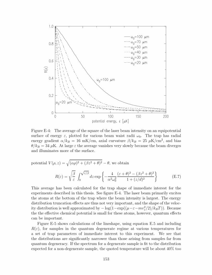
Figure E-4: The average of the square of the laser beam intensity on an equipotentialsurface of energy ε, plotted for various beam waist radii ω0. The trap has radialenergy gradient α/kB = 16 mK/cm, axial curvature β/kB = 25 µK/cm2, and biasθ/kB = 34 µK. At large ε the average vanishes very slowly because the beam divergesand illuminates more of the surface.

potential V (ρ, z) =√

(αρ)2 + (βz2 + θ)2 − θ, we obtain

R(ε) =

√

β

ε

∫√ε/β

0dz exp

− 4

α2ω20

(ε+ θ)2 − (βz2 + θ)2

1 + (z/d)2

(E.7)

This average has been calculated for the trap shape of immediate interest for theexperiments described in this thesis. See figure E-4. The laser beam primarily excitesthe atoms at the bottom of the trap where the beam intensity is largest. The energydistribution truncation effects are thus not very important, and the shape of the veloc-ity distribution is well approximated by − log(1−exp((µ−ε−mv2

z/2)/kBT )). Becausethe the effective chemical potential is small for these atoms, however, quantum effectscan be important.

Figure E-5 shows calculations of the lineshape, using equation E.5 and includingR(ε), for samples in the quantum degenerate regime at various temperatures fora set of trap parameters of immediate interest to this experiment. We see thatthe distributions are significantly narrower than those arising from samples far fromquantum degeneracy. If the spectrum for a degenerate sample is fit to the distributionexpected for a non-degenerate sample, the quoted temperature will be about 40% too

153

Figure E-5: Expected Doppler-sensitive lineshape for a gas near to (far from) thequantum degenerate regime, plotted for samples at various temperatures. The thick(thin) lines are for samples with chemical potential µ/kB = −1×10−4(−5×102) µK,corresponding to the degenerate (non-degenerate) regime. For these calculations ǫt =300 µK, α = 16 mK/cm, β = 25 µK/cm2, θ = 34 µK, and ω0 = 48 µm.

low; the actual temperature is about 1.6 times higher for the conditions of immediateinterest in our experiment.

154

Appendix F

Model of the Dynamics of the

Degenerate Gas

F.1 Overview

This appendix describes a computer model of the dynamics of the degenerate trappedgas, including evaporation and dipolar decay losses from the condensate and thermalgas. As depicted in figure 2-2, the trapped gas is modeled as a system composed oftwo tightly coupled components, the thermal gas and the condensate. We assumethe loss rates from the system are slow compared to the rates of transferring particlesand energy between the two components. A dynamical equilibrium is thus postulated.The results of this model are shown in figure 5-11.

The trap shape is assumed to be static and of the Ioffe-Pritchard form. The depthis fixed. The Bose-Einstein occupation function is used for calculation of dipolar decaylosses from the thermal gas, and the Thomas-Fermi condensate wavefunction is thebasis for calculations of loss from the condensate.

The particle and energy loss rates due to evaporation should be calculated usinga quantum kinetic theory derived from the quantum Boltzmann transport equation.This approach would correctly include the Bose statistics. As a very simple approxi-mation to the desired, but complicated, formulation, we simply apply the evaporationrates calculated for a Maxwell-Boltzmann distribution by Luiten et al. [26] (equationsin section A.2.1). One expects a lower evaporation rate near quantum degeneracy be-cause atom energies are distributed to lower energies relative to the thermal energykBT than is typical in a classical gas. Roughly speaking, the effective η is larger.Another way to think about the situation is to realize that collisions which lead toevaporation occur preferentially among higher energy atoms. As shown in figure 2-1,the Maxwell-Boltzmann distribution calls for many more atoms in these regions ofhigher energy than does the Bose-Einstein distribution in the degenerate regime. Wetherefore reduce the evaporation rate by the adjustable factor F of order 0.4. This Fis the factor mentioned in figure 5-11. Note that the rate of evaporation is reduced,but the energy of the escaping atoms is still approximately (η + 1)kBT .

155

F.2 Simulation Details

The input to the simulation is the initial temperature of the thermal gas and theinitial condensate population (the proper thermodynamic parameters are T and µ; thechemical potential is directly linked to the peak condensate density, which is directlyconnected to the condensate population). The trap shape and depth (α, β, θ, ǫt) areadditional parameters. Finally, a one body loss rate with time constant τ1 is specified.Using this input, the program calculates the total occupation of the trap, NT , andthe total energy, ET , using equations C.6, C.9, and 2.14, and the condensate energyEc = µNc = npU0Nc. It is the total energy and the total population that is evolvedin time. At each time step the temperature is found by numerically solving equationC.9 for the total energy of the thermal gas. We assume µ = 0 for the thermal gasduring the entire simulation. If we allowed µ to vary, then two equations wouldhave to be consistently solved numerically, one for Nt and one for Et (possible, butmore difficult). Once the temperature is found, the occupation of the thermal gasis calculated. The condensate occupation is the total trap occupation minus thethermal occupation, Nc = NT − Nt (we postulate equilibrium between the thermalgas and the condensate, a questionable assumption as discussed in section 2.3.3).The particle and energy loss rates due to dipolar relaxation from the thermal gas andcondensate are calculated using equations C.13 and C.15. Possible one-body lossesare added. The particle and energy loss rates due to evaporation from the thermalgas are calculated for a classical gas of the same peak density as the Bose gas beingsimulated, no = 2.612/Λ3(T ). These rates are multiplied by the correction factor F .The sum of all the particle and energy loss rates for the given time step is returnedto the differential equation stepper routine.

The simulation is stepped through time using the Romberg integration technique[111]. Errors in NT and ET are maintained below the 10−5 level.

F.3 Improvements

One important improvement would be to determine the evaporation rate using thequantum Boltzmann equation, which is based on the correct quantum occupationfunction. This has been done very recently [112].

Further improvements would include treatment of the finite feeding rate of thecondensate from the thermal gas. This bottleneck should be playing a role for thelargest condensates in this thesis, as suggested in section 2.3.3.

156

Appendix G

Trap Shape Uncertainties

In order to calculate various properties of the thermal gas and condensate, it is nec-essary to combine measurements (of density and temperature, for example) withknowledge of the trap shape. In principle the trap shape can be calculated simplyfrom the Biot-Savart law. In practice various complications arise. In this appendixwe discuss these complications and estimate their effect on the trap shape. We con-clude that the trap parameters (radial gradient α and axial curvature β) should haveuncertainties of less than 20%.

The trap shapes used for the experiments in this thesis are created by currentsin 17 superconducting coils. Various compensation schemes are employed to producesteep gradients and large curvatures along the z axis, and shim coils are used to adjustthe bias field. One source of uncertainty is knowledge of the precise geometry of thecoils. Additional uncertainties exist because fields of unknown strength and directionarise from trapped fluxes [17] and magnetized materials in the cryostat.

We first address the stray fields: how can these stray fields influence the trapshape? Let us consider the influence of stray fields on the three Ioffe-Pritchard trapparameters, α, β, and θ. We label the three space coordinates x, y, z, and assume thetrap exhibits cylindrical symmetry about the z axis. A uniform field perpendicular tothe z axis will shift the location of the trap minimum in the plane, but will not affectα, β, or θ. A uniform field parallel to the z axis will shift θ, but not affect α or β. Agradient field with strength B = sx (s is the gradient strength) aligned perpendicularto the z axis will add linearly with α, but will not affect β or θ. A field with strengthB = s z aligned parallel to the z axis will move the trap minimum along the axis andshift θ, but will not affect β. A field with strength B = s z aligned perpendicular tothe z axis will tip the trap symmetry axis away from the z axis, but not affect anyparameters directly. Finally, a field parallel to the z axis and with strength B = s xwill bow the trap and directly perturb all three parameters. Defining the unitless

parameter ǫ =√

1 + (µBs/α)2, we find that α → ǫα, β → β/ǫ, and θ → θ/ǫ.

In the traps of immediate interest in this thesis, the samples are short (a few cm)and very narrow (less than 1 mm in diameter). The radial gradient fields are large(∼ 102 G/cm), and sources of stray fields are far (several cm) from the sample. Thus,we expect only very weak perturbations to the gradient parameter α and the curvatureβ. The parameter θ is easily perturbed, but we can measure it directly, as described in

157

section 4.2.4. Trapped fluxes are expected to exist on the 1 G level, but the distancefrom the sources (superconducting wires) to the trap should cause these fields toappear as simple gradients, which have been shown above to only slightly perturb βand α. Magnetic materials in the cryostat could produce large fields (∼ 10− 100 G),but they are very far away and the field should therefore appear uniform across thetrap (i.e. not appear as gradients). We conclude that stray fields should not perturbthe trap parameters α and β significantly. The parameter θ may be perturbed, butit can be measured directly.

Measurements of θ can be complicated by the effects of gravity: for very coldsamples gravity can pull the atom cloud away from the region of lowest magnetic field,thus making the measurement of θ ambiguous. This distortion becomes importantwhen the gravitational potential energy varies over the height, h, of the cloud bymany times the thermal energy: h ≫ kBT/mg = (0.84 mm/µK)T . For the presentsamples we are far from this limit.

Since stray fields do not strongly effect α or β, the primary uncertainty in knowl-edge of the trap shape arises from uncertainty of the coil winding geometry. The fieldcancelation scheme used to create tight curvature β along the z axis amplifies theuncertainties since the net field is the small difference between multiple large fields.Reasonable uncertainties in the winding geometry (elongations and translations ofcoils on the scale of 5 mm) give rise to no more than 10% changes to the calculatedβ.

A calculation of one of the trap shapes used in chapter 5 is shown in figure G-1,along with analytic fits to the bottom of the potential. The harmonic approximationof the axial curvature of the trap should be precise to the 10% level.

We conclude that uncertainties in the trap shape due to both stray fields andimprecise winding geometry should be below the 20% level.

158

Figure G-1: Calculation of potential energy contours in trap A, along the trap axis(ρ = 0) and offset from the axis by distance ρ = 0.854 mm. A harmonic potentialwith curvature β = 25 ± 3 µK/cm2 is shown. This curvature is used in chapter 5.

159

160

Appendix H

Symbols

Here is a compilation of the symbols used in this thesis, and the pages on which theyare introduced.

symbol descriptionα radial energy gradient in Ioffe-Pritchard trap, p115β axial energy curvature in Ioffe-Pritchard trap, p115Γcol elastic collision rate, p121γ phase space compression efficiency parameter, p126ǫ total energy of a trapped atom, p114ǫt trap depth (energy), p114ε potential energy, p114η scaled trap depth, ǫt/kBT , p116θ bias field energy in Ioffe-Pritchard trap, p115Λ thermal de Broglie wavelength, h/

√2πmkBT , p114

µ chemical potential of sample, p24µB Bohr magneton, eh/2me = 9.274 × 10−24 J/T , p41ρ radial coordinate relative to the trap center, p115ρ(ǫ) total energy density of states, p114(ε) potential energy density of states (differential volume with potential energy ε), p114σ collision cross section for identical particles, 8πa2, p121φ scaled bias field, θ/kBT , p116ωρ radial trap oscillation frequency, p22ωz axial trap oscillation frequency, p22AIP total energy density of states prefactor for IP trap, p114AIP potential energy density of states prefactor for IP trap, p114a scattering length for collisions between two 1S H atoms, 0.648 A, p121B(φ) indicates whether trap is predominantly linear or harmonic in radial direction, p137C(φ, η, f) dependence of heating ratio Hc/Ht on trap shape, p32C2 average energy of atoms lost from thermal gas through dipolar decay, p120, p139D phase space density when far from quantum degeneracy, n0Λ

3, p126E total energy of sample, p117Ec total energy of condensate, p28

161

Et total energy of thermal gas, p136

E2,c energy loss rate due to dipolar decay from the condensate, p28

E2,t energy loss rate due to dipolar decay from the thermal gas, p139F condensate fraction, Nc/(Nt +Nc) = f/(1 + f) , p29f condensate occupation ratio, Nc/Nt , p29Gσλ→φψ dipolar decay event rate for a given channel, p119g dipolar decay rate for a cold gas of d-state atoms, 1.2 × 10−15 cm3/s, p119gk(z) Bose function,

∑∞l=0 z

l/ln, p26Hσ rate at which process σ heats the gas, p32kB Boltzmann’s constant, 1.3807 × 10−29 J/µKm mass of H atom, 1.0078 amuN population, number of atoms, p116Nc population of condensate, p28Nt population of thermal cloud, p135

N2,t particle loss rate due to (two-body) dipolar decay from thermal gas, p138n sample density (atoms per unit volume), p118, p134n0 reference density of thermal gas, p114nc critical density for BEC, 2.612/Λ3(T ), p26ncond condensate density, p27np peak condensate density, p27Q1 unitless dipolar particle decay rate integral, p138Q2 unitless dipolar energy decay rate integral, p139T sample temperature, p114, p24U0 mean field energy per unit density, 4πh2a/m, p27V (r) trap potential energy function, p115Vcond volume of the condensate, assuming a Thomas-Fermi wavefunction, p35Veff effective volume of the sample, p117

v mean speed of particles in a classical gas,√

8kBT/πm, p121

z axial coordinate relative to the trap center, p115Z classical single particle partition function, p116

162

Appendix I

Laboratory Units for Energy

The chart on the following page may prove helpful when comparing the various waysenergy is manifest in atom trapping experiments. The relevant constants are:

constant valuekB 1.381 × 10−29 J/µK, Boltzmann constantµB 9.274 × 10−24 J/T, Bohr magnetonh 6.626 × 10−34 J/Hz, Planck constantmg 1.6411 × 10−28 J/cm, gravitational energy for H

163

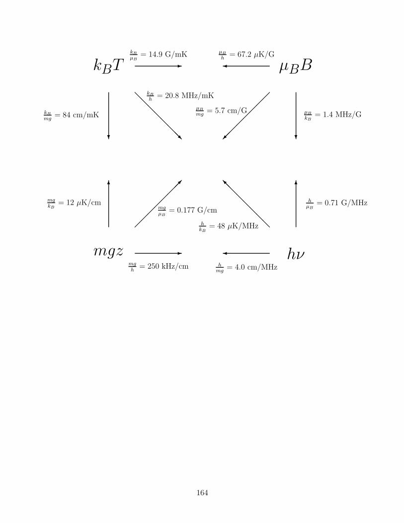
mgz hν

kBT µBB

-

6

mgh

= 250 kHz/cm

mgkB

= 12 µK/cmmgµB

= 0.177 G/cm

?

µB

h= 67.2 µK/G

µB

kB= 1.4 MHz/G

µB

mg= 5.7 cm/G

hmg

= 4.0 cm/MHz

@@

@@

@@

@@I

hkB

= 48 µK/MHz

6

hµB

= 0.71 G/MHz

-

kB

µB= 14.9 G/mK

@@

@@

@@

@@R

kB

h= 20.8 MHz/mK

?

kB

mg= 84 cm/mK

164

Bibliography

[1] W. C. Stwalley and L. H. Nosanow, “Possible “new” quantum systems,” Phys-

ical Review Letters, vol. 36, p. 910, 1976.

[2] M. H. Anderson, J. R. Ensher, M. R. Matthews, C. E. Wieman, and E. A. Cor-nell, “Observation of Bose-Einstein Condensation in a Dilute Atomic Vapor,”Science, vol. 269, p. 198, 1995.

[3] K. B. Davis, M.-O. Mewes, M. R. Andrews, N. J. van Druten, D. S. Durfee,D. M. Kurn, and W. Ketterle, “Bose-Einstein Condensation in a Gas of SodiumAtoms,” Phys. Rev. Lett., vol. 75, p. 3969, 1995.

[4] C. C. Bradley, C. A. Sackett, J. J. Tollet, and R. G. Hulet, “Evidence of Bose-Einstein Condensation in an Atomic Gas with Attractive Interactions,” Phys.

Rev. Lett., vol. 75, p. 1687, 1995.

[5] C. C. Bradley, C. A. Sackett, and R. G. Hulet, “Bose-Einstein condensation oflithium: Observation of limited condensate number,” Physical Review Letters,vol. 78, no. 6, p. 985, 1997.

[6] D. G. Fried, T. C. Killian, L. Willmann, D. Landhuis, S. C. Moss, D. Kleppner,and T. J. Greytak, “Bose-Einstein Condensation of Atomic Hydrogen,” Physical

Review Letters, vol. 81, p. 3811, 1998.

[7] T. C. Killian, D. G. Fried, L. Willmann, D. Landhuis, S. C. Moss, T. J. Greytak,and D. Kleppner, “Cold Collision Frequency Shift of the 1S-2S Transition inHydrogen,” Physical Review Letters, vol. 81, p. 3807, 1998.

[8] M. R. Andrews, C. G. Townsend, H. J. Miesner, D. S. Durfee, D. M. Kurn,and W. Ketterle, “Observation of interference between two Bose condensates,”SCIENCE, vol. 275, pp. 637–641, 1997.

[9] J. Stenger, S. Inouye, D. M. Stamper-Kurn, H.-J. Miesner, A. P. Chikkatur,and W. Ketterle, “Spin domains in ground-state Bose-Einstein condensates,”NATURE, vol. 396, pp. 345–348, 1998.

[10] H.-J. Miesner, D. M. Stamper-Kurn, J. Stenger, S. Inouye, A. P. Chikkatur,and W. Ketterle, “Observation of metastable states in spinor Bose-Einsteincondensates,” submitted to PRL, 1999. cond-mat/9811191.

165

[11] B. P. Anderson and M. A. Kasevich, “Macroscopic quantum interference fromatomic tunnel arrays,” SCIENCE, vol. 282, pp. 1686–1689, 1998.

[12] A. I. Safonov, S. A. Vasilyev, I. S. Yasnikov, I. I. Lukashevich, and S. Jaakkola,“Observation of quasicondensate in two-dimensional atomic hydrogen,” Physi-

cal Review Letters, vol. 81, pp. 4545–4548, 1998.

[13] T. C. Killian, 1S-2S Spectroscopy of Trapped Hydrogen: The Cold Collision

Frequency Shift and Studies of BEC. PhD thesis, Massachusetts Institute ofTechnology, 1999.

[14] C. L. Cesar, Two-Photon Spectroscopy of Trapped Atomic Hydrogen. PhD thesis,Massachusetts Institute of Technology, 1995.

[15] I. A. Yu, Ultracold Surface Collisions: Sticking Probability of Atomic Hydrogen

on Superfluid 4He. PhD thesis, Massachusetts Institute of Technology, 1993.

[16] J. C. Sandberg, Research Toward Laser Spectroscopy of Trapped Atomic Hydro-

gen. PhD thesis, Massachusetts Institute of Technology, 1993.

[17] J. M. Doyle, Energy Distribution Measurements of Magnetically Trapped Spin

Polarized Atomic Hydrogen: Evaporative Cooling and Surface Sticking. PhDthesis, Massachusetts Institute of Technology, 1991.

[18] T. J. Greytak, “Prospects for Bose-Einstein condensation in magneticallytrapped atomic hydrogen,” in Bose-Einstein Condensation (A. Griffin, D. W.Snoke, and S. Stringari, eds.), p. 131, Cambridge University Press, 1995.

[19] recent study, to be published.

[20] M. Morrow, R. Jochemsen, A. J. Berlinsky, and W. N. Hardy, “Zero-field hy-perfine resonance of atomic hydrogen for 0.18 ≤ T ≤ 1 K: the binding energyof H on liquid 4He,” Physical Review Letters, vol. 46, p. 195, 1981. “Errata,”Physical Review Letters, vol. 47, p. 455, 1981. EB = 1.15 K.

[21] R. Jochemsen, M. Morrow, A. Berlinsky, and W. Hardy, “Magnetic resonancestudies of atomic hydrogen at zero field and low temperature: recombinationand binding on liquid helium,” Physica B&C, vol. 110, p. 2108, 1982.

[22] W. N. Hardy, M. D. Hurlimann, and R. W. Cline, “Application of atomichydrogen at low temperatures: The recirculating cryogenic hydrogen maser,”Jpn. J. Appl. Phys., vol. 26, pp. 2065–2072, 1987.

[23] J. M. Doyle, J. C. Sandberg, N. Masuhara, I. A. Yu, D. Kleppner, and T. J.Greytak, “Energy distributions of trapped atomic hydrogen,” Journal of the

Optical Society of America B, vol. 6, p. 2244, 1989.

[24] D. Kleppner, “Trapped atomic hydrogen,” in The Hydrogen Atom (G. F. Bas-sani, M. Inguscio, and T. W. Hansch, eds.), (Berlin), p. 103, Springer-Verlag,1989.

166

[25] C. L. Cesar, D. G. Fried, T. C. Killian, A. D. Polcyn, J. C. Sandberg, I. A. Yu,T. J. Greytak, D. Kleppner, and J. M. Doyle, “Two-Photon Spectroscopy ofTrapped Atomic Hydrogen,” Physical Review Letters, vol. 77, p. 255, 1996.

[26] O. J. Luiten, M. W. Reynolds, and J. T. M. Walraven, “Kinetic theory ofevaporative cooling of a trapped gas,” Physical Review A, vol. 53, p. 381, 1996.

[27] J. T. M. Walraven, “Atomic hydrogen in magnetostatic traps,” in Quantum Dy-

namics of Simple Systems (G.-L. Oppo, S. M. Barnett, E. Riis, and M. Wilkin-son, eds.), (Bristol), p. 315, Institute of Physics Publishing, August 1994.

[28] V. Bagnato, D. E. Pritchard, and D. Kleppner, “Bose-Einstein condensation inan external potential,” Physical Review A, vol. 35, p. 4354, 1987.

[29] J. M. Doyle, J. C. Sandberg, I. A. Yu, C. L. Cesar, D. Kleppner, and T. J. Grey-tak, “Hydrogen in the submillikelvin regime: sticking probability on superfluid4He,” Physical Review Letters, vol. 67, p. 603, 1991.

[30] P. W. H. Pinkse, A. Mosk, M. Weidemuller, M. W. Reynolds, and T. W. Hi-jmans, “One-dimensional evaporative cooling of magnetically trapped atomichydrogen,” Physical Review A, vol. 57, p. 4747, 1998.

[31] D. E. Pritchard, “Cooling neutral atoms in a magnetic trap for precision spec-troscopy,” Physical Review Letters, vol. 51, p. 1336, 1983.

[32] E. L. Surkov, J. T. M. Walraven, and G. V. Shlyapnikov, “Collisionless motionand evaporative cooling of atoms in magnetic traps,” Physical Review A, vol. 53,p. 3403, 1996.

[33] K. Huang, Statistical Mechanics. New York: John Wiley and Sons, 2nd ed.,1987.

[34] W. Pauli Physical Review, vol. 58, p. 716, 1940.

[35] P. Ehrenfest and J. R. Oppenheimer, “Note on the statistics of nuclei,” Physical

Review, vol. 37, no. 4, p. 333, 1931.

[36] F. Dalfovo, S. Giorgini, L. P. Pitaevskii, and S. Stringari, “Theory ofBose-Einstein condensation in trapped gases,” 1998. LANL preprint cond-mat/9806038; accepted for publication in Rev. Mod. Phys.

[37] L. P. Pitaevskii Zh. Eksp. Teor. Fiz., vol. 40, p. 646, 1961. [translation: SovietPhys-JETP 13,451 (1961)].

[38] E. P. Gross Nuovo Cimento, vol. 20, p. 454, 1961.

[39] E. P. Gross, “Hydrodynamics of a superfluid condensate,” Journal of Mathe-

matical Physics, vol. 4, no. 2, p. 195, 1963.

167

[40] M. J. Jamieson, A. Dalgarno, and M. Kimura, “Scattering lengths and effectiveranges for He-He and spin-polarized H-H and D-D scattering,” Physical Review

A, vol. 51, no. 3, p. 2626, 1995.

[41] C. J. Pethick and H. Smith, “Bose-Einstein condensation in dilute gases,”Copenhagen, 1997. http://www.nordita.dk/.

[42] T. J. Greytak and D. Kleppner, “Lectures on spin-polarized hydrogen,” in New

Trends in Atomic Physics (G. Grynberg and R. Stora, eds.), (Amsterdam),p. 1127, Les Houches Summer School, North-Holland, 1982.

[43] D. F. Walls and G. J. Milburn, Quantum Optics. Berlin: Springer-Verlag, 1994.

[44] E. A. Burt, R. W. Ghrist, C. J. Myatt, M. J. Holland, E. A. Cornell, and C. E.Wieman, “Coherence, correlations, and collisions: What one learns about Bose-Einstein condensates from their decay,” Physical Review Letters, vol. 79, no. 3,p. 337, 1997.

[45] T. W. Hijmans, Y. Kagan, G. V. Shlyapnikov, and J. T. M. Walraven, “Bosecondensation and relaxation explosion in magnetically trapped atomic hydro-gen,” Physical Review B, vol. 48, no. 17, p. 12886, 1993.

[46] E. R. I. Abraham, W. I. McAlexander, C. A. Sackett, and R. G. Hulet, “Spec-troscopic determination of the s-wave scattering length of lithium,” Physical

Review Letters, vol. 74, pp. 1315–1318, 1995.

[47] M.-O. Mewes, M. R. Andrews, N. J. van Druten, D. M. Kurn, D. S. Durfee,and W. Ketterle, “Bose-Einstein condensation in a tightly confining dc magnetictrap,” Physical Review Letters, vol. 77, no. 3, p. 416, 1996.

[48] E. Tiesinga, C. J. Williams, P. S. Julienne, K. M. Jones, P. D. Lett, and W. D.Phillips, “A spectroscopic determination of scattering lengths for sodium atomcollisions,” J. Res. Natl. Inst. Stand. Technol., vol. 101, no. 4, pp. 505–520,1996.

[49] J. M. Vogels, C. C. Tsai, R. S. Freeland, S. J. J. M. F. Kokkelmans, B. J.Verhaar, and D. J. Heinzen, “Prediction of Feshbach Resonances in Collisionsof Ultracold Rubidium Atoms,” Phys. Rev. A, vol. 56, p. R1067, 1997.

[50] C. A. Sackett, H. T. C. Stoff, and R. G. Hulet, “Growth and collapse of aBose-Einstein condensate with attractive interactions,” Physical Review Letters,vol. 80, no. 10, p. 2031, 1998.

[51] D. Kleppner, T. J. Greytak, T. C. Killian, D. G. Fried, L. Willmann, D. Land-huis, and S. C. Moss, “Bose-Einstein condensation of atomic hydrogen,” inProceedings of the International School of Physics “Enrico Fermi” Course CXL

(M. Inguscio, S. Stringari, and C. E. Wieman, eds.), (Amsterdam), IOS Press,1999. LANL preprint physics/9812038.

168

[52] D. Jaksch, C. W. Gardiner, K. M. Gheri, and P. Zoller, “Quantum kinetictheory IV. Intensity and amplitude fluctuations of a Bose-Einstein condensateat finite temperature including trap loss,” Physical Review A, vol. 58, no. 2,p. 1450, 1998.

[53] C. Cohen-Tannoudji, B. Diu, and F. Laloe, Quantum Mechanics, vol. 2. Her-mann, 1977.

[54] J. R. Rubbmark, M. M. Kash, M. G. Littman, and D. Kleppner, “Dynamicaleffects at avoided level crossings: A study of the Landau-Zener effect usingRydberg atoms,” Physical Review A, vol. 23, no. 6, p. 3107, 1981.

[55] N. V. Vitanov and K.-A. Suominen, “Time-dependent control of ultracold atomsin magnetic traps,” Physical Review A, vol. 56, no. 6, p. R4377, 1997.

[56] W. Ketterle and N. J. van Druten, “Evaporative cooling of trapped atoms,”in Advances in Atomic, Molecular, and Optical Physics (B. Bederson andH. Walther, eds.), vol. 37, p. 181, Academic Press, 1996.

[57] A. Lagendijk, I. F. Silvera, and B. J. Verhaar, “Spin exchange and dipolarrelaxation rates in atomic hydrogen: Lifetimes in magnetic traps,” Physical

Review B, vol. 33, p. 626, 1986.

[58] P. Lorrain, D. R. Corson, and F. Lorrain, Electromagnetic Fields and Waves.W. H. Freeman and Company, 3rd ed., 1988. p 524-526.

[59] F. Pobell, Matter and Methods at Low Temperatures. Berlin: Springer-Verlag,1992.

[60] Spaulding Composites Co., P. O. Box 867, 1300 S. Seventh St., DeKalb, IL60115-0867, 815-758-0096.

[61] W. R. Abel and J. C. Wheatley, “Experimental thermal conductivity of twodilute solutions of He3 in superfluid He4,” Physical Review Letters, vol. 21,p. 1231, 1968. and references therein.

[62] Folinsbee and Anderson, “The Kapitza resistance to a variety of metallic sur-faces below 0.3 K,” Journal of Low Temperature Physics, vol. 17, p. 409, 1974.

[63] Miller-Stephenson Chemical Co., Inc., Danbury, Connecticut.

[64] Texaco Chemical Company, Houston, Texas.

[65] Emerson & Cumming Inc., Canton, Massachusetts.

[66] Micro Coax Components, Inc., Box 993, Collegeville, PA 19426, 610-489-3700.

[67] M/A-COM, 100 Chelmsford St., PO Box 3295, Lowell, MA 01853, 800-366-2266; model 2058-5214-00.

169

[68] Lakeshore Cryotronics, 64 E. Walnut St., Westerville, OH 43081.

[69] Johnson Matthey Catalog Co., Inc., 30 Bond St., Ward Hill, MA 01835, 800-343-0660; Puratronic 99.999%.

[70] Handy and Harmon, Inc., 5656 S. Pennsylvania Ave., Cudahy, WI 53110, 800-558-3856; alloy Easy-Flow 35.

[71] P. A. Busch, S. P. Cheston, and D. S. Greywell, “Properties of sintered-silverheat exchangers,” Cryogenics, vol. 24, p. 445, 1984.

[72] V. Keith and M. G. Ward, “A recipe for sintering submicron silver powder,”Cryogenics, vol. 24, p. 249, 1984.

[73] Transene Co, Inc, Rowley, MA 01969.

[74] Vacuum Metallurgical Co., Ltd., Japan; North American distributor UlvacNorth America Corp., Kennebunk, Maine.

[75] Epoxy Technology, 14 Fortune Dr., Billerica, MA 01821; 508-667-3805; modelE4110 parts A & B.

[76] Acheson Colloids Company, Port Huron, Michigan.

[77] Miniflex Corporation, 2472 Eastman Ave Unit 29, Ventura, CA 93003-5774;model BC-250-40-14.

[78] CAJON Co., distributed by Cambridge Valve and Fitting, Billerica, MA. 617-272-8270.

[79] model AD811; Analog Devices, One Technology Way, Norwood, MA 02062;617-329-4700.

[80] Dale Co, Inc., 2300 Riverside Blvd., Norfolk, NE 68701-2242; model RCWP-5751 kΩ resistors.

[81] A. G. Martin, K. Helmerson, V. S. Bagnato, G. P. Lafyatis, and D. E. Pritchard,“rf spectroscopy of trapped neutral atoms,” Physical Review Letters, vol. 61,no. 21, p. 2431, 1988.

[82] D. E. Pritchard, K. Helmerson, and A. G. Martin, “Atom traps,” in Atomic

Physics 11 (S. Haroche, J. C. Gay, and G. Grynberg, eds.), (Singapore), p. 179,World Scientific, 1988.

[83] C. L. Cesar and D. Kleppner, “Two-photon Doppler-free spectroscoy of trappedatoms,” Physical Review A, 1999. accepted for publication.

[84] P. Bouyer and M. A. Kasevich, “Heisenberg-limited spectroscopy with degener-ate Bose-Einstein gases,” Physical Review A, vol. 56, pp. R1083–R1086, 1997.

170

[85] J. J. Bollinger, D. J. Wineland, W. M. Itano, and D. J. Heinzen, “Spin squeezingapplied to frequency standards,” in Proceedings of the Fifth Symposium on

Frequency Standards and Metrology (J. C. Bergquist, ed.), (Singapore), pp. 107–114, World Scientific, 1995.

[86] O. J. Luiten, H. G. C. Werij, I. D. Setija, M. W. Reynolds, T. W. Hijmans, andJ. T. M. Walraven, “Lyman-α Spectroscopy of Magnetically Trapped AtomicHydrogen,” Phys. Rev. Lett., vol. 70, p. 544, 1993.

[87] I. D. Setija, H. G. C. Werij, O. J. Luiten, M. W. Reynolds, T. W. Hijmans, andJ. T. M. Walraven, “Optical cooling of atomic hydrogen in a magnetic trap,”Physical Review Letters, vol. 70, p. 2257, 1993.

[88] O. J. Luiten, H. G. C. Werij, M. W. Reynolds, I. D. Setija, T. W. Hijmans,and J. T. M. Walraven, “VUV spectroscopy of magnetically trapped atomic-hydrogen,” Applied Physics B-Lasers and Optics, vol. 59, p. 311, 1994.

[89] P. W. H. Pinkse, A. Mosk, M. Weidemuller, M. W. Reynolds, T. W. Hijmans,and J. T. M. Walraven, “Resonance enhanced two-photon spectroscopy of mag-netically trapped atomic hydrogen,” Physical Review Letters, vol. 79, p. 2423,1997.

[90] T. Udem, A. Huber, B. Gross, J. Reichert, M. Prevedelli, M. Weitz, and T. W.Hansch, “Phase-coherent measurement of the hydrogen 1S-2S transition fre-quency with an optical frequency interval divider chain,” Physical Review Let-

ters, vol. 79, p. 2646, 1997.

[91] M. J. Jamieson, A. Dalgarno, and J. M. Doyle, “Scattering Lengths for Col-lisions of Ground State and Metastable State Hydrogen Atoms,” Mol. Phys.,vol. 87, p. 817, 1996.

[92] L. Willmann. personal communication.

[93] R. Cote and V. Kharchenko, “Quasicondensate droplet formation in a gas oftrapped atomic hydrogen,” 1998. submitted to Physical Review Letters.

[94] J. Stenger, S. Inouye, A. P. Chikkatur, D. M. Stamper-Kurn, D. E. Pritchard,and W. Ketterle, “Bragg spectroscopy of a Bose-Einstein condensate,” Physical

Review Letters, 1999. to be published.

[95] D. M. Stamper-Kurn, M. R. Andrews, A. P. Chikkatur, S. Inouye, H.-J. Miesner,J. Stenger, and W. Ketterle, “Optical confinement of a Bose-Einstein conden-sate,” Physical Review Letters, vol. 80, pp. 2027–2030, 1998.

[96] M. Kozuma, L. Deng, E. W. Hagley, J. Wen, R. Lutwak, K. Helmerson,S. L. Rolston, and W. D. Phillips, “Coherent splitting of Bose-Einstein con-densed atoms with optically induced Bragg diffraction,” Physical Review Let-

ters, vol. 82, pp. 871–875, 1999.

171

[97] J. M. Doyle, B. Friedrich, J. Kim, and D. Patterson, “Buffer-gas loadingof atoms and molecules into a magnetic trap,” Physical Review A, vol. 52,pp. R2515–R2518, 1995.

[98] J. H. Kim, B. Friedrich, D. P. Katz, D. Patterson, J. D. Weinstein, R. DeCar-valho, and J. M. Doyle, “Buffer-gas loading and magnetic trapping of atomiceuropium,” Physical Review Letters, vol. 78, pp. 3665–3668, 1997.

[99] J. D. Weinstein, R. deCarvalho, J. Kim, D. Patterson, B. Friedrich, and J. M.Doyle, “Magnetic trapping of atomic chromium,” Physical Review A, vol. 57,pp. R3173–R3175, 1998.

[100] J. D. Weinstein, R. deCarvalho, T. Guillet, B. Friedrich, and J. M. Doyle, “Mag-netic trapping of calcium monohydride molecules at millikelvin temperatures,”Nature, vol. 395, p. 148, 1998.

[101] H. A. Bethe and E. E. Salpeter, Quantum Mechanics of One- and Two-Electron

Atoms, p. 287. Plenum Publishing Corp., 1977.

[102] M. P. Winters, C. W. Oates, J. L. Hall, and K. P. Dinse, “High-resolutionoptical multiplex spectroscopy,” Journal of the Optical Society of America B,vol. 9, p. 498, 1992.

[103] R. D. Guenther, Modern Optics. New York: John Wiley & Sons, 1990.

[104] H. T. C. Stoof, J. M. V. A. Koelman, and B. J. Verhaar, “Spin-exchange anddipole relaxation rates in atomic hydrogen: Rigorous and simplified calcula-tions,” Physical Review B, vol. 38, p. 4688, 1988.

[105] M.-O. Mewes, M. R. Andrews, D. M. Kurn, D. S. Durfee, C. G. Townsend, andW. Ketterle, “Output coupler for Bose-Einstein condensed atoms,” Physical

Review Letters, vol. 78, pp. 582–585, 1997.

[106] H. F. Hess, “Evaporative cooling of magnetically trapped and compressed spin-polarized hydrogen,” Physical Review B, vol. 34, p. 3476, 1986.

[107] R. van Roijen, J. J. Berkhout, S. Jaakkola, and J. T. M. Walraven, “Exper-iments with atomic hydrogen in a magnetic trapping field,” Physical Review

Letters, vol. 61, p. 931, 1988.

[108] J. J. Sakurai, Modern Quantum Mechanics. Addison-Wesley, 1985.

[109] N. Masuhara, J. M. Doyle, J. C. Sandberg, D. Kleppner, and T. J. Greytak,“Evaporative cooling of spin-polarized atomic hydrogen,” Physical Review Let-

ters, vol. 61, p. 935, 1988.

[110] C. J. Myatt, E. A. Burt, R. W. Ghrist, E. A. Cornell, and C. E. Wieman, “Pro-duction of two overlapping Bose-Einstein condensates by sympathetic cooling,”Physical Review Letters, vol. 78, no. 4, p. 586, 1997.

172

[111] W. H. Press, B. P. Flannery, S. A. Teukolsky, and W. T. Vetterling, Numer-

ical Recipes in C; The Art of Scientific Computing. Cambridge: CambridgeUniversity Press, 1988.

[112] M. Yamashita, M. Koashi, and N. Imoto, “Quantum kinetic theory for evapora-tive cooling of trapped atoms: Growth of Bose-Einstein condensate,” Physical

Review A, vol. 59, pp. 2243–2249, 1999.

173