TURUN YLIOPISTON JULKAISUJAANNALES UNIVERSITATIS TURKUENSIS

SARJA - SER. A I OSA - TOM. 347

ASTRONOMICA-CHEMICA-PHYSICA-MATHEMATICA

STUDIES OF TWO-DIMENSIONAL ATOMIC HYDROGENGAS WITH ELECTRON-SPIN RESONANCE

by

Jarno Järvinen

TURUN YLIOPISTOTurku 2006

From the Wihuri Physical Laboratory

Department of Physics

University of Turku

Turku, Finland

and

National Graduate School in Materials PhysicsHelsinki, Finland

Supervised byDocent Simo Jaakkola and Dr. Sergei Vasiliev, PhD

Wihuri Physical Laboratory

Department of Physics

University of Turku

Turku, Finland

Reviewed byProf. Matti Krusius Prof. Henrik Kunttu

Low Temperature Laboratory Nanoscience Center

Helsinki University of Technology University of Jyväskylä

Finland Finland

OpponentProf. Michael E. Hayden

Department of Physics

Simon Fraser University

Burnaby, B. C.

Canada

ISBN 951-29-2995-3

ISSN 0082-7002

Painosalama Oy - Turku, Finland 2006

Acknowledgements

This work has been carried out in the years 2001-2005 in the Wihuri Physical Laboratory

at the Physics Department of the University of Turku. I want to thank all my friends and

colleagues for creating a friendly working environment during these years.

I want to express my sincere gratitude to my supervisors Dr. Sergei Vasiliev for his

constant support and patient guiding into the world of low temperature experiments, and

to Prof. Simo Jaakkola for helping, guiding, and keeping up good spirit in the group. I

also want to thank Prof. R. Laiho chief of the laboratory and Prof. K. A. Suominen for

illuminating discussions and participating in the seminars of the group. Dr. E. Tjukanoff is

thanked for borrowing experimental devices, and Prof. Kurt Gloos for his outside view and

help during finishing of this thesis. I also want to thank M.Sc. S. Kharitonov and Dr. A.

Safonov from Kurchatov Institute and other visitors who contributed to this work and to the

work of atomic hydrogen group.

A word of thanks also to the technical staff of the University and especially to Mr.

T. Haili for preparing the components needed in the experiments and to Mr. E. Lilja for

providing the liquid helium consumed in the experiments.

And last, I want to thank my beloved Mia for being patient and loving me during these

years.National Graduate School in Materials Physics, Vilho, Yrjö and Kalle Väisälä founda-

tion of Finnish Academy of Science and Letters, Turku University Foundation, and Prof.

Väinö Hovi Stipend Fund are acknowledged for financial support.

Turku, March 2006

Jarno Järvinen

Abstract

In this thesis experiments are described where spin-polarized atomic hydrogen gas was stud-

ied in the 100 mK temperature range with continuous-wave electron-spin resonance (ESR)

at 129 GHz. The chief interest of this work is two-dimensional (2D) H gas adsorbed on

the surface of superfluid 4He. Interatomic interactions and a possibility to observe super-

fluidity in this 2D system were studied. For the experiments a sensitive heterodyne ESR

spectrometer was constructed with its main mm-wave components being installed into a di-

lution refrigerator. ESR signals from both bulk (3D) hydrogen and surface-adsorbed atoms

were detected using a semi-confocal Fabry-Perot resonator. To measure the 2D H densitywe utilized the shift of the surface ESR line with respect to the bulk line position due to

magnetic dipole interactions between the adsorbed H atoms.

The 2D gas was compressed thermally on a small “cold spot” maintained at tempera-

tures ranging from 50 mK to 150 mK. The ESR signal from the surface atoms was found

to be sensitive to the ESR excitation power such that higher powers gave rise to a nonlinear

response of the signal thus causing difficulties in the detection of the surface atoms at low

temperatures. The line shape of the 2D gas spectra was sensitive also to the inhomogeneous

density profile across the cold spot. Origins of the observed linewidth of the surface atoms

are discussed, too.

Simultaneous measurement of the time evolutions of the bulk and surface atomic den-

sities and of the recombination energy enabled us to make the first direct determination of

the surface three-body rate constant Ls3. Being about an order of magnitude smaller than nu-

merous results reported earlier, the value Ls3 = 2(1)× 10−25 cm4s−1 obtained in this work

considerably decreases the discrepancy between the experiments and the theory.

The maximum surface density reached for H in this work was 5.5× 1012 cm−2 corre-

sponding to the 2D phase-space density of 1.6. Information extracted from experiments in

different conditions allowed us to learn of limiting factors to thermal compression. One of

them was an inadequate escape of highly excited molecules from the cold spot which re-

sults in a significant overheating of the surface gas. Possibilities to boost the surface density

further even up to the onset of 2D superfluidity in thermally compressed atomic hydrogen

are considered.

4

Preface

This thesis is based on a series of experiments carried out during the years 2001-2005 and

on seven original papers listed below. The introductory part of the thesis contains also new

unpublished data.

P1. S. Vasilyev, J. Järvinen, A. I. Safonov, A. A. Kharitonov, I. I. Lukashevich,

and S. Jaakkola, Electron-spin-resonance instability in two-dimensional atomic

hydrogen gas, Physical Review Letters 89, 153002 (2002).

P2. S. Vasilyev, J. Järvinen, A. I. Safonov, and S. Jaakkola, Thermal compression of

two-dimensional atomic hydrogen gas, Physical Review A 69, 023610 (2004).

P3. S. Vasilyev, J. Järvinen, A. I. Safonov, and S. Jaakkola, Electron-spin resonance

in quantum degenerate 2D atomic hydrogen gas, Physica B 329-333, 19 (2003).

P4. S. Vasilyev, J. Järvinen, E. Tjukanoff, A. A. Kharitonov, and S. Jaakkola, Cryo-

genic 2 mm wave electron spin resonance spectrometer with application to

atomic hydrogen gas below 100 mK, Review of Scientific Instruments 75, 94

(2004).

P5. T. Peltonen, E. Tjukanoff, J. Järvinen, and S. A. Vasilyev, A Fabry-Perot cav-

ity for millimeter wave ESR detection of hydrogen atoms at low temperatures,

Proceedings of 3rd ESA Workshop on Millimetre Wave Technology and Ap-

plications: Antennas, Circuits and Systems, Eds. J. Mallat, A. Räisänen, J.

Tuovinen, 21-23 May 2003, Espoo, Finland, ESA WPP-212, 2003, p. 447.

P6. J. Järvinen, J. Ahokas, S. Jaakkola, and S. Vasilyev, Three-body recombina-

tion in two-dimensional atomic hydrogen gas, Physical Review A, 72, 052713

(2005).

P7. Jarno Järvinen and Sergei Vasilyev, Atomic hydrogen gas at the surface of su-

perfluid helium, Journal of Physics: Conference Series 19, 186 (2005)

5

My contribution to the papers is described in the following list:

P1. I took part in the measurements and data analysis.

P2. I took part in the measurements, data analysis and writing the paper.

P3. I made the measurements.

P4. I participated in the design, assembly, testing and tuning of the spectrometer

and also wrote part of the paper.

P5. I made the numerical FEM calculations of the resonator model.

P6. I ran the measurements, analyzed the results and wrote most of the paper.

P7. I wrote the paper.

6

Contents

Acknowledgements 3

Abstract 4

Preface 5

1 Introduction 81.1 Background . . . . . . . . . . . . . . . . . . . . . . . . . . . . . . . . . . 8

1.2 Properties of H gas in 2D and 3D . . . . . . . . . . . . . . . . . . . . . . . 10

1.2.1 Atomic states and interatomic potentials . . . . . . . . . . . . . . . 10

1.2.2 Atomic hydrogen adsorbed on liquid helium . . . . . . . . . . . . . 12

1.2.3 Recombination and relaxation . . . . . . . . . . . . . . . . . . . . 15

1.2.4 Electron-spin resonance on H gas . . . . . . . . . . . . . . . . . . 18

2 Experiments on 2D H ↓ 212.1 Experimental apparatus . . . . . . . . . . . . . . . . . . . . . . . . . . . . 21

2.1.1 Cryogenic setup . . . . . . . . . . . . . . . . . . . . . . . . . . . 21

2.1.2 Sample cells and ESR spectrometer . . . . . . . . . . . . . . . . . 24

2.2 Measurement procedures . . . . . . . . . . . . . . . . . . . . . . . . . . . 28

2.2.1 Production and decay of atomic hydrogen . . . . . . . . . . . . . . 28

2.2.2 ESR spectrum of bulk and surface hydrogen gas . . . . . . . . . . 31

3 Results 333.1 ESR line shape of adsorbed hydrogen . . . . . . . . . . . . . . . . . . . . 33

3.1.1 ESR instability . . . . . . . . . . . . . . . . . . . . . . . . . . . . 33

3.1.2 Line broadening due to magnetic field inhomogeneities . . . . . . . 36

3.1.3 Intrinsic broadening due to interatomic collisions . . . . . . . . . . 393.2 Determination of surface gas temperature . . . . . . . . . . . . . . . . . . 41

3.3 Measurement of surface three-body recombination rate . . . . . . . . . . . 42

3.4 Limits of thermal compression . . . . . . . . . . . . . . . . . . . . . . . . 44

4 Conclusions 46

References 47

7

1 Introduction

1.1 Background

Our world is spatially three-dimensional (3D). In some cases the motion of particles is

however tightly restricted to two or even one dimension. A gas adsorbed on the walls of

a container presents an example of a two-dimensional (2D) system. One may ask whether

and how widely the low-dimensional systems differ from the 3D ones in their physical

behaviour? The somewhat surprising answer is that usually physics in 2D is less straight-

forward than in 3D. Quite a general example is the wave equation in 2D space where the

Huygens principle does not hold and the propagation of the wave is different from that in

3D. An incident creating a sharp wave front in 2D space is followed by a slowly decaying

tail [1] which can be seen for example in waves travelling on the surface of water. Good

examples of the effect of dimensionality are also the integer and fractional quantum Hall ef-

fects originating from the discrete quantization of the Landau levels of conduction electrons

in solids having 2D geometry.

Especially after the first observations in 1995 of Bose-Einstein condensation (BEC) in

clouds of trapped alkali atoms [2, 3] there has been interest to observe this phenomenon

also in 2D quantum gases. BEC is a quantum statistical transition in phase space where

the population of the ground state of a boson system becomes macroscopic below a critical

temperature Tc. (A boson is composed of an even number of fermions thus having an inte-ger spin and obeying Bose statistic). From the quantum field theory point of view BEC is a

manifestation of spontaneous breaking of a continuous phase symmetry at Tc. However, in

2D space this is not possible for a uniform system at a finite temperature, as proved by the

Mermin-Wagner-Hohenberg theorem [4, 5, 6]. Superfluidity is in turn regarded as a mani-

festation of BEC, but in 2D the onset of superfluidity is a topological phase transition, the

so-called Berezinskii-Kosterlitz-Thouless (BKT) transition [7, 8], which is different from

BEC [9]. The BKT transition has been observed in thin films of liquid 4He [10] which are

strongly interacting boson systems. The BKT theory predicts the formation of superfluidity

at σΛ2 = 4 due to the binding of vortices into pairs at Tc [8], but it has never been observed

in any weakly interacting system. Here σ is the 2D density of atoms and Λ the thermal de

Broglie wavelength. Above Tc the vortex pairs are free to move and prevent the superfluid

flow.

The theory of Popov [11] introduced the concept of quasi-condensate (QC) where there

are no density fluctuations but phase fluctuates spatially. A QC can be visualized being

divided into domains or "blocks" which are smaller than the phase coherence length but

much larger than the healing length. There is a true condensate inside each block but there

is no phase correlation between the blocks [12]. Popov’s theory is further developed in refs.

8

[13, 14, 15] and Monte Carlo simulations of 2D Bose gas can be found in refs. [16, 17]. A

view emerges that below the BKT transition temperature the 2D superfluid is characterized

by the presence of a QC, but it is unclear what is the relation between the BKT and QC (or

BEC) transitions.

The unique advantage of hydrogen in attaining the conditions of BEC was believed to be

the light atomic mass, which implies a high BEC temperature and prevents the sample from

becoming liquid or solid before quantum effects can take place. This advantage could noteasily overcome two disadvantages of H atoms, their recombination into H2 molecules and

the exceptionally small scattering cross-section. The latter property makes thermalization

of evaporation-cooled atoms in magnetic traps by H-H collisions tedious. Actually after the

first stabilization of spin-polarized atomic hydrogen (H↓) in 1979 [18] it took almost two

decades until the first hydrogen BEC was achieved by a research team at MIT [19] who

used standard cryogenic and evaporative cooling of trapped H↑ down to about 50 µK. At

the same time interest was also directed towards 2D H↓ adsorbed on the surface of liquid

helium and experimental evidence of a quasi-condensate in this system was obtained at

Turku in 1997 [20]. Three-dimensional alkali atom condensates have also been “squeezed”

to dimensional crossover in 1D and 2D traps including optical lattices, [21] magnetic traps

[22] and evanescent wave traps [23]. Phase fluctuations have already been seen in quasi-2D

(and 3D) alkali condensates [24, 25], but the BKT transition has not been observed in them

yet.

In the Turku experiment the formation of a quasi-condensate in H↓ was observed as

a drastic reduction of inelastic three-body collisions when the 2D phase-space density ex-

ceeded σΛ2 ≈ 3 [20]. The sample was compressed at the surface of superfluid 4He film with

the help of a strong magnetic field gradient. Due to distortions of spectra caused by the very

inhomogeneous field it was not possible to combine magnetic compression with magnetic

resonance spectroscopy of surface atoms. Therefore, the method of thermal compression,

first applied to H↓ by T. Mizusaki and coworkers at Kyoto University, [26] was pursued in

the work described in this thesis.

Interactions between H↓ atoms in 2D and with the helium film are other interesting

issues. The exchange interaction is known to be very important in elastic collisions of atoms.

It leads to a shift and broadening of the spectral lines in masers, known as the “clock” or

“cold collision” frequency shift. Recently similar effects were studied in Bose-condensedand normal clouds of alkali vapours with magnetic resonance spectroscopy [27, 28, 29].

But for 2D H↓ gas the clock shift was found [30] to be negligibly small compared to dipolar

shifts, caused by much weaker magnetic interactions. It is not known yet whether this

difference is caused by the reduced dimensionality or by the much larger magnetic field

used.

9

The introductory part of the thesis is organized as follows: Chapter 1 includes, in ad-

dition to this general introduction, short review of interatomic interactions, recombination,

and properties of 2D and 3D atomic hydrogen gas. Details of electron-spin resonance are

also described. Chapter 2 covers the experimental details of the work. Description of differ-

ent parts of the experimental apparatus and of the measurement procedures are considered.

In chapter 3 electron-spin resonance line shapes and temperature of the surface adsorbed

atoms are discussed. Limiting factors preventing to increase 2D H↓ density with thermalcompression are estimated at the end of the chapter. The conclusions of this work are sum-

marized in chapter 4.

1.2 Properties of H gas in 2D and 3D

1.2.1 Atomic states and interatomic potentials

Provided the density of a many-body system formed by the lightest elements is sufficiently

high, quantum effects will create detectable changes in the macroscopic properties of the

system already at relatively high temperatures. Under its own vapour pressure 4He does

not solidify but liquefies at 4.2 K. Except for liquid 3He, which is however composed of

fermions, 4He atoms form the only bulk liquid known to undergo a transition to a superfluid

state at 2.17 K. Unfortunately the relative strong interatomic interactions in liquid helium

effectively mask the quantum effects and complicate the theoretical analysis of the system.

Being even lighter than He, atomic hydrogen is expected to exhibit more pronounced

quantum effects. It turns out in fact that if H atoms interact via the triplet (or symmetric,

denoted as 3Σ+u ) potential [31, 32], the state with parallel electron spins, then the zero-point

energy overwhelms the very weak minimum of the otherwise repulsive triplet potential.

This makes it possible that spin-polarized hydrogen remains gaseous down to the absolute

zero temperature [33]. The attractive singlet (or antisymmetric, denoted as 1Σ+g ) potential

[31, 32] of antiparallel electron spins supports altogether 301 rotational and vibrationalbound states including the stable H2 molecular ground state as much as 52000 K×kB [34,

35] below the continuum. So it is the strong singlet interaction that tends to (re)combine H

atoms into H2 molecules which then solidify already at 14 K.

An external magnetic field B = |B| fixes a preferential orientation for the spins. The

Hamiltonian for a single hydrogen atom in a magnetic field is

H = geµbS ·B+gnµnI ·B+ahS · I, (1)

where ge and gn are electron and nuclear g-factors, respectively, µb and µn are the Bohr and

nuclear magnetons and ah is the hyperfine interaction constant. The Hamiltonian (1) has

four energy eigenstates. These hyperfine states, often labelled from a to d with increasing

10

0 0,1Magnetic field [T]

-0,1

0

0,1E

nerg

y ×

k B [K

]

|a⟩=|↓↑⟩−ε|↑↓⟩

|c⟩=|↑↓⟩+ε|↓↑⟩

|b⟩=|↓↓⟩

|d⟩=|↑↑⟩

ah

ε=a/2geµbBESR

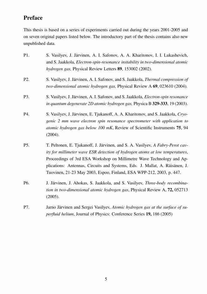
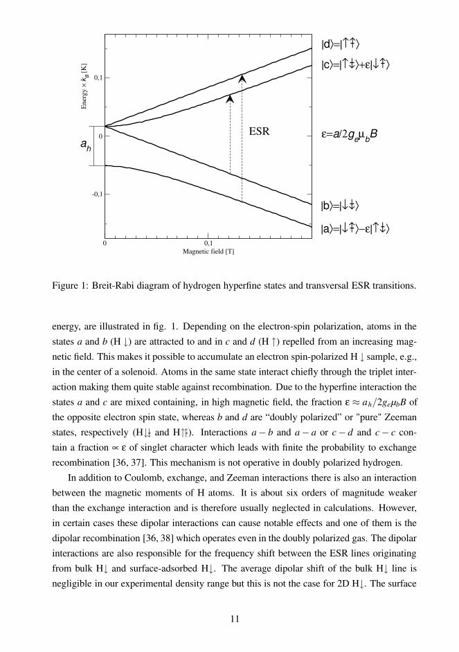
Figure 1: Breit-Rabi diagram of hydrogen hyperfine states and transversal ESR transitions.

energy, are illustrated in fig. 1. Depending on the electron-spin polarization, atoms in the

states a and b (H ↓) are attracted to and in c and d (H ↑) repelled from an increasing mag-

netic field. This makes it possible to accumulate an electron spin-polarized H ↓ sample, e.g.,

in the center of a solenoid. Atoms in the same state interact chiefly through the triplet inter-

action making them quite stable against recombination. Due to the hyperfine interaction the

states a and c are mixed containing, in high magnetic field, the fraction ε ≈ ah/2geµbB of

the opposite electron spin state, whereas b and d are “doubly polarized” or "pure" Zeeman

states, respectively (H�- and H�-). Interactions a− b and a− a or c− d and c− c con-

tain a fraction ∝ ε of singlet character which leads with finite the probability to exchange

recombination [36, 37]. This mechanism is not operative in doubly polarized hydrogen.

In addition to Coulomb, exchange, and Zeeman interactions there is also an interactionbetween the magnetic moments of H atoms. It is about six orders of magnitude weaker

than the exchange interaction and is therefore usually neglected in calculations. However,

in certain cases these dipolar interactions can cause notable effects and one of them is the

dipolar recombination [36, 38] which operates even in the doubly polarized gas. The dipolar

interactions are also responsible for the frequency shift between the ESR lines originating

from bulk H↓ and surface-adsorbed H↓. The average dipolar shift of the bulk H↓ line is

negligible in our experimental density range but this is not the case for 2D H↓. The surface

11

line shift, which is linear in density and depends on the orientation of the magnetic field, is

given by the relation [30]

Bd = −αdP2(cos θ)σ, (2)

where αd is a proportionality constant, θ is the angle between B and the surface normal

and P2 is a Legendre polynomial. The dipolar shift was first observed by Reynolds et al.

[39] and Shinkoda et al. [30], although their experiments suffered from too high ESR

excitation power causing nonlinear effects in the 2D line shape. In this work the value αd =

1.0(1)×10−12 G cm2 [P1, P7] has been measured up to the surface density of σ ≈ 5×1012

cm−2.

1.2.2 Atomic hydrogen adsorbed on liquid helium

The surface of superfluid 4He offers unique properties for creating samples of 2D H↓ gas.

First, the H-He van der Waals interaction is one of the weakest in its class. The effective

interaction potential perpendicular to the He surface was calculated by Guyer and Miller

[40] and Mantz and Edwards [41] who showed that there is only one bound energy eigen-

value Ea for H on the 4He surface. Trapping of H atoms into this bound state will create a

2D gas, in which the average distance of the atoms from the surface and the perpendicular

delocalization length ld are both about 0.6 nm. Secondly, the surface of 4He is completely

uniform. Compared to solids it does not have any periodicity or roughness to disturb the

free particle-like motion of the H atoms along the surface. At temperatures of about 300

mK or less 4He vapour is already in the high-vacuum pressure range.

If one takes into account the elementary surface excitations, called ripplons, the 4He

surface is not completely flat. The amplitude of these quantized capillary waves is only

about 0.1 nm [42, 43] and the wavelength is much longer than the range of the interatomic

interaction [9]. Therefore, ripplons do not influence the H-H scattering. However, in the

cooling of the surface hydrogen the ripplons do play an important role (see below). At

low surface temperatures Tσ the surface density σ of H atoms increases exponentially withdecreasing Tσ. This will increase the number of interatomic collisions and recombination

rate. It is therefore necessary to have the binding of H atoms to the surface as weak as

possible thus extending the sample lifetime and reducing the recombination heating of the

sample. An extreme example of 2D trapping is the magnetic and optical wall-free confine-

ment applied to alkali atoms [22, 23, 44, 45]. However, for H the optical trapping is very

difficult to realize and with the magnetic method it is difficult to reach the 2D confinement

offered by liquid helium surfaces. Anyhow, we may say that the H-He interaction gives a

nice possibility to create a genuine 2D quantum gas of H atoms.

The 2D H gas on a free liquid 4He surface is in dynamical equilibrium with the bulk

12

gas. Continuous exchange of atoms between the bulk and surface-adsorbed phases occurs

at a rate depending exponentially on temperature. A relation between the densities of the

surface and bulk gases, respectively σ and n, in thermal equilibrium is found by equating

the chemical potentials of the two phases. In the high temperature and low density limit this

will lead to the well-known classical equation for the adsorption of a Boltzmann gas:

σ =

(

Tb

Tσ

)32

nΛexp(

Ea

kBTσ

)

, (3)

where Tb is the bulk gas temperature and Tσ is the surface gas temperature. The prefac-

tor (Tb/Tσ)3/2 takes into account the possible temperature difference between the bulk and

surface gases [46]. Alternatively, σ can be expressed by equating the adsorbing and desorb-

ing H atom fluxes. The surface residence time τr is exponentially proportional to the ratio

Ea/kBTσ. Taking quantum correlation effects and the H-H interaction energy into account

τr is given [46] by the relation

1τr

=kBTσs2π~

· 1− exp(−σΛ2)

σΛ2 exp(−Ea +g2U2σ

kBTσ

)

. (4)

Here U2 stands for the H-H mean field interaction energy, g2 is a two-body correlation

function and s ≈ 0.33×Tσ K−1 [47, 48] is the sticking probability of H atoms to the 4He

surface. For non-degenerate identical bosons g2 = 2 and for non-identical or degenerate

bosons g2 = 1. For low densities of σ < 1013 cm−2 and temperatures of about 100 mK

τr ≈ 1.4 ms. The exponential growth of σ, proportional to Ea/kBTσ, is essential for the

thermal compression method used in this work to compress 2D H↓ gas. In an ideal case

a compression factor of about 100 is achieved when the temperature is lowered, e.g., from100 mK to 70 mK.

Eq. (3) also yields Tσ provided Ea, σ and, n are known. The adsorption energy will not

be affected by the solid substrate beneath the liquid 4He layer unless the latter is thinner

than about 20 monolayers [49] (the saturated film is 110 monolayers). There is some scatter

in the experimental values of Ea for H on liquid 4He ranging from 0.9 K to 1.15 K [30,

50, 51, 52, 53]. The values extracted from fits to decay rate equations, including multiple

fitting parameters, are considered to be less accurate than those obtained from magnetic

resonance experiments. The experimental results obtained in the present work support the

value Ea/kB = 1.14(1) K [P1, P2].

Adsorbed hydrogen atoms are in thermal equilibrium with the ripplon system of the

superfluid helium surface. This is because the momentum of an adsorbed atom is relaxed

in a time τp due to emission and scattering of ripplons. At 100 mK the value τp = 3×10−8

s [54] is much shorter than the surface residence time τr, ensuring thermal equilibrium

13

between H and ripplons. The ripplons are in weak thermal contact with the phonon system

of the liquid, from which heat is eventually transferred to the sample cell body. The large

thermal resistance between the ripplons and the phonons of the 4He film creates a bottleneck

in the cooling of the 2D H gas. For the phonon system at a temperature Tph the maximum

cooling power has been calculated to be

Prp = Grp(T20/3

σ −T 20/3ph ), (5)

where Grp = 0.84 Wcm−2K20/3 is the heat conductance of the ripplon-phonon contact [55].

The cooling power is strongly temperature dependent and Grp is smaller than the Kapitza

conductance across, e.g., metal/4He interfaces below 100 mK [56].

The properties of a weakly interacting 2D Bose gas like H↓ are characterized by four

length scales. First there is the 3D s-wave scattering length a3D which defines the 3D

mean-field interaction energy U3 = 4π~2a3D/m between the particles of mass m at low

temperatures. The second length is the effective range of interaction Re, which is generally

not equal to a3D [12, 57]. The third characteristic distance is the de Broglie wavelength

Λ. When Λ � Re the system is in the s-wave scattering limit. The fourth length scale is

the delocalization length ld =√

~2/mEa [12] in the surface-normal direction. In a truly 2D

system ld/a3D . 1 and particle scattering is strongly affected by the confinement making

the interaction always repulsive [58]. Scattering is three-dimensional if ld/a3D & 10 [57].

The intermediate region may be called a quasi-2D region where collisions can be described

by purely 2D scattering but the interaction strength depends on ld [58]. The condition

for weakly interacting gas in the quasi-2D case is |a| � ld [12]. For H on 4He surfacea3D ≈ 0.07 nm [59, and references therein] and ld/a3D ≈ 10. This shows that 2D H is a

weakly interacting system and that short-range interactions are still three-dimensional. This

is also seen in the 2D mean field interaction energy which in the quasi-2D range is given by

[12]

U2 =4π~

2

m1√

2πld/a3D + ln(0.291Ea/Ek)≈ 2

√2π~

2

ma3D

ld(6)

where Ek is the thermal energy of motion in the plane. For 2D H at 100 mK Ea/Ek ≈ 11.4

and the logarithmic term in eq. (6) is only about 5 % which shows that the scattering is

essentially 3D as said above. Eq. (6) gives U2/kB ≈ 3× 10−15 Kcm2 in agreement with

refs. [43, 60]. It is interesting to note that if a3D < 0 the sign of U2 could be changed by

modifying ld [61].

The mean field interaction between atoms in different spin states is known to shift

the radio-frequency resonance lines [28, 27]. This clock or cold collision frequency shift

is caused by the differences of the mean field energy (eq. (6)) between different spin

14

states. The resonance frequency is also shifted differently for condensed and non-condensed

bosons [28]. If the clock shift is larger than the resonance linewidth it can be used as an

indicator of the the quasi-condensation. For 2D H�- the cold collision frequency shift cal-

culated from eq. (6) is about an order of magnitude larger than the dipolar shift [P7] given

by eq. (2). The observed shift is smaller than the calculated one. The clock shift is isotropic

and shifts the line towards higher frequencies, the direction being the same as for the dipolar

shift on the plane perpendicular to the polarizing field. Using this information and the dataof ref. [30] we may conclude that the clock shift is at most 0.4 times the dipolar shift given

by eq. (2).

1.2.3 Recombination and relaxation

The stability of H↓ is determined by the rate of recombination of atoms into H2 molecules

in both bulk and surface phases. Numerous experimental and theoretical studies have been

devoted to the decay kinetics of H↓ [34, 38, 51, 53]. Recombination and the large amount

of energy released in it (4.48 eV per event) tend to prevent the attainment of high enough

densities at low enough temperatures needed for the occurrence of quantum degeneracy. On

the other hand, valuable information on the intrinsic processes of the gas can be obtained

by monitoring the density decay of the H↓ sample and as a matter of fact this has been a

very fruitful method of studying H↓. At densities n . 1016 cm−3 and temperatures ≤ 200

mK bulk recombination is negligible and only surface recombination is significant. This

is because conservation of momentum and energy in all recombination events requires at

least three participating bodies. According to our knowledge no detailed description of H

recombination exists that would take into account the dynamic properties of the He surface.

If one simply assumes that there is no energy exchange between the colliding pair and the

surface, the center of mass momentum along the surface is conserved and recombination

can only take place if the molecule is desorbed at the same time [34].

When the gas is spin-polarized, recombination kinetics is considerably simplified and

only two recombination channels are important. These are surface two-body exchange re-

combination and three-body dipolar recombination. The former occurs only if the collidingH atoms interact through the singlet potential. This implies that only a−a and a−b (see fig.

1) collisions can induce exchange recombination and the rate of this process decreases with

increasing magnetic field as ε2 ∝ B−2. In a pure b-state (H�-) sample there is no exchange

recombination, and the three-body dipolar process is the main source of recombination but

only at high densities. The dipolar interaction is important when the initial three particle

state has no singlet character. When a pair of atoms collide in the dipolar field of a third

atom the variations of the magnetic field induce a singlet component into the interaction of

the pair [36, 38]. This may lead to recombination and, depending on whether the third atom

15

changes or does not change its electron-spin orientation, the event is called single- or double

spin-flip process [34, 62]. In the latter the third atom will recombine in a collision with a

fourth atom. In experiments we measure the total loss rate of atoms and cannot distinguish

between the single and double spin-flip mechanisms in H�-.

In addition to the recombination, decay of H↓ is influenced by the nuclear relaxation

rate between a- and b-states. Two surface relaxation processes can be met in experiments:

impurity induced one-body relaxation and intrinsic two-body relaxation [34]. The formeris a consequence of small spatial fluctuations in the magnetic field caused by magnetic ma-

terials e.g. small grains of iron embedded in the walls during machining. The magnetic

moments of the atoms can also induce eddy currents in a highly conducting surface lead-

ing to the relaxation. Impurity relaxation can be reduced to a negligible level by careful

fabrication of the cell from nonmagnetic materials and by covering the cell walls with a

dielectric layer. Such a layer can be grown from solid H2 by keeping the hydrogen filling

flux on continuously for a long enough time. The two-body surface relaxation process is

anisotropic such that its rate is zero for a surface oriented perpendicular to the polarizing

field [34]. In the sample cells used in the present work there are no walls with high H↓surface density parallel to the polarizing field and the two-body relaxation was found to be

of no importance.

The recombination kinetics is described by rate equations which are coupled first-order

differential equations. The rate constant of one-body relaxation is usually marked as G, the

two-body recombination as K, and the three-body recombination loss rate constant as L3.

For H↓ the equations are

a = −Ge(a−b)−Keabab−2Ke

aaa2

b = Ge(a−b)−Keabab−Le

3b3, (7)

where a and b are the partial bulk densities of the corresponding hyperfine states, and we

have neglected three-body processes which include the a-state. Here, the superscript e

stands for effective bulk rate constants [34] used to transform the intrinsic surface rates

(superscript s) to the effective bulk ones through the adsorption isotherm eq. (3). The

effective rate constants are given by

Ge = AhVh

Λ( TbTσ

)3/2GseEa/kBTσ

Kei j = Ah

VhΛ2( Tb

Tσ)3Ks

i je2Ea/kBTσ

Le3 = Ah

VhΛ3( Tb

Tσ)9/2Ls

3e3Ea/kBTσ ,

(8)

where Ah and Vh are the area and volume of the sample cell. Values of the surface re-

combination rate constants are given in table 1. Due to the large exponential factors surface

16

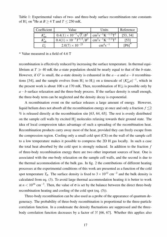
Table 1: Experimental values of two- and three-body surface recombination rate constantsof H↓ on 4He at B ≥ 4 T and T ≤ 250 mK.

Coefficient Value Units Reference

Ksaa 0.4(1)×10−7

√T/B2 cm2s−1K−1/2T2 [53, 34]

Ksab 0.4(1)×10−7T 3/2/B2 cm2s−1K−3/2T2 [53]

Ls3 2.0(7)×10−25 cm4s−1 [P6]*

* Value measured in a field of 4.6 T

recombination is effectively reduced by increasing the surface temperature. In thermal equi-

librium at T � 40 mK the a-state population should be nearly equal to that of the b-state.

However, if Ge is small, the a-state density is exhausted in the a− a and a− b recombina-

tions [34], and the sample evolves from H↓ to H�- on a timescale of (K eaaa)−1, which in

the present work is about 100 s at 170 mK. Then, recombination of H�- is possible only bya−b surface relaxation and the three-body process. If the surface density is small enough,

the three-body term can be neglected and the density decay is exponential.

A recombination event on the surface releases a large amount of energy. However,

liquid helium does not absorb all the recombination energy at once and only a fraction f .2

% is released directly at the recombination site [63, 64, 65]. The rest is evenly distributed

on the sample cell walls by excited H∗2 molecules relaxing towards their ground state. The

idea of local compression takes advantage of such a spreading of the recombination heat.

Recombination products carry away most of the heat, provided they can freely escape from

the compression region. Cooling only a small cold spot (CS) on the wall of the sample cell

to a low temperature makes it possible to compress the 2D H gas locally. In such a case

the total heat absorbed by the cold spot is strongly reduced. In addition to the fraction f

of three-body recombination energy there are two other important sources of heat. One is

associated with the one-body relaxation on the sample cell walls, and the second is due to

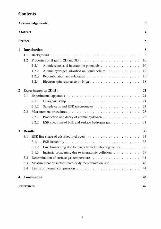
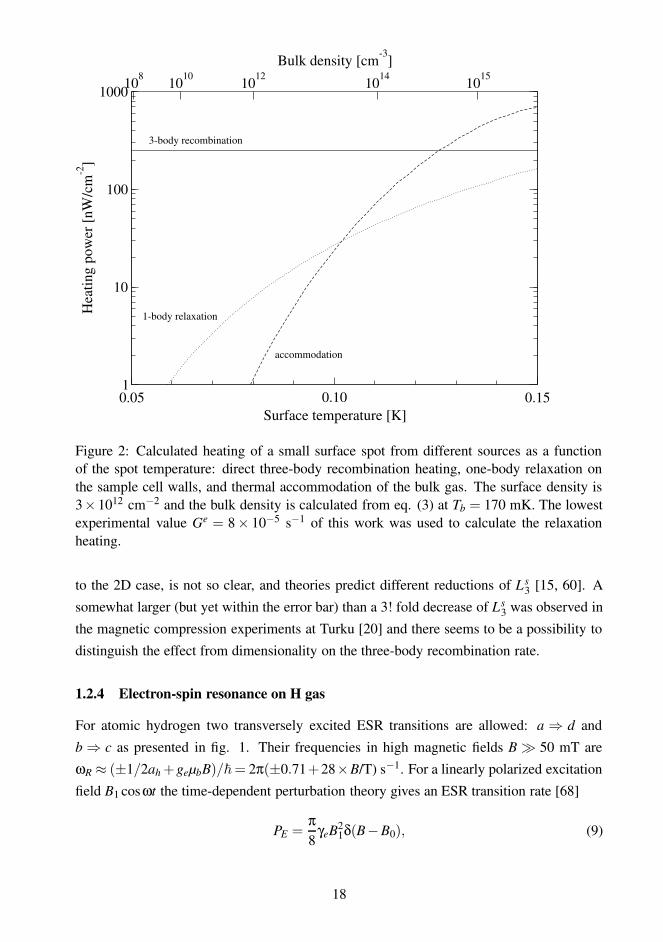
the thermal accommodation of the bulk gas. In fig. 2 the contributions of different heating

processes at the experimental conditions of this work are presented as a function of the cold

spot temperature Tσ. The surface density is fixed to 3× 1012 cm−2 and the bulk density is

calculated from eq. (3). To avoid large thermal accommodation heating it is better to work

at n < 1016 cm−3. Then, the value of σ is set by the balance between the direct three-body

recombination heating and cooling of the cold spot (eq. (5)).

Three-body recombination can be also used as a probe of the appearance of quantum de-

generacy. The probability of three-body recombination is proportional to the three-particle

correlation function. In a condensate the density fluctuations are suppressed and the three-

body correlation function decreases by a factor of 3! [66, 67]. Whether this applies also

17

0.05 0.10 0.15Surface temperature [K]

1

10

100

1000H

eatin

g po

wer

[nW

/cm

-2]

108 1010 1012 1014 1015Bulk density [cm-3]

1-body relaxation

3-body recombination

accommodation

Figure 2: Calculated heating of a small surface spot from different sources as a functionof the spot temperature: direct three-body recombination heating, one-body relaxation onthe sample cell walls, and thermal accommodation of the bulk gas. The surface density is3×1012 cm−2 and the bulk density is calculated from eq. (3) at Tb = 170 mK. The lowestexperimental value Ge = 8× 10−5 s−1 of this work was used to calculate the relaxationheating.

to the 2D case, is not so clear, and theories predict different reductions of Ls3 [15, 60]. A

somewhat larger (but yet within the error bar) than a 3! fold decrease of Ls3 was observed in

the magnetic compression experiments at Turku [20] and there seems to be a possibility to

distinguish the effect from dimensionality on the three-body recombination rate.

1.2.4 Electron-spin resonance on H gas

For atomic hydrogen two transversely excited ESR transitions are allowed: a ⇒ d and

b ⇒ c as presented in fig. 1. Their frequencies in high magnetic fields B � 50 mT are

ωR ≈ (±1/2ah +geµbB)/~ = 2π(±0.71+28×B/T) s−1. For a linearly polarized excitation

field B1 cosωt the time-dependent perturbation theory gives an ESR transition rate [68]

PE =π8

γeB21δ(B−B0), (9)

18

where γe is the electron gyromagnetic ratio and B0 ≈ ωR/γe is the field at resonance. In

practice, due to relaxation processes in the spin system, the delta function in eq. (9) needs

to be replaced by an intrinsic line shape function f i. The intrinsic relaxation processes of

bulk H↓ are very slow, and the observed line shape is determined by inhomogeneities of the

local magnetic field [69, 70, 71]. Yurke et al. [72] found, when considering different line

broadening mechanisms, that the largest contribution to the bulk H↓ line shape is due to

radiation damping [70, 73] yielding a constant line amplitude and a linewidth proportionalto the density. In our experiments this effect is negligibly small for n . 1015 cm−3.

The power absorbed in unit volume from time dependent magnetic field in a lossy para-

magnetic sample is expressed with the help of the complex susceptibility χ(ω) = χ ′(ω)−iχ′′(ω) as [74]

P =ω

2µ0χ′′B2

1, (10)

where µ0 is the vacuum permeability. Comparing equations (9) and (10) it is noticed that

χ′′ ∝ n fi, and the density of paramagnetic particles can be extracted as

n =4

πµ0~γ2e

Z ∞

0χ′′(ω)dω. (11)

In these ESR experiments the signal is detected at a fixed frequency ω0 where the resonator

is tuned. By sweeping ω or B the ESR line is measured. The relation between χ and the

observed ESR signal S in an open Fabry-Perot resonator is derived below. Optical Fabry-

Perot resonators are more conveniently described by the so-called coupled mode approach,

found e.g. in ref. [75], than the equivalent RLC-circuit approach [74] used for closed

resonators. However, following the coupled mode approach eventually gives the same result

as derived for the RLC-circuit.

In the coupled mode approach the so-called mode amplitude u(t) is defined. It is acomplex variable normalized in such a way that uu∗ ≡ |u|2 equals the energy in the resonator.

The resonance frequency of the mode is ω0. The resonator is coupled to an incident wave

si exp(iωt) which is normalized in such a way that |si|2 is the power carried by the incident

wave. The energy in the resonator dissipates causing a decay of the mode amplitude. There

are two different types of power dissipation. The rate of intrinsic dissipation τ−10 is related

to the power absorbed inside the resonator, and the rate of external dissipation τ−1e is due to

a hole coupling the incident wave to the resonator. The quality factor of the loaded resonator

can be expressed with the decay rates as Ql = 12 ω0(τ−1

0 +τ−1e )−1.

The time dependence of u coupled to the incident driving field, provided the power

losses are small, is given by the equation [75]

19

u = iω0u− (1τ0

+1τe

)u+

√

2τe

sieiωt , (12)

In a steady state the solution of eq. (12) is

u =

√

2τe

sieiωt

τ−10 + τ−1

e + i(ω−ω0). (13)

In ESR experiments a reflected wave sr from the cavity is measured. The relation between

si and sr is expressed by the reflection coefficient of the resonator [75]

G0 ≡sr

si=

τ−1e − τ−1

0 − i(ω−ω0)

τ−1e + τ−1

0 + i(ω−ω0). (14)

When a lossy magnetic sample is placed into the resonator it changes the resonance fre-

quency and absorbs an amount ωχ′′(ω)|u|2 of power. This changes the mode decay rate and

the resonance frequency according to

τ−10 + τ−1

e → τ−10 + τ−1

e + 12 ωηχ′′(ω)

ω0 → ω0/√

1+ηχ′(ω).(15)

The filling factor η is defined in the usual way as the ratio between the magnetic field square

integrated over the sample volume and over the whole resonator [74]. When the changes

in eq. (15) are included in eq. (14) the reflection coefficient at the center of the cavity

resonance is given by

G =G0 − iηQlχ(ω)

1+ iηQlχ(ω), (16)

where, assuming small ηχ′, an approximation (1+ηχ′(ω))−1/2 ≈ 1−ηχ′/2 has been used.

The observed ESR signal S is proportional to the changes in the reflected voltage (G −G0)si

from the resonator. The relative change δ of the voltage reflection coefficient is given by

δ ≡ G −G0

G0=

2τ0

τe − τ0· iηQlχ(ω)

1+ iηQlχ(ω). (17)

This result is identical to the result obtained for a closed cavity e.g. in ref. [69]. The real

(imaginary) parts of δ are proportional to the absorption and (dispersion) parts of S. From

eq. (11) it is found for small n that

n ≈ τe − τ0

τ0

2πµ0~γeηQl

Z

Re[δ]dB. (18)

For higher n the relation between χ′′ and Re[δ] is not linear anymore, and n has to be

20

extracted from the dispersion signal [76] or by using the Kramers-Kronig relations [69].

2 Experiments on 2D H ↓

2.1 Experimental apparatus

2.1.1 Cryogenic setup

The experiments were carried out in a top-loading cryostat with two home-made refrigera-

tors, a dilution refrigerator (DR) and a 3He refrigerator. The former cools the sample cell

(SC) and the latter a low-temperature dissociator as illustrated in fig. 3. The dissociator is a

H atom source similar to that used by the Amsterdam group [77]. It is a helical resonator op-

erating at 348 MHz at about 700 mK where the 3He refrigerator has a larger cooling power

than the still of the DR. The base temperature of the DR is 30 mK and its cooling power

at 100 mK is 150 µW. The sample cell (SC) is located in the center of a superconductive

magnet operating at 4.6 T.

The sample cell is thermally linked to the mixing chamber (MC) of the DR, but the link

is weak enough to make it possible to measure the recombination power accurately. Due

to the relatively long distance of about 40 cm from the MC to the SC mechanical thermalanchoring is not convenient for cooling a small cold spot in the cell. Therefore we employed

the dilute 3He−4 He stream of the DR from the mixing chamber as a “coolant” of the cold

spot (CS). At a typical circulation rate of 100 µmoles/s the mixture has a relatively large

specific heat and it flows at the speed of 2 cm/s in a 1.5 mm diameter tube. It allows us

to change the CS temperature in a few seconds by heating the incoming coolant. The ESR

resonator in the SC is connected to the cryogenic mm-wave component block of the ESR

spectrometer [P4] with standard D-band waveguide. A piece of CuNi waveguide is installed

to ensure thermal insulation. The block is thermally anchored to the 1K pot of the DR. A

thermal accommodator of the H flux from the dissociator and the buffer volume for H↓ gas

are cooled by a step heat exchanger of the DR.

Temperatures of the mixing chamber, the sample cell (Tsc), the buffer volume and the

cold spot coolant (Tliq) are measured with RuO2 chip resistors calibrated against the 3He

melting curve thermometer and NBS SRM 768 superconducting fixed-point device. The

calibrations are estimated to be accurate to within 1 mK. Temperatures are monitored and

adjusted with a.c. resistance bridges and temperature controllers (RV-Elektroniikka Oy) and

computer-controlled lock-in amplifiers (Stanford Research Systems).

If the whole dilute stream of the DR would be used to cool the cold spot, the operation of

the DR would be seriously disturbed at high Tliq. Therefore, the stream is divided into two

approximately equal parts as illustrated in fig. 4. One of the streams is taken in a 1.5 mm

21

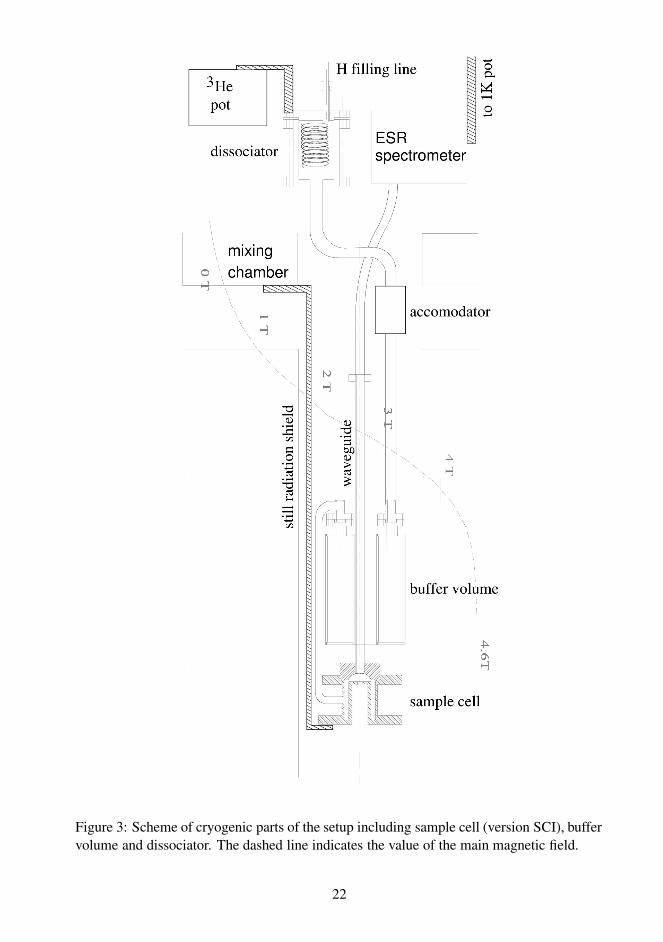
Figure 3: Scheme of cryogenic parts of the setup including sample cell (version SCI), buffervolume and dissociator. The dashed line indicates the value of the main magnetic field.

22

����������������

��������������������

still

still pumping line

heat exhangers

concentratedstream

diluted streammixing chamber

sample cell

cold spot

H volume

sample cell heater

thermal linkcoolant heater

���������������������������������������������������������

���������������������������������������������������������

��������������������������������������������������������������������������������������������������������������������������������������������������������������������

���������������������������������������������������������������������������������

��������������������������������������������������������������������������������������������������������������������������������������������������������������������� bypass loop

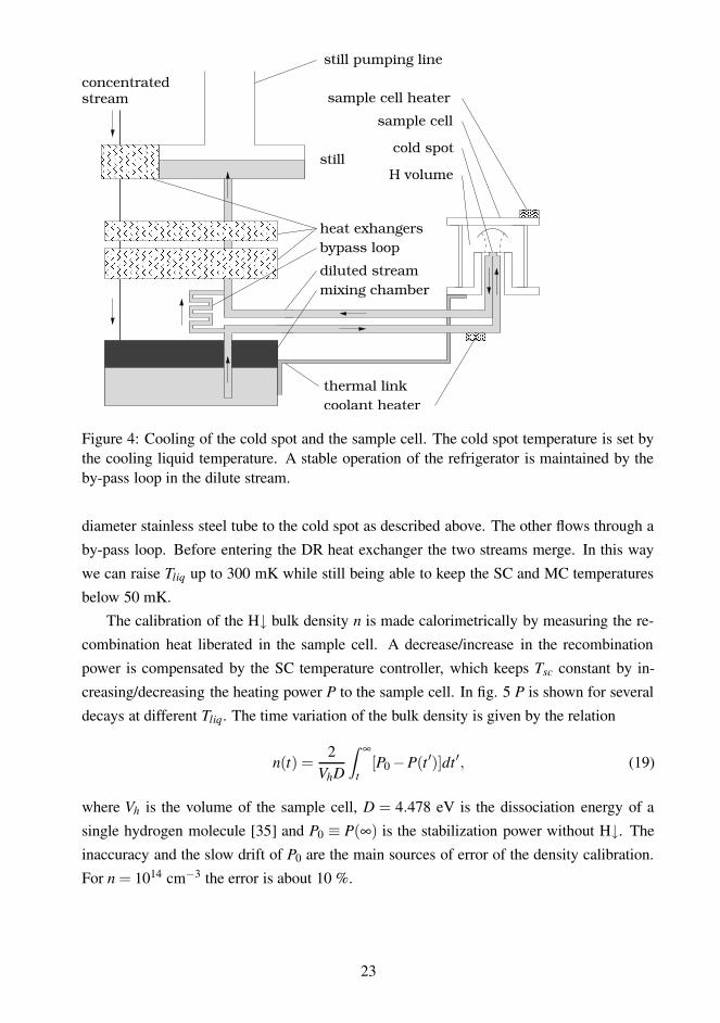
Figure 4: Cooling of the cold spot and the sample cell. The cold spot temperature is set bythe cooling liquid temperature. A stable operation of the refrigerator is maintained by theby-pass loop in the dilute stream.

diameter stainless steel tube to the cold spot as described above. The other flows through a

by-pass loop. Before entering the DR heat exchanger the two streams merge. In this way

we can raise Tliq up to 300 mK while still being able to keep the SC and MC temperatures

below 50 mK.The calibration of the H↓ bulk density n is made calorimetrically by measuring the re-

combination heat liberated in the sample cell. A decrease/increase in the recombination

power is compensated by the SC temperature controller, which keeps Tsc constant by in-

creasing/decreasing the heating power P to the sample cell. In fig. 5 P is shown for several

decays at different Tliq. The time variation of the bulk density is given by the relation

n(t) =2

VhD

Z ∞

t[P0 −P(t ′)]dt ′, (19)

where Vh is the volume of the sample cell, D = 4.478 eV is the dissociation energy of a

single hydrogen molecule [35] and P0 ≡ P(∞) is the stabilization power without H↓. The

inaccuracy and the slow drift of P0 are the main sources of error of the density calibration.

For n = 1014 cm−3 the error is about 10 %.

23

0 2000 4000 6000 8000Time [s]

12

14

16

18

20

22

24

Tem

pera

ture

con

trol

ler f

eedi

ng p

ower

[µW

] TSC=178 mK98 mK

117 mK

129 mK

144 mK

162 mK

2 x time

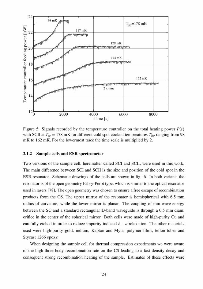
Figure 5: Signals recorded by the temperature controller on the total heating power P(t)with SCII at Tsc = 178 mK for different cold spot coolant temperatures Tliq ranging from 98mK to 162 mK. For the lowermost trace the time scale is multiplied by 2.

2.1.2 Sample cells and ESR spectrometer

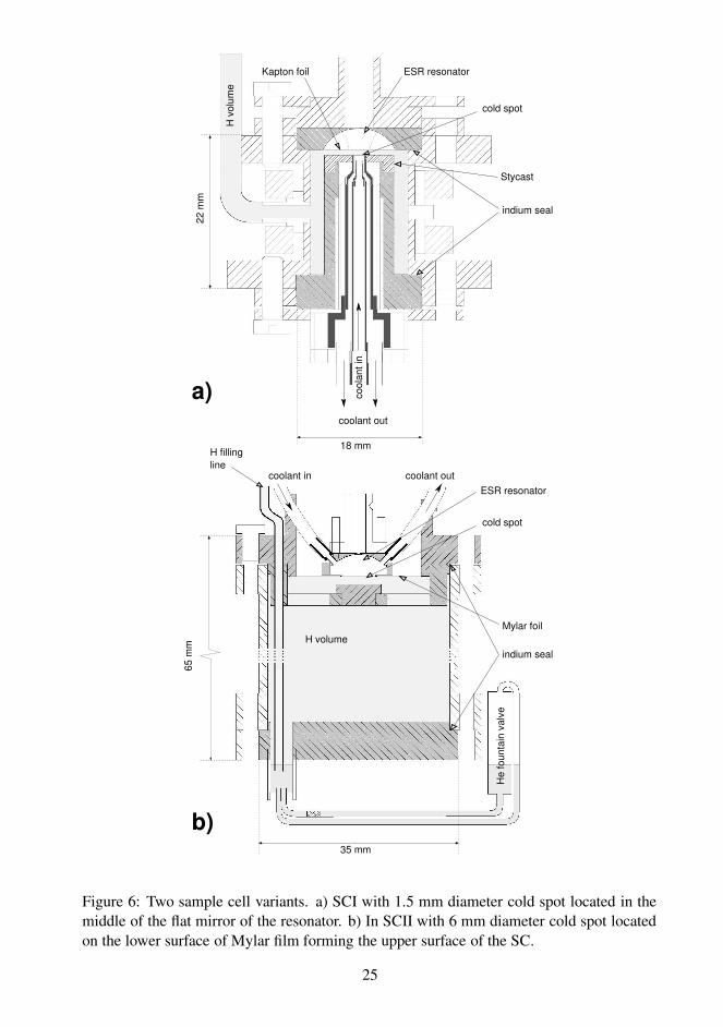
Two versions of the sample cell, hereinafter called SCI and SCII, were used in this work.The main difference between SCI and SCII is the size and position of the cold spot in the

ESR resonator. Schematic drawings of the cells are shown in fig. 6. In both variants the

resonator is of the open geometry Fabry-Perot type, which is similar to the optical resonator

used in lasers [78]. The open geometry was chosen to ensure a free escape of recombination

products from the CS. The upper mirror of the resonator is hemispherical with 6.5 mm

radius of curvature, while the lower mirror is planar. The coupling of mm-wave energy

between the SC and a standard rectangular D-band waveguide is through a 0.5 mm diam.

orifice in the center of the spherical mirror. Both cells were made of high-purity Cu and

carefully etched in order to reduce impurity-induced b− a relaxation. The other materials

used were high-purity gold, indium, Kapton and Mylar polymer films, teflon tubes and

Stycast 1266 epoxy.

When designing the sample cell for thermal compression experiments we were aware

of the high three-body recombination rate on the CS leading to a fast density decay and

consequent strong recombination heating of the sample. Estimates of these effects were

24

a)

b)

lineH filling

coolant out

cool

ant i

n

ESR resonator

indium seal

cold spot

Stycast

Kapton foil

65 m

m22

mm

18 mm

coolant in coolant out

indium seal

ESR resonator

cold spot

Mylar foil

35 mm

He

foun

tain

val

ve

H v

olum

e

H volume

Figure 6: Two sample cell variants. a) SCI with 1.5 mm diameter cold spot located in themiddle of the flat mirror of the resonator. b) In SCII with 6 mm diameter cold spot locatedon the lower surface of Mylar film forming the upper surface of the SC.

25

based on the experimental value Ls3 = 2×10−24 cm4s−1 [51, 52, 79] of the three-body loss

rate constant, as known at the time of the design of SCI. Together with the buffer volume of

38.5 cm3 this fixed the optimal choice of the CS diameter to 1.5 mm, so that the lifetime of

the sample would still be of the order 103 s.

In SCI the cold spot is located in the center of the flat mirror of the resonator where also

the maximum of the ESR excitation field B21 lies. The resonator operates in the TEM002

mode with Ql ≈ 2700. The 3.2 mm diameter of the ESR excitation field is larger than theCS size, which allows the detection of surface atoms outside the CS. The flat mirror of the

ESR resonator is made of a 1 µm thick gold layer evaporated on a 13 µm thick Kapton foil.

The latter is glued on a 0.6 mm thick epoxy disk which has a 1.5 mm diameter hole in

the center. In the hole there are two concentric thin-walled copper tubes in which the 3He-4He mixture stream flows to and from the lower surface of the foil to cool the CS region.

To avoid distortions of the ESR line shape due to too large a number of H atoms [76] the

volume of the bulk gas is restricted by another Kapton foil placed 0.8 mm above the flat

mirror. Hydrogen atoms are fed from the buffer volume to the SC through a 5 cm long

Teflon tube. The buffer volume temperature is kept at about 350 mK, which is ideal for

storing H↓ atoms.

A series of experiments carried out [P1, P2] led to a better understanding of the be-

haviour of 2D H gas and revealed certain disadvantages in the construction of SCI. The

most important result was that the three-body recombination rate on the CS turned out to be

much smaller than expected. Three-body recombination was not dominating the decay and

in fact the contribution of the CS was hardly discernible from the one-body relaxation rate

on the sample cell and buffer volume walls. By "switching" the thermal compression on

and off during the decays we extracted an upper limit estimate Ls3 . 2×10−25 cm4s−1 [P2],

which is 10 times smaller than expected. Also the thermal contact between the spot and the

cell in SCI was too strong, not allowing to work with a large enough temperature difference

between the CS and the SC. Lowering Tsc strongly increased the one-body relaxation rate.

Another drawback was that the ESR line shape of 2D hydrogen on the CS was distorted

by the inhomogeneous density distribution, which depends on the temperature difference

between the spot and the cell.

In the later version of the sample cell, SCII (fig. 6b), the CS radius is increased to 3

mm. The "ceiling" of the H volume is a 20 µm Mylar film. An epoxy ring together with thespherical mirror is glued on the top of the center of the Mylar foil, outside the H volume,

forming a space filled with circulating 3He-4He mixture. This construction improves the

thermal insulation between the CS and the SC. The horizontal extent of the ESR excitation

field on the CS is smaller than the cold spot which makes the ESR signal originate from

the central part of the CS only. This decreases the line broadening due to a possible density

26

inhomogeneity and gives an opportunity to study the intrinsic line shape. Due to good

thermal isolation between the CS and the SC we are able to work at higher cell temperatures.

This made it also possible to remove the buffer volume and to increase the volume of the

cell to 40 cm3. The cell geometry is designed to be simple, making it easier to cover its

inner surfaces with a polymer foil and epoxy. These measures allowed us to reduce the

one-body relaxation rate to a negligible level. To avoid the escape of atoms and excited

molecules from the SC, we installed a 4He fountain valve into the H filling line. The valveis controlled with a heater and the helium level is measured with a capacitive level gauge.

The ESR resonators were designed to detect both 3D gas in the cell volume and 2D

gas adsorbed on the CS. They were constructed relying upon the Gaussian beam wave

theory for laser resonators [78]. When a proper resonance mode was found, the excitation

field profiles B21(r) were calculated numerically by solving the Helmholtz equation with

ideally conducting boundary conditions. The calculation of B21(r) in SCI was compared

with measurements of B21(r) carried out with an oversized test resonator [P5]. B2

1(r) was

used when calculating the effective volume of the resonator from the relation

Ve =1

max[B21]

Z

B21(r)d

3r, (20)

where the integral is taken over the hydrogen volume in the resonator. The effective area Ae

of the CS is calculated similarly by integrating over the area of the flat mirror. The values

of Ve and Ae are important in the calibration of the ESR signals against the bulk and surface

densities.

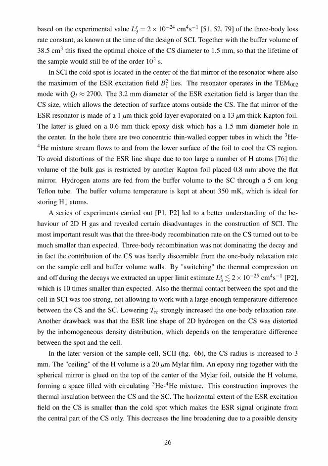
The resonator of SCII is shown in fig. 7 together with the calculated B21(r). The res-

onator operates in the TEM003 mode and its Ql is about half of that of SCI. The field profile

in the resonator is distorted by the dielectric Stycast part and it is not very well described

by the Gaussian beam wave theory. These disturbances can be seen in the two lowest nodes

in fig. 7. Three quarters of the resonator is filled with the coolant liquid whose dielectric

constant 1.05 depends slightly on the 3He/4He concentration ratio which together with the

resonator frequency depends on temperature. Fortunately this dependence is rather weak at

Tliq . 100 mK and does not noticeably disturb the stability of the ESR signal. On the other

hand, by heating the coolant to temperatures of the order of 1K leads to an ESR resonator

frequency shift of about 50 MHz and helps to find the resonance frequency after the cool

down of the spectrometer from room temperature. The ESR spectrometer is a home-built

129 GHz cryogenic heterodyne system. Its technical details are described in ref. [P4]. The

spectrometer is capable of detecting simultaneously both absorption and dispersion signals

with the detection sensitivity of about 109 spins/G for 20 pW mm-wave excitation power.

27

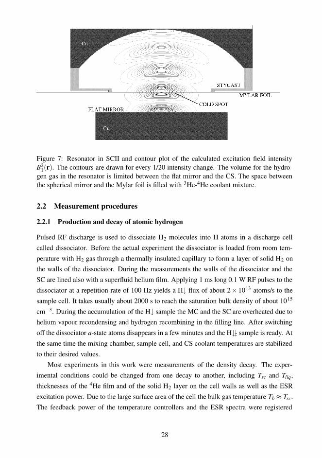
Figure 7: Resonator in SCII and contour plot of the calculated excitation field intensityB2

1(r). The contours are drawn for every 1/20 intensity change. The volume for the hydro-gen gas in the resonator is limited between the flat mirror and the CS. The space betweenthe spherical mirror and the Mylar foil is filled with 3He-4He coolant mixture.

2.2 Measurement procedures

2.2.1 Production and decay of atomic hydrogen

Pulsed RF discharge is used to dissociate H2 molecules into H atoms in a discharge cell

called dissociator. Before the actual experiment the dissociator is loaded from room tem-

perature with H2 gas through a thermally insulated capillary to form a layer of solid H2 onthe walls of the dissociator. During the measurements the walls of the dissociator and the

SC are lined also with a superfluid helium film. Applying 1 ms long 0.1 W RF pulses to the

dissociator at a repetition rate of 100 Hz yields a H↓ flux of about 2× 1013 atoms/s to the

sample cell. It takes usually about 2000 s to reach the saturation bulk density of about 1015

cm−3. During the accumulation of the H↓ sample the MC and the SC are overheated due to

helium vapour recondensing and hydrogen recombining in the filling line. After switching

off the dissociator a-state atoms disappears in a few minutes and the H�- sample is ready. At

the same time the mixing chamber, sample cell, and CS coolant temperatures are stabilized

to their desired values.

Most experiments in this work were measurements of the density decay. The exper-

imental conditions could be changed from one decay to another, including Tsc and Tliq,

thicknesses of the 4He film and of the solid H2 layer on the cell walls as well as the ESR

excitation power. Due to the large surface area of the cell the bulk gas temperature Tb ≈ Tsc.

The feedback power of the temperature controllers and the ESR spectra were registered

28

4 5 6 7 8 9 101/Tb [1/K]

10-5

10-4

Vh/A

hGe x

T1/

2 [K1/

2 cm3 /s

] No coati

ng

72 h

y = 1.6×10-07Exp( 0.78/Tb)

60 h

182 h

Figure 8: VhAh

Ge√Tb plotted versus 1/Tb with different accumulation times for the solid H2layer. The closed circles are the saturated values after accumulating for 300 hours or more.The dashed line is an exponential fit to the saturated values. The open circles show resultsfor shorter accumulation times as indicated. The dotted lines display the temporal sequencein which the open circles were measured.

during the decay. In order to determine the power P0 needed in the density calibration (eq.

(19)) the data collection was continued until the atomic hydrogen signal had become com-

pletely extinct. The spectra were obtained by sweeping the magnetic field across the bulk

and surface b− c resonances.

The ESR excitation power could be varied within four orders of magnitude. The ESR-

induced recombination of the sample was used to estimate the absolute value of the field

B1 (eq.(9)) in the resonator. At the highest excitation levels we observed B1 ≈ 10−2 G.

When the excitation was lowered by an order of magnitude, the destruction of the sample

due to ESR was negligible compared to the natural decay rate. However, another order of

magnitude decrease was required to avoid the instability effects in the 2D ESR signals [P1].

The rate of b−a nuclear relaxation is influenced by the quality of the sample cell walls.

Although much care was taken to reduce the amount of possible magnetic impurities in the

walls, the relaxation rate was always high in the beginning of each series of experiments.Therefore we used the well-known method [80] to build up a layer of solid H2 on the SC

walls by keeping the H↓ flux continuously on even for a week. This decreased the relaxation

29

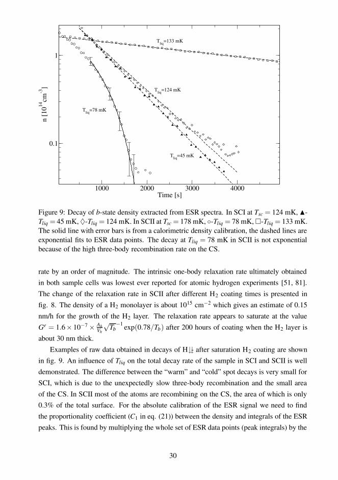
1000 2000 3000 4000Time [s]

0.1

1

n [1

014cm

-3]

Tliq=133 mK

Tliq=78 mK

Tliq=124 mK

Tliq=45 mK

Figure 9: Decay of b-state density extracted from ESR spectra. In SCI at Tsc = 124 mK, N-Tliq = 45 mK, ♦-Tliq = 124 mK. In SCII at Tsc = 178 mK, ◦-Tliq = 78 mK, �-Tliq = 133 mK.The solid line with error bars is from a calorimetric density calibration, the dashed lines areexponential fits to ESR data points. The decay at Tliq = 78 mK in SCII is not exponentialbecause of the high three-body recombination rate on the CS.

rate by an order of magnitude. The intrinsic one-body relaxation rate ultimately obtained

in both sample cells was lowest ever reported for atomic hydrogen experiments [51, 81].

The change of the relaxation rate in SCII after different H2 coating times is presented in

fig. 8. The density of a H2 monolayer is about 1015 cm−2 which gives an estimate of 0.15

nm/h for the growth of the H2 layer. The relaxation rate appears to saturate at the value

Ge = 1.6× 10−7 × AhVh

√Tb

−1 exp(0.78/Tb) after 200 hours of coating when the H2 layer is

about 30 nm thick.

Examples of raw data obtained in decays of H�- after saturation H2 coating are shown

in fig. 9. An influence of Tliq on the total decay rate of the sample in SCI and SCII is well

demonstrated. The difference between the “warm” and “cold” spot decays is very small for

SCI, which is due to the unexpectedly slow three-body recombination and the small area

of the CS. In SCII most of the atoms are recombining on the CS, the area of which is only0.3% of the total surface. For the absolute calibration of the ESR signal we need to find

the proportionality coefficient (C1 in eq. (21)) between the density and integrals of the ESR

peaks. This is found by multiplying the whole set of ESR data points (peak integrals) by the

30

constant C1 and fitting it to the integrated temperature controller signal with C1 being a free

parameter. Decays with the warm spot are very well described by exponential functions.

This implies that the temperature of the cell walls remains constant during the decays and

that the decays are of the first order in density as caused by one-body relaxation.

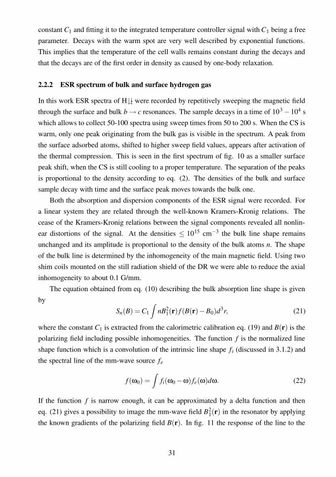
2.2.2 ESR spectrum of bulk and surface hydrogen gas

In this work ESR spectra of H�- were recorded by repetitively sweeping the magnetic field

through the surface and bulk b → c resonances. The sample decays in a time of 103 −104 s

which allows to collect 50-100 spectra using sweep times from 50 to 200 s. When the CS is

warm, only one peak originating from the bulk gas is visible in the spectrum. A peak from

the surface adsorbed atoms, shifted to higher sweep field values, appears after activation of

the thermal compression. This is seen in the first spectrum of fig. 10 as a smaller surface

peak shift, when the CS is still cooling to a proper temperature. The separation of the peaks

is proportional to the density according to eq. (2). The densities of the bulk and surface

sample decay with time and the surface peak moves towards the bulk one.

Both the absorption and dispersion components of the ESR signal were recorded. Fora linear system they are related through the well-known Kramers-Kronig relations. The

cease of the Kramers-Kronig relations between the signal components revealed all nonlin-

ear distortions of the signal. At the densities ≤ 1015 cm−3 the bulk line shape remains

unchanged and its amplitude is proportional to the density of the bulk atoms n. The shape

of the bulk line is determined by the inhomogeneity of the main magnetic field. Using two

shim coils mounted on the still radiation shield of the DR we were able to reduce the axial

inhomogeneity to about 0.1 G/mm.

The equation obtained from eq. (10) describing the bulk absorption line shape is given

by

Sn(B) = C1

Z

nB21(r) f (B(r)−B0)d3r, (21)

where the constant C1 is extracted from the calorimetric calibration eq. (19) and B(r) is thepolarizing field including possible inhomogeneities. The function f is the normalized line

shape function which is a convolution of the intrinsic line shape f i (discussed in 3.1.2) and

the spectral line of the mm-wave source fe

f (ω0) =Z

fi(ω0 −ω) fe(ω)dω. (22)

If the function f is narrow enough, it can be approximated by a delta function and then

eq. (21) gives a possibility to image the mm-wave field B21(r) in the resonator by applying

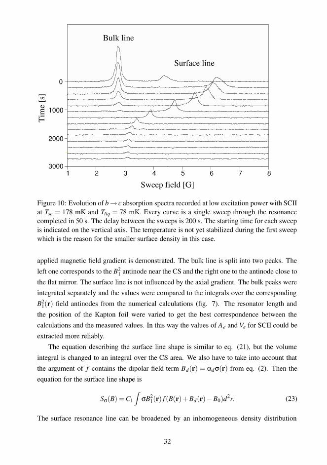
the known gradients of the polarizing field B(r). In fig. 11 the response of the line to the

31

Sweep field [G]

Tim

e [s

]

1 2 3 4 5 6 7 83000

2000

1000

0

Surface line

Bulk line

Figure 10: Evolution of b→ c absorption spectra recorded at low excitation power with SCIIat Tsc = 178 mK and Tliq = 78 mK. Every curve is a single sweep through the resonancecompleted in 50 s. The delay between the sweeps is 200 s. The starting time for each sweepis indicated on the vertical axis. The temperature is not yet stabilized during the first sweepwhich is the reason for the smaller surface density in this case.

applied magnetic field gradient is demonstrated. The bulk line is split into two peaks. The

left one corresponds to the B21 antinode near the CS and the right one to the antinode close to

the flat mirror. The surface line is not influenced by the axial gradient. The bulk peaks wereintegrated separately and the values were compared to the integrals over the corresponding

B21(r) field antinodes from the numerical calculations (fig. 7). The resonator length and

the position of the Kapton foil were varied to get the best correspondence between the

calculations and the measured values. In this way the values of Ae and Ve for SCII could be

extracted more reliably.

The equation describing the surface line shape is similar to eq. (21), but the volume

integral is changed to an integral over the CS area. We also have to take into account that

the argument of f contains the dipolar field term Bd(r) = αdσ(r) from eq. (2). Then the

equation for the surface line shape is

Sσ(B) = C1

Z

σB21(r) f (B(r)+Bd(r)−B0)d2r. (23)

The surface resonance line can be broadened by an inhomogeneous density distribution

32

0 1 2 3 4 5 6 7Sweep field [G]

0

1

2

3

4

ESR

sig

nal [

arb.

]

0.41 G Axial gradient on

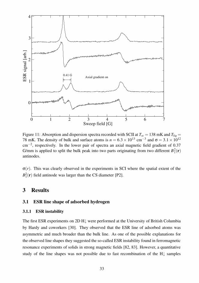
Figure 11: Absorption and dispersion spectra recorded with SCII at Tsc = 138 mK and Tliq =78 mK. The density of bulk and surface atoms is n = 6.3× 1013 cm−3 and σ = 3.1× 1012

cm−2, respectively. In the lower pair of spectra an axial magnetic field gradient of 0.37G/mm is applied to split the bulk peak into two parts originating from two different B2

1(r)antinodes.

σ(r). This was clearly observed in the experiments in SCI where the spatial extent of the

B21(r) field antinode was larger than the CS diameter [P2].

3 Results

3.1 ESR line shape of adsorbed hydrogen

3.1.1 ESR instability

The first ESR experiments on 2D H↓ were performed at the University of British Columbia

by Hardy and coworkers [30]. They observed that the ESR line of adsorbed atoms was

asymmetric and much broader than the bulk line. As one of the possible explanations forthe observed line shapes they suggested the so-called ESR instability found in ferromagnetic

resonance experiments of solids in strong magnetic fields [82, 83]. However, a quantitative

study of the line shapes was not possible due to fast recombination of the H↓ samples

33

1

2

3

ESR

signal [arb.]

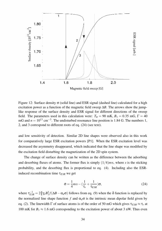
Figure 12: Surface density σ (solid line) and ESR signal (dashed line) calculated for a highexcitation power as a function of the magnetic field sweep ∆B. The arrows show the jump-like response of the surface density and ESR signal for different directions of the sweepfield. The parameters used in this calculation were: Tσ = 90 mK, B1 = 0.35 mG, Γ = 40mG and n = 1013 cm−3. The undisturbed resonance line position is 1.84 G. The numbers 1,2, and 3 correspond to different roots of eq. (24) (see text).

and low sensitivity of detection. Similar 2D line shapes were observed also in this work

for comparatively large ESR excitation powers [P1]. When the ESR excitation level was

decreased the asymmetry disappeared, which indicated that the line shape was modified by

the excitation field disturbing the magnetization of the 2D spin system.

The change of surface density can be written as the difference between the adsorbing

and desorbing fluxes of atoms. The former flux is simply (1/4)nvs, where s is the sticking

probability, and the desorbing flux is proportional to eq. (4). Including also the ESR-

induced recombination time τESR we get

σ =14

nvs− (1τr

+1

τESR)σ, (24)

where τ−1ESR = 2 π

8 γeB21 f (∆B−αdσ) follows from eq. (9) when the δ function is replaced by

the normalized line shape function f and αdσ is the intrinsic mean dipolar field given byeq. (2). The linewidth Γ of surface atoms is of the order of 50 mG which gives τESR ≈ τr at

100 mK for B1 ≈ 1.6 mG corresponding to the excitation power of about 3 nW. Thus even

34

quite a small ESR excitation can disturb the dynamic equilibrium between bulk and surface

atoms.

To get a better understanding of the connection between the line shape and the ESR

excitation one should examine eq. (24) more closely. The undisturbed line shape function

f of the surface atoms is assumed to be Lorentzian as supported by the measurements at

low excitation power. In equilibrium σ = 0 and σ has three different roots denoted by the

numbers 1 to 3 in fig. 12 and σ0 ≡ σ(∆B) when τESR = 0. Because the analytic solutionsare quite lengthy, it is more informative to present the qualitative behavior of σ(∆B) instead.

When the condition τESR ≈ τr is valid, σ(∆B)≤σ0 and the resonant field αdσ(∆B) is moved

closer to the bulk line position at ∆B = 0. If B1 is still rather small, eq. (24) has only two

roots, solutions 1 and 3 in fig. 12. The surface line is pulled towards the bulk line but there is

no hysteresis. A further increase of B1 results in stronger line pulling and in the appearance

of the root 2 as a mark of the hysteresis of the spectrum. The response of σ(∆B) is different

for different sweep directions (cp. fig. 12).

For a more quantitative picture we extract σ(∆B) just at the “tip” between the solutions

2 and 3 in fig. 12. Solving eq. (24) yields the relation

σt = σ0(1+γeB2

1τr

2Γ)−1, (25)

where the intrinsic line shape of width Γ is assumed to be Lorentzian. The position of the

ESR signal “jump” for a sweep towards the bulk line is σtαd . The amount of line pulling

is determined by the combination of three quantities B21, Γ and τr. The first one is rather

clear, a strong excitation produces larger pulling. The effect of Γ means that for a narrower

atomic resonance, ESR-induced recombination is larger, as can be seen from the definition

of τESR. The third quantity, τr, determines how long the atom resides on the surface. If τr is

large then the ESR transition is more probable. Therefore in a colder gas the ESR instability

sets in at a lower B1. The critical excitation power for the instability to show up is

B21 &

Γ2

αdσ0γeτr, (26)

when the line pulling is about Γ/2. This condition defines the maximum ESR excitation

field for detecting the natural line shape of surface atoms. The appearance of an instability

can also be seen if both the absorption and dispersion parts of the ESR signal are detected.

As mentioned above these signals are related through the Kramers-Kronig relation which is

valid for a linear system. The correlation between the absorption and dispersion signal is

lost when the instability takes place.

35

1 1.5 2 2.5 3Sweep field [G]

ESR

sig

nal [

arb.

]Surface density 1012 cm-2

Radius

B +

Radius

B _

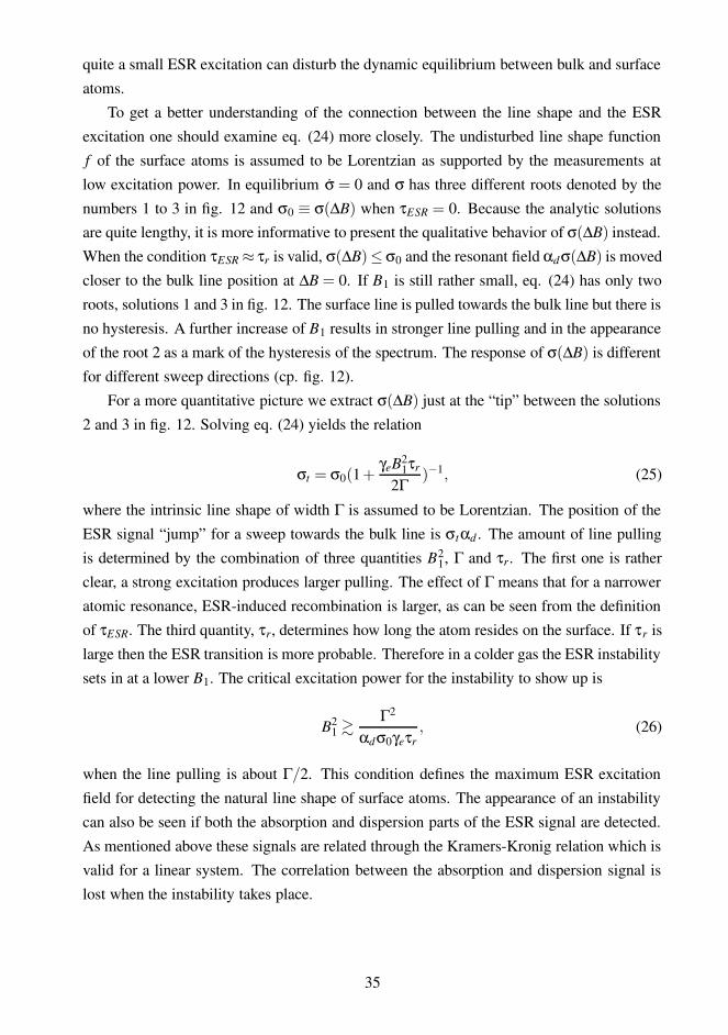
Figure 13: ESR line shapes of 2D H with σ = 1012 cm−2 and Tliq = 78 mK measured inSCII. The two lower lines are distorted by the applied radial magnetic field gradients equalin amplitude but opposite in polarity. The uppermost line is measured without gradient andthe dashed line is a fitted Lorentzian function.

3.1.2 Line broadening due to magnetic field inhomogeneities

Next we consider the inhomogeneity of the magnetic field and the frequency instability of

the mm-wave source (MWS) as the origin for the ESR line broadening in the limit of small

excitation power. The field inhomogeneity can originate from that of the external magnetic

field and from the internal dipolar field which is inhomogeneous due to the uneven density

distribution of H atoms adsorbed on the cold spot. These do not only contribute to the

linewidth but also make the line asymmetric. The surface ESR line shape is described by

eq. (23), where according to eq. (22) the line shape function f is a convolution of the

intrinsic line shape and the frequency spectrum of the MWS. We found that the width of

the MWS spectrum depended on the operating frequency: In some experimental runs its

contribution to the linewidth was discernible but in most cases insignificantly small.

In comparison to the bulk line, the surface line is sensitive only to radial gradients of

the magnetic field. The gradients are caused by field inhomogeneities of the main magnet

and the ESR sweep coil and by the various magnetization of materials in the vicinity of

the CS. An uneven density distribution also leads to an inhomogeneous intrinsic dipolar

field αdσ(r) over the cold spot. Changes in temperature, flow of atoms on the surface, and

36

0 1 2 3 4

Surface density [1012cm-2]

0.1

0.2

0.3

0.4

0.5

Surf

ace

linew

idth

[G]

Tb = 178 mKTb = 138 mK

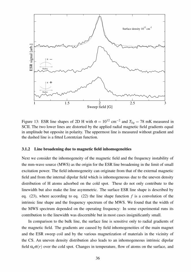
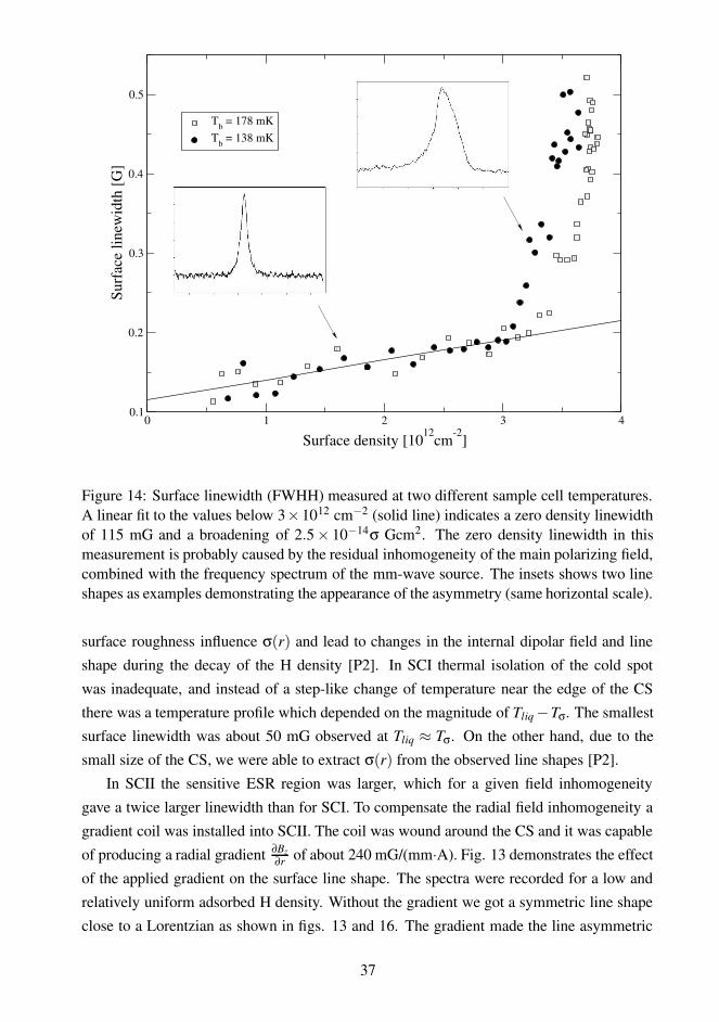
Figure 14: Surface linewidth (FWHH) measured at two different sample cell temperatures.A linear fit to the values below 3×1012 cm−2 (solid line) indicates a zero density linewidthof 115 mG and a broadening of 2.5× 10−14σ Gcm2. The zero density linewidth in thismeasurement is probably caused by the residual inhomogeneity of the main polarizing field,combined with the frequency spectrum of the mm-wave source. The insets shows two lineshapes as examples demonstrating the appearance of the asymmetry (same horizontal scale).

surface roughness influence σ(r) and lead to changes in the internal dipolar field and line

shape during the decay of the H density [P2]. In SCI thermal isolation of the cold spot

was inadequate, and instead of a step-like change of temperature near the edge of the CS

there was a temperature profile which depended on the magnitude of Tliq −Tσ. The smallestsurface linewidth was about 50 mG observed at Tliq ≈ Tσ. On the other hand, due to the

small size of the CS, we were able to extract σ(r) from the observed line shapes [P2].

In SCII the sensitive ESR region was larger, which for a given field inhomogeneity

gave a twice larger linewidth than for SCI. To compensate the radial field inhomogeneity a

gradient coil was installed into SCII. The coil was wound around the CS and it was capable

of producing a radial gradient ∂Bz∂r of about 240 mG/(mm·A). Fig. 13 demonstrates the effect

of the applied gradient on the surface line shape. The spectra were recorded for a low and

relatively uniform adsorbed H density. Without the gradient we got a symmetric line shape

close to a Lorentzian as shown in figs. 13 and 16. The gradient made the line asymmetric

37

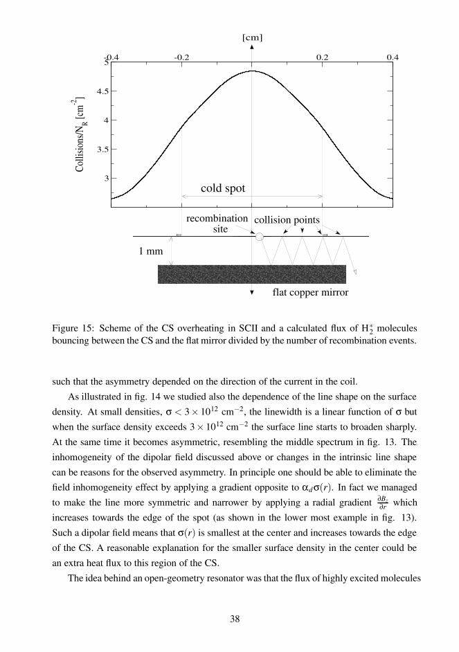
-0.4 -0.2 0 0.2 0.4

[cm]

3

3.5

4

4.5

5

Colli

sions

/NR [c

m-2

]

cold spot

flat copper mirror

siterecombination collision points

1 mm

Figure 15: Scheme of the CS overheating in SCII and a calculated flux of H∗2 molecules

bouncing between the CS and the flat mirror divided by the number of recombination events.

such that the asymmetry depended on the direction of the current in the coil.

As illustrated in fig. 14 we studied also the dependence of the line shape on the surface

density. At small densities, σ < 3× 1012 cm−2, the linewidth is a linear function of σ but

when the surface density exceeds 3× 1012 cm−2 the surface line starts to broaden sharply.

At the same time it becomes asymmetric, resembling the middle spectrum in fig. 13. The

inhomogeneity of the dipolar field discussed above or changes in the intrinsic line shape

can be reasons for the observed asymmetry. In principle one should be able to eliminate thefield inhomogeneity effect by applying a gradient opposite to αdσ(r). In fact we managed

to make the line more symmetric and narrower by applying a radial gradient ∂Bz∂r which

increases towards the edge of the spot (as shown in the lower most example in fig. 13).

Such a dipolar field means that σ(r) is smallest at the center and increases towards the edge

of the CS. A reasonable explanation for the smaller surface density in the center could be

an extra heat flux to this region of the CS.

The idea behind an open-geometry resonator was that the flux of highly excited molecules

38

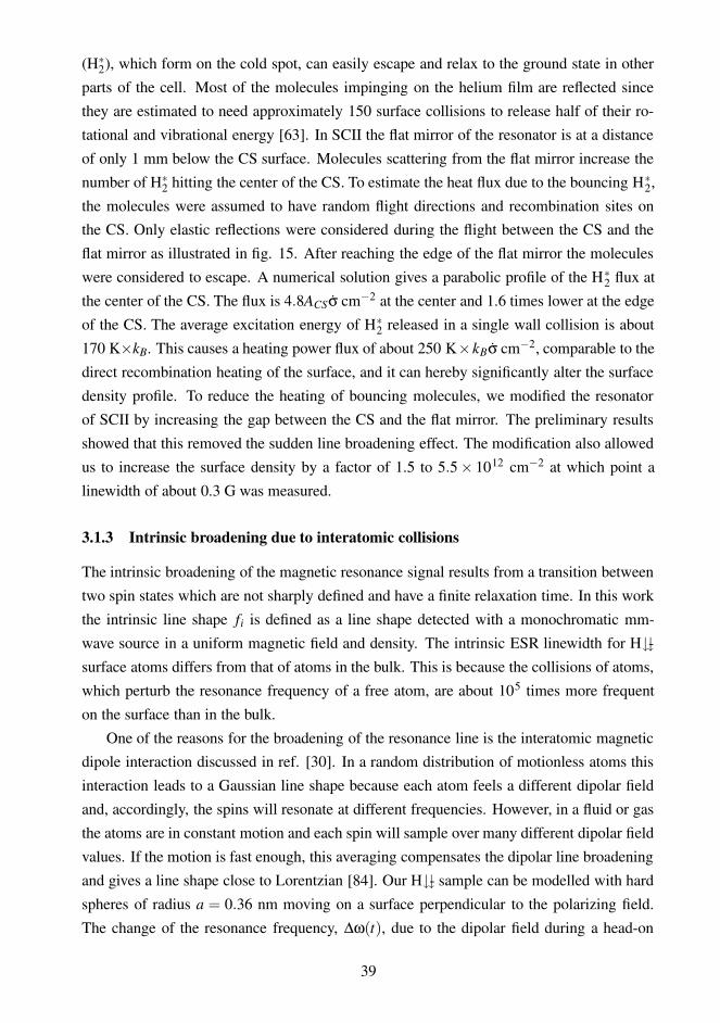
(H∗2), which form on the cold spot, can easily escape and relax to the ground state in other

parts of the cell. Most of the molecules impinging on the helium film are reflected since

they are estimated to need approximately 150 surface collisions to release half of their ro-

tational and vibrational energy [63]. In SCII the flat mirror of the resonator is at a distance

of only 1 mm below the CS surface. Molecules scattering from the flat mirror increase the

number of H∗2 hitting the center of the CS. To estimate the heat flux due to the bouncing H∗

2,

the molecules were assumed to have random flight directions and recombination sites onthe CS. Only elastic reflections were considered during the flight between the CS and the

flat mirror as illustrated in fig. 15. After reaching the edge of the flat mirror the molecules

were considered to escape. A numerical solution gives a parabolic profile of the H∗2 flux at

the center of the CS. The flux is 4.8ACSσ cm−2 at the center and 1.6 times lower at the edge

of the CS. The average excitation energy of H∗2 released in a single wall collision is about

170 K×kB. This causes a heating power flux of about 250 K×kBσ cm−2, comparable to the

direct recombination heating of the surface, and it can hereby significantly alter the surface

density profile. To reduce the heating of bouncing molecules, we modified the resonator

of SCII by increasing the gap between the CS and the flat mirror. The preliminary results

showed that this removed the sudden line broadening effect. The modification also allowed

us to increase the surface density by a factor of 1.5 to 5.5× 1012 cm−2 at which point a

linewidth of about 0.3 G was measured.

3.1.3 Intrinsic broadening due to interatomic collisions

The intrinsic broadening of the magnetic resonance signal results from a transition between

two spin states which are not sharply defined and have a finite relaxation time. In this work

the intrinsic line shape fi is defined as a line shape detected with a monochromatic mm-

wave source in a uniform magnetic field and density. The intrinsic ESR linewidth for H�-

surface atoms differs from that of atoms in the bulk. This is because the collisions of atoms,

which perturb the resonance frequency of a free atom, are about 105 times more frequent

on the surface than in the bulk.

One of the reasons for the broadening of the resonance line is the interatomic magneticdipole interaction discussed in ref. [30]. In a random distribution of motionless atoms this

interaction leads to a Gaussian line shape because each atom feels a different dipolar field

and, accordingly, the spins will resonate at different frequencies. However, in a fluid or gas

the atoms are in constant motion and each spin will sample over many different dipolar field

values. If the motion is fast enough, this averaging compensates the dipolar line broadening

and gives a line shape close to Lorentzian [84]. Our H�- sample can be modelled with hard

spheres of radius a = 0.36 nm moving on a surface perpendicular to the polarizing field.

The change of the resonance frequency, ∆ω(t), due to the dipolar field during a head-on

39

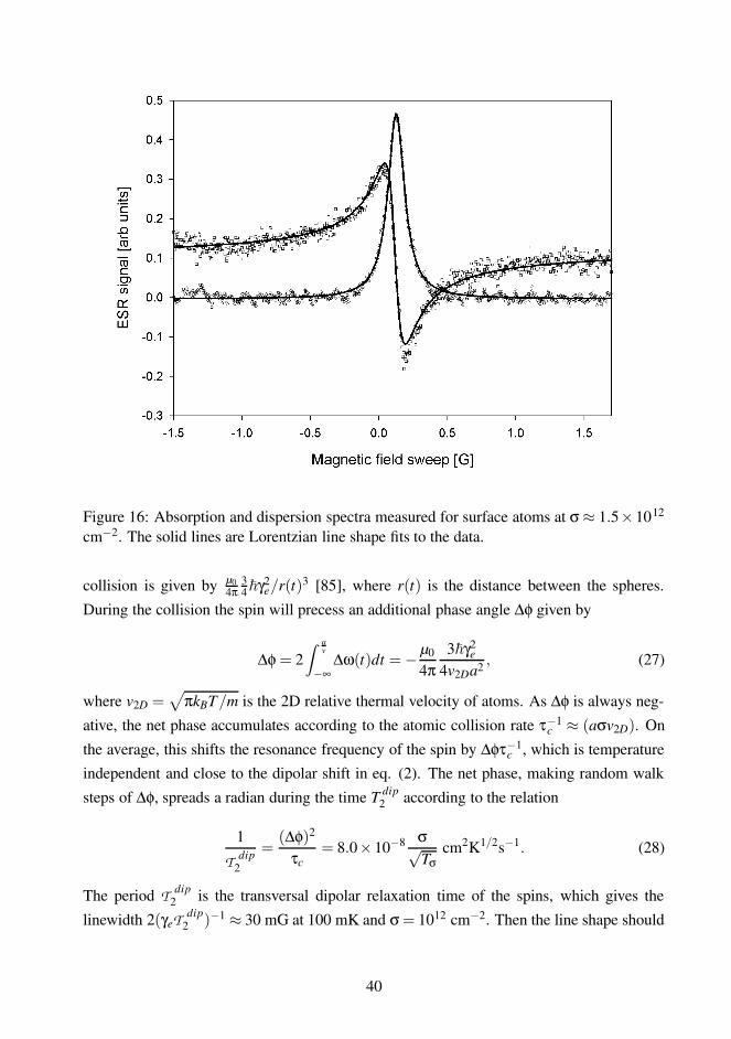
Figure 16: Absorption and dispersion spectra measured for surface atoms at σ ≈ 1.5×1012

cm−2. The solid lines are Lorentzian line shape fits to the data.

collision is given by µ04π

34~γ2

e/r(t)3 [85], where r(t) is the distance between the spheres.

During the collision the spin will precess an additional phase angle ∆φ given by

∆φ = 2Z a

v

−∞∆ω(t)dt = − µ0

4π3~γ2

e

4v2Da2 , (27)

where v2D =√

πkBT/m is the 2D relative thermal velocity of atoms. As ∆φ is always neg-

ative, the net phase accumulates according to the atomic collision rate τ−1c ≈ (aσv2D). On

the average, this shifts the resonance frequency of the spin by ∆φτ−1c , which is temperature

independent and close to the dipolar shift in eq. (2). The net phase, making random walk

steps of ∆φ, spreads a radian during the time T dip2 according to the relation

1

T dip2

=(∆φ)2

τc= 8.0×10−8 σ√

Tσcm2K1/2s−1. (28)

The period T dip2 is the transversal dipolar relaxation time of the spins, which gives the

linewidth 2(γeT dip2 )−1 ≈ 30 mG at 100 mK and σ = 1012 cm−2. Then the line shape should

40

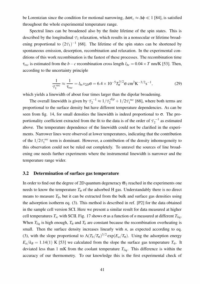
be Lorentzian since the condition for motional narrowing, ∆ωτc ≈ ∆φ � 1 [84], is satisfied

throughout the whole experimental temperature range.

Spectral lines can be broadened also by the finite lifetime of the spin states. This is

described by the longitudinal T1 relaxation, which results in a nonsecular or lifetime broad-

ening proportional to (2T1)−1 [68]. The lifetime of the spin states can be shortened by

spontaneous emission, desorption, recombination and relaxation. In the experimental con-

ditions of this work recombination is the fastest of these processes. The recombination timeτrec is estimated from the b−c recombination cross length lbc = 0.04×T nm/K [53]. Then,

according to the uncertainty principle

1T rec

1≈ 1

τrec= lbcv2Dσ = 6.4×10−5T 3/2

σ σ cm2K−3/2s−1, (29)

which yields a linewidth of about four times larger than the dipolar broadening.

The overall linewidth is given by T −12 ≈ 1/T dip

2 +1/2T rec1 [68], where both terms are

proportional to the surface density but have different temperature dependencies. As can be

seen from fig. 14, for small densities the linewidth is indeed proportional to σ. The pro-

portionality coefficient extracted from the fit to the data is of the order of T −12 as estimated

above. The temperature dependence of the linewidth could not be clarified in the experi-

ments. Narrower lines were observed at lower temperatures, indicating that the contribution

of the 1/2T rec1 term is dominant. However, a contribution of the density inhomogeneity to

this observation could not be ruled out completely. To unravel the sources of line broad-

ening one needs further experiments where the instrumental linewidth is narrower and the

temperature range wider.

3.2 Determination of surface gas temperature

In order to find out the degree of 2D quantum degeneracy ϖ2 reached in the experiments one

needs to know the temperature Tσ of the adsorbed H gas. Understandably there is no direct

means to measure Tσ, but it can be extracted from the bulk and surface gas densities using

the adsorption isotherm eq. (3). This method is described in ref. [P2] for the data obtained

in the sample cell version SCI. Here we present a similar result for data measured at higher

cell temperatures Tsc with SCII. Fig. 17 shows σ as a function of n measured at different Tliq.

When Tliq is high enough, Tσ and Tb are constant because the recombination overheating is

small. Then the surface density increases linearly with n, as expected according to eq.

(3), with the slope proportional to Λ(Tb/Tσ)3/2 exp(Ea/Tσ). Using the adsorption energy

Ea/kB = 1.14(1) K [53] we calculated from the slope the surface gas temperature Tσ. It

deviated less than 1 mK from the coolant temperature Tliq. This difference is within the

accuracy of our thermometry. To our knowledge this is the first experimental check of

41

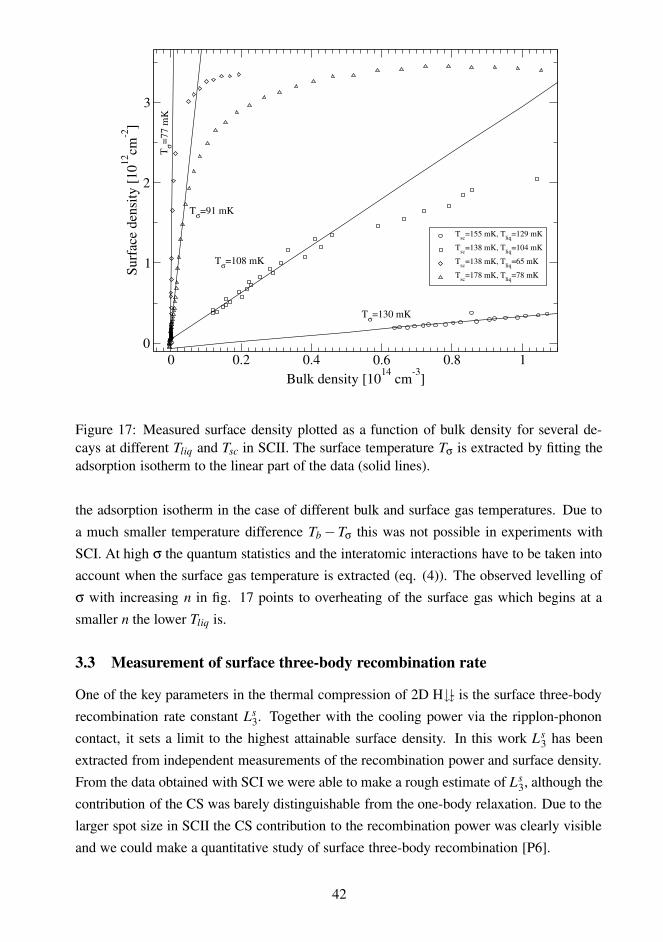
0 0.2 0.4 0.6 0.8 1Bulk density [1014 cm-3]

0

1

2

3

Surf

ace

dens

ity [1

012cm

-2]

Tsc=155 mK, Tliq=129 mK

Tsc=138 mK, Tliq=104 mK

Tsc=138 mK, Tliq=65 mK

Tsc=178 mK, Tliq=78 mK

Tσ=130 mK

Tσ=108 mK

Tσ=91 mK

Tσ=7

7 m

K

Figure 17: Measured surface density plotted as a function of bulk density for several de-cays at different Tliq and Tsc in SCII. The surface temperature Tσ is extracted by fitting theadsorption isotherm to the linear part of the data (solid lines).

the adsorption isotherm in the case of different bulk and surface gas temperatures. Due to

a much smaller temperature difference Tb −Tσ this was not possible in experiments with

SCI. At high σ the quantum statistics and the interatomic interactions have to be taken into

account when the surface gas temperature is extracted (eq. (4)). The observed levelling of

σ with increasing n in fig. 17 points to overheating of the surface gas which begins at a

smaller n the lower Tliq is.

3.3 Measurement of surface three-body recombination rate

One of the key parameters in the thermal compression of 2D H�- is the surface three-body

recombination rate constant Ls3. Together with the cooling power via the ripplon-phonon

contact, it sets a limit to the highest attainable surface density. In this work Ls3 has been

extracted from independent measurements of the recombination power and surface density.

From the data obtained with SCI we were able to make a rough estimate of Ls3, although the

contribution of the CS was barely distinguishable from the one-body relaxation. Due to the

larger spot size in SCII the CS contribution to the recombination power was clearly visible

and we could make a quantitative study of surface three-body recombination [P6].

42

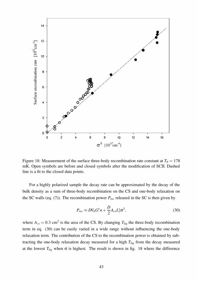
Figure 18: Measurement of the surface three-body recombination rate constant at Tb = 178mK. Open symbols are before and closed symbols after the modification of SCII. Dashedline is a fit to the closed data points.

For a highly polarized sample the decay rate can be approximated by the decay of the

bulk density as a sum of three-body recombination on the CS and one-body relaxation on

the SC walls (eq. (7)). The recombination power Prec released in the SC is then given by

Prec ≈ DVhGen+D2

AcsLs3σ3, (30)

where Acs = 0.3 cm2 is the area of the CS. By changing Tliq the three-body recombination

term in eq. (30) can be easily varied in a wide range without influencing the one-body

relaxation term. The contribution of the CS to the recombination power is obtained by sub-

tracting the one-body relaxation decay measured for a high Tliq from the decay measured

at the lowest Tliq when σ is highest. The result is shown in fig. 18 where the difference

43

2(Prec −DVhGen)/D is plotted as a function of the third power of the surface density. The

open and closed symbols refer to measurements, respectively, before and after the modifi-

cations of the sample cell SCII.

The upward trend of the open-symbol data for σ & 3× 1012 cm−2 in fig. 18 begins

at the same surface density where the ESR line shape starts to become asymmetric. This

feature may be accounted for by the overheating of the CS center by excited H2 molecules

bouncing from the flat mirror, as discussed in section 3.1.2. The ESR signal originates fromatoms near the CS center only. In the case of the overheating the detected σ is therefore

lower than the average σ on the CS and the corresponding data points in fig. 18 are shifted

towards lower σ. The value Ls3 = 2(1)×1025 cm4s−1 [P6] is extracted from the data points

which follow a linear dependence in fig. 18. The data measured after the cell modifica-

tions is entirely linear and up to the highest densities consistent with the above-mentioned

Ls3 value. The results obtained for Ls

3 in different experimental runs of the present work at

temperatures between 85 and 130 mK are reproducible but approximately 10 times smaller

than the previously reported values (cp. e.g. refs. [51, 52, 79]). A possible explanation for

this large deviation could be the indirect determination of the surface density and recombi-

nation power in earlier measurements. This important issue is discussed in more detail in

papers [P2] and [P6].

Theoretical studies of the surface three-body recombination were performed by Kagan

et al. [36] and de Goey et al. [62]. Due to the absence of exchange interaction in mutual

collisions of b-state atoms the dipole mechanism is the only efficient recombination process

which was discussed by both of these theory groups. Kagan et al. used a simplified approach

where the surface rate constant was calculated from the bulk rate constant by scaling the

latter to the surface using the relation Ls3 ≈ Lb

3/l2d . De Goey et al. took the delocalization

more accurately into account, and obtained Ls3 = 1.3×10−25 cm4s−1 at 4.6 T which is more

than an order of magnitude smaller than the value reported by Kagan et al. [36]. Compared

to our experimental result de Goey’s calculation is within the error bar, which brings down

the long-term discrepancy between theoretical and experimental values of Ls3.

3.4 Limits of thermal compression

In this work the highest surface density observed was about 5.5× 1012 cm−2 at Tσ ≈ 110

mK, corresponding to the 2D phase-space density ϖ2 ≈ 1.6. The dense surface gas was

overheated well above the coolant temperature and σ was almost independent of the bulk

gas density as shown in fig. 17. The main source of heat was caused directly by recom-

bination of the surface gas. Neglecting other sources of heat except the three-body surface

recombination, a simple equation for the maximum quantum degeneracy ϖ2 on the CS can

be derived. The recombination heat absorbed by the surface of the cold spot is given by

44

P3b = ( f +(1− f )Acs

Ac)D2

Ls3σ3, (31)

where Ac is the area of the sample cell, and f is the fraction of the heat dumped directly

to the cold spot surface ( f ≤ 2 % [26, 63, 65]). The efficiency with which this heat can be

removed is defined by the ripplon-phonon thermal contact (eq. (5)). Setting P3b = Prp we

get an estimate of the highest achievable quantum degeneracy as

ϖ2 ≡ σΛ2 =2π~

2

mkB3

√

2Grp

DL3( f +(1− f )ACSAC

)T

119

σ ≈ 22T119

σ . (32)

In fig. 19 we present the highest ϖ2 data obtained in SCII together with plots of the ad-

sorption isotherm at several surface temperatures. Two sets of data are plotted, one takenbefore and the other after the improvement of the H∗

2 escape from the CS, as described in

section 3.1.2. The result of the improvement can be clearly seen as a factor of 1.5 increase

in the surface density. Eq. (32), together with the adsorption isotherm (3), implicitly de-

fines the maximum surface density σ(n), which can be reached for a given bulk density n

and temperature Tb. For Tb = 178 mK we plot σ(n) in fig. 19 as the dotted line. The dashed

line marks the condition of quasi-condensate formation ϖ2 = 3 [20]. We include an abrupt

change of the interactions in 2D gas, taken into account by the two-body correlator g2 in eq.

(4), which leads to an increase of σ by a factor of two in the quasi-condensate [46].

Eq. (5) predicts that in order to increase ϖ2 one has to use higher Tσ. One can estimate

that the condition ϖ2 ≈ 3 required for quasi-condensate formation can be reached at Tσ ≈200 mK and n ≈ 1017 cm−3, found as a crossing of the dashed and dotted lines in fig. 19.

The use of such a high bulk density would increase the heating of the surface due to the

thermal accommodation,

Pacc =nv3s

42kB(Tb −Tσ). (33)

The heating Pacc becomes comparable with the surface three-body recombination heating

if the temperature difference exceeds 100 mK at n = 6× 1016 cm−3. Therefore, a further

increase of n does not help to reach a higher degeneracy of the surface gas. On the other

hand, from the experimental data of fig. 19 it is evident that only a twofold increase of σwould be needed. Some increase of ϖ2 may be possible by a further improvement of the

escape of H∗2. This can be done by making the cell more open by using e.g. a coarse grid

as a mirror below the spot. Another way to work is to increase the adsorption energy. This

can be done by utilizing a thin unsaturated helium film [49] at the CS. The thinner film

will possibly reduce the value of Ls3 [P6] and increase the ripplon-phonon thermal contact.

Making a superfluid helium film locally thinner is, however, a difficult technical problem

45

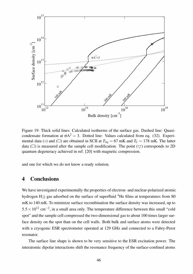
1012 10141016 1018

Bulk density [cm-3]

1011

1012

1013

1014

1015

Surf

ace

dens

ity [c

m-2

]

100 m

K

200 m

K

300 m

K

σΛ2=3

Figure 19: Thick solid lines: Calculated isotherms of the surface gas. Dashed line: Quasi-condensate formation at σΛ2 = 3. Dotted line: Values calculated from eq. (32). Experi-mental data (◦) and (�) are obtained in SCII at Tliq = 67 mK and TC = 178 mK. The latterdata (�) is measured after the sample cell modification. The point (5) corresponds to 2Dquantum degeneracy achieved in ref. [20] with magnetic compression.

and one for which we do not know a ready solution.

4 Conclusions

We have investigated experimentally the properties of electron- and nuclear-polarized atomic

hydrogen H�- gas adsorbed on the surface of superfluid 4He films at temperatures from 80

mK to 140 mK. To minimize surface recombination the surface density was increased, up to

5.5×1012 cm−2, in a small area only. The temperature difference between this small “cold

spot” and the sample cell compressed the two-dimensional gas to about 100 times larger sur-

face density on the spot than on the cell walls. Both bulk and surface atoms were detected

with a cryogenic ESR spectrometer operated at 129 GHz and connected to a Fabry-Perot

resonator.

The surface line shape is shown to be very sensitive to the ESR excitation power. The

interatomic dipolar interactions shift the resonance frequency of the surface-confined atoms

46

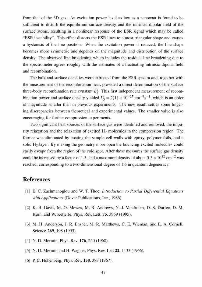
from that of the 3D gas. An excitation power level as low as a nanowatt is found to be

sufficient to disturb the equilibrium surface density and the intrinsic dipolar field of the

surface atoms, resulting in a nonlinear response of the ESR signal which may be called

“ESR instability”. This effect distorts the ESR lines to almost triangular shape and causes

a hysteresis of the line position. When the excitation power is reduced, the line shape

becomes more symmetric and depends on the magnitude and distribution of the surface

density. The observed line broadening which includes the residual line broadening due tothe spectrometer agrees roughly with the estimates of a fluctuating intrinsic dipolar field

and recombination.

The bulk and surface densities were extracted from the ESR spectra and, together with

the measurement of the recombination heat, provided a direct determination of the surface

three-body recombination rate constant Ls3. This first independent measurement of recom-

bination power and surface density yielded Ls3 = 2(1)× 10−25 cm−4s−1, which is an order

of magnitude smaller than in previous experiments. The new result settles some linger-

ing discrepancies between theoretical and experimental values. The smaller value is also

encouraging for further compression experiments.

Two significant heat sources of the surface gas were identified and removed, the impu-

rity relaxation and the relaxation of excited H2 molecules in the compression region. The

former was eliminated by coating the sample cell walls with epoxy, polymer foils, and a

solid H2 layer. By making the geometry more open the bouncing excited molecules could

easily escape from the region of the cold spot. After these measures the surface gas density

could be increased by a factor of 1.5, and a maximum density of about 5.5×1012 cm−2 was

reached, corresponding to a two-dimensional degree of 1.6 in quantum degeneracy.

References

[1] E. C. Zachmanoglou and W. T. Thoe, Introduction to Partial Differential Equations

with Applications (Dover Publications, Inc., 1986).

[2] K. B. Davis, M. O. Mewes, M. R. Andrews, N. J. Vandruten, D. S. Durfee, D. M.

Kurn, and W. Ketterle, Phys. Rev. Lett. 75, 3969 (1995).

[3] M. H. Anderson, J. R. Ensher, M. R. Matthews, C. E. Wieman, and E. A. Cornell,

Science 269, 198 (1995).

[4] N. D. Mermin, Phys. Rev. 176, 250 (1968).

[5] N. D. Mermin and H. Wagner, Phys. Rev. Lett 22, 1133 (1966).

[6] P. C. Hohenberg, Phys. Rev. 158, 383 (1967).

47

[7] V. L. Berezinskii, Sov. Phys. JETP 32, 493 (1971).

[8] J. M. Kosterlitz and D. J. Thouless, Two-dimensional physics, in Progress in low tem-

perature physics, edited by D. F. Brewer (North-Holland, 1978), vol. VIIb, p. 374.

[9] M. Bijlsma, Quantum degeneracy in a Bose gas, Ph.D. thesis, Eindhoven University

of Technology, Netherlands (1997).

[10] D. J. Bishop and J. D. Reppy, Phys. Rev. Lett 40, 1727 (1978).

[11] V. N. Popov, Functional integrals in quantum field theory and statistical physics (Rei-

del, Dordrecht, 1983).

[12] D. S. Petrov, D. M. Gangardt, and G. V. Shlyapnikov, Low-dimensional trapped gases,

in Journal de Physique IV , edited by L. Pricoupenko, H. Perrin, and M. Olshanii (EDP

Sciences, 2004), vol. 116, p. 3.

[13] M. Bijlsma and H. T. C. Stoof, Phys. Rev. E 47, 939 (1993).

[14] J. O. Andersen, U. Al Khawaja, and H. T. C. Stoof, Phys. Rev. Lett 88, 070407 (2002).

[15] U. Al Khawaja, J. O. Andersen, N. P. Proukakis, and H. T. C. Stoof, Phys. Rev. A 66,

013615 (2002).

[16] Yu. Kagan, V. A. Kashurnikov, A. V. Krasavin, N. V. Prokof’ev, and B. V. Svistunov,

Phys. Rev. A 61, 043608 (2000).

[17] N. Prokofev and B. Svistunov, Phys. Rev. A 66, 043608 (2002).

[18] I. F. Silvera and J. T. M. Walraven, Phys. Rev. Lett 44, 164 (1980).

[19] D. G. Fried, T. C. Killian, L. Willmann, D. Landhuis, S. C. Moss, D. Kleppner, and

T. J. Greytak, Phys. Rev. Lett 81, 3811 (1998).

[20] A. I. Safonov, S. A. Vasilyev, I. S. Yasnikov, I. I. Lukashevich, and S. Jaakkola, Phys.

Rev. Lett 81, 4545 (1998).

[21] M. Greiner, I. Bloch, O. Mandel, T. W. Hänsch, and T. Esslinger, Appl. Phys. B 73,

769 (2001).

[22] J. M. Görlitz, J. M. Vogels, A. E. Leanhardt, C. Raman, T. L. Gustavson, J. R. Abo-

Shaeer, A. P. Chikkatur, S. Gupta, S. Inouye, T. Rosenband, and W. Ketterle, Phys.Rev. Lett 87, 130402 (2001).

48

[23] M. Hammes, D. Rychtarik, B. Enseger, H.-C. Nägerl, and R. Grimm, Phys. Rev. Lett

90, 173001 (2003).

[24] S. Dettmer, D. Hellweg, P. Ryytty, J. J. Arlt, W. Ertmer, K. Sengstock, D. S. Petrov,

G. V. Shlyapnikov, H. Kreutzmann, L. Santos, and M. Lewenstein, Phys. Rev. Lett 87,

160406 (2001).

[25] S. Stock, Z. Hadzibabic, B. Battelier, M. Cheneau, and J. Dalibard, Phys. Rev. Lett 95,

190403 (2005).

[26] A. Matsubara, T. Arai, S. Hotta, J. S. Korhonen, T. Suzuki, A. Masaike, J. T. M.

Walraven, T. Mizusaki, and A. Hirai, Physica B 194, 899 (1994).

[27] S. Gupta, Z. Hadzibabic, M. W. Zwierlein, C. A. Stan, K. Dieckmann, C. H. Schunck,

E. G. M. Van Kempen, B. J. Verhaar, and W. Ketterle, Science 300, 1723 (2003).

[28] D. M. Harber, H. J. Lewandowski, J. M. Mcguirk, and E. A. Cornell, Phys. Rev. A 66,

053616 (2002).

[29] M. W. Zwierlein, Z. Hadzibabic, S. Gupta, and W. Ketterle, Phys. Rev. Lett 91, 250404

(2003).

[30] I. Shinkoda and W. N. Hardy, J. Low Temp. Phys. 85, 99 (1991).

[31] W. Kolos and L. Wolniewicz, J. Chem. Phys. 43, 2429 (1965).

[32] W. Kolos and L. Wolniewicz, Chem. Phys. Lett. 24, 457 (1974).

[33] C. E. Hecht, Physica 25, 1159 (1959).

[34] I. F. Silvera and J. T. M. Walraven, Spin-polarized atomic hydrogen, in Progress in

Low Temperature Physics, edited by D. F. Brewer (North-Holland, Amsterdam, 1986),

vol. X, p. 139.

[35] Y. P. Zhang, C. H. Cheng, J. T. Kim, J. Stanojevic, and E. E. Eyler, Phys. Rev. Lett 92,203003 (2004).

[36] Yu. Kagan, I. A. Vartanyants, and G. V. Shlyapnikov, Sov. Phys. JETP 54, 590 (1981).

[37] J. M. Greben, A. W. Thomas, and A. J. Berlinsky, Can. J. Phys. 59, 945 (1981).

[38] L. P. H. De Goey, J. P. J. Driessen, Verhaar B. J., and J. T. M. Walraven, Phys. Rev.Lett 53, 1919 (1984).

49

[39] M. W. Reynolds, I. Shinkoda, W. N. Hardy, A. J. Berlinsky, F. Bridges, and B. W.

Statt, Phys. Rev. B 31, 7503 (1985).

[40] R. A. Guyer and M. D. Miller, Phys. Rev. Lett 42, 1754 (1979).

[41] I. B. Mantz and D. O. Edwards, Phys. Rev. B 20, 4518 (1979).

[42] D. O. Edwards and W. F. Saam, The free surface of liquid helium, in Progress in Low

Temperature Physics, edited by D. F. Brewer (North-Holland, Amsterdam, 1978), vol.

VII A, p. 283.

[43] J. T. M. Walraven, Atomic hydrogen and liquid helium surfaces, in Fundamental sys-

tems in quantum optics, edited by J. Dalibard, J. M. Raimond, and J. Zinn-Justin

(Elsevier Science Publishers, Amsterdam, 1992), p. 487.

[44] H. Gauck, M. Hartl, D. Schneble, H. Schnitzler, T. Pfau, and J. Mlynek, Phys. Rev.

Lett 81, 5298 (1998).

[45] E. A. Hinds, M. G. Boshier, and I. G. Hughes, Phys. Rev. Lett 80, 645 (1998).

[46] B. V. Svistunov, T. M. Hijmans, G. V. Shlyapnikov, and J. T. M. Walraven, Phys. Rev.

B 43, 13412 (1991).

[47] J. J. Berkhout and J. T. M. Walraven, Phys. Rev. B 47, 8886 (1993).

[48] I. A. Yu, J. M. Doyle, J. C. Sandberg, C. L. Cesar, D. Kleppner, and T. J. Greytak,

Phys. Rev. Lett. 71, 1589 (1993).

[49] H. P. Godfried, E. R. Eliel, J. G. Brisson, J. D. Gillaspy, C. Mallardeau, J. C. Mester,

and I. F. Silvera, Phys. Rev. Lett 55, 1311 (1985).

[50] M. Morrow, R. Jochemsen, A. J. Berlinsky, and W. N. Hardy, Phys. Rev. Lett 47, 455

(1981).

[51] D. A. Bell, H. F. Hess, G. P. Kochanski, S. Buchman, L. Pollack, Y. M. Xiao, D. Klepp-ner, and T. J. Greytak, Phys. Rev. B 34, 7670 (1986).

[52] R. Sprik, J. T. M. Walraven, G. H. Van Yperen, and I. F. Silvera, Phys. Rev. B 34, 6172

(1986).

[53] A. I. Safonov, S. A. Vasiliev, A. A. Kharitonov, S. T. Boldarev, I. I. Lukashevich, and

S. Jaakkola, Phys. Rev. Lett 86, 3356 (2001).

[54] D. S. Zimmerman and A. J. Berlinsky, Can. J. Phys. 62, 590 (1984).

50

[55] M. W. Reynolds, I. D. Setija, and G. V. Shlyapnikov, Phys. Rev. B 46, 575 (1992).

[56] O. V. Lounasmaa, Experimental principles and methods below 1 K (Academic Press,

1974).

[57] M. D. Lee, S. A. Morgan, M. J. Davis, and K. Burnett, Phys. Rev. A 65, 043617

(2002).

[58] D. S. Petrov and G. V. Shlyapnikov, Phys. Rev. A 64, 012706 (2001).

[59] M. J. Jamieson, A. Dalgarno, and J. N. Yukich, Phys. Rev. A 46, 6956 (1992).

[60] Yu. Kagan, B. V. Svistunov, and G. V. Shlyapnikov, Sov. Phys. JETP 66, 314 (1987).

[61] D. S. Petrov, M. Holzmann, and G. V. Shlyapnikov, Phys. Rev. Lett 84, 2551 (2000).

[62] L. P. H. De Goey, H. T. C. Stoof, J. M. V. A. Koelman, B. J. Verhaar, and J. T. M.

Walraven, Phys. Rev. B 38, 11500 (1988).

[63] S. A. Vasiliev, E. Tjukanoff, M. Mertig, A. Ya. Katunin, and S. Jaakkola, Europhys.

Lett. 24, 223 (1993).

[64] A. Matsubara, T. Arai, S. Hotta, J. S. Korhonen, T. Suzuki, A. Masaike, J. T. M.

Walraven, T. Mizusaki, and A. Hirai, Physica B 194-196, 899 (1994).

[65] E. S. Meyer, Z. Zhao, J. C. Mester, and I. F. Silvera, Phys. Rev. B 50, 9339 (1994).

[66] E. A. Burt, R. W. Ghrist, C. J. Myatt, M. J. Holland, E. A. Cornell, and C. E. Wieman,

Phys. Rev. Lett 79, 337 (1997).

[67] Yu. Kagan, B. V. Svistunov, and G. V. Shlyapnikov, JETP Lett. 42, 208 (1985).

[68] C. P. Slichter, Principles of Magnetic Resonance (Springer-Verlag, Heidelberg, 1992),

third edn.

[69] B. W. Statt, W. N. Hardy, A. J. Berlinsky, and E. Klein, J. Low Temp. Phys. 61, 471

(1985).

[70] G. H. Van Yperen, J. T. M. Walraven, and I. F. Silvera, Phys. Rev. B 30, 2386 (1984).

[71] M. Mertig, E. Tjukanov, S. A. Vasilyev, A. Ya. Katunin, and S. Jaakkola, J. Low Temp.

Phys. 100, 45 (1995).

[72] B. Yurke, D. Igner, E. Smith, B. Johnson, J. Denker, C. Hammel, D. Lee, and J. Freed,

J. Phys-Paris (Colloq.) C7, 177 (1980).

51

[73] N. Bloembergen and R. V. Pound, Phys. Rev. 95, 8 (1954).

[74] C. P. Poole, Electron Spin Resonance (John Wiley and Sons, 1967).

[75] H. A. Haus, Waves and fields in optoelectronics (Prentise-Hall Inc., 1984), first edn.

[76] S. A. Vasiliev, A. Ya. Katunin, A. I. Safonov, A. V. Frolov, and E. Tjukanoff, Appl.

Magn. Reson. 3, 1061 (1992).

[77] R. Van Roijen, J. J. Berkhout, B. Hebral, and J. T. M. Walraven, A cryogenic dissoci-

ator for atomic hydrogen (1989). Universiteit van Amsterdam, unpublished.

[78] H. Kogelnik and T. Li, Proc. IEEE 54, 1312 (1966).

[79] H. F. Hess, D. A. Bell, G. P. Kochanski, D. Kleppner, and T. J. Greytak, Phys. Rev.

Lett. 52, 1520 (1984).

[80] B. W. Statt, A. J. Berlinsky, and W. N. Hardy, Phys. Rev. B 31, 3169 (1985).

[81] R. Sprik, J. T. M. Walraven, G. H. Van Yperen, and I. F. Silvera, Phys. Rev. Lett 49,

153 (1982).

[82] P. W. Anderson and H. Suhl, Phys. Rev. 100, 1788 (1955).

[83] B. Lax and K. J. Button, Microwave ferrites and ferrimagnets (McGraw-Hill, 1962).

[84] R. Kubo, M. Toda, and N. Hashitsume, Statistical physics II : Nonequilibrium statis-

tical mechanics (Springer-Verlag, 1985).

[85] C. P. Poole and H. A. Farach, Relaxation in magnetic resonance (Academic press,

1971).

52