Borrowing Strength from Experience: Empirical Bayes...

Borrowing Strength from Experience:Empirical Bayes Methods and Convex

Optimization

Ivan Mizera

University of AlbertaEdmonton, Alberta, Canada

Department of Mathematical and Statistical Sciences

(“Edmonton Eulers”)

Wien, January 2016

Research supported by theNatural Sciences and Engineering Research Council of Canada

co-authors: Roger Koenker (Illinois), Mu Lin, Sile Tao (Alberta)1

Compound decision problem

• Estimate (predict) a vector µ = (µ1, · · · ,µn)Many quantities here, and not that much of sample for those• Observing one Yi for every µi, with (conditionally) known

distributionExample: Yi ∼ Binomial(ni,µi), ni knownAnother example: Yi ∼ N(µi, 1)Yet another example: Yi ∼ Poisson(µi)• µi’s assumed to be sampled (→ random) iid-ly from P

Thus, when the conditional density (...) of the Yi’s is ϕ(y,µ),then the marginal density of the Yi’s is

g(y) =

∫ϕ(y,µ)dP(µ)

2

A sporty exampleData: known performance of individual players, typicallysummarized as of successes, ki, in a number, ni, of somerepeated trials (bats, penalties) - typically, data not veryextensive (start of the season, say); the objective is to predict“true” capabilities of individual players

One possibility: Yi = ki ∼ Binomial(ni,µi)

Another possibility: take Yi = arcsinki + 1/4ni + 1/2

∼ N

(µi,

14ni

)Solutions via maximum likelihood

µi = ki/ni or µi = µiThe overall mean (or marginal MLE) is often better than this

Efron and Morris (1975), Brown (2008),Koenker and Mizera (2014): bayesball

3

NBA data (Agresti, 2002)

player n k prop

1 Yao 13 10 0.7692

2 Frye 10 9 0.9000

3 Camby 15 10 0.6667

4 Okur 14 9 0.6429

5 Blount 6 4 0.6667

6 Mihm 10 9 0.9000 it may be better to take

7 Ilgauskas 10 6 0.6000 the overall mean!

8 Brown 4 4 1.0000

9 Curry 11 6 0.5455

10 Miller 10 9 0.9000

11 Haywood 8 4 0.5000

12 Olowokandi 9 8 0.8889

13 Mourning 9 7 0.7778

14 Wallace 8 5 0.6250

15 Ostertag 6 1 0.1667

4

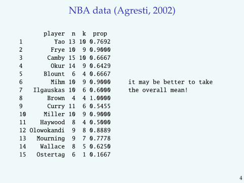
An insurance example

Yi - known number of accidents of individual insured motorists

Predict their expected number - rate, µi (in next year, say)

Yi ∼ Poisson(µi)

Maximum likelihood: µi = Yi

Nothing better?

5

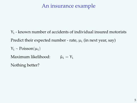
The data of Simar (1976)

6

So, what is better?

First, what is better?

We express it via some (expected) loss function

Most often it is averaged or aggregated squared error loss∑

i

(µi − µi)2

But it could be also some other loss...

And then?

Well, it is sooo simple...

7

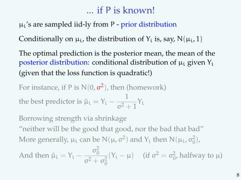
... if P is known!µi’s are sampled iid-ly from P - prior distribution

Conditionally on µi, the distribution of Yi is, say, N(µi, 1)

The optimal prediction is the posterior mean, the mean of theposterior distribution: conditional distribution of µi given Yi(given that the loss function is quadratic!)

For instance, if P is N(0,σ2), then (homework)

the best predictor is µi = Yi −1

σ2 + 1Yi

Borrowing strength via shrinkage“neither will be the good that good, nor the bad that bad”More generally, µi can be N(µ,σ2) and Yi then N(µi,σ2

0),

And then µi = Yi −σ2

0

σ2 + σ20(Yi − µ) (if σ2 = σ2

0, halfway to µ)

8

“If only all of them published posthumously...”

Thomas Bayes (1701–1761)

9

But do we know P (or σ2)?

“Hierarchical model”“Random effects”“Smoothing”“Empirical Bayes”

“no less Bayes than empirical Bayes”

“we know it is frequentist, but frequentists think it is Bayesian,so this is why we discuss it here”

Many inventors ...

10

What is mathematics?

Herbert Ellis Robbins (1915–2001)

11

On experience in statistical decision theory (1954)

Antonın Spacek (1911–1961)

12

I. J. Good (2000)

Alann Mathison Turing (1912–1954)

13

So, how

A. we may try to estimate the prior - “f-modeling”, Efron (2014)B. or more directly, the prediction rule - “g-modeling”

A’. Estimated normal prior (parametric)(Nonparametric ouverture)

A. Empirical prior (nonparametric)B. Empirical prediction rule (nonparametric)Simulation contests

14

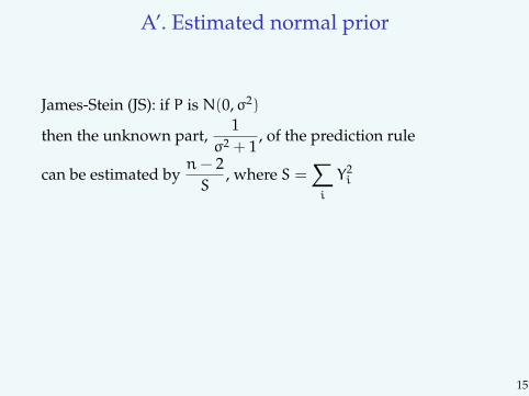
A’. Estimated normal prior

James-Stein (JS): if P is N(0,σ2)

then the unknown part,1

σ2 + 1, of the prediction rule

can be estimated byn− 2S

, where S =∑

i

Y2i

For general µ in place of 0, the rule is

µi = Yi −n− 3S

(Yi − Y), with Y =1n

∑

i

Yi and S =∑

i

(Yi − Y)2

15

JS as empirical Bayes: Efron and Morris (1975)

Charles Stein (1920– )

16

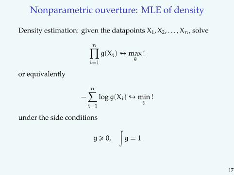
Nonparametric ouverture: MLE of density

Density estimation: given the datapoints X1,X2, . . . ,Xn, solve

n∏

i=1

g(Xi)# maxg

!

or equivalently

−

n∑

i=1

logg(Xi)# ming

!

under the side conditions

g > 0,∫g = 1

17

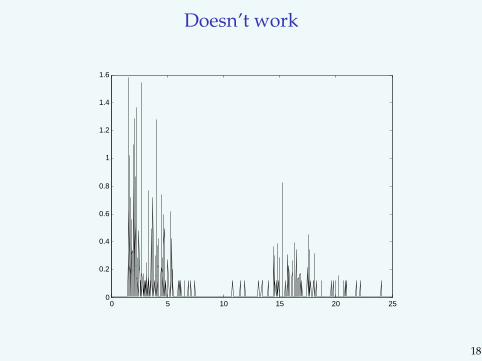
Doesn’t work

0 5 10 15 20 250

0.2

0.4

0.6

0.8

1

1.2

1.4

1.6

18

How to prevent Dirac catastrophe?

19

Reference

Koenker and Mizera (2014)... and those that cite it (Google Scholar)

“... the chance meeting on a dissecting-table of asewing-machine and an umbrella”

See also REBayes package on CRAN

For simplicity:ϕ(y,µ) = ϕ(y− µ), and the latter is standard normal density

20

A. Empirical prior

MLE of P: Kiefer and Wolfowitz (1956)

−∑

i

log(∫ϕ(Yi − u)dP(u)

)# min

P!

The regularizer is the fact that it is a mixtureNo tuning parameter needed (but “known” form of ϕ!)The resulting P is atomic (“empirical prior”)However, it is an infinite-dimensional problem...

21

EM nonsense

Laird (1978), Jiang and Zhang (2009):Use a grid {u1, ...um} (m = 1000)containing the support of the observed sampleand estimate the “prior density” via EM iterations

p(k+1)j =

1n

n∑

i=1

p(k)j ϕ(Yi − uj)

∑m`=1 p

(k)` ϕ(Yi − u`)

,

Sloooooow... (original versions: 55 hours for 1000 replications)

22

Convex optimization!

Koenker and Mizera (2014): it is a convex problem!

−∑

i


)# min

P!

When discretized

−∑

i

log

(∑m

ϕ(Yi − uj)pj

)# min

p!

or in a more technical form

−∑

i

logyi # miny

! Az = y and z ∈ S

where A = (ϕ(Yi − uj)) and S = {s ∈ Rm : 1>s = 1, s > 0}.

23

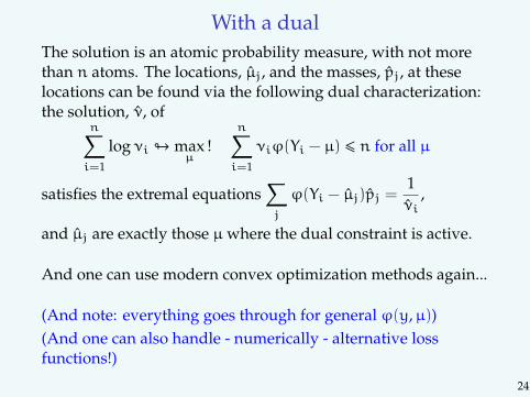
With a dualThe solution is an atomic probability measure, with not morethan n atoms. The locations, µj, and the masses, pj, at theselocations can be found via the following dual characterization:the solution, ν, of

n∑

i=1

logνi # maxµ

!n∑

i=1

νiϕ(Yi − µ) 6 n for all µ

satisfies the extremal equations∑

j

ϕ(Yi − µj)pj =1νi

,

and µj are exactly those µ where the dual constraint is active.

And one can use modern convex optimization methods again...

(And note: everything goes through for general ϕ(y,µ))(And one can also handle - numerically - alternative lossfunctions!)

24

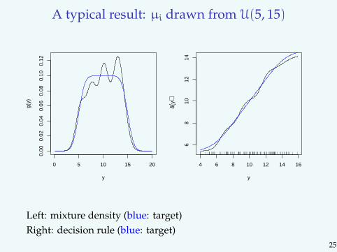
A typical result: µi drawn from U(5, 15)Koenker and Mizera 11

0 5 10 15 20

0.00

0.02

0.04

0.06

0.08

0.10

0.12

y

g(y)

4 6 8 10 12 14 16

68

1012

14

yδ(

y)

Figure 2. Estimated mixture density, g, and correspondingBayes rule, δ, for a simple compound decision problem. Thetarget Bayes rule and its mixture density are again plottedin dashed blue. In contrast to the shape constrained estima-tor shown in Figure 1, the Kiefer-Wolfowitz MLE employedfor this figure yields a much smoother and somewhat moreaccurate Bayes rule.

experiment. Each entry in the table is a sum of squared errors over the 1000observations, averaged over the number of replications. Johnstone andSilverman (2004) evaluated 18 different procedures; the last row of the tablereports the best performance, from the 18, achieved in their experimentfor each column setting. The performance of the Brown and Greenshtein(2009) kernel based rule is given in the fourth row of the table, taken fromtheir Table 1. Two variants of the GMLEB procedure of Jiang and Zhang(2009) appear in the second and third rows of the table. GMLEBEM isthe original proposal as implemented by Jiang and Zhang (2009) using100 iterations of the EM fixed point algorithm, GMLEBIP is the interiorpoint version iterated to convergence as determined by the Mosek defaults.The shape constrained estimator described above, denoted δ in the table,is reported in the first row. The δ and GMLEBIP results are based on1000 replications. The GMLEB results on 100 replications, the Brown andGreenshtein results on 50 replications, and the Johnstone and Silvermanresults on 100 replications, as reported in the respective original sources.

It seems fair to say that the shape constrained estimator performs com-petitively in all cases, but is particularly attractive relative to the kernelrule and the Johnstone and Silverman procedures in the moderate k and

Left: mixture density (blue: target)Right: decision rule (blue: target)

25

B. Empirical prediction rule

Lawrence Brown, personal communicationAlso, looks like in Maritz and Lwin (1989)Do not estimate P, but rather the prediction ruleTweedie formula: for known (general) P, and hence known g,the Bayes rule is

δ(y) = y+ σ2g′(y)g(y)

One may try to estimate g and plug it in - when knowing σ2

(=1, for instance)Brown and Greenshtein (2009)

by an exponential family argument, δ(y) is nondecreasing in y(van Houwelingen & Stijnen, 1983)(that came automatic when the prior is estimated)

26

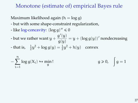
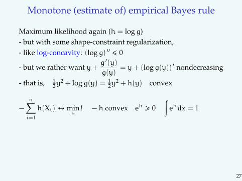
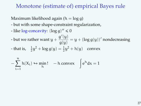
Monotone (estimate of) empirical Bayes rule

Maximum likelihood again (h = logg)- but with some shape-constraint regularization,- like log-concavity: (logg) ′′ 6 0

- but we rather want y+g ′(y)g(y)

= y+ (logg(y)) ′ nondecreasing

- that is, 12y

2 + logg(y) = 12y

2 + h(y) convex

−

n∑

i=1

logg(Xi)# ming

! g > 0,∫g = 1

The regularizer is the monotonicity constraintNo tuning parameter, or knowledge of ϕ

- but knowing all the time that σ2 = 1A convex problem again

27





- that is, 12y

2 + logg(y) = 12y

2 + h(y) convex

−

n∑

i=1

logg(Xi)# ming

! − logg convex g > 0∫gdx = 1



27





- that is, 12y

2 + logg(y) = 12y

2 + h(y) convex

−

n∑

i=1

h(Xi)# minh

! − h convex eh > 0∫

ehdx = 1



27





- that is, 12y

2 + logg(y) = 12y

2 + h(y) convex

−

n∑

i=1

h(Xi)# minh

! − h convex∫

ehdx = 1



27





- that is, 12y

2 + logg(y) = 12y

2 + h(y) convex

−

n∑

i=1

h(Xi) +

∫ehdx# min

h! − h convex



27





- that is, 12y

2 + logg(y) = 12y

2 + h(y) convex

−

n∑

i=1

h(Xi) +

∫ehdx# min

h!

12y2 + h(y) convex



27

Some remarks

After reparametrization, omitting constants, etc. one can writeit as a solution of an equivalent problem

−1n

n∑

i=1

K(Yi) +

∫eK(y)dΦc(y)# min

K! K ∈ K

Compare:

−1n

n∑

i=1

h(Xi) +

∫ehdx# min

h! − h ∈ K

28

Dual formulation

Analogous to Koenker and Mizera (2010):The solution, K, exists and is piecewise linear. It admits a dualcharacterization: eK(y) = f, where f is the solution of

−

∫f(y) log f(y)dΦ(y)# min

f! f =

d(Pn −G)

dΦ,G ∈ K−

The estimated decision rule, δ, is piecewise constant and has nojumps at min Yi and max Yi.

29

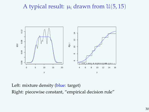
A typical result: µi drawn from U(5, 15)

Koenker and Mizera 9

the monotonicity requirement and perform quite well as we shall see inSection 5.

0 5 10 15 20

0.00

0.04

0.08

0.12

y

g(y)

4 6 8 10 12 14 16

68

1012

14y

δ(y)

Figure 1. Estimated mixture density, g, and correspondingBayes rule, δ, for a simple compound decision problem.The target Bayes rule and its mixture density are plottedas smooth (blue) lines. The local maxima give y for whichδ(y) = y.

4.2. Nonparametric maximum likelihood. Let {u1, ...,um} be a fixed gridas above. Let A be the n by m matrix, with the elements ϕ(Yi − uj) in thei-th row and j-th column. Consider the (primal) problem,

min{−

n∑

i=1

log(gi) | Af = g, f ∈ S},

where S denotes the unit simplex in Rm, i.e. S = {s ∈ Rm|1>s = 1, s > 0}.So fj denotes the estimated mixing density estimate f evaluated at thegrid point uj, and gi denotes the estimated mixture density estimate, g,evaluated at Yi. In this case it is again somewhat more efficient to solve thecorresponding dual problem,

max{

n∑

i=1

log νi | A>ν 6 n1m, ν > 0},

and subsequently recover the primal solutions. For the present purpose ofestimating an effective Bayes rule, a relatively fine fixed grid like that usedfor the EM iterations seems entirely satisfactory.

Left: mixture density (blue: target)Right: piecewise constant, “empirical decision rule”

30

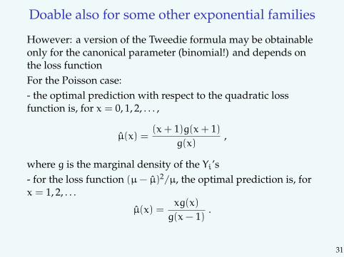
Doable also for some other exponential families

However: a version of the Tweedie formula may be obtainableonly for the canonical parameter (binomial!) and depends onthe loss functionFor the Poisson case:- the optimal prediction with respect to the quadratic lossfunction is, for x = 0, 1, 2, . . . ,

µ(x) =(x+ 1)g(x+ 1)

g(x),

where g is the marginal density of the Yi’s- for the loss function (µ− µ)2/µ, the optimal prediction is, forx = 1, 2, . . .

µ(x) =xg(x)

g(x− 1).

31

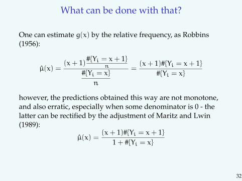
What can be done with that?

One can estimate g(x) by the relative frequency, as Robbins(1956):

µ(x) =(x+ 1)#{Yi = x+ 1}

n

#{Yi = x}n

=(x+ 1)#{Yi = x+ 1}

#{Yi = x}

however, the predictions obtained this way are not monotone,and also erratic, especially when some denominator is 0 - thelatter can be rectified by the adjustment of Maritz and Lwin(1989):

µ(x) =(x+ 1)#{Yi = x+ 1}

1 + #{Yi = x}

32

Better: monotonizations

The suggestion of van Houwelingen & Stijnen (1983): pooladjacent violators - also requires a gridOr one can estimate the marginal density under theshape-restriction that the resulting prediction is monotone:

(x+ 1)g(x+ 1)g(x)

6(x+ 2)g(x+ 2)g(x+ 1)

After reparametrization in terms of logarithms, the problem isalmost linear: linear constraint resulting from the one above,and linear objective function - with a nonlinear Lagrange termensuring that the result is a probability mass function. At anyrate, again a convex problem - and the number of variables isthe number of the x’s

33

Why all this is feasible: interior point methods

(Leave optimization to experts)Andersen, Christiansen, Conn, and Overton (2000)We acknowledge using Mosek, a Danish optimization softwareMosek: E. D. Andersen (2010)PDCO: Saunders (2003)Nesterov and Nemirovskii (1994)Boyd, Grant and Ye: Disciplined Convex Programming

Folk wisdom: “If it is convex, it will fly.”

34

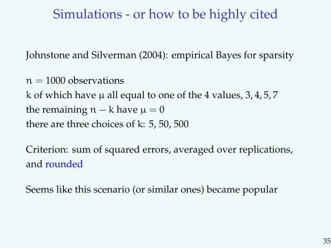
Simulations - or how to be highly cited

Johnstone and Silverman (2004): empirical Bayes for sparsity

n = 1000 observationsk of which have µ all equal to one of the 4 values, 3, 4, 5, 7the remaining n− k have µ = 0there are three choices of k: 5, 50, 500

Criterion: sum of squared errors, averaged over replications,and rounded

Seems like this scenario (or similar ones) became popular

35

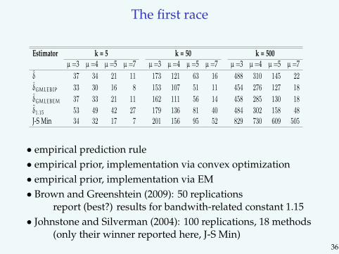
The first raceKoenker and Mizera 7

Estimator k = 5 k = 50 k = 500µ =3 µ =4 µ =5 µ =7 µ =3 µ =4 µ =5 µ =7 µ =3 µ =4 µ =5 µ =7

δ 37 34 21 11 173 121 63 16 488 310 145 22

δGMLEBIP 33 30 16 8 153 107 51 11 454 276 127 18

δGMLEBEM 37 33 21 11 162 111 56 14 458 285 130 18

δ1.15 53 49 42 27 179 136 81 40 484 302 158 48J-S Min 34 32 17 7 201 156 95 52 829 730 609 505

Table 2. Risk of Shape Constrained Rule, δ compared to: two ver-sions of Jaing and Zhang’s GMLEB procedure, one using 100 EMiterations denoted GMLEBEM and the other, GMLEBIP, using theinterior point algorithm described in the text, the kernel procedure,δ1.15 of Brown and Greenshtein, and best procedure of Johnstoneand Silverman. Sum of squared errors in n = 1000 observations.Reported entries are based on 1000, 100, 100, 50 and 100 replica-tions, respectively.

Estimator n = 10,000 n = 100,000k =100 k =300 k =500 k =500 k =1000 k =5000

δGMLEB 268 703 1085 1365 2590 10709

δ 282 736 1136 1405 2659 10930

δ1.05 306 748 1134 2410 3810 10400Oracle 295 866 1430 3335 5576 16994

Table 3. Empirical Risk of a gridded version of the GMLEB rule,the Shape Constrained Rule, δ, compared to kernel procedure, δ1.05

of Brown and Greenshtein, and an oracle hard threshholding ruledescribed in the text. The first two rows of the table are based on1000 replications. The last two rows are as reported in Brown andGreenshtein and based on 50 replications.

taken from Brown and Greenshtein (2009). The row labeled “strong oracle,” alsotaken from Brown and Greenshtein (2009), is a hard-thresholding rule which takesδ(X) to be either 0 or X depending on whether |X| > C for an optimal choice of C.Since the shape constrained estimator is quite quick we have done 1000 replica-tions, while the other reported values are based on 50 replications as reported inBrown and Greenshtein (2009). As in the preceeding table the reported values arethe sum of squared errors over the n observations, averaged over the number ofreplications. Again, the shape constrained estimator performs quite satisfactorily,while circumventing difficult questions of bandwidth selection.

Given the dense form of the constraint matrix A, neither the EM or IP formsof the GMLE methods are feasible for sample sizes like those of the experimentsreported in Table 3. Solving a single problem with n = 10, 000 requires aboutone hour using the Mosek interior point algorithm. However, it is possible to binthe observations on a fairly fine grid and employ a slight variant of the proposedinterior point approach in which the likelihood terms are weighted by the rela-tive (multinomial) bin counts. This approach, when implemented with a equallyspaced grid of 600 points yields the results in the first row of Table 3. Not toounexpectedly given the earlier results, this procedure performs somewhat better

• empirical prediction rule• empirical prior, implementation via convex optimization• empirical prior, implementation via EM• Brown and Greenshtein (2009): 50 replications

report (best?) results for bandwith-related constant 1.15• Johnstone and Silverman (2004): 100 replications, 18 methods

(only their winner reported here, J-S Min)36

A new lineup

2 3 4 5 6 7BL 299 386 424 450 474 493DL(1/n) 307 354 271 205 183 169DL(1/2) 368 679 671 374 214 160HS 268 316 267 213 193 177EBMW 324 439 306 175 130 123EBB 224 243 171 92 53 45EBKM 207 223 152 79 44 37oracle 197 214 144 71 34 27

Bhattacharya, Pati, Pillai, Dunson (2012): “Bayesian shrinkage”BL: “Bayesian Lasso”DL: “Dirichlet-Laplace priors” (with different strengths)

HS: Carvalho, Polson, and Scott (2009) “horseshoe priors”EBMW: “asympt. minimax EB” of Martin and Walker (2013)

elsewhere: Castillo & van der Vaart (2012) “posterior concentration”

37

Comments (Conclusions ?)

• both approaches typically outperform other methods• Kiefer-Wolfowitz empirical prior typically outperformsmonotone empirical Bayes (for the examples we considered!)• both methods adapt to general P, in particular to those withmultiple modes• however, Kiefer-Wolfowitz empirical prior is more flexible:(much) better adapts to certain peculiarities vital in practicaldata analysis, like unequal σi, inclusion of covariates, etc• in particular, it also exhibits certain independence of thechoice of the loss function (the estimate of the prior, and henceposterior is always the same)• but, in certain situations Kiefer-Wolfowitz (on the grid!) maybe more computationally demanding

38

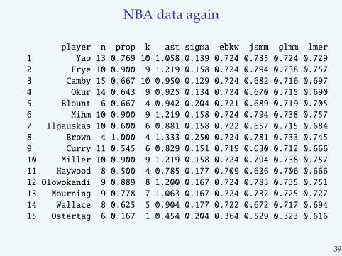
NBA data again

player n prop k ast sigma ebkw jsmm glmm lmer

1 Yao 13 0.769 10 1.058 0.139 0.724 0.735 0.724 0.729

2 Frye 10 0.900 9 1.219 0.158 0.724 0.794 0.738 0.757

3 Camby 15 0.667 10 0.950 0.129 0.724 0.682 0.716 0.697

4 Okur 14 0.643 9 0.925 0.134 0.724 0.670 0.715 0.690

5 Blount 6 0.667 4 0.942 0.204 0.721 0.689 0.719 0.705

6 Mihm 10 0.900 9 1.219 0.158 0.724 0.794 0.738 0.757

7 Ilgauskas 10 0.600 6 0.881 0.158 0.722 0.657 0.715 0.684

8 Brown 4 1.000 4 1.333 0.250 0.724 0.781 0.733 0.745

9 Curry 11 0.545 6 0.829 0.151 0.719 0.630 0.712 0.666

10 Miller 10 0.900 9 1.219 0.158 0.724 0.794 0.738 0.757

11 Haywood 8 0.500 4 0.785 0.177 0.709 0.626 0.706 0.666

12 Olowokandi 9 0.889 8 1.200 0.167 0.724 0.783 0.735 0.751

13 Mourning 9 0.778 7 1.063 0.167 0.724 0.732 0.725 0.727

14 Wallace 8 0.625 5 0.904 0.177 0.722 0.672 0.717 0.694

15 Ostertag 6 0.167 1 0.454 0.204 0.364 0.529 0.323 0.616

39

A (partial) picture

0.2 0.4 0.6 0.8 1.0

0.2

0.4

0.6

0.8

1.0

nba$prop

nba$prop

pkwglmmlmerjs

40

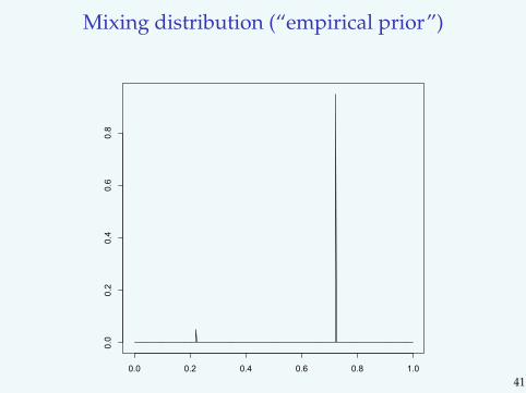
Mixing distribution (“empirical prior”)

0.0 0.2 0.4 0.6 0.8 1.0

0.0

0.2

0.4

0.6

0.8

41

Mixing distribution for glmm

0.0 0.2 0.4 0.6 0.8 1.0

0.0

0.2

0.4

0.6

0.8

pgr

nba.glmm$p

42

The auto insurance predictions

0 1 2 3 4 5 6 7

01

23

45

6

acd$rate

acd.mon$robbmon

43

That’s it?

What if P is unimodal? Cannot we do better in such a case?

And if we can, will it be (significantly) better than James-Stein?

Joint work with Mu Lin

45

OK, so just impose unimodality on P ...

... or more precisely, constrain P to be log-concave (or q-convex)(unimodality does not work well in this context)

However, the resulting problem is not convex!

Nevertheless, given that:log-concavity of P + that of ϕ implies that of the convolution

g(y) =

∫ϕ(y− µ)dP(µ)

one can impose log-concavity on the mixture!(So that the resulting formulation then a convex problem is.)

46

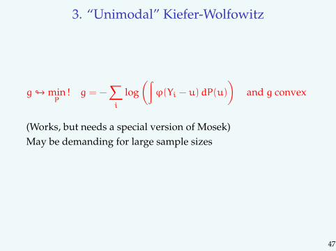
3. “Unimodal” Kiefer-Wolfowitz

g# minP

! g = −∑

i


)

(Works, but needs a special version of Mosek)May be demanding for large sample sizes

47


g# minP

! g = −∑

i


)and g convex


47


g# ming,P

! g > −∑

i


)and g convex


47

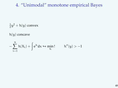
4. “Unimodal” monotone empirical Bayes

12y

2 + h(y) convex

h(y) concave

−

n∑

i=1

h(Xi) +

∫ehdx# min

h!

12y2 + h(y) convex

Very easy, very fast

48


12y

2 + h(y) convex

h(y) concave

−

n∑

i=1

h(Xi) +

∫ehdx# min

h! 1 + h′′(y) > 0


48


12y

2 + h(y) convex

h(y) concave

−

n∑

i=1

h(Xi) +

∫ehdx# min

h! h′′(y) > −1


48


12y

2 + h(y) convex

h(y) concave

−

n∑

i=1

h(Xi) +

∫ehdx# min

h! 0 > h′′(y) > −1


48

A typical result, again from U(5, 15)

5 10 15

0.00

0.02

0.04

0.06

0.08

0.10

0.12

y

Mixture density

5 10 15

68

1012

14y

Prediction rule

(Empirical prior, mixture unimodal)

49

A typical result, again from U(5, 15)

5 10 15

0.00

0.02

0.04

0.06

0.08

0.10

0.12

y

Mixture density

5 10 15

68

1012

14y

Prediction rule

(Empirical prediction rule, mixture unimodal)

50

Some simulations

Sum of squared errors, averaged over replications, rounded

U[5, 15] t3 χ22 095|205 050|250 095|505 050|550

br 101.5 112.4 77.8 19.7 57.3 12.6 21.1kw 92.6 114.4 71.9 17.4 51.3 10.0 17.0brlc 85.6 98.1 67.6 17.3 51.7 21.6 58.2kwlc 84.9 98.2 66.8 16.5 50.4 21.2 67.6mle 100.2 100.1 100.2 100.7 100.4 100.1 99.6js 89.8 98.5 80.2 18.5 52.1 56.2 86.8oracle 81.9 97.5 63.9 12.6 44.9 4.9 11.5

Last four: the mixtures of Johnstone and Silverman (2004):n = 1000 observations, with 5% or 50% of µ equal to 2 or 5and the remaining ones are 0

51

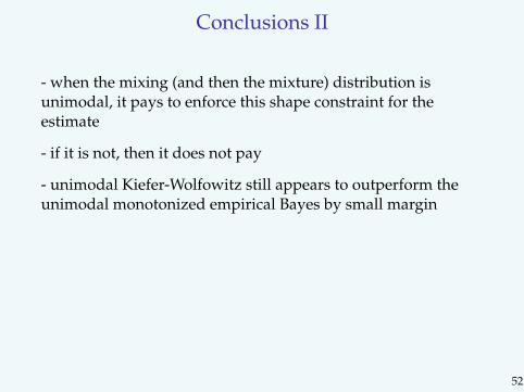
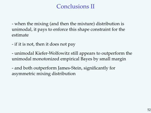
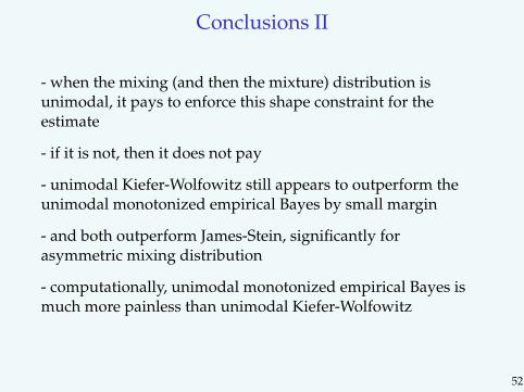
Conclusions II

- when the mixing (and then the mixture) distribution isunimodal, it pays to enforce this shape constraint for theestimate

- if it is not, then it does not pay

- unimodal Kiefer-Wolfowitz still appears to outperform theunimodal monotonized empirical Bayes by small margin

- and both outperform James-Stein, significantly forasymmetric mixing distribution

- computationally, unimodal monotonized empirical Bayes ismuch more painless than unimodal Kiefer-Wolfowitz

52

Borrowing Strength from Experience: Empirical Bayes...

Documents

Transcript of Borrowing Strength from Experience: Empirical Bayes...