Bootstrap Markov chain Monte Carlo and optimal solutions ...

Bootstrap Markov chain Monte Carlo 1

Bootstrap Markov chain Monte Carlo and optimal solutions for the Law of

Categorical Judgment (Corrected)

Greg Kochanski and Burton S. Rosner

University of Oxford

Corresponding author: Burton S Rosner, 2 Ryeford Court, Wish Ward, Rye

TN31 7DH, U. K.; Tel.: (44)1797225714; email: [email protected].

This paper can be obtained from http://kochanski.org/gpk/papers/2009/burt2.pdf , from the Oxford University Library

Service, or from http://arxiv.org/abs/1008.1596 . It should be referenced as: Greg Kochanski and Burton S. Rosner,

“Bootstrap Markov chain Monte Carlo and optimal solution for the Law of Categorical Judgment (Corrected)” (2010)

arXiv:1008.1596v2 http://arxiv.org/abs/1008.1596 .

Running head: Bootstrap Markov chain Monte Carlo

Bootstrap Markov Chain Monte Carlo 2

Abstract

A novel procedure is described for accelerating the convergence of Markov chain

Monte Carlo computations. The algorithm uses an adaptive bootstrap technique to

generate candidate steps in the Markov Chain. It is efficient for symmetric, convex

probability distributions, similar to multivariate Gaussians, and it can be used for

Bayesian estimation or for obtaining maximum likelihood solutions with confidence

limits. As a test case, the Law of Categorical Judgment (Corrected) was fitted with

the algorithm to data sets from simulated rating scale experiments. The correct

parameters were recovered from practical-sized data sets simulated for Full Signal

Detection Theory and its special cases of standard Signal Detection Theory and

Complementary Signal Detection Theory.

Keywords: Markov chain Monte Carlo, rating scale, Law of Categorical Judgment

(Corrected).


The Markov-Chain Monte-Carlo (MCMC) technique originated in statistical

physics (Metropolis, Rosenbluth, Rosenbluth, Teller, & Teller, 1953). It has since

spread into other fields, including psychology (e. g., Béguin & Glas, 2001; Griffiths,

Steyvers, & Tenenbaum, 2007; Morey, Rouder, & Speckman, 2008; Sanborn,

Griffiths, & Shiffrin, 2010). Typically, MCMC is used to compute samples from the

stationary probability distribution π of a Markov chain. In the MCMC algorithm, only

ratios of π (or of likelihoods) need be calculated, so normalization of π becomes

unnecessary. This simplification is a major advantage, since normalization requires a

multidimensional integral over π that is often computationally impractical.

The original MCMC algorithms (e.g., Metropolis et al., 1953; Hastings, 1970)

were simple. From position zt, compute a test position xt = zt +v, where v is drawn

from a distribution V that generates the steps of a random walk. Then accept xt with

probability min[π(xt)/ π (zt); 1], either setting zt+1 = xt or else rejecting xt and setting

zt+1 = zt.

The generator V is relatively unimportant asymptotically, because almost any

reasonable V will make the MCMC chain converge on the same distribution π.

Practically, however, V is critical, especially for high-dimensional problems. Bad

choices of V can dramatically increase the time needed to sample all of π.1 To

1 For instance, assume π is an N-dimensional spherical multivariate normal distribution, with unit variances (i.e. the covariance matrix is the identity matrix I). For a step-generator matrix V that is φI, the probability of accepting a step asymptotically scales as φ-N, for φ>>1, as one would expect from the scaling of a N-dimensional sphere. So, for example, in a 30-dimensional problem, if one starts with V too large by just a factor of two, the step acceptance probability will be near 10-10. A Monte-Carlo sampling algorithm will, in consequence, slow to a crawl. Choosing φ too small is less dramatic but also leads to poor performance. Asymptotically, for φ<<1, the step acceptance rate is high, but it takes on the order of φ-2 steps to move from one side of π to the other. The samples that are generated become strongly correlated and, again, the algorithm slows.


address this problem, procedures have been devised that compute V based on the

history of the chain (e.g., Gelfand & Sahu, 1994; Gilks, Roberts, & Sahu, 1998;

Atchadé & Rosenthal, 2005).

We now describe a novel algorithm, termed bootstrap Markov chain Monte

Carlo (BMCMC) that also uses the chain's history to construct V. In the latter half of

this paper. It will start and operate efficiently even with choices of V that are

substantially different from the optimal values (i.e. with eigenvalues that by several

orders of magnitude). This is valuable from a practical point of view, especially with

new and/or nonlinear problems, because V is often not knowable in advance.

BMCMC is applied to obtain maximum likelihood solutions to a general

equation for rating data, the Law of Categorical Judgment (Corrected) (Rosner &

Kochanski, 2009). Our procedures go well beyond the earlier treatment of rating data

by Schönemann and Tucker (1967).

Bootstrap Markov Chain Monte Carlo

Bootstrap Markov chain Monte Carlo rests on standard Markov chain Monte

Carlo procedures (Anonymous, 1998; Geyer,1992; Gilks, Richardson, &

Spiegelhalter, 1995). Like any MCMC algorithm, it takes iterative steps, constantly

updating a vector of parameters p�

. The algorithm, however, adapts itself to the

probability distribution. It adjusts its steps to achieve efficient sampling of probability

densities that are approximately multivariate-Gaussian; but it proceeds in such a way

that violations of the Markov assumptions become asymptotically negligible. It can


produce chains of samples that converge rapidly to π for approximately symmetric

and convex densities.

The algorithm is robust. It can handle functions that are not computable (in

the practical sense) at certain points; and it does not assume that π is smooth or

continuous, so long as it is bounded above. Finally, BMCMC can be used on

functions that stochastically approximate π, where the computable approximation to π

is a random variable, and successive computations of π with the same parameters may

give different values.2 Experience has shown that this makes it workable for many

types of computation where common procedures are unsuitable. One example is

computation of π by sampling techniques such as a Monte-Carlo integral. Another

example is where π is a noisy measurement of some physical property.

The BMCMC procedure can be run in either of two closely related modes:

optimisation or sampling. In optimisation mode, it searches for parameter values that

best explain the data under analysis, by maximizing log likelihood log(L), perhaps

modified by a Bayesian prior.3 In sampling mode, BMCMC repeatedly samples from

π, which is proportional to the log(L) or to a Bayesian posterior density. This allows

calculation of all necessary statistics, including confidence limits for the optimal

parameters and for the observations predicted from those parameters.

The following description of BMCMC is somewhat simplified. The source

code should be consulted for details; footnotes give references into the code. The

2 This has yielded good behaviour in certain test cases, but no proofs are available. To do this, use mcmc.position_nonrepeatable instead of the default mcmc.position_repeatable .


algorithm is embodied in two main python modules, mcmc.py and mcmc_helper.py.

They are in release gmisclib-0.65.5 which, along with all other code described here,

can be downloaded from http://sourceforge.net/projects/speechresearch or under

http://phon.ox.ac.uk.

Braun, Kochanski, Grabe, and Rosner (2006) and Alvey, Orphanidou,

Coleman, McIntyre, Golding, and Kochanski (2008) used earlier versions of this code

(albeit with minimal description). In other work, we have successfully tested

BMCMC on moderately high-dimensional problems. We also have shown

convergence to expected solutions and reasonable error bars for 200-dimensional

problems.

Application of BMCMC requires a user-supplied software module that

produces the log of a value proportional to π. In optimisation mode, for example,

π( p�

)would be the probability with which a model with parameters p�

would generate

the observed data. The problem-specific module takes a vector of tentative

parameters p�

from the BMCMC process. The module first may modify p�

to account

for symmetries or constraints on the distribution.4 Then it computes the log likelihood

log(L) for the resulting parameters,5 finally returning log(L) to the BMCMC

algorithm.

Optimisation Mode

3 We focus here to the widely used log(L), but this mode can also be used for Bayesian model fitting. In practical terms, the Bayesian posterior probability is just the likelihood, multiplied by the prior probability, then normalized to have a unit integral. 4 In the code, this can be done by implementing mcmc.problem_definition.fixer . 5 By means of mcmc.problem_definition.logP .


The central operation of the BMCMC algorithm increments the current

parameter vector p�

by a quasi-random step vector d�

. The difference

D= log(L( p�

+d�

))-log(L( p�

)) is computed. If log(L) improves (D>0), the new

location is accepted. If log(L( p�

+ d�

)) cannot be computed, the step is rejected,

leaving the procedure at its prior location. If D is negative, the new location is

accepted with the Metropolis probability e-D (or e-D/T when using the algorithm for

simulated annealing at temperature T). Then the process iterates from its current

location. As the algorithm progresses, log(L) generally increases, and an optimal

solution for the parameters finally emerges.

Step determination. Bootstrap Markov chain Monte Carlo uses two schemes

for generating d�

. After an initial start-up period, an adaptive bootstrap resampling

procedure is used to generate 90 per cent of the steps.6 Otherwise, the step comes

from a pre-specified multivariate Gaussian density (with adaptive, diagonal scaling).7

The bootstrap procedure randomly chooses two vectors from an archive of

previously accepted parameter vectors. The difference between them becomes the

current step. In principle, bootstrapping violates the Markov assumption that each

6 4See the BootStepper class in mcmc.py. The 90% fraction was chosen somewhat arbitrarily as a

compromise between accelerating the algorithm in good conditions and robustness under difficult

conditions. This causes a 10% performance loss under good conditions in exchange for a guarantee

that the performance will not be more than 10 times worse than an adaptive (but non-bootstrap)

algorithm if the distribution were very different from multivariate normal.

7 See the StepV method in the BootStepper class in mcmc.py.


step is independent of its predecessors, because the archive contains the history of the

algorithm’s computations. However, as the archive lengthens, the density of samples

from it asymptotically approaches π and becomes stationary. Therefore, when the

archive holds a sufficiently large number of samples widely distributed across π, the

Markov assumption will be satisfied to any required accuracy. We later show that the

archive size becomes asymptotically infinite, making the system approach a Markov

chain.

The bootstrapping scheme works well when the density of log(L) is close to a

multivariate Gaussian, even a highly elongated one. This is because a large enough

archive makes the step probability density approach the convolution

( ) ( ) ( )P d p p d dpπ π= ∗ +∫� �

� � �

. If ( )pπ � is a multivariate Gaussian, then ( )P d�

will also

be. It will have the same shape and orientation as ( )pπ � but twice the variance. As a

result, the long axes of the distribution will be accurately aligned with those of π.

The BMCMC algorithm tracks the proportion fλ of bootstrap steps accepted

over a period tλ. This proportion controls a factor λ that multiplies d�

. When fλ

significantly8 exceeds1/4, λ is increased, thus decreasing the acceptance rate. When

the proportion falls significantly below 1/4, λ is decreased with the opposite effect.

If ( )pπ � is multivariate Gaussian, λ converges to its final value within a few hundred

steps. Its final value depends on the number of dimensions and on the details of

( )pπ � but is typically slightly smaller than unity.


This procedure for controlling λ can sometimes behave badly if ( )pπ � drops

rapidly, especially discontinuously, to zero, e.g. in an optimization problem where

p�

is subject to hard-wall constraints. If three or more hard walls meet, they can form

a corner where locally even small steps are less than 25 per cent likely to be accepted.

This lowers the average step acceptance rate, and the algorithm responds by reducing

λ, which in turn slows computation. If hard-wall constraints are desired, see the

Appendix.

In principle, adjusting fλ also violates the Markov assumption, because the

scaling depends on recent history. The period tλ, however, increases during

optimisation. Eventually, tλ becomes longer than the time required for BMCMC to

explore all of π. The dependence of λ on history then becomes unimportant, and the

algorithm asymptotically produces a Markov chain. We insure that this happens by

making the required significance level for deciding when to change fλ an increasingly

stringent function of the number of iterations since the most recent reset.9 Resets are

described below.

The pre-specified step generator draws from a multivariate Gaussian density

V* for the first few steps. Then a scaled version of V* is used to generate 10 per cent

of the later steps. The scale factor similarly depends on the fraction of recently

accepted steps and is proportional to the square root of the parameter-by-parameter

8 See mcmc.adjuster._inctry_guts and mcmc.BootStepper.step_boot for details. The required significance level starts low and is gradually raised, so that symptotically, the probability of falsely adjusting λ goes to zero, and the interval between adjustments becomes infinite. 9 See _inctry_guts in the adjuster class in mcmc.py.


standard deviation of the archive.10 Again, as tλ and the archive lengthen, this step

generator also asymptotically behaves as a Markov chain.

The two methods of step selection compensate for each other's deficiencies.

Alone, the pre-specified step distribution can cause slow convergence and slow

exploration of ( )pπ � if the shape or orientation of V* does not match that of π.

Nevertheless, this method will eventually explore all of ( )pπ � .

The bootstrap method needs the pre-specified distribution procedure to

initialise the archive. Furthermore, bootstrapping is limited to linear combinations of

archive points. Hence, if all archived vectors fell in a low dimensional subspace ϖ of

( )pπ � , bootstrapping would remain there. Mixing the two methods of step selection

avoids that trap, because picking from the pre-specified distribution will soon

engineer an escape from ϖ .

Operation. Optimisation mode is broadly similar to simulated annealing

(Press, Teukolsky, Vettering, & Flannery, 2002, pp. 448-458), including a system

temperature.11 Early on, large decreases in π are allowed, corresponding to a high

system temperature. The default annealing schedule decreases the temperature

whenever a step is accepted, eventually approaching a specified target temperature.12

(The annealing schedule can be redesigned by changing parameters or re-

implementing the mcmc_helper.step_acceptor object.) The algorithm stores the

10 The algorithm is reasonably robust to a mismatch between V and π. In practice, it frequently tolerates a two orders of magnitude mismatch in standard deviation, especially in optimization mode. Starting in sampling mode can be slow if the initial step acceptance probability is low. 11 The high level interface to optimization mode is mcmc_helper.stepper.run_to_bottom .


maximum value of log(L) encountered so far. If a new value appears that exceeds the

old one by half the temperature, the algorithm is partially reset: the temperature is

raised slightly, all counters are reset, tλ is decreased, and the archive is shortened by

eliminating those p�

that give the smallest log(L).13 Additionally, over the next 2Np

accepted steps, each step begins at the parameters that give the maximal log(L) rather

than the most recent parameter vector.14 (Here, Np is the number of unconstrained

parameters.) This can substantially improve the rate at which the algorithm first

approaches a minimum. The search then continues.

Resets serve several purposes. Raising the temperature can help the algorithm

to escape a local maximum. Shortening the archive and tλ facilitates adaptation of the

search to the shape of log(L).

For any π with an upper bound, the tolerance of 0.5T for log(L) guarantees

that there will be only a finite number of resets. Consequently, there will be a final

reset, after which both the archive size and the tracking period tλ will approach

infinity. This is necessary for BMCMC to become asymptotically Markovian.

Optimisation termination. The BMCMC optimisation mode terminates15

when two conditions are met.16 First, successive accepted values of p�

must show no

12 The annealing schedule can be redesigned by changing parameters or re-implementing the step_acceptor object in mcmc_helper.py. 13 See mcmc.BootStepper.reset . 14 See code that uses mcmc.Archive.sorted . 15 Note that these termination criteria are strictly heuristics: nothing is provable except that optimization mode will eventually terminate. 16 Optimization mode is the run_to_bottom method in the stepper class in mcmc_helper.py. See the _not_at_bottom method of the stepper class in mcmc_helper.py.


systematic drift. Second, enough steps must have occurred to match an estimate of

the number needed to explore all of π.

Drift is evaluated by sampling archived p�

every Na accepted steps (Na is set

at 24 in the examples below). Difference vectors are computed between adjacent

samples, and the angles between pairs of successive difference vectors are found. If

p�

systematically drifts, the difference vectors will point in a common direction.

Otherwise, reversals in direction will occur, and the angles will frequently exceed π/2

radians. The algorithm counts the number of such reversals since the last reset.17 The

termination condition of no systematic drift is met when the count reaches a suitable

threshold.

The second termination condition requires an estimate of the number of steps

needed to explore all of π. The algorithm uses a bent multivariate Gaussian model to

make this estimate. The density of log(L) is represented as approximately multivariate

Gaussian, but the longest axis of the probability ellipsoid is assumed to be slightly

curved. This curvature limits the length of steps along the bent direction. Since steps

are straight, long steps would fall off the likelihood ridge, yielding small values of

log(L) that typically would be rejected. These small steps then form a random walk

along the longest axis.

The curvature in the model is related to the factor λ that scales the bootstrap

step size. It should take on the order of 2λ − accepted steps for a random walk to

17 Direction changes are accumulated in the dotchanged and xchanged variables in stepper.run_to_bottom in mcmc_helper.py.


explore the length of the density.1815 Accordingly, the second termination condition is

that the number of steps accepted since the last reset exceeds a constant times2λ − .19

(N.B.: if there are k≥2 comparably large eigenvalues of the covariance matrix, this

termination condition may fire early.)

Sampling Mode

After optimisation finishes, the BMCMC procedure can be run in sampling

mode, producing various confidence intervals.20 The algorithm randomly samples a

probability density ( )pπ � , proportional to log ( )L p�

, in the vicinity of the solution.

The system temperature is held at unity, and steps are accepted in accordance with

the Metropolis algorithm.21 Each sample of p�

is archived.

Sampling mode sometimes finds a new maximum of log(L). If so, the

previously described reset procedures apply, except that now the oldest archived

samples are dropped and the temperature remains fixed at unity. In sampling mode,

the archive becomes very long after the final reset. If it needs shortening, e.g., to limit

computer memory consumption, the oldest samples would be dropped. Given

sufficient time and memory, sampling from the archive becomes a good

approximation of sampling from ( )pπ � .

18 Computed in Bootstepper.ergodic in mcmc.py. 19 This information is accumulated in the “es” variable in stepper.run_to_bottom in mcmc_helper.py. N.B.: if there are k≥2 comparably large eigenvalues of the covariance matrix, this termination condition may fire early; it assumes that there is a single long axis to π. 20 The high-level interface to sampling mode is mcmc_helper.stepper.run_to_ergodic . 21 We emphasize that in sampling mode, as long as the probability density is bounded above, the BMCMC algorithm will always, asymptotically approach a Metropolis algorithm, and all the properties of that will then apply. So, BMCMC will not misbehave in the sense of giving wrong answers, though (as with all MCMC algorithms) it is difficult to know when one has collected enough samples.


Sampling termination. The BMCMC algorithm stops when the desired

number of samples, Ne, from ( )pπ � have been stored and enough steps have been

accepted to explore the longest axis of the density approximately Ne times.22

Iterations continue as long as 21/ 1.4i p ei

N Nλ <∑ , where λi is the step scaling factor λ

at the ith iteration and Np is the number of free parameters. This proviso flows from

the same bent random walk model that imposes a termination condition on

optimisation mode. Within the limits of that model, the inequality insures getting

least Ne independent samples from ( )pπ � . The summation starts anew whenever the

algorithm resets itself, so iterations cannot terminate while log(L) continues to

improve.

Confidence intervals. The archive resulting from repeated sampling yields

confidence limits for the parameters and for the predicted data. All the usual

statistics, such as the means and variance of parameters, are integrals over( )pπ � . Any

such integral can be approximated by a sum over samples from ( )pπ � . Confidence

intervals can be computed from estimates of means and variances or determined

directly from cumulants of the samples.

Optimal Solutions for the Law of Categorical Judgment (Corrected)

We now illustrate the use of BMCMC for multidimensional nonlinear

optimisations, including computation of error bars. The Law of Categorical Judgment

(Torgerson, 1958; McNicol, 1972) is a general model for any rating experiment. On

each trial t, one stimulus Sh is randomly selected for presentation from a pool of N

22 See the “nc” variable in stepper.run_to_ergodic in mcmc.py.


stimuli. The subject responds with one of M+1 possible ordered responses Ri.

According to the law, each stimulus projects an independent random Gaussian

density S Sφ(x;µ ,σ )h h

of possible impressions on a one-dimensional psychological

continuum v. On trial t, the observer draws one sample with value st on v from the

signal density for Sh. Only the experimenter knows which Sh actually produced st. On

each trial, the observer also places M criteria at different loci on ν. The criteria divide

v into M+1 successive intervals that define the possible responses.

The Law of Categorical Judgment proposes that each criterion also is an

independent random Gaussian variable, C Cφ(x;µ ,σ )i i

, on ν. On trial t, therefore,

criterion positions cit, i = 1, …, M, are drawn from the criterion densities, where i

indexes the order of the density means. The indices are private to the observer. The

observer calculates the M differences st-cit. If st-cjt is the smallest positive difference,

response Rj is selected. The response RM+1 ensues when all differences are negative.

The Law of Categorical Judgment (Corrected)

The long-accepted general equation for the Law of Categorical Judgment

(Torgerson, 1958; McNicol, 1972) is fatally flawed (Rosner & Kochanski, 2009). It

ignores the fact that criterion densities are independent Gaussians. When the densities

overlap sufficiently, criterion samples can get out of order, and the original formula

can yield negative probabilities. Rosner and Kochanski derived a new equation, the

Law of Categorical Judgment (Corrected), that fixes the flaw:


C C S S C C(R |S ) φ( ;µ ,σ ) φ( ;µ ,σ ) [1 φ( ;µ ,σ ) ] . (1)i i

i i h h j j

Mc c

h i j j isj i

P i c s c dc dsdc∞

−∞ −∞≠

= = −∏∫ ∫ ∫

Equation 1 assumes that criteria are independent Gaussian variables.

Nevertheless, it still may apply when response dependencies undercut the

assumption. Criterion-setting theory (Treisman & Williams, 1984) explains how such

dependencies arise in detection and discrimination. Treisman (1985) extended the

theory to absolute judgments, a form of rating. Simulations showed that the resulting

criterion densities were indistinguishable from Gaussians. In effect, response

dependencies would drive the product term in Equation 1 towards unity. The product

term, however, would not necessarily reach unity. When Treisman and Faulkner

(1985) analysed rating data with criterion-setting theory, they found evidence that

criteria interchanged positions. Equation 1 therefore could apply to rating data when

response dependencies occurred.

Two special cases. The familiar signal detection theory (SDT) model for

rating experiments makes criterion positions cit invariant across trials (see Macmillan

& Creelman, 2003, ch. 3). Each criterion density thereby becomes a Dirac delta

function δ(x-ci) (Bracewell, 1999, chap. 5), and the outer integral and product in

Equation 1 simplify away. The result (Rosner and Kochanski, 2009) is

1

S S(R= |S) φ( ;µ ,σ ) .i

i

c

cP i s ds

−

= ∫ (2)

This is equivalent to the standard form for the SDT rating model:


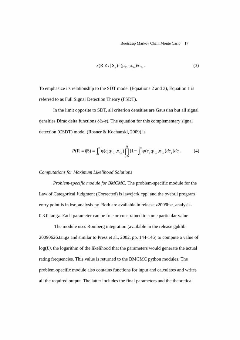
C S S(R | S )=(µ -µ )/σi h hhz i≤ . (3)

To emphasize its relationship to the SDT model (Equations 2 and 3), Equation 1 is

referred to as Full Signal Detection Theory (FSDT).

In the limit opposite to SDT, all criterion densities are Gaussian but all signal

densities Dirac delta functions δ(x-s). The equation for this complementary signal

detection (CSDT) model (Rosner & Kochanski, 2009) is

C C C C(R |S) φ( ;µ ,σ ) [1 φ( ;µ ,σ ) ] .i

i i j j

M c

i j j is sj i

P i c c dc dc∞

≠

= = −∏∫ ∫ (4)

Computations for Maximum Likelihood Solutions

Problem-specific module for BMCMC. The problem-specific module for the

Law of Categorical Judgment (Corrected) is lawcjcrk.cpp, and the overall program

entry point is in bsr_analysis.py. Both are available in release z2009bsr_analysis-

0.3.0.tar.gz. Each parameter can be free or constrained to some particular value.

The module uses Romberg integration (available in the release gpklib-

20090626.tar.gz and similar to Press et al., 2002, pp. 144-146) to compute a value of

log(L), the logarithm of the likelihood that the parameters would generate the actual

rating frequencies. This value is returned to the BMCMC python modules. The

problem-specific module also contains functions for input and calculates and writes

all the required output. The latter includes the final parameters and the theoretical


probabilities ( | )hP R i S= , their respective confidence limits, and values for measures

of goodness of fit described below.

Markov chain Monte Carlo is normally cast in Bayesian terms. Therefore, one

must (formally) consider prior distributions. For this particular application, however,

any reasonable prior will be much broader than the Bayesian posterior distribution,

( )pπ � . Hence, the difference between the Bayesian and the likelihood approaches

becomes moot. One can readily interpret L( p�

) as proportional to the (Bayesian)

conditional probability of observing specified rating frequencies, given

parametersp�

. Samples from ( )pπ � will then reflect the distribution of parameters that

are statistically consistent with the ratings.

Parameter constraints and adjustments. Before calculating log(L), the

problem-specific module imposes four constraints that harmlessly remove

degeneracies in the solutions. First, the mean of the signal density for S1 is fixed at

zero; all other signal means are made positive and are sorted into ascending order.

Second, ascending order is imposed on criterion means (though they may be

negative). Third, any negative signal or criterion standard deviation is made positive.

Fourth, the average of all unconstrained signal and criterion standard deviations is

divided into each unconstrained mean or standard deviation. The average standard

deviation is thereby held at unity, keeping standard deviations in a convenient range.

This rescaling is analogous to the conventional procedure of constraining a signal

density standard deviation to unity. The constraints do not affect any results; they

merely collapse together observationally equivalent solutions; and they make


interpretation of the results easier. (These four are implemented via

mcmc.problem_definition.fixer in mcmc.py; see the Appendix.)

A final adjustment effectively adds a Bayesian prior to log(L) to keep each

standard deviation σ away from zero. Gaussian densities take the form exp(-…/σ2). If

σ becomes small, say around 0.001, the integrands in Equation 1 change rapidly. In

turn, the Romberg routine forces the integration steps to be smaller than σ. A severe

slowing of computation ensues. The program may even terminate prematurely if σ

becomes so small that round-off errors prevent quadrature from achieving the desired

accuracy. To avoid these difficulties, we add 0.1/ uu

σ∑ to log(L), where uσ is any

unconstrained standard deviation. When alluσ exceed 0.1, as generally happens here,

this term hardly affects the solution.

Constraints and adjustments in optimisation mode must be employed

carefully, however strong may be their pragmatic rationale. They can cause incorrect

results if they have noticeable effects at or near a maximum likelihood solution.

Badly formulated constraints also can artificially limit the size of the confidence

intervals obtained in sampling mode. Nonetheless, adding smooth constraints is often

much more efficient computationally than a hard-wall constraint (e.g. setting

log(L( p�

))=-∞ outside the allowed region for log(L( p�

))).

Goodness of fit. In line with Schunn and Wallach (2005), we use four different

ways of comparing the input rating frequencies against the frequencies predicted

from the recovered maximum likelihood parameters. To begin with, we divide each


input frequency by Tr/Sh expresses it as a proportion ( | )hp R i S= of responses i to

stimulus h. Then, the theoretical conditional probabilities ( | )hP R i S= are computed

via Equations 1, 3, or 4 from the optimal parameters. The four procedures for

evaluating goodness of fit require calculation of (a) root-mean-square deviation

(RMSD) between ( | )hp R i S= and ( | )hP R i S= , (b) Pearson’s r2 for the regression of

( | )hp R i S= on ( | )hP R i S= , (c) the regression coefficients b0 and b1 and their 95 per

cent confidence limits and (d) Kullback-Leibler divergence, the relative entropy of

two probability densities p and q (Kullback & Leibler, 1951; Weisstein, n.d.),

specified here as 2(R | S ) log [ (R | S ) / (R | S )]h h hh i

P i P i p i= = =∑∑ .

Tests of The BMCMC Procedure

We used BMCMC to fit the FSDT, SDT, and CSDT models (Equations 1, 3,

and 4, respectively) to pseudo data matrices generated from known parameter values.

The parameters are the means and standard deviations of the densities in a FSDT,

SDT, or CSDT model. One parameter set was chosen independently for each type of

model. Signal and/or criterion standard deviations (as appropriate) were varied

irregularly, as were distances between signal and criterion means.

Pseudo data matrices were generated by trial-by-trial simulation of a rating

experiment with six stimuli and 10 responses (i.e. 9 criteria). On each trial, a sample

was drawn randomly from a signal density along with one sample from each of the 9

criterion densities. Using the decision rule, a response was selected. From each

parameter set, we produced three pseudo data matrices, with 200, 500, and 1000 trials


per stimulus (Tr/Sh), respectively.

Using the appropriate model equation, maximum likelihood parameters were

computed for each pseudo data matrix through the BMCMC algorithm. Ninety-five

per cent confidence limits for the recovered parameters and the theoretical

probabilities ( | )hP R i S= were based on more than 4000 sets of parameters produced

by BMCMC in sampling mode. Three separate fits were made to each pseudo data

matrix, starting from different initial guesses at the parameters. The fit with the

highest log likelihood (excluding the soft constraint 0.1/ uu

σ∑ ) was accepted.

Altogether, we undertook 27 fits (3 models × 3 matrices × 3 starting points).

We assessed the consistency among the three fits to a given matrix. The

absolute difference | log(Lmax) – log(Lmin) | was found between the highest and the

lowest of the three log(L) values. We divided this difference by the degrees of

freedom in the pseudo data matrix. The result for fits of the FSDT, SDT, and CSDT

models was always less than 0.05, indicating good consistency between the three fits

to each pseudo data matrix. All optimisations on a given matrix apparently gave good

approximations to the true maximum likelihood solution.

To compare the generating parameters against those recovered by an

optimisation, any difference in scaling units had to be eliminated. We obtained a

least-squares solution for b in the equation R = bG, where R and G are the recovered

and generating parameters, respectively. Then the recovered parameters R and their

confidence limits were plotted against the rescaled generating parameters GT=bG. For

a successful recovery, the points should fall on or near the major diagonal, and 95 per


cent of the confidence limits should intersect that line.

Recovery results. Figure 1 shows the best set of recovered parameters plotted

against the rescaled generating values for the FSDT-generated pseudo data matrices.

The upper, middle, and lower panels are plots for the matrices with 200 Tr/Sh

(FSDT200), 500 Tr/Sh (FSDT500), and 1000 Tr/Sh (FSDT1000), respectively. Ninety-

five per cent confidence limits appear around each recovered parameter value.

__________________

Figure 1 about here

__________________

The left side of each panel displays four items: the rescaling equation for the

generating parameters; log(LG), the log likelihood produced by evaluating the match

of the pseudo data to the generating parameters; log(LR), the log likelihood for the

recovered parameters; and the number of samples Ne on which the confidence limits

are based. The legend in Figure 1A applies to each panel.

The BMCMC algorithm always found a solution whose log(LR) exceeded the

original log(LG). However surprising this may be at first, it should be expected. The

pseudo data proportions generated by simulation differ randomly from the underlying

probabilities yielded by the generating parameters. Consequently, parameters will

typically occur that fit better than the generating parameters, and a successful

optimisation should find them. Nonetheless, 95 per cent of the rescaled generating


parameters should fall within the confidence limits for the recovered parameters.


The points in each panel of Figure 1 follow the major diagonal well.

Naturally, confidence intervals shrink as Tr/Sh increases. All confidence limits in the

figure intersect the major diagonal. In short, the fits and error bars are perfectly

satisfactory.

Figures 2 and 3 show the results for the SDT and CSDT fits, respectively.

They are organized like Figure 1. Recovered log(LR) was again higher than

generating log(LG). In each of Figures 2C, 3B, and 3C, confidence limits fail once to

intersect the major diagonal. This is predictable: 5 per cent of the total 63 parameters

should yield misses over the long run. The fits to the SDT and CSDT pseudo data

matrices also are excellent.

______________________

Figures 2 and 3 about here

______________________

Goodness of fit. Table 1 presents information on goodness of fit for the results

in Figures 1 through 3. The first three rows refer to the fits of the FSDT model to the

FSDT-generated pseudo data matrices. For these fits, root mean square deviation

(RMSD) was 0.014 at most. The linear regression of p(R=i|Sh) on P(R=i|Sh) yielded

an r2 of at least .95. The 95 per cent confidence limits for the regression coefficients

b1 and b0 included the ideal values of unity and zero, respectively. Finally, the

Kullback-Leibler divergence always fell well below 0.1.


All indicators of goodness of fit tended to improve as Tr/Sh increased. The

high r2 for the 200 Tr/Sh matrix actually left little room for such increases. The

Kullback-Leibler values declined as Tr/Sh increased, because the divergence acts as

an error measure on differences between pseudo-data proportions and theoretical

probabilities. These differences include statistical fluctuations that are larger for

smaller experiments. In short, all calculations indicate good fits of the recovered

theoretical probabilities to the pseudo data proportions.

The results in Table 1 for the CSDT and SDT intra-model fits repeat those for

the FSDT fits. The RMSD values varied between .005 and .012. Again, r2 exceeded

.95. The confidence limits for b1 and b0 always included unity and zero, respectively.

Finally, Kullback-Leibler divergence values were small and decreased from about

0.06 for Tr/Sh=200 to about 0.01 for Tr/Sh=1000.

____________________

Table 1 about here

____________________

Cross-Model Fits

The widespread use of signal detection theory motivates an obvious question.

For practical-size experiments, could SDT still fit data generated by the more

complex FSDT model? To obtain an initial answer, we fitted the SDT model

(Equation 3) to the pseudo data generated by the FSDT model (Equation 1) and


compared the results to those from the previous FSDT intra-model fits. We extended

this cross-model procedure by fitting the CSDT model to the FSDT-generated pseudo

data and fitting the SDT model to the CSDT-generated pseudo data. Again, three

different starting points were used for each fit. This gave nine SDT-to-FSDT fits (3

matrices × 3 starting points), nine CSDT-to-FSDT fits, and nine SDT-to-CSDT fits.

As before, the fits from the three different starting points proved consistent. For each

cross-model fit, however, log(LR) was always somewhat lower than for the

corresponding intra-model fit.

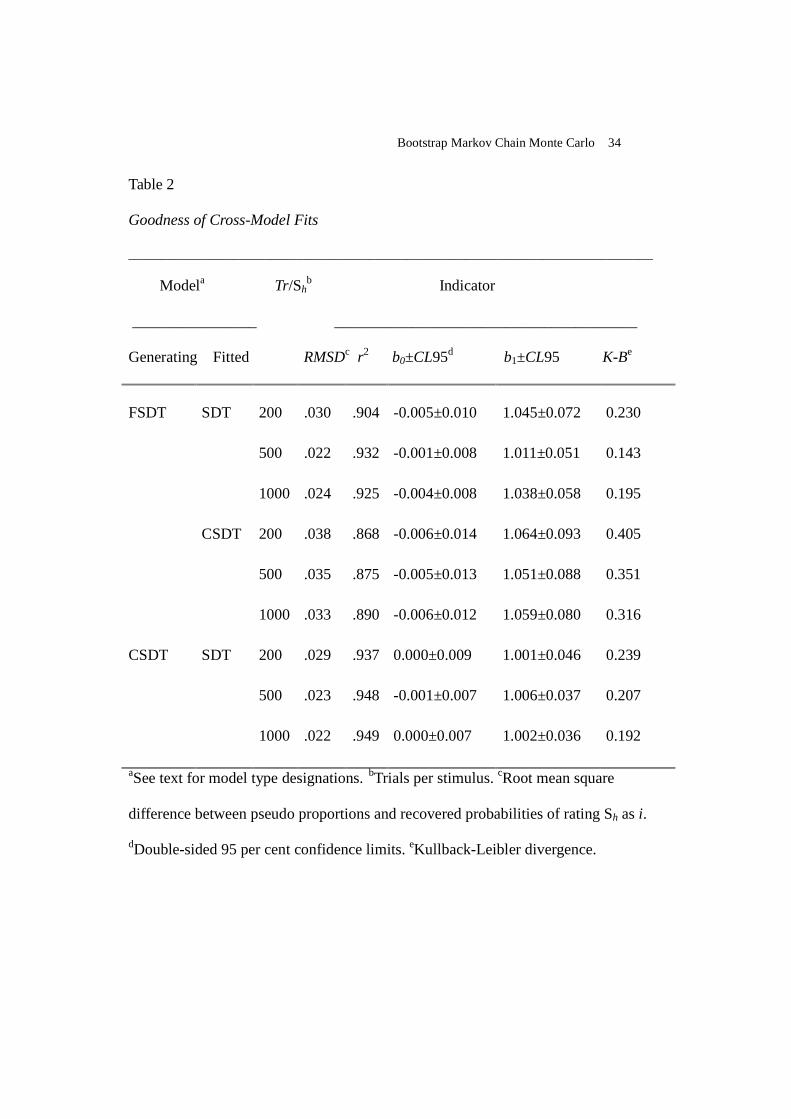
Goodness of fit. Table 2 contains the indicators of goodness of cross-model

fits. Here, RMSD always exceeded 0.02, twice the typical values for intra-model fits.

Furthermore, r2 was .949 at best, even falling to .878. The confidence limits for the

regression coefficients b0 and b1 always exceeded those from the FSDT and CSDT

intra-model fits. Those limits, however, still included the theoretically desirable

values of zero and unity for b0 and b1, respectively. Most noticeably, Kullback-Leibler

divergence always exceeded 0.1, with a median of 0.23. This is above the typical

value for the intra-model fits with Tr/Sh=200 and is about 20 times larger than the

values for intra-model fits with Tr/Sh=1000.

______________________

Table 2 about here

_______________________


The cross-model results indicate that a subject who obeys the FSDT rating

model may produce data beyond the reach of the classical SDT model. Indeed, that

model cannot entirely explain the findings of one study on hearing. Pastore and

Macmillan (2002) undertook an SDT reanalysis of eight sets of rating data originally

collected by Schouten and van Hessen (1998) for an intensity and for a speech

continuum. Except for one data set for intensity, Pastore and Macmillan found that

the SDT model fitted only some ROC curves. Luce’s (1963) low threshold model

seemed to account for the numerous exceptions. This left behind a situation where

two different models had to be invoked to explain single data sets. The FSDT model

may provide an alternative to this unsatisfactory outcome.

CONCLUSIONS

In situations requiring numerical optimisation, the Bootstrap Markov Chain

Monte Carlo algorithm can efficiently provide maximum likelihood solutions and

confidence limits for the parameters. Tests of the algorithm gave good fits of each

variant of the Law of Categorical Judgment (Corrected) to pseudo data matrices

generated by that same variant. Furthermore, measures of goodness of fit showed that

these intra-model fits were better than fits of inappropriate models to the pseudo data.

The way is now open to complete analyses of experimental rating data with the

Gaussian based Law of Categorical Judgment (Corrected).


Appendix

Hard-Wall Constraints and Symmetries

Multiple hard-wall constraints can slow the BMCMC algorithm. However,

hard-wall constraints can often be eliminated by transforming the problem into a

symmetrised version. For instance, consider a truncated normal density

π(y)={ n(y; µ, σ) if y>0; else 0 }. With a hard wall at y=0, samples can be obtained

from a symmetrised variant of π, ζ (q) ∝ n(|q|; µ, σ), and then mapping y = |q|. (Note

that ζ (q) is bimodal if µ >0.) This can be implemented by setting up the “fixer”

method in a class derived from problem_definition so that it maps negative y into

positive y at each step:

class problem_definition(object):

def fixer(self, y):

return numpy.absolute(y)

This kind of substitution can dramatically improve speed, especially if there are

multiple constraints. However, two conditions must be met. First, the mapping needs

to be (at least locally) a reflection around a plane. Second, this technique is known to

work only if the mapping y=M(q) is such that π(M(q)) = ζ (q) for all q, and M is

piecewise isometric linear.

In practice, this works out conveniently if the constraints are orthogonal or

parallel hyperplanes. For instance, if we have a vector p�

= (x, y), the constraints

0<x<1 and y>0 are easy to implement.


References

Alvey, C., Orphanidou, C., Coleman, J., McIntyre, A. Golding, S., &

Kochanski, G. (2008). Image quality in non-gated versus gated reconstruction

of tongue motion using magnetic resonance imaging: a comparison using

automated image processing. International Journal of Computer Assisted

Radiology and Surgery, 3, 457-464.

Anonymous. (1998). Markov chain Monte Carlo in practice: A roundtable

discussion. The American Statistician, 52, 93-100.

Atchadé, Y. F., & Rosenthal, J. S. (2005). On adaptive Markov chain Monte Carlo

algorithms. Bernoulli, 11, 815-828.

Béguin, A. A., & Glas, C. A. W. (2001). MCMC estimation and some model-fit

analysis of multidimensional IRT models. Psychometrika, 66, 541-561.

Bracewell, R. (1999). The Fourier transform and its applications. (3rd ed.) New

York: McGraw-Hill.

Braun, B., Kochanski, G., Grabe, E., & Rosner, B. S. (2006). Evidence for

attractors in English intonation. Journal of the Acoustical Society of America, 119,

4006-4015.

Gelfand, A.E., & Sahu, S. K. (1994). On Markov chain Monte Carlo acceleration.

Journal of Computational and Graphical Statistics, 3, 261-276.

Geyer, C. J. (1992). Practical Markov chain Monte Carlo. Statistical Science, 7,

473-483.

Gilks, W. R., Richardson, S., & Spiegelhalter, D. J. (1995). Markov chain Monte


Carlo in practice. London: Chapman & Hall.

Gilks, W. R., Roberts, G. O., & Sahu, S. K. (1998). Adaptive Markov chain Monte

Carlo through regeneration. Journal of the American Statistical Association, 93,

1045-1054.

Griffiths, T. L., Steyvers, M., & Tenenbaum, J. B. (2007). Topics in semantic

representation. Psychological Review, 114, 211–244.

Hastings, W.K. (1970). Monte Carlo sampling methods using Markov chains and

their applications. Biometrika, 57, 97–109.

Kullback, S., & Leibler, R. A. (1951). On information and sufficiency. The Annals

of Mathematical Statistics, 22, 79–86.

Luce, R. D. (1963). A threshold theory for simple detection experiments.

Psychological Review, 70, 61–79.

Macmillan, N. A., & Creelman, C. D. (2005). Detection theory: A user’s guide.

(2nd ed.). Mahwah, NJ: Erlbaum.

McNicol, D. (1972). A primer of signal detection theory. London: Allen & Unwin.

Metropolis, N., Rosenbluth, A. E., Rosenbluth, M. N., Teller, A. H., & Teller, E.

(1953). Equations of state calculations by fast computing machines. Journal of

Chemical Physics, 21, 1087-1092.


Morey, R. D., Rouder, J. N., & Speckman, P. L. (2008). A statistical model for

discriminating between subliminal and near-liminal performance. Journal of

Mathematical Psychology, 52, 21–36.

Pastore, R. E., & Macmillan, N. A. (2002). Signal detection analysis of

response distributions for intensity and speech judgments [Abstract].

Journal of the Acoustical Society of America, 111, 2432.

Press, W. H., Flannery, B. P., Teukolsky, S. A., & Vetterling, W. T. (2002).

Numerical recipes in C++: the art of scientific computing. Cambridge:

Cambridge University Press.

Rosner, B. S., & Kochanski, G. (2009). The Law of Categorical Judgment

(Corrected) and the interpretation of changes in psychophysical performance.

Psychological Review, 116, 116-128.

Sanborn, A. N., Griffiths, T. L., & Shiffrin, R. M. (2010). Uncovering mental

representations with Markov chain Monte Carlo. Cognitive Psychology, 60, 63-

106.

Schönemann, P. H., & Tucker, L. R. (1967). A maximum likelihood solution for

the method of successive intervals allowing for unequal stimulus dispersions.

Psychometrica, 32, 403-417.

Schouten, M. E. H., & van Hessen, A. (1998). Response distributions in

intensity resolution and speech discrimination. Journal of the Acoustical

Society of America, 104, 2980–2990.


Schunn, C. D., & Wallach, D. (2005). Evaluating goodness-of-fit in comparison

of models to data. In W. W. Tack, (Ed.), Psychologie der Kognition: Reden und

Vortrage anlässlich der Emeritierung von Werner Tack (pp. 115-54). Saarbrüken:

University of Saarland Press.

Torgerson, W. S. (1958). Theories and methods of scaling. New York: Wiley.

Treisman, M. (1985). The magical number seven and some other features of category

Scaling: Properties of a model for absolute judgment. Journal of Mathematical

Psychology, 29, 175-230.

Treisman, M., & Faulkner, A. (1985). Can decision criteria interchange positions?

Some positive evidence. Journal of Experimental Psychology: Human Perception

and Performance, 11, 187-208.

Treisman, M., & Williams, T. C. (1984). A theory of criterion setting with an

application to sequential dependencies. Psychological Review, 91, 68-111.

Weisstein, E. W. (n.d.). Relative entropy. In MathWorld—A Wolfram Web

Resource. Retrieved July 9, 2009, from

http://mathworld.wolfram.com/RelativeEntropy.html


Table 1

Goodness of Intra-Model Fits

___________________________________________________________________

Modela Tr/Shb Indicator

______________________________________________

RMSDc r2 b0±CL95d b1±CL95 K-Be

FSDT

200

.014

.953

0.00±0.005

1.014±0.031

0.059

500 .009 .960 0.000±0.003 1.001±0.021 0.028

1000 .005 .965 0.000±0.002 1.004±0.012

0.009

SDT 200 .012 .960 0.001±0.004 0.991±0.022

0.062

500 .009 .963 0.001±0.003 0.999±0.016

0.024

1000 .007 .965 0.000±0.002 1.001±0.013

0.014

CSDT 200 .010 .964 0.000±0.003 1.001±0.015

0.046

500 .006 .966 0.000±0.002 1.005±0.010

0.014

1000 .005 .966 0.000±0.001 1.001±0.007

0.010

aSee text for model type designations. bTrials per stimulus. cRoot mean square

difference between pseudo proportions and recovered probabilities of rating Sh as i.

dDouble-sided 95 per cent confidence limits. eKullback-Leibler divergence.


Table 2

Goodness of Cross-Model Fits

_________________________________________________________________________________

Modela Tr/Shb Indicator

________________ _______________________________________

Generating Fitted RMSDc r2 b0±CL95d b1±CL95 K-Be

FSDT

SDT

200

.030

.904

-0.005±0.010

1.045±0.072

0.230

500

.022 .932 -0.001±0.008 1.011±0.051 0.143

1000

.024 .925 -0.004±0.008 1.038±0.058 0.195

CSDT 200

.038 .868 -0.006±0.014 1.064±0.093 0.405

500

.035 .875 -0.005±0.013 1.051±0.088 0.351

1000

.033 .890 -0.006±0.012 1.059±0.080 0.316

CSDT SDT 200

.029 .937 0.000±0.009 1.001±0.046 0.239

500

.023 .948 -0.001±0.007 1.006±0.037 0.207

1000

.022 .949 0.000±0.007 1.002±0.036 0.192

aSee text for model type designations. bTrials per stimulus. cRoot mean square

difference between pseudo proportions and recovered probabilities of rating Sh as i.

dDouble-sided 95 per cent confidence limits. eKullback-Leibler divergence.


Figure Captions

Figure 1. Recovered and generating parameters for 6 by 10 matricies of rating pseudo

data generated by the FSDT model. Confidence limits are 95 per cent. A. Matrix from

trial-by-trial simulation, 200 trials per stimulus (Tr/Sh). B. Simulated matrix, 500

Tr/Sh. C. Simulated matrix, 1000 Tr/Sh. See text for further explanation.

Figure 2. Same as Figure 1, but for the SDT model.

Figure 3. Same as Figure 1, but for the CSDT model.

Bootstrap Markov chain Monte Carlo FIGURE 1 R

ecov

ered

par

amet

ers

(R)

0

2

4

6

Signal meanSignal sdCriterion meanCriterion sd

Rec

over

ed p

aram

eter

s (R

)

0

2

4

6

Rescaled generating parameters (GT)

0 2 4 6

Rec

over

ed p

aram

eter

s (R

)

0

2

4

6 C

Ne=4154

log(L)G= -10401.11

log(L)R = -10305.97

FSDT1000GT=1.123G

BFSDT500GT=1.099Glog(L)G= -5369.93

log(L)R = -5192.69

Ne=4183

A

log(L)G= -2168.58

log(L)R = -2073.14

FSDT200GT=1.043G

Ne=4231

Bootstrap Markov chain Monte Carlo FIGURE 2

Rec

over

ed p

aram

eter

s (R

)

0

2

4

6

8

10

Signal meanCriterion meanCriterion sd


0 2 4 6 8

Rec

over

ed p

aram

eter

s (R

)

0

2

4

6

8

Rec

over

ed p

aram

eter

s (R

)

0

2

4

6

8

A

log(L)G= -1464.69

log(L)R = -1456.62

CSDT200GT=1.325G

Ne=4159

B

Ne=4166

log(L)G= -3746.35

log(L)R = -3684.12

CSDT500GT=1.374G

C

log(L)G= -7431.91

log(L)R = -7415.01

CSDT1000GT=1.345G

Ne=4180

Bootstrap Markov chain Monte Carlo FIGURE 3 R

ecov

ered

par

amet

ers

(R)

0

1

2

3

4

5

6

Signal meanSignal sdCriterion mean

Rec

over

ed p

aram

eter

s (R

)

0

1

2

3

4

5

6

C

Ne=4203

log(L)G= -8756.82

log(L)R =-8757.01

SDT1000

R = 0.78G-0.02r2=.999


0 1 2 3 4 5 6

Rec

over

ed p

aram

eter

s (R

)

0

1

2

3

4

5

6

A

log(L)G= -1761.81

log(L)R = -1753.98

SDT200GT=0.762G

Ne=4120

B

log(L)G= -4412.04

log(L)R = -4402.48

SDT500GT=0.758G

Ne=5733

C

log(L)G= -8765.82

log(L)R = -8757.32

SDT1000GT=0.760G

Ne=4121

Bootstrap Markov chain Monte Carlo and optimal solutions ...

Documents

Transcript of Bootstrap Markov chain Monte Carlo and optimal solutions ...